WAVEMIXSR-V2: ENHANCING SUPER-RESOLUTION WITH HIGHER EFFICIENCY
WAVEMIXSR-V2:以更高效率增强超分辨率
ABSTRACT
摘要
Recent advancements in single image super-resolution have been predominantly driven by token mixers and transformer architectures. WaveMixSR utilized the WaveMix architecture, employing a two-dimensional discrete wavelet transform for spatial token mixing, achieving superior performance in super-resolution tasks with remarkable resource efficiency. In this work, we present an enhanced version of the WaveMixSR architecture by (1) replacing the traditional transpose convolution layer with a pixel shuffle operation and (2) implementing a multistage design for higher resolution tasks $(4\times)$ . Our experiments demonstrate that our enhanced model – WaveMixSR-V2 – outperforms other architectures in multiple super-resolution tasks, achieving state-of-the-art for the BSD100 dataset, while also consuming fewer resources, exhibits higher parameter efficiency, lower latency and higher throughput. Our code is available at https://github.com/prana v phoenix/WaveMixSR
单幅图像超分辨率领域的最新进展主要由token mixer和Transformer架构推动。WaveMixSR采用WaveMix架构,通过二维离散小波变换实现空间token混合,在超分辨率任务中表现出卓越性能且资源效率极高。本研究提出WaveMixSR架构的增强版本:(1) 用像素洗牌操作替代传统转置卷积层;(2) 针对更高分辨率任务$(4\times)$实现多阶段设计。实验表明增强版模型WaveMixSR-V2在多项超分辨率任务中超越其他架构,在BSD100数据集上达到最先进水平,同时具有更低资源消耗、更高参数效率、更低延迟和更高吞吐量。代码详见https://github.com/prana v phoenix/WaveMixSR
Keywords Image super-resolution $\cdot$ resource-efficient $\cdot$ architecture $\cdot$ wavelet transform
关键词 图像超分辨率 $\cdot$ 资源高效 $\cdot$ 架构 $\cdot$ 小波变换
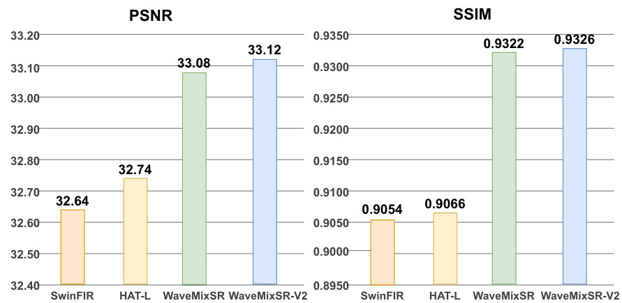
Figure 1: Comparison of PSNR and SSIM for $2\times$ SR on BSD100 dataset shows WaveMixSR-V2 surpasses the previous state-of-the-art WaveMixSR and other methods such as HAT and SwinFIR. $4\times$ SR results in Appendix.
图 1: 在BSD100数据集上进行的2倍超分辨率(Super-Resolution)PSNR与SSIM指标对比显示,WaveMixSR-V2超越了先前最先进的WaveMixSR以及HAT、SwinFIR等方法。4倍超分辨率结果见附录。
1 Introduction
1 引言
Single-image super-resolution (SISR) is a key task in image reconstruction, aiming to transform low-resolution (LR) images into high-resolution (HR) by predicting and restoring missing details. This process requires capturing both local information and global context. Recent advancements in super-resolution, particularly with attention-based transformers like SwinFIR [1] and hybrid attention transformer [2], have surpassed traditional CNN approaches due to their ability to capture long-range dependencies. However, transformers face challenges with quadratic complexity in self-attention, leading to high resource demands and requiring large datasets. To overcome this, token-mixer models such as WaveMixSR [3], which uses a two-dimensional discrete wavelet transform, have shown potential for improved efficiency and even superior performance. Building on the strengths of WaveMixSR, we propose enhancements to the model by rethinking its upsampling strategy inside the WaveMix blocks and changing the single stage design. Details of architecture, more results, including those on $4\times\mathrm{SR}$ , and ablation studies are provided in the Appendix.
单图像超分辨率 (SISR) 是图像重建中的关键任务,旨在通过预测和恢复缺失细节将低分辨率 (LR) 图像转换为高分辨率 (HR) 。该过程需要同时捕获局部信息和全局上下文。近年来,超分辨率领域的技术进步,尤其是基于注意力机制的 Transformer 模型(如 SwinFIR [1] 和混合注意力 Transformer [2]),因其能够捕捉长距离依赖关系,已超越传统的 CNN 方法。然而,Transformer 面临自注意力二次复杂度带来的挑战,导致资源需求高且依赖大规模数据集。为解决这一问题,诸如 WaveMixSR [3] 这类采用二维离散小波变换的 Token 混合器模型,已展现出提升效率甚至实现更优性能的潜力。基于 WaveMixSR 的优势,我们通过重新思考其 WaveMix 块内的上采样策略并调整单阶段设计,提出了模型改进方案。架构细节、更多结果(包括 $4\times\mathrm{SR}$ 的实验)以及消融研究详见附录。
2 Architectural Improvements
2 架构改进
2.1 Multi-stage Design
2.1 多阶段设计
We have made significant improvements to the WaveMixSR model, focusing on two key aspects. First, we addressed how the model handles SR tasks higher than $2\times$ . In the original WaveMixSR [3], all SR tasks were performed by directly resizing the LR image to HR using a single upsampling layer. This layer relied on non-parametric upsampling techniques, such as bilinear or bicubic interpolation, which limited the model’s ability to fine-tune and optimize the SR process across different scales. Our approach involved transitioning from this single-stage design to a more robust multi-stage design. In our new architecture, we introduced a series of resolution-doubling $2\times$ SR blocks, which progressively doubles the resolution step by step. This multi-stage approach allows for better SR performance at higher scales while reducing resource consumption.
我们对WaveMixSR模型进行了重大改进,重点聚焦于两个关键方面。首先,针对模型处理超过$2\times$的超分辨率(SR)任务的方式进行了优化。原始WaveMixSR [3]中,所有SR任务都是通过单个上采样层直接将低分辨率(LR)图像缩放到高分辨率(HR),该层依赖双线性或双三次插值等非参数化上采样技术,限制了模型在不同尺度下微调和优化SR过程的能力。我们的解决方案是将这种单阶段设计转变为更鲁棒的多阶段设计。在新架构中,我们引入了一系列分辨率翻倍的$2\times$ SR模块,逐步实现分辨率倍增。这种多阶段方法能在更高尺度下获得更好的SR性能,同时降低资源消耗。
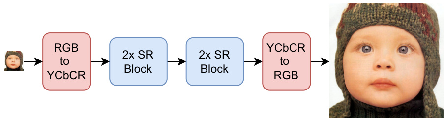
Figure 2: Architecture of WaveMixSR-V2 showing $4\times$ SR with two $2\times$ SR blocks in series. Details in Appendix.
图 2: WaveMixSR-V2架构示意图,展示通过两个串联的 $2\times$ 超分模块实现 $4\times$ 超分辨率。详见附录。
For instance, in an $4\times$ super-resolution task, instead of directly upsampling the LR image to HR using a single interpolation layer, the model now proceeds through a series of two $2\times$ SR blocks as shown in Fig. 2 By increment ally increasing the resolution (doubling in each stage), the model is better able to refine the details at each step, leading to superior super-resolution performance compared to the single upsampling operation used in the original WaveMixSR.
例如,在4倍超分辨率任务中,模型不再通过单一插值层直接将低分辨率(LR)图像上采样至高分辨率(HR),而是如图2所示依次通过两个2倍超分辨率块进行处理。通过分阶段逐步提升分辨率(每阶段翻倍),模型能更好地在每一步骤中优化细节,从而获得比原始WaveMixSR采用的单次上采样操作更优异的超分辨率性能。
2.2 Pixel Shuffle
2.2 像素洗牌 (Pixel Shuffle)
We introduce a key modification to the WaveMixSR model by replacing the transposed convolution operation in the WaveMix blocks with a Pixel Shuffle [4] operation followed by a convolution layer (WaveMixSR-V2 block) as shown in Fig. 5. While the original WaveMixSR used transposed convolutions, which involved numerous parameters and high computational cost, Pixel Shuffle upsamples the image more efficiently by rearranging pixels from feature maps. This significantly reduces the number of parameters, enhancing the model’s efficiency. The subsequent convolution layer after Pixel Shuffle allows the model to continue learning and refining features effectively. Moreover, Pixel Shuffle avoids the checkerboard artifacts commonly introduced by transposed convolutions, producing smoother and more natural-looking images while maintaining high-quality super-resolution outputs.
我们对WaveMixSR模型进行了一项关键改进:将WaveMix块中的转置卷积操作替换为Pixel Shuffle [4]操作后接卷积层(WaveMixSR-V2块),如图5所示。原始WaveMixSR使用的转置卷积涉及大量参数且计算成本高,而Pixel Shuffle通过重排特征图像素实现更高效的上采样。这显著减少了参数量,提升了模型效率。Pixel Shuffle后接的卷积层使模型能持续有效地学习和优化特征。此外,Pixel Shuffle避免了转置卷积常见的棋盘伪影,在保持高质量超分辨率输出的同时,能生成更平滑自然的图像。
Incorporating these improvements in the architecture has enabled WaveMixSR-V2 to achieve new state-of-the-art (SOTA) performance on the BSD100 dataset [5]. Notably, it accomplishes this with less than half the number of parameters, lesser computations and lower latency compared to WaveMixSR (previous SOTA).
将这些改进融入架构后,WaveMixSR-V2在BSD100数据集[5]上实现了新的最先进(SOTA)性能。值得注意的是,与WaveMixSR(前SOTA)相比,它用不到一半的参数数量、更少的计算量和更低的延迟实现了这一目标。
References
参考文献
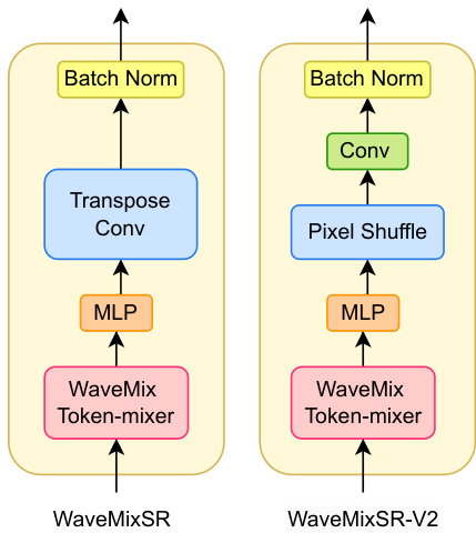
Figure 3: Simplified block diagram of WaveMix block in WaveMixSR (on the left) and WaveMixSR-V2 block (on the right). Details in Appendix.
Table 1: Model complexity comparison of WaveMixSR-V2 with other state-of-the-art methods such as WaveMixSR, SwinIR and HAT on $4\times\mathrm{SR}$ of $64\times64$ input patch.
图 3: WaveMixSR 中的 WaveMix 模块简化框图(左)和 WaveMixSR-V2 模块(右)。详情见附录。
| 模型 | 参数量 | 乘加运算量 |
|---|---|---|
| SwinIR [6] | 11.8M | 49.6G |
| HAT [2] | 20.8M | 103.7G |
| WaveMixSR[3] | 1.7M | 25.8G |
| WaveMixSR-V2 | 0.7M | 25.6G |
表 1: WaveMixSR-V2 与其他先进方法(如 WaveMixSR、SwinIR 和 HAT)在 $64\times64$ 输入块 $4\times\mathrm{SR}$ 任务上的模型复杂度对比。
A Architecture
架构
A.1 WaveMixSR-V2 Block
A.1 WaveMixSR-V2 模块
The core part of our super-resolution (SR) architecture are the WaveMixSR-V2 blocks shown in Fig. 4(c). We created these by modifying the WaveMix [7] blocks used in WaveMixSR model [3]. We replace the transposed convolution used in WaveMix block with a Pixel Shuffle [4] operation followed by a convolutional layer.
我们超分辨率 (SR) 架构的核心部分是图 4(c) 所示的 WaveMixSR-V2 模块。这些模块是通过修改 WaveMixSR 模型 [3] 中使用的 WaveMix [7] 模块而创建的。我们将 WaveMix 模块中使用的转置卷积替换为 Pixel Shuffle [4] 操作,后接一个卷积层。
Denoting input and output tensors of the WaveMixSR-V2 block by ${\bf{X}}{i n}$ and $\mathbf{X}{O u t}$ , respectively; the four wavelet filters along with their down sampling operations at each level by $w_{a a},w_{a d},w_{d a},w_{d d}$ ( $\mathit{\check{a}}$ for approximation, $d$ for detail); convolution, multi-layer perceptron (MLP), Pixel Shuffle, and batch normalization operations by $c,m,p$ , and $b$ , respectively; and their respective trainable parameter sets by $\xi,\theta,\phi$ , and $\gamma$ , respectively; concatenation along the channel dimension by $\bigoplus$ , and point-wise addition by $^+$ , the operations inside a WaveMixSR-V2 block can be expressed using the following equations:
将 WaveMixSR-V2 块的输入和输出张量分别表示为 ${\bf{X}}{i n}$ 和 $\mathbf{X}{O u t}$;四个小波滤波器及其每层的下采样操作为 $w_{a a},w_{a d},w_{d a},w_{d d}$($\mathit{\check{a}}$ 表示近似,$d$ 表示细节);卷积、多层感知机 (MLP)、Pixel Shuffle 和批量归一化操作分别表示为 $c,m,p$ 和 $b$;它们各自的可训练参数集分别为 $\xi,\theta,\phi$ 和 $\gamma$;沿通道维度的拼接操作为 $\bigoplus$,逐点相加操作为 $^+$,则 WaveMixSR-V2 块内的操作可用以下公式表示:
$$
\mathbf{x}{0}=c(\mathbf{x}{i n},\boldsymbol{\xi});~\mathbf{x}{i n}\in\mathbb{R}^{H\times W\times C},\mathbf{x}_{0}\in\mathbb{R}^{H\times W\times C/4}
$$
$$
\mathbf{x}{0}=c(\mathbf{x}{i n},\boldsymbol{\xi});~\mathbf{x}{i n}\in\mathbb{R}^{H\times W\times C},\mathbf{x}_{0}\in\mathbb{R}^{H\times W\times C/4}
$$
$$
\mathbf{x}=[w_{a a}(\mathbf{x}{0})\oplus w_{a d}(\mathbf{x}{0})\oplus w_{d a}(\mathbf{x}{0})\oplus w_{d d}(\mathbf{x}_{0})];~\mathbf{x}\in\mathbb{R}^{H/2\times W/2\times4C/4}
$$
$$
\mathbf{x}=[w_{a a}(\mathbf{x}{0})\oplus w_{a d}(\mathbf{x}{0})\oplus w_{d a}(\mathbf{x}{0})\oplus w_{d d}(\mathbf{x}_{0})];~\mathbf{x}\in\mathbb{R}^{H/2\times W/2\times4C/4}
$$
$$
\tilde{\mathbf{x}}=b(c(p(m(\mathbf{x},\theta),\phi),\xi),\gamma);~\tilde{\mathbf{x}}\in\mathbb{R}^{H\times W\times C}
$$
$$
\tilde{\mathbf{x}}=b(c(p(m(\mathbf{x},\theta),\phi),\xi),\gamma);~\tilde{\mathbf{x}}\in\mathbb{R}^{H\times W\times C}
$$
$$
\mathbf{x}{o u t}=\tilde{\mathbf{x}}{1}+\mathbf{x}{i n};\qquad\mathbf{x}_{o u t}\in\mathbb{R}^{H\times W\times C}
$$
$$
\mathbf{x}{o u t}=\tilde{\mathbf{x}}{1}+\mathbf{x}{i n};\qquad\mathbf{x}_{o u t}\in\mathbb{R}^{H\times W\times C}
$$
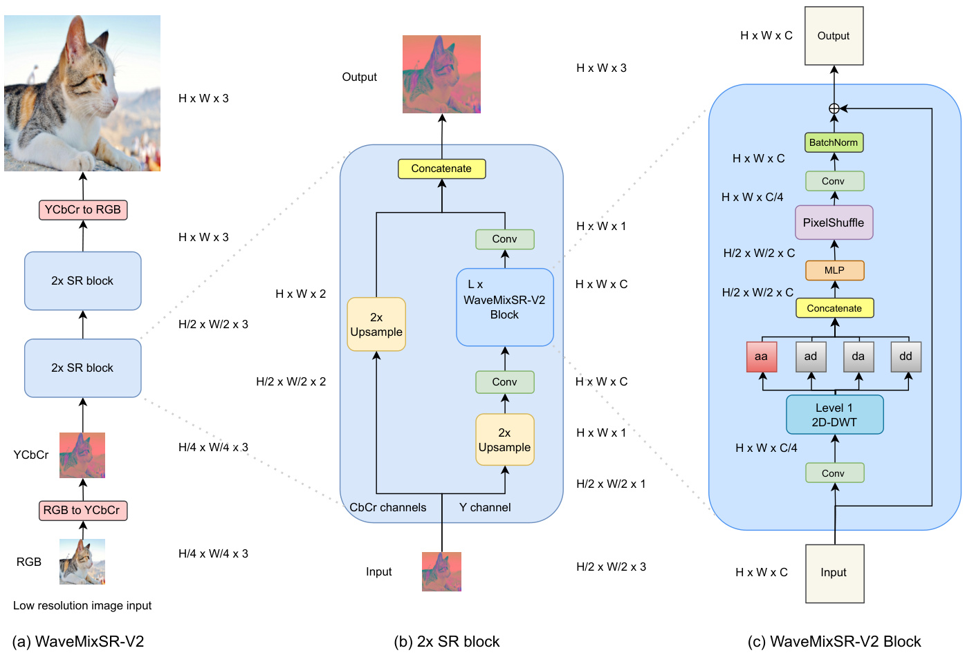
Figure 4: Architecture of WaveMixSR-V2. (a) The application of WaveMixSR-V2 for $4\times$ SR is shown featuring two $2\times$ SR blocks stacked in series. For higher SR tasks, more $2\times$ SR blocks will be added. (b) The details of the $2\times\mathrm{SR}$ block and (c) shows the WaveMixSR-V2 block that replaces the transposed convolution with a Pixel Shuffle operation followed by a convolution.
图 4: WaveMixSR-V2架构。(a) 展示了WaveMixSR-V2在$4\times$超分辨率(SR)任务中的应用,采用两个串联的$2\times$ SR模块堆叠而成。对于更高倍率的SR任务,将添加更多$2\times$ SR模块。(b) $2\times\mathrm{SR}$模块的详细结构,(c) 展示了用Pixel Shuffle操作替代转置卷积、后接常规卷积的WaveMixSR-V2模块。
The WaveMixSR-V2 block extracts learnable and space-invariant features using a convolutional layer, followed by spatial token-mixing and down sampling for scale-invariant feature extraction using 2 dimenional-discrete wavelet transform (2D-DWT) [13], followed by channel-mixing using a learnable MLP ( $1\times1$ conv) layer, followed by restoring spatial resolution of the feature map using Pixel Shuffle operation. The use of trainable convolutions before the wavelet transform allows the extraction of only those feature maps that are suitable for the chosen wavelet basis functions. The convolutional layer $c$ decreases the embedding dimension $C$ by a factor of four so that the concatenated output $\mathbf{X}$ after 2D-DWT has the same number of channels as the input ${\bf{X}}_{i n}$ (Eq.1 and Eq.2). That is since 2D-DWT is a lossless transform, it expands the number of channels by the same factor (using concatenation) by which it reduces the spatial resolution by computing an approximation sub-band (low-resolution approximation) and three detail sub-bands (spatial derivatives) [14] for each input channel (Eq.2). The use of this image-appropriate and lossless down sampling using 2D-DWT allows WaveMixSR-V2 to use fewer layers and parameters.
WaveMixSR-V2模块通过卷积层提取可学习且空间不变的特征,随后进行空间token混合,并利用二维离散小波变换(2D-DWT) [13]进行尺度不变特征的下采样,接着通过可学习的MLP( $1\times1$ 卷积)层进行通道混合,最后使用Pixel Shuffle操作恢复特征图的空间分辨率。在小波变换前使用可训练卷积层,能够仅提取适合所选小波基函数的特征图。卷积层 $c$ 将嵌入维度 $C$ 缩减为四分之一,使得2D-DWT后的拼接输出 $\mathbf{X}$ 与输入 ${\bf{X}}_{i n}$ 保持相同通道数(式1与式2)。由于2D-DWT是无损变换,它通过计算每个输入通道的近似子带(低分辨率近似)和三个细节子带(空间导数) [14] (式2),在降低空间分辨率的同时以相同倍数(通过拼接)扩展通道数。这种基于图像特性且无损的2D-DWT下采样方式,使得WaveMixSR-V2能够使用更少的层数和参数。
The output $\hat{\bf x}$ is then passed to an MLP layer $m$ , which has two $1\times1$ convolutional layers with an inverse bottleneck design (multiplication factor $>1$ ) separated by a GELU non-linearity. After this, the feature map resolution is doubled using Pixel Shuffle operation $p$ . Since Pixel Shuffle reduces the channel dimension by 4, we use another convolution layer $c$ to increase the channel dimension back to $C$ . This is followed by batch normalization $b$ (Eq.3). A residual connection is used to ease the flow of the gradient [15] (Eq.4). The WaveMixSR-V2 block ensures that input and output resolution are the same.
输出 $\hat{\bf x}$ 随后被传递到一个 MLP 层 $m$,该层采用逆瓶颈设计(乘数因子 $>1$),包含两个 $1\times1$ 卷积层,中间通过 GELU 非线性激活函数分隔。此后,使用 Pixel Shuffle 操作 $p$ 将特征图分辨率提升一倍。由于 Pixel Shuffle 会将通道维度减少 4 倍,我们通过另一个卷积层 $c$ 将通道维度恢复至 $C$,随后进行批量归一化 $b$(式3)。采用残差连接以优化梯度流动 [15](式4)。WaveMixSR-V2 模块确保输入与输出分辨率保持一致。
Among the different types of mother wavelets available, we used the Haar wavelet (a special case of the Daubechies wavelet [14], also known as Db1), which is frequently used due to its simplicity and faster computation. Haar wavelet is both orthogonal and symmetric in nature and has been extensively used to extract basic structural information from images [16]. For even-sized images, it reduces the dimensions exactly by a factor of 2, which simplifies the designing of the subsequent layers.
在可选的小波基函数中,我们采用了Haar小波(Daubechies小波[14]的特例,亦称Db1)。因其计算简单高效而广受青睐,Haar小波兼具正交性与对称性,已被广泛应用于图像基础结构信息提取[16]。对于偶数尺寸图像,它能将维度精确缩减为原尺寸的1/2,从而简化后续网络层的设计。
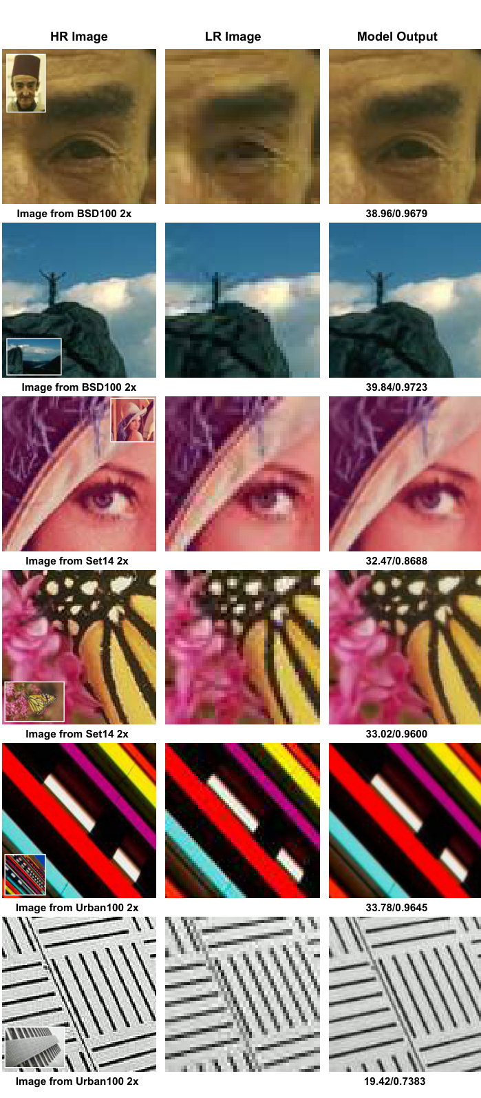
Figure 5: Visual results of $2\times$ SR on BSD100 dataset. Each column from the left shows a patch from the HR image (shown as a small image near the corner), the same patch extracted from the LR image, and a patch taken from the model output respectively. The filename of the image is given below the HR image and the PSNR/SSIM of the model output is reported at below the model output. The values displayed are computed for the whole image and not just the patch.
图 5: BSD100 数据集上 $2\times$ 超分辨率 (SR) 的视觉结果。从左至右每列分别显示:HR (高分辨率) 图像中的局部区块 (角落以小图展示)、从 LR (低分辨率) 图像提取的相同区块、模型输出对应的区块。HR 图像下方标注文件名,模型输出下方显示其 PSNR/SSIM 指标。所示数值为整幅图像 (而非局部区块) 的计算结果。
Table 2: Quantitative comparison with previous state-of-the-art methods on the BSD100 dataset shows that WaveMixSRV2 performs better using less training data ( $^*$ indicates models that were pre-trained on ImageNet).
表 2: 在BSD100数据集上与先前最先进方法的定量比较表明,WaveMixSRV2使用更少的训练数据表现更好($^*$表示在ImageNet上预训练的模型)。
| 模型 | 训练数据集 | 2× SR PSNR | 2× SR SSIM | 4× SR PSNR | 4× SR SSIM |
|---|---|---|---|---|---|
| EDSR [8] | DIV2K | 32.32 | 0.9013 | 27.71 | 0.7420 |
| RCAN [9] | DIV2K | 32.41 | 0.9027 | 27.77 | 0.7436 |
| SAN [10] | DIV2K | 32.42 | 0.9028 | 27.78 | 0.7436 |
| IGNN [10] | DIV2K | 32.41 | 0.9025 | 27.77 | 0.7434 |
| HAN [11] | DIV2K | 32.41 | 0.9027 | 27.80 | 0.7442 |
| NLSN [10] | DIV2K | 32.43 | 0.9027 | 27.78 | 0.7444 |
| RCN-it [10] | DF2K | 32.48 | 0.9034 | 27.87 | 0.7459 |
| SwinIR [6] | DF2K | 32.53 | 0.9041 | 27.92 | 0.7489 |
| EDT [12] | DF2K | 32.52 | 0.9041 | 27.91 | 0.7483 |
| HAT [10] | DF2K | 32.62 | 0.9053 | 28.00 | 0.7517 |
| SwinFIR* [1] | DF2K | 32.64 | 0.9054 | 28.03 | 0.7520 |
| HAT-L* [10] | DF2K | 32.74 | 0.9066 | 28.09 | 0.7551 |
| WaveMixSR [3] | DIV2K | 33.08 | 0.9322 | 27.65 | 0.7605 |
| WaveMixSR-V2 | DIV2K | 33.12 | 0.9326 | 27.87 | 0.7640 |
Table 3: Comparison of latency and throughput of WaveMixSR-V2 and WaveMixSR shows that WaveMixSR-V2 is significantly faster than WaveMixSR
| 模型 | 训练延迟 ← (毫秒) | 训练吞吐量 (帧/秒) | 推理延迟 ↓ (毫秒) | 推理吞吐量 ↑ (帧/秒) |
|---|---|---|---|---|
| WaveMixSR | 22.8 | 43.8 | 18.6 | 53.7 |
| WaveMixSR-V2 | 19.6 | 50.8 | 12.1 | 82.6 |
表 3: WaveMixSR-V2与WaveMixSR的延迟和吞吐量对比表明,WaveMixSR-V2显著快于WaveMixSR
A.2 $2\times$ SR Block
A.2 $2\times$ SR 块
As shown in Fig. 4(b), the $2\times\mathrm{SR}$ block has two paths – one for handling the Y channel and another for the CbCr channels of the input image. The Y channel is used for the path with learning using WaveMixSR-V2 blocks because the Y channel contains most of the image details and is less affected by color changes. It first upsamples the image to HR size using a parameter-free upsampling block using bilinear or bicubic interpolation. The output of upsampling block, is sent to a convolutional layer to increase the number of feature maps before sending it to the WaveMixSR-V2 blocks. We connected $L$ WaveMixSR-V2 blocks in series to create high-resolution feature maps. The output from the final WaveMixSR-V2 blocks is then passed through a convolutional layer which reduces the channel dimension and returns a single channel output.
如图4(b)所示,$2\times\mathrm{SR}$模块包含两条路径——一条处理输入图像的Y通道,另一条处理CbCr通道。Y通道路径采用WaveMixSR-V2块进行学习,因为Y通道包含图像大部分细节且受色彩变化影响较小。该路径首先通过双线性/双三次插值的无参数上采样模块将图像上采样至高分辨率(HR)尺寸,随后通过卷积层增加特征图数量,再输入至WaveMixSR-V2块。我们将$L$个WaveMixSR-V2块串联以生成高分辨率特征图,最终通过卷积层降维输出单通道结果。
Table 4: Quantitative results of WaveMixSR-V2 on other benchmark SR datasets
| 尺度 | 2x | 4x |
|---|---|---|
| PSNR | SSIM | |
| Set5 | 35.85 | 0.9522 |
| Set14 | 31.20 | 0.9000 |
| Urban100 | 29.20 | 0.9076 |
表 4: WaveMixSR-V2 在其他基准超分辨率数据集上的定量结果
Table 5: Quantitative comparison of WaveMixSR-V2 on benchmark datasets when using different combination of losses for various input resolutions.
表 5: WaveMixSR-V2 在不同输入分辨率下使用不同损失组合时在基准数据集上的定量比较。
| 输入分辨率 | 像素损失 入o | 内容损失 入1 | 对抗损失 入2 | 是否添加噪声 | BSD100 PSNR | BSD100 SSIM | Set5 PSNR | Set5 SSIM | Set14 PSNR | Set14 SSIM | Urban100 PSNR | Urban100 SSIM |
|---|---|---|---|---|---|---|---|---|---|---|---|---|
| 128 × 128 | 1 | 0.01 | 0.001 | 是 | 28.39 | 0.8816 | 30.16 | 0.8996 | 27.76 | 0.8667 | 25.14 | 0.8520 |
| 64 × 64 | 1 | 0.01 | 0.001 | 是 | 28.62 | 0.8661 | 29.96 | 0.8728 | 27.67 | 0.8421 | 25.24 | 0.8368 |
| 128 × 128 | 1 | 0 | 0.01 | 是 | 30.02 | 0.9065 | 31.01 | 0.9146 | 28.46 | 0.8756 | 25.78 | 0.8584 |
| 64 × 64 | 1 | 0 | 0.01 | 是 | 30.23 | 0.9023 | 30.84 | 0.9121 | 28.41 | 0.8154 | 25.93 | 0.8434 |
| 128 × 128 | 1 | 0.01 | 0.001 | 否 | 29.36 | 0.9008 | 30.46 | 0.9064 | 27.58 | 0.8660 | 25.02 | 0.8476 |
| 64 × 64 | 1 | 0.01 | 0.001 | 否 | 28.09 | 0.8815 | 29.48 | 0.8918 | 27.34 | 0.8664 | 24.83 | 0.8474 |
| 128 × 128 | 1 | 0 | 0 | 否 | 31.24 | 0.9267 | 33.12 | 0.9398 | 29.44 | 0.8957 | 26.49 | 0.8780 |
| 64 × 64 | 1 | 0 | 0 | 否 | 31.19 | 0.9263 | 32.91 | 0.9378 | 29.38 | 0.8948 | 26.46 | 0.8772 |
Table 6: Results of ablation studies showing performance when we vary the channel dimension and layers of WaveMixSR-V2 blocks.
| 通道维度 | 层深度 | BSD100 PSNR | BSD100 SSIM | Set5 PSNR | Set5 SSIM | Set14 PSNR | Set14 SSIM | Urban100 PSNR | Urban100 SSIM |
|---|---|---|---|---|---|---|---|---|---|
| 144 | 4 | 31.16 | 0.9267 | 33.00 | 0.9401 | 29.38 | 0.8964 | 26.45 | 0.8785 |
| 160 | 4 | 31.16 | 0.9267 | 32.97 | 0.9400 | 29.38 | 0.8960 | 26.46 | 0.8786 |
| 144 | 6 | 31.19 | 0.9263 | 32.91 | 0.9378 | 29.38 | 0.8948 | 26.46 | 0.8772 |
表 6: 消融研究结果展示了WaveMixSR-V2模块通道维度和层数变化时的性能表现。
The second parallel path takes the two CbCr channels and passes it through an upsampling layer where the resolution is doubled. This HR CbCr channel is concatenated with the Y-channel output from the first path, thereby creating the 3-channel YCbCr HR output, which is converted to RGB to obtain the doubled resolution output image.
第二条并行路径处理两个CbCr通道,通过一个上采样层使分辨率翻倍。这个高分辨率CbCr通道与第一条路径输出的Y通道拼接,从而生成3通道的YCbCr高分辨率输出,再转换为RGB格式得到分辨率翻倍的输出图像。
A.3 WaveMixSR-V2
A.3 WaveMixSR-V2
The LR input image in RGB space is first converted to YCbCr space before sending to the model as shown Fig. 4(a). It is then passed through a series of $2\times\mathrm{SR}$ blocks. For $2\times\mathrm{SR}$ , we use just one $2\times$ SR block. For higher SR tasks, we can modify the network by adding as many $2\times$ SR blocks as required to achieve as much SR as needed, as adding one $2\times$ SR block doubles the resolution. Finally, the output from $2\times$ SR blocks are converted back to RGB space to get final output.
RGB空间中的LR输入图像在送入模型前会先转换为YCbCr空间,如图4(a)所示。随后图像会通过一系列$2\times\mathrm{SR}$模块进行处理。对于$2\times\mathrm{SR}$任务,我们仅使用一个$2\times$SR模块。针对更高倍率的超分任务,可通过叠加所需数量的$2\times$SR模块来灵活调整网络结构(每增加一个$2\times$SR模块分辨率即翻倍)。最终,$2\times$SR模块的输出会被转换回RGB空间形成最终结果。
B Implementation Details
B 实现细节
We used DIV2K dataset [17] for training WaveMixSR-V2. We did not employ any pre-training on larger datasets such as DF2K [17] or ImageNet [18] to compare the performance in training data-constrained settings. The performance of WaveMixSR-V2 was tested on four benchmark datasets – BSD100 [19], Urban100 [20], Set5 [21], and Set14 [22], .
我们使用DIV2K数据集[17]来训练WaveMixSR-V2。为了比较在训练数据受限情况下的性能,我们没有在DF2K[17]或ImageNet[18]等更大数据集上进行任何预训练。WaveMixSR-V2的性能在四个基准数据集上进行了测试——BSD100[19]、Urban100[20]、Set5[21]和Set14[22]。
All experiments were done with a single 48 GB Nvidia A6000 GPU. We used AdamW optimizer $(\alpha=0.001,\beta_{1}=$ $0.9,\beta_{2}=0.999$ , $\epsilon=10^{-8}.$ ) with a weight decay of 0.01 during initial epochs and then used SGD with a learning rate of 0.001 and momentum $=0.9$ during the final 50 epochs [23, 24]. A dropout of 0.3 is used in our experiments. A batch size of 1 was used when the full-resolution images were passed to the model and a batch size of 432 was used when images were passed as $64\times64$ resolution patches.
所有实验均使用单块48GB显存的Nvidia A6000 GPU完成。我们采用AdamW优化器 $(\alpha=0.001,\beta_{1}=$ $0.9,\beta_{2}=0.999$ , $\epsilon=10^{-8}.$ ),初始阶段权重衰减设为0.01,最后50个epoch改用学习率0.001、动量 $=0.9$ 的SGD优化器 [23, 24]。实验中使用0.3的dropout率。当输入全分辨率图像时批处理大小为1,输入 $64\times64$ 分辨率图像块时批处理大小为432。
The LR images were generated from the HR images by using bicubic down-sampling in Pytorch. We used the fullresolution HR image as the target and generated the input LR image using down-sampling for each of the SR tasks. No data augmentations were used while training the WaveMixSR-V2 models. Huber loss was used to optimize the parameters. We used automatic mixed precision in PyTorch during training. For the quantitative results, PSNR and SSIM (calculated on the $\mathrm{Y}$ channel) are reported.
LR图像是通过在PyTorch中使用双三次下采样从HR图像生成的。我们将全分辨率HR图像作为目标,并为每个超分辨率(SR)任务通过下采样生成输入LR图像。训练WaveMixSR-V2模型时未使用数据增强。采用Huber损失函数优化参数。训练期间在PyTorch中启用了自动混合精度。定量结果报告了PSNR和SSIM(基于$\mathrm{Y}$通道计算)。
The embedding dimension of 144 was used in WaveMixSR-V2 blocks. The convolutions layers before and after the WaveMixSR-V2 blocks which were used to vary channel dimensions employed $3\times3$ kernels with stride and padding set to 1 to maintain the feature resolution.
WaveMixSR-V2 模块采用了 144 的嵌入维度 (embedding dimension)。模块前后用于调整通道维度的卷积层均使用 $3\times3$ 核 (kernel),并将步长 (stride) 和填充 (padding) 设为 1 以保持特征分辨率。
C Results
C 结果
From Table 2, it is evident that WaveMixSR-V2 has achieved state-of-the-art (SOTA) performance in $2\times$ and $4\times$ SR tasks on the BSD100 dataset. WaveMixSR-V2 attains this superior performance while utilizing significantly smaller DIV2K training data compared to other models, which typically rely on the much larger DF2K and ImageNet datasets. Even in the PSNR metric for $4\times$ SR, WaveMixSR-V2 is SOTA among all models trained solely on the smaller DIV2K dataset. In contrast, all models that outperform WaveMixSR-V2 in $4\times$ SR PSNR have been trained on the much larger DF2K data and even have leveraged ImageNet pre-training, further underscoring WaveMixSR-V2’s efficiency in achieving SOTA results with fewer training data.
从表2可以明显看出,WaveMixSR-V2在BSD100数据集的$2\times$和$4\times$超分辨率(SR)任务中实现了最先进(SOTA)性能。与其他通常依赖更大规模DF2K和ImageNet数据集的模型相比,WaveMixSR-V2仅使用显著更小的DIV2K训练数据就取得了这一卓越性能。即使在$4\times$超分辨率的PSNR指标上,WaveMixSR-V2也是仅使用较小DIV2K数据集训练的所有模型中的SOTA。相比之下,所有在$4\times$超分辨率PSNR上优于WaveMixSR-V2的模型都使用了更大的DF2K数据进行训练,甚至利用了ImageNet预训练,这进一步凸显了WaveMixSR-V2以更少训练数据实现SOTA结果的高效性。
Table 3 provides a comparison of latency and throughput for WaveMixSR-V2 compared to its predecessor, WaveMixSR. WaveMixSR had previously set the benchmark for efficiency, known for its fast output, low GPU consumption, and parametric efficiency in SR tasks. However, WaveMixSR-V2 surpasses its predecessor with faster training and inference speeds. As shown in the Table 3, WaveMixSR-V2 exhibits a much lower latency and significantly higher throughput, both in training $(\sim15%$ improvement) and inference ( $54%$ improvement), cementing its status as one of the most efficient models for super-resolution.
表 3: 对比了 WaveMixSR-V2 与其前身 WaveMixSR 在延迟和吞吐量方面的表现。WaveMixSR 曾以快速输出、低 GPU 消耗和超分辨率 (SR) 任务中的参数效率著称,为效率设定了基准。然而,WaveMixSR-V2 在训练和推理速度上均超越了前代。如表 3 所示,WaveMixSR-V2 在训练 (提升约 15%) 和推理 (提升 54%) 中均展现出更低的延迟和显著更高的吞吐量,巩固了其作为超分辨率领域最高效模型之一的地位。
In Table 3, we present the quantitative metrics for the results of $2\times$ and $4\times$ SR across various benchmark datasets, such as Set5, Set14, and Urban100. These datasets are widely used for evaluating super-resolution models. The results demonstrate that WaveMixSR-V2 performs competitively, delivering excellent outcomes in both $2\times$ and $4\times\mathrm{SR}$ tasks across all datasets.
在表3中,我们展示了在不同基准数据集(如Set5、Set14和Urban100)上进行2倍和4倍超分辨率(SR)的定量指标。这些数据集被广泛用于评估超分辨率模型。结果表明,WaveMixSR-V2在所有数据集上的2倍和4倍SR任务中都具有竞争力,并取得了优异的结果。
D Ablation Studies
D 消融研究
D.1 WaveMixSR-V2 GAN
D.1 WaveMixSR-V2 GAN
We conducted experiments to check the performance of the WaveMixSR-V2 architecture when trained using a Generative Adversarial Network (GAN) framework, incorporating a relativistic disc rim in at or [?] with residual connections. We also experimented the impact of introducing Gaussian noise as an extra input channel alongside the RGB channels. The hypothesis was that this noise might enhance the HR quality by encouraging the model to incorporate higher frequency components. The experiments used images from the DIV2K dataset resized to different dimensions for training and were evaluated on benchmarks datasets.
我们通过实验验证了WaveMixSR-V2架构在生成对抗网络 (Generative Adversarial Network, GAN) 框架下训练的性能,该框架结合了相对论判别器与残差连接。我们还测试了在RGB通道之外引入高斯噪声作为额外输入通道的效果,假设这种噪声可能通过促使模型融合更高频分量来提升高分辨率 (HR) 输出质量。实验采用DIV2K数据集的多尺度缩放图像进行训练,并在基准数据集上评估性能。
D.1.1 Loss
D.1.1 损失函数
In terms of loss functions, we used a combination of pixel loss $(L_{p i x e l})$ , content loss $(L_{c o n t e n t})$ [25], and adversarial loss. The pixel loss was based on the Peak Signal-to-Noise Ratio (PSNR) to directly optimize the model for higher PSNR values. For content loss, a pre-trained VGG19 model was used as the feature extractor. Specifically, features were extracted from the 5th convolutional layer before the 4th max-pooling layer of the VGG-19 model. The adversarial loss was computed using a binary cross-entropy loss with logits on the output of the disc rim in at or, comparing the predictions for real and generated images. The adversarial loss was to guide the generator to produce more realistic images, improving the fidelity of higher-frequency details.
在损失函数方面,我们结合使用了像素损失 $(L_{p i x e l})$、内容损失 $(L_{c o n t e n t})$ [25] 和对抗损失。像素损失基于峰值信噪比 (PSNR) ,直接优化模型以获得更高的 PSNR 值。内容损失采用预训练的 VGG19 模型作为特征提取器,具体从 VGG-19 模型第 4 个最大池化层前的第 5 个卷积层提取特征。对抗损失通过判别器输出的二元交叉熵对数损失计算,对比真实图像与生成图像的预测结果,其作用是引导生成器产生更逼真的图像,从而提升高频细节的保真度。
The overall loss function combined pixel loss, content loss, and adversarial loss as follows:
整体损失函数结合了像素损失 (pixel loss) 、内容损失 (content loss) 和对抗损失 (adversarial loss) ,如下所示:
$$
L o s s=\lambda_{0}L_{p i x e l}+\lambda_{1}L_{c o n t e n t}+\lambda_{2}L_{a d v e r s a r i a l}
$$
$$
L o s s=\lambda_{0}L_{p i x e l}+\lambda_{1}L_{c o n t e n t}+\lambda_{2}L_{a d v e r s a r i a l}
$$
where $\lambda_{0},\lambda_{1}$ and $\lambda_{2}$ are hyper parameters that control the relative importance of content loss and adversarial loss, respectively.
其中 $\lambda_{0},\lambda_{1}$ 和 $\lambda_{2}$ 是控制内容损失和对抗损失相对重要性的超参数。
The variation in content loss ratios significantly influenced the model’s performance. When the content loss ratio was reduced to zero, the model was able to focus more on low-frequency components, leading to an improvement in PSNR and SSIM values across the datasets. For instance, with an input resolution of $128\times128$ , setting the content loss ratio to zero resulted in a noticeable increase in performance, as the model could better optimize for low-frequency details. In contrast, when a content loss ratio was included, it forced the training slightly toward including more high-frequency components. However, the WaveMixSR-V2 architecture struggled to learn these components effectively, leading to sub-optimal performance compared to the scenario where content loss was not used.
内容损失比例的变化显著影响了模型的性能。当内容损失比例降至零时,模型能够更专注于低频成分,从而在所有数据集中提升PSNR和SSIM值。例如,在输入分辨率为$128\times128$时,将内容损失比例设为零会带来明显的性能提升,因为模型能更好地优化低频细节。相反,当包含内容损失比例时,训练会略微偏向包含更多高频成分。然而,WaveMixSR-V2架构难以有效学习这些成分,导致性能逊于未使用内容损失的情况。
D.1.2 Gaussian Noise
D.1.2 高斯噪声 (Gaussian Noise)
Regarding the addition of Gaussian noise, the results were mixed. An improvement was observed when using an input resolution of $64\times64$ , where the PSNR and SSIM values increased, suggesting that the noise channel helped the model capture finer details and potentially enhance the perceptual quality of the images. However, when we increased the input resolution to $128\times128$ , the inclusion of noise led to a slight decrease in performance. This indicates that the effectiveness of adding noise may depend on the input resolution and the model’s ability to utilize this additional information effectively.
关于添加高斯噪声的结果好坏参半。在使用 $64\times64$ 输入分辨率时观察到改进,PSNR 和 SSIM 值有所提升,这表明噪声通道帮助模型捕捉更精细的细节,并可能增强图像的感知质量。然而,当我们将输入分辨率提高到 $128\times128$ 时,加入噪声会导致性能略有下降。这表明添加噪声的效果可能取决于输入分辨率以及模型有效利用这一额外信息的能力。
Interestingly, regular training of WaveMixSR-V2 using just PSNR as the pixel loss provided considerably better performance than GAN training. This could be due to the fundamental difference in how WaveMixSR-V2 and GANs handle frequency components in images. While GAN training typically forces the network to include more high-frequency details to enhance visual fidelity, WaveMixSR-V2 focuses more on low-frequency components. This divergence in focus likely led to a mismatch during training, making it challenging for the model to converge effectively under the GAN training. Consequently, the benefits of using GAN training with WaveMixSR-V2 were limited, as the architecture’s emphasis on low-frequency components did not align well with the GAN’s objectives.
有趣的是,仅使用PSNR作为像素损失对WaveMixSR-V2进行常规训练,其性能明显优于GAN训练。这可能源于WaveMixSR-V2与GAN在图像频率成分处理上的本质差异:GAN训练通常强制网络包含更多高频细节以提升视觉保真度,而WaveMixSR-V2更侧重于低频成分。这种关注点的差异可能导致训练过程中的不匹配,使得模型在GAN训练下难以有效收敛。因此,将GAN训练应用于WaveMixSR-V2的收益有限,因为该架构对低频成分的侧重与GAN的目标并不契合。