Pix3D: Dataset and Methods for Single-Image 3D Shape Modeling
Pix3D: 单图像3D形状建模数据集与方法
Xingyuan Sun∗1,2 Jiajun Wu∗1 Xiuming Zhang1 Zhoutong Zhang1 Chengkai Zhang1 Tianfan Xue3 Joshua B. Tenenbaum1 William T. Freeman1,3
Xingyuan Sun∗1,2 Jiajun Wu∗1 Xiuming Zhang1 Zhoutong Zhang1 Chengkai Zhang1 Tianfan Xue3 Joshua B. Tenenbaum1 William T. Freeman1,3
1 Massachusetts Institute of Technology 2Shanghai Jiao Tong University 3Google Research
1 麻省理工学院 2 上海交通大学 3 Google Research
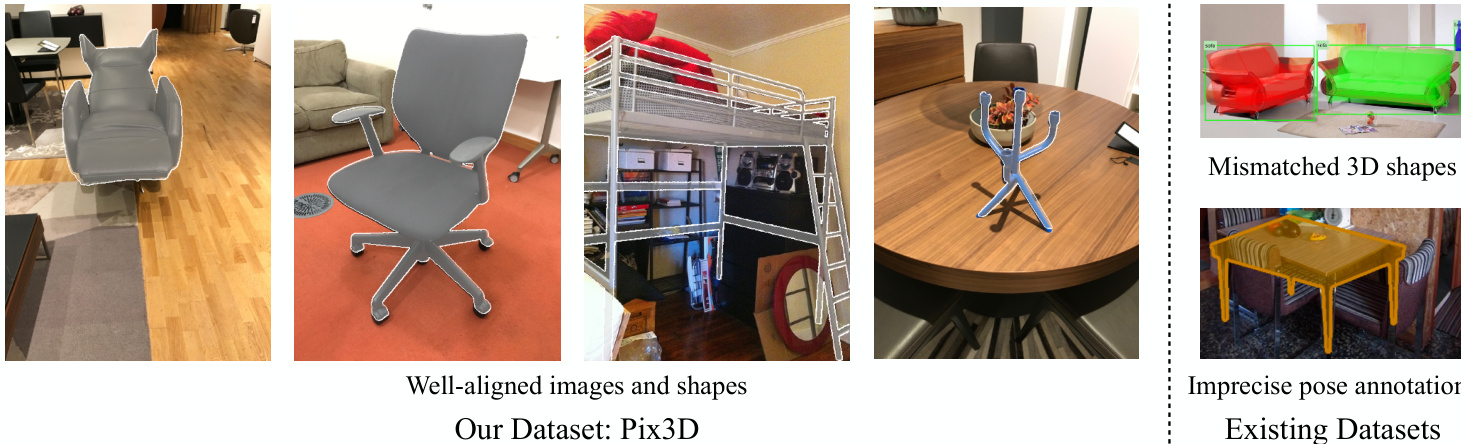
Figure 1: We present Pix3D, a new large-scale dataset of diverse image-shape pairs. Each 3D shape in Pix3D is associated with a rich and diverse set of images, each with an accurate 3D pose annotation to ensure precise 2D-3D alignment. In comparison, existing datasets have limitations: 3D models may not match the objects in images; pose annotations may be imprecise; or the dataset may be relatively small.
图 1: 我们提出了Pix3D——一个包含多样化图像-形状对的大规模新数据集。Pix3D中的每个3D形状都关联着一组丰富多样的图像,每张图像都带有精确的3D位姿标注以确保2D-3D对齐的准确性。相比之下,现有数据集存在以下局限:3D模型可能与图像中的物体不匹配;位姿标注可能不精确;或者数据集规模相对较小。
Abstract
摘要
We study 3D shape modeling from a single image and make contributions to it in three aspects. First, we present Pix3D, a large-scale benchmark of diverse image-shape pairs with pixel-level 2D-3D alignment. Pix3D has wide applications in shape-related tasks including reconstruction, retrieval, viewpoint estimation, etc. Building such a large-scale dataset, however, is highly challenging; existing datasets either contain only synthetic data, or lack precise alignment between 2D images and 3D shapes, or only have a small number of images. Second, we calibrate the evaluation criteria for 3D shape reconstruction through behavioral studies, and use them to objectively and systematically benchmark cuttingedge reconstruction algorithms on Pix3D. Third, we design a novel model that simultaneously performs 3D reconstruction and pose estimation; our multi-task learning approach achieves state-of-the-art performance on both tasks.
我们研究从单张图像进行3D形状建模,并在三个方面做出贡献。首先,我们提出了Pix3D,这是一个具有像素级2D-3D对齐的多样化图像-形状配对的大规模基准数据集。Pix3D在形状相关任务(如重建、检索、视角估计等)中具有广泛应用。然而,构建如此大规模的数据集极具挑战性;现有数据集要么仅包含合成数据,要么缺乏2D图像与3D形状之间的精确对齐,要么仅包含少量图像。其次,我们通过行为研究校准了3D形状重建的评估标准,并利用这些标准在Pix3D上客观系统地评估前沿重建算法。第三,我们设计了一个同时执行3D重建和姿态估计的新模型;我们的多任务学习方法在这两项任务上均实现了最先进的性能。
1. Introduction
1. 引言
The computer vision community has put major efforts in building datasets. In 3D vision, there are rich 3D CAD model repositories like ShapeNet [7] and the Princeton Shape Benchmark [50], large-scale datasets associating images and shapes like Pascal $^{3\mathrm{D}+}$ [65] and Object Net 3 D [64], and benchmarks with fine-grained pose annotations for shapes in images like IKEA [39]. Why do we need one more?
计算机视觉领域在数据集构建上投入了大量精力。在3D视觉方面,已有丰富的3D CAD模型库如ShapeNet [7]和Princeton Shape Benchmark [50],关联图像与形状的大规模数据集如Pascal $^{3\mathrm{D}+}$ [65]和Object Net 3D [64],以及带有精细姿态标注的图像形状基准如IKEA [39]。为何还需要一个新的?
Looking into Figure 1, we realize existing datasets have limitations for the task of modeling a 3D object from a single image. ShapeNet is a large dataset for 3D models, but does not come with real images; Pascal $^{3\mathrm{D}+}$ and Object Net 3 D have real images, but the image-shape alignment is rough because the 3D models do not match the objects in images; IKEA has high-quality image-3D alignment, but it only contains 90 3D models and 759 images.
观察图1,我们发现现有数据集在从单张图像建模3D物体的任务上存在局限。ShapeNet是一个大型3D模型数据集,但不包含真实图像;Pascal $^{3\mathrm{D}+}$ 和Object Net 3D虽有真实图像,但由于3D模型与图像物体不匹配,图像-形状对齐较为粗糙;IKEA具备高质量的图像-3D对齐,但仅包含90个3D模型和759张图像。
We desire a dataset that has all three merits—a large-scale dataset of real images and ground-truth shapes with precise 2D-3D alignment. Our dataset, named Pix3D, has 395 3D shapes of nine object categories. Each shape associates with a set of real images, capturing the exact object in diverse environments. Further, the 10,069 image-shape pairs have precise 3D annotations, giving pixel-level alignment between shapes and their silhouettes in the images.
我们期望获得一个兼具三大优点的数据集——包含真实图像和大规模精确2D-3D对齐的真实形状数据。我们将其命名为Pix3D的数据集涵盖9类物体的395个3D形状,每个形状关联一组真实环境拍摄的该物体图像。此外,10,069组图像-形状对均带有精确的3D标注,实现了物体形状与图像轮廓间的像素级对齐。
Building such a dataset, however, is highly challenging. For each object, it is difficult to simultaneously collect its high-quality geometry and in-the-wild images. We can crawl many images of real-world objects, but we do not have access to their shapes; 3D CAD repositories offer object geometry, but do not come with real images. Further, for each imageshape pair, we need a precise pose annotation that aligns the shape with its projection in the image.
然而,构建这样的数据集极具挑战性。对于每个物体,很难同时采集其高质量几何结构和真实场景图像。我们可以爬取大量现实物体的图像,但无法获取其形状;3D CAD资源库提供了物体几何模型,却不包含真实图像。此外,对于每个图像-形状配对,还需要精确的姿态标注来对齐几何形状与其在图像中的投影。
We overcome these challenges by constructing Pix3D in three steps. First, we collect a large number of image-shape pairs by crawling the web and performing 3D scans ourselves. Second, we collect 2D keypoint annotations of objects in the images on Amazon Mechanical Turk, with which we optimize for 3D poses that align shapes with image silhouettes. Third, we filter out image-shape pairs with a poor alignment and, at the same time, collect attributes (i.e., truncation, occlusion) for each instance, again by crowd sourcing.
我们通过三个步骤构建Pix3D来克服这些挑战。首先,我们通过爬取网络并自行进行3D扫描收集了大量图像-形状对。其次,我们在Amazon Mechanical Turk上收集图像中物体的2D关键点标注,利用这些标注优化3D姿态以使形状与图像轮廓对齐。第三,我们筛选出对齐效果不佳的图像-形状对,同时通过众包方式为每个实例收集属性(即截断、遮挡)。
In addition to high-quality data, we need a proper metric to objectively evaluate the reconstruction results. A welldesigned metric should reflect the visual appealing ness of the reconstructions. In this paper, we calibrate commonly used metrics, including intersection over union, Chamfer distance, and earth mover’s distance, on how well they capture human perception of shape similarity. Based on this, we benchmark state-of-the-art algorithms for 3D object modeling on Pix3D to demonstrate their strengths and weaknesses.
除了高质量数据,我们还需要一个合适的指标来客观评估重建结果。一个精心设计的指标应能反映重建结果的视觉吸引力。本文校准了常用指标(包括交并比、Chamfer距离和推土机距离)对人类形状相似性感知的匹配程度。基于此,我们在Pix3D数据集上对最先进的3D物体建模算法进行基准测试,以展示它们的优缺点。
With its high-quality alignment, Pix3D is also suitable for object pose estimation and shape retrieval. To demonstrate that, we propose a novel model that performs shape and pose estimation simultaneously. Given a single RGB image, our model first predicts its 2.5D sketches, and then regresses the 3D shape and the camera parameters from the estimated 2.5D sketches. Experiments show that multi-task learning helps to boost the model’s performance.
凭借其高质量的对齐能力,Pix3D也非常适合用于物体姿态估计和形状检索。为了证明这一点,我们提出了一种能同时进行形状和姿态估计的新模型。给定一张RGB图像,我们的模型首先预测其2.5D草图,然后从估计的2.5D草图中回归出3D形状和相机参数。实验表明,多任务学习有助于提升模型性能。
Our contributions are three-fold. First, we build a new dataset for single-image 3D object modeling; Pix3D has a diverse collection of image-shape pairs with precise 2D-3D alignment. Second, we calibrate metrics for 3D shape reconstruction based on their correlations with human perception, and benchmark state-of-the-art algorithms on 3D reconstruction, pose estimation, and shape retrieval. Third, we present a novel model that simultaneously estimates object shape and pose, achieving state-of-the-art performance on both tasks.
我们的贡献有三方面。首先,我们构建了一个新的单图像3D物体建模数据集Pix3D,该数据集包含多样化的图像-形状配对,并具有精确的2D-3D对齐。其次,我们根据与人类感知的相关性校准了3D形状重建的评估指标,并在3D重建、姿态估计和形状检索任务上对现有先进算法进行了基准测试。第三,我们提出了一种同时估计物体形状和姿态的新模型,在这两项任务上均达到了最先进的性能水平。
2. Related Work
2. 相关工作
Datasets of 3D shapes and scenes. For decades, researchers have been building datasets of 3D objects, either as a repository of 3D CAD models [4, 5, 50] or as images of 3D shapes with pose annotations [35, 48]. Both directions have witnessed the rapid development of web-scale databases: ShapeNet [7] was proposed as a large repository of more than 50K models covering 55 categories, and Xiang et al. built Pascal $^{3\mathrm{D}+}$ [65] and Object Net 3 D [64], two largescale datasets with alignment between 2D images and the 3D shape inside. While these datasets have helped to advance the field of 3D shape modeling, they have their respective limitations: datasets like ShapeNet or Elastic 2 D 3 D [33] do not have real images, and recent 3D reconstruction challenges using ShapeNet have to be exclusively on synthetic images [68]; Pascal $^{3\mathrm{D}+}$ and Object Net 3 D have only rough alignment between images and shapes, because objects in the images are matched to a pre-defined set of CAD models, not their actual shapes. This has limited their usage as a benchmark for 3D shape reconstruction [60].
3D形状与场景数据集。数十年来,研究人员持续构建3D对象数据集,其形式包括3D CAD模型库[4,5,50]或带有姿态标注的3D形状图像[35,48]。这两个方向均见证了网络级数据库的快速发展:ShapeNet[7]作为覆盖55个类别、包含超5万模型的大型模型库被提出,而Xiang等人则构建了Pascal $^{3\mathrm{D}+}$[65]与ObjectNet3D[64]这两个实现2D图像与内部3D形状对齐的大规模数据集。尽管这些数据集推动了3D形状建模领域的发展,它们仍存在各自局限:ShapeNet或Elastic2D3D[33]等数据集不含真实图像,近期基于ShapeNet的3D重建挑战赛只能使用合成图像[68];Pascal $^{3\mathrm{D}+$和ObjectNet3D仅实现图像与形状的粗略对齐,因其图像对象需匹配预定义的CAD模型集而非实际形状。这限制了它们作为3D形状重建基准的适用性[60]。
With depth sensors like Kinect [24, 27], the community has built various RGB-D or depth-only datasets of objects and scenes. We refer readers to the review article from Firman [14] for a comprehensive list. Among those, many object datasets are designed for benchmarking robot manipulation [6, 23, 34, 52]. These datasets often contain a relatively small set of hand-held objects in front of clean backgrounds. Tanks and Temples [31] is an exciting new benchmark with 14 scenes, designed for high-quality, large-scale, multi-view 3D reconstruction. In comparison, our dataset, Pix3D, focuses on reconstructing a 3D object from a single image, and contains much more real-world objects and images.
借助Kinect [24, 27]等深度传感器,研究社区已构建了多种面向物体和场景的RGB-D或纯深度数据集。读者可参阅Firman的综述文章[14]获取完整列表。其中,许多物体数据集专为机器人操作基准测试而设计[6, 23, 34, 52],这些数据集通常包含少量手持物体且背景干净。Tanks and Temples [31]是一个包含14个场景的新基准测试集,专注于高质量、大规模、多视角的3D重建。相比之下,我们的Pix3D数据集聚焦于从单张图像重建3D物体,包含更多真实世界的物体和图像。
Probably the dataset closest to Pix3D is the large collection of object scans from Choi et al. [8], which contains a rich and diverse set of shapes, each with an RGB-D video. Their dataset, however, is not ideal for single-image 3D shape modeling for two reasons. First, the object of interest may be truncated throughout the video; this is especially the case for large objects like sofas. Second, their dataset does not explore the various contexts that an object may appear in, as each shape is only associated with a single scan. In Pix3D, we address both problems by leveraging powerful web search engines and crowd sourcing.
与Pix3D最接近的数据集可能是Choi等人[8]提出的大规模物体扫描集合,该数据集包含丰富多样的形状,每个形状都配有RGB-D视频。然而,他们的数据集并不适合单图像3D形状建模,原因有二:首先,目标物体可能在视频中被截断,对于沙发等大型物体尤其如此;其次,该数据集未探索物体可能出现的多样场景,因为每个形状仅关联单一扫描。在Pix3D中,我们通过强大的网络搜索引擎和众包技术解决了这两个问题。
Another closely related benchmark is IKEA [39], which provides accurate alignment between images of IKEA objects and 3D CAD models. This dataset is therefore particularly suitable for fine pose estimation. However, it contains only 759 images and 90 shapes, relatively small for shape model $\mathrm{ing^{*}}$ . In contrast, Pix3D contains 10,069 images (13.3x) and 395 shapes $\left(4.4\mathbf{X}\right)$ of greater variations.
另一个密切相关的基准是IKEA [39],它提供了IKEA物体图像与3D CAD模型之间的精确对齐。因此,该数据集特别适合精细姿态估计。然而,它仅包含759张图像和90个形状,对于形状建模$\mathrm{ing^{*}}$来说规模相对较小。相比之下,Pix3D包含10,069张图像(13.3倍)和395个形状$\left(4.4\mathbf{X}\right)$,且具有更大的多样性。
Researchers have also explored constructing scene datasets with 3D annotations. Notable attempts include LabelMe3D [47], NYU-D [51], SUN RGB-D [54], KITTI [16], and modern large-scale RGB-D scene datasets [10, 41, 55]. These datasets are either synthetic or contain only 3D surfaces of real scenes. Pix3D, in contrast, offers accurate alignment between 3D object shape and 2D images in the wild.
研究人员还探索了构建带有3D标注的场景数据集。值得关注的尝试包括LabelMe3D [47]、NYU-D [51]、SUN RGB-D [54]、KITTI [16]以及现代大规模RGB-D场景数据集[10, 41, 55]。这些数据集要么是合成的,要么仅包含真实场景的3D表面。相比之下,Pix3D提供了真实环境中3D物体形状与2D图像的精确对齐。
Single-image 3D reconstruction. The problem of recovering object shape from a single image is challenging, as it requires both powerful recognition systems and prior shape knowledge. Using deep convolutional networks, researchers have made significant progress in recent years [9, 17, 21, 29, 42, 44, 57, 60, 61, 63, 67, 53, 62]. While most of these approaches represent objects in voxels, there have also been attempts to reconstruct objects in point clouds [12] or octave trees [45, 58]. In this paper, we demonstrate that our newly proposed Pix3D serves as an ideal benchmark for evaluating these algorithms. We also propose a novel model that jointly estimates an object’s shape and its 3D pose.
单图像3D重建。从单张图像恢复物体形状是一个具有挑战性的问题,因为它需要强大的识别系统和先验形状知识。近年来,研究者利用深度卷积网络取得了显著进展[9, 17, 21, 29, 42, 44, 57, 60, 61, 63, 67, 53, 62]。虽然这些方法大多采用体素(voxel)表示物体,但也有研究尝试通过点云[12]或八叉树[45, 58]进行重建。本文证明,我们新提出的Pix3D数据集是评估这些算法的理想基准。我们还提出了一种联合估计物体形状和3D位姿的新模型。
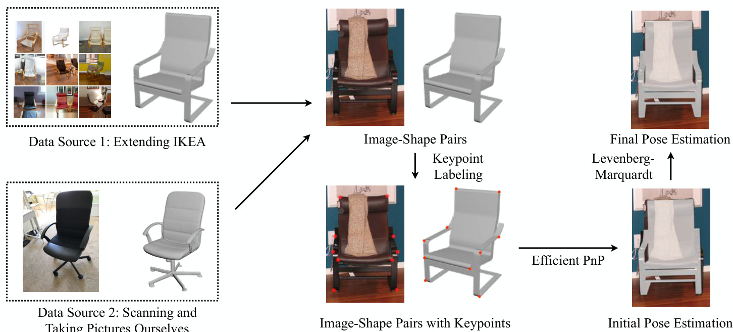
Figure 2: We build the dataset in two steps. First, we collect image-shape pairs by crawling web images of IKEA furniture as well as scanning objects and taking pictures ourselves. Second, we align the shapes with their 2D silhouettes by minimizing the 2D coordinates of the keypoints and their projected positions from 3D, using the Efficient $\mathrm{PnP}$ and the Levenberg-Marquardt algorithm.
图 2: 我们通过两个步骤构建数据集。首先,通过爬取宜家家具的网页图片、扫描实物并自行拍摄照片来收集图像-形状配对。其次,利用高效 $\mathrm{PnP}$ 和 Levenberg-Marquardt 算法,通过最小化关键点的2D坐标与其从3D投影位置的对齐误差,将形状与其2D轮廓进行匹配。
Shape retrieval. Another related research direction is retrieving similar 3D shapes given a single image, instead of reconstructing the object’s actual geometry [1, 15, 19, 49]. Pix3D contains shapes with significant inter-class and intraclass variations, and is therefore suitable for both generalpurpose and fine-grained shape retrieval tasks.
形状检索。另一个相关研究方向是根据单张图像检索相似的3D形状,而非重建物体的实际几何结构 [1, 15, 19, 49]。Pix3D数据集包含具有显著类间和类内差异的形状,因此既适用于通用检索任务,也适用于细粒度形状检索任务。
3D pose estimation. Many of the aforementioned object datasets include annotations of object poses [35, 39, 48, 64, 65]. Researchers have also proposed numerous methods on 3D pose estimation [13, 43, 56, 59]. In this paper, we show that Pix3D is also a proper benchmark for this task.
3D姿态估计。上述许多物体数据集都包含了物体姿态的标注 [35, 39, 48, 64, 65]。研究人员也提出了多种3D姿态估计方法 [13, 43, 56, 59]。本文表明,Pix3D同样是该任务的合适基准。
3. Building Pix3D
3. 构建 Pix3D
Figure 2 summarizes how we build Pix3D. We collect raw images from web search engines and shapes from 3D repositories; we also take pictures and scan shapes ourselves. Finally, we use labeled keypoints on both 2D images and 3D shapes to align them.
图 2: 总结了Pix3D的构建流程。我们从网络搜索引擎收集原始图像,从3D模型库获取形状数据;同时自行拍摄照片并扫描物体形状。最后,通过在2D图像和3D形状上标注的关键点来实现两者的对齐。
3.1. Collecting Image-Shape Pairs
3.1. 收集图像-形状对
We obtain raw image-shape pairs in two ways. One is to crawl images of IKEA furniture from the web and align them with CAD models provided in the IKEA dataset [39]. The other is to directly scan 3D shapes and take pictures.
我们通过两种方式获取原始图像-形状对。一种是从网络爬取宜家(IKEA)家具图像,并将其与IKEA数据集[39]提供的CAD模型对齐。另一种是直接扫描3D形状并拍摄照片。
images for 90 shapes. Therefore, we choose to keep the 3D shapes from IKEA dataset, but expand the set of 2D images using online image search engines and crowd sourcing.
我们选择了保留IKEA数据集中的3D形状,同时利用在线图像搜索引擎和众包来扩充2D图像集。
For each 3D shape, we first search for its corresponding 2D images through Google, Bing, and Baidu, using its IKEA model name as the keyword. We obtain 104,220 images for the 219 shapes. We then use Amazon Mechanical Turk (AMT) to remove irrelevant ones. For each image, we ask three AMT workers to label whether this image matches the 3D shape or not. For images whose three responses differ, we ask three additional workers and decide whether to keep them based on majority voting. We end up with 14,600 images for the 219 IKEA shapes.
对于每个3D形状,我们首先通过Google、Bing和百度搜索其对应的2D图像,使用其IKEA型号名称作为关键词。我们为219个形状获取了104,220张图像。随后利用Amazon Mechanical Turk (AMT) 剔除不相关图像。针对每张图像,我们请三名AMT工作人员标注该图像是否与3D形状匹配。对于三个标注结果不一致的图像,我们会额外邀请三名工作人员进行标注,并根据多数表决决定是否保留。最终我们为219个IKEA形状保留了14,600张图像。
3D scan. We scan non-IKEA objects with a Structure Sensor† mounted on an iPad. We choose to use the Structure Sensor because its mobility enables us to capture a wide range of shapes.
3D扫描。我们使用安装在iPad上的Structure Sensor†扫描非宜家物品。选择Structure Sensor是因为其便携性使我们能够捕捉各种形状。
The iPad RGB camera is synchronized with the depth sensor at $30\mathrm{Hz}$ , and calibrated by the Scanner App provided by Occipital, Inc.‡ The resolution of RGB frames is $2592\times1936$ , and the resolution of depth frames is $320\times240$ . For each object, we take a short video and fuse the depth data to get its 3D mesh by using fusion algorithm provided by Occipital, Inc. We also take 10–20 images for each scanned object in front of various backgrounds from different viewpoints, making sure the object is neither cropped nor occluded. In total, we have scanned 209 objects and taken 2,313 images. Combining these with the IKEA shapes and images, we have 418 shapes and 16,913 images altogether.
iPad的RGB摄像头与深度传感器以$30\mathrm{Hz}$频率同步,并通过Occipital公司提供的Scanner App进行校准。RGB帧的分辨率为$2592\times1936$,深度帧的分辨率为$320\times240$。对于每个物体,我们拍摄一段短视频并使用Occipital公司提供的融合算法将深度数据融合生成其3D网格。同时,我们从不同视角在各种背景前为每个扫描物体拍摄10-20张图像,确保物体未被裁剪或遮挡。总计我们扫描了209个物体并拍摄了2,313张图像。结合宜家(IKEA)的形状和图像数据,我们最终共获得418个形状和16,913张图像。
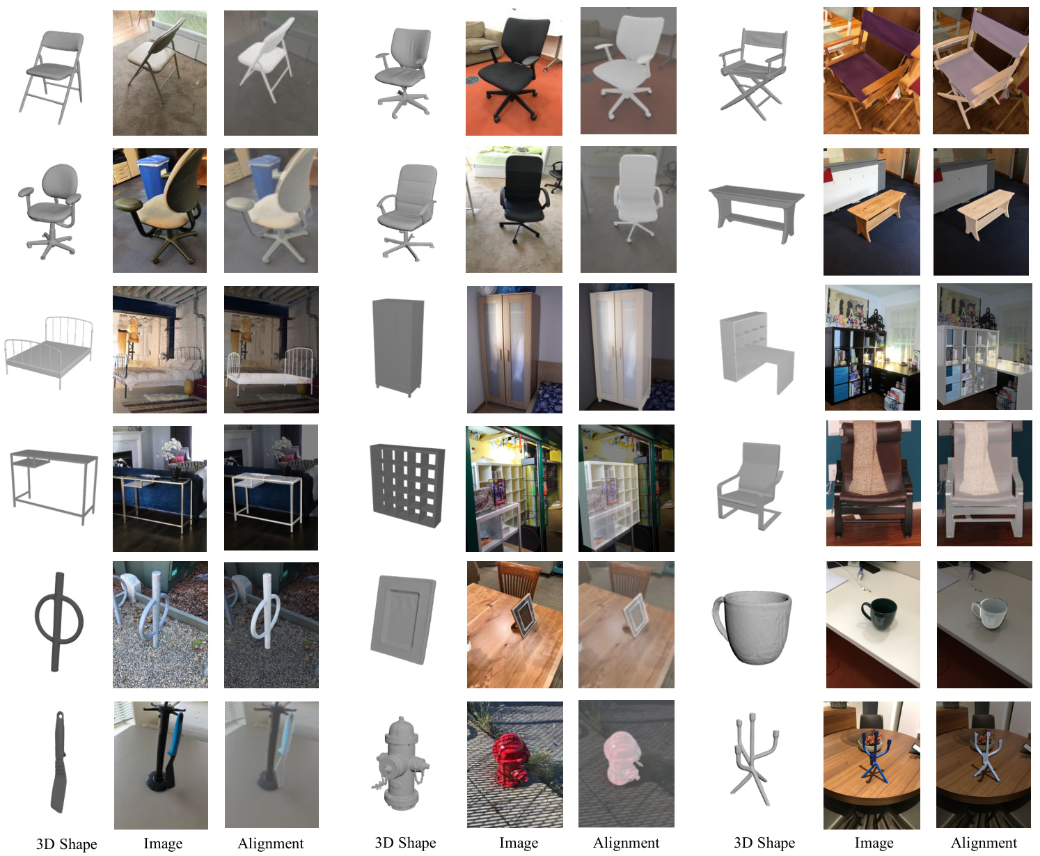
Figure 3: Sample images and shapes in Pix3D. From left to right: 3D shapes, 2D images, and 2D-3D alignment. Rows 1–2 show some chairs we scanned, rows 3–4 show a few IKEA objects, and rows 5–6 show some objects of other categories we scanned.
图 3: Pix3D中的样本图像与形状。从左至右:3D形状、2D图像及2D-3D对齐。第1-2行为我们扫描的部分椅子,第3-4行展示若干宜家(IKEA)物件,第5-6行呈现其他类别中我们扫描的物体。
3.2. Image-Shape Alignment
3.2. 图像形状对齐
To align a 3D CAD model with its projection in a 2D image, we need to solve for its 3D pose (translation and rotation), and the camera parameters used to capture the image.
为了使3D CAD模型与其在2D图像中的投影对齐,我们需要求解其3D位姿(平移和旋转)以及用于捕捉图像的相机参数。
We use a keypoint-based method inspired by Lim et al. [39]. Denote the keypoints’ 2D coordinates as $X_{\mathrm{2D}}=$ ${\mathbf{x}{1},\mathbf{x}{2},\cdots,\mathbf{x}{n}}$ and their corresponding 3D coordinates as $X_{\mathrm{3D}}={{\bf X}{1},{\bf X}{2},\cdot\cdot\cdot\mathrm{~,~}{\bf X}_{n}}$ . We solve for camera parameters and 3D poses that minimize the re projection error of the keypoints. Specifically, we want to find the projection matrix $_P$ that minimizes
我们采用了一种基于关键点的方法,灵感来源于Lim等人[39]。将关键点的2D坐标记为$X_{\mathrm{2D}}={\mathbf{x}{1},\mathbf{x}{2},\cdots,\mathbf{x}{n}}$,对应的3D坐标记为$X_{\mathrm{3D}}={{\bf X}{1},{\bf X}{2},\cdot\cdot\cdot\mathrm{~,~}{\bf X}_{n}}$。我们通过最小化关键点的重投影误差来求解相机参数和3D位姿。具体而言,需要找到使投影矩阵$_P$最小化的解。
$$
\mathcal{L}(P;X_{\mathrm{3D}},X_{\mathrm{2D}})=\sum_{i}|\mathrm{Proj}{P}(\mathbf{X}{i})-\mathbf{x}{i}|_{2}^{2},
$$
$$
\mathcal{L}(P;X_{\mathrm{3D}},X_{\mathrm{2D}})=\sum_{i}|\mathrm{Proj}{P}(\mathbf{X}{i})-\mathbf{x}{i}|_{2}^{2},
$$
where $\mathrm{Proj}_{P}(\cdot)$ is the projection function.
其中 $\mathrm{Proj}_{P}(\cdot)$ 是投影函数。
Under the central projection assumption (zero-skew, square pixel, and the optical center is at the center of the frame), we
在中心投影假设(零偏斜、方形像素且光学中心位于帧中心)下,我们
have $P=K[R|T]$ , where $\kappa$ is the camera intrinsic matrix; $\boldsymbol{R}\in\mathbb{R}^{3\times3}$ and $\pmb{T}\in\mathbb{R}^{3}$ represent the object’s 3D rotation and 3D translation, respectively. We know
有 $P=K[R|T]$,其中 $\kappa$ 是相机内参矩阵;$\boldsymbol{R}\in\mathbb{R}^{3\times3}$ 和 $\pmb{T}\in\mathbb{R}^{3}$ 分别表示物体的三维旋转和三维平移。已知
$$
K=\left[{\begin{array}{c c c}{f}&{0}&{w/2}\ {0}&{f}&{h/2}\ {0}&{0}&{1}\end{array}}\right],
$$
$$
K=\left[{\begin{array}{c c c}{f}&{0}&{w/2}\ {0}&{f}&{h/2}\ {0}&{0}&{1}\end{array}}\right],
$$
where $f$ is the focal length, and $w$ and $h$ are the width and height of the image. Therefore, there are altogether seven parameters to be estimated: rotations $\theta,\phi,\psi$ , translations $x,y,z$ , and focal length $f$ (Rotation matrix $R$ is determined by $\theta,\phi$ , and $\psi$ ).
其中 $f$ 为焦距,$w$ 和 $h$ 分别为图像的宽度和高度。因此,共有七个待估计参数:旋转角度 $\theta,\phi,\psi$、平移量 $x,y,z$ 以及焦距 $f$(旋转矩阵 $R$ 由 $\theta,\phi$ 和 $\psi$ 确定)。
To solve Equation 1, we first calculate a rough 3D pose using the Efficient $\mathrm{P}n\mathrm{P}$ algorithm [36] and then refine it using the Levenberg-Marquardt algorithm [37, 40], as shown in Figure 2. Details of each step are described below.
为求解方程1,我们首先使用高效的 $\mathrm{P}n\mathrm{P}$ 算法 [36] 计算粗略的3D姿态,然后利用Levenberg-Marquardt算法 [37, 40] 进行优化,如图2所示。各步骤细节如下所述。
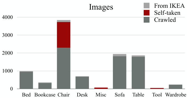
Figure 4: The distribution of images across categories
图 4: 各类别图像分布情况
Efficient $\mathbf{P}\pmb{n}\mathbf{P}.$ Perspective $\cdot n$ -Point $({\mathrm{P}}n{\mathrm{P}})$ is the problem of estimating the pose of a calibrated camera given paired 3D points and 2D projections. The Efficient $\mathrm{P}n\mathrm{P}$ (EPnP) algorithm solves the problem using virtual control points [37]. Because EPnP does not estimate the focal length, we enumerate the focal length $f$ from 300 to 2,000 with a step size of 10, solve for the 3D pose with each $f$ , and choose the one with the minimum projection error.
高效 $\mathbf{P}\pmb{n}\mathbf{P}.$ 透视 $\cdot n$ 点 $({\mathrm{P}}n{\mathrm{P}})$ 问题是在给定配对3D点和2D投影的情况下估计校准相机的姿态。高效 $\mathrm{P}n\mathrm{P}$ (EPnP) 算法通过虚拟控制点解决该问题 [37]。由于EPnP不估算焦距,我们以10为步长枚举300至2,000范围内的焦距 $f$,为每个 $f$ 求解3D姿态,并选择投影误差最小的结果。
The Levenberg-Marquardt algorithm (LMA). We take the output of $\mathrm{EPnP}$ with 50 random disturbances as the initial states, and run LMA on each of them. Finally, we choose the solution with the minimum projection error.
Levenberg-Marquardt算法 (LMA)。我们将带有50次随机扰动的$\mathrm{EPnP}$输出作为初始状态,并对每个状态运行LMA。最终选择具有最小投影误差的解。
Implementation details. For each 3D shape, we manually label its 3D keypoints. The number of keypoints ranges from 8 to 24. For each image, we ask three AMT workers to label if each keypoint is visible on the image, and if so, where it is. We only consider visible keypoints during the optimization.
实现细节。对于每个3D形状,我们手动标注其3D关键点,关键点数量为8到24个不等。针对每张图像,我们聘请三名AMT工作人员标注各关键点是否在图像中可见,若可见则标注其位置。优化过程中仅考虑可见关键点。
The 2D keypoint annotations are noisy, which severely hurts the performance of the optimization algorithm. We try two methods to increase its robustness. The first is to use RANSAC. The second is to use only a subset of 2D keypoint annotations. For each image, denote $C={c_{1},c_{2},c_{3}}$ as its three sets of human annotations. We then enumerate the seven nonempty subsets $C_{k}\subseteq C$ ; for each keypoint, we compute the median of its 2D coordinates in $C_{k}$ . We apply our optimization algorithm on every subset $C_{k}$ , and keep the output with the minimum projection error. After that, we let three AMT workers choose, for each image, which of the two methods offers better alignment, or neither performs well. At the same time, we also collect attributes (i.e., truncation, occlusion) for each image. Finally, we fine-tune the annotations ourselves using the GUI offered in Object Net 3 D [64]. Altogether there are 395 3D shapes and 10,069 images. Sample 2D-3D pairs are shown in Figure 3.
2D关键点标注存在噪声,这会严重损害优化算法的性能。我们尝试了两种方法来提高其鲁棒性。第一种是使用RANSAC。第二种是仅使用2D关键点标注的子集。对于每张图像,记 $C={c_{1},c_{2},c_{3}}$ 为其三组人工标注。然后我们枚举七个非空子集 $C_{k}\subseteq C$;对于每个关键点,我们计算其在 $C_{k}$ 中2D坐标的中位数。我们在每个子集 $C_{k}$ 上应用优化算法,并保留投影误差最小的输出。之后,我们让三位AMT工作人员为每张图像选择两种方法中哪一种对齐效果更好,或者两者效果都不佳。同时,我们还为每张图像收集了属性(即截断、遮挡)。最后,我们使用Object Net 3D [64]提供的GUI自行微调标注。总共有395个3D形状和10,069张图像。示例2D-3D对如图3所示。
4. Exploring Pix3D
4. Pix3D探索
We now present some statistics of Pix3D, and contrast it with its predecessors.
我们现在展示Pix3D的一些统计数据,并与之前的数据集进行对比。
Dataset statistics. Figures 4 and 5 show the category distributions of 2D images and 3D shapes in Pix3D; Figure 6 shows the distribution of the number of images each model has. Our dataset covers a large variety of shapes, each of which has a large number of in-the-wild images. Chairs cover the significant part of Pix3D, because they are common, highly diverse, and well-studied by recent literature [11, 60, 20].
数据集统计。图4和图5展示了Pix3D中2D图像和3D形状的类别分布;图6显示了每个模型对应的图像数量分布。我们的数据集涵盖了多种形状,每种形状都包含大量真实场景图像。椅子在Pix3D中占比较大,因为它们常见、多样性高,且被近期研究广泛关注 [11, 60, 20]。
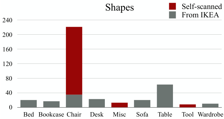
Figure 5: The distribution of shapes across categories
图 5: 各类别形状分布
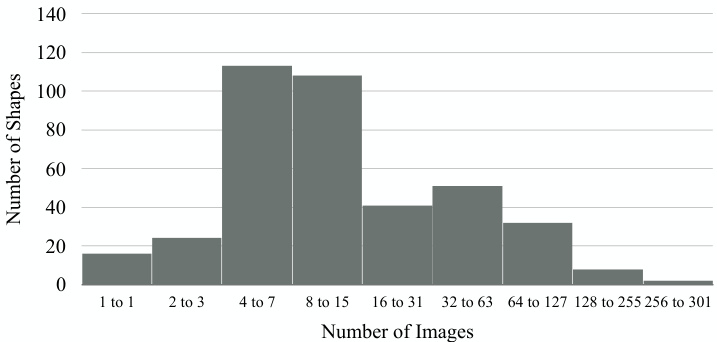
Figure 6: Number of images available for each shape
图 6: 每种形状可用的图像数量
Quantitative evaluation. As a quantitative comparison on the quality of Pix3D and other datasets, we randomly select 25 chair and 25 sofa images from PASCAL $^{3\mathrm{D}+}$ [65], ObjectNet3D [64], IKEA [39], and Pix3D. For each image, we render the projected 2D silhouette of the shape using its pose annotation provided by the dataset. We then manually annotate the ground truth object masks in these images, and calculate Intersection over Union (IoU) between the projections and the ground truth. For each image-shape pair, we also ask 50 AMT workers whether they think the image is picturing the 3D ground truth shape provided by the dataset.
定量评估。为了定量比较Pix3D与其他数据集的质量,我们从PASCAL $^{3\mathrm{D}+}$ [65]、ObjectNet3D [64]、IKEA [39]和Pix3D中随机选取25张椅子和25张沙发的图像。对于每张图像,我们利用数据集提供的姿态标注渲染形状的投影2D轮廓,并人工标注这些图像中的真实物体掩膜,计算投影与真实掩膜的交并比(IoU)。针对每张图像-形状组合,我们还邀请了50名AMT工作人员判断该图像是否呈现了数据集提供的3D真实形状。
From Table 1, we see that Pix3D has much higher IoUs than PASCAL $^{3\mathrm{D}+}$ and Object Net 3 D, and slightly higher IoUs compared with the IKEA dataset. Humans also feel IKEA and $\mathrm{Pix}3\mathrm{D}$ have matched images and shapes, but not PASCAL $^{3\mathrm{D}+}$ or Object Net 3 D. In addition, we observe that many CAD models in the IKEA dataset are of an incorrect scale, making it challenging to align the shapes with images. For example, there are only 15 unoccluded and un truncated images of sofas in IKEA, while Pix3D has 1,092.
从表1可以看出,Pix3D的IoU值显著高于PASCAL $^{3\mathrm{D}+}$ 和Object Net 3D,相较IKEA数据集也略胜一筹。人类评估者也认为IKEA和$\mathrm{Pix}3\mathrm{D}$的图像与形状匹配度较高,而PASCAL $^{3\mathrm{D}+}$和Object Net 3D则不尽如人意。此外,我们注意到IKEA数据集中许多CAD模型比例失准,导致形状与图像对齐困难。例如IKEA仅有15张无遮挡且完整的沙发图像,而Pix3D则包含1,092张。
5. Metrics
5. 指标
Designing a good evaluation metric is important to encourage researchers to design algorithms that reconstruct highquality 3D geometry, rather than low-quality 3D reconstruction that overfits to a certain metric.
设计一个好的评估指标对于鼓励研究人员设计能够重建高质量3D几何的算法非常重要,而不是过度拟合某一特定指标的低质量3D重建。
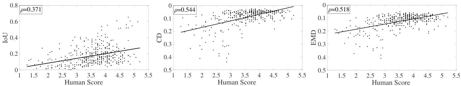
Figure 7: Scatter plots between humans’ ratings of reconstructed shapes and their IoU, CD, and EMD. The three metrics have a Pearson’s coefficient of 0.371, 0.544, and 0.518, respectively.
图 7: 人类对重建形状评分与其IoU (Intersection over Union) 、CD (Chamfer Distance) 和EMD (Earth Mover's Distance) 的散点图。这三个指标的皮尔逊相关系数分别为0.371、0.544和0.518。
Table 1: We compute the Intersection over Union (IoU) between manually annotated 2D masks and the 2D projections of 3D shapes. We also ask humans to judge whether the object in the images matches the provided shape.
表 1: 我们计算了人工标注的2D掩码与3D形状的2D投影之间的交并比(IoU)。同时邀请人类评估者判断图像中的物体是否与提供的形状匹配。
Many 3D reconstruction papers use Intersection over Union (IoU) to evaluate the similarity between ground truth and reconstructed 3D voxels, which may significantly deviate from human perception. In contrast, metrics like shortest distance and geodesic distance are more commonly used than IoU for matching meshes in graphics [32, 25]. Here, we conduct behavioral studies to calibrate IoU, Chamfer distance (CD) [2], and Earth Mover’s distance (EMD) [46] on how well they reflect human perception.
许多3D重建论文使用交并比(IoU)来评估真实3D体素与重建结果之间的相似度,但该指标可能与人类感知存在显著偏差。相比之下,在图形学领域中[32, 25],最短距离和测地线距离等指标比IoU更常用于网格匹配。我们通过行为研究来校准IoU、倒角距离(CD) [2]和推土机距离(EMD) [46]与人类感知的吻合程度。
5.1. Definitions
5.1. 定义
The definition of IoU is straightforward. For Chamfer distance (CD) and Earth Mover’s distance (EMD), we first convert voxels to point clouds, and then compute CD and EMD between pairs of point clouds.
IoU的定义很直观。对于倒角距离 (Chamfer distance, CD) 和推土机距离 (Earth Mover's distance, EMD),我们首先将体素转换为点云,然后计算点云对之间的CD和EMD。
| Chairs | Sofas | |||
| IoU | Match? | IoU | Match? | |
| PASCAL 3D+ [65] | 0.514 | 0.00 | 0.813 | 0.00 |
| ObjectNet3D [64] | 0.570 | 0.16 | 0.773 | 0.08 |
| IKEA [39] | 0.748 | 1.00 | 0.918 | 1.00 |
| Pix3D (ours) | 0.835 | 1.00 | 0.926 | 1.00 |
Table 2: Spearman’s rank correlation coefficients between different metrics. IoU, EMD, and CD have a correlation coefficient of 0.32, 0.43, and 0.49 with human judgments, respectively.
| 椅子 | 沙发 | |||
|---|---|---|---|---|
| IoU | 匹配? | IoU | 匹配? | |
| PASCAL 3D+ [65] | 0.514 | 0.00 | 0.813 | 0.00 |
| ObjectNet3D [64] | 0.570 | 0.16 | 0.773 | 0.08 |
| IKEA [39] | 0.748 | 1.00 | 0.918 | 1.00 |
| Pix3D (本工作) | 0.835 | 1.00 | 0.926 | 1.00 |
表 2: 不同指标间的Spearman等级相关系数。IoU、EMD和CD与人类判断的相关系数分别为0.32、0.43和0.49。
Voxels to a point cloud. We first extract the isosurface of each predicted voxel using the Lewiner marching cubes [38] algorithm. In practice, we use 0.1 as a universal surface value for extraction. We then uniformly sample points on the surface meshes and create the densely sampled point clouds. Finally, we randomly sample 1,024 points from each point cloud and normalize them into a unit cube for distance calculation.
体素到点云。我们首先使用Lewiner移动立方体[38]算法提取每个预测体素的等值面。实际操作中,我们采用0.1作为通用的表面提取阈值。接着在表面网格上均匀采样点,生成密集采样的点云。最后,我们从每个点云中随机采样1,024个点,并将其归一化至单位立方体内以进行距离计算。
Chamfer distance (CD). The Chamfer distance (CD) between $S_{1},S_{2}\subseteq\mathbb{R}^{3}$ is defined as
倒角距离 (CD)。倒角距离 (CD) 用于衡量 $S_{1},S_{2}\subseteq\mathbb{R}^{3}$ 两个点集之间的差异,其定义为
$$
\mathrm{CD}(S_{1},S_{2})={\frac{1}{|S_{1}|}}\sum_{x\in S_{1}}{\underset{y\in S_{2}}{\mathrm{min}}}|x-y|{2}+{\frac{1}{|S_{2}|}}\sum_{y\in S_{2}}{\underset{x\in S_{1}}{\mathrm{min}}}|x-y|_{2}.
$$
$$
\mathrm{CD}(S_{1},S_{2})={\frac{1}{|S_{1}|}}\sum_{x\in S_{1}}{\underset{y\in S_{2}}{\mathrm{min}}}|x-y|{2}+{\frac{1}{|S_{2}|}}\sum_{y\in S_{2}}{\underset{x\in S_{1}}{\mathrm{min}}}|x-y|_{2}.
$$
For each point in each cloud, CD finds the nearest point in the other point set, and sums the distances up. CD has been used in recent shape retrieval challenges [68].
对于每个点云中的每个点,CD (Chamfer Distance) 会在另一个点集中找到最近的点,并将这些距离求和。CD 已被用于近期的形状检索挑战赛 [68]。
| IoU | EMD | CD | Human | |
|---|---|---|---|---|
| IoU | 1 | 0.55 | 0.60 | 0.32 |
| EMD | 0.55 | 1 | 0.78 | 0.43 |
| CD | 0.60 | 0.78 | 1 | 0.49 |
| Human | 0.32 | 0.43 | 0.49 | 1 |
Earth Mover’s distance (EMD). We follow the definition of EMD in Fan et al. [12]. The Earth Mover’s distance (EMD) between $S_{1},S_{2}\subseteq\mathbb{R}^{3}$ (of equal size, i.e., $|S_{1}|=|S_{2}|)$ is
推土机距离 (Earth Mover's Distance, EMD)。我们沿用Fan等人[12]对EMD的定义。对于等规模点集$S_{1},S_{2}\subseteq\mathbb{R}^{3}$ (即满足$|S_{1}|=|S_{2}|)$,其推土机距离定义为
$$
\operatorname{EMD}(S_{1},S_{2})={\frac{1}{|S_{1}|}}\operatorname*{min}{\phi:S_{1}\to S_{2}}\sum_{x\in S_{1}}|x-\phi(x)|_{2},
$$
$$
\operatorname{EMD}(S_{1},S_{2})={\frac{1}{|S_{1}|}}\operatorname*{min}{\phi:S_{1}\to S_{2}}\sum_{x\in S_{1}}|x-\phi(x)|_{2},
$$
where $\phi:S_{1}\rightarrow S_{2}$ is a bijection. We divide EMD by the size of the point cloud for normalization. In practice, calculating the exact EMD value is computationally expensive; we instead use a $(1+\epsilon)$ approximation algorithm [3].
其中 $\phi:S_{1}\rightarrow S_{2}$ 是一个双射。我们将 EMD 除以点云大小以实现归一化。实际计算中,精确计算 EMD 值的计算成本很高;我们转而使用 $(1+\epsilon)$ 近似算法 [3]。
5.2. Experiments
5.2. 实验
We then conduct two user studies to compare these metrics and benchmark how they capture human perception.
我们随后进行了两项用户研究,以比较这些指标并评估它们如何捕捉人类感知。
Which one looks better? We run three shape reconstructions algorithms (3D-R2N2 [9], DRC [60], and 3D-VAEGAN [63]) on 200 randomly selected images of chairs. We then, for each image and every pair of its three constructions, ask three AMT workers to choose the one that looks closer to the object in the image. We also compute how each pair of objects rank in each metric. Finally, we calculate the Spearman’s rank correlation coefficients between different metrics (i.e., IoU, EMD, CD, and human perception). Table 2 suggests that EMD and CD correlate better with human ratings.
哪个看起来更好?我们在200张随机选择的椅子图像上运行了三种形状重建算法(3D-R2N2 [9]、DRC [60]和3D-VAEGAN [63])。然后,针对每张图像及其三个重建结果中的每一对,我们请三位AMT工作者选择看起来更接近图像中物体的那个。我们还计算了每对物体在每个指标中的排名。最后,我们计算了不同指标(即IoU、EMD、CD和人类感知)之间的斯皮尔曼等级相关系数。表2表明,EMD和CD与人类评分相关性更好。
How good is it? We randomly select 400 images, and show each of them to 15 AMT workers, together with the voxel prediction by DRC [60] and the ground truth shape. We then ask them to rate the reconstruction, on a scale of 1 to 7, based on how similar it is to the ground truth. The scatter plot in Figure 7 suggests that CD and EMD have higher Pearson’s coefficients with human responses.
效果如何?我们随机选取400张图像,每张图像展示给15名AMT工作人员,同时提供DRC [60]的体素预测结果和真实形状。随后要求他们根据重建结果与真实形状的相似度,以1到7分为标准进行评分。图7中的散点图显示,CD和EMD与人类反馈的皮尔逊相关系数更高。
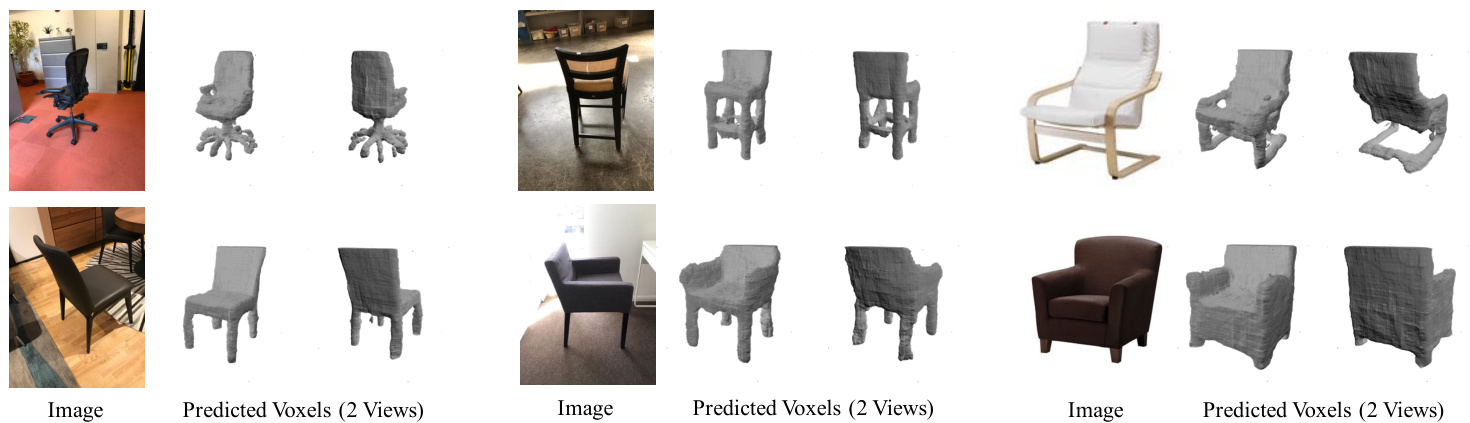
Figure 8: Results on 3D reconstructions of chairs. We show two views of the predicted voxels for each example.
图 8: 椅子三维重建结果。我们为每个示例展示预测体素的两个视角视图。
| IoU | EMD | CD | |
|---|---|---|---|
| 3D-R2N2 [9] | 0.136 | 0.211 | 0.239 |
| PSGN [12] | N/A | 0.216 | 0.200 |
| 3D-VAE-GAN [63] | 0.171 | 0.176 | 0.182 |
| DRC [60] | 0.265 | 0.144 | 0.160 |
| MarrNet* [61] | 0.231 | 0.136 | 0.144 |
| AtlasNet[18] | N/A | 0.128 | 0.125 |
| Ours (w/oPose) | 0.267 | 0.124 | 0.124 |
| Ours (w/ Pose) | 0.282 | 0.118 | 0.119 |
Table 3: Results on 3D shape reconstruction. Our model gets the highest IoU, EMD, and CD. We also compare our full model with a variant that does not have the view estimator. Results show that multi-task learning helps boost its performance. As MarrNet and PSGN predict viewer-centered shapes, while the other methods are object-centered, we rotate their reconstructions into the canonical view using ground truth pose annotations before evaluation.
表 3: 三维形状重建结果。我们的模型在 IoU、EMD 和 CD 指标上均取得最高值。同时对比了完整模型与无视角估计器变体的性能,结果表明多任务学习能有效提升表现。由于 MarrNet 和 PSGN 预测的是以观察者为中心的形状,而其他方法均为以物体为中心,因此在评估前我们使用真实位姿标注将其重建结果旋转至标准视角。
6. Approach
6. 方法
Pix3D serves as a benchmark for shape modeling tasks including reconstruction, retrieval, and pose estimation. Here, we design a new model that simultaneously performs shape reconstruction and pose estimation, and evaluate it on Pix3D.
Pix3D作为形状建模任务的基准,包括重建、检索和姿态估计。在此,我们设计了一个同时执行形状重建和姿态估计的新模型,并在Pix3D上进行了评估。
Our model is an extension of MarrNet [61], both of which use 2.5D sketches (the object’s depth, surface normals, and silhouette) as an intermediate representation. It contains four modules: (1) a 2.5D sketch estimator that predicts the depth, surface normals, and silhouette of the object; (2) a 2.5D sketch encoder that encodes the 2.5D sketches into a lowdimensional latent vector; (3) a 3D shape decoder and (4) a view estimator that decodes a latent vector into a 3D shape and camera parameters, respectively. Different from MarrNet [61], our model has an additional branch for pose estimation. We briefly describe them below, and please refer to the supplementary material for more details.
我们的模型是对 MarrNet [61] 的扩展,两者都使用 2.5D 草图(物体的深度、表面法线和轮廓)作为中间表示。它包含四个模块:(1) 用于预测物体深度、表面法线和轮廓的 2.5D 草图估计器;(2) 将 2.5D 草图编码为低维潜在向量的 2.5D 草图编码器;(3) 3D 形状解码器;(4) 将潜在向量分别解码为 3D 形状和相机参数的视角估计器。与 MarrNet [61] 不同,我们的模型增加了姿态估计分支。下文将简要描述这些模块,更多细节请参阅补充材料。
2.5D sketch estimator. The first module takes an RGB image as input and predicts the object’s 2.5D sketches (its depth, surface normals, and silhouette). We use an encoder-decoder network. The encoder is based on a ResNet-18 [22] and turns a $256\times256$ image into 384 feature maps of size $16\times16$ ; the decoder has three branches for depth, surface normals, and silhouette, respectively, each consisting of four sets of $5\times5$ transposed convolutional, batch normalization and ReLU layers, followed by one $5\times5$ convolutional layer. All output sketches are of size $256\times256$ .
2.5D草图估计器。第一个模块以RGB图像作为输入,预测物体的2.5D草图(包括深度、表面法线和轮廓)。我们采用编码器-解码器网络架构:编码器基于ResNet-18 [22],将$256×256$图像转换为384个$16×16$大小的特征图;解码器包含深度、表面法线和轮廓三个分支,每个分支由四组$5×5$转置卷积层、批量归一化层和ReLU层构成,最后接一个$5×5$卷积层。所有输出草图尺寸均为$256×256$。
2.5D sketch encoder. We use a modified ResNet-18 [22] that takes a four-channel image (three for surface normals and one for depth). Each channel is masked by the predicted silhouette. A final linear layer outputs a 200-D latent vector.
2.5D草图编码器。我们使用改进的ResNet-18 [22],它接收四通道图像(三个用于表面法线,一个用于深度)。每个通道通过预测的轮廓进行掩码处理。最终的线性层输出一个200维的潜在向量。
3D shape decoder. Our 3D shape decoder has five sets of $4\times4\times4$ transposed convolutional, batch-norm, and ReLU layers, followed by a $4\times4\times4$ transposed convolutional layer. It outputs a voxelized shape of size $128\times128\times128$ in the object’s canonical view.
3D形状解码器。我们的3D形状解码器包含五组$4\times4\times4$转置卷积、批量归一化和ReLU层,随后接一个$4\times4\times4$转置卷积层。它输出物体规范视角下尺寸为$128\times128\times128$的体素化形状。
View estimator. The view estimator contains three sets of linear, batch normalization, and ReLU layers, followed by two parallel linear and softmax layers that predict the shape’s azimuth and elevation, respectively. Here, we treat pose estimation as a classification problem, where the 360-degree azimuth angle is divided into 24 bins and the 180-degree elevation angle is divided into 12 bins.
视角估计器。视角估计器包含三组线性层、批归一化层和ReLU层,后接两个并行的线性层和softmax层,分别预测形状的方位角和仰角。此处我们将姿态估计视为分类问题,其中360度方位角被划分为24个区间,180度仰角被划分为12个区间。
Training paradigm. For training, we use Mitsuba [26] to render each chair in ShapeNet [7] from 20 random views using three types of backgrounds: 1/3 on a white background, 1/3 on high-dynamic-range backgrounds with illumination channels, and 1/3 on backgrounds randomly sampled from the SUN database [66]. We augment our training data by random color and light jittering.
训练范式。在训练过程中,我们使用Mitsuba [26]从20个随机视角渲染ShapeNet [7]中的每把椅子,并采用三种背景类型:1/3为纯白背景,1/3为带光照通道的高动态范围(HDR)背景,1/3为从SUN数据库[66]随机采样的背景。通过随机颜色和光照抖动对训练数据进行增强。
We first train the 2.5D sketch estimator. We then train the 2.5D sketch encoder and the 3D shape decoder (and the view estimator if we’re predicting the pose) jointly. We finally concatenate them for prediction.
我们首先训练2.5D草图估计器。接着联合训练2.5D草图编码器和3D形状解码器(若需预测姿态则同时训练视角估计器)。最后将它们拼接以进行预测。
7. Experiments
7. 实验
We now evaluate our model and state-of-the-art algorithms on single-image 3D shape reconstruction, retrieval, and pose estimation, all using Pix3D. For all experiments, we use the 2,894 un truncated and unoccluded chair images.
我们现在使用Pix3D数据集评估我们的模型和最先进算法在单图像3D形状重建、检索和姿态估计任务上的表现。所有实验均采用2,894张未经裁剪且无遮挡的椅子图像。
3D shape reconstruction. We compare our model, with and without the pose estimation branch, with the state-ofthe-art systems, including 3D-VAE-GAN [63], 3D-R2N2 [9],
3D形状重建。我们将带姿态估计分支和不带姿态估计分支的模型与当前最先进的系统进行比较,包括3D-VAE-GAN [63]、3D-R2N2 [9]。

Top-8 Retrieval Results
图 1: 前8个检索结果
Figure 9: Results on shape retrieval. We show the top-8 retrieval results from our proposed method (with and without pose estimation). The variant with pose estimation tends to retrieve images of shapes in a similar pose.
图 9: 形状检索结果。我们展示了所提方法(带姿态估计和不带姿态估计的变体)的Top-8检索结果。带姿态估计的变体倾向于检索姿态相似的形状图像。

Figure 10: Results on pose estimation. Our method predicts azimuth and elevation accurately.
Table 5: Results on 3D pose estimation. Our model outperforms Render for CNN [56] in both azimuth and elevation.
图 10: 姿态估计结果。我们的方法能准确预测方位角和仰角。
| R@1 | R@2 | R@4 | R@8 | R@16 | R@32 |
|---|---|---|---|---|---|
| 3D-VAE-GAN[63] | 0.02 | 0.03 | 0.07 | 0.12 | 0.21 |
| MarrNet[61] | 0.42 | 0.51 | 0.57 | 0.64 | 0.71 |
| Ours (w/Pose) | 0.42 | 0.48 | 0.55 | 0.63 | 0.70 |
| Ours (w/oPose) | 0.53 | 0.62 | 0.71 | 0.78 | 0.85 |
表 5: 三维姿态估计结果。我们的模型在方位角和仰角预测上均优于Render for CNN[56]。
Table 4: Results on image-based shape retrieval, where $\mathbb{R}\ @\mathbb{K}$ stands for Recall $\ @\mathrm{K}$ . Our model (without the pose estimation module) achieves the highest numbers. Our model (with the pose estimation module) does not perform as well, because it sometimes retrieves images of objects with the same pose, but not exactly the same shape.
表 4: 基于图像的形状检索结果,其中 $\mathbb{R}\ @\mathbb{K}$ 表示 Recall $\ @\mathrm{K}$。我们的模型(不带姿态估计模块)取得了最高分数。我们的模型(带姿态估计模块)表现稍逊,因为它有时会检索到姿态相同但形状不完全相同的物体图像。
DRC [60], and MarrNet [61]. We use pre-trained models offered by the authors and we crop the input images as required by each algorithm. The results are shown in Table 3 and Figure 8. Our model outperforms the state-of-the-arts in all metrics. Our full model gets better results compared with the variant without the view estimator, suggesting multi-task learning helps to boost its performance. Also note the discrepancy among metrics: MarrNet has a lower IoU than DRC, but according to EMD and CD, it performs better.
DRC [60] 和 MarrNet [61]。我们使用作者提供的预训练模型,并根据各算法要求对输入图像进行裁剪。结果如表 3 和图 8 所示。我们的模型在所有指标上均优于现有最优方法。完整模型相比未配备视角估计器的变体取得了更好结果,表明多任务学习有助于提升性能。还需注意指标间的差异:MarrNet 的 IoU 低于 DRC,但根据 EMD 和 CD 指标,其表现更优。
Image-based, fine-grained shape retrieval. For shape retrieval, we compare our model with 3D-VAE-GAN [63] and MarrNet [61]. We use the latent vector from each algorithm as its embedding of the input image, and use L2 distance for image retrieval. For each test image, we retrieve its K nearest neighbors from the test set, and use Recall $\ @\mathrm{K}$ [28] to compute how many retrieved images are actually depicting the same shape. Here we do not consider images whose shape is not captured by any other images in the test set. The results are shown in Table 4 and Figure 9. Our model (without the pose estimation module) achieves the highest numbers; our model (with the pose estimation module) does not perform as well, because it sometimes retrieves images of objects with the same pose, but not exactly the same shape.
基于图像的细粒度形状检索。在形状检索任务中,我们将本模型与3D-VAE-GAN [63]和MarrNet [61]进行对比。使用各算法生成的潜向量作为输入图像的嵌入表示,并采用L2距离进行图像检索。对于每个测试图像,我们从测试集中检索其K个最近邻,并通过召回率$\ @\mathrm{K}$ [28]计算实际描绘相同形状的检索图像比例(测试集中未被其他图像捕获的形状不计入统计)。结果如表4和图9所示:未搭载位姿估计模块的本模型取得最优结果;而搭载位姿估计模块的版本因偶尔会检索到相同位姿但非完全一致形状的对象图像,表现稍逊。
| #ofviews | Azimuth | Elevation | ||||
|---|---|---|---|---|---|---|
| 4 | 8 | 12 | 4 | 6 | 12 | |
| Render for CNN Ours | 0.71 0.76 | 0.63 0.73 | 0.56 0.40 0.61 0.49 | 0.57 0.87 | 0.56 0.70 | 0.37 |
3D pose estimation. We compare our method with Render for CNN [56]. We calculate the classification accuracy for both azimuth and elevation, where the azimuth is divided into 24 bins and the elevation into 12 bins. Table 5 suggests that our model outperforms Render for CNN in pose estimation. Qualitative results are included in Figure 10.
3D姿态估计。我们将本方法与Render for CNN [56]进行对比,分别计算方位角和仰角的分类准确率,其中方位角划分为24个区间,仰角划分为12个区间。表5显示我们的模型在姿态估计任务上优于Render for CNN,定性结果如图10所示。
8. Conclusion
8. 结论
We have presented Pix3D, a large-scale dataset of wellaligned 2D images and 3D shapes. We have also explored how three commonly used metrics correspond to human perception through two behavioral studies and proposed a new model that simultaneously performs shape reconstruction and pose estimation. Experiments showed that our model achieved state-of-the-art performance on 3D reconstruction, shape retrieval, and pose estimation. We hope our paper will inspire future research in single-image 3D shape modeling.
我们提出了Pix3D——一个大规模且对齐良好的2D图像与3D形状数据集。通过两项行为研究,我们探究了三种常用指标与人类感知的对应关系,并提出了一种同时执行形状重建与姿态估计的新模型。实验表明,该模型在3D重建、形状检索和姿态估计任务上均达到了最先进性能。我们希望本文能启发单图像3D形状建模领域的未来研究。
Acknowledgements. This work is supported by NSF #1212849 and #1447476, ONR MURI N00014-16-1-2007, the Center for Brain, Minds and Machines (NSF STC award CCF-1231216), the Toyota Research Institute, and Shell Research. J. Wu is supported by a Facebook fellowship.
致谢。本研究由美国国家科学基金会(NSF #1212849和#1447476)、海军研究办公室多学科大学研究计划(MURI N00014-16-1-2007)、大脑心智与机器中心(NSF STC资助CCF-1231216)、丰田研究院以及壳牌研究公司资助。J. Wu的研究工作获得Facebook奖学金支持。
References
参考文献

Figure 11: Our model has four major components: (a) a 2.5D sketch estimator, (b) a 2.5D sketch encoder, (c) a 3D shape decoder, and (d) a view estimator. Our model first predicts 2.5D sketches from an RGB image. It then encodes the 2.5D sketches into a latent vector. Finally, a 3D shape is decoded from the 3D shape decoder, and azimuth and elevation are estimated by the view estimator.
图 11: 我们的模型包含四个主要组件: (a) 2.5D草图估计器, (b) 2.5D草图编码器, (c) 3D形状解码器, 以及 (d) 视角估计器。该模型首先从RGB图像预测2.5D草图, 然后将2.5D草图编码为潜在向量, 最后由3D形状解码器解码出3D形状, 并通过视角估计器预测方位角和仰角。
Table 6: The architecture of our 2.5D sketch estimator
表 6: 我们的2.5D草图估计器架构
| Type | Configurations |
|---|---|
| ResNet-18 [22] deconv | 不包含最后两层 (avg pool 和 fc) |
| batchnorm | 映射数: 512到384, 卷积核: 5x5, 步长: 2, 填充: 2 |
| deconv relu deconv | |
| batchnorm batchnorm batchnorm | 映射数: 384到384, 卷积核: 5x5, 步长: 2, 填充: 2 |
| relu relu relu | |
| deconv deconv deconv | 映射数: 384到384, 卷积核: 5x5, 步长: 2, 填充: 2 |
| batchnorm batchnorm batchnorm | |
| relu relu relu | |
| deconv deconv deconv | 映射数: 384到192, 卷积核: 5x5, 步长: 2, 填充: 2 |
| batchnorm batchnorm batchnorm | |
| relu relu relu | |
| deconv deconv deconv | 映射数: 192到96, 卷积核: 5x5, 步长: 2, 填充: 2 |
| batchnorm batchnorm batchnorm | |
| relu relu relu | |
| conv conv | |
| conv | 映射数: 96到3 (法线) / 到1 (其他), 卷积核: 5x5, 步长: 1, 填充: 2 |
A. Network Parameters
A. 网络参数
As mentioned in Section 6 in the main text, we proposed a new model that simultaneously performs 3D shape reconstruction and camera view estimation. Here we provide more details about the network structure.
如正文第6节所述,我们提出了一种同时进行3D形状重建和相机视角估计的新模型。此处将提供更多关于网络结构的细节。
As shown in Figure 11, our model consists of four components: (1) a 2.5D sketch estimator, which estimates 2.5D sketches from an RGB image, (2) a 2.5D sketch encoder, which encodes 2.5D sketches into a 200-dimensional latent vector, (3) a 3D shape decoder, which decodes a latent vector into voxels and (4) a view estimator, which estimates the camera view from a latent vector.
如图 11 所示,我们的模型包含四个组件:(1) 2.5D 草图估计器,用于从 RGB 图像估计 2.5D 草图,(2) 2.5D 草图编码器,将 2.5D 草图编码为 200 维潜在向量,(3) 3D 形状解码器,将潜在向量解码为体素,(4) 视角估计器,从潜在向量估计相机视角。
2.5D sketch estimator. Table 6 shows the network configuration summary of the 2.5D sketch estimator. We use an encoder-decoder network. The first four rows in Table 6 shows the encoder’s structure and the other rows describe the decoder. The encoder takes in an input RGB image of size $256\times256$ and encodes it into $384 16\times16$ feature maps. The decoder takes in $384~16\times16$ feature maps and decodes them into the object’s surface normals, depth, and silhouette of size $256\times256$ .
2.5D草图估算器。表6展示了2.5D草图估算器的网络配置摘要。我们采用编码器-解码器网络架构,表6前四行显示编码器结构,其余行描述解码器。编码器接收尺寸为$256\times256$的输入RGB图像,将其编码为$384 16\times16$的特征图;解码器则将这些$384~16\times16$特征图解码为尺寸$256\times256$的物体表面法线、深度和轮廓图。
For the encoder, we use a truncated ResNet-18 [22] with last two layers (average pooling and fully connected) removed. The truncated ResNet-18 is followed by a transposed convolutional layer, a batch normalization layer, and a ReLU layer.
对于编码器,我们使用了截断的ResNet-18 [22],移除了最后两层(平均池化和全连接)。截断后的ResNet-18后接一个转置卷积层、批量归一化层和ReLU层。
Table 7: The architecture of our 3D shape decoder. k, s, p stand for kernel size, stride and padding size respectively.
| 类型 | 配置 |
|---|---|
| deconv3d batchnorm3d relu | #maps:200到512, k:4x4×4, s:1, p:0 |
| deconv3d batchnorm3d | #maps:512到256, k:4x4×4, s:2, p:1 |
| relu deconv3d batchnorm3d | #maps:256到128, k:4×4×4, s:2, p:1 |
| relu deconv3d batchnorm3d | #maps:128到64, k:4×4×4, s:2, p:1 |
| relu deconv3d batchnorm3d | #maps:64到32, k:4×4×4, s:2, p:1 |
| relu deconv3d | #maps:32到1, k:4x4x4, s:2, p:1 |
表 7: 我们的3D形状解码器架构。k、s、p分别表示卷积核大小、步长和填充尺寸。
For the decoder, we use four sets of $5\times5$ transposed convolutional layers, batch normalization layers and ReLU layers, followed by one $5\times5$ convolutional layer. We do not share weights of layers between three sketches (i.e., surface normal, depth, silhouette).
对于解码器,我们使用了四组 $5\times5$ 转置卷积层、批量归一化层和ReLU层,后接一个 $5\times5$ 卷积层。三个草图(即表面法线、深度、轮廓)之间的层权重不共享。
2.5D sketch encoder. The 2.5D sketch encoder is modified from a ResNet-18. It takes in a four-channel image with size $256\times256$ obtained by stacking the three-channel surface normal image and single-channel depth image, both of which are masked by the silhouette. It then encodes them into a 200-dimensional latent vector.
2.5D草图编码器。2.5D草图编码器由ResNet-18改进而来。它接收一个四通道图像,尺寸为$256\times256$,该图像通过堆叠三通道表面法线图和单通道深度图(二者均经过轮廓掩膜处理)获得,随后将其编码为200维潜在向量。
For the first layer of ResNet-18, we change the number of input channels from 3 to 4. We also change the average pooling layer into an adaptive average pooling layer. For the last fully connected layer, we change the output dimensional to 200.
对于ResNet-18的第一层,我们将输入通道数从3改为4,并将平均池化层改为自适应平均池化层。最后一层全连接层的输出维度调整为200。
3D shape decoder. Table 7 shows the network architecture of the 3D shape decoder. It takes in a 200-dimensional latent vector and decodes it into a voxel grid of size $128\times128\times128$ . We use five sets of $4\times4\times4$ 3D transposed convolutional layers, 3D batch normalization layers and ReLU layers, followed by one $4\times4\times4$ transposed convolutional layer.
3D形状解码器。表7展示了3D形状解码器的网络架构。该解码器接收一个200维的潜在向量,并将其解码为尺寸为$128\times128\times128$的体素网格。我们使用了五组$4\times4\times4$的3D转置卷积层、3D批量归一化层和ReLU层,最后接一个$4\times4\times4$的转置卷积层。
View estimator. Table 8 shows the network configuration summary of the view estimator. We use three sets of fully connected, batch normalization, and ReLU layers, followed by two parallel fully connected and softmax layers that predict azimuth and elevation, respectively.
视角估计器。表 8 展示了视角估计器的网络配置摘要。我们使用三组全连接层、批量归一化层和 ReLU 层,后接两个并行的全连接层和 softmax 层,分别预测方位角和仰角。
B. Training Paradigms
B. 训练范式
As mentioned in Section 7 in the main text, we train our proposed method and test it on three different tasks. Here we
如正文第7节所述,我们在三个不同任务上训练并测试了提出的方法。
Table 8: The architecture of our view estimator
表 8: 视角估计器的架构
| Type | Configurations |
|---|---|
| fc | 200 to 800 |
| batchnorm1d | |
| relu | |
| fc | 800 to 400 |
| batchnormld | |
| relu | |
| fc | 400 to 200 |
| batchnormld | |
| relu | |
| fc fc | 200 to 24 (for azimuth) / to 12 (for elevation) |
| softmaxsoftmax |
provide more details about training.
提供更多训练细节。
We first train the 2.5D sketch estimator. We then train the 2.5D sketch encoder and the 3D shape decoder (and the view estimator if we’re predicting the pose) jointly.
我们首先训练2.5D草图估计器。接着联合训练2.5D草图编码器与3D形状解码器 (若需预测姿态则同时训练视角估计器)。
2.5D sketch estimation. The loss function is defined as the sum of mean squared error between predicted sketches and ground truth sketches (with size average). Specifically,
2.5D草图估计。损失函数定义为预测草图与真实草图之间的均方误差之和(按尺寸平均)。具体来说,
$$
\begin{array}{r}{\mathrm{loss}{1}=\mathrm{MSE}(\mathrm{depth}{\mathrm{pred}},\mathrm{depth}{\mathrm{gt}})+\mathrm{MSE}(\mathrm{normal}{\mathrm{pred}},\mathrm{normal}{\mathrm{gt}})}\ {+\mathrm{MSE}(\mathrm{silhouette}{\mathrm{pred}},\mathrm{silhouette}_{\mathrm{gt}}),\qquad(5)\qquad}\end{array}
$$
$$
\begin{array}{r}{\mathrm{loss}{1}=\mathrm{MSE}(\mathrm{depth}{\mathrm{pred}},\mathrm{depth}{\mathrm{gt}})+\mathrm{MSE}(\mathrm{normal}{\mathrm{pred}},\mathrm{normal}{\mathrm{gt}})}\ {+\mathrm{MSE}(\mathrm{silhouette}{\mathrm{pred}},\mathrm{silhouette}_{\mathrm{gt}}),\qquad(5)\qquad}\end{array}
$$
where MSE is mean square error with size average, pred stands for prediction, and gt stands for ground truth.
其中MSE为尺寸平均均方误差,pred表示预测值,gt表示真实值。
The batch size is 4. We use Adam [30] as the optimizer and set the learning rate to $2\times10^{-4}$ . The model is trained for 270 epochs, each with 6,000 batches. We choose to use the one with the minimum validation loss.
批量大小为4。我们使用Adam [30]作为优化器,并将学习率设置为$2\times10^{-4}$。模型训练了270个周期,每个周期包含6,000个批次。我们选择验证损失最小的模型。
Shape and view estimation. The loss function is defined as the weighted sum of the 3D reconstruction loss and the pose estimation loss. The loss function for 3D reconstruction is
形状与视角估计。损失函数定义为3D重建损失与姿态估计损失的加权和。3D重建的损失函数为
$$
\mathrm{loss}{\mathrm{recon}}=\mathrm{BCE}{L}\mathrm{(voxel_{pred},v o x e l_{g t})},
$$
$$
\mathrm{loss}{\mathrm{recon}}=\mathrm{BCE}{L}\mathrm{(voxel_{pred},v o x e l_{g t})},
$$
where $\mathrm{{BCE}}_{L}$ is the binary cross-entropy between the target and the output logits (no sigmoid applied) with size average, pred stands for prediction, and gt stands for ground truth. The loss function for pose estimation is
其中 $\mathrm{{BCE}}_{L}$ 是目标值与输出logits (未应用sigmoid)之间的二元交叉熵 (binary cross-entropy) ,采用尺寸平均,pred表示预测值,gt表示真实值。姿态估计的损失函数为
$$
\begin{array}{r l}&{\mathrm{loss_{pose}=B C E(a z i m u t h_{p r e d},a z i m u t h_{g t})}}\ &{\quad\quad+\mathrm{BCE(elevation_{pred},e l e v a t i o n_{g t})},}\end{array}
$$
$$
\begin{array}{r l}&{\mathrm{loss_{pose}=B C E(a z i m u t h_{p r e d},a z i m u t h_{g t})}}\ &{\quad\quad+\mathrm{BCE(elevation_{pred},e l e v a t i o n_{g t})},}\end{array}
$$
where BCE is the binary cross-entropy between the target and the output with size average, pred stands for prediction, and gt stands for ground truth. Note that we have already applied softmax to azimuth and elevation predictions in our model. The global loss function is thus
其中 BCE 是目标和输出之间的二元交叉熵 (binary cross-entropy) ,采用尺寸平均,pred 表示预测值,gt 表示真实值。需要注意的是,我们已经在模型中对方位角和仰角预测应用了 softmax。因此全局损失函数为
$$
\mathrm{loss_{2}=l o s s_{r e c o n}+{\alpha}\cdot l o s s_{p o s e}}
$$
$$
\mathrm{loss_{2}=l o s s_{r e c o n}+{\alpha}\cdot l o s s_{p o s e}}
$$

Figure 12: Three nearest neighbors retrieved from Pix3D using different metrics. EMD and CD work slightly better than IoU.
图 12: 使用不同指标从Pix3D检索出的三个最近邻样本。EMD (Earth Mover's Distance) 和 CD (Chamfer Distance) 略优于 IoU (Intersection over Union)。
We set $\alpha$ to 0.6. The batch size is 4. We use stochastic gradient descent with a momentum of 0.9 as the optimizer and set the learning rate to 0.1. The model is trained for 300 epochs, each with 6,000 batches. We choose to use the one with the minimum validation loss.
我们将 $\alpha$ 设为 0.6,批大小为 4。优化器采用动量 (momentum) 为 0.9 的随机梯度下降法 (stochastic gradient descent),学习率设为 0.1。模型训练 300 个周期 (epoch),每个周期包含 6,000 个批次 (batch)。最终选择验证损失 (validation loss) 最小的模型。
C. Evaluation Metrics
C. 评估指标
Here, we explain in detail our evaluation protocol for single-image 3D shape reconstruction. As different voxelization methods may result in objects of different scales in the voxel grid, for a fair comparison, we preprocess all voxels and point clouds before calculating IoU, CD and EMD.
在此,我们详细说明单图像3D形状重建的评估方案。由于不同体素化方法可能导致体素网格中的物体尺度不同,为确保公平比较,我们在计算交并比(IoU)、倒角距离(CD)和地球移动距离(EMD)前会对所有体素和点云进行预处理。
For IoU, we first find the bounding box of the object with a threshold of 0.1, pad the bounding box into a cube, and then use trilinear interpolation to resample to the desired resolution $(32^{3})$ . Some algorithms reconstruct shapes at a resolution of $128^{3}$ . In this case, we first, apply a $4\times$ max pooling before trilinear interpolation; without the max pooling, the sampling grid can be too sparse and some thin structure can be left out. After the resampling of both the output voxel and the ground truth voxel, we search for an optimal threshold that maximizes the average IoU score over all objects, from 0.01 to 0.50 with a step size of 0.01.
对于交并比(IoU),我们首先以0.1为阈值找到物体的边界框,将其扩展为立方体,然后使用三线性插值重采样至目标分辨率$(32^{3})$。部分算法会在$128^{3}$分辨率下重建形状,此时我们会在三线性插值前先进行$4\times$最大池化操作——若不进行最大池化,采样网格可能过于稀疏,导致某些薄结构被遗漏。在完成输出体素和真实体素的重采样后,我们会在0.01至0.50范围内以0.01为步长搜索最优阈值,使所有物体的平均IoU得分最大化。
For CD and EMD, we first sample a point cloud from the voxelized reconstructions. For each shape, we compute its isosurface with a threshold of 0.1, and then sample 1,024 points from the surface. All point clouds are then translated and scaled such that the bounding box of the point cloud is centered at the origin with its longest side being 1. We then compute CD and EMD for each pair of point clouds.
对于CD和EMD指标,我们首先从体素化重建结果中采样点云数据。针对每个形状,我们以0.1为阈值计算其等值面,并从表面均匀采样1,024个点。随后将所有点云进行平移和缩放处理,使其包围盒中心位于坐标原点,且最长边归一化为1。最后计算每对点云之间的CD和EMD距离值。
D. Nearest Neighbors of 3D Shapes
D. 3D形状的最近邻
In Section 5 in the main text, we have compared three different metrics from two different perspectives. We here compare them in another way: for a 3D shape, we retrieve three nearest neighbors from Pix3D according to IoU, EMD and CD, respectively. Results are shown in Figure 12. EMD and CD perform slightly better than IoU.
在正文第5节中,我们从两个不同角度比较了三种指标。此处采用另一种方式进行对比:针对一个三维形状,分别根据IoU、EMD和CD从Pix3D中检索三个最近邻样本。结果如图12所示,EMD和CD的表现略优于IoU。
E. Sample Data Points in Pix3D
E. Pix3D 中的样本数据点
We supply more sample data points in Figures 13, 14, and 15. Figures 13 and 14 show the diversity of 3D shapes and the quality of 2D-3D alignment in Pix3D. Figure 15 shows that each shape in Pix3D is matched with a rich set of 2D images.
我们在图13、图14和图15中提供了更多样本数据点。图13和图14展示了Pix3D中3D形状的多样性以及2D-3D对齐的质量。图15显示Pix3D中的每个形状都与一组丰富的2D图像相匹配。

Figure 13: Sample images and corresponding shapes in Pix3D. From left to right: 3D shapes, 2D images, 2D-3D alignment. The 1st and 2nd rows are beds, the 3rd and 4th rows are book selves, the 5th and 6th rows are scanned chairs, the 7th and 8th rows are chairs whose 3D shapes come from IKEA [39], and the 9th and 10th rows are desks.
图 13: Pix3D中的样本图像及对应形状。从左至右依次为:3D形状、2D图像、2D-3D对齐。第1-2行为床,第3-4行为书架,第5-6行为扫描椅子,第7-8行为3D形状来自宜家[39]的椅子,第9-10行为书桌。

Figure 14: Sample images and corresponding shapes in Pix3D. From left to right: 3D shapes, 2D image, 2D-3D alignment. The 1st and 2nd rows are miscellaneous objects, the 3rd and 4th rows are sofas, the 5th and 6th rows are tables, the 7th and 8th rows are tools, and the 9th and 10th rows are wardrobes.
图 14: Pix3D中的样本图像及对应形状。从左至右依次为:3D形状、2D图像、2D-3D对齐。第1-2行为杂项物品,第3-4行为沙发,第5-6行为桌子,第7-8行为工具,第9-10行为衣柜。

Figure 15: Sample images and corresponding shapes in Pix3D. The two 3D shapes are each associated with a diverse set of 2D images
图 15: Pix3D中的样本图像及对应三维形状。这两个三维形状各自关联着一组多样化的二维图像