CASENet: Deep Category-Aware Semantic Edge Detection

CASENet: 基于深度学习的类别感知语义边缘检测

Abstract

摘要

Boundary and edge cues are highly beneficial in improving a wide variety of vision tasks such as semantic segmentation, object recognition, stereo, and object proposal generation. Recently, the problem of edge detection has been revisited and significant progress has been made with deep learning. While classical edge detection is a challenging binary problem in itself, the category-aware semantic edge detection by nature is an even more challenging multi-label problem. We model the problem such that each edge pixel can be associated with more than one class as they appear in contours or junctions belonging to two or more semantic classes. To this end, we propose a novel end-to-end deep semantic edge learning architecture based on ResNet and a new skip-layer architecture where category-wise edge activations at the top convolution layer share and are fused with the same set of bottom layer features. We then propose a multi-label loss function to supervise the fused activation s. We show that our proposed architecture benefits this problem with better performance, and we outperform the current state-of-the-art semantic edge detection methods by a large margin on standard data sets such as SBD and Cityscapes.

边界和边缘线索对于提升多种视觉任务（如语义分割、物体识别、立体视觉和物体候选框生成）具有显著作用。近期，边缘检测问题被重新审视，并借助深度学习取得了重大进展。传统边缘检测本身是一个具有挑战性的二分类问题，而类别感知的语义边缘检测本质上则是一个更为复杂的多标签问题。我们将该问题建模为每个边缘像素可以关联多个类别，因为它们可能出现在属于两个或多个语义类别的轮廓或交叉点中。为此，我们提出了一种基于ResNet的新型端到端深度语义边缘学习架构，以及一种新的跳跃层架构，其中顶层卷积层的类别边缘激活共享并与同一组底层特征融合。随后，我们提出了一种多标签损失函数来监督融合后的激活。实验表明，我们提出的架构通过更优性能使该问题受益，并在SBD和Cityscapes等标准数据集上大幅超越了当前最先进的语义边缘检测方法。

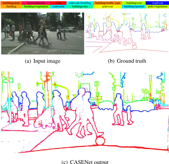
Figure 1. Edge detection and categorization with our approach. Given a street view image, our goal is to simultaneously detect the boundaries and assign each edge pixel with one or more semantic categories. (b) and (c) are color coded by HSV where hue and saturation together represent the composition and associated strengths of categories. Best viewed in color.

图 1: 采用我们方法实现的边缘检测与分类。给定街景图像，我们的目标是同时检测边界并为每个边缘像素分配一个或多个语义类别。(b) 和 (c) 采用 HSV 色彩编码，色相与饱和度共同表示类别组成及关联强度。建议彩色查看。

1. Introduction

1. 引言

Figure 1 shows an image of a road scene from Cityscapes dataset [8] with several object categories such as building, ground, sky, and car. In particular, we study the problem of simultaneously detecting edge pixels and classifying them based on association to one or more of the object categories [18, 42]. For example, an edge pixel lying on the contour separating building and pole can be associated with both of these object categories. In Figure 1, we visualize the boundaries and list the colors of typical category combinations such as “building $^+$ pole” and “road $^+$ sidewalk”. In our problem, every edge pixel is denoted by a vector whose individual elements denote the strength of pixel’s association with different semantic classes. While most edge pixels will be associated with only two object categories, in the case of junctions [37] one may expect the edge pixel to be associated with three or even more. We therefore do not restrict the number of object categories a pixel can be associated with, and formulate our task as a multi-label learning problem. In this paper, we propose CASENet, a deep network able to detect category-aware semantic edges. Given $K$ defined semantic categories, the network essentially produces $K$ separate edge maps where each map indicates the edge probability of a certain category. An example of separately visualized edge maps on a test image is given in Figure 2.

图1展示了一张来自Cityscapes数据集[8]的道路场景图像，其中包含建筑物、地面、天空和汽车等多个物体类别。我们重点研究同时检测边缘像素并根据其与一个或多个物体类别的关联进行分类的问题[18,42]。例如，位于建筑物与电线杆分界轮廓上的边缘像素可同时关联这两个物体类别。在图1中，我们通过可视化边界并标注典型类别组合（如"建筑物$^+$电线杆"和"道路$^+$人行道"）的颜色来展示这一概念。本研究中，每个边缘像素用一个向量表示，其各元素代表该像素与不同语义类别的关联强度。虽然多数边缘像素仅关联两个物体类别，但在交叉点[37]处可能关联三个甚至更多类别。因此我们不对像素可关联的类别数量设限，将该任务构建为多标签学习问题。本文提出CASENet深度网络用于检测类别感知的语义边缘。给定$K$个预定义的语义类别，该网络会生成$K$个独立的边缘概率图，每个图对应特定类别的边缘概率。图2展示了测试图像上各边缘概率图的可视化示例。

The problem of edge detection has been shown to be useful for a number of computer vision tasks such as segmentation [1, 3, 4, 6, 52], object proposal [3], 3d shape recovery [27], and 3d reconstruction [44]. By getting a better understanding of the edge classes and using them as prior or constraints, it is reasonable to expect some improvement in these tasks. With a little extrapolation, it is not difficult to see that a near-perfect semantic edge, without any additional information, can solve semantic segmentation, depth estimation [21, 38], image-based localization [24], and object detection [13]. We believe that it is important to improve the accuracy of semantic edge detection to a certain level for moving towards a holistic scene interpretation.

边缘检测问题已被证明对许多计算机视觉任务非常有用，例如分割 [1, 3, 4, 6, 52]、目标提议 [3]、3D形状恢复 [27] 和 3D重建 [44]。通过更好地理解边缘类别并将其作为先验或约束条件，可以合理预期这些任务会有所改进。稍加推演不难发现，近乎完美的语义边缘（无需任何额外信息）就能解决语义分割、深度估计 [21, 38]、基于图像的定位 [24] 和目标检测 [13] 等问题。我们认为，将语义边缘检测的精度提升到一定水平，对于实现整体场景理解至关重要。

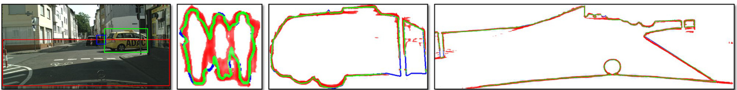
Figure 2. An example of a test image and zoomed edge maps corresponding to bounding box regions. The visualized edge maps belong to the categories of person, car and road, respectively. Green and blue denote correctly detected and missed edge pixels.

图 2: 测试图像示例及对应边界框区域的放大边缘图。可视化边缘图分别属于人物、汽车和道路类别。绿色和蓝色分别表示正确检测和漏检的边缘像素。

Early work tends to treat edge information as low-level cues to enhance other applications. However, the availability of large training data and the progress in deep learning methods have allowed one to make significant progress for the edge detection problem in the last few years. In particular, there have been newer data sets [18]. The availability of large-scale semantic segmentation data sets [8] can also be easily processed to obtain semantic edge data set as these two problems can be seen as dual problems.

早期研究倾向于将边缘信息视为增强其他应用的低层次线索。然而，随着大规模训练数据的可用性和深度学习方法的进步，近年来边缘检测问题取得了显著进展。特别是出现了更新的数据集[18]。大规模语义分割数据集[8]也可通过简单处理获得语义边缘数据集，因为这两个问题可视为对偶问题。

1.1. 相关工作

The definition of boundary or edge detection has evolved over time from low-level to high-level features: simple edge filters [5], depth edges [17], object boundaries [40], and semantic contours [18]. In some sense, the evolution of edge detection algorithms captures the progress in computer vision from simple convolutional filters such as Sobel [29] or Canny [5] to fully developed deep neural networks.

边界或边缘检测的定义随着时间从低级特征演进到高级特征：简单边缘滤波器 [5]、深度边缘 [17]、物体边界 [40] 和语义轮廓 [18]。从某种意义上说，边缘检测算法的演变体现了计算机视觉从 Sobel [29] 或 Canny [5] 等简单卷积滤波器到成熟的深度神经网络的进步。

Low-level edges Early edge detection methods used simple convolutional filters such as Sobel [29] or Canny [5].

低级边缘早期的边缘检测方法使用简单的卷积滤波器，如 Sobel [29] 或 Canny [5]。

Depth edges Some previous work focuses on labeling contours into convex, concave, and occluding ones from synthetic line drawings [38] and real world images under restricted settings [14, 17]. Indoor layout estimation can also be seen as the identification of concave boundaries (lines folding walls, ceilings, and ground) [20]. By recovering occluding boundaries [22], it was shown that the depth ordering of different layers in the scene can be obtained.

深度边缘
先前的一些工作专注于从合成线稿[38]和受限场景下的真实图像[14, 17]中将轮廓标记为凸面、凹面和遮挡边缘。室内布局估计也可视为对凹面边界(墙面、天花板与地面的折线)的识别[20]。通过恢复遮挡边界[22]，研究表明可以获取场景中不同层次的深度顺序。

Perceptual edges A wide variety of methods are driven towards the extraction of perceptual boundaries [40]. Dollar et al. [9] used boosted decision trees on different patches to extract edge maps. Lim et al. [33] computed sketch tokens which are object boundary patches using random forests. Several other edge detection methods include statistical edges [31], multi-scale boundary detection [43], and point-wise mutual information (PMI) detector [25]. More recently, Dollar and Zitnick [10] proposed a realtime fast edge detection method using structured random forests. Latest methods [3, 30, 50, 51] using deep neural networks have pushed the detection performance to state-of-the-art.

感知边缘
多种方法致力于提取感知边界 [40]。Dollar 等人 [9] 在不同图像块上使用提升决策树来提取边缘图。Lim 等人 [33] 通过随机森林计算了作为物体边界块的草图 token。其他几种边缘检测方法包括统计边缘 [31]、多尺度边界检测 [43] 以及点间互信息 (PMI) 检测器 [25]。最近，Dollar 和 Zitnick [10] 提出了一种使用结构化随机森林的实时快速边缘检测方法。采用深度神经网络的最新方法 [3, 30, 50, 51] 已将检测性能提升至最先进水平。

Semantic edges The origin of semantic edge detection can be possibly pinpointed to [42]. As a high level task, it has also been used implicitly or explicitly in many problems related to segmentation [49] and reconstruction [21]. In some sense, all semantic segmentation methods [7, 8, 12, 16, 35, 36, 41, 45, 48] can be loosely seen as semantic edge detection since one can easily obtain edges, although not necessarily an accurate one, from the segmentation results. There are papers that specifically formulate the problem statement as binary or category-aware semantic edge detection [3, 4, 13, 18, 28, 39, 42, 51]. Hariharan et al. [18] introduced the Semantic Boundaries Dataset (SBD) and proposed inverse detector which combines both bottom-up edge and top-down detector information to detect categoryaware semantic edges. HFL [3] first uses VGG [47] to locate binary semantic edges and then uses deep semantic segmentation networks such as FCN [36] and DeepLab [7] to obtain category labels. The framework, however, is not endto-end trainable due to the separated prediction process.

语义边缘
语义边缘检测的起源可以追溯到[42]。作为一项高级任务，它已隐式或显式地应用于许多与分割[49]和重建[21]相关的问题中。从某种意义上说，所有语义分割方法[7,8,12,16,35,36,41,45,48]都可以粗略地视为语义边缘检测，因为从分割结果中可以轻松获得边缘（尽管不一定是精确的）。有些论文专门将问题表述为二值或类别感知的语义边缘检测[3,4,13,18,28,39,42,51]。Hariharan等人[18]引入了语义边界数据集(SBD)，并提出了一种结合自底向上边缘和自顶向下检测器信息的逆向检测器来检测类别感知的语义边缘。HFL[3]首先使用VGG[47]定位二值语义边缘，然后使用FCN[36]和DeepLab[7]等深度语义分割网络获取类别标签。然而，由于预测过程分离，该框架无法端到端训练。

DNNs for edge detection Deep neural networks recently became popular for edge detection. Related work includes SCT based on sparse coding [37], $N^{4}$ fields [15], deep contour [46], deep edge [2], and CSCNN [23]. One notable method is the holistic ally-nested edge detection (HED) [50] which trains and predicts edges in an image-to-image fashion and performs end-to-end training.

用于边缘检测的DNN
深度神经网络最近在边缘检测领域变得流行。相关研究包括基于稀疏编码的SCT [37]、$N^{4}$ fields [15]、deep contour [46]、deep edge [2]以及CSCNN [23]。其中值得注意的方法是整体嵌套边缘检测(HED) [50]，它以图像到图像的方式进行训练和预测，并执行端到端训练。

1.2. Contributions

1.2. 贡献

Our work is related to HED in adopting a nested architecture but we extend the work to the more difficult categoryaware semantic edge detection problem. Our main contributions in this paper are summarized below:

我们的工作与HED在采用嵌套架构方面相关，但我们将研究扩展到了更具挑战性的类别感知语义边缘检测问题。本文的主要贡献总结如下：

• To address edge categorization, we propose a multilabel learning framework which allows improved edge learning than traditional multi-class framework. • We propose a novel nested architecture without deep supervision on ResNet [19], where bottom features are only used to augment top classifications. We show that deep supervision may not be beneficial in our problem. • We outperform previous state-of-the-art methods by significant margins on SBD and Cityscapes datasets.

• 为解决边缘分类问题，我们提出了一种多标签学习框架，相比传统多类框架能实现更优的边缘学习效果。
• 我们在ResNet[19]基础上提出了一种无需深度监督的新型嵌套架构，底层特征仅用于增强顶层分类。实验表明深度监督对本研究问题并无助益。
• 在SBD和Cityscapes数据集上，我们的方法以显著优势超越了现有最优方法。

2. Problem Formulation

2. 问题表述

Given an input image, our goal is to compute the semantic edge maps corresponding to pre-defined categories. More formally, for an input image $\mathbf{I}$ and $K$ defined semantic categories, we are interested in obtaining $K$ edge maps ${\mathbf{Y}{1},\cdots,\mathbf{Y}{K}}$ , each having the same size as I. With a network having the parameters $\mathbf{W}$ , we denote $\mathbf{Y}_{k}(\mathbf{p}|\mathbf{I},$ $\mathbf{W})\in[0,1]$ as the network output indicating the computed edge probability on the $k$ -th semantic category at pixel $\mathbf{p}$ .

给定输入图像，我们的目标是计算与预定义类别对应的语义边缘图。更正式地说，对于输入图像 $\mathbf{I}$ 和 $K$ 个定义的语义类别，我们希望获得 $K$ 个边缘图 ${\mathbf{Y}{1},\cdots,\mathbf{Y}{K}}$，每个边缘图与 I 尺寸相同。对于参数为 $\mathbf{W}$ 的网络，我们将 $\mathbf{Y}_{k}(\mathbf{p}|\mathbf{I},$ $\mathbf{W})\in[0,1]$ 表示为网络输出，指示像素 $\mathbf{p}$ 处第 $k$ 个语义类别的计算边缘概率。

2.1. Multi-label loss function

2.1. 多标签损失函数

Possibly driven by the multi-class nature of semantic segmentation, several related works on category-aware semantic edge detection have more or less looked into the problem from the multi-class learning perspective. Our intuition is that this problem by nature should allow one pixel belonging to multiple categories simultaneously, and should be addressed by a multi-label learning framework.

可能受到语义分割多类别特性的驱动，一些关于类别感知语义边缘检测的相关工作或多或少从多类别学习的角度探讨了这一问题。我们的直觉是，该问题本质上应允许一个像素同时属于多个类别，并应通过多标签学习框架来解决。

We therefore propose a multi-label loss. Suppose each image I has a set of label images ${\bar{\bf Y}{1},\cdot\cdot\cdot,\bar{\bf Y}{K}}$ , where $\bar{\mathbf{Y}}{k}$ is a binary image indicating the ground truth of the $k$ -th class semantic edge.

因此我们提出一种多标签损失函数。假设每幅图像I有一组标签图像${\bar{\bf Y}{1},\cdot\cdot\cdot,\bar{\bf Y}{K}}$，其中$\bar{\mathbf{Y}}_{k}$是表示第$k$类语义边缘真实值的二值图像。

where $\beta$ is the percentage of non-edge pixels in the image to account for skewness of sample numbers, similar to [50].

其中 $\beta$ 是图像中非边缘像素的百分比，用于平衡样本数量的偏斜，类似于 [50]。

3. Network Architecture

3. 网络架构

We propose CASENet, an end-to-end trainable convolutional neural network (CNN) architecture (shown in Fig. 3(c)) to address category-aware semantic edge detection. Before describing CASENet, we first propose two alternative network architectures which one may come up with straightforwardly given the abundant previous literature on edge detection and semantic segmentation. Although both architectures can also address our task, we will analyze issues associated with them, and address these issues by proposing the CASENet architecture.

我们提出CASENet，一种端到端可训练的卷积神经网络(CNN)架构(如图3(c)所示)，用于解决类别感知语义边缘检测问题。在描述CASENet之前，我们首先提出两种替代网络架构，这两种架构是基于边缘检测和语义分割领域大量现有文献可以直接想到的。虽然这两种架构也能解决我们的任务，但我们将分析它们存在的问题，并通过提出CASENet架构来解决这些问题。

3.1. Base network

3.1. 基础网络

We address the edge detection problem under the fully convolutional network framework. We adopt ResNet-101 by removing the original average pooling and fully connected layer, and keep the bottom convolution blocks. We further modify the base network in order to better preserve low-level edge information. We change the stride of the first and fifth convolution blocks (“res1” and “res5” in Fig. 3) in ResNet-101 from 2 to 1. We also introduce dilation factors to subsequent convolution layers to maintain the same receptive field sizes as the original ResNet, similar to [19].

我们在全卷积网络框架下解决边缘检测问题。采用ResNet-101架构时移除了原始的平均池化层和全连接层，仅保留底部卷积块。为进一步优化低级边缘信息保留效果，我们对基础网络进行了改进：将ResNet-101中第一和第五卷积块（图3中的"res1"和"res5"）的步长从2调整为1，并参照[19]的方法在后续卷积层引入膨胀系数，以保持与原始ResNet相同的感受野大小。

3.2. Basic architecture

3.2. 基础架构

A very natural architecture one may come up with is the Basic architecture shown in Fig. 3(a). On top of the base network, we add a classification module (Fig. 3(d)) as a $1\times1$ convolution layer, followed by bilinear up-sampling (implemented by a $K$ -grouped de convolution layer) to produce a set of $K$ activation maps ${\mathbf{A}{1},\cdots,\mathbf{A}{K}}$ , each having the same size as the image. We then model the probability of a pixel belonging to the $k$ -th class edge using the sigmoid unit given by $\mathbf{Y}{k}(\mathbf{p}):=:\sigma(\mathbf{A}{k}(\mathbf{p}))$ , which is presented in the Eq. (1). Note that $\mathbf{Y}_{k}(\mathbf{p})$ is not mutually exclusive.

一个非常自然的架构可能是图3(a)所示的基础架构。在基础网络之上，我们添加了一个分类模块（图3(d)），作为1×1卷积层，随后通过双线性上采样（由K组分组的反卷积层实现）生成一组K个激活图{𝐀₁,⋯,𝐀ₖ}，每个图的大小与图像相同。然后，我们使用sigmoid单元对像素属于第k类边缘的概率进行建模，由𝐘ₖ(𝐩) = σ(𝐀ₖ(𝐩))给出，如式(1)所示。需要注意的是，𝐘ₖ(𝐩)并不是互斥的。

3.3. Deeply supervised architecture

3.3. 深度监督架构

One of the distinguishing features of the holistic allynested edge detection (HED) network [50] is the nested architecture with deep supervision [32]. The basic idea is to impose losses to bottom convolution sides besides the top network loss. In addition, a fused edge map is obtained by supervising the linear combination of side activation s.

整体嵌套边缘检测 (HED) 网络 [50] 的显著特征之一是其采用深度监督 [32] 的嵌套架构。核心思想是在顶层网络损失之外，对底层卷积侧输出施加损失约束。此外，通过监督各侧输出激活的线性组合，最终融合得到边缘检测图。

Note that HED only performs binary edge detection. We extended this architecture to handle $K$ channels for side outputs and $K$ channels for the final output. We refer to this as deeply supervised network (DSN), as depicted in Fig. 3(b). In this network, we connect an above-mentioned classification module to the output of each stack of residual blocks, producing 5 side classification activation maps ${\mathbf{A}^{(1)},\ldots,\mathbf{\bar{A}}^{(5)}}$ , where each of them has $K$ -channels. We then fuse these 5 activation maps through a sliced concatenation layer (the color denotes the channel index in Fig. $3(\mathrm{g}),$ ) to produce a $5K$ -channel activation map:

需要注意的是，HED仅执行二值边缘检测。我们扩展了这一架构，使其能够处理侧边输出的$K$个通道和最终输出的$K$个通道。我们将此称为深度监督网络(DSN)，如图3(b)所示。在该网络中，我们将上述分类模块连接到每组残差块的输出端，生成5个侧边分类激活图${\mathbf{A}^{(1)},\ldots,\mathbf{\bar{A}}^{(5)}}$，每个激活图均具有$K$个通道。随后通过切片拼接层(图$3(\mathrm{g})$中颜色表示通道索引)融合这5个激活图，生成一个$5K$通道的激活图：

$$
\mathbf{A}^{f}={\mathbf{A}{1}^{(1)},\ldots,\mathbf{A}{1}^{(5)},\mathbf{A}{2}^{(1)},\ldots,\mathbf{A}{2}^{(5)},\ldots,\mathbf{A}_{K}^{(5)}}
$$

$\mathbf{A}^{f}$ is fed into our fused classification layer which performs $K$ -grouped $1\times1$ convolution (Fig. 3(f)) to produce a $K$ - channel activation map $\mathbf{A}^{(6)}$ . Finally, 6 loss functions are computed on ${\mathbf{A}^{(1)},\ldots,\mathbf{A}^{(6)}}$ using the Equation 1 to provide deep supervision to this network.

$\mathbf{A}^{f}$ 被输入到我们的融合分类层中，该层执行 $K$ 组分组的 $1\times1$ 卷积（图 3(f)）以生成一个 $K$ 通道的激活图 $\mathbf{A}^{(6)}$。最后，使用公式 1 在 ${\mathbf{A}^{(1)},\ldots,\mathbf{A}^{(6)}}$ 上计算 6 个损失函数，以对该网络进行深度监督。

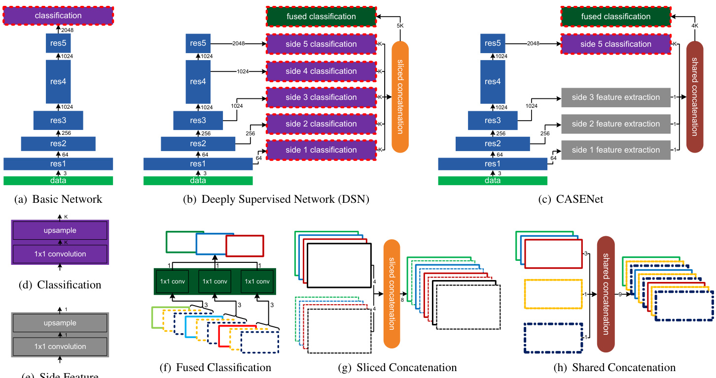
Figure 3. Three CNN architectures designed in this paper are shown in (a)-(c). A solid rectangle represents a composite block of CNN layers. Any decrease of its width indicates a drop of spatial resolution of this block’s output feature map by a factor of 2. A number besides an arrow indicates the number of channels of the block’s output features. A blue solid rectangle is a stack of ResNet blocks. A purple solid rectangle is our classification module. A dotted red outline indicates that block’s output is supervised by our loss function in equation 1. A gray solid rectangle is our side feature extraction module. A dark green solid rectangle is our fused classification module performing $K$ -grouped $1\times1$ convolution. (d)-(h) depicts more details of various modules used in (a)-(c), where outlined rectangles illustrate input and output feature maps. Best viewed in color.

图 3: (a)-(c)展示了本文设计的三种CNN架构。实线矩形代表CNN层的复合模块，宽度缩减表示该模块输出特征图的空间分辨率降低为原来的1/2。箭头旁的数字表示模块输出特征的通道数。蓝色实线矩形为ResNet模块堆叠，紫色实线矩形为分类模块，红色虚线框表示该模块输出受公式1的损失函数监督，灰色实线矩形为侧边特征提取模块，深绿色实线矩形为执行$K$组$1\times1$卷积的融合分类模块。(d)-(h)详细展示了(a)-(c)中各模块结构，其中框线矩形表示输入输出特征图。建议彩色查看。

Note that the reason we perform sliced concatenation in conjunction with grouped convolution instead of the corresponding conventional operations is as follows. Since the 5 side activation s are supervised, we implicitly constrain each channel of those side activation s to carry information that is most relevant to the corresponding class.

需要注意的是，我们之所以采用切片级联 (sliced concatenation) 与分组卷积 (grouped convolution) 结合的方式，而非传统对应操作，原因如下：由于5个侧输出激活受到监督，我们隐式约束了这些侧输出激活的每个通道，使其携带与对应类别最相关的信息。

With sliced concatenation and grouped convolution, the fused activation for a pixel $\mathbf{p}$ is given by:

采用切片拼接和分组卷积后，像素 $\mathbf{p}$ 的融合激活计算方式为：

$$
{\bf A}{k}^{(6)}({\bf p})=W_{k}^{T}[{\bf A}{k}^{(1)}({\bf p})^{T},\cdot\cdot\cdot,{\bf A}_{k}^{(5)}({\bf p})^{T}]
$$

This essentially integrates corresponding class-specific activations from different scales as the finally fused activation s. Our experiments empirically support this design choice.

这本质上将不同尺度下对应的类别特定激活整合为最终融合的激活s。我们的实验从经验上支持这一设计选择。

3.4. CASENet architecture

3.4. CASENet架构

Upon reviewing the Basic and DSN architectures, we notice several potential associated issues in the category-aware semantic edge detection task:

在审视基础架构和DSN架构后，我们注意到类别感知语义边缘检测任务中存在几个潜在关联问题：

First, the receptive field of the bottom side is limited. As a result it may be unreasonable to require the network to perform semantic classification at an early stage, given that context information plays an important role in semantic classification. We believe that semantic classification should rather happen on top where features are encoded with high-level information.

首先，底部的感受野有限。因此，考虑到上下文信息在语义分类中的重要作用，要求网络在早期阶段进行语义分类可能并不合理。我们认为，语义分类更应该发生在高层信息编码的特征顶部。

Second, bottom side features are helpful in augmenting top classifications, suppressing non-edge pixels and providing detailed edge localization and structure information. Hence, they should be taken into account in edge detection.

其次，底部特征有助于增强顶部分类，抑制非边缘像素，并提供精确的边缘定位和结构信息。因此，在边缘检测中应予以考虑。

Our proposed CASENet architecture (Fig. 3(c)) is motivated by addressing the above issues. The network adopts a nested architecture which to some extent shares similarity to DSN but also contains several key improvements. We summarize these improvements below:

我们提出的CASENet架构(图3(c))旨在解决上述问题。该网络采用嵌套架构，在某种程度上与DSN有相似之处，但包含了几项关键改进。我们将这些改进总结如下:

The difference between side feature extraction and side classification is that the former only outputs a single channel feature map $\mathbf{F}^{\left(j\right)}$ rather than $K$ class activation s. The shared concatenation replicates the bottom features $\mathbf{F} =~{\mathbf{F}^{(1)}$ , ${\bf F}^{(2)},{\bf F}^{(3)}}$ from Side-1-3 to separately concatenate with each of the $K$ top activation s:

侧边特征提取与侧边分类的区别在于，前者仅输出单通道特征图 $\mathbf{F}^{\left(j\right)}$ 而非 $K$ 个类别激活图。共享拼接操作会将底层特征 $\mathbf{F} =~{\mathbf{F}^{(1)}$ , ${\bf F}^{(2)},{\bf F}^{(3)}}$ 从Side-1-3复制出来，分别与 $K$ 个顶层激活图进行拼接：

$$
\mathbf{A}^{f}={\mathbf{F},\mathbf{A}{1}^{(5)},\mathbf{F},\mathbf{A}{2}^{(5)},\mathbf{F},\mathbf{A}{3}^{(5)},\dots,\mathbf{F},\mathbf{A}_{K}^{(5)}}.
$$

The resulting concatenated activation map is again fed into the fused classification layer with $K$ -grouped convolution to produce a $K$ -channel activation map $\mathbf{A}^{(\bar{6})}$ .

生成的拼接激活图再次输入到融合分类层中，通过 $K$ 分组卷积生成一个 $K$ 通道的激活图 $\mathbf{A}^{(\bar{6})}$。

In general, CASENet can be thought of as a joint edge detection and classification network by letting lower level features participating and augmenting higher level semantic classification through a skip-layer architecture.

一般而言，CASENet可被视为通过跳跃连接架构让低层特征参与并增强高层语义分类的边缘检测与分类联合网络。

4. Experiments

4. 实验

In this paper, we compare CASENet1 with previous state-of-the-art methods, including InvDet [18], HFL [3], weakly supervised object boundaries [28], as well as several baseline network architectures.

在本文中，我们将CASENet1与之前的最先进方法进行比较，包括InvDet [18]、HFL [3]、弱监督物体边界 [28]以及几种基线网络架构。

4.1. Datasets

4.1. 数据集

We evaluate the methods on SBD [18], a standard dataset for benchmarking semantic edge detection. Besides SBD, we also extend our evaluation to Cityscapes [8], a popular semantic segmentation dataset with pixel-level high quality annotations and challenging street view scenarios. To the best of our knowledge, our paper is the first work to formally report semantic edge detection results on this dataset.

我们在SBD [18]（语义边缘检测基准测试的标准数据集）上评估了这些方法。除SBD外，我们还将评估扩展到Cityscapes [8]——一个具有像素级高质量标注和具有挑战性街景场景的流行语义分割数据集。据我们所知，本文是首个在该数据集上正式报告语义边缘检测结果的工作。

SBD The dataset consists of 11355 images from the PASCAL VOC2011 [11] trainval set, divided into 8498 training and 2857 test images2. This dataset has semantic boundaries labeled with one of 20 Pascal VOC classes.

SBD数据集包含来自PASCAL VOC2011 [11]训练验证集的11355张图像，划分为8498张训练图像和2857张测试图像。该数据集标注了20个Pascal VOC类别的语义边界。

Cityscapes The dataset contains 5000 images divided into 2975 training, 500 validation and 1525 test images. Since the labels of test images are currently not available, we treat the validation images as test set in our experiment.

Cityscapes数据集包含5000张图像，分为2975张训练集、500张验证集和1525张测试集。由于测试集标签暂未公开，实验中我们将验证集视为测试集使用。

4.2. Evaluation protocol

4.2. 评估协议

On both SBD and Cityscapes, the edge detection accuracy for each class is evaluated using the official benchmark code and ground truth from [18]. We keep all settings and parameters as default, and report the maximum F-measure (MF) at optimal dataset scale (ODS), and average precision (AP) for each class. Note that for Citiscapes, we follow [18] exactly to generate ground truth boundaries with single pixel width for evaluation, and reduce the sizes of both ground truth and predicted edge maps to half along each dimension considering the speed of evaluation.

在SBD和Cityscapes数据集上，我们使用[18]提供的官方基准代码和真实标注（ground truth）评估每个类别的边缘检测准确率。所有设置和参数均保持默认，报告最优数据集尺度（ODS）下的最大F值（MF）以及每个类别的平均精度（AP）。需要注意的是，对于Cityscapes数据集，我们严格遵循[18]的方法生成单像素宽度的真实边界用于评估，并将真实标注和预测边缘图的尺寸沿每个维度缩小一半以提升评估速度。

4.3. Implementation details

4.3. 实现细节

We trained and tested CASENet, HED [50], and the proposed baseline architectures using the Caffe library [26].

我们使用Caffe库[26]对CASENet、HED[50]以及提出的基线架构进行了训练和测试。

Training labels Considering the misalignment between human annotations and true edges, and the label ambiguity of pixels near boundaries, we generate slightly thicker ground truth edges for network training. This can be done by looking into neighbors of a pixel and seeking any difference in segmentation labels. The pixel is regarded as an edge pixel if such difference exists. In our paper, we set the maximum range of neighborhood to be 2. Under the multilabel framework, edges from different classes may overlap.

训练标签
考虑到人工标注与真实边缘之间的不对齐，以及边界附近像素的标签模糊性，我们为网络训练生成了稍厚的真实边缘。这可以通过查看像素的邻域并寻找分割标签中的差异来实现。如果存在这种差异，则该像素被视为边缘像素。在我们的论文中，将邻域的最大范围设置为2。在多标签框架下，来自不同类别的边缘可能会重叠。

Baselines Since several main comparing methods such as HFL and HED use VGG or VGG based architectures for edge detection and categorization, we also adopt the CASENet and other baseline architectures on VGG (denoted as CASENet-VGG). In particular, we remove the max pooling layers after conv4, and keep the resolutions of conv5, fc6 and fc7 the same as conv4 (1/8 of input). Similar to [7], both fc6 and fc7 are treated as convolution layers with $3\times3$ and $1\times1$ convolution and dimensions set to 1024. Dilation factors of 2 and 4 are applied to conv5 and fc6.

基线方法
由于HFL、HED等主要对比方法均采用VGG或基于VGG的架构进行边缘检测与分类，我们同样在VGG上采用CASENet及其他基线架构（记为CASENet-VGG）。具体而言，我们移除了conv4后的最大池化层，并保持conv5、fc6和fc7的分辨率与conv4一致（输入尺寸的1/8）。参照[7]，fc6和fc7均被视为卷积层，分别采用$3\times3$和$1\times1$卷积核，维度设为1024。conv5和fc6分别设置膨胀因子为2和4。

To compare our multi-label framework with multi-class, we generate ground truth with non-overlapping edges of each class, reweight the softmax loss similar to our paper, and replace the top with a 21-class reweighted softmax loss.

为了比较我们的多标签框架与多分类方法，我们生成每个类别非重叠边缘的真实标签，采用与论文类似的softmax损失重加权方式，并将顶层替换为21类重加权softmax损失。

Initialization In our experiment, we initialize the convolution blocks of ResNet/VGG in CASENet and all comparing baselines with models pre-trained on MS COCO [34].

初始化
在我们的实验中，我们使用在 MS COCO [34] 上预训练的模型来初始化 CASENet 及所有对比基线中 ResNet/VGG 的卷积块。

Hyper-parameters We unify the hyper-parameters for all comparing methods with the same base network, and set most of them following HED. In particular, we perform SGD with iteration size of 10, and fix loss weight to be 1, momentum 0.9, and weight decay 0.0005. For methods with ResNet, we set the learning rate, step size, gamma and crop size to $1e\mathrm{-~}7/5e\mathrm{ -~}8.$ , 10000 / 20000, $0.1/0.2$ and $352\times352/472\times472$ respectively for SBD and Cityscapes. For VGG, the learning rate is set to $1e-8$ while others remain the same as ResNet on SBD. For baselines with softmax loss, the learning rate is set to 0.01 while other parameters remain the same. The iteration numbers on SBD and Cityscapes are empirically set to 22000 and 40000.

超参数
我们统一了所有基于相同基础网络的对比方法的超参数，并参照HED设置了大部分参数。具体而言，我们采用迭代次数为10的SGD优化器，固定损失权重为1，动量(momentum)为0.9，权重衰减(weight decay)为0.0005。对于使用ResNet的方法，在SBD和Cityscapes数据集上分别设置学习率为$1e\mathrm{ -~}7/5e\mathrm{ -~}8$，步长(step size)为10000/20000，$\gamma$为$0.1/0.2$，裁剪尺寸(crop size)为$352\times352/472\times472$。对于VGG网络，在SBD数据集上学习率设为$1e-8$，其余参数与ResNet保持一致。采用softmax损失的基线方法学习率设为0.01，其他参数保持不变。SBD和Cityscapes的迭代次数根据经验分别设置为22000和40000。

Data augmentation During training, we enable random mirroring and cropping on both SBD and Cityscapes. We additionally augment the SBD data by resizing each image with scaling factors ${0.5,0.75,1.0,1.25,1.5}$ , while no such augmentation is performed on Cityscapes.

数据增强
在训练过程中，我们对SBD和Cityscapes数据集启用了随机镜像和裁剪。此外，我们通过以缩放因子 ${0.5,0.75,1.0,1.25,1.5}$ 调整每张图像的大小来增强SBD数据，而Cityscapes未进行此类增强。

4.4. Results on SBD

4.4. SBD 实验结果

Table 1 shows the MF scores of different methods performing category-wise edge detection on SBD, where CASENet outperforms previous methods. Upon using the benchmark code from [18], one thing we notice is that the recall scores of the curves are not monotonically increasing, mainly due to the fact that post-processing is taken after threshold ing in measuring the precision and recall rates. This is reasonable since we have not taken any post processing operations on the obtained raw edge maps. We only report the MF on SBD since AP is not well defined under such situation. The readers may kindly refer to supplementary materials for class-wise precision recall curves.

表 1 展示了不同方法在 SBD 数据集上进行类别感知边缘检测的 MF (Matched F-score) 分数，其中 CASENet 的表现优于先前的方法。在使用 [18] 提供的基准代码时，我们注意到召回率曲线并非单调递增，这主要是由于在计算精确率和召回率时，阈值处理之后还进行了后处理。这一现象是合理的，因为我们未对获取的原始边缘图进行任何后处理操作。由于在此情况下 AP (Average Precision) 的定义不够明确，我们仅报告了 SBD 上的 MF 分数。读者可参考补充材料查看各类别的精确率-召回率曲线。

Multi-label or multi-class? We compare the proposed multi-label loss with the reweighted softmax loss under the Basic architecture. One could see that using softmax leads to significant performance degradation on both VGG and ResNet, supporting our motivation in formulating the task as a multi-label learning problem, in contrast to the well accepted concept which addresses it in a multi-class way.

多标签还是多类别？我们比较了基础架构下提出的多标签损失与重新加权的softmax损失。可以看出，使用softmax会导致VGG和ResNet性能显著下降，这支持了我们将该任务表述为多标签学习问题的动机，而非广泛接受的将其视为多类别问题的方式。

Is deep supervision necessary? We compare CASENet with baselines network architectures including Basic and DSN depicted in Fig. 3. The result empirically supports our intuition that deep supervision on bottom sides may not be necessary. In particular, CASENet wins frequently on per-class MF as well as the final mean MF score. Our observation is that the annotation quality to some extent influenced the network learning behavior and evaluation, leading to less performance distinctions across different methods. Such distinction becomes more obvious on Cityscapes.

深度监督是否必要？我们将CASENet与图3所示的Basic和DSN等基线网络架构进行比较。结果从经验上支持了我们的直觉：底层的深度监督可能并非必要。特别是，CASENet在每类MF以及最终平均MF分数上频繁胜出。我们观察到，标注质量在一定程度上影响了网络学习行为和评估，导致不同方法间的性能差异较小。这种差异在Cityscapes数据集上更为明显。

Is top supervision necessary? One might further question the necessity of imposing supervision on Side-5 activa- tion in CASENet. We use CASENet− to denote the same CASENet architecture without Side-5 supervision during training. The improvement upon adding Side-5 supervision indicates that a supervision on higher level side activation is helpful. Our intuition is that Side-5 supervision helps Side5 focusing more on the classification of semantic classes with less influence from interacting with bottom layers.

是否需要顶部监督？有人可能会进一步质疑在CASENet中对Side-5激活施加监督的必要性。我们使用CASENet−表示训练期间没有Side-5监督的相同CASENet架构。添加Side-5监督后的改进表明，对更高层侧激活的监督是有帮助的。我们的直觉是，Side-5监督有助于Side5更专注于语义类别的分类，减少与底层交互的影响。

Visualizing side activation s We visualize the results of CASENet, CASENet− and DSN on a test image in Fig. 5. Overall, CASENet achieves better detection compared to the other two. We further show the side activation s of this testing example in Fig. 6, from which one can see that the activation s of DSN on Side-1, Side-2 and Side-3 are more blurry than CASENet features. This may be caused by imposing classification requirements on those layers, which seems a bit aggressive given limited receptive field and information and may caused performance degradation. Also one may notice the differences in “Side5-Person” and “Side5-Boat” between CASENet− and CASENet, where CASENet’s activation s overall contain sharper edges, again showing the benefit of Side-5 supervision.

可视化侧边激活
我们在图5中展示了CASENet、CASENet−和DSN在一张测试图像上的结果。总体而言，CASENet相比其他两种方法实现了更好的检测效果。我们在图6中进一步展示了该测试样本的侧边激活情况，可以看出DSN在Side-1、Side-2和Side-3上的激活比CASENet的特征更加模糊。这可能是由于对这些层施加了分类要求，考虑到有限的感受野和信息量，这种做法显得较为激进，可能导致性能下降。此外，可以观察到CASENet−和CASENet在"Side5-Person"和"Side5-Boat"上的差异，其中CASENet的激活整体包含更清晰的边缘，再次证明了Side-5监督的优势。

Figure 4. Training losses of different variants of CASENet on the SBD dataset. The losses are respectively moving averaged by a kernel length of 8000. All curves means the final fused losses, except for CASENet-side5 which indicates the loss of Side-5’s output. Note that CASENet loss is consistently the smallest.

图 4: 不同CASENet变体在SBD数据集上的训练损失。所有损失均采用8000长度的滑动窗口进行平滑处理。除标注为Side-5输出的CASENet-side5曲线外，其余曲线均表示最终融合损失。值得注意的是，CASENet的损失始终最小。

From ResNet to VGG CASENet-VGG in Table 1 shows comparable performance to HFL-FC8. HFL-CRF performs slightly better with the help of CRF post processing. The results to some extent shows the effectiveness our learning framework, given HFL uses two VGG networks separately for edge localization and classification. Our method also significantly outperforms the HED baselines from [28], which gives 44 / 41 on MF / AP, and $49/45$ with detection.

表1中的CASENet-VGG显示其性能与HFL-FC8相当。借助CRF后处理，HFL-CRF表现略优。这些结果在一定程度上证明了我们学习框架的有效性，因为HFL使用了两个独立的VGG网络分别进行边缘定位和分类。我们的方法也显著优于[28]中的HED基线（MF/AP为44/41，检测时为$49/45$）。

Other variants We also investigated several other architectures. For example, we kept the stride of 2 in “res1”. This downgrades the performance for lower input resolution. Another variant is to use the same CASENet architec- ture but impose binary edge losses (where a pixel is considered lying on an edge as long as it belongs to the edge of at least one class) on Side-1-3 (denoted as CASENet-edge in Fig. 4). However we found that such supervision seems to be a divergence to the semantic classification at Side-5.

其他变体
我们还研究了其他几种架构。例如，在"res1"中保持步长为2，这会降低较低输入分辨率下的性能。另一种变体是使用相同的CASENet架构，但在Side-1-3上施加二值边缘损失（只要像素属于至少一个类别的边缘，即被视为位于边缘上）(在图4中标记为CASENet-edge)。然而我们发现，这种监督方式似乎与Side-5的语义分类存在分歧。

4.5. Results on Cityscapes

4.5. Cityscapes 数据集上的结果

We also train and test both DSN and CASENet with ResNet as base network on the Cityscapes. Compared to SBD, Cityscapes has relatively higher annotation quality but contains more challenging scenarios. The dataset contains more overlapping objects, which leads to more cases of multi-label semantic boundary pixels and thus may be better to test the proposed method. In Table 1, we provide both MF and AP of the comparing methods. To the best of our knowledge, this is the first paper quantitatively reporting the detection performance of category-wise semantic edges on Cityscapes. One could see CASENet consistently outperforms DSN in all classes with a significant margin. Besides quantitative results, we also visualize some results in Fig. 7 for qualitative comparisons.

我们还在Cityscapes数据集上以ResNet为基干网络对DSN和CASENet进行了训练和测试。与SBD相比，Cityscapes的标注质量相对更高，但包含更具挑战性的场景。该数据集含有更多重叠物体，导致多标签语义边界像素的情况更普遍，因此可能更适合测试所提出的方法。在表1中，我们列出了对比方法的MF (mean F-score) 和AP (average precision)。据我们所知，这是首篇定量报告Cityscapes数据集中类别语义边缘检测性能的论文。可以看到，CASENet在所有类别上都显著优于DSN。除定量结果外，我们还在图7中可视化了一些结果用于定性比较。

able 1. Results on the SBD benchmark. All MF scores are measured by $%$ .

表 1: SBD 基准测试结果。所有 MF 分数均以 $%$ 为单位测量。

| 指标 | 类别 | 方法 | aero | bike | bird | boat | bottle | bus | car | cat | chair | cOW | table | dog | horse | mbike | person | plant | sheep | sofa | train | tv |
|------|------|------|------|------|------|------|--------|-----|-----|-----|-------|-----|-------|-----|-------|-------|--------|-------|-------|------|------|
| | InvDet Baseline | | 41.5 | 46.7 | 15.6 | 17.1 54.1 | 36.5 | 42.6 | 40.3 | 22.7 | 18.9 | 26.9 | 12.5 | 18.2 | 35.4 67.5 | 29.4 62.2 | 48.2 | 13.9 | 26.9 | 11.1 | 21.9 | 31.4 | 27.9 58.7 |
| | HFL-FC8 | | 71.6 | 59.6 | 68.0 | | 57.2 | 68.0 | 58.8 | 69.3 | 43.3 | 65.8 | 33.3 | 67.9 | | | | 69.0 | 43.8 | 68.5 | 33.9 | 57.7 | 54.8 |
| | HFL-CRF | | 73.9 | 61.4 | 74.6 | 57.2 | 58.8 | 70.4 | 61.6 | 71.9 | 46.5 | 72.3 | 36.2 | 71.1 | 73.0 | 68.1 | 70.3 | 44.4 | 73.2 | 42.6 | | 62.4 | 62.5 |
| | Basic-Softmax | | 67.6 | 55.3 | 50.4 | | 42.3 | 64.6 | 61.0 | 63.9 | 37.4 | 43.1 | 25.3 | 57.9 | 57.1 | 60.0 | 72.0 | 33.0 | 53.5 | 30.9 | 54.4 | 47.7 | 51.1 |
| | VGG Basic | | 70.0 | 58.6 | 62.5 | | 51.2 | 65.4 | 60.6 | 66.9 | 39.7 | 47.3 | 31.0 | 60.1 | 59.4 | 60.2 | 74.4 | 38.0 | 56.0 | 35.9 | 60.0 | 53.8 | 55.1 |
| | CASENet | | 72.5 | 61.5 | 63.8 | | 52.3 | 65.4 | 62.6 | 67.2 | 42.6 | 51.8 | 31.4 | 62.0 | 61.9 | 62.8 | 75.4 | 41.7 | 59.8 | 35.8 | 59.7 | 50.7 | 56.8 |
| | Basic-Softmax | | 74.0 | 64.1 | 64.8 | | 52.1 | 73.2 | 68.1 | 73.2 | 43.1 | 56.2 | 37.3 | 67.4 | 68.4 | 67.6 | 76.7 | 42.7 | 64.3 | 37.5 | 64.6 | 56.3 | 60.2 |
| | Basic | | 82.5 | 74.2 | 80.2 | | 68.0 | 80.8 | 74.3 | 82.9 | 52.9 | 73.1 | 46.1 | 79.6 | 78.9 | 76.0 | 80.4 | 52.4 | 75.4 | 48.6 | 75.8 | 68.0 | 70.6 |
| | ResNet DSN | | 81.6 | 75.6 | 78.4 | 61.3 | 67.6 | 82.3 | 74.6 | 82.6 | 52.4 | 71.9 | 45.9 | 79.2 | 78.3 80.4 | 76.2 76.2 | 80.1 80.2 | 51.9 53.2 | 74.9 | 48.0 47.7 | 76.5 75.6 | 66.8 66.3 | 70.3 |
| | CASENet" | 83.0 83.3 | 74.7 76.0 | 79.6 80.7 | 61.5 63.4 | 67.7 | 80.7 81.3 | 74.1 74.9 | 82.8 83.2 | 53.3 54.3 | 75.0 | 44.5 46.4 | 79.8 | | 76.6 | | | | 77.3 | | | | 70.7 71.4 |
| | CASENet | | | | | 69.2 | | | | | 74.8 | | 80.3 | 80.2 | | | | 53.3 | 77.2 | 50.1 | 75.9 | 8'99 | |

Table 2. Results on the Cityscapes dataset. All MF and AP scores are measured by $%$ .

指标	方法	道路	人行道	建筑	墙面	围栏		杆子	交通灯	交通标志	植被	地形	天空	行人	骑行者	汽车	卡车		巴士	火车	摩托车		自行车	平均值
MF	DSN	85.4	76.4	82.6	51.8		56.5	66.5	62.6	72.1	80.6	61.1	76.0		77.5	66.3	84.5	52.3	67.3		49.4	56.0	76.0	68.5
	CASENet	86.6	78.8	85.1	51.5				70.8	74.6	83.5	62.9	79.4	81.5			86.9	50.4	69.5	52.0		61.3	80.2	71.3
AP	DSN	78.0	76.0	83.9	47.9		53.1	67.9	57.9	75.9	79.9	60.2			75.4	71.3	61.0	85.8	50.6		67.8	42.5	51.4
	CASENet	77.7		87.6		49.0	56.9	72.8	70.3	78.9			63.1	75.0	78.4	83.0	70.1	89.5	46.9		70.0	48.8		59.6

表 2: Cityscapes数据集上的结果。所有MF和AP分数均以%为单位测量。

Figure 5. Example results on the SBD dataset. First row: Input and ground truth image and color codes of categories. Second row: Results of different edge classes, where the same color code is used as in Fig. 1. Third row: Results of person edge only. Last row: Results of boat edge only. Green, blue, red and white respectively denote true positive, false negative, false positive and true negative pixels, at the threshold of 0.5. Best viewed in color.

图 5: SBD数据集上的示例结果。第一行：输入图像、真实标注图像及类别颜色编码。第二行：不同边缘类别的检测结果（颜色编码与图1一致）。第三行：仅人物边缘检测结果。最后一行：仅船只边缘检测结果。绿色、蓝色、红色和白色像素分别表示阈值为0.5时的真阳性、假阴性、假阳性和真阴性检测结果。建议彩色查看。

5. Concluding Remarks

5. 结论

In this paper, we proposed an end-to-end deep network for category-aware semantic edge detection. We show that the proposed nested architecture, CASENet, shows improvements over some existing architectures popular in edge detection and segmentation. We also show that the proposed multi-label learning framework leads to better learning behaviors on edge detection. Our proposed method improves over previous state-of-the-art methods with significant margins. In the future, we plan to apply our method to other tasks such as stereo and semantic segmentation.

本文提出了一种用于类别感知语义边缘检测的端到端深度网络。研究表明，所提出的嵌套架构CASENet在边缘检测和分割领域优于现有流行架构。同时，多标签学习框架能带来更优的边缘检测学习效果。该方法较之前的最先进方法有显著提升。未来计划将该方法应用于立体视觉和语义分割等其他任务。

Figure 6. Side activation s on the input image of Fig. 5. The first two columns show the DSN’s side classification activation s corresponding to the class of Boat and Person, respectively. The last two columns show the side features and classification activation s for CASENet− and CASENet, respectively. Note that the pixel value range of each image is normalized to [0,255] individually inside its corresponding side activation outputs for visualization.

图 6: 图 5 输入图像的侧边激活图。前两列分别显示 DSN 针对 Boat 和 Person 类别的侧边分类激活图。最后两列分别展示 CASENet− 和 CASENet 的侧边特征图及分类激活图。请注意，为便于可视化，每张图像的像素值范围在其对应的侧边激活输出内部被单独归一化至 [0,255]。

Figure 7. Example results on Cityscapes. Columns from left to right: Input, Ground Truth, DSN and CASENet. CASENet shows better detection qualities on challenging objects, while DSN shows slightly more false positives on non-edge pixels. Best viewed in color.

图 7: Cityscapes数据集上的示例结果。从左至右列分别为：输入图像、真实标注 (Ground Truth)、DSN和CASENet。CASENet在具有挑战性的物体上展现出更优的边缘检测质量，而DSN在非边缘像素上表现出略多的误检。建议彩色查看效果。

A. Multi-label Edge Visualization

A. 多标签边缘可视化

In order to effectively visualize the prediction quality of multi-label semantic edges, the following color coding protocol is used to generate results in Fig. 1, Fig. 4, and Fig. 7. First, we associate each of the $K$ semantic object class a unique value of Hue, denoted as $\mathsf{H}\triangleq[\mathsf{H}{0},\mathsf{H}{1},\cdot\cdot\cdot,\mathsf{H}{K-1}]$ . Given a $K$ -channel output $\mathbf{Y}$ from our CASENet’s fused classification module, where each element $\mathbf{Y}_{k}(\mathbf{p})\in[0,1]$ denotes the pixel p’s predicted confidence of belonging to the $k$ -th class, we return an HSV value for that pixel based on the following equations:

为了有效可视化多标签语义边缘的预测质量，我们采用以下色彩编码协议生成图1、图4和图7中的结果。首先，为每个$K$个语义对象类别分配唯一的色调值，记为$\mathsf{H}\triangleq[\mathsf{H}{0},\mathsf{H}{1},\cdot\cdot\cdot,\mathsf{H}{K-1}]$。给定CASENet融合分类模块输出的$K$通道预测结果$\mathbf{Y}$（其中每个元素$\mathbf{Y}_{k}(\mathbf{p})\in[0,1]$表示像素p属于第$k$类的预测置信度），我们通过以下公式计算该像素的HSV值：

$$
\begin{array}{r l}{\mathbf{H}(\mathbf{p})=\frac{\sum_{k}\mathbf{Y}{k}(\mathbf{p})\mathsf{H}{k}}{\sum_{k}\mathbf{Y}{k}},}\ {\mathbf{S}(\mathbf{p})=255\operatorname*{max}{\mathbf{Y}_{k}(\mathbf{p})|k=0,\cdot\cdot\cdot,K-1},}\ {\mathbf{V}(\mathbf{p})=255,}\end{array}
$$

which is also how the ground truth color codes are computed (by using $\hat{\mathbf Y}$ instead). Note that the edge response maps of testing results are threshold ed with 0.5, with the two classes having the strongest responses selected to compute hue based on Eq. (5).

这也是计算真实颜色代码的方式(使用$\hat{\mathbf Y}$代替)。请注意，测试结果的边缘响应图以0.5为阈值，选择响应最强的两个类别根据式(5)计算色调。

For Cityscapes, we manually choose the following hue values to encode the 19 semantic classes so that the mixed Hue values highlight different multi-label edge types:

对于Cityscapes数据集，我们手动选择以下色调值来编码19个语义类别，使得混合后的色调值能突出不同的多标签边缘类型：

$$
\begin{array}{r}{\mathsf{H}\triangleq[359,320,40,80,90,10,20,30,140,340,\phantom{7}}\ {280,330,350,120,110,130,150,160,170]}\end{array}
$$

The colors and their corresponding class names are illustrated in following Table 3. The way Hue is mixed in equation 5 indicates that any strong false positive response or incorrect response strength can lead to hue values shifted from ground truth. This helps to visualize false prediction.

颜色及其对应的类别名称如下表 3 所示。方程 5 中色调 (Hue) 的混合方式表明，任何强烈的假阳性响应或不正确的响应强度都可能导致色调值偏离真实值。这有助于可视化错误预测。

Table 3. The adopted color codes for Cityscapes semantic classes.

| 道路 | 人行道 | 建筑物 | 墙壁 |
| 栅栏 | 杆子 | 交通信号灯 | 交通标志 |
| 植被 | 地形 | 天空 | 行人 |
| 骑行者 | 汽车 | 卡车 | 公交车 |
| 火车 | 摩托车 | 自行车 | |

表 3: Cityscapes语义类别采用的色彩编码方案。

B. Additional Results on SBD

B. SBD 的额外结果

B.1. Early stage loss analysis

B.1. 早期损失分析

Fig. 8 shows the losses of different tested network config u rations between iteration 100-500. Note that for Fig. 1, loss curves between iteration 0-8000 is not available due to the large averaging kernel size. One can see CASENet’s fused loss is initially larger than its side5 loss. It later drops faster and soon become consistently lower than the side5 loss (see Fig. 1).

图 8 展示了不同测试网络配置在 100-500 次迭代间的损失值。需要注意的是，由于平均核尺寸较大，图 1 中 0-8000 次迭代的损失曲线无法获取。可以看到 CASENet 的融合损失初始值高于其 side5 损失，随后以更快速度下降并持续低于 side5 损失 (见图 1)。

Figure 8. Early stage losses (up to 500 iterations) of different network configurations with a moving average kernel length of 100.

图 8: 不同网络配置在早期阶段(前500次迭代)的损失值(采用长度为100的移动平均核)。

B.2. Class-wise prediction examples

B.2. 类别预测示例

We illustrate 20 typical examples of the class-wise edge predictions of different comparing methods in Fig. 9 and 10, with each example corresponding to one of the SBD semantic category. One can observe that the proposed CASENet slightly but consistently outperforms ResNets with the basic and DSN architectures, by overall showing sharper edges and often having stronger responses on difficult edges.

我们在图9和图10中展示了不同对比方法的20个典型类别边缘预测示例，每个示例对应SBD语义类别中的一个。可以观察到，所提出的CASENet在基本和DSN架构的ResNets上略微但始终表现更优，整体显示出更锐利的边缘，并且在困难边缘上通常具有更强的响应。

Meanwhile, Fig. 11 shows several difficult or failure cases on the SBD Datasets. Interestingly, while the ground truth says there is no “aeroplane” in the first row and “dining table” in the second, the network is doing decently by giving certain level of edge responses, particularly in the “dining table” example. The third row shows an example of the false positive mistakes often made by the networks on small objects. The networks falsely think there is a sheep while it is in fact a rock. When objects become smaller and lose details, such mistakes in general happen more frequently.

与此同时，图11展示了在SBD数据集上的几个困难或失败案例。有趣的是，尽管第一行的真实标注显示没有"飞机"，第二行没有"餐桌"，但网络通过给出一定程度的边缘响应表现得相当不错，尤其是在"餐桌"示例中。第三行展示了网络在小物体上常犯的假阳性错误案例——网络错误地将岩石识别为绵羊。当物体变小并丢失细节时，这类错误通常会更频繁地发生。

B.3. Class-wise precision-recall curves

B.3. 类别级精确率-召回率曲线

Fig. 12 shows the precision-recall curves of each semantic class on the SBD Dataset. Note that while postprocessing edge refinement may further boost the prediction performance [3], we evaluate only on the raw network predictions to better illustrate the network performance without introducing other factors. The evaluation is conducted fully based on the same benchmark code and ground truth files released by [18]. Results indicate that CASENet slightly but consistently outperforms the baselines.

图 12 展示了 SBD 数据集上每个语义类别的精确率-召回率曲线。需要注意的是，虽然后处理边缘细化可能进一步提升预测性能 [3]，但我们仅评估原始网络预测结果，以便在不引入其他因素的情况下更好地展示网络性能。该评估完全基于 [18] 发布的相同基准代码和真实标注文件进行。结果表明，CASENet 略微但持续地优于基线方法。

B.4. Performance at different iterations

B.4. 不同迭代次数下的性能

We evaluate the Basic, DSN, CASENet on SBD for every 2000 iterations between 16000-30000, with the MF score shown in Fig. 13. We found that the performance do not change significantly, and CASENet consistently outperforms Basic and DSN.

我们在SBD数据集上对Basic、DSN和CASENet模型进行了每2000次迭代(16000-30000区间)的评估，MF分数如图13所示。实验发现模型性能未出现显著波动，且CASENet始终优于Basic和DSN模型。

Figure 13. Testing Performance vs. different iterations.

图 13: 测试性能随不同迭代次数的变化。

B.5. Performance with a more standard split

B.5. 采用更标准划分的性能表现

Considering that many datasets adopts the training $^+$ validation $^+$ test data split, we also randomly divided the SBD training set into a smaller training set and a new validation set with 1000 images. We used the average loss on validation set to select the optimal iteration number separately for both Basic and CASENet. Their corresponding MFs on the test set are $71.22%$ and $71.79%$ , respectively.

考虑到许多数据集采用训练集 $^+$ 验证集 $^+$ 测试集的划分方式，我们也将SBD训练集随机划分为更小的训练集（1000张图像）和新验证集。通过验证集平均损失分别为Basic和CASENet选择最优迭代次数，二者在测试集上的MF值分别为 $71.22%$ 和 $71.79%$。

C. Additional Results on Cityscapes

C. Cityscapes 附加结果

C.1. Additional qualitative results

C.1. 其他定性结果

For more qualitative results, the readers may kindly refer to our released videos on Cityscapes validation set, as well as additional demo videos.

如需更多定性结果，读者可参考我们在Cityscapes验证集上发布的视频及其他演示视频。

C.2. Class-wise precision-recall curves

C.2. 类别级精确率-召回率曲线

Fig. 14 shows the precision-recall curves of each semantic class on the Cityscapes Dataset. Again the evaluation is conducted only on the raw network predictions. Since evaluating the results at original scale $(1024\times2048)$ is extremely slow and is not necessary, we bilinearly downsample both the edge responses and ground truths to $512\times1024$ . Results indicate that CASENet consistently outperforms the ResNet with the DSN architecture.

图 14 展示了 Cityscapes 数据集上各语义类别的精确率-召回率曲线。此次评估仅基于原始网络预测结果。由于在原始尺度 $(1024\times2048)$ 下评估结果速度极慢且无必要，我们将边缘响应和真实标注通过双线性下采样至 $512\times1024$ 分辨率。结果表明，CASENet 始终优于采用 DSN 架构的 ResNet。

Figure 9. Class-wise prediction results of comparing methods on the SBD Dataset. Rows correspond to the predicted edges of “aeroplane”, “bicycle”, “bird”, “boat”, “bottle”, “bus”, “car”, “cat”, “chair” and “cow”. Columns correspond to original image, ground truth, and results of Basic, DSN, CASENet and CASENet-VGG.

图 9: SBD数据集上对比方法的类别预测结果。各行分别对应"飞机"、"自行车"、"鸟"、"船"、"瓶子"、"巴士"、"汽车"、"猫"、"椅子"和"牛"的边缘预测结果。各列依次为原始图像、真实标注、Basic方法、DSN方法、CASENet方法和CASENet-VGG方法的结果。

Figure 10. Class-wise prediction results of comparing methods on the SBD Dataset. Rows correspond to the predicted edges of “dining table”, “dog”, “horse”, “motorbike”, “person”, “potted plant”, “sheep”, “sofa”, “train” and “tv monitor”. Columns correspond to original image, ground truth, and results of Basic, DSN, CASENet and CASENet-VGG.

图 10: SBD数据集上各方法按类别预测结果对比。各行分别对应"餐桌"、"狗"、"马"、"摩托车"、"人"、"盆栽"、"羊"、"沙发"、"火车"和"电视显示器"的边缘预测结果。各列依次为原始图像、真实标注，以及Basic、DSN、CASENet和CASENet-VGG方法的预测结果。

Figure 11. Difficult or failure cases on the SBD Dataset. Rows correspond to the predicted edges of “aeroplane”, “dining table” and “sheep”. Columns correspond to original image, ground truth, and results of Basic, DSN, CASENet and CASENet-VGG.

图 11: SBD数据集上的困难或失败案例。各行分别对应"飞机"、"餐桌"和"羊"的预测边缘。各列依次为原始图像、真实标注、Basic方法、DSN方法、CASENet方法和CASENet-VGG方法的结果。

Figure 12. Class-wise precision-recall curves of the proposed methods and baselines on the SBD Dataset.

图 12: 所提方法与基线方法在SBD数据集上的各类别精确率-召回率曲线。

Figure 14. Class-wise precision-recall curves of CASENet and DSN on the Cityscapes Dataset.

图 14. CASENet与DSN在Cityscapes数据集上的各类别精确率-召回率曲线。

[论文翻译]CASENet: 基于深度学习的类别感知语义边缘检测

原文地址：https://arxiv.org/pdf/1705.09759v1