A Partition Filter Network for Joint Entity and Relation Extraction
用于联合实体和关系抽取的分区过滤网络
Abstract
摘要
In joint entity and relation extraction, existing work either sequentially encode task-specific features, leading to an imbalance in inter-task feature interaction where features extracted later have no direct contact with those that come first. Or they encode entity features and relation features in a parallel manner, meaning that feature representation learning for each task is largely independent of each other except for input sharing. We propose a partition filter network to model two-way interaction between tasks properly, where feature encoding is decomposed into two steps: partition and filter. In our encoder, we leverage two gates: entity and relation gate, to segment neurons into two task partitions and one shared partition. The shared partition represents inter-task information valuable to both tasks and is evenly shared across two tasks to ensure proper two-way interaction. The task partitions represent intra-task information and are formed through concerted efforts of both gates, making sure that encoding of taskspecific features is dependent upon each other. Experiment results on six public datasets show that our model performs significantly better than previous approaches. In addition, contrary to what previous work has claimed, our auxiliary experiments suggest that relation prediction is contributory to named entity prediction in a non-negligible way. The source code can be found at https://github.com/ Cooper coppers/PFN.
在联合实体与关系抽取任务中,现有方法要么通过顺序编码任务特定特征导致任务间特征交互失衡(后提取的特征无法直接影响先提取的特征),要么采用并行方式编码实体特征和关系特征(除输入共享外,各任务的特征表示学习基本相互独立)。我们提出分区过滤网络(Partition Filter Network)来建模任务间的双向交互,将特征编码分解为分区和过滤两个步骤。该编码器通过实体门控和关系门控将神经元划分为两个任务分区和一个共享分区:共享分区表征对两个任务均有价值的跨任务信息,并均匀分配给双方以保证有效双向交互;任务分区表征任务内部信息,通过双门控协同形成,确保任务特定特征的编码过程相互依存。在六个公开数据集上的实验表明,本模型性能显著优于现有方法。辅助实验还发现,与既有结论相反,关系预测对命名实体预测存在不可忽视的贡献。源代码详见 https://github.com/Coopercoppers/PFN。
1 Introduction
1 引言
Joint entity and relation extraction intend to simultaneously extract entity and relation facts in the given text to form relational triples as (s, r, o). The extracted information provides a supplement to many studies, such as knowledge graph construction (Riedel et al., 2013), question answering (Diefenbach et al., 2018) and text sum mari z ation (Gupta and Lehal, 2010).
联合实体与关系抽取旨在从给定文本中同时提取实体和关系事实,形成(s, r, o)形式的关系三元组。该技术为知识图谱构建[20]、问答系统[21]和文本摘要[22]等研究领域提供了重要支撑。
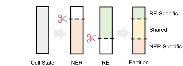
Figure 1: Partition process of cell neurons. Entity and relation gate are used to divide neurons into taskrelated and task-unrelated ones. Neurons relating to both tasks form the shared partition while the rest form two task partitions.
图 1: 细胞神经元划分过程。通过实体门控和关系门控将神经元划分为任务相关与任务无关两类。同时关联两个任务的神经元构成共享分区,其余神经元形成两个任务专属分区。
Conventionally, Named Entity Recognition (NER) and Relation Extraction (RE) are performed in a pipelined manner (Zelenko et al., 2002; Chan and Roth, 2011). These approaches are flawed in that they do not consider the intimate connection between NER and RE. Also, error propagation is another drawback of pipeline methods. In order to conquer these issues, joint extracting entity and relation is proposed and demonstrates stronger performance on both tasks. In early work, joint methods mainly rely on elaborate feature engineering to establish interaction between NER and RE (Yu and Lam, 2010; Li and Ji, 2014; Miwa and Sasaki, 2014). Recently, end-to-end neural network has shown to be successful in extracting relational triples (Zeng et al., 2014; Gupta et al., 2016; Katiyar and Cardie, 2017; Shen et al., 2021) and has since become the mainstream of joint entity and relation extraction.
传统上,命名实体识别(NER)和关系抽取(RE)以流水线方式执行 (Zelenko et al., 2002; Chan and Roth, 2011)。这些方法的缺陷在于未考虑NER与RE之间的紧密联系,且错误传播是流水线方法的另一弊端。为解决这些问题,联合抽取实体与关系的方法被提出,并在两项任务上展现出更强性能。早期工作中,联合方法主要依赖精心设计的特征工程来建立NER与RE间的交互 (Yu and Lam, 2010; Li and Ji, 2014; Miwa and Sasaki, 2014)。近年来,端到端神经网络在关系三元组抽取中取得成功 (Zeng et al., 2014; Gupta et al., 2016; Katiyar and Cardie, 2017; Shen et al., 2021),并由此成为联合实体关系抽取的主流方法。
According to their differences in encoding taskspecific features, most of the existing methods can be divided into two categories: sequential encoding and parallel encoding. In sequential encoding, task-specific features are generated sequentially, which means features extracted first are not affected by those that are extracted later. Zeng et al. (2018) and Wei et al. (2020) are typical examples of this category. Their methods extract features for different tasks in a predefined order. In parallel encoding, task-specific features are generated independently using shared input. Compared with sequential encoding, models build on this scheme do not need to worry about the implication of encoding order. For example, Fu et al. (2019) encodes entity and relation information separately using common features derived from their GCN encoder. Since both taskspecific features are extracted through isolated submodules, this approach falls into the category of parallel encoding.
根据编码任务特定特征方式的不同,现有方法主要可分为两类:顺序编码与并行编码。顺序编码中任务特征按序生成,即先提取的特征不受后续特征影响。Zeng等(2018) 和Wei等(2020) 是该类方法的典型代表,他们按预定义顺序为不同任务提取特征。并行编码则通过共享输入独立生成各任务特征,相比顺序编码,基于此方案的模型无需考虑编码顺序的影响。例如Fu等(2019) 利用GCN编码器生成的公共特征分别编码实体和关系信息,由于两个任务特征均通过独立子模块提取,该方法属于并行编码范畴。
However, both encoding designs above fail to model two-way interaction between NER and RE tasks properly. In sequential encoding, interaction is only unidirectional with a specified order, resulting in different amount of information exposed to NER and RE task. In parallel encoding, although encoding order is no longer a concern, interaction is only present in input sharing. Considering adding two-way interaction in feature encoding, we adopt an alternative encoding design: joint encoding. This design encodes task-specific features jointly with a single encoder where there should exist some mutual section for inter-task communication.
然而,上述两种编码设计都未能正确建模命名实体识别(NER)与关系抽取(RE)任务间的双向交互。在顺序编码中,交互仅按指定顺序单向进行,导致NER和RE任务获取的信息量不对等。并行编码虽消除了顺序限制,但交互仅体现在输入共享层面。为在特征编码中引入双向交互,我们采用了联合编码方案:通过单一编码器联合生成任务专属特征,并保留特征间的公共交互区域以实现跨任务通信。
In this work, we instantiate joint encoding with a partition filter encoder. Our encoder first sorts and partitions each neuron according to its contribution to individual tasks with entity and relation gates. During this process, two task partitions and one shared partition are formed (see figure 1). Then individual task partitions and shared partition are combined to generate task-specific features, filtering out irrelevant information stored in the opposite task partition.
在本工作中,我们通过分区过滤器编码器实现了联合编码。该编码器首先利用实体门和关系门,根据神经元对各个任务的贡献度进行排序和分区。此过程会形成两个任务分区和一个共享分区(见图1)。随后将独立任务分区与共享分区组合生成任务专属特征,同时过滤掉存储在对立任务分区中的无关信息。
Task interaction in our encoder is achieved in two ways: First, the partitions, especially the taskspecific ones, are formed through concerted efforts of entity and relation gates, allowing for interaction between the formation of entity and relation features determined by these partitions. Second, the shared partition, which represents information useful to both task, is equally accessible to the formation of both task-specific features, ensuring balanced two-way interaction. The contributions of our work are summarized below:
我们编码器中的任务交互通过两种方式实现:首先,分区(特别是任务特定分区)通过实体门和关系门的协同作用形成,使得由这些分区决定的实体特征与关系特征在形成过程中能够交互。其次,共享分区代表对两个任务都有用的信息,它可以平等地参与两个任务特定特征的形成,从而确保双向交互的平衡。我们工作的贡献总结如下:
- We propose partition filter network, a framework designed specifically for joint encoding. This method is capable of encoding taskspecific features and guarantees proper twoway interaction between NER and RE.
- 我们提出分区过滤网络 (partition filter network),这是一个专为联合编码设计的框架。该方法能够编码任务特定特征,并确保命名实体识别 (NER) 和关系抽取 (RE) 之间的双向交互。
- We conduct extensive experiments on six datasets. The main results show that our method is superior to other baseline approaches, and the ablation study provides insight into what works best for our framework.
- 我们在六个数据集上进行了大量实验。主要结果表明,我们的方法优于其他基线方法,消融研究深入揭示了框架中最有效的设计要素。
- Contrary to what previous work has claimed, our auxiliary experiments suggest that relation prediction is contributory to named entity prediction in a non-negligible way.
- 与先前研究结论相反,我们的辅助实验表明关系预测对命名实体预测的贡献不可忽视。
2 Related Work
2 相关工作
In recent years, joint entity and relation extraction approaches have been focusing on tackling triple overlapping problem and modelling task interaction. Solutions to these issues have been explored in recent works (Zheng et al., 2017; Zeng et al., 2018, 2019; Fu et al., 2019; Wei et al., 2020). The triple overlapping problem refers to triples sharing the same entity (SEO, i.e. Single Entity Overlap) or entities (EPO, i.e. Entity Pair Overlap). For example, In "Adam and Joe were born in the USA", since triples (Adam, birthplace, USA) and (Joe, birthplace, USA) share only one entity "USA", they should be categorized as SEO triples; or in "Adam was born in the USA and lived there ever since", triples (Adam, birthplace, USA) and (Adam, residence, USA) share both entities at the same time, thus should be categorized as EPO triples. Generally, there are two ways in tackling the problem. One is through generative methods like seq2seq (Zeng et al., 2018, 2019) where entity and relation mentions can be decoded multiple times in output sequence, another is by modeling each relation separately with sequences (Wei et al., 2020), graphs (Fu et al., 2019) or tables (Wang and Lu, 2020). Our method uses relation-specific tables (Miwa and Sasaki, 2014) to handle each relation separately.
近年来,联合实体与关系抽取方法主要聚焦于解决三元组重叠问题及建模任务交互。针对这些问题的解决方案已在近期研究中得到探索 (Zheng et al., 2017; Zeng et al., 2018, 2019; Fu et al., 2019; Wei et al., 2020)。三元组重叠问题指共享同一实体(SEO,即单实体重叠)或多个实体(EPO,即实体对重叠)的三元组。例如在"Adam和Joe都出生于美国"中,由于三元组(Adam,出生地,美国)和(Joe,出生地,美国)仅共享实体"美国",应归类为SEO三元组;而在"Adam出生于美国并一直居住于此"中,三元组(Adam,出生地,美国)和(Adam,居住地,美国)同时共享两个实体,故应归类为EPO三元组。现有解决方案主要分为两类:一类采用seq2seq等生成式方法 (Zeng et al., 2018, 2019),通过在输出序列中多次解码实体和关系提及;另一类则通过序列 (Wei et al., 2020)、图结构 (Fu et al., 2019) 或表格 (Wang and Lu, 2020) 分别建模每种关系。本方法采用关系专用表格 (Miwa and Sasaki, 2014) 来实现关系的独立处理。
Task interaction modeling, however, has not been well handled by most of the previous work. In some of the previous approaches, Task interaction is achieved with entity and relation prediction sharing the same features (Tran and Kavuluru, 2019; Wang et al., 2020b). This could be problematic as information about entity and relation could sometimes be contradictory. Also, as models that use sequential encoding (Bekoulis et al., 2018b; Eberts and Ulges, 2019; Wei et al., 2020) or parallel encoding (Fu et al., 2019) lack proper two-way interaction in feature extraction, predictions made on these features suffer the problem of improper interaction. In our work, the partition filter encoder is built on joint encoding and is capable of handling communication of inter-task information more appropriately to avoid the problem of sequential and parallel encoding (exposure bias and insufficient interaction), while keeping intra-task information away from the opposite task to mitigate the problem of negative transfer between the tasks.
然而,任务交互建模在多数先前工作中并未得到妥善处理。部分早期方法通过实体与关系预测共享相同特征来实现任务交互 (Tran and Kavuluru, 2019; Wang et al., 2020b),这种做法存在隐患,因为实体与关系信息有时可能相互矛盾。此外,采用序列编码 (Bekoulis et al., 2018b; Eberts and Ulges, 2019; Wei et al., 2020) 或并行编码 (Fu et al., 2019) 的模型由于特征提取阶段缺乏适当的双向交互,基于这些特征的预测会存在交互不当的问题。本研究提出的分区过滤器编码器基于联合编码构建,能更合理地处理任务间信息交流,既避免了序列/并行编码的暴露偏差和交互不足问题,又通过隔离任务内信息来减轻任务间负迁移的影响。
3 Problem Formulation
3 问题表述
Our framework split up joint entity and relation extraction into two sub-tasks: NER and RE. Formally, Given an input sequence $s={w_{1},\dots,w_{L}}$ with $L$ tokens, $w_{i}$ denotes the i-th token in sequence $s$ . For NER, we aim to extract all typed entities whose set is denoted as $S$ , where $\langle w_{i},e,w_{j}\rangle\in S$ signifies that token $w_{i}$ and $w_{j}$ are the start and end token of an entity typed $e\in\mathcal{E}$ . $\mathcal{E}$ represents the set of entity types. Concerning RE, the goal is to identify all head-only triples whose set is denoted as $T$ , each triple $\langle w_{i},r,w_{j}\rangle\in T$ indicates that tokens $w_{i}$ and $w_{j}$ are the corresponding start token of subject and object entity with relation $r\in\mathcal{R}$ . $\mathcal{R}$ represents the set of relation types. Combining the results from both NER and RE, we should be able to extract relational triples with complete entity spans.
我们的框架将联合实体和关系抽取拆分为两个子任务:NER(命名实体识别)和RE(关系抽取)。形式化地,给定一个输入序列 $s={w_{1},\dots,w_{L}}$(包含 $L$ 个token),$w_{i}$ 表示序列 $s$ 中的第i个token。对于NER任务,目标是抽取所有类型化实体,其集合记为 $S$,其中 $\langle w_{i},e,w_{j}\rangle\in S$ 表示token $w_{i}$ 和 $w_{j}$ 是一个类型为 $e\in\mathcal{E}$ 的实体的起始和结束token,$\mathcal{E}$ 代表实体类型集合。对于RE任务,目标是识别所有头实体三元组,其集合记为 $T$,每个三元组 $\langle w_{i},r,w_{j}\rangle\in T$ 表示token $w_{i}$ 和 $w_{j}$ 分别是具有关系 $r\in\mathcal{R}$ 的主客体实体的起始token,$\mathcal{R}$ 表示关系类型集合。结合NER和RE的结果,我们就能抽取具有完整实体跨度的关系三元组。
4 Model
4 模型
We describe our model design in this section. Our model consists of a partition filter encoder and two task units, namely NER unit and RE unit. The partition filter encoder is used to generate taskspecific features, which will be sent to task units as input for entity and relation prediction. We will discuss each component in detail in the following three sub-sections.
在本节中,我们将描述模型设计。我们的模型由分区过滤器编码器和两个任务单元组成,即命名实体识别(NER)单元和关系抽取(RE)单元。分区过滤器编码器用于生成任务特定特征,这些特征将作为输入发送至任务单元以进行实体和关系预测。我们将在以下三个子章节中详细讨论每个组件。
4.1 Partition Filter Encoder
4.1 分区过滤器编码器
Similar to LSTM, the partition filter encoder is a recurrent feature encoder with information stored in intermediate memories. In each time step, the encoder first divides neurons into three partitions: entity partition, relation partition and shared partition. Then it generates task-specific features by selecting and combining these partitions, filtering out information irrelevant to each task. As shown in figure 2, this module is designed specifically to jointly extract task-specific features, which strictly follows two steps: partition and filter.
与LSTM类似,分区过滤器编码器是一种具有中间记忆存储的循环特征编码器。在每个时间步中,编码器首先将神经元划分为三个分区:实体分区、关系分区和共享分区。然后通过选择和组合这些分区来生成任务特定特征,过滤掉与每个任务无关的信息。如图2所示,该模块专为联合提取任务特定特征而设计,严格遵循两个步骤:分区和过滤。
Partition This step performs neuron partition to divide cell neurons into three partitions: Two task partitions storing intra-task information, namely entity partition and relation partition, as well as one shared partition storing inter-task information. The neuron to be divided are candidate cell $\tilde{c}{t}$ representing current information and previous cell $c_{t-1}$ representing history information. $c_{t-1}$ is the direct input from the last time step and $\tilde{c}_{t}$ is calculated in the same manner as LSTM:
分区
此步骤执行神经元分区,将单元神经元划分为三个分区:两个存储任务内信息的任务分区,即实体分区和关系分区,以及一个存储任务间信息的共享分区。待划分的神经元是表示当前信息的候选单元$\tilde{c}{t}$和表示历史信息的先前单元$c_{t-1}$。$c_{t-1}$是来自上一时间步的直接输入,而$\tilde{c}_{t}$的计算方式与LSTM相同:
$$
\tilde{c}{t}=\operatorname{tanh}(\operatorname{Linear}(\left[x_{t};h_{t-1}\right]))
$$
$$
\tilde{c}{t}=\operatorname{tanh}(\operatorname{Linear}(\left[x_{t};h_{t-1}\right]))
$$
where Linear stands for the operation of linear transformation.
Linear代表线性变换操作。
We leverage entity gate $\tilde{e}$ and relation gate $\tilde{r}$ , which are referred to as master gates in (Shen et al., 2019), for neuron partition. As illustrated in figure 1, each gate, which represents one specific task, will divide neurons into two segments according to their usefulness to the designated task. For example, entity gate $\tilde{e}$ will separate neurons into two partitions: NER-related and NER-unrelated. The shared partition is formed by combining partition results from both gates. Neurons in the shared partition can be regarded as information valuable to both tasks. In order to model twoway interaction properly, inter-task information in the shared partition is evenly accessible to both tasks (which will be discussed in the filter subsection). In addition, information valuable to only one task is invisible to the opposing task and will be stored in individual task partitions. The gates are calculated using cummax activation function cummax $(\cdot)=c u m s u m(s o f t m a x(\cdot))^{1}$ , whose output can be seen as approximation of a binary gate with the form of $(0,\ldots,0,1,\ldots,1)$ :
我们利用实体门 $\tilde{e}$ 和关系门 $\tilde{r}$ (在 Shen et al., 2019 中称为主门) 进行神经元划分。如图 1 所示,每个代表特定任务的门会根据神经元对指定任务的有用性将其划分为两个部分。例如,实体门 $\tilde{e}$ 会将神经元分为两个分区:与 NER 相关和与 NER 无关。共享分区是通过合并两个门的划分结果形成的。共享分区中的神经元可视为对两个任务都有价值的信息。为了正确建模双向交互,共享分区中的跨任务信息对两个任务都是平等可访问的 (这将在过滤器小节中讨论)。此外,仅对单个任务有价值的信息对另一个任务不可见,并将存储在各自的任务分区中。门的计算使用 cummax 激活函数 cummax $(\cdot)=c u m s u m(s o f t m a x(\cdot))^{1}$,其输出可视为形式为 $(0,\ldots,0,1,\ldots,1)$ 的二元门近似。
$$
\begin{array}{r l}&{\tilde{e}=\mathrm{cummax}(\mathrm{Linear}([x_{t};h_{t-1}]))}\ &{\tilde{r}=1-\mathrm{cummax}(\mathrm{Linear}([x_{t};h_{t-1}]))}\end{array}
$$
$$
\begin{array}{r l}&{\tilde{e}=\mathrm{cummax}(\mathrm{Linear}([x_{t};h_{t-1}]))}\ &{\tilde{r}=1-\mathrm{cummax}(\mathrm{Linear}([x_{t};h_{t-1}]))}\end{array}
$$
The intuition behind equation (2) is to identify two cut-off points, displayed as scissors in figure 2, which naturally divide a set of neurons into three segments.
方程 (2) 背后的直觉是找出两个截断点,如图 2 中的剪刀所示,它们自然地将一组神经元分成三个部分。
As a result, the gates will divide neurons into three partitions, entity partition $\rho_{e}$ , relation partition $\rho_{r}$ and shared partition $\rho_{s}$ . Partitions for previous cell ct 1 are formulated as below: 2
因此,门控机制会将神经元划分为三个分区:实体分区 $\rho_{e}$、关系分区 $\rho_{r}$ 和共享分区 $\rho_{s}$。前一个细胞 ct 1 的分区公式如下:2
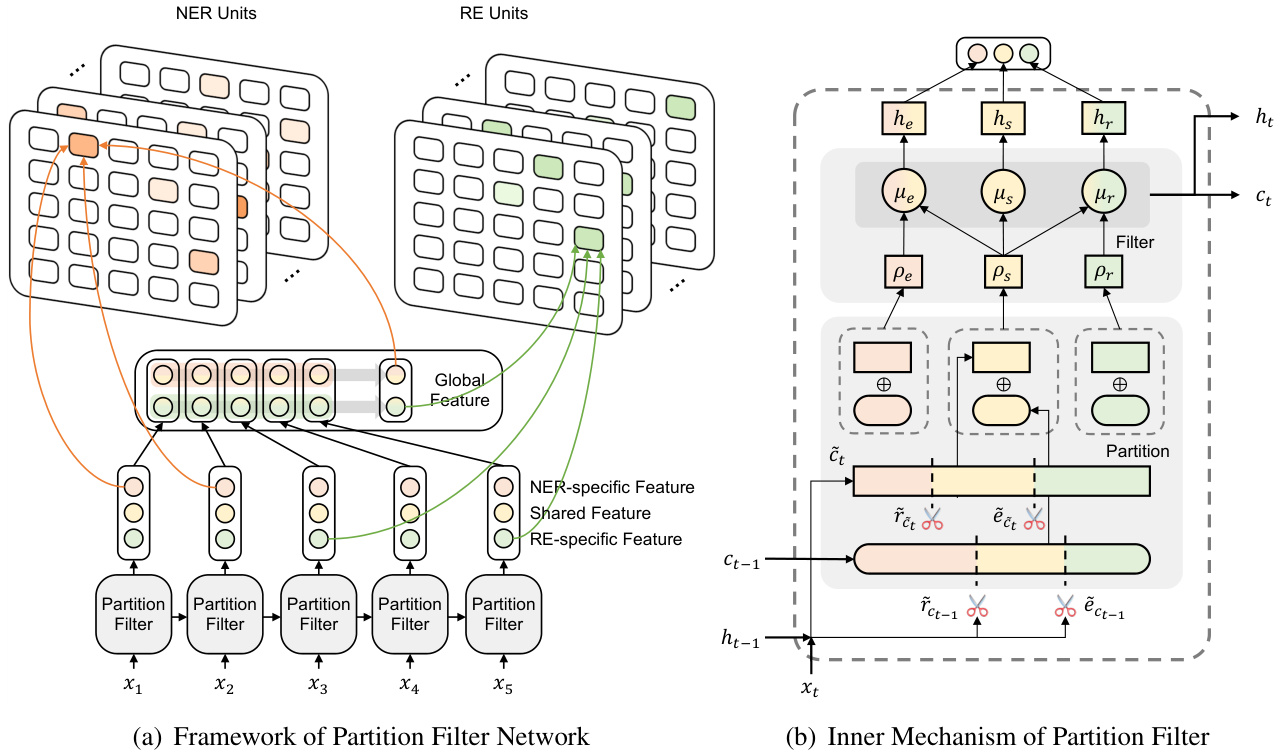
Figure 2: (a) Overview of PFN. The framework consists of three components: partition filter encoder, NER unit and RE unit. In task units, we use table-filling for word pair prediction. Orange, yellow and green represents NER-related, shared and RE-related component or features. (b) Detailed depiction of partition filter encoder in one single time step. We decompose feature encoding into two steps: partition and filter (shown in the gray area). In partition, we first segment neurons into two task partitions and one shared partition. Then in filter, partitions are selected and combined to form task-specific features and shared features, filtering out information irrelevant to each task.
图 2: (a) PFN框架概览。该框架包含三个组件: 分区过滤器编码器、NER单元和RE单元。在任务单元中, 我们使用表格填充(word pair prediction)进行预测。橙色、黄色和绿色分别代表NER相关、共享以及RE相关的组件或特征。(b) 单时间步内分区过滤器编码器的详细结构。我们将特征编码分解为两个步骤: 分区(partition)和过滤(filter)(如灰色区域所示)。在分区步骤中, 我们首先将神经元划分为两个任务分区和一个共享分区。然后在过滤步骤中, 通过选择并组合分区来形成任务特定特征和共享特征, 同时过滤掉与各任务无关的信息。
$$
\begin{array}{r l}&{\rho_{s,c_{t-1}}=\tilde{e}{c_{t-1}}\circ\tilde{r}{c_{t-1}}}\ &{\rho_{e,c_{t-1}}=\tilde{e}{c_{t-1}}-\rho_{s,c_{t-1}}}\ &{\rho_{r,c_{t-1}}=\tilde{r}{c_{t-1}}-\rho_{s,c_{t-1}}}\end{array}
$$
$$
\begin{array}{r l}&{\rho_{s,c_{t-1}}=\tilde{e}{c_{t-1}}\circ\tilde{r}{c_{t-1}}}\ &{\rho_{e,c_{t-1}}=\tilde{e}{c_{t-1}}-\rho_{s,c_{t-1}}}\ &{\rho_{r,c_{t-1}}=\tilde{r}{c_{t-1}}-\rho_{s,c_{t-1}}}\end{array}
$$
Note that if you add up all three partitions, the result is not equal to one. This guarantees that in forward message passing, some information is discarded to ensure that message is not overloaded, which is similar to the forgetting mechanism in LSTM.
需要注意的是,如果将三个分区的值相加,结果并不等于1。这保证了在前向消息传递过程中会丢弃部分信息,以防止消息过载,类似于LSTM中的遗忘机制。
Then, we aggregate partition information from both target cells, and three partitions are formed as a result. For all three partitions, we add up all related information from both cells:
然后,我们汇总来自两个目标单元格的分区信息,最终形成三个分区。对于这三个分区,我们将两个单元格中的所有相关信息相加:
$$
\begin{array}{r}{\rho_{e}=\rho_{e,c_{t-1}}\circ c_{t-1}+\rho_{e,\tilde{c}{t}}\circ\tilde{c}{t}}\ {\rho_{r}=\rho_{r,c_{t-1}}\circ c_{t-1}+\rho_{r,\tilde{c}{t}}\circ\tilde{c}{t}}\ {\rho_{s}=\rho_{s,c_{t-1}}\circ c_{t-1}+\rho_{s,\tilde{c}{t}}\circ\tilde{c}_{t}}\end{array}
$$
$$
\begin{array}{r}{\rho_{e}=\rho_{e,c_{t-1}}\circ c_{t-1}+\rho_{e,\tilde{c}{t}}\circ\tilde{c}{t}}\ {\rho_{r}=\rho_{r,c_{t-1}}\circ c_{t-1}+\rho_{r,\tilde{c}{t}}\circ\tilde{c}{t}}\ {\rho_{s}=\rho_{s,c_{t-1}}\circ c_{t-1}+\rho_{s,\tilde{c}{t}}\circ\tilde{c}_{t}}\end{array}
$$
Filter We propose three types of memory block: entity memory, relation memory and shared memory. Here we denote $\mu_{e}$ as entity memory, $\mu_{r}$ as relation memory and $\mu_{s}$ as shared memory. In $\mu_{e}$ , information in entity partition and shared partition are selected. In contrast, information in relation partition, which we assume is irrelevant or even harmful to named entity recognition task, is filtered out. The same logic applies to $\mu_{r}$ as well, where information in entity partition is filtered out and the rest is kept. In addition, information in shared partition will be stored in $\mu_{s}$ :
我们提出了三种类型的内存块:实体记忆 (entity memory) 、关系记忆 (relation memory) 和共享记忆 (shared memory) 。这里我们将 $\mu_{e}$ 表示为实体记忆, $\mu_{r}$ 表示为关系记忆, $\mu_{s}$ 表示为共享记忆。在 $\mu_{e}$ 中,实体分区和共享分区中的信息被选中。相反,我们假设关系分区中的信息对命名实体识别任务无关甚至有害,因此被过滤掉。同样的逻辑也适用于 $\mu_{r}$ ,其中实体分区中的信息被过滤掉,其余部分被保留。此外,共享分区中的信息将存储在 $\mu_{s}$ 中:
$$
\mu_{e}=\rho_{e}+\rho_{s};\mu_{r}=\rho_{r}+\rho_{s};\mu_{s}=\rho_{s}
$$
$$
\mu_{e}=\rho_{e}+\rho_{s};\mu_{r}=\rho_{r}+\rho_{s};\mu_{s}=\rho_{s}
$$
Note that inter-task information in the shared partition is accessible to both entity memory and relation memory, allowing balanced interaction between NER and RE. Whereas in sequential and parallel encoding, relation features have no direct impact on the formation of entity features.
请注意,共享分区中的任务间信息对实体记忆和关系记忆都是可访问的,这允许命名实体识别(NER)和关系抽取(RE)之间实现平衡的交互。而在顺序编码和并行编码中,关系特征对实体特征的形成没有直接影响。
After updating information in each memory, entity features $h_{e}$ , relation features $h_{r}$ and shared features $h_{s}$ are generated with corresponding memories:
在每次更新记忆信息后,会生成实体特征 $h_{e}$、关系特征 $h_{r}$ 和共享特征 $h_{s}$,它们分别对应不同的记忆模块:
$$
\begin{array}{r}{h_{e}=\operatorname{tanh}(\mu_{e})}\ {h_{r}=\operatorname{tanh}(\mu_{r})}\ {h_{s}=\operatorname{tanh}(\mu_{s})}\end{array}
$$
$$
\begin{array}{r}{h_{e}=\operatorname{tanh}(\mu_{e})}\ {h_{r}=\operatorname{tanh}(\mu_{r})}\ {h_{s}=\operatorname{tanh}(\mu_{s})}\end{array}
$$
Following the partition and filter steps, information in all three memories is used to form cell state $c_{t}$ , which will then be used to generate hidden state $h_{t}$ (The hidden and cell state at time step $t$ are input to the next time step):
在完成分区和过滤步骤后,所有三个记忆单元中的信息被用于形成细胞状态 $c_{t}$ ,随后该状态将用于生成隐藏状态 $h_{t}$ (时间步 $t$ 的隐藏状态和细胞状态将作为下一时间步的输入):
$$
\begin{array}{r l}&{c_{t}=\operatorname{Linear}([\mu_{e,t};\mu_{r,t};\mu_{s,t}])}\ &{h_{t}=\operatorname{tanh}(c_{t})}\end{array}
$$
$$
\begin{array}{r l}&{c_{t}=\operatorname{Linear}([\mu_{e,t};\mu_{r,t};\mu_{s,t}])}\ &{h_{t}=\operatorname{tanh}(c_{t})}\end{array}
$$
4.2 Global Representation
4.2 全局表征
In our model, we employ a unidirectional encoder for feature encoding. The backward encoder in the bidirectional setting is replaced with task-specific global representation to capture the semantics of future context. Empirically this shows to be more effective. For each task, global representation is the combination of task-specific features and shared features computed by:
在我们的模型中,我们采用单向编码器进行特征编码。双向设置中的反向编码器被替换为任务特定的全局表示,以捕捉未来上下文的语义。经验表明这种方法更为有效。对于每个任务,全局表示由任务特定特征和共享特征组合而成,计算方式如下:
$$
\begin{array}{r l}&{h_{g_{e},t}=\operatorname{tanh}(\operatorname{Linear}[h_{e,t};h_{s,t}])}\ &{h_{g_{r},t}=\operatorname{tanh}(\operatorname{Linear}[h_{r,t};h_{s,t}])}\ &{h_{g_{e}}=\operatorname*{maxpool}(h_{g_{e},1},\dots,h_{g_{e},L})}\ &{h_{g_{r}}=\operatorname{maxpool}(h_{g_{r},1},\dots,h_{g_{r},L})}\end{array}
$$
$$
\begin{array}{r l}&{h_{g_{e},t}=\operatorname{tanh}(\operatorname{Linear}[h_{e,t};h_{s,t}])}\ &{h_{g_{r},t}=\operatorname{tanh}(\operatorname{Linear}[h_{r,t};h_{s,t}])}\ &{h_{g_{e}}=\operatorname*{maxpool}(h_{g_{e},1},\dots,h_{g_{e},L})}\ &{h_{g_{r}}=\operatorname{maxpool}(h_{g_{r},1},\dots,h_{g_{r},L})}\end{array}
$$
4.3 Task Units
4.3 任务单元
Our model consists of two task units: NER unit and RE unit. In NER unit, the objective is to identify and categorize all entity spans in a given sentence. More specifically, the task is treated as a type-specific table filling problem. Given a entity type set $\mathcal{E}$ , for each type $k$ , we fill out a table whose element $e_{i j}^{k}$ represents probability of word $w_{i}$ and word $w_{j}$ being start and end position of an entity with type $k$ . For each word pair $(w_{i},w_{j})$ , we concatenate word-level entity featur e(s $h_{i}^{e}$ an)d $h_{j}^{e}$ as well as sentence-level global features $h_{g_{e}}$ before feeding it into a fully-connected layer with ELU activation to get entity span representation $h_{i j}^{e}$ :
我们的模型由两个任务单元组成:命名实体识别(NER)单元和关系抽取(RE)单元。在NER单元中,目标是识别并分类给定句子中的所有实体跨度。具体而言,该任务被视为类型特定的表格填充问题。给定实体类型集合$\mathcal{E}$,对于每个类型$k$,我们填充一个表格,其元素$e_{i j}^{k}$表示单词$w_{i}$和单词$w_{j}$作为类型$k$实体起止位置的概率。对于每个词对$(w_{i},w_{j})$,我们将词级实体特征$h_{i}^{e}$和$h_{j}^{e}$与句子级全局特征$h_{g_{e}}$拼接后,输入带有ELU激活函数的全连接层以获得实体跨度表示$h_{i j}^{e}$:
$$
h_{i j}^{e}=\mathrm{ELU}(\mathrm{Linear}([h_{i}^{e};h_{j}^{e};h_{g e}]))
$$
$$
h_{i j}^{e}=\mathrm{ELU}(\mathrm{Linear}([h_{i}^{e};h_{j}^{e};h_{g e}]))
$$
With the span representation, we can predict whether the span is an entity with type $k$ by feeding it into a feed forward neural layer:
通过跨度表示,我们可以将其输入前馈神经网络层来预测该跨度是否为类型 $k$ 的实体:
$$
\begin{array}{r}{e_{i j}^{k}=p\big(e=\langle w_{i},k,w_{j}\rangle|e\in S\big)}\ {=\sigma\big(\mathrm{Linear}(h_{i j}^{e})\big),\forall k\in\mathcal{E}}\end{array}
$$
$$
\begin{array}{r}{e_{i j}^{k}=p\big(e=\langle w_{i},k,w_{j}\rangle|e\in S\big)}\ {=\sigma\big(\mathrm{Linear}(h_{i j}^{e})\big),\forall k\in\mathcal{E}}\end{array}
$$
where $\sigma$ represents sigmoid activation function.
其中 $\sigma$ 表示 sigmoid 激活函数。
Computation in RE unit is mostly symmetrical to NER unit. Given a set of gold relation triples denoted as $T$ , this unit aims to identify all triples in the sentence. We only predict starting word of each entity in this unit as entity span prediction is already covered in NER unit. Similar to NER, we consider relation extraction as a relation-specific table filling problem. Given a relation label set $\mathcal{R}$ , for each relation $l\in\mathcal{R}$ , we fill out a table whose element $r_{i j}^{l}$ represents the probability of word $w_{i}$ and word $w_{j}$ being starting word of subject and object entity. In this way, we can extract all triples revolving around relation $l$ with one relation table. For each triple $(w_{i},l,w_{j})$ , similar to NER unit, triple representation $h_{i j}^{r}$ and relation score $r_{i j}^{l}$ are calculated as follows:
RE (关系抽取) 单元的计算过程与NER (命名实体识别) 单元基本对称。给定一组标注好的关系三元组$T$,该单元的目标是识别句子中的所有三元组。由于实体跨度预测已在NER单元完成,本单元仅预测每个实体的起始词。与NER类似,我们将关系抽取视为特定于关系类型的表格填充问题。给定关系标签集$\mathcal{R}$,对于每个关系$l\in\mathcal{R}$,我们填充一个表格,其元素$r_{i j}^{l}$表示词$w_{i}$与词$w_{j}$分别作为主体和客体实体起始词的概率。通过这种方式,我们可以用一个关系表提取围绕关系$l$的所有三元组。对于每个三元组$(w_{i},l,w_{j})$,与NER单元类似,三元组表示$h_{i j}^{r}$和关系分数$r_{i j}^{l}$的计算方式如下:
$$
\begin{array}{r l}&{h_{i j}^{r}=\mathrm{ELU}(\mathrm{Linear}([h_{i}^{r};h_{j}^{r};h_{g r}]))}\ &{r_{i j}^{l}=p(r=\langle w_{i},l,w_{j}\rangle|r\in T)}\ &{\quad\quad=\sigma(\mathrm{Linear}(h_{i j}^{r})),\forall l\in\mathcal{R}}\end{array}
$$
$$
\begin{array}{r l}&{h_{i j}^{r}=\mathrm{ELU}(\mathrm{Linear}([h_{i}^{r};h_{j}^{r};h_{g r}]))}\ &{r_{i j}^{l}=p(r=\langle w_{i},l,w_{j}\rangle|r\in T)}\ &{\quad\quad=\sigma(\mathrm{Linear}(h_{i j}^{r})),\forall l\in\mathcal{R}}\end{array}
$$
4.4 Training and Inference
4.4 训练与推理
For a given training dataset, the loss function $L$ that guides the model during training consists of two parts: $L_{n e r}$ for NER unit and $L_{r e}$ for RE unit:
对于给定的训练数据集,指导模型训练的损失函数 $L$ 由两部分组成:NER单元的 $L_{ner}$ 和RE单元的 $L_{re}$:
$$
\begin{array}{r l}&{L_{n e r}=\sum_{\hat{e}{i j}^{k}\in S}\mathrm{BCELoss}(e_{i j}^{k},\hat{e}{i j}^{k})}\ &{L_{r e}=\sum_{\hat{r}{i j}^{l}\in T}\mathrm{BCELoss}(r_{i j}^{l},\hat{r}_{i j}^{l})}\end{array}
$$
$$
\begin{array}{r l}&{L_{n e r}=\sum_{\hat{e}{i j}^{k}\in S}\mathrm{BCELoss}(e_{i j}^{k},\hat{e}{i j}^{k})}\ &{L_{r e}=\sum_{\hat{r}{i j}^{l}\in T}\mathrm{BCELoss}(r_{i j}^{l},\hat{r}_{i j}^{l})}\end{array}
$$
$\hat{e}{i j}^{k}$ and $\hat{r}{i j}^{l}$ are respectively ground truth label of entity table and relation table. $e_{i j}^{k}$ and rl are the predicted ones. We adopt BCELoss for each task3. The training objective is to minimize the loss function $L$ , which is computed as $L_{n e r}+L_{r e}$ .
$\hat{e}{i j}^{k}$ 和 $\hat{r}{i j}^{l}$ 分别是实体表和关系表的真实标签。$e_{i j}^{k}$ 和 rl 是预测值。我们对每个任务采用 BCELoss。训练目标是最小化损失函数 $L$,其计算方式为 $L_{n e r}+L_{r e}$。
During inference, we extract relational triples by combining results from both NER and RE unit. For each legitimate triple prediction $(s_{i,j}^{k},l,o_{m,n}^{k^{\prime}})$ where $l$ is the relation label, $k$ and $k^{\prime}$ are the entity type labels, and the indexes $i,j$ and $m,n$ are respectively starting and ending index of subject entity $s$ and object entity $o$ , the following conditions should be satisfied:
在推理过程中,我们通过结合命名实体识别(NER)和关系抽取(RE)单元的结果来提取关系三元组。对于每个合法的三元组预测 $(s_{i,j}^{k},l,o_{m,n}^{k^{\prime}})$ ,其中 $l$ 是关系标签, $k$ 和 $k^{\prime}$ 是实体类型标签,索引 $i,j$ 和 $m,n$ 分别表示主体实体 $s$ 和客体实体 $o$ 的起始和结束位置,需满足以下条件:
$$
e_{i j}^{k}\geq\lambda_{e};~e_{m n}^{k^{\prime}}\geq\lambda_{e};~r_{i m}^{l}\geq\lambda_{r}
$$
$$
e_{i j}^{k}\geq\lambda_{e};~e_{m n}^{k^{\prime}}\geq\lambda_{e};~r_{i m}^{l}\geq\lambda_{r}
$$
$\lambda_{e}$ and $\lambda_{r}$ are threshold hyper-parameters for entity and relation prediction, both set to be 0.5 without further fine-tuning.
$\lambda_{e}$ 和 $\lambda_{r}$ 是实体预测和关系预测的阈值超参数,均设为0.5且未进一步微调。
5 Experiment
5 实验
5.1 Dataset, Evaluation and Implementation Details
5.1 数据集、评估与实现细节
We evaluate our model on six datasets. NYT (Riedel et al., 2010), WebNLG (Zeng et al., 2018),
我们在六个数据集上评估了模型。NYT (Riedel et al., 2010)、WebNLG (Zeng et al., 2018)
ADE (Gu ruling appa et al., 2012), SciERC (Luan et al., 2018), ACE04 and ACE05 (Walker et al., 2006). Descriptions of the datasets can be found in Appendix A.
ADE (Gu等人, 2012)、SciERC (Luan等人, 2018)、ACE04和ACE05 (Walker等人, 2006)。数据集的详细说明见附录A。
Following previous work, we assess our model on NYT/WebNLG under partial match, where only the tail of an entity is annotated. Besides, as entity type information is not annotated in these datasets, we set the type of all entities to a single label "NONE", so entity type would not be predicted in our model. On ACE05, ACE04, ADE and SciERC, we assess our model under exact match where both head and tail of an entity are annotated. For ADE and ACE04, 10-fold and 5- fold cross validation are used to evaluate the model respectively, and $15%$ of the training set is used to construct the development set. For evaluation metrics, we report F1 scores in both NER and RE. In NER, an entity is seen as correct only if its type and boundary are correct. In RE, A triple is correct only if the types, boundaries of both entities and their relation type are correct. In addition, we report Macro-F1 score in ADE and Micro-F1 score in other datasets.
遵循先前工作,我们在NYT/WebNLG数据集上采用部分匹配(partial match)评估模型性能,其中仅标注实体的尾部信息。此外,由于这些数据集未标注实体类型信息,我们将所有实体类型统一设为"NONE"标签,因此模型不会预测实体类型。在ACE05、ACE04、ADE和SciERC数据集上,我们采用精确匹配(exact match)评估模型性能,要求同时标注实体的首尾边界。对于ADE和ACE04数据集,分别采用10折和5折交叉验证进行评估,并抽取训练集的15%构建开发集。评估指标方面,我们同时报告命名实体识别(NER)和关系抽取(RE)的F1值:NER任务中,仅当实体类型与边界均正确时判定为正确;RE任务中,仅当两个实体的类型/边界及其关系类型全部正确时判定三元组正确。另需说明,ADE数据集采用Macro-F1指标,其他数据集采用Micro-F1指标。
We choose our model parameters based on the performance in the development set (the best average F1 score of NER and RE) and report the results on the test set. More details of hyperparameters can be found in Appendix B
我们根据开发集上的性能(命名实体识别(NER)和关系抽取(RE)的最佳平均F1分数)选择模型参数,并在测试集上报告结果。更多超参数细节可参见附录B。
5.2 Main Result
5.2 主要结果
Table 1 shows the comparison of our model with existing approaches. In partially annotated datasets WebNLG and NYT, under the setting of BERT. For RE, our model achieves $1.7%$ improvement in WebNLG but performance in NYT is only slightly better than previous SOTA TpLinker (Wang et al., 2020b) by $0.5%$ margin. We argue that this is because NYT is generated with distant supervision, and annotation for entity and relation are often incomplete and wrong. Compared to TpLinker, the strength of our method is to reinforce two-way interaction between entity and relation. However, when dealing with noisy data, the strength might be counter-productive as error propagation between both tasks is amplified as well.
表 1: 展示了我们的模型与现有方法的对比结果。在部分标注数据集 WebNLG 和 NYT 上,基于 BERT 的设置下。对于关系抽取 (RE) 任务,我们的模型在 WebNLG 上实现了 1.7% 的性能提升,但在 NYT 上的表现仅比之前的 SOTA 方法 TpLinker (Wang et al., 2020b) 高出 0.5%。我们认为这是因为 NYT 是通过远程监督生成的,实体和关系的标注往往不完整且存在错误。与 TpLinker 相比,我们方法的优势在于加强了实体和关系之间的双向交互。然而,在处理噪声数据时,这种优势可能会适得其反,因为两个任务之间的错误传播也会被放大。
For NER, our method shows a distinct advantage over baselines that report the figures. Compared to Casrel (Wei et al., 2020), a competitive method, our F1 scores are $2.3%/2.5%$ higher in NYT/WebNLG. This proves that exposing relation information to
在命名实体识别(NER)任务中,我们的方法相较于已公布数据的基线模型展现出明显优势。与竞争方法Casrel (Wei et al., 2020)相比,我们的F1分数在NYT/WebNLG数据集上分别高出$2.3%/2.5%$。这证明将关系信息显式地
| 方法 | NER | RE |
|---|---|---|
| NYT △ | ||
| CopyRE (Zeng et al., 2018) | 86.2 | 58.7 |
| GraphRel (Fu et al.,2019) | 89.2 | 61.9 |
| CopyRL (Zeng et al., 2019) | 72.1 | |
| Casrel (Wei et al., 2020) | (93.5) | 89.6 |
| TpLinker (Wang et al., 2020b) | 91.9 | |
| PFN' | 95.8 | 92.4 |
| WebNLG△ | ||
| CopyRE (Zeng et al.,2018) | 82.1 | 37.1 |
| GraphRel (Fu et al.,2019) | 91.9 | 42.9 |
| CopyRL (Zeng et al., 2019) | 61.6 | |
| Casrel (Wei et al., 2020) | (95.5) | 91.8 |
| TpLinker (Wang et al., 2020b) | 91.9 | |
| PFN* | 98.0 | 93.6 |
| ADE | ||
| Multi-head (Bekoulis et al.,2018b) | 86.4 | 74.6 |
| Multi-head + AT (Bekoulis et al., 2018a) | 86.7 | 75.5 |
| Rel-Metric (Tran and Kavuluru, 2019) | 87.1 | 77.3 |
| SpERT (Eberts and Ulges, 2019) | 89.3 | 79.2 |
| Table-Sequence (Wang and Lu, 2020) | 89.7 | 80.1 |
| PFN' | 89.6 | 80.0 |
| PFN* | 91.3 | 83.2 |
| ACE05△ | ||
| Structured Perceptron (Li and Ji, 2014) | 80.8 | 49.5 |
| SPTree (Miwa andBansal,2016) | 83.4 | 55.6 |
| Multi-turn QA (Li et al.,2019) | 84.8 | 60.2 |
| Table-Sequence (Wang and Lu, 2020) | 89.5 | 64.3 |
| PURE (Zhong and Chen, 2021) | 89.7 | 65.6 |
| PFN* | 89.0 | 66.8 |
| ACE04 | ||
| Structured Perceptron (Li and Ji, 2014) | 79.7 | 45.3 |
| SPTree (Miwa and Bansal,2016) | 81.8 | 48.4 |
| Multi-turn QA (Li et al., 2019) | 83.6 | 49.4 |
| Table-Sequence (Wang and Lu, 2020) | 88.6 | 59.6 |
| PURE (Zhong and Chen, 2021) * | 88.8 | 60.2 |
| PFN* | 89.3 | 62.5 |
| SciERC△ | ||
| SPE (Wang et al.,2020a) | 68.0 | 34.6 |
| PURE (Zhong and Chen, 2021) | 66.6 | 35.6 |
| PFN$ | 66.8 | 38.4 |
Table 1: Experiment results on six datasets. † $^\ddagger$ and § denotes the use of BERT, ALBERT and SCIBERT(Devlin et al., 2019; Lan et al., 2020; Beltagy et al., 2019) pre-trained embedding. $\triangle$ and $\blacktriangle$ denotes the use of micro-F1 and macro-F1 score. NER results of Casrel are its reported average score of head and tail entity. Results of PURE are reported in single-sentence setting for fair comparison.
表 1: 六个数据集上的实验结果。† $^\ddagger$ 和 § 分别表示使用 BERT、ALBERT 和 SCIBERT (Devlin et al., 2019; Lan et al., 2020; Beltagy et al., 2019) 预训练嵌入。$\triangle$ 和 $\blacktriangle$ 分别表示使用 micro-F1 和 macro-F1 分数。Casrel 的 NER 结果为其报告的头尾实体平均分数。为公平比较,PURE 的结果在单句设置下报告。
NER, which is not present in Casrel, leads to better performance in entity recognition.
NER (在 Casrel 中未采用) 能提升实体识别性能。
Furthermore, our model demonstrates strong performance in fully annotated datasets ADE, ACE05, ACE04 and SciERC. For ADE, our model surpasses table-sequence (Wang and Lu, 2020) by $1.6%/3.1%$ in NER/RE. For ACE05, our model surpasses PURE (Zhong and Chen, 2021) by $1.2%$ in RE but results in weaker performance in NER by $0.7%$ . We argue that it could be attributed to the fact that, unlike the former three datasets, ACE05 contains many entities that do not belong to any triple. Thus utilizing relation information for entity prediction might not be as fruitful as that in other datasets (PURE is a pipeline approach where relation information is unseen to entity prediction). In ACE04, our model surpasses PURE by $0.5%/2.3%$ in NER/RE. In SciERC, our model surpasses PURE by $0.2%/2.8%$ in NER/RE. Overall, the performance of our model shows remarkable improvement against previous baselines.
此外,我们的模型在完全标注的数据集ADE、ACE05、ACE04和SciERC上展现出强劲性能。在ADE数据集中,我们的模型在命名实体识别(NER)/关系抽取(RE)任务上分别以$1.6%/3.1%$的优势超越表格序列方法(Wang and Lu, 2020)。在ACE05数据集中,我们的模型在RE任务上以$1.2%$的优势超越PURE方法(Zhong and Chen, 2021),但在NER任务上表现略逊$0.7%$。我们认为这可能是因为与前三个数据集不同,ACE05包含大量不属于任何三元组的实体,因此利用关系信息进行实体预测的效果可能不如其他数据集显著(PURE是流水线方法,实体预测时无法获取关系信息)。在ACE04数据集中,我们的模型在NER/RE任务上分别以$0.5%/2.3%$的优势超越PURE。在SciERC数据集中,我们的模型在NER/RE任务上分别以$0.2%/2.8%$的优势超越PURE。总体而言,我们的模型性能较先前基线方法有显著提升。
Table 2: Ablation study on SciERC. P, R and F represent precision, recall and F1 relation scores. The best results are marked in bold. gl. in the second experiment is short for global representation.
表 2: SciERC消融实验。P、R和F分别代表精确率、召回率和F1关系分数。最佳结果以粗体标出。第二个实验中的gl.是全局表示(global representation)的缩写。
| 消融项 | 设置 | P | R | F |
|---|---|---|---|---|
| 层数 | N=1 N=2 N=3 | 40.6 39.9 40.0 | 36.5 35.7 36.2 | 38.4 37.7 38.0 |
| 双向 Vs 单向 | 单向 (w/o gl.) 双向 (w/o gl.) | 40.6 40.5 40.4 39.9 | 36.5 34.6 36.2 35.3 | 38.4 37.3 38.2 37.5 |
| 编码方案 | 联合 顺序 并行 | 40.6 40.0 36.0 | 36.5 34.2 34.4 | 38.4 36.9 35.1 |
| 分区粒度 | 细粒度 粗粒度 | 40.6 39.3 | 36.5 35.5 | 38.4 37.3 |
| 解码策略 | 通用 选择性 | 40.6 38.5 | 36.5 36.3 | 38.4 37.4 |
5.3 Ablation Study
5.3 消融实验
In this section, we take a closer look and check the effectiveness of our framework in relation extraction concerning five different aspects: number of encoder layer, bidirectional versus unidirectional, encoding scheme, partition granularity and decoding strategy.
在本节中,我们将从五个不同方面深入探讨并验证框架在关系抽取中的有效性:编码器层数、双向与单向结构、编码方案、分区粒度和解码策略。
Number of Encoder Layers Similar to recurrent neural network, we stack our partition filter encoder with an arbitrary number of layers. Here we only examine frameworks with no more than three layers. As shown in table 2, adding layers to our partition filter encoder leads to no improvement in F1-score. This shows that one layer is good enough for encoding task-specific features.
编码器层数
与循环神经网络类似,我们采用任意层数的分区滤波器编码器进行堆叠。本文仅考察不超过三层的框架结构。如表2所示,增加分区滤波器编码器的层数并未带来F1分数的提升,这表明单层结构已足以编码任务相关特征。
Bi direction Vs Uni direction Normally we need two partition filter encoders (one in reverse order) to model interaction between forward and backward context. However, as discussed in section 4.2, our model replaces the backward encoder with a global representation to let future context be visible to each word, achieving a similar effect with bidirectional settings. In order to find out which works best, we compare these two methods in our ablation study. From table 2, we find that unidirectional encoder with global representation outperforms bidirectional encoder without global representation, showing that global representation is more suitable in providing future context for each word than backward encoder. In addition, when global representation is involved, unidirectional encoder achieves similar result in F1 score compared to bidirectional encoder, indicating that global representation alone is enough in capturing semantics of future context.
双向 vs 单向
通常我们需要两个分区滤波器编码器(一个反向)来建模前向与后向上下文的交互。但如第4.2节所述,我们的模型用全局表征替代反向编码器,使每个词都能感知未来上下文,实现了类似双向设置的效果。为验证最优方案,我们在消融实验中对比了两种方法。从表2可见:带有全局表征的单向编码器优于无全局表征的双向编码器,说明全局表征比反向编码器更适合为每个词提供未来上下文。此外,当引入全局表征时,单向编码器在F1分数上与双向编码器表现相当,表明仅靠全局表征就足以捕捉未来上下文的语义。
Encoding Scheme We replace our partition filter encoder with two LSTM variants to examine the effectiveness of our encoder. In the parallel setting, we use two LSTM encoders to learn task-specific features separately, and no interaction is allowed except for sharing the same input. In the sequential setting where only one-way interaction is allowed, entity features generated from the first LSTM encoder is fed into the second one to produce relation features. From table 2, we observe that our partition filter outperforms LSTM variants by a large margin, proving the effectiveness of our encoder in modelling two-way interaction over the other two encoding schemes.
编码方案
我们用两种LSTM变体替换分区过滤器编码器来验证编码器的有效性。在并行设置中,使用两个LSTM编码器分别学习任务特定特征,除共享相同输入外不允许任何交互。在仅允许单向交互的串行设置中,首个LSTM编码器生成的实体特征会输入第二个编码器以生成关系特征。从表2可见,我们的分区过滤器性能大幅优于LSTM变体,证明其在双向交互建模方面比其他两种编码方案更有效。
Partition Granularity Similar to (Shen et al., 2019), we split neurons into several chunks and perform partition within each chunk. Each chunk shares the same entity gate and relation gate. Thus partition results for all chunks remain the same. For example, with a 300-dimension neuron set, if we split it into 10 chunks, each with 30 neurons, only two 30-dimension gates are needed for neuron partition. We refer to the above operation as coarse partition. In contrast, our fine-grained partition can be seen as a special case as neurons are split into only one chunk. We compare our fine-grained partition (chunk size $=300$ ) with coarse partition (chunk size $=10$ ). Table 2 shows that fine-grained partition performs better than coarse partition. It is not surprising as in coarse partition, the assumption of performing the same neuron partition for each chunk might be too strong for the encoder to separate information for each task properly.
分区粒度
与 (Shen et al., 2019) 类似,我们将神经元划分为若干块,并在每个块内执行分区。每个块共享相同的实体门和关系门,因此所有块的分区结果保持一致。例如,对于一个300维的神经元集合,若将其划分为10块(每块30个神经元),则仅需两个30维的门即可完成神经元分区。我们将上述操作称为粗粒度分区。相比之下,我们的细粒度分区可视为特例(神经元仅划分为单一块)。
我们比较了细粒度分区(块大小 $=300$)与粗粒度分区(块大小 $=10$)的效果。表2显示细粒度分区性能更优,这并不意外——因为在粗粒度分区中,要求每个块执行相同神经元分区的假设可能过于严格,导致编码器难以妥善分离各任务的信息。
Table 3: NER Results on different entity types. Entities are split into two groups: In-triple and Out-of-triple based on whether they appear in relational triples or not. Diff is the performance difference between Intriple and Out-of-triple. Ratio is number of entities of given type divided by number of total entities in the test set (train, dev and test set combined in ACE04). Results of ACE04 are averaged over 5-folds
表 3: 不同实体类型的NER结果。实体根据是否出现在关系三元组中分为两组:组内三元组(In-triple)和组外三元组(Out-of-triple)。Diff表示组内与组外三元组之间的性能差异。Ratio表示给定类型的实体数量除以测试集中的实体总数(ACE04中为训练集、开发集和测试集的合并数据)。ACE04的结果为5次交叉验证的平均值
| 数据集 | 实体类型 | P | R | F | Ratio |
|---|---|---|---|---|---|
| ACE05 | Total | 89.3 | 88.8 | 89.0 | 1.00 |
| In-triple | 95.9 | 92.1 | 94.0 | 0.36 | |
| Out-of-triple Diff | 85.8 10.1 | 86.9 5.2 | 86.3 7.7 | 0.64 | |
| ACE04 | Total In-triple Out-of-triple | 89.1 94.3 87.1 | 89.6 91.2 89.2 | 89.3 92.7 88.1 | - 1.00 0.71 0.29 |
| SciERC | Diff Total In-triple Out-of-triple | 7.2 64.8 78.0 38.9 39.1 | 3.0 69.0 71.1 61.7 | 4.6 66.8 74.4 47.8 | - 1.00 0.78 0.22 |
Decoding Strategy In pipeline-like methods, relation prediction is performed on entities that the system considers as valid in their entity prediction. We argue that a better way for relation prediction is to take into account all the invalid word pairs. We refer to the former strategy as selective decoding and the latter one as universal decoding. For selective decoding, we only predict the relation scores for entities deemed as valid by their entity scores calculated in the NER unit. Table 2 shows that universal decoding, where all the negative instances are included, is better than selective decoding. Apart from mitigating error propagation, we argue that universal decoding is similar to contrastive learning as negative instances helps to better identify the positive instances through implicit comparison.
解码策略
在类流水线方法中,关系预测仅针对系统认为实体预测有效的实体进行。我们认为更优的关系预测方式应涵盖所有无效词对。前者称为选择性解码 (selective decoding) ,后者称为通用解码 (universal decoding) 。对于选择性解码,我们仅对NER单元通过实体分数判定为有效的实体预测关系分数。表2显示:包含所有负样本的通用解码策略优于选择性解码。除缓解错误传播外,我们认为通用解码类似于对比学习 (contrastive learning) ,因为负样本通过隐式对比有助于更准确识别正样本。
6 Effects of Relation Signal on Entity Recognition
6 关系信号对实体识别的影响
It is a widely accepted fact that entity recognition helps in predicting relations, but the effect of relation signals on entity prediction remains divergent
一个被广泛接受的事实是,实体识别有助于预测关系,但关系信号对实体预测的影响仍存在分歧
among researchers.
研究人员中。
Through two auxiliary experiments, we find that the absence of relation signals has a considerable bearing on entity recognition.
通过两项辅助实验,我们发现关系信号的缺失对实体识别有显著影响。
6.1 Analysis on Entity Prediction of Different Types
6.1 不同类型实体预测分析
In Table 1, NER performance of our model is consistently better than other baselines except for ACE05 where the performance falls short with a non-negligible margin. We argued that it could be attributed to the fact that ACE05 contains many entities that do not belong to any triples.
在表1中,我们模型的命名实体识别(NER)性能始终优于其他基线,除了在ACE05数据集上表现稍逊且差距不可忽视。我们认为这可能是因为ACE05包含许多不属于任何三元组的实体。
To corroborate our claim, in this section we try to quantify the performance gap of entity prediction between entities that belong to certain triples and those that have no relation with other entities. The former ones are referred to as In-triple entities and the latter as Out-of-triple entities. We split the entities into two groups and test the NER performance of each group in ACE05/ACE04/SciERC. In NYT/WebNLG/ADE, since Out-of-triple entity is non-existent, evaluation is not performed on these datasets.
为验证我们的观点,本节尝试量化属于特定三元组的实体与无关联实体在实体预测上的性能差异。前者称为三元组内实体 (In-triple entities) ,后者称为三元组外实体 (Out-of-triple entities) 。我们将实体分为两组,分别在ACE05/ACE04/SciERC数据集上测试各组的命名实体识别 (NER) 性能。由于NYT/WebNLG/ADE数据集中不存在三元组外实体,故未对这些数据集进行评估。
As is shown in table 3, there is a huge gap between In-triple entity prediction and Out-oftriple entity prediction, especially in SciERC where the diff score reaches $26.6%$ . We argue that it might be attributed to the fact that entity prediction in SciERC is generally harder given that it involves identification of scientific terms and also the average length of entities in SciERC are longer. Another observation is that the diff score is largely attributed to the difference of precision, which means that without guidance from relational signal, our model tends to be over-optimistic about entity prediction.
如表 3 所示,三元组内实体预测 (In-triple entity prediction) 和三元组外实体预测 (Out-of-triple entity prediction) 之间存在巨大差距,尤其是在 SciERC 数据集中,差异分数达到 $26.6%$。我们认为这可能是因为 SciERC 中的实体预测通常更难,因为它涉及科学术语的识别,而且 SciERC 中实体的平均长度更长。另一个观察结果是,差异分数主要归因于精确度的差异,这意味着在没有关系信号指导的情况下,我们的模型往往对实体预测过于乐观。
In addition, compared to PURE (Zhong and Chen, 2021) we find that the overall performance of NER is negatively correlated with the percentage of out-of-triple entities in the dataset. especially in ACE05, where the performance of our model is relatively weak, over $64%$ of the entities are Out-of-triple. This phenomenon is a manifest of the weakness in joint model: Joint modeling of NER and RE might be somewhat harmful to entity prediction as the inference patterns of In-triple and Out-of-triple entity are different, considering that the dynamic between relation information and entity prediction is different for In-triple and Outof-triple entity.
此外,与PURE (Zhong和Chen, 2021)相比,我们发现NER的整体性能与数据集中非三元组实体的比例呈负相关。特别是在ACE05中,我们的模型表现相对较弱,超过64%的实体属于非三元组。这一现象揭示了联合模型的弱点:由于三元组内实体与非三元组实体的推理模式存在差异,且关系信息与实体预测之间的动态作用对两类实体不同,因此NER与RE的联合建模可能对实体预测产生一定负面影响。
Table 4: Robustness test of NER against input perturbation in ACE05, baseline results and test files are copied from https://www.textflint.io/
表 4: ACE05数据集上NER模型对抗输入扰动的鲁棒性测试,基线结果和测试文件复制自https://www.textflint.io/
| 模型 | ConcatSent | 下降 | CrossCategory | 下降 | EntTypos | 下降 | OOV | 下降 | SwapLonger | 下降 | 平均下降 |
|---|---|---|---|---|---|---|---|---|---|---|---|
| BiLSTM-CRF | 83.0→82.2 | 0.8 | 82.9→43.5 | 39.4 | 82.5→73.5 | 9.0 | 82.9→64.2 | 18.7 | 82.9→67.7 | 15.2 | 16.6 |
| BERT-base(cased) | 87.3→86.2 | 1.1 | 87.4→48.1 | 39.3 | 87.5→83.1 | 4.1 | 87.4→79.0 | 8.4 | 87.4→82.1 | 5.3 | 11.6 |
| BERT-base(uncased) | 88.8→88.7 | 0.1 | 88.7→46.0 | 42.7 | 89.1→83.0 | 6.1 | 88.7→74.6 | 14.1 | 88.7→78.5 | 10.2 | 14.6 |
| TENER | 84.2→83.4 | 0.8 | 84.7→39.6 | 45.1 | 84.5→76.6 | 7.9 | 84.7→51.5 | 33.2 | 84.7→31.1 | 53.6 | 28.1 |
| Flair | 85.5→85.2 | 0.3 | 84.6→44.9 | 39.7 | 86.1→81.5 | 4.6 | 84.6→81.3 | 3.3 | 84.6→73.1 | 11.5 | 11.9 |
| PFN | 89.1→87.9 | 1.2 | 89.0→80.5 | 8.5 | 89.6→86.9 | 2.7 | 89.0→80.4 | 8.6 | 89.0→84.3 | 4.7 | 5.1 |
6.2 Robustness Test on Named Entity Recognition
6.2 命名实体识别的鲁棒性测试
We use robustness test to evaluate our model under adverse circumstances. In this case, we use the domain transformation methods of NER from (Wang et al., 2021). The compared baselines are all relation-free models, including BiLSTMCRF (Huang et al., 2015), BERT (Devlin et al., 2019), TENER (Yan et al., 2019) and FlairEmbeddings (Akbik et al., 2019). Descriptions of the transformation methods can be found in Appendix D
我们采用鲁棒性测试来评估模型在不利条件下的表现。具体采用(Wang et al., 2021)提出的命名实体识别(NER)领域转换方法,对比基线均为无关系模型,包括BiLSTMCRF (Huang et al., 2015)、BERT (Devlin et al., 2019)、TENER (Yan et al., 2019)和FlairEmbeddings (Akbik et al., 2019)。转换方法的具体说明详见附录D
From table 4, we observe that our model is mostly more resilient against input perturbations compared to other baselines, especially in the category of Cross Category, which is probably attributed to the fact that relation signals used in our training impose type constraints on entities, thus inference of entity types is less affected by the semantic meaning of target entity itself, but rather the (relational) context surrounding the entity.
从表4可以看出,与其他基线相比,我们的模型对输入扰动具有更强的鲁棒性,尤其在跨类别(Cross Category)场景中表现突出。这很可能归因于我们训练中使用的关系信号对实体施加了类型约束,因此实体类型的推断较少受目标实体本身语义的影响,而更多取决于实体周围的(关系)上下文。
6.3 Does Relation Signal Helps in Predicting Entities
6.3 关系信号是否有助于预测实体
Contrary to what (Zhong and Chen, 2021) has claimed (that relation signal has minimal effects on entity prediction), we find several clues that suggest otherwise. First, in section 6.1, we observe that In-triple entities are much more easier to predict than Out-of-triple entities, which suggests that relation signals are useful to entity prediction. Second, in section 6.2, we perform robustness test in NER to evaluate our model’s capability against input perturbation. In the robustness test we compare our method - the only joint model to other relation-free baselines. The result suggests that our method is much more resilient against adverse circumstances, which could be (at least partially) explained by the introduction of relation signals. To sum up, we find that relation signals do have non-negligible effect on entity prediction.
与 (Zhong and Chen, 2021) 的结论 (关系信号对实体预测影响极小) 相反,我们发现了多项支持相反观点的证据。首先,在6.1节中,我们观察到三元组内实体 (In-triple) 的预测难度显著低于三元组外实体 (Out-of-triple),这表明关系信号对实体预测具有积极作用。其次,在6.2节的NER鲁棒性测试中,我们的联合模型作为唯一引入关系信号的模型,其抗输入干扰能力显著优于无关系信号的基线方法。这一现象至少可以部分归因于关系信号的引入。综上所述,我们认为关系信号对实体预测确实存在不可忽视的影响。
The reason for (Zhong and Chen, 2021) to conclude that relation information has minimal influence on entity prediction is most probably due to selective bias, meaning that the evaluated dataset ACE05 contains a large proportion of Out-of-triple entities $(64%)$ , which in essence does not require any relation signal themselves.
(Zhong and Chen, 2021) 得出关系信息对实体预测影响最小的结论,很可能是由于选择性偏差所致,这意味着所评估的数据集 ACE05 包含大量三元组外实体 $(64%)$ ,这些实体本质上不需要任何关系信号。
7 Conclusion
7 结论
In this paper, we encode task-specific features with our newly proposed model: Partition Filter Network in joint entity and relation extraction. Instead of extracting task-specific features in a sequential or parallel manner, we employ a partition filter encoder to generate task-specific features jointly in order to model two-way inter-task interaction properly. We conduct extensive experiments on six datasets to verify the effectiveness of our model. Overall experiment results demonstrate that our model is superior to previous baselines in entity and relation prediction. Furthermore, dissection on several aspects of our model in ablation study sheds some light on what works best in our framework. Lastly, contrary to what previous work has claimed, our auxiliary experiments suggest that relation prediction is contributory to named entity prediction in a non-negligible way.
本文采用新提出的分区过滤网络(Partition Filter Network)模型对联合实体关系抽取任务中的特征进行编码。不同于传统串行或并行提取任务特征的方式,我们通过分区过滤编码器联合生成任务特征,从而更准确地建模双向任务间交互。我们在六个数据集上进行了大量实验验证模型有效性。总体实验结果表明,该模型在实体和关系预测任务上均优于现有基线方法。消融实验从多角度剖析模型结构,揭示了框架中最有效的设计要素。最后,辅助实验发现与先前研究结论相反:关系预测对命名实体识别具有不可忽视的促进作用。