GShard: Scaling Giant Models with Conditional Computation and Automatic Sharding
GShard: 基于条件计算和自动分片的超大规模模型扩展方案
Dmitry Lepikhin lepikhin@google.com
Dmitry Lepikhin lepikhin@google.com
HyoukJoong Lee hyouklee@google.com
HyoukJoong Lee hyouklee@google.com
Yuanzhong Xu yuanzx@google.com
Yuanzhong Xu yuanzx@google.com
Dehao Chen dehao@google.com
Dehao Chen dehao@google.com
Orhan Firat orhanf@google.com
Orhan Firat orhanf@google.com
Yanping Huang huangyp@google.com
Yanping Huang huangyp@google.com
Maxim Krikun krikun@google.com
Maxim Krikun krikun@google.com
Noam Shazeer noam@google.com
Noam Shazeer noam@google.com
Zhifeng Chen zhifengc@google.com
Abstract
摘要
Neural network scaling has been critical for improving the model quality in many real-world machine learning applications with vast amounts of training data and compute. Although this trend of scaling is affirmed to be a sure-fire approach for better model quality, there are challenges on the path such as the computation cost, ease of programming, and efficient implementation on parallel devices. GShard is a module composed of a set of lightweight annotation APIs and an extension to the XLA compiler. It provides an elegant way to express a wide range of parallel computation patterns with minimal changes to the existing model code. GShard enabled us to scale up multilingual neural machine translation Transformer model with Sparsely-Gated Mixture-of-Experts beyond 600 billion parameters using automatic sharding. We demonstrate that such a giant model can eff ici enc t ly be trained on 2048 TPU v3 accelerators in 4 days to achieve far superior quality for translation from 100 languages to English compared to the prior art.
神经网络扩展对于提升许多现实世界机器学习应用中的模型质量至关重要,尤其是在拥有海量训练数据和计算资源的情况下。尽管这种扩展趋势被证实是提高模型质量的有效途径,但在实施过程中仍面临计算成本、编程便捷性以及在并行设备上高效实现等挑战。GShard是一个由轻量级标注API集合和XLA编译器扩展组成的模块,它通过极少的现有模型代码改动,提供了一种优雅的方式来表达各种并行计算模式。借助自动分片技术,GShard使我们能够将稀疏门控专家混合(Sparsely-Gated Mixture-of-Experts)的多语言神经机器翻译Transformer模型规模扩展至超过6000亿参数。实验证明,这一巨型模型可在2048个TPU v3加速器上高效训练4天,在100种语言到英语的翻译任务中实现了远超现有技术的质量表现。
1 Introduction
1 引言
Scaling neural networks brings dramatic quality gains over a wide array of machine learning problems [1, 2, 3, 4, 5, 6]. For computer vision, increasing the model capacity has led to better image classification and detection accuracy for various computer vision architectures [7, 8, 9]. Similarly in natural language processing, scaling Transformers [10] yielded consistent gains on language understanding tasks [4, 11, 12], cross-lingual down-stream transfer [4, 13] and (massively-)multilingual neural machine translation [14, 15, 16]. This general tendency motivated recent studies to scrutinize the factors playing a critical role in the success of scaling [17, 18, 19, 20, 3], including the amounts of training data, the model size, and the computation being utilized as found by past studies. While the final model quality was found to have a power-law relationship with the amount of data, compute and model size [18, 3], the significant quality gains brought by larger models also come with various practical challenges. Training efficiency among the most important ones, which we define as the amount of compute and training time being used to achieve a superior model quality against the best system existed, is oftentimes left out.
扩展神经网络在广泛的机器学习问题上带来了显著的质量提升 [1, 2, 3, 4, 5, 6]。对于计算机视觉领域,增加模型容量提升了各种视觉架构在图像分类和检测任务中的准确率 [7, 8, 9]。同样在自然语言处理中,扩展 Transformer [10] 在语言理解任务 [4, 11, 12]、跨语言下游迁移 [4, 13] 以及(大规模)多语言神经机器翻译 [14, 15, 16] 上持续带来增益。这一普遍趋势促使近期研究深入分析影响扩展成功的关键因素 [17, 18, 19, 20, 3],包括训练数据量、模型规模和计算资源的使用,正如过往研究所发现的那样。虽然最终模型质量与数据量、计算资源和模型规模呈幂律关系 [18, 3],但更大模型带来的显著质量提升也伴随着诸多实际挑战。其中最重要的训练效率问题——我们将其定义为为超越现有最佳系统所消耗的计算资源和训练时间——却常被忽视。
Preprint. Under review.
预印本。审稿中。
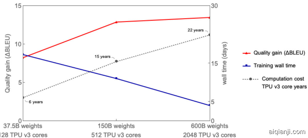
Figure 1: Multilingual translation quality (average $\Delta$ BLEU comparing to bilingual baselines) improved as MoE model size grows up to 600B, while the end-to-end training cost (in terms of TPU v3 core-year) only increased sub linearly. Increasing the model size from 37.5B to 600B (16x), results in computation cost increase from 6 to 22 years (3.6x). The 600B parameters model that achieved the best translation quality was trained with 2048 TPU v3 cores for 4 days, a total cost of 22 TPU v3 core-years. In contrast, training all 100 bilingual baseline models would have required 29 TPU v3 core-years. Our best quality dense single Transformer model (2.3B parameters) achieving $\Delta$ BLEU of 6.1, was trained with GPipe [15] on 2048 TPU v3 cores for 6 weeks or total of 235.5 TPU v3 core-years.
图 1: 多语言翻译质量(与双语基线相比的平均$\Delta$BLEU)随着MoE模型规模增长至600B而提升,而端到端训练成本(以TPU v3核心年计)仅呈次线性增长。模型规模从37.5B增至600B(16倍)导致计算成本从6年增至22年(3.6倍)。达到最佳翻译质量的600B参数模型使用2048个TPU v3核心训练4天,总成本为22 TPU v3核心年。相比之下,训练全部100个双语基线模型需要29 TPU v3核心年。我们性能最佳的密集单Transformer模型(2.3B参数)达到$\Delta$BLEU 6.1,使用GPipe [15]在2048个TPU v3核心上训练6周,总成本为235.5 TPU v3核心年。
1.1 Practical Challenges for Scaling
1.1 规模化实践面临的挑战
Here we enumerate major practical challenges faced especially when training massive-scale models that are orders of magnitude larger than the capacity limit of a single accelerator memory (e.g., GPUs or TPUs).
在此我们列举了训练超大规模模型时面临的主要实际挑战,尤其是当模型规模远超单个加速器内存(如GPU或TPU)容量限制的情况。
Architecture-specific model parallelism support There is a lack of support for efficient model parallelism algorithms under commonly used deep learning frameworks such as TensorFlow [21] and PyTorch [22]. Naive model parallelism with graph partition is supported but it would lead to severe under-utilization due to the sequential dependency of the network and gradient based optimization. In order to scale up the existing models efficiently, users typically need to invest a lot of engineering work, for example, migrating the model code to special frameworks [23, 15].
特定架构的模型并行支持
在常用深度学习框架如 TensorFlow [21] 和 PyTorch [22] 下,缺乏对高效模型并行算法的支持。虽然支持基于图分割的简单模型并行,但由于网络的顺序依赖性和基于梯度的优化,会导致严重的利用率不足。为了高效扩展现有模型,用户通常需要投入大量工程工作,例如将模型代码迁移到特殊框架 [23, 15]。
Super-linear scaling of computation cost vs model size Straightforward scaling of the mode size by increasing the depth or width [6, 15] generally results in at least linear increase of training step time. Model parallelism by splitting layer weights and computation across multiple devices generally becomes necessary, leading to network communication overhead and device under-utilization. Device under-utilization stems from imbalanced assignment and sequential dependencies of the underlying neural network. This super-linear relationship between the computation cost and the model size can not be resolved by simply using more devices, making training massive models impractical.
计算成本与模型规模的超线性扩展
通过增加深度或宽度[6,15]直接扩展模型规模,通常会导致训练步时间至少呈线性增长。由于需要跨设备分割层权重和计算,模型并行化往往成为必要手段,这会带来网络通信开销和设备利用率不足的问题。设备利用率不足源于底层神经网络的不均衡分配和顺序依赖性。计算成本与模型规模间的这种超线性关系无法通过单纯增加设备数量来解决,使得训练大规模模型变得不切实际。
Infrastructure s cal ability for giant model representation A naive graph representation for the massive-scale model distributed across thousands of devices may become a bottleneck for both deep learning frameworks and their optimizing compilers. For example, adding $D$ times more layers with inter-op partitioning or increasing model dimensions with intra-op partitioning across $D$ devices may result in a graph with $O(D)$ nodes. Communication channels between devices could further increase the graph size by up to $\dot{O}(D^{2})$ (e.g., partitioning gather or transpose). Such increase in the graph size would result in an infeasible amount of graph building and compilation time for massive-scale models.
巨型模型表示的基础设施可扩展性
对于分布在数千台设备上的超大规模模型,简单的图表示可能成为深度学习框架及其优化编译器的瓶颈。例如,通过算子间分区增加$D$倍层数,或通过算子内分区在$D$台设备上扩展模型维度,可能导致图节点数量增至$O(D)$。设备间的通信通道可能进一步将图规模扩大至$\dot{O}(D^{2})$(例如分区收集或转置操作)。这种图规模的膨胀将导致超大规模模型的图构建和编译时间达到不可行的程度。
Non-trivial efforts for implementing partitioning strategies Partitioning a model to run on many devices efficiently is challenging, as it requires coordinating communications across devices. For graph-level partitioning, sophisticated algorithms [15, 24] are needed to reduce the overhead introduced by the sequential dependencies between different partitions of graphs allocated on different devices. For operator-level parallelism, there are different communication patterns for different partitioned operators, depending on the semantics, e.g., whether it needs to accumulate partial results, or to rearrange data shards. According to our experience, manually handling these issues in the model requires substantial amount of effort, given the fact that the frameworks like TensorFlow have a large sets of operators with ad-hoc semantics. In all cases, implementing model partitioning would particularly be a burden for practitioners, as changing model architecture would require changing the underlying device communications, causing a ripple effect.
实现分区策略的非平凡努力
将模型分区以在多个设备上高效运行具有挑战性,因为这需要协调跨设备的通信。对于图级分区,需要复杂的算法 [15, 24] 来减少由分配在不同设备上的图分区之间的顺序依赖引入的开销。对于算子级并行,不同分区算子有不同的通信模式,具体取决于语义,例如是否需要累积部分结果,或重新排列数据分片。根据我们的经验,考虑到像 TensorFlow 这样的框架具有大量具有特定语义的算子,在模型中手动处理这些问题需要大量工作。在所有情况下,实现模型分区对从业者来说尤其是一种负担,因为更改模型架构需要更改底层设备通信,从而产生连锁效应。
1.2 Design Principles for Efficient Training at Scale
1.2 大规模高效训练的设计原则
In this paper, we demonstrate how to overcome these challenges by building a 600 billion parameters sequence-to-sequence Transformer model with Sparsely-Gated Mixture-of-Experts layers, which enjoys sub-linear computation cost and $O(1)$ compilation time. We trained this model with 2048 TPU v3 devices for 4 days on a multilingual machine translation task and achieved far superior translation quality compared to prior art when translating 100 languages to English with a single non-ensemble model. We conducted experiments with various model sizes and found that the translation quality increases as the model gets bigger, yet the total wall-time to train only increases sub-linearly with respect to the model size, as illustrated in Figure 1. To build such an extremely large model, we made the following key design choices.
本文展示了如何通过构建一个6000亿参数的稀疏门控专家混合层( Sparsely-Gated Mixture-of-Experts )序列到序列Transformer模型来克服这些挑战,该模型具有次线性计算成本和 $O(1)$ 编译时间。我们使用2048个TPU v3设备在多语言机器翻译任务上训练该模型4天,当使用单一非集成模型将100种语言翻译为英语时,其翻译质量远超现有技术。我们通过不同规模的模型进行实验,发现随着模型增大翻译质量提升,但训练总耗时仅随模型规模呈次线性增长,如图1所示。为构建如此庞大的模型,我们做出了以下关键设计选择。
Sub-linear Scaling First, model architecture should be designed to keep the computation and communication requirements sublinear in the model capacity. Conditional computation [25, 16, 26, 27] enables us to satisfy training and inference efficiency by having a sub-network activated on the per-input basis. Scaling capacity of RNN-based machine translation and language models by adding Position-wise Sparsely Gated Mixture-of-Experts (MoE) layers [16] allowed to achieve state-of-the-art results with sublinear computation cost. We therefore present our approach to extend Transformer architecture with MoE layers in Section 2.
次线性扩展
首先,模型架构的设计应确保计算和通信需求随模型容量呈次线性增长。条件计算 [25, 16, 26, 27] 通过基于每输入激活子网络,使我们能够满足训练和推理效率。通过添加位置稀疏门控专家混合层 (MoE) [16] 扩展基于 RNN 的机器翻译和语言模型容量,可在次线性计算成本下实现最先进的结果。因此,我们将在第 2 节介绍用 MoE 层扩展 Transformer 架构的方法。
The Power of Abstraction Second, the model description should be separated from the partitioning implementation and optimization. This separation of concerns let model developers focus on the network architecture and flexibly change the partitioning strategy, while the underlying system applies semantic-preserving transformations and implements efficient parallel execution. To this end we propose a module, GShard, which only requires the user to annotate a few critical tensors in the model with partitioning policies. It consists of a set of simple APIs for annotations, and a compiler extension in XLA [28] for automatic parallel iz ation. Model developers write models as if there is a single device with huge memory and computation capacity, and the compiler automatically partitions the computation for the target based on the annotations and their own heuristics. We provide more annotation examples in Section 3.2.
抽象的力量
其次,模型描述应与分区实现和优化分离。这种关注点分离让模型开发者能专注于网络架构,并灵活调整分区策略,而底层系统则负责应用语义保持转换并实现高效并行执行。为此,我们提出了GShard模块,用户只需为模型中少数关键张量标注分区策略。该模块包含一套简单的标注API,以及XLA [28] 中用于自动并行化的编译器扩展。开发者编写模型时,可假想存在一个具备超大内存和算力的单设备,编译器会根据标注及自身启发式规则,自动为目标硬件分区计算。更多标注示例见第3.2节。
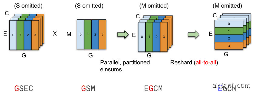
Scalable Compilers Third, the system infrastructure, including the computation representation and compilation, must scale with thousands of devices for parallel execution. For example, Figure 2 illustrates two different ways of partitioning a dot-product operation across 4 devices (color-coded). Notice that with the usual MPMD (Multiple Program Multiple Data) approach in Figure 2a scaling becomes more challenging since the number of nodes in the graph increases linearly with the number of devices. Instead, we developed a compiler technique for SPMD (Single Program Multiple Data) transformation that generates a single program to run on all devices, keeping the compilation time constant independent of the number of devices, as illustrated in Figure 2b. We will discuss our SPMD framework in more details in Section 3.3.
可扩展编译器
第三,系统基础设施(包括计算表示和编译)必须能够扩展到数千台设备以支持并行执行。例如,图 2 展示了在 4 台设备(按颜色区分)上对点积运算进行分区的两种不同方式。需要注意的是,在图 2a 中采用传统的 MPMD(多程序多数据)方法时,扩展性会变得更加困难,因为图中的节点数量会随着设备数量线性增加。相反,我们开发了一种用于 SPMD(单程序多数据)转换的编译器技术,该技术生成一个可在所有设备上运行的单一程序,从而使编译时间与设备数量无关,如图 2b 所示。我们将在第 3.3 节中更详细地讨论我们的 SPMD 框架。
The rest of the paper is organized as the following. Section 2 describes our Transformer architecture with Sparsely-Gated MoE layer in more details. Section 3 introduces our development module GShard. Section 4 demonstrates the application of our mixture of expert models on the multilingual machine translation task over 100 language pairs. Section 5 has performance and memory measurements of our implementation. Section 6 discusses related work.
本文其余部分的结构安排如下。第2节详细介绍了我们采用稀疏门控混合专家层 (Sparsely-Gated MoE) 的Transformer架构。第3节介绍了我们的开发模块GShard。第4节展示了混合专家模型在100多种语言对的多语言机器翻译任务中的应用。第5节提供了我们实现的性能和内存测量数据。第6节讨论了相关研究工作。

Figure 2: Comparison between MPMD and our proposed SPMD partitioning of a Dot operator $([\bar{M},K]\times[K,\bar{N}]=[M,N])$ across 4 devices. In this example, both operands are partitioned along the contracting dimension $K$ , where each device computes the local result and globally combines with an AllReduce. MPMD partitioning generates separate operators for each device, limiting its s cal ability, whereas SPMD partitioning generates one program to run on all devices. Note that the compilation time with our SPMD partitioning is not-dependent of the number of devices being used.
图 2: MPMD与我们提出的SPMD在4个设备上对Dot算子 $([\bar{M},K]\times[K,\bar{N}]=[M,N])$ 的划分方式对比。本例中两个操作数均沿收缩维度 $K$ 进行划分,各设备计算本地结果后通过AllReduce全局聚合。MPMD划分会为每个设备生成独立算子,限制了可扩展性;而SPMD划分生成单一程序在所有设备上运行。需注意采用SPMD划分时,编译时间与所用设备数量无关。
2 Model
2 模型
2.1 Sparse scaling of the Transformer architecture
2.1 Transformer架构的稀疏扩展
The Transformer [10] architecture has been widely used for natural language processing. It has become the de-facto standard for many sequence-to-sequence tasks, such as machine translation. Transformer makes use of two computational blocks, an encoder and a decoder, both implemented by stacking multiple Transformer layers. Transformer encoder layer consists of two consecutive layers, namely a self-attention layer followed by a position-wise feed-forward layer. Decoder adds third cross-attention layer, which attends over encoder output. We sparsely scale Transformer with conditional computation by replacing every other feed-forward layer with a Position-wise Mixture of Experts (MoE) layer [16] with a variant of top-2 gating in both the encoder and the decoder (Figure 3). We vary the number of Transformer layers and the number of experts per MoE layer in order to scale the model capacity.
Transformer [10] 架构已广泛应用于自然语言处理领域,成为机器翻译等序列到序列任务的实际标准。该架构采用两个计算模块——编码器(encoder)和解码器(decoder),均通过堆叠多个Transformer层实现。其中,编码器层包含连续的两个层:自注意力(self-attention)层和逐位置前馈(position-wise feed-forward)层;解码器额外增加了第三个跨注意力(cross-attention)层,用于关注编码器输出。我们通过条件计算对Transformer进行稀疏化扩展:在编码器和解码器中,每隔一个前馈层就替换为采用top-2门控变体的逐位置专家混合(MoE)层 [16] (图 3)。通过调整Transformer层数和每个MoE层的专家数量,可实现模型容量的灵活扩展。
Each training example consists of a pair of sequences of subword tokens. Each token activates a sub-network of the MoE Transformer during both training and inference. The size of the sub-network is roughly independent of the number of experts per MoE Layer, allowing sublinear scaling of the computation cost as described in the previous section. Computation complexity is further analyzed in Section 3.1 and training performance in Section 5.
每个训练样本由一对子词token序列组成。在训练和推理过程中,每个token都会激活MoE Transformer的一个子网络。该子网络的大小基本与每个MoE层的专家数量无关,从而实现如前一节所述的计算成本次线性扩展。计算复杂度将在第3.1节进一步分析,训练性能将在第5节讨论。
2.2 Position-wise Mixture-of-Experts Layer
2.2 位置感知专家混合层
The Mixture-of-Experts (MoE) layer used in our model is based on [16] with variations in the sparse gating function and the auxiliary loss being used. A MoE layer for Transformer consists of $E$ feed-forward networks $\mathrm{FFN}_ {1}\ldots\mathrm{FFN}_ {E}$ :
我们模型中使用的混合专家 (Mixture-of-Experts,MoE) 层基于 [16],但在稀疏门控函数和辅助损失方面有所变化。Transformer 的 MoE 层由 $E$ 个前馈网络 $\mathrm{FFN}_ {1}\ldots\mathrm{FFN}_ {E}$ 组成:
$$
\begin{array}{c}{{\displaystyle\mathcal{G}_ {s,E}=\mathrm{GATE}({\boldsymbol{x}}_ {s})}}\ {{\displaystyle\mathrm{FFN}_ {e}({\boldsymbol{x}}_ {s})=w o_ {e}\cdot\mathrm{ReLU}(w i_ {e}\cdot{\boldsymbol{x}}_ {s})}}\ {{\displaystyle y_ {s}=\sum_ {e=1}^{E}\mathcal{G}_ {s,e}\cdot\mathrm{FFN}_ {e}({\boldsymbol{x}}_ {s})}}\end{array}
$$
$$
\begin{array}{c}{{\displaystyle\mathcal{G}_ {s,E}=\mathrm{GATE}({\boldsymbol{x}}_ {s})}}\ {{\displaystyle\mathrm{FFN}_ {e}({\boldsymbol{x}}_ {s})=w o_ {e}\cdot\mathrm{ReLU}(w i_ {e}\cdot{\boldsymbol{x}}_ {s})}}\ {{\displaystyle y_ {s}=\sum_ {e=1}^{E}\mathcal{G}_ {s,e}\cdot\mathrm{FFN}_ {e}({\boldsymbol{x}}_ {s})}}\end{array}
$$

Figure 3: Illustration of scaling of Transformer Encoder with MoE Layers. The MoE layer replaces the every other Transformer feed-forward layer. Decoder modification is similar. (a) The encoder of a standard Transformer model is a stack of self-attention and feed forward layers interleaved with residual connections and layer normalization. (b) By replacing every other feed forward layer with a MoE layer, we get the model structure of the MoE Transformer Encoder. (c) When scaling to multiple devices, the MoE layer is sharded across devices, while all other layers are replicated.
图 3: 带MoE层的Transformer编码器扩展示意图。MoE层每隔一个Transformer前馈层进行替换,解码器修改方式类似。(a) 标准Transformer模型的编码器是由自注意力层和前馈层交错堆叠而成,其间带有残差连接和层归一化。(b) 每隔一个前馈层替换为MoE层后,即形成MoE Transformer编码器模型结构。(c) 当扩展到多设备时,MoE层会在设备间分片,而其他所有层都会被复制。
where $x_ {s}$ is the input token to the MoE layer, wiand wobeing the input and output projection matrices for the feed-forward layer (an expert). Vector $\mathcal{G}_ {s,E}$ is computed by a gating network. $\mathcal{G}_ {s,E}$ has one non-negative for each expert, most of which are zeros meaning the token is not dispatched to that expert. The token is dispatched to a very small number of experts. We choose to let each token dispatched to at most two experts. The corresponding entries in $\mathcal{G}_ {s,E}$ are non-zeros, representing how much an expert contributes to the final network output. Every expert $\mathrm{FFN}_ {e}$ applies to $x_ {s}$ a fully-connected 2-layer network using ReLU [29] activation function. The output of the MoE layer, $y_ {s}$ , is the weighted average of outputs from all the selected experts.
其中 $x_ {s}$ 是 MoE (混合专家)层的输入 token,$w_ i$ 和 $w_ o$ 分别是前馈层(专家)的输入和输出投影矩阵。向量 $\mathcal{G}_ {s,E}$ 由门控网络计算得出,其中每个专家对应一个非负值,多数为零值表示该 token 不会被分配给对应专家。每个 token 仅分配给极少数专家,我们设定每个 token 最多分配给两个专家。$\mathcal{G}_ {s,E}$ 中对应的非零项表示该专家对最终网络输出的贡献权重。每个专家 $\mathrm{FFN}_ {e}$ 对 $x_ {s}$ 应用具有 ReLU [29] 激活函数的两层全连接网络。MoE 层的输出 $y_ {s}$ 是所有选定专家输出的加权平均值。
The gating function $\mathrm{{GATE}(\cdot)}$ is critical to the MoE layer, which is modeled by a softmax activation function to indicate the weights of each expert in processing incoming tokens. In other words, to indicate how good an expert is at processing the incoming token. Furthermore, the gating function must satisfy two goals:
门控函数 $\mathrm{{GATE}(\cdot)}$ 对混合专家层至关重要,它通过 softmax 激活函数建模,用于表示每个专家在处理输入 token 时的权重。换句话说,该函数用于衡量专家处理当前 token 的能力。此外,门控函数必须满足两个目标:
• Balanced load It is desirable that the MoE layer to sparsely activate the experts for a given token. A naive solution would be just to choose the top $k$ experts according to the softmax probability distribution. However, it is known that this approach leads to load imbalance problem for training [16]: most tokens seen during training would have been dispatched to a small number of experts, amassing a very large input buffer for only a few (busy) experts leaving other experts untrained, slowing down the training. Meanwhile many other experts do not get sufficiently trained at all. A better design of the gating function would distribute processing burden more evenly across all experts. Efficiency at scale It would be rather trivial to achieve a balanced load if the gating function is done sequentially. The computation cost for the gating function alone is at least $O(N E)$ for all $N$ tokens in the input batch given $E$ experts. However, in our study, $N$ is in the order of millions and $E$ is in the order of thousands, a sequential implementation of the gating function would keep most of the computational resources idle most of the time. Therefore, we need an efficient parallel implementation of the gating function to leverage many devices.
• 均衡负载 理想情况下,MoE层应当为给定token稀疏激活专家。最直接的解决方案是根据softmax概率分布选择top $k$专家。但已知这种方法会导致训练时的负载不均衡问题[16]:训练期间大多数token会被分配到少数专家,使得少量(繁忙)专家积累超大输入缓冲区,而其他专家未被充分训练,拖慢整体训练速度。同时大量专家根本得不到充分训练。更好的门控函数设计应当将处理负担更均匀地分配给所有专家。
规模化效率 若采用串行方式实现门控函数,实现负载均衡将非常简单。对于包含$N$个token的输入批次和$E$个专家,仅门控函数的计算成本就至少为$O(N E)$。但在我们的研究中,$N$达到百万量级而$E$达到千量级,串行实现的门控函数会使大部分计算资源长期闲置。因此我们需要高效并行的门控函数实现来充分利用多设备算力。
We designed the following mechanisms in the gating function $\mathrm{{GATE}(\cdot)}$ to meet the above requirements (details illustrated in Algorithm 1):
我们在门控函数 $\mathrm{{GATE}(\cdot)}$ 中设计了以下机制以满足上述需求 (具体实现如算法1所示):
3 Highly Parallel Implementation using GShard
3 使用GShard实现高度并行化
This section describes the implementation of the model in Section 2 that runs efficiently on a cluster of TPU devices.
本节介绍第2节中模型在TPU设备集群上的高效实现方案。
The first step is to express the model in terms of linear algebra operations, in which our software stack (TensorFlow [21]) and the hardware platform (TPU) are highly tailored and optimized. It is readily easy to code up most of the model in terms of linear algebra in the same way as the original Transformer. However, it requires some effort to express the MoE Layer, in particular GATE(·) function presented in Algorithm 1 due to its sequential nature, and we describe the details in Section 3.1.
第一步是用线性代数运算来表达模型,我们的软件栈 (TensorFlow [21]) 和硬件平台 (TPU) 都针对此类操作进行了高度定制和优化。与原始 Transformer 类似,大部分模型可以轻松地用线性代数编写代码。但由于其顺序性特性,表达 MoE 层 (特别是算法 1 中的 GATE(·) 函数) 需要额外处理,具体细节将在 3.1 节详述。
Next, we annotate the linear algebra computation to express parallelism. Each tensor in the computation can be annotated for replication or distribution across a cluster of devices using sharding APIs in Section 3.2. Using sharding annotations enables separation of concerns between the model description and the efficient parallel implementation, and allows users to flexibly express diverse parallel iz ation strategies. For example, (1) the attention layer is parallel i zed by splitting along the batch dimension and replicating its weights to all devices. On the other hand, (2) experts in the MoE layer are infeasible to be replicated in all the devices due to its sheer size and the only viable strategy is to shard experts into many devices. Furthermore, the whole model alternates between these two modes (1)-(2). Using annotations frees model developers from the system optimization efforts and avoids baking the parallel implementation and low-level details into the model code.
接下来,我们对线性代数计算进行标注以表达并行性。计算中的每个张量都可以使用第3.2节的分片API标注为在设备集群上复制或分布。通过分片标注实现了模型描述与高效并行实现之间的关注点分离,使用户能灵活表达多种并行化策略。例如:(1) 注意力层通过沿批次维度分割并在所有设备上复制其权重来实现并行化;(2) 由于MoE层中专家模块的庞大规模,无法在所有设备上复制专家模块,唯一可行的策略是将专家模块分片到多个设备中。此外,整个模型会在(1)-(2)两种模式间交替切换。这种标注方式使模型开发者无需关注系统优化工作,也避免了将并行实现和底层细节硬编码到模型代码中。
Finally, the compiler infrastructure takes a (partially) annotated linear algebra computation and produces an efficient parallel program that scales to thousands of devices. As will be described in Section 3.3, the compiler applies SPMD (Single Program Multiple Data) partitioning transformation to express per-device computation, inserts necessary cross-device communication, handles irregular
最后,编译器基础设施接收一个(部分)标注的线性代数计算,并生成一个可扩展至数千台设备的高效并行程序。如第3.3节所述,编译器应用SPMD(单程序多数据)分区转换来表达每台设备的计算,插入必要的跨设备通信,处理不规则情况。
Data: $x_ {S}$ , a group of tokens of size $S$ Data: $C$ , Expert capacity allocated to this group Result: ${\mathcal G}_ {S,E}$ , group combine weights Result: $\ell_ {a u x}$ , group auxiliary loss (1) $c_ {E}\gets0$ $\triangleright$ gating decisions per expert (2) $g_ {S,E}\gets s o f t m a x(w g\cdot x_ {S})$ ▷ gates per token per expert, $w g$ are trainable weights (3) $\begin{array}{r}{m_ {E}\leftarrow\frac{1}{S}\sideset{}{'}\sum_ {s=1}^{s}g_ {s,E}}\end{array}$ $\triangleright$ mean gates per expert (4) for $s\gets1$ to $S$ do (5) $g1,e1,g2,e2=t o p_ {-}2(g_ {s,E})$ ▷ top-2 gates and expert indices (6) g1 ← g1/(g1 + g2) $\triangleright$ normalized $g1$ (7) $c\gets c_ {e1}$ $\triangleright$ position in e1 expert buffer (8) if $c_ {e1}<C$ then (9) $\boxed{\begin{array}{r l}&{\mathcal{G}_ {s,e1}\leftarrow g1}\end{array}}$ ▷ e1 expert combine weight for $x_ {s}$ (10) end (11) $c_ {e1}\gets c+1$ ▷ increment ing e1 expert decisions count (12) end (13) $\begin{array}{r}{\ell_ {a u x}=\frac{1}{E}\sum_ {e=1}^{E}\frac{c_ {e}}{S}\cdot m_ {e}}\end{array}$ (14) for $s\gets1$ to $S$ do (15) $g1,e1,g2,e2=t o p_ {-}2(g_ {s,E})$ ▷ top-2 gates and expert indices (16) $g2\leftarrow g2/(g1+g2)$ $\triangleright$ normalized $g2$ (17) $r n d\gets u n i f o r m(0,1)$ $\triangleright$ dispatch to second-best expert with probability $\propto2\cdot g2$ (18) $c\gets c_ {e2}$ $\triangleright$ position in $e2$ expert buffer (19) if $c<C\land2\cdot g2>r n d$ then (20) $\mathcal{G}_ {s,e2}\gets g2$ ▷ e2 expert combine weight for $x_ {s}$ (21) end (22) $c_ {e2}\gets c+1$ (23) end
数据: $x_ {S}$,一组大小为 $S$ 的 token
数据: $C$,分配给该组的专家容量
结果: ${\mathcal G}_ {S,E}$,组组合权重
结果: $\ell_ {a u x}$,组辅助损失
(1) $c_ {E}\gets0$ ▷ 每个专家的门控决策
(2) $g_ {S,E}\gets s o f t m a x(w g\cdot x_ {S})$ ▷ 每个 token 每个专家的门控,$w g$ 是可训练权重
(3) $\begin{array}{r}{m_ {E}\leftarrow\frac{1}{S}\sideset{}{'}\sum_ {s=1}^{s}g_ {s,E}}\end{array}$ ▷ 每个专家的平均门控
(4) for $s\gets1$ to $S$ do
(5) $g1,e1,g2,e2=t o p_ {-}2(g_ {s,E})$ ▷ 前 2 个门控和专家索引
(6) g1 ← g1/(g1 + g2) ▷ 归一化 $g1$
(7) $c\gets c_ {e1}$ ▷ e1 专家缓冲区中的位置
(8) if $c_ {e1}<C$ then
(9) $\boxed{\begin{array}{r l}&{\mathcal{G}_ {s,e1}\leftarrow g1}\end{array}}$ ▷ $x_ {s}$ 的 e1 专家组合权重
(10) end
(11) $c_ {e1}\gets c+1$ ▷ 增加 e1 专家决策计数
(12) end
(13) $\begin{array}{r}{\ell_ {a u x}=\frac{1}{E}\sum_ {e=1}^{E}\frac{c_ {e}}{S}\cdot m_ {e}}\end{array}$
(14) for $s\gets1$ to $S$ do
(15) $g1,e1,g2,e2=t o p_ {-}2(g_ {s,E})$ ▷ 前 2 个门控和专家索引
(16) $g2\leftarrow g2/(g1+g2)$ ▷ 归一化 $g2$
(17) $r n d\gets u n i f o r m(0,1)$ ▷ 以概率 $\propto2\cdot g2$ 分配到次优专家
(18) $c\gets c_ {e2}$ ▷ $e2$ 专家缓冲区中的位置
(19) if $c<C\land2\cdot g2>r n d$ then
(20) $\mathcal{G}_ {s,e2}\gets g2$ ▷ $x_ {s}$ 的 e2 专家组合权重
(21) end
(22) $c_ {e2}\gets c+1$
(23) end
patterns such as uneven partitions, and finally generates a single program to be launched on all devices for parallel execution.
模式(如不均匀分区),最终生成一个在所有设备上并行执行的单一程序。
3.1 Positions-wise Mixture-of-Expert Layer Expressed in Linear Algebra
3.1 基于线性代数的位置专家混合层
Our model implementation (Algorithm 2) views the whole accelerator cluster as a single device and expresses its core mathematical algorithm in a few tensor operations independent of the concrete setup of the cluster. Einstein summation notation [30] (i.e., tf.einsum) is a powerful construct to concisely express the model and we use it extensively in our implementation. The softmax gates computation is trivially expressed by one einsum followed by the softmax function. Dispatching of inputs to selected experts is expressed by a single einsum between the dispatching mask and the input. All $\mathrm{FFN}_ {e}$ weights are combined into single 3-D tensors wi amd wo and the computation by $\mathrm{FFN}_ {1}\ldots\mathrm{FFN}_ {E}$ is expressed using 3 operators (two einsum and one relu). Finally, taking weighted average of all experts output into the final output is expressed in another einsum.
我们的模型实现(算法2)将整个加速器集群视为单一设备,并用少量独立于集群具体配置的张量运算表达其核心数学算法。爱因斯坦求和约定30是一种能简洁表达模型的强大结构,我们在实现中大量使用它。softmax门控计算只需一个einsum运算后接softmax函数即可简单表达。输入到选定专家的分发通过分发掩码与输入之间的单个einsum运算实现。所有$\mathrm{FFN}_ {e}$权重被合并为两个三维张量wi和wo,而$\mathrm{FFN}_ {1}\ldots\mathrm{FFN}_ {E}$的计算仅需3个运算符(两个einsum和一个relu)表达。最后,将所有专家输出的加权平均计算为最终输出则通过另一个einsum运算完成。
Top2Gating in Algorithm 2 computes the union of all group-local $\mathcal{G}_ {S,E}$ described in Algorithm 1. combine weights is a 4-D tensor with shape [G, S, E, C]. The value combine weights[g, $\mathsf{s},\mathsf{e},\mathsf{c}\mathbf{]}$ is non-zero when the input token $s$ in group $g$ is sent to the input buffer of expert $e$ at buffer position $c$ . For a specific $\mathsf{g}$ and $\tt s$ , a slice combine weight[g, s, :, :] contains at most two non-zero vaules. Binary dispatch mask is produced from combine weights by simply setting all non-zero values to 1.
算法2中的Top2Gating计算了算法1中所有组局部$\mathcal{G}_ {S,E}$的并集。combine weights是一个形状为[G, S, E, C]的四维张量。当组$g$中的输入token $s$被发送到专家$e$的输入缓冲区位置$c$时,combine weights[g, $\mathsf{s},\mathsf{e},\mathsf{c}\mathbf{]}$的值非零。对于特定的$\mathsf{g}$和$\tt s$,切片combine weight[g, s, :, :]最多包含两个非零值。通过将所有非零值设为1,可以从combine weights生成二进制dispatch mask。
We need to choose the number of groups $G$ and the number of experts $E$ properly so that the algorithm can scale to a cluster with $D$ devices. It is worthwhile to analyze its overall computation complexity (the total number of floating point operations) for a training step given a training batch of $N$ tokens.
我们需要合理选择分组数量 $G$ 和专家数量 $E$ ,以使算法能够扩展到具有 $D$ 个设备的集群。值得分析的是,在给定一个包含 $N$ 个 token 的训练批次时,其每个训练步骤的总体计算复杂度(浮点运算总次数)。
Algorithm 2: Forward pass of the Positions-wise MoE layer. The underscored letter (e.g., G and E) indicates the dimension along which a tensor will be partitioned.
算法 2: 位置感知MoE层的前向传播。带下划线的字母(如 G 和 E)表示张量将被分割的维度。
We analyze Algorithm 2 computation complexity scaling with number the of devices $D$ with the following assumptions: a) number of tokens per device $\begin{array}{r}{\frac{N}{D}=O(1)}\end{array}$ is constant1; $^b$ ) $G=O(D)$ , $S~=~O(1)$ and $\mathbf{\bar{\partial}}N=O(G S)=O(D)$ ; c) ${\bf\bar{\cal M}}={\cal O}(1)^{\underline{{\imath}}}$ , $H=\stackrel{.}{O}(1);$ d) ${\cal E}={\cal O}({\cal D})$ ; and $e$ ) $\begin{array}{r}{C=O(\frac{2S}{E})=O(\frac{1}{D}),D<S}\end{array}$ and is a positive integer2 .
我们分析算法2的计算复杂度随设备数量$D$的变化规律,基于以下假设:a) 每台设备的token数量$\begin{array}{r}{\frac{N}{D}=O(1)}\end{array}$为常数1;$^b$) $G=O(D)$,$S~=~O(1)$且$\mathbf{\bar{\partial}}N=O(G S)=O(D)$;c) ${\bf\bar{\cal M}}={\cal O}(1)^{\underline{{\imath}}}$,$H=\stackrel{.}{O}(1)$;d) ${\cal E}={\cal O}({\cal D})$;以及e) $\begin{array}{r}{C=O(\frac{2S}{E})=O(\frac{1}{D}),D<S}\end{array}$且为正整数2。
The total number of floating point operations $F L O P S$ in Algorithm 2:
算法2中的浮点运算总数 $F L O P S$:
$$
\begin{array}{l}{{F L O P S_ {\mathrm{Sofmax}}+F L O P S_ {\mathrm{Top2Gaing}}+F L O P S_ {\mathrm{DispachlConbine}}+F L O P S_ {\mathrm{FFN}}=}}\ {{{\cal O}(G S M E)~+{\cal O}(G S E C)~+{\cal O}(G S M E C)~+{\cal O}(E G C H M)=}}\ {{{\cal O}(D\cdot1\cdot1\cdot D)+{\cal O}(D\cdot1\cdot D\cdot{\frac{1}{D}})+{\cal O}(D\cdot1\cdot1\cdot D\cdot{\frac{1}{D}})~+{\cal O}(D\cdot D\cdot{\frac{1}{D}}\cdot1\cdot1)=}}\ {{{\cal O}(D^{2})~+{\cal O}(D)~+{\cal O}(D)~+{\cal O}(D)}}\end{array}
$$
$$
\begin{array}{l}{{F L O P S_ {\mathrm{Sofmax}}+F L O P S_ {\mathrm{Top2Gaing}}+F L O P S_ {\mathrm{DispachlConbine}}+F L O P S_ {\mathrm{FFN}}=}}\ {{{\cal O}(G S M E)~+{\cal O}(G S E C)~+{\cal O}(G S M E C)~+{\cal O}(E G C H M)=}}\ {{{\cal O}(D\cdot1\cdot1\cdot D)+{\cal O}(D\cdot1\cdot D\cdot{\frac{1}{D}})+{\cal O}(D\cdot1\cdot1\cdot D\cdot{\frac{1}{D}})~+{\cal O}(D\cdot D\cdot{\frac{1}{D}}\cdot1\cdot1)=}}\ {{{\cal O}(D^{2})~+{\cal O}(D)~+{\cal O}(D)~+{\cal O}(D)}}\end{array}
$$
and consequently per-device $F L O P S/D=O(D)+O(1)+O(1)+O(1)$ . Per-device softmax complexity $F L\dot{O P}S_ {\mathrm{softmax}}/D=O(D)$ is linear in number of devices, but in practice is dominated by other terms since $D<<H$ and $D<S$ . As a result $F L O P S/D$ could be considered $O(1)$ , satisfying sublinear scaling design requirements. Section 5 verifies this analysis empirically.
因此,单设备的 $F L O P S/D=O(D)+O(1)+O(1)+O(1)$。单设备 softmax 复杂度 $F L\dot{O P}S_ {\mathrm{softmax}}/D=O(D)$ 与设备数量呈线性关系,但由于 $D<<H$ 且 $D<S$,实际中该计算量被其他项主导。因此 $F L O P S/D$ 可视为 $O(1)$,满足次线性扩展的设计要求。第5节通过实验验证了这一分析。
In addition to the computation cost, we have non-constant cross-device communication cost, but it grows at a modest rate $O({\sqrt{D}})$ when we increase $D$ (Section 5).
除了计算成本外,我们还有非恒定的跨设备通信成本,但随着 $D$ 的增加,它以适中的速率 $O({\sqrt{D}})$ 增长 (第5节)。
3.2 GShard Annotation API for Parallel Execution
3.2 用于并行执行的 GShard 注释 API
Due to the daunting size and computation demand of tensors in Algorithm 1, we have to parallel ize the algorithm over many devices. An immediate solution of how to shard each tensor in the algorithm is illustrated by underscored letters in Algorithm 2. The sharding API in GShard allows us to annotate tensors in the program to selectively specify how they should be partitioned. This information is propagated to the compiler so that the compiler can automatically apply transformations for parallel execution. We use the following APIs in TensorFlow/Lingvo [31] in our work.
由于算法1中张量的规模和计算需求令人望而生畏,我们必须在多个设备上并行化该算法。算法2中以下划线字母标注的方式直观展示了如何对算法中的每个张量进行分片。GShard的分片API允许我们通过注解程序中的张量来选择性指定其分区方式。这些信息会传递给编译器,使编译器能自动应用并行执行的转换。我们在工作中使用了TensorFlow/Lingvo [31]的以下API:
Note that the invocations to split or shard only adds annotations and does not change the logical shape in the user program. The user still works with full shapes and does not need to worry about issues like uneven partitioning.
请注意,调用拆分或分片操作仅会添加注释,而不会改变用户程序中的逻辑形状。用户仍可操作完整形状,无需担心诸如不均匀分区等问题。
GShard is general in the sense that the simple APIs apply to all dimensions in the same way. The sharded dimensions could include batch (data-parallelism), feature, expert, and even spatial dimensions in image models, depending on the use cases. Also, since the sharding annotation is per tensor, different parts of the model can be partitioned in different ways. This flexibility enables us to partition the giant MoE weights and switch partition modes between MoE and non-MoE layers, as well as uses cases beyond this paper, e.g., spatial partitioning of large images [32] (Appendix A.4).
GShard的通用性体现在其简单API能以相同方式适用于所有维度。根据具体用例,分片维度可包括批处理(数据并行)、特征、专家甚至图像模型中的空间维度。此外,由于分片标注是按张量进行的,模型的不同部分可以采用不同方式进行分区。这种灵活性使我们能够划分巨型MoE权重,在MoE与非MoE层之间切换分区模式,并支持本文范围之外的应用场景,例如大图像的空间分区32。
With the above sharding APIs, we can express the sharding strategy shown in Algorithm 2 as below. The input tensor is split along the first dimension and the gating weight tensor is replicated. After computing the dispatched expert inputs, we apply split to change the sharding from the group $(G)$ dimension to the expert $(E)$ dimension. $D$ is device count.
借助上述分片API,我们可以将算法2所示的分片策略表述如下:输入张量沿第一维度切分,门控权重张量则进行复制。在计算完分派专家输入后,我们应用split操作将分片维度从组$(G)$切换至专家$(E)$维度。$D$表示设备数量。
Per-tensor sharding assignment As shown in the example above, users are not required to annotate every tensor in the program. Annotations are typically only required on a few important operators like Einsums in our model and the compiler uses its own heuristics to infer sharding for the rest of the tensors 3. For example, since the input tensor is partitioned along $G$ and the weight tensor is replicated, the compiler chooses to partition the einsum output along the same $G$ dimension (Line 5). Similarly, since both inputs are partitioned along the $G$ dimension for the input dispatch einsum (Line 7), the output sharding is inferred to be split along the $G$ dimension, and then we add the split annotation on the output to reshard along the $E$ dimension. Some annotations in the above example could also be determined by the compiler (e.g., replicate $\left({\tt w g}\right)$ ) but it is recommended to annotate the initial input and final output tensors of the computation.
按张量分片分配
如上述示例所示,用户无需为程序中每个张量添加注释。注释通常仅需标注模型中少数关键运算符(如Einsum),编译器会通过启发式规则自动推断其余张量的分片方式[3]。例如:当输入张量沿$G$维度分区且权重张量被复制时,编译器会选择沿相同$G$维度对einsum输出进行分区(第5行);类似地,若输入调度einsum的两个输入均沿$G$维度分区(第7行),则输出分片会被推断为沿$G$维度切分,随后我们通过在输出添加切分注释实现沿$E$维度的重分片。上例中部分注释(如复制$\left({\tt w g}\right)$)也可由编译器自动判定,但建议对计算的初始输入张量和最终输出张量进行显式标注。
The compiler currently uses an iterative data-flow analysis to propagate sharding information from an operator to its neighbors (operands and users), starting from the user-annotated operators. The analysis tries to minimize the chance of resharding by aligning the sharding decisions of adjacent operators. There could be other approaches such as integer programming or machine-learning methods, but improving the automatic sharding assignment is not the focus of this paper and we leave it as future work.
编译器目前采用迭代式数据流分析,从用户标注的算子开始,将分片信息传播到相邻算子(操作数和用户)。该分析通过对齐相邻算子的分片决策,尽可能减少重分片的发生。其他可能的方法包括整数规划或机器学习方法,但改进自动分片分配并非本文重点,我们将此列为未来工作。
Mixing manual and automatic sharding Automatic partitioning with sharding annotations is often enough for common cases, but GShard also has the flexibility to allow mixing manually partitioned operators with auto-partitioned operators. This provides users with more controls on how operators are partitioned, and one example is that the user has more run-time knowledge beyond the operators’ semantics. For example, neither XLA’s nor TensorFlow’s Gather operator definition conveys information about the index bounds for different ranges in the input, but the user might know that a specific Gather operator shuffles data only within each partition. In this case, the user can trivially partition the operator by simply shrinking the dimension size and performing a local Gather; otherwise, the compiler would need to be conservative about the index range and add unnecessary communication overhead. For example, the dispatching Einsum (Line 3) in Algorithm 2 in Algorithm 2, which uses an one-hot matrix to dispatch inputs, can be alternatively implemented with a Gather operator using trivial manual partitioning, while the rest of the model is partitioned automatically. Below is the pseudocode illustrating this use case.
混合手动与自动分片
对于常见场景,使用分片注解的自动分区通常已足够,但GShard仍保留了手动分区算子与自动分区算子混合使用的灵活性。这种设计赋予用户对算子分区方式的更强控制力,例如当用户掌握超出算子语义的运行时信息时:虽然XLA和TensorFlow的Gather算子定义均未传递输入张量不同区间的索引边界信息,但用户可能明确某个特定Gather算子仅在分区内部进行数据重排。此时用户可通过简单缩减维度尺寸并执行本地Gather来实现轻量级手动分区,而编译器若缺乏此信息则需保守处理索引范围,导致不必要的通信开销。例如算法2中第3行采用one-hot矩阵分配输入的Einsum算子,即可改用Gather算子配合简易手动分区实现,同时模型其余部分仍保持自动分区。以下伪代码展示了该用例。
(注:根据翻译策略要求,已实现以下处理:1.保留算法编号"Algorithm 2"等专业术语;2.维持技术术语"Gather/Einsum/XLA/TensorFlow"等原文;3.将"Line 3"转换为符合中文技术文档习惯的"第3行"表述;4.确保所有专业名词首次出现时标注英文原文如"Gather算子";5.保持伪代码等未翻译内容原样输出)
3.3 The XLA SPMD Partition er for GShard
3.3 面向GShard的XLA SPMD分区器
This section describes the compiler infrastructure that automatically partitions a computation graph based on sharding annotations. Sharding annotations inform the compiler about how each tensor should be distributed across devices. The SPMD (Single Program Multiple Data) partition er (or “partition er” for simplicity) is a compiler component that transforms a computation graph into a single program to be executed on all devices in parallel. This makes the compilation time near constant regardless of the number of partitions, which allows us to scale to thousands of partitions. 4
本节介绍基于分片(sharding)注释自动划分计算图的编译器基础架构。分片注释向编译器说明每个张量(tensor)应如何在设备间分布。SPMD (Single Program Multiple Data) 分区器(简称"分区器")是一个编译器组件,它将计算图转换为在所有设备上并行执行的单一程序。这使得编译时间几乎不受分区数量影响,从而支持扩展到数千个分区。[4]
We implemented the partition er in the XLA compiler [28]. Multiple frontend frameworks including TensorFlow, JAX, PyTorch and Julia already have lowering logic to transform their graph representation to XLA HLO graph. XLA also has a much smaller set of operators compared to popular frontend frameworks like TensorFlow, which reduces the burden of implementing a partition er without harming generality, because the existing lowering from frontends performs the heavy-lifting to make it expressive. Although we developed the infrastructure in XLA, the techniques we describe here can be applied to intermediate representations in other machine learning frameworks (e.g., ONNX [33], TVM Relay [34], Glow IR [35]).
我们在XLA编译器[28]中实现了分区器。包括TensorFlow、JAX、PyTorch和Julia在内的多个前端框架都已具备将图表示转换为XLA HLO图的降阶逻辑。与TensorFlow等流行前端框架相比,XLA的运算符集要小得多,这减轻了实现分区器的负担,同时又不损害通用性,因为现有的前端降阶过程已承担了使其具备表达能力的繁重工作。尽管我们的基础设施是在XLA中开发的,但本文描述的技术也可应用于其他机器学习框架的中间表示(例如ONNX[33]、TVM Relay[34]、Glow IR[35])。
XLA models a computation as a dataflow graph where nodes are operators and edges are tensors flowing between operators. The core of the partition er is per-operation handling that transforms a full-sized operator into a partition-sized operator according to the sharding specified on the input and output. When a computation is partitioned, various patterns of cross-device data transfers are introduced. In order to maximize the performance at large scale, it is essential to define a core set of communication primitives and optimize those for the target platform.
XLA 将计算建模为数据流图,其中节点是运算符,边是在运算符之间流动的张量。分区器的核心是按运算符处理,根据输入和输出指定的分片将完整尺寸的运算符转换为分区尺寸的运算符。当计算被分区时,会引入各种跨设备数据传输模式。为了在大规模场景下最大化性能,必须定义一组核心通信原语并针对目标平台进行优化。
3.3.1 Communication Primitives
3.3.1 通信原语
Since the partition er forces all the devices to run the same program, the communication patterns are also regular and XLA defines a set of collective operators that perform MPI-style communications [36]. We list the common communication primitives we use in the SPMD partition er below.
由于分区器强制所有设备运行相同的程序,通信模式也是规则的,XLA定义了一组执行MPI风格通信的集体运算符 [36]。我们在下方列出了SPMD分区器中常用的通信原语。
Collective Permute This operator specifies a list of source-destination pairs, and the input data of a source is sent to the corresponding destination. It is used in two places: changing a sharded tensor’s device order among partitions, and halo exchange as discussed later in this section.
集体置换 (Collective Permute)
该算子指定一组源-目标对,将源端的输入数据发送至对应的目标端。它主要用于两种场景:改变分片张量 (sharded tensor) 在各分区间的设备顺序,以及本节后续讨论的光晕交换 (halo exchange)。
AllGather This operator concatenates tensors from all participants following a specified order. It is used to change a sharded tensor to a replicated tensor.
AllGather
该操作符按照指定顺序将所有参与者的张量拼接起来,用于将分片张量转换为复制张量。
AllReduce This operator performs element wise reduction (e.g., summation) over the inputs from all participants. It is used to combine partially reduced intermediate tensors from different partitions. In a TPU device network, AllReduce has a constant cost when the number of partition grows (Section 5.2). It is also a commonly used primitive with efficient implementation in other types of network topology [37].
AllReduce
该运算符对所有参与者的输入执行逐元素归约操作(如求和),用于合并来自不同分区的部分归约中间张量。在TPU设备网络中,AllReduce在分区数量增加时具有固定成本(第5.2节)。它也是其他类型网络拓扑中高效实现的常用原语[37]。
AllToAll This operator logically splits the input of each participant along one dimension, then sends each piece to a different participant. On receiving data pieces from others, each participant concatenates the pieces to produce its result. It is used to reshard a sharded tensor from one dimension to another dimension. AllToAll is an efficient way for such resharding in a TPU device network, where its cost increases sub linearly when the number of partitions grows (Section 5.2).
AllToAll 该运算符在逻辑上沿一个维度拆分每个参与者的输入,然后将每个部分发送给不同的参与者。在接收到来自其他参与者的数据片段后,每个参与者将这些片段拼接起来生成结果。它用于将分片张量从一个维度重新分片到另一个维度。在TPU设备网络中,AllToAll是实现此类重新分片的高效方式,其成本随着分区数量的增加呈次线性增长(第5.2节)。
3.3.2 Per-Operator SPMD Partitioning
3.3.2 逐算子SPMD分区
The core of the partition er is the per-operator transformation from a full-sized operator into a partition-sized operator according to the specified sharding. While some operators (e.g., element wise) are trivial to support, we discuss several common cases where cross-partition communications are required.
分区器的核心是根据指定的分片策略,将完整尺寸的算子转换为分区尺寸的算子。虽然部分算子(如逐元素运算)的支持较为简单,但我们将重点讨论几种需要跨分区通信的常见情况。
There are a few important technical challenges in general cases, which we will cover in Section 3.3.3. To keep the discussion more relevant to the MoE model, this section focuses on Einsum partitioning to illustrate a few communication patterns. And to keep it simple for now, we assume that all tensors are evenly partitioned, which means the size of the dimension to part it it ion is a multiple of the partition count.
在一般情况下存在几个重要的技术挑战,我们将在第3.3.3节中讨论。为了使讨论更贴近MoE模型,本节重点通过Einsum分区来说明几种通信模式。为了简化说明,我们暂时假设所有张量都是均匀分区的,这意味着待分区维度的大小是分区数量的整数倍。
Einsum Case Study Einsum is the most critical operator in implementing the MoE model. They are represented as a Dot operation in XLA HLO, where each operand (LHS or RHS) consists of three types of dimensions:
Einsum案例研究
Einsum是实现MoE模型中最关键的运算符。它们在XLA HLO中表示为点积(Dot)操作,其中每个操作数(LHS或RHS)包含三类维度:
Sharding propagation prioritizes choosing the same sharding on batch dimensions of LHS, RHS and output, because that would avoid any cross-partition communication. However, that is not always possible, and we need cross-partition communication in the following three cases.
分片传播优先选择在LHS、RHS和输出的批次维度上采用相同分片,因为这能避免任何跨分区通信。但并非总能实现,以下三种情况需要跨分区通信:
(a) A partitioned Einsum operator. Colored letters $G$ and $E$ ) represent the partitioned dimension of each tensor. The partition er decides to first execute a batch-parallel Einsum along the $G$ dimension, then reshard the result to the $E$ dimension.
(a) 分区的Einsum运算符。彩色字母$G$和$E$表示每个张量的分区维度。分区器决定首先沿$G$维度执行批量并行Einsum,然后将结果重新分片到$E$维度。

(c) An Einsum (Matmul) where we use collective-permute in a loop to compute one slice at a time. There is no full-sized tensor during the entire process. Figure 4: Examples of Einsum partitioning with cross-device communication.
(c) 使用循环中的集体置换(collective-permute)逐片计算的Einsum(矩阵乘法)。整个过程不存在全尺寸张量。
图4: 带跨设备通信的Einsum分区示例。
if both operands are partitioned on a non-contracting dimension, we cannot compute the local Einsum directly since operands have different non-contracting dimensions. Replicating one of the operands would not cause redundant computation, but it requires the replicated operand to fit in device memory. Therefore, if the size of the operand is too large, we instead keep both operands partitioned and use a loop to iterate over each slice of the result, and use Collective Permute to communicate the input slices (Figure 4c).
如果两个操作数都在非收缩维度上分区,则无法直接计算局部Einsum,因为操作数具有不同的非收缩维度。复制其中一个操作数不会导致冗余计算,但要求复制的操作数能放入设备内存中。因此,如果操作数过大,我们会保持两个操作数分区状态,并通过循环遍历结果的每个切片,同时使用集体置换(Collective Permute)来通信输入切片(图4c)。
3.3.3 Supporting a Complete Set of Operators
3.3.3 支持完整的运算符集
We solved several additional challenges to enable the SPMD partition er to support a complete set of operators without extra constraints of tensor shapes or operator configurations. These challenges often involve asymmetric compute or communication patterns between partitions, which are particularly hard to express in SPMD, since the single program needs to be general enough for all partitions. We cannot simply create many branches in the single program based on the run-time device ID, because that would lead to an explosion in program size.
我们解决了若干额外挑战,使SPMD分区器能够支持完整的运算符集,且不受张量形状或运算符配置的额外限制。这些挑战通常涉及分区间不对称的计算或通信模式,这在SPMD中尤其难以表达,因为单一程序需具备足够通用性以适配所有分区。我们无法仅凭运行时设备ID在单一程序中创建大量分支,否则将导致程序规模爆炸性增长。

Figure 5: Halo exchange examples.
图 5: Halo交换示例。
Static shapes and uneven partitioning XLA requires tensor shapes to be static. 5 However, when a computation is partitioned, it’s not always the case that all partitions have the same input/output shapes, because dimensions may not be evenly divisible by the number of partitions. In those cases, the size of the shape is rounded up to the next multiple of partition count, and the data in that padded region can be arbitrary.
静态形状与不均匀分区
XLA要求张量形状必须是静态的。然而,当计算被分区时,并非所有分区都具有相同的输入/输出形状,因为维度可能无法被分区数整除。在这种情况下,形状大小会向上取整至分区数的下一个倍数,填充区域的数据可以是任意的。
When computing an operator, we may need to fill in a known value to the padded region for correctness. For example, if we need to partition an Reduce-Add operator, the identity value of zero needs to be used. Consider an example where the partitioned dimension (15) cannot be divided into 2 (partition count), so Partition 1 has one more column than needed. We create an Iota operator of range [0, 8), add the partition offset (calculated from P artitionI $d\times8$ ), and compare with the full shape offset (15). Based on the predicate value, we select either from the operand or from zero, and the result is the masked operand.
在计算运算符时,可能需要向填充区域填入已知值以确保正确性。例如,若需对Reduce-Add运算符进行分区,则需使用零值作为单位元。假设分区维度(15)无法被分区数(2)整除,此时分区1会多出一列。我们创建范围[0,8)的Iota运算符,加上分区偏移量(由PartitionI $d\times8$ 计算得出),再与完整形状偏移量(15)比较。根据谓词值选择从操作数或零值中选取,最终得到掩码后的操作数。
Static operator configurations XLA operators have static configurations, like the padding, stride, and dilation defined in Convolution. However, different partitions may not execute with the same operator configuration. E.g., for a Convolution, the left-most partition applies padding to its left while the right-most partition applies padding to its right. In such cases, the partition er may choose configurations that make some partitions to produce slightly more data than needed, then slice out the the irrelevant parts. Appendix A.4 discusses examples for Convolution and similar operators.
静态算子配置
XLA算子具有静态配置,例如卷积(Convolution)中定义的填充(padding)、步长(stride)和扩张(dilation)。但不同分区可能不会使用相同的算子配置执行。例如对于一个卷积运算,最左侧分区会对其左侧应用填充,而最右侧分区会对其右侧应用填充。在这种情况下,分区器可能选择让某些分区生成略多于需求的数据配置,再切除无关部分。附录A.4讨论了卷积及类似算子的具体案例。
Halo exchange Certain operators have a communication pattern which involves partial data exchange with neighboring partitions, which we call halo exchange. We use the Collective Permute operator to exchange halo data between partitions.
光环交换
某些算子具有与相邻分区进行部分数据交换的通信模式,我们称之为光环交换。我们使用集体置换(Collective Permute)算子在分区之间交换光环数据。
The most typical use case of halo exchange is for part it in on ing window-based operators (e.g., Convolution, Reduce Window), because neighboring partitions may require overlapping input data (Figure 5a). In practice, halo-exchange for these operator often needs to be coupled with proper padding, slicing, and masking due to advanced use of window configurations (dilation, stride, and padding), as well as uneven halo sizes. We describe various scenarios in Appendix A.4.
光环交换最典型的用例是用于基于窗口的算子(如卷积、归约窗口)的分区处理,因为相邻分区可能需要重叠的输入数据(图5a)。实际上,由于窗口配置(扩张、步长和填充)的高级使用以及不均匀的光环大小,这些算子的光环交换通常需要与适当的填充、切片和掩码相结合。我们在附录A.4中描述了各种场景。
Another use of halo exchange is for data formatting operators that change the size of the shape. For example, after a Slice or Pad operator, the shape of the tensor changes, and so do the boundaries between partitions. This requires us to realign the data on different partitions, which can be handled as a form of halo exchange (Figure 5b).
光环交换的另一个用途是用于改变形状大小的数据格式化操作。例如,在切片(Slice)或填充(Pad)操作后,张量的形状会发生变化,分区之间的边界也会随之改变。这需要我们重新对齐不同分区上的数据,可以将其视为一种光环交换形式(图5b)。
Other data formatting operators, although logically not changing the size of the shape, may also need halo exchange, specifically due to the static shape constraint and uneven partitioning. For example, the Reverse operator reverses the order of elements in a tensor, but if it is partitioned unevenly, we need to shift data across partitions to keep the padding logically to the right of the result tensor. Another example is Reshape. Consider reshaping a tensor from [3, 2] to [6], where the input is unevenly partitioned in 2 ways on the first dimension (partition shape [2, 2]), and the output is also partitioned in 2 ways (partition shape [3]). There is padding on the input due to uneven partitioning, but after Reshape, the output tensor no longer has padding; as a result, halo exchange is required in a similar way to Slice (Figure 5c).
其他数据格式化运算符虽然在逻辑上不会改变形状的大小,但由于静态形状约束和不均匀分区,可能也需要进行光环交换。例如,Reverse运算符会反转张量中元素的顺序,但如果分区不均匀,就需要在分区之间移动数据,以保持填充在结果张量的逻辑右侧。另一个例子是Reshape。考虑将一个张量从[3, 2]重塑为[6],其中输入在第一维度上以2种方式不均匀分区(分区形状[2, 2]),输出也以2种方式分区(分区形状[3])。由于分区不均匀,输入存在填充,但在Reshape后,输出张量不再有填充;因此,需要以类似于Slice的方式进行光环交换(图5c)。
Compiler optimization s The SPMD partition er creates various data formatting operators in order to perform slicing, padding, concatenation, masking and halo exchange. To address the issue, we leverage XLA’s fusion capabilities on TPU, as well as code motion optimization s for slicing and padding, to largely hide the overhead of data formatting. As a result, the run-time overhead is typically negligible, even for convolutional networks where masking and padding are heavily used.
编译器优化
SPMD分区器会创建各种数据格式化算子来执行切片、填充、拼接、掩码和光环交换操作。为解决这一问题,我们在TPU上利用XLA的融合能力,并对切片和填充操作进行代码移动优化,从而大幅隐藏数据格式化的开销。最终,运行时开销通常可以忽略不计,即便是在大量使用掩码和填充的卷积网络中也是如此。
4 Massively Multilingual, Massive Machine Translation (M4)
4 大规模多语言机器翻译 (M4)
4.1 Multilingual translation
4.1 多语言翻译
We chose multilingual neural machine translation (MT) [39, 40, 41] to validate our design for efficient training with GShard. Multilingual MT, which is an inherently multi-task learning problem, aims at building a single neural network for the goal of translating multiple language pairs simultaneously. This extends our line of work [15, 14, 16] towards a universal machine translation model [42], i.e. a single model that can translate between more than hundred languages, in all domains. Such massively multilingual translation models are not only convenient for stress testing models at scale, but also shown to be practically impactful in real-world production systems [43].
我们选择多语言神经机器翻译(MT) [39, 40, 41]来验证基于GShard的高效训练设计方案。多语言MT本质上是一个多任务学习问题,其目标是构建单一神经网络来实现多语言对的同步翻译。这延续了我们此前[15, 14, 16]关于通用机器翻译模型[42]的研究方向,即建立一个能在所有领域实现上百种语言互译的单一模型。这种超大规模多语言翻译模型不仅便于进行大规模压力测试,更被证明在实际生产系统中具有重大实用价值[43]。
In massively multilingual MT, there are two criteria that define success in terms of the model quality, 1) improvements attained on languages that have large amounts of training data (high resourced), and 2) improvements for languages with limited data (low-resource). As the number of language pairs (tasks) to be modeled within a single translation model increases, positive language transfer [44] starts to deliver large gains for low-resource languages. Given the number of languages considered, M4 has a clear advantage on improving the low-resource tasks. On the contrary, for high-resource languages the increased number of tasks limits per-task capacity within the model, resulting in lower translation quality compared to a models trained on a single language pair. This capacity bottleneck for high resourced languages can be relaxed by increasing the model size to massive scale in order to satisfy the need for additional capacity [14, 15].
在大规模多语言机器翻译中,模型质量的衡量标准有两个:1) 对拥有大量训练数据(高资源)语言的性能提升;2) 对数据有限(低资源)语言的性能提升。当单个翻译模型中需要建模的语言对(任务)数量增加时,正向语言迁移[44]开始为低资源语言带来显著收益。考虑到所涉及的语言数量,M4在改进低资源任务方面具有明显优势。相反,对于高资源语言而言,任务数量的增加会限制模型内每个任务的容量,导致其翻译质量低于单语言对训练的模型。通过将模型规模扩大到超大规模以满足额外容量需求[14,15],可以缓解高资源语言的这种容量瓶颈。
Massively multilingual, massive MT consequently aims at striking a balance between increasing positive transfer by massive multilingual it y and mitigating the capacity bottleneck by massive scaling. While doing so, scaling the model size and the number of languages considered have to be coupled with a convenient neural network architecture. In order to amplify the positive transfer and reduce the negative transfer6, one can naturally design a model architecture that harbours shared components across languages (shared sub-networks), along with some language specific ones (unshared, language specific sub-networks). However, the search space in model design (deciding on what to share) grows rapidly as the number of languages increase, making heuristic-based search for a suitable architecture impractical. Thereupon the need for approaches based on learning the wiring pattern of the neural networks from the data emerge as scalable and practical way forward.
大规模多语言机器翻译的目标是在通过大规模多语言性增强正向迁移与通过大规模扩展缓解容量瓶颈之间寻求平衡。为实现这一目标,模型规模的扩展和语言数量的增加必须与合适的神经网络架构相结合。为放大正向迁移并减少负向迁移[6],可自然设计一种包含跨语言共享组件(共享子网络)和语言特定组件(非共享语言特定子网络)的模型架构。然而随着语言数量增加,模型设计(决定共享内容)的搜索空间会急剧扩大,使得基于启发式搜索寻找合适架构变得不切实际。因此,需要采用基于数据学习神经网络连接模式的方法,这将成为可扩展且切实可行的解决方案。
In this section, we advocate how conditional computation [45, 46] with sparsely gated mixture of experts [16] fits into the above detailed desiderata and show its efficacy by scaling neural machine translation models beyond 1 trillion parameters, while keeping the training time of such massive networks practical. E.g. a 600B GShard model for M4 can process 1T tokens7 in 250k training steps in under 4 days. We experiment with increasing the model capacity by adding more and more experts into the model and study the factors playing role in convergence, model quality and training efficiency. Further, we demonstrate how conditional computation can speed up the training [25] and how sparsely gating/routing each token through the network can efficiently be learned without any prior knowledge on task or language relatedness, exemplifying the capability of learning the routing decision directly from the data.
在本节中,我们将阐述稀疏门控专家混合 (sparsely gated mixture of experts) [16] 的条件计算 (conditional computation) [45, 46] 如何满足上述详细需求,并通过将神经机器翻译模型规模扩展至超1万亿参数来验证其有效性,同时保持此类庞大网络的训练时间在可接受范围内。例如,一个6000亿参数的GShard模型可在4天内通过25万训练步骤处理1万亿token7。我们通过不断增加模型中的专家数量来探索模型容量的扩展,并研究影响收敛性、模型质量和训练效率的关键因素。此外,我们还展示了条件计算如何加速训练过程 [25],以及如何在不依赖任务或语言相关性先验知识的情况下,高效学习网络中每个token的稀疏门控/路由机制,这体现了直接从数据中学习路由决策的能力。
4.2 Dataset and Baselines
4.2 数据集与基线方法
The premise of progressively larger models to attain greater quality necessitates large amounts of training data to begin with [3]. Following the prior work on dense scaling for multilingual machine translation [15, 14], we committed to the realistic test bed of MT in the wild, and use a web-scale in-house dataset. The training corpus, mined from the web [47], contains parallel documents for 100 languages, to and from English, adding up to a total of 25 billion training examples. A few characteristics of the training set is worth mentioning. Having mined from the web, the joint corpus is considerably noisy while covering a diverse set of domains and languages. Such large coverage comes with a heavy imbalance between languages in terms of the amount of examples per language pair. This imbalance follows a sharp power law, ranging from billions of examples for high-resourced languages to tens of thousands examples for low-resourced ones. While the above mentioned characteristics constitute a challenge for our study, it also makes the overall attempt as realistic as possible. We refer reader to [15, 14] for the additional details of the dataset being used.
逐步扩大模型规模以提升质量的前提,首先需要大量训练数据 [3]。基于先前在多语言机器翻译密集扩展方面的工作 [15, 14],我们致力于构建一个现实环境中的机器翻译测试平台,并使用了网络规模的内部分数据集。该训练语料库从网络挖掘 [47],包含100种语言与英语互译的平行文档,总计250亿训练样本。训练集的几个特征值得注意:由于来自网络爬取,联合语料库噪声显著,同时覆盖了多样化的领域和语言。如此广泛的覆盖范围导致语言对之间的样本量严重失衡,这种失衡呈现明显的幂律分布——高资源语言拥有数十亿样本,而低资源语言仅数万样本。尽管上述特征为研究带来挑战,但也使整体尝试尽可能贴近现实。关于所用数据集的更多细节,请参阅 [15, 14]。
We focus on improving the translation quality (measured in terms of BLEU score [48]) from all 100 languages to English. This resulted in approximately 13 billion training examples to be used for model training . In order to form our baselines, we trained separate bilingual Neural Machine Translation models for each language pair (e.g. a single model for German-to-English), tuned depending on the available training data per-language9. Rather than displaying individual BLEU scores for each language pair, we follow the convention of placing the baselines along the $x$ -axis at zero, and report the $\Delta$ BLEU trendline of each massively multilingual model trained with GShard (see Figure 6). The $x$ -axis in Figure 6 is sorted from left-to-right in the decreasing order of amount of available training data, where the left-most side corresponds to high-resourced languages, and low-resourced languages on the right-most side respectively. To reiterate, our ultimate goal in universal machine translation is to amass the $\Delta$ BLEU trendline of a single multilingual model above the baselines for all languages considered. We also include a variant of dense 96 layer Transformer Encoder-Decoder network T(96L) trained with GPipe pipeline parallelism on the same dataset as another baseline (dashed trendline in Figure 6). Training to convergence took over 6 weeks on 2048 TPU v3 cores 10, outperforming the original GPipe T(128L) [15] and is the strongest single dense model baseline we use in our comparisons.
我们致力于提升从全部100种语言到英语的翻译质量(以BLEU分数[48]衡量)。这产生了约130亿个用于模型训练的训练样本。为建立基线,我们为每个语言对(例如德语到英语的单一模型)分别训练了双语神经机器翻译模型,并根据每种语言的可用训练数据进行调优。我们未展示各语言对的独立BLEU分数,而是遵循惯例将基线置于$x$轴零点位置,并报告采用GShard训练的大规模多语言模型的$\Delta$ BLEU趋势线(见图6)。图6中$x$轴按训练数据量从多到少从左至右排序,最左侧对应高资源语言,最右侧对应低资源语言。需要重申的是,通用机器翻译的终极目标是使单一多语言模型的$\Delta$ BLEU趋势线超越所有考量语言的基线。我们还纳入了一个密集96层Transformer编码器-解码器网络T(96L)变体作为另一条基线(图6虚线趋势线),该模型采用GPipe流水线并行在相同数据集上训练。在2048个TPU v3核心上耗时6周完成收敛训练,其表现优于原始GPipe T(128L)[15],是我们对比中使用的最强单一密集模型基线。
4.3 Sparsely-Gated MoE Transformer: Model and Training
4.3 稀疏门控混合专家Transformer (Sparsely-Gated MoE Transformer) :模型与训练
Scaling Transformer architecture has been an exploratory research track recently [49, 50, 51]. Without loss of generality, emerging approaches follow scaling Transformer by stacking more and more layers [49, 15], widening the governing dimensions of the network (i.e. model dimension, hidden dimension or number of attention heads) [4, 11] and more recently learning the wiring structure with architecture search [52] 12. For massively multilingual machine translation, [15] demonstrated the best practices of scaling using GPipe pipeline parallelism; in which a 128 layer Transformer model with 6 billion parameters is shown to be effective at improving high-resource languages while exhibiting the highest positive transfer towards low-resource languages. Although very promising, and satisfying our desiderata for universal translation, dense scaling of Transformer architecture has practical limitations which we referred in Section 1 under training efficiency.
扩展Transformer架构一直是近期的探索性研究方向[49,50,51]。通常而言,新兴方法通过以下方式扩展Transformer:堆叠更多层[49,15]、扩大网络主导维度(如模型维度、隐藏维度或注意力头数量)[4,11],以及最近通过架构搜索学习连接结构[52]。在大规模多语言机器翻译领域,[15]展示了使用GPipe管道并行进行扩展的最佳实践:一个拥有60亿参数的128层Transformer模型被证明能有效提升高资源语言表现,同时对低资源语言展现出最高的正向迁移效应。尽管前景广阔且满足我们对通用翻译的需求,但Transformer架构的密集扩展存在实际限制,这些限制我们在第1节训练效率部分已提及。
We aim for practical training time and seek for architectures that warrant training efficiency. Our strategy has three pillars; increase the depth of the network by stacking more layers similar to GPipe [15], increase the width of the network by introducing multiple replicas of the feed-forward networks (experts) as described in Section 2.2 and make use of learned routing modules to (sparsely) assign tokens to experts as described in Section 2.1. With this three constituents, we obtain an easy to scale, efficient to train and highly expressive architecture, which we call Sparsely-Gated Mixture-of-Experts Transformer or MoE Transformer in short.
我们追求实际的训练时间,并寻求能保证训练效率的架构。我们的策略有三方面:通过堆叠更多层来增加网络深度(类似于GPipe [15]),通过引入多个前馈网络(专家)副本来增加网络宽度(如第2.2节所述),以及利用学习到的路由模块(稀疏地)将token分配给专家(如第2.1节所述)。通过这三个组成部分,我们获得了一个易于扩展、高效训练且表达能力强的架构,我们称之为稀疏门控专家混合Transformer(Sparsely-Gated Mixture-of-Experts Transformer),简称MoE Transformer。
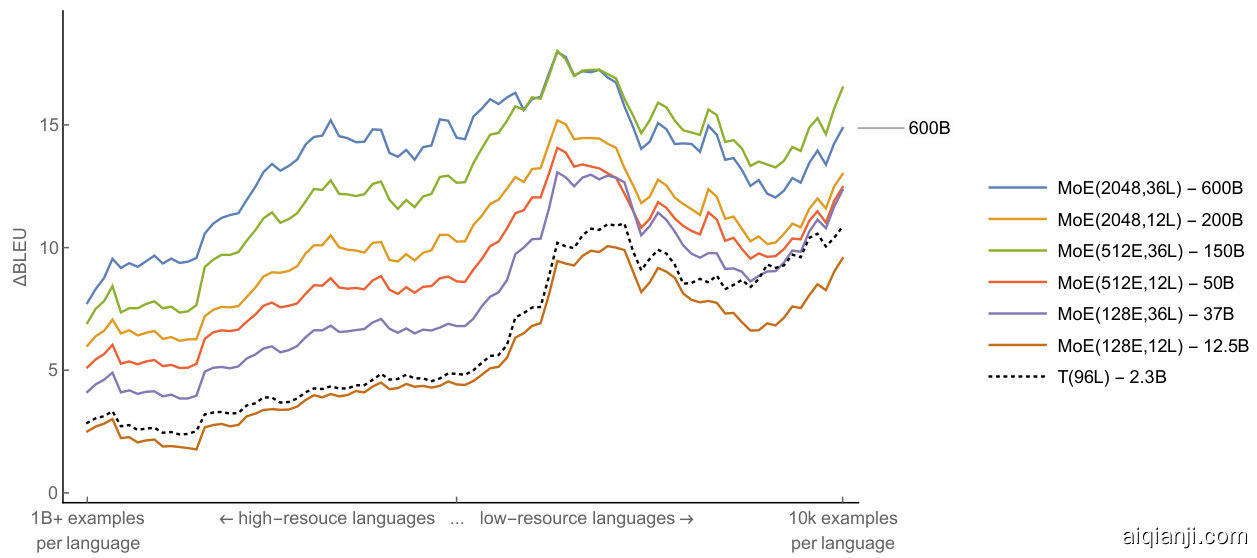
Figure 6: Translation quality comparison of multilingual MoE Transformer models trained with GShard and monolingual baselines. Positions along the $x$ -axis represent languages, raging from highto low-resource. $\Delta$ BLEU represents the quality gain of a single multilingual model compared to a monolingual Transformer model trained and tuned for a specific language. MoE Transformer models trained with GShard are reported with solid trend-lines. Dashed trend-line represents a single 96 layer multilingual Transformer model T(96L) trained with GPipe on same dataset. Each trend-line is smoothed by a sliding window of 10 for clarity. (Best seen in color)
| PI | Model | BLEU avg. | △BLEU avg. | Weights |
| (1) (2) (3) (4) (5) (6) | MoE(2048E,36L) MoE(2048E,12L) MoE(512E,36L) MoE(512E,12L) MoE(128E,36L) MoE(128E,12L) | 44.3 41.3 43.7 40.0 39.0 36.7 | 13.5 10.5 12.9 9.2 8.2 5.9 | 600B 200B 150B 50B 37B 12.5B |
| * * | T(96L) Baselines | 36.9 30.8 | 6.1 | 2.3B 100×0.4B |
图 6: 使用GShard训练的多语言MoE Transformer模型与单语言基线的翻译质量对比。横轴表示从高资源到低资源的语言排序。ΔBLEU表示单一多语言模型相比针对特定语言训练调优的单语言Transformer模型的质量增益。实线趋势线表示GShard训练的MoE Transformer模型,虚线趋势线表示使用GPipe在同一数据集上训练的96层多语言Transformer模型T(96L)。为清晰起见,每条趋势线均采用滑动窗口为10的平滑处理。(建议彩色查看)
| PI | 模型 | BLEU均值 | △BLEU均值 | 参数量 |
|---|---|---|---|---|
| (1) (2) (3) (4) (5) (6) | MoE(2048E,36L) MoE(2048E,12L) MoE(512E,36L) MoE(512E,12L) MoE(128E,36L) MoE(128E,12L) | 44.3 41.3 43.7 40.0 39.0 36.7 | 13.5 10.5 12.9 9.2 8.2 5.9 | 600B 200B 150B 50B 37B 12.5B |
| * * | T(96L) 基线 | 36.9 30.8 | 6.1 | 2.3B 100×0.4B |
Model Details To detail the model specifics, each expert is designed to have the same shape of a regular Transformer feed-forward network, and experts (MoE layers) are distributed once in every other Transformer layer. We tied the number of devices used for training to the number of experts per MoE layer for simplicity, although this is not a requirement. During training, we use float32 for both model weights and activation s in order to ensure training stability. We ran additional s cal ability experiments with MoE(2048E, 60L) with bfloat16 [53] activation s with total of 1 trillion model weights. Although trainable by careful and manual diagnostics, with deep 1 trillion model we encountered several train ability issues with numerical stability, hence did not include the results for the sake of reproducibility. For more model and training details, please see Appendix A.2.
模型细节
为详细说明模型规格,每个专家模块 (expert) 均设计为与标准 Transformer 前馈网络结构相同,且专家模块 (MoE层) 每隔一层 Transformer 层分布一次。为简化流程,我们将训练所用设备数量与每个 MoE 层的专家数量设为相同 (但非强制要求)。训练过程中,模型权重和激活值均采用 float32 格式以确保训练稳定性。我们额外使用 bfloat16 [53] 格式的激活值对 MoE(2048E, 60L) 模型进行了可扩展性实验,该模型总参数量达 1 万亿。尽管通过精细人工诊断可实现训练,但在 1 万亿参数的深度模型中仍遇到数值稳定性导致的训练问题,为保证结果可复现性未纳入相关数据。更多模型及训练细节详见附录 A.2。
4.4 Results
4.4 结果
Before going into the details of training efficiency, we first investigate the effect of various design choices on building MoE Transformer. In order to prune the search space, we explored varying two variables, number of layers in the Transformer encoder-decoder stack (L) and the total number of experts used for every other MoE layer (E). For depth, we tested three different options, 12 (original Transformer depth, which consists of 6 encoder and 6 decoder layers), 36 and 60 layers. For the number of experts that replaces every other feed-forward layer, we also tested three options, namely 128, 512 and 2048 experts. Note that, the number of devices used for training, is fixed to be equal to the number of experts per-layer, using 128, 512 and 2048 cores respectively independent of the depth being experimented. Please also see the detailed description in Table 1 for model configurations.
在深入探讨训练效率之前,我们首先研究了构建MoE Transformer时各种设计选择的影响。为了缩小搜索空间,我们探索了两个变量的变化:Transformer编码器-解码器堆叠的层数(L)以及每隔一个MoE层使用的专家总数(E)。在深度方面,我们测试了三种不同选项:12层(原始Transformer深度,包含6层编码器和6层解码器)、36层和60层。对于替换每隔一个前馈层的专家数量,我们也测试了三种选项:128、512和2048个专家。需要注意的是,用于训练的设备数量固定为每层专家数,分别使用128、512和2048个核心,与实验深度无关。具体模型配置请参见表1中的详细描述。
Table 1: MoE Transformer model family. To achieve desired capacity we i) increased the depth by stacking more layers, ii) increased the width of the network by scaling the number of experts per MoE layer along with number of cores used for training.
| PI | Model | Experts Per-layer | Experts total | TPUv3 Cores | Enc+Dec layers | Weights |
| (1) (2) (3) (4) (5) (6) | MoE(2048E,36L) MoE(2048E,12L) MoE(512E,36L) MoE(512E,12L) MoE(128E,36L) MoE(128E,12L) | 2048 2048 512 512 128 128 | 36684 12228 9216 3072 2304 768 | 2048 2048 512 512 128 128 | 36 12 36 12 36 12 | 600B 200B 150B 50B 37B 12.5B |
| * | MoE(2048E,60L) | 2048 | 61440 | 2048 | 60 | 1T |
表 1: MoE Transformer 模型家族。为实现目标容量,我们采用两种方式:i) 通过堆叠更多层增加深度,ii) 通过扩展每层专家数量及训练核心数增加网络宽度。
| PI | Model | Experts Per-layer | Experts total | TPUv3 Cores | Enc+Dec layers | Weights |
|---|---|---|---|---|---|---|
| (1) (2) (3) (4) (5) (6) | MoE(2048E,36L) MoE(2048E,12L) MoE(512E,36L) MoE(512E,12L) MoE(128E,36L) MoE(128E,12L) | 2048 2048 512 512 128 128 | 36684 12228 9216 3072 2304 768 | 2048 2048 512 512 128 128 | 36 12 36 12 36 12 | 600B 200B 150B 50B 37B 12.5B |
| * | MoE(2048E,60L) | 2048 | 61440 | 2048 | 60 | 1T |
For each experiment (rows of the Table 1), we trained the corresponding MoE Transformer model until it has seen 1 trillion $(10^{12})$ tokens. The model checkpoint at this point is used in the model evaluation. We did not observe any over-fitting patterns by this point in any experiment. Instead, we observed that the training loss continued to improve if we kept training longer. We evaluated BLEU scores that the models achieved for all language pairs on a held-out test set. Figure 6 reports all our results.
对于表1中的每一项实验,我们训练对应的MoE Transformer模型直至其处理完1万亿$(10^{12})$ token。此时保存的模型检查点用于后续评估。所有实验均未在该阶段观察到过拟合现象,相反,继续延长训练时间仍能提升损失函数表现。我们在保留测试集上评估了模型在所有语言对中取得的BLEU分数,完整结果见图6。
Here we share a qualitative analysis for each experiment and discuss the implication of each setup on high- and low-resource languages in order to track our progress towards universal translation. To ground the forthcoming analysis, it is worth restating the expected behavior of the underlying quality gains. In order to improve the quality for both high- and low-resource languages simultaneously within a single model, scaled models must mitigate capacity bottleneck issue by allocating enough capacity to high-resource tasks, while amplifying the positive transfer towards low-resource tasks by facilitating sufficient parameter sharing. We loosely relate the expected learning dynamics of such systems with the long-standing memorization and generalization dilemma, which is recently studied along the lines of width vs depth scaling efforts [54]. Not only do we expect our models to generalize better to the held-out test sets, we also expect them to exhibit high transfer capability across languages as another manifestation of generalization performance [55].
我们在此分享每项实验的定性分析,并探讨不同设置对高资源和低资源语言的影响,以追踪我们在通用翻译领域的进展。为了支撑后续分析,有必要重申模型质量提升的预期表现:要在一个模型中同时提升高资源和低资源语言的翻译质量,规模化模型必须通过为高资源任务分配足够容量来缓解能力瓶颈问题,同时通过促进充分的参数共享来增强向低资源任务的正向迁移。我们将这类系统的预期学习动态与长期存在的记忆与泛化困境相联系,该问题近期正沿着宽度与深度扩展的研究方向被探讨[54]。我们不仅期望模型在保留测试集上展现更好的泛化能力,还期望其通过跨语言的高迁移能力来体现泛化性能的另一种表现形式[55]。
Deeper Models Bring Consistent Quality Gains Across the Board We first investigate the relationship between the model depth and the model quality for both high- and low-resource languages. Three different experiments are conducted in order to test the generalization performance, while keeping the number of experts per-layer fixed. With an increasing number of per-layer experts for each experiment (128, 512 and 2048), we tripled the depth of the network for each expert size, from 12 to 36. This resulted in three groups where experts per-layer fixed but three times the depth within each group:
更深层的模型带来全面一致的质量提升
我们首先研究了模型深度与模型质量之间的关系,涵盖高资源和低资源语言。为测试泛化性能,我们在保持每层专家数量固定的情况下进行了三项不同实验。随着每项实验中每层专家数量的增加(128、512和2048),我们将每种专家规模对应的网络深度从12层增至36层,形成三组实验:每组保持每层专家数固定,但深度增加三倍。
For each configuration shown in Fig. 6, we observed that increasing the depth (L) while keeping the experts per-layer (E) fixed, brings consistent gains for both low and high resourced languages (upwards $\Delta$ shift along the $y$ -axis), almost with a constant additive factor every time we scale the depth from 12L to 36L (2-to-3 BLEU points on average as shown in the last column of Table 3).
对于图6所示的每种配置,我们观察到在保持每层专家数(E)不变的情况下增加深度(L),能为低资源和高资源语言带来持续增益(y轴上的$\Delta$上升趋势)。当深度从12层扩展到36层时,这种提升几乎呈现恒定累加效应(如表3最后一列所示,平均带来2-3个BLEU分数提升)。
Relaxing the Capacity Bottleneck Grants Pronounced Quality Gains Earlier in Section 4.1 we highlighted the influence of the capacity bottleneck on task interference, resulting in degraded quality especially for high resourced languages. Later we alleviated this complication by increasing the number of experts per-layer, which in return resulted in a dramatic increase in the number of parameters (weight) of the models studied. Here we investigate whether this so called capacity bottleneck is distinctly observable and explore the impact on model quality and efficiency once it is relaxed. To that end, we first consider three models with identical depths (12L), with increasing number of experts per-layer: 128, 512 and 2048. As we increase the number of experts per-layer from 128 to 512 by a factor of four, we notice a large jump in model quality, $+3.3$ average BLEU score across 100 languages. However again by four folds scaling of the number of experts per-layer, from 512 to 2048, yields only $+1.3$ average BLEU scores. Despite the significant quality improvement, this drop in gains hints the emergence of diminishing returns.
放宽容量瓶颈可在早期带来显著质量提升
在4.1节中我们强调了容量瓶颈对任务干扰的影响,这会导致质量下降,尤其是对高资源语言。随后我们通过增加每层专家数量缓解了这一复杂问题,反过来也导致研究模型的参数量(权重)急剧增加。此处我们探究这种所谓的容量瓶颈是否明显可观测,并探索其放宽后对模型质量和效率的影响。为此,我们首先考虑三个深度相同(12层)、每层专家数量递增(128/512/2048)的模型。当每层专家数量从128增至512(4倍)时,模型质量出现大幅跃升,100种语言的平均BLEU分数提升+3.3。然而当专家数量再次4倍增长(从512到2048)时,平均BLEU分数仅提升+1.3。尽管质量显著改善,但增益下降暗示了收益递减现象的出现。
Speculative ly, the capacity bottleneck is expected to be residing between 128 to 512 experts, for the particular para me tri z ation, number of languages and the amount of training data used in our experimental setup. Once the bottleneck is relaxed, models enjoy successive scaling of the depth, which can be seen by comparing 12 versus 36 layer models both with 128 experts. Interestingly increasing the depth does not help as much if the capacity bottleneck is not relaxed.
推测来看,在我们的实验设置所采用的特定参数化方案、语言数量及训练数据量条件下,容量瓶颈预计存在于128至512个专家(expert)之间。一旦突破该瓶颈,模型就能实现深度的持续扩展——通过比较具有128个专家的12层与36层模型即可观察到这一现象。值得注意的是,若容量瓶颈未被突破,单纯增加深度带来的收益将显著受限。
Having More Experts Improve Quality Especially for High-Resourced Tasks Another dimension that could shed light on the quality gains of scaling in multi-task models is the contrast between high and low resource language improvements. As mentioned before, low resourced languages benefit from transfer while high resource languages seek for added capacity. Next we examine the effect of increasing the experts per-layer while fixing the depth.
增加专家数量提升质量 尤其针对高资源任务
另一个能揭示多任务模型扩展质量提升的维度是高资源与低资源语言改进效果的对比。如前所述,低资源语言受益于迁移学习,而高资源语言则需要额外容量。接下来我们研究在固定深度情况下,增加每层专家数量的效果。
As can be seen in Figure 6, for 12 layer models increase in the expert number yields larger gains for high resourced languages as opposed to earlier revealed diminishing returns for low-resourced languages. A similar pattern is observed also for 36 layer models. While adding more experts relaxes the capacity bottleneck, at the same time it reduces the amount of transfer due to a reduction of the shared sub-networks.
如图 6 所示,对于 12 层模型,专家数量的增加为高资源语言带来了更大的收益,而低资源语言则呈现出先前揭示的收益递减现象。36 层模型也观察到类似模式。虽然增加专家数量缓解了容量瓶颈,但同时由于共享子网络的减少,也降低了迁移量。
Deep-Dense Models are Better at Positive Transfer towards Low-Resource Tasks Lastly we look into the impact of the depth on low-resourced tasks as a loose corollary to our previous experiment. In order to do so, we include a dense model with 96 layers T(96L) trained with GPipe on the same data into our analysis. We compare T(96L) with the shallow MoE(128E, 12L) model. While the gap between the two models measured to be almost constant for the majority of the high-to-mid resourced languages, the gap grows in favor of the dense-deep T(96L) model as we get into the low-resourced regime. Following our previous statement, as the proportion of the shared sub-networks across tasks increase, which is $100%$ for dense T(96L), the bandwidth for transfer gets maximized and results in a comparably better quality against its shallow counterpart. Also notice that, the same transfer quality to the low-resourced languages can be achieved with MoE(36E, 128L) which contains 37 billion parameters.
深度密集模型在低资源任务的正向迁移中表现更优
最后,我们探讨深度对低资源任务的影响,作为先前实验的延伸推论。为此,我们在分析中加入了采用GPipe框架训练、包含96层的密集模型T(96L)。通过对比T(96L)与浅层MoE(128E, 12L)模型发现:在中高资源语言中,两者的性能差距基本保持恒定;但当进入低资源领域时,深度密集的T(96L)模型优势显著扩大。正如前文所述,当任务间共享子网络比例提升时(密集模型T(96L)可达100%),迁移带宽达到最大化,从而使该模型相较浅层版本获得更优性能。值得注意的是,参数量达370亿的MoE(36E, 128L)模型也能实现同等水平的低资源语言迁移质量。
We conjecture that, increasing the depth might potentially increase the extent of transfer to lowresource tasks hence generalize better along that axis. But we also want to highlight that the models in comparison have a disproportionate training resource requirements. We again want to promote the importance of training efficiency, which is the very topic we studied next.
我们推测,增加深度可能会提升对低资源任务的迁移程度,从而在该维度上实现更好的泛化性能。但需要指出的是,对比模型的训练资源需求存在显著差异。我们再次强调训练效率的重要性,这也正是接下来要研究的核心课题。
4.5 Training Efficiency
4.5 训练效率
In this section we focus on the training efficiency of MoE Transformer models. So far, we have seen empirical evidence how scaling the models along various axes bring dramatic quality gains, and studied the factors affecting the extent of the improvements. In order to measure the training efficiency, we first keep track of the number of tokens being processed to reach a certain training loss and second we keep track of the wall-clock time for a model to process certain number of tokens. Note that, we focus on the training time and training ${\mathrm{loss}}^{13}$ while varying other factors, as opposed to test error, which we analyzed in the previous section.
在本节中,我们重点研究MoE Transformer模型的训练效率。截至目前,我们已经通过实证数据观察到模型在不同维度上的扩展如何带来显著的质量提升,并分析了影响改进幅度的关键因素。为衡量训练效率,我们首先追踪模型达到特定训练损失时处理的token数量,其次记录模型处理固定数量token所需的实际耗时。需要注意的是,我们关注的是训练时间和训练损失${\mathrm{loss}}^{13}$的变化规律(通过调整其他变量实现),这与前一节分析的测试误差形成对比。
Deeper models are more sample efficient, converge faster with fewer examples It has been shown that, deeper models are better at sample efficiency, reaching better training/test error given the same amount of training examples [15, 56], commonly attributed to the acceleration effect of overpara me tri z ation [1]. We empirically test the hypothesis again using GShard with MoE Transformers and share trade-offs for models that are not only deep, but also sparsely activated.
更深的模型样本效率更高,用更少的样本就能更快收敛
研究表明,在相同训练样本量下,更深的模型具有更好的样本效率,能达到更优的训练/测试误差 [15, 56],这通常归因于过参数化(overparameterization)的加速效应 [1]。我们使用GShard框架下的MoE Transformer再次实证检验这一假设,并分享了不仅深度更深、还具有稀疏激活特性的模型权衡方案。
For this purpose, we compare number of tokens being processed by each model to reach a preset training loss. A general trend we observe from Table 2 is that, MoE Transformer models with 3 times the depth need 2 to 3 times fewer tokens to reach the preset training loss thresholds. For example MoE(128E, 12L) takes 3 times the number of tokens to reach 0.7 training cross-entropy compared to MoE(128E, 36L), (6) vs (5). We observe a similar trend for models with 512 and 2048 experts, (4) vs (3) and (2) vs (1).
为此,我们比较了各模型为达到预设训练损失所需处理的token数量。从表2中观察到的总体趋势是:深度增加3倍的MoE Transformer模型,达到预设训练损失阈值所需的token数量减少2到3倍。例如,MoE(128E, 12L)达到0.7训练交叉熵所需的token数量是MoE(128E, 36L)的3倍(6 vs 5)。在512和2048专家的模型中我们也观察到类似趋势(4 vs 3和2 vs 1)。
| PI | Model | Cores | Billiontokensto cross-entropy of | ||
| (1) (2) (3) (4) | MoE(2048E,36L) MoE(2048E,12L) MoE(512E,36L) | 2048 2048 512 512 | 0.7 82 176 66 | 0.6 175 484 170 | 0.5 542 1780 567 |
Table 2: The number of tokens have been seen by a model during training to reach three different cross-entropy loss. A general trend is that deeper models are more sample efficient and converge faster than the comparable shallow ones.
表 2: 模型在训练过程中达到三种不同交叉熵损失时所见过的token数量。总体趋势是,较深的模型比同等条件下较浅的模型具有更高的样本效率且收敛更快。
| PI | 模型 | 核心数 | 交叉熵达到的十亿token数 (0.7) | 交叉熵达到的十亿token数 (0.6) | 交叉熵达到的十亿token数 (0.5) |
|---|---|---|---|---|---|
| (1) (2) (3) (4) | MoE(2048E,36L) MoE(2048E,12L) MoE(512E,36L) | 2048 2048 512 512 | 82 176 66 | 175 484 170 | 542 1780 567 |
Another intriguing observation from Table 2, is again related to the presence of capacity bottleneck. Comparing the models with same depth, (5), (3) and (1), we notice a significant drop in the number of tokens required to reach training loss of 0.7, as we transition from 128 to 512 number of experts. Practically that is where we observed the capacity bottleneck was residing, aligning with the hypothesis in Section 4.4. After this phase shift, models with ample capacity tend to exhibit similar sample efficiency characteristics, as in models (3) and (1).
从表2中另一个有趣的观察再次与容量瓶颈的存在相关。比较相同深度(5)、(3)和(1)的模型时,我们注意到当专家数量从128增加到512时,达到训练损失0.7所需的token数量显著下降。实际上这正是我们观察到容量瓶颈存在的位置,与第4.4节的假设一致。经过这个相变后,具有充足容量的模型(如模型(3)和(1))往往表现出相似的样本效率特征。
Largest model (600B) can be trained under 4 days achieving the best quality Next we delve deeper into the interaction between model size and wall-clock time spent for training. We monitor number of TPU cores being used, training steps per-second, total number of tokens per batch, TPU core years14, and actual wall-clock time spent in days for training (see Table 3 columns respectively).
最大模型(6000亿参数)可在4天内完成训练并达到最佳质量
接下来我们深入探讨模型规模与训练耗时之间的关系。我们监测了以下指标:使用的TPU核心数量、每秒训练步数、每批次token总数、TPU核心年[14]以及实际训练耗时(天数)(参见表3各列)。
We start with investigating one of the largest models we trained, MoE(2048E, 36L) with 600 billion parameters, model with id (1). Having utilized 2048 TPU cores for 4 days, this model achieves the best translation quality in terms of average BLEU, but also takes a total of 22.4 TPU years to train. While we have not seen any signs that the quality improvements plateau as we scale up our models, we strive for finding cost-effective solutions for scaling.
我们首先研究了所训练的最大模型之一——具有6000亿参数的MoE(2048E, 36L)模型(编号1)。该模型使用2048个TPU核心训练4天,在平均BLEU指标上实现了最佳翻译质量,但总训练耗时达22.4个TPU年。虽然目前尚未观察到模型规模扩大时质量提升出现平台期,但我们仍在寻求更具成本效益的扩展方案。
Results in Table 3 again validates scaling with conditional computation is way more practical compared to dense scaling. Given the same number of TPU cores used by (1), the dense scaling variant, T(96L), appears to be taking more than ten times to train (235 TPU core years), while trailing behind in terms of model quality compared to models trained with GShard.
表 3 中的结果再次验证了条件计算 (conditional computation) 的扩展性相比密集扩展 (dense scaling) 更为实用。在使用相同数量 TPU 核心的情况下,密集扩展变体 T(96L) 的训练耗时超过十倍 (235 TPU 核心年) ,且模型质量仍落后于使用 GShard 训练的模型。
| PI | Model | Cores | Steps per sec. | Batchsz. (Tokens) | TPUcore years | Training time (days) | BLEU avg. |
| (1) (2) (3) (4) (5) | MoE(2048E,36L) MoE(2048E,12L) MoE(512E,36L) MoE(512E,12L) MoE(128E,36L) | 2048 2048 512 512 128 | 0.72 2.15 1.05 3.28 0.67 | 4M 4M 1M 1M 1M | 22.4 7.5 15.5 4.9 6.1 | 4.0 1.4 11.0 3.5 | 44.3 41.3 43.7 40.0 |
| (6) * | MoE(128E,12L) T(96L) | 128 2048 | 2.16 | 1M 4M | 1.9 ~235.5 | 17.3 5.4 ~42 | 39.0 36.7 36.9 |
Table 3: Performance of MoE models with different number of experts and layers.
| PI | 模型 | 核心数 | 每秒步数 | 批量大小 (Token) | TPU核心年 | 训练时间 (天) | BLEU平均分 |
|---|---|---|---|---|---|---|---|
| (1)(2)(3)(4)(5) | MoE(2048E,36L) | ||||||
| MoE(2048E,12L) | |||||||
| MoE(512E,36L) | |||||||
| MoE(512E,12L) | |||||||
| MoE(128E,36L) | 2048 | ||||||
| 2048 | |||||||
| 512 | |||||||
| 512 | |||||||
| 128 | 0.72 | ||||||
| 2.15 | |||||||
| 1.05 | |||||||
| 3.28 | |||||||
| 0.67 | 4M | ||||||
| 4M | |||||||
| 1M | |||||||
| 1M | |||||||
| 1M | 22.4 | ||||||
| 7.5 | |||||||
| 15.5 | |||||||
| 4.9 | |||||||
| 6.1 | 4.0 | ||||||
| 1.4 | |||||||
| 11.0 | |||||||
| 3.5 |
- | 44.3
41.3
43.7
40.0 - |
| (6)* | MoE(128E,12L)
T(96L) | 128
2048 | 2.16 - | 1M
4M | 1.9
~235.5 | 17.3
5.4
~42 | 39.0
36.7
36.9 |
表 3: 不同专家数和层数的MoE模型性能。
In this section, we benchmarked GShard with MoE Transformers applications to multilingual machine translation (in particular to M4). We identified variables that are affecting the end result, such as capacity bottleneck, positive transfer and training efficiency, and provided experimental results in order to reveal the interplay between them. Next we will delve deep into performance related topics of GShard, such as memory and runtime efficiency and communication benchmarks.
在本节中,我们使用MoE Transformer对GShard进行了多语言机器翻译(特别是M4)的基准测试。我们识别了影响最终结果的关键变量,例如容量瓶颈(capacity bottleneck)、正向迁移(positive transfer)和训练效率,并通过实验结果揭示它们之间的相互作用关系。接下来我们将深入探讨GShard的性能相关主题,包括内存与运行时效率、通信基准测试等。

Figure 7: Per-device memory consumption in gigabytes.
图 7: 各设备内存消耗 (单位: GB)。
5 Performance and Memory Consumption
5 性能与内存消耗
This section discusses how well GShard achieves computation and memory efficiency on the TPU platform. Our measurement and analysis show that the device memory consumption is roughly constant when we increase the number of devices and experts, and the step time grows sub linearly, i.e., $1.7\mathbf{X}$ execution time increase when we scale the model by 16x from 128 devices to 2048 devices. We also provide micro benchmarks and analyses for a variety of partitioned operators, which could guide use cases beyond this paper.
本节讨论GShard在TPU平台上实现的计算和内存效率。我们的测量与分析表明,当增加设备和专家数量时,设备内存消耗大致保持恒定,而单步时间呈次线性增长——即从128台设备扩展到2048台设备(规模扩大16倍)时,执行时间仅增加$1.7\mathbf{X}$。我们还提供了多种分区算子的微观基准测试与分析,这些结果可指导本文范围之外的应用场景。
5.1 Memory Efficiency and S cal ability
5.1 内存效率与可扩展性
In the GShard model, there are mainly three types of memory usage, all of which have constant per-device sizes after SPMD partitioning, when the number of experts increases.
在GShard模型中,主要有三种内存使用类型,当专家数量增加时,经过SPMD分区后它们都保持每个设备上的恒定大小。
The $O(1)$ memory scaling is demonstrated in Figure 7, which shows the per-device memory usage distribution for different models. With a fixed number of layers, both weight memory and activation memory stay constant when the number of experts increases.
$O(1)$ 内存扩展特性如图 7 所示,该图展示了不同模型的单设备内存使用分布。在固定层数的情况下,当专家数量增加时,权重内存和激活内存均保持恒定。
On this other hand, weight memory and activation memory both scale linearly with the number of layers. When the memory requirement exceeds available memory on each device, compiler-based re materialization will automatically recompute part of the activation s in the backward pass in order to reduce peak activation memory. This is why the activation size for MoE(2048E, 60L) is smaller than MoE(2048E, 36L). The overhead of re materialization is also optimized, e.g. only $28%$ and $34%$ of the total cycles are spent on re computation for 36L and 60L models respectively, and $0%$ for 12L and 24L since they fit in device memory without re materialization.
另一方面,权重内存和激活内存都与层数呈线性增长。当内存需求超过每个设备的可用内存时,基于编译器的重计算 (re-materialization) 会在反向传播过程中自动重新计算部分激活值,以降低峰值激活内存。这就是为什么 MoE(2048E, 60L) 的激活大小比 MoE(2048E, 36L) 更小。重计算的开销也经过优化,例如 36 层和 60 层模型分别仅花费总计算周期的 $28%$ 和 $34%$ 进行重计算,而 12 层和 24 层模型由于无需重计算即可适配设备内存,开销为 $0%$。

Figure 8: Measured vs roofline execution time breakdown. Only the forward pass is shown, and the backward pass has similar breakdown. “MoE dispatch and combine” represents cross-partition communication with AllToAll.
图 8: 实测与理论极限执行时间分解对比。仅展示前向传播过程,反向传播具有类似分解模式。"MoE调度与组合"表示通过AllToAll进行的跨分区通信。
5.2 Runtime Efficiency and S cal ability
5.2 运行时效率与可扩展性
Figure 8 shows the breakdown of execution time for an MoE layer and its adjacent Transformer layer. It also compares the achieved performance to a roofline, which is estimated by assuming compute-, memory-, or communication-bounded operations can achieve $100%$ of the peak FLOPS, memory bandwidth, or interconnect bandwidth. This is a very optimistic estimate as many operators are bounded by a mixed set of resources. At a smaller scale (128 experts), our model can achieve $>70%$ of the roofline performance. The device time increases by $1.7\mathbf{x}$ when we scale the model to 16x larger (2048 experts), and can still achieve $48%$ of the roofline performance.
图 8 展示了混合专家层 (MoE) 及其相邻 Transformer 层的执行时间分解,同时将实际性能与理论峰值 (roofline) 进行对比。该理论峰值通过假设计算密集型、内存密集型或通信密集型操作可分别达到 $100%$ 的峰值算力 (FLOPS)、内存带宽或互连带宽估算得出(此为非常乐观的估计,因为多数算子受多种资源共同限制)。在小规模场景(128个专家)下,我们的模型能达到 $>70%$ 的理论峰值性能。当模型规模扩大16倍(2048个专家)时,设备耗时增加 $1.7\mathbf{x}$,但仍可保持 $48%$ 的理论峰值性能。
Before analyzing performance s cal ability, we recall the size scaling of relevant tensor dimensions as discussed in Section 3.1. With $D$ devices, the number of experts $E$ and the group count $G$ are both set to $O(D)$ . The fractional per-group expert capacity $C$ is set to $O(1/D)$ . This setup cannot scale indefinitely, since $C$ needs to be at least 1, but it is good enough to scale to thousands of experts.
在分析性能扩展能力之前,我们先回顾第3.1节讨论的相关张量维度的尺寸缩放关系。当设备数为$D$时,专家数量$E$和分组数$G$都设置为$O(D)$。每组的专家容量分数$C$设置为$O(1/D)$。这种设置无法无限扩展,因为$C$至少需要为1,但对于扩展到数千名专家已经足够。
Transformer layers and MoE feed-forward layer These are the dense parts of the model, which are designed to achieve peak TPU utilization. On each device, these computations also have a constant cost when we scale to more experts. Feed-forward layers and Transformer projections are mainly large matrix multiplications that utilize the TPU’s matrix unit well. These operations have achieved $>85%$ peak FLOPS in our experiment. The attention operations are composed of mainly batch matmuls, which are bounded by memory bandwidth when sequence lengths are small. As a result, in our experiments attention operations only achieved $>30%$ peak FLOPS.
Transformer层和MoE前馈层
这些是模型的密集计算部分,旨在实现TPU的峰值利用率。在每台设备上,当我们扩展到更多专家时,这些计算也具有恒定成本。前馈层和Transformer投影层主要是大型矩阵乘法,能很好地利用TPU的矩阵单元。在我们的实验中,这些操作的峰值FLOPS利用率达到了$>85%$。注意力操作主要由批量矩阵乘法组成,当序列长度较小时受限于内存带宽。因此,在我们的实验中注意力操作的峰值FLOPS利用率仅达到$>30%$。
Gate computation In Figure 8, “Gate Einsum” represents the first two and the last Einsums in Algorithm 2. The first Einsum is the projection that calculates per-expert input to softmax. It has an $O(D)$ cost, but it is a very small part of the layer. The other two Einsums are dispatching tokens and combining expert results. They effectively implement Gather with one-hot matrices, which are more expensive, but with constant $O(G C)\stackrel{\cdot}{=}O\bar{(}1)$ cost that is independent from the number of experts. The execution time of these Einsums increases by around $2\mathbf{x}$ when we scale from 128 to 2048 experts (16x).
门控计算
在图 8 中,"Gate Einsum" 表示算法 2 中的前两个和最后一个 Einsum。第一个 Einsum 是计算每个专家输入到 softmax 的投影,其复杂度为 $O(D)$,但这只是层中非常小的一部分。另外两个 Einsum 用于分发 token 和合并专家结果。它们实际上是通过 one-hot 矩阵实现 Gather 操作,虽然计算开销更大,但具有恒定的 $O(G C)\stackrel{\cdot}{=}O\bar{(}1)$ 复杂度,与专家数量无关。当专家数量从 128 扩展到 2048 (16 倍) 时,这些 Einsum 的执行时间增加了约 $2\mathbf{x}$。
The remaining per-device gating computation involves many general-purpose computations like ArgMax and Cumsum, which are either memory-bound or even sequential in nature, thus not designed to utilize TPUs well. The majority of the time is spent on sequential Cumsum operations to invert one-hot matrices that represent selected experts for each token to one-hot matrices that represent selected tokens for each expert. The linear complexity of Cumsum is demonstrated in Figure 8. This part of the gating computation also has an $O(D)$ cost, but fortunately, similar to the Einsum before softmax, it has a very small constant factor. It has negligible execution time with 128 experts, and takes less than $10%$ of the total time spent in the MoE and Transformer layers with 2048 experts.
剩余的设备级门控计算涉及许多通用计算操作,如ArgMax和Cumsum,这些操作本质上是内存受限甚至顺序执行的,因此无法充分利用TPU的性能。大部分时间消耗在将表示每个token所选专家的独热矩阵转换为表示每个专家所选token的独热矩阵的顺序Cumsum操作上。图8展示了Cumsum的线性复杂度。这部分门控计算同样存在$O(D)$的时间复杂度,但幸运的是,与softmax前的Einsum类似,其常数因子极小。在使用128个专家时执行时间可忽略不计,在使用2048个专家时仅占MoE层和Transformer层总耗时的不到$10%$。
The most significant part of gating is communication, shown as “MoE dispatch and combine” in Figure 8. These are AllToAll operators, and as we will discuss in Section 5.3, their cost is $O({\sqrt{D}})$ . When the number experts grows 16x from 128 to 2048, the execution time increases by about $3.75\mathbf{X}$ , and their proportion of execution time in the MoE and Transformer increases from $16%$ to $36%$ .
门控机制最重要的部分是通信,如图 8 中的 "MoE 分发与合并" 所示。这些是 AllToAll 运算符,正如我们将在 5.3 节讨论的那样,其成本为 $O({\sqrt{D}})$ 。当专家数量从 128 个增长 16 倍至 2048 个时,执行时间增加约 $3.75\mathbf{X}$ ,其在 MoE 和 Transformer 中的执行时间占比从 $16%$ 上升至 $36%$ 。
5.3 Communication Micro benchmarks and Per-Operator S cal ability
5.3 通信微基准测试与单算子可扩展性
In this section, we measure and analyze the performance s cal ability of the SPMD partition er for basic operators, which can be used to guide use cases beyond the MoE model presented in this paper.
在本节中,我们测量并分析了SPMD分区器对基础算子的性能扩展能力,这些发现可指导本文所述MoE模型之外的其他应用场景。
Performance scaling of communication primitives Two critical collective communication operators in the MoE model are AllReduce and AllToAll. AllReduce is used in accumulating partial results, and AllToAll is used in resharding (Section 3.3.2). Figure 9 shows their performance s cal ability from 16 to 2048 partitions. AllReduce on TPU has an execution time independent from the number of devices. The variance in Figure 9 is due to specifics of each topology, e.g., whether it is a square or a rectangle, and whether it is a torus or a mesh.
通信原语的性能扩展
MoE模型中两个关键的集体通信操作符是AllReduce和AllToAll。AllReduce用于累加部分结果,AllToAll用于重分片(见3.3.2节)。图9展示了它们从16到2048分区的性能扩展能力。TPU上的AllReduce执行时间与设备数量无关。图9中的差异源于每种拓扑的具体特性,例如是正方形还是矩形,是环形还是网状结构。
AllToAll, on the other hand, gets more expensive as the number of partitions grows, but in a sublinear manner. On our 2D TPU cluster, AllToAll cost is roughly $O({\sqrt{D}})$ , where $D$ is the number of partitions. This is because with a fixed amount of data each partition sends (8MB or 32MB in Figure 9), the total amount of data that all partitions send is $d=O(D)$ . Meanwhile, each data piece needs to travel $h=O({\sqrt{D}})$ hops on average, and there are overall $l=O(D)$ device-to-device links in the network. Therefore, if it is bandwidth-bound, the execution time of an AllToAll is
另一方面,AllToAll 的成本随着分区数量增加而上升,但呈次线性增长。在我们的 2D TPU 集群中,AllToAll 成本约为 $O({\sqrt{D}})$ ,其中 $D$ 表示分区数量。这是因为每个分区发送固定数据量 (图 9 中为 8MB 或 32MB) 时,所有分区发送的数据总量为 $d=O(D)$ 。同时,每个数据块平均需要经过 $h=O({\sqrt{D}})$ 跳传输,而网络中总共存在 $l=O(D)$ 条设备间链路。因此,若受带宽限制,AllToAll 的执行时间为
$$
t=\frac{d h}{l}=O(\frac{D\sqrt{D}}{D})=O(\sqrt{D}).
$$
$$
t=\frac{d h}{l}=O(\frac{D\sqrt{D}}{D})=O(\sqrt{D}).
$$
Even if it is latency-bound, the execution time will still be $O(h)=O({\sqrt{D}})$ . Comparing 2048 partitions and 16 partitions, while $D$ grows by 128 times, the execution time of AllToAll only increases by 9 times. This enables us to use resharding to efficiently implement cross-partition dispatching (Figure 4a).
即使受限于延迟,执行时间仍为 $O(h)=O({\sqrt{D}})$ 。比较2048个分区和16个分区的情况,当 $D$ 增长128倍时,AllToAll的执行时间仅增加9倍。这使得我们能够通过重分片高效实现跨分区调度 (图4a)。
AllGather and Collective Permute are easier to analyze. AllGather’s output is $D$ larger than the input, and if we fix input size, then its communication cost is $O(D)$ . Collective Permute has a oneto-one communication pattern, and with reasonable device arrangement where the source-destination pairs are close, its cost is $O(1)$ for a fixed input size.
AllGather和Collective Permute更容易分析。AllGather的输出比输入大$D$倍,若固定输入大小,其通信成本为$O(D)$。Collective Permute采用一对一通信模式,在源-目标对距离较近的合理设备布局下,固定输入大小时其成本为$O(1)$。
Table 4: S cal ability of partitioned operators. Abbreviation for communication primitives: AR: AllReduce, AG: AllGather, CP: Collective Permute, AA: AllToAll. *This is the dispatch Einsum in our model, where we set C to $O(1/D)$ . $\ast\ast_ {\mathrm{I/0}}$ are the input/output feature dimensions, B is the batch dimension, $\texttt{X/Y}$ are input spatial dimensions, and $\mathbf{x}/\mathbf{y}$ are the kernal spatial dimensions.
| O(D) Dimensions | Total Compute | Per-partition | ||
| Compute | Communication | |||
| Add(A,A->A) | A | O(D) | 0(1) | 0 |
| Matmul(AB,BC->AC) | B | O(D) | 0(1) | O(1) AR |
| Matmul(AB,BC->AC) | A | O(D) | 0(1) | 0 |
| Matmul(AB,BC->AC) | A,B | O(D2) | O(D) | O(D) AG or CP |
| Matmul(AB,BC->AC) | A,C | O(D2) | O(D) | O(D) AG or CP |
| Reduce(AB->A) | A | O(D) | 0(1) | 0 |
| Reduce(AB->B) | A | O(D) | 0(1) | 0(1) AR |
| Einsum(GSEC,GSM->EGCM) | G,E* | O(D) | 0(1) | O(VD) AA |
| Convolution(BIXY,xyIO->BOXY) | **X | O(D) | 0(1) | 0(1) CP |
表 4: 分区算子的可扩展性。通信原语缩写: AR: AllReduce, AG: AllGather, CP: Collective Permute, AA: AllToAll。*这是我们模型中的调度Einsum,其中我们将C设置为$O(1/D)$。**I/O是输入/输出特征维度,B是批次维度,X/Y是输入空间维度,x/y是核空间维度。
| O(D)维度 | 总计算量 | 每分区 | |
|---|---|---|---|
| 计算量 | |||
| Add(A,A->A) | A | O(D) | 0(1) |
| Matmul(AB,BC->AC) | B | O(D) | 0(1) |
| Matmul(AB,BC->AC) | A | O(D) | 0(1) |
| Matmul(AB,BC->AC) | A,B | O(D2) | O(D) |
| Matmul(AB,BC->AC) | A,C | O(D2) | O(D) |
| Reduce(AB->A) | A | O(D) | 0(1) |
| Reduce(AB->B) | A | O(D) | 0(1) |
| Einsum(GSEC,GSM->EGCM) | G,E* | O(D) | 0(1) |
| Convolution(BIXY,xyIO->BOXY) | **X | O(D) | 0(1) |

Figure 9: Performance scaling of communication, AllReduce and AllToAll. Log scale on both axes. AllReduce cost is roughly $O(1)$ , and AllToAll cost is roughly $O({\sqrt{D}})$ , where $D$ is the number of partitions. We measure their performance with 8MB and 32MB data. For AllToAll, that means each partition initially has 8MB (or 32MB) data, then divides it to $D$ pieces, and sends each piece to a different receiving partition.
图 9: 通信、AllReduce和AllToAll的性能扩展。双对数坐标轴。AllReduce成本约为 $O(1)$ ,AllToAll成本约为 $O({\sqrt{D}})$ ,其中 $D$ 为分区数量。我们使用8MB和32MB数据测量其性能。对于AllToAll,这意味着每个分区初始持有8MB(或32MB)数据,随后将其分割为 $D$ 份并分别发送至不同接收分区。
Partitioned operator s cal ability We summarize the performance s cal ability for common operators using GShard in Table 4. It contains the Einsum/Matmul examples in Section 3.3.2, and also other common operators like Convolution and Reduce. The table includes the local compute on each partition, as well as the required communication based on our analysis above.
分区算子可扩展性
我们在表4中总结了使用GShard时常见算子的性能可扩展性。该表包含第3.3.2节中的Einsum/Matmul示例,以及卷积(Convolution)和归约(Reduce)等其他常见算子。表中列出了每个分区的本地计算量,以及基于上述分析所需的通信量。
Most operators in Table 4 have sublinear s cal ability in terms of both compute and communication, which is consistent with our performance measurement of the MoE model. The $O(1)$ scaling of spatially partitioned convolutions also demonstrates the efficiency of GShard for image partitioning (Appendix A.4).
表4中的大多数算子都具有计算和通信方面的次线性扩展能力,这与我们对MoE模型的性能测量结果一致。空间分区卷积的$O(1)$扩展性也证明了GShard在图像分区方面的效率(附录A.4)。
However, the last two Matmul operators in Table 4 have $O(D)$ scaling of per-partition compute and communication, where they have unmatched sharding in the operands. This is not due to inefficiency in the partitioning algorithm, but because the total compute in the full operator is very large $(O(D^{2}))$ . Different partitioning strategies can be used for these cases, producing different communication primitives: replicating one operand will result in AllGather (requiring the replicated operand to fit in device memory), while slicing in a loop (Figure 4c) will result in Collective Permute.
然而,表4中最后两个矩阵乘法(Matmul)算子的每个分区计算和通信复杂度为$O(D)$,其操作数存在不匹配的分片情况。这并非分区算法效率不足所致,而是因为完整算子的总计算量极大$(O(D^{2}))$。针对此类情况可采用不同分区策略,从而产生不同的通信原语:复制其中一个操作数将产生AllGather(要求复制的操作数能放入设备内存),而循环切片(图4c)则会产生Collective Permute。
6 Related Work
6 相关工作
Neural networks Deep learning models have been very successful in advancing sub-fields of artificial intelligence. For years, the fields have been continuously reporting new state of the art results using varieties of model architectures for computer vision tasks [57, 58, 7], for natural language understanding tasks [59, 60, 61], for speech recognition and synthesis tasks [62, 63, 64, 65, 66]. More recently, attention-based Transformer models further advanced state of the art of these fields [10, 4].
神经网络
深度学习模型在推动人工智能各子领域发展方面取得了巨大成功。多年来,该领域持续报告了使用各种模型架构在计算机视觉任务 [57, 58, 7]、自然语言理解任务 [59, 60, 61]、语音识别与合成任务 [62, 63, 64, 65, 66] 上取得的最新突破性成果。最近,基于注意力机制的 Transformer 模型进一步推动了这些领域的技术前沿 [10, 4]。
Model scaling Both academic research and industry applications observed that larger neural networks tend to perform better on large enough datasets and for complex tasks. Within a single model family, simply making the network wider or deeper often improves the model quality empirically. E.g., deeper ResNets performed better [8], bigger Transformer models achieved better translation quality [10], models with larger vocabulary, or embedding or feature crosses work better, too [14, 13]. Across different model families, it has also been observed that bigger models with larger model capacities not only fit the training data better but also generalize better on test time [67, 68, 15]. This observation motivated many research efforts to build much bigger neural networks than those typically used in deep learning research models or production models. Shazeer et al. showed that a recurrent language model with 69 billion parameters using mixture-of-expert layers achieved much lower test perplexity for the one billion words (LM1B) benchmark [16]. Brown et al. showed that a non-sparse 175 billion parameters model is capable of exhibiting highly accurate few-shot performance on several downstream NLP tasks.
模型缩放
学术研究和工业应用均发现,在足够大的数据集和复杂任务上,更大的神经网络往往表现更优。在同一模型家族中,仅通过增加网络宽度或深度通常能经验性地提升模型质量。例如:更深的ResNet表现更好[8],更大的Transformer模型获得更优的翻译质量[10],更大词表、嵌入维度或特征交叉的模型也表现更佳[14,13]。跨模型家族的观察同样表明,具备更大容量的模型不仅对训练数据拟合更好,在测试时也展现出更强的泛化能力[67,68,15]。这一现象推动了许多研究尝试构建远超深度学习研究模型或生产模型常规规模的神经网络。Shazeer等人证明,采用专家混合层、拥有690亿参数的循环语言模型在十亿词基准(LM1B)上实现了显著更低的测试困惑度[16]。Brown团队则展示,非稀疏的1750亿参数模型能在多个下游NLP任务中展现高度精准的少样本性能。
Hardware Neural networks demand non-negligible amounts of computation power. To address such a demand, special hardware (chips and networked machines) built for neural network training and inference can be dated back to 25 years ago [69]. Since late 2000s, researchers started to leverage GPUs to accelerate neural nets [70, 57, 71]. More recently, the industry also invested heavily in building more dedicated hardware systems chasing for more cost-effective neural network hardware [72]. Because the core computation of neural networks (various forms of summation of multiplications: convolution, matrix multiplication, einsum) are highly parallel iz able numerical calculations, these chips are equipped with huge number of floating processing units (FPUs). Hence, the compute power of these specially designed hardware grew dramatically. It is reported that GPU price per flops dropped a factor of ten in just the last 4 years [73] and flops per watts increased by 2 magnitude over the past 12 years [74]. The widely available low-cost computation power is a major enabler for the success of neural networks.
硬件
神经网络需要不可忽视的计算能力。为满足这一需求,专为神经网络训练和推理设计的特殊硬件(芯片和联网机器)可追溯至25年前[69]。自2000年代末以来,研究者开始利用GPU加速神经网络[70, 57, 71]。近年来,行业也大力投入开发更专用的硬件系统,以追求更具成本效益的神经网络硬件[72]。由于神经网络的核心计算(各种形式的乘积累加运算:卷积、矩阵乘法、einsum)是高度可并行化的数值计算,这些芯片配备了大量浮点处理单元(FPU)。因此,这些专用硬件的计算能力急剧增长。据报道,过去4年间GPU每浮点运算价格下降了十倍[73],而过去12年每瓦浮点运算性能提升了两个数量级[74]。广泛可用的低成本计算能力是神经网络成功的主要推动力。
Software Software systems supporting neural networks evolved together with the advancement of the underlying hardware [75, 76, 21, 77]. While the accelerators are highly parallel compute machines, they are significantly more difficult to program directly. The frameworks made building neural networks easier and abstracted away many hardware specific details from the practitioners. They in turn rely on lower-level libraries to drive special hardware (accelerators) efficiently. E.g., CUDA [78] for Nvidia’s GPUs, or XLA for Google’s TPUs [28]. These lower-level libraries are critical for achieving high efficiency using these special hardware.
支持神经网络的软件系统随着底层硬件的进步而同步发展 [75, 76, 21, 77]。虽然加速器是高度并行的计算设备,但直接对其进行编程要困难得多。这些框架简化了神经网络的构建过程,并为从业者屏蔽了许多硬件相关的细节。它们转而依赖底层库来高效驱动专用硬件(加速器),例如针对Nvidia GPU的CUDA [78] 或面向Google TPU的XLA [28]。这些底层库对于充分发挥专用硬件的高效性能至关重要。
Parallelism in model training and inference Modern neural networks make extensive use of a cluster of machines for training and inference, each of which equiped with several accelerators. Data parallelism [57] is the most commonly used approach and is supported by major frameworks (TensorFlow [21], PyTorch [22], JAX [79, 80]), where devices run the same program with different input data and combine their local gradients before the weight updates. Model parallelism on the other hand, partitions computation beyond the input batch, which is needed to build very large models. For example, pipelining [15, 24] splits a large model’s layers into multiple stages, while operator-level partitioning [23, 81] splits individual operators into smaller parallel operators. GShard used a type of operator-level partitioning to scale our model to a large number of parallel experts.
模型训练与推理中的并行技术
现代神经网络广泛利用机器集群进行训练和推理,每台机器配备多个加速器。数据并行 [57] 是最常用的方法,并受到主流框架(TensorFlow [21]、PyTorch [22]、JAX [79, 80])的支持,其中设备运行相同程序但处理不同输入数据,并在权重更新前合并本地梯度。另一方面,模型并行将计算划分扩展到输入批次之外,这对于构建超大型模型至关重要。例如,流水线并行 [15, 24] 将大模型的层拆分为多个阶段,而算子级分区 [23, 81] 则将单个算子拆分为更小的并行算子。GShard 采用了一种算子级分区技术,将我们的模型扩展至大量并行专家模块。
Automated parallelism Because programming in a distributed heterogeneous environment is challenging, particularly for high-level practitioners, deep-learning frameworks attempt to alleviate the burden of their users from specifying how the distributed computation is done. For example, TensorFlow [21] has support for data parallelism, and basic model parallelism with graph partitioning by per-node device assignment. Mesh TensorFlow [23] helps the user to build large models with SPMDstyle per-operator partitioning, by rewriting the computation in a Python library on top of TensorFlow; in comparison, our approach partitions the graph in the compiler based on light-weight annotations without requiring the user to rewrite the model. FlexFlow [81] uses automated search to discover the optimal partition of operators in a graph for better performance; while it focuses on determining the partitioning policy, our SPMD partition er focuses on the mechanisms to transform an annotated graph. Weight-update sharding [82] is another automatic parallel iz ation transformation based on XLA, which mostly focuses on performance optimization s for TPU clusters, and conceptually can be viewed as a special case for GShard. Zero [83] presents a set of optimization s to reduce memory redundancy in parallel training devices, by partitioning weights, activation s, and optimizer state separately, and it is able to scale models to 170 billion parameters; in comparison, GShard is more general in the sense that it does not distinguish these tensors, and all of those specific partitioning techniques can be supported by simply annotating the corresponding tensors, allowing us to scale to over 1 trillion parameters and explore more design choices.
自动化并行
由于在分布式异构环境中编程具有挑战性,特别是对高级从业者而言,深度学习框架试图减轻用户指定分布式计算方式的负担。例如,TensorFlow [21] 支持数据并行和基本的模型并行(通过按节点设备分配进行图分区)。Mesh TensorFlow [23] 通过在 TensorFlow 之上的 Python 库中重写计算,帮助用户构建具有 SPMD 风格按算子分区的大型模型;相比之下,我们的方法基于轻量级注解在编译器中分区图,无需用户重写模型。FlexFlow [81] 使用自动搜索来发现图中算子的最优分区以提升性能;虽然它专注于确定分区策略,但我们的 SPMD 分区器专注于转换带注解图的机制。权重更新分片 [82] 是另一种基于 XLA 的自动并行化转换,主要针对 TPU 集群的性能优化,概念上可视为 GShard 的特例。Zero [83] 提出了一组优化技术,通过分别分区权重、激活和优化器状态来减少并行训练设备中的内存冗余,并能将模型扩展至 1700 亿参数;相比之下,GShard 更为通用,它不区分这些张量,所有特定分区技术只需标注相应张量即可支持,使我们能扩展到超过 1 万亿参数并探索更多设计选择。
Conditional Computation and Machine Translation Conditional computation [25, 16, 26, 27] premises that the examples should be routed within the network by activating an input dependent subnetwork. The routing depends (or conditions) on certain criterion and without the loss of generality, can be any of the following: estimated difficulty of the example [84], available computation budget [26, 27], or more generally a learned criterion with sparsity induced mixture of experts [16]. We extend sparsely gated mixture of experts [16] due to its flexibility and ease of scaling to state of the art neural sequence models, Transformers [10], to satisfy training efficiency.
条件计算与机器翻译
条件计算 [25, 16, 26, 27] 的前提是通过激活输入相关的子网络,在网络内部对样本进行路由。这种路由依赖于(或受限于)某些条件,且不失一般性,可以是以下任意一种:样本的预估难度 [84]、可用计算预算 [26, 27],或更广泛地说,是一种通过稀疏性诱导的专家混合 (mixture of experts) [16] 学习到的条件。我们扩展了稀疏门控专家混合 [16],因其灵活性和易于扩展到最先进的神经序列模型 Transformer [10],从而满足训练效率的需求。
7 Conclusion
7 结论
In this paper, we introduced GShard, a deep learning module that partitions computation at scale automatically. GShard operates with lightweight sharding annotations required in the user model code only and delivers an easy to use and flexible API for scaling giant neural networks. We applied GShard to scale up Transformer architecture with Sparsely-Gated Mixture-of-Experts layers (MoE Transformer) and demonstrated a 600B parameter multilingual neural machine translation model can efficiently be trained in 4 days achieving superior performance and quality compared to prior art when translating 100 languages to English with a single model. In addition to the far better translation quality, MoE Transformer models trained with GShard also excel at training efficiency, with a training cost of 22 TPU v3 core years compared to 29 TPU years used for training all 100 bilingual Transformer baseline models. Empirical results presented in this paper confirmed that scaling models by utilizing conditional computation not only improve the quality of real-world machine learning applications but also remained practical and sample efficient during training. Our proposed method presents a favorable s cal ability/cost trade-off and alleviates the need for model-specific frameworks or tools for scaling giant neural networks. Together, our results help to elucidate a realistic and practical way forward for neural network scaling to achieve better model quality.
本文介绍了GShard——一种能自动进行大规模计算分区的深度学习模块。GShard仅需在用户模型代码中添加轻量级分片注释,并提供简单易用且灵活的API来扩展巨型神经网络。我们应用GShard扩展了带有稀疏门控专家混合层(MoE Transformer)的Transformer架构,并证明了一个6000亿参数的多语言神经机器翻译模型可在4天内高效完成训练:当使用单一模型进行100种语言到英语的翻译时,其性能和质量均优于现有技术。除了显著提升翻译质量外,采用GShard训练的MoE Transformer模型还展现出卓越的训练效率,仅消耗22个TPU v3核心年训练成本,而训练所有100个双语Transformer基线模型需29个TPU年。本文实证结果表明,利用条件计算扩展模型不仅能提升现实机器学习应用的质量,还能在训练过程中保持实用性和样本效率。我们提出的方法实现了优异的可扩展性/成本平衡,无需为扩展巨型神经网络开发特定模型框架或工具。这些成果共同为神经网络扩展指明了现实可行的技术路径,以实现更优的模型质量。
We have learned several lessons from our study. Our results suggest that progressive scaling of neural networks yields consistent quality gains, validating that the quality improvements have not yet plateaued as we scale up our models. While the results in this paper consolidate that model scaling is a must in deep learning practitioners’ toolbox, we also urge practitioners to strive for training efficiency. To this end, we identified factors that affect the training efficiency and showed their implications on downstream task quality. We demonstrated how the neural networks built with conditional computation yield a favorable trade-off between scale and computational cost. In practice such critical design decisions allowed us to enjoy experimental cycles of not months or weeks, but only days to train models in the order of magnitude of trillion parameters.
我们从研究中总结出几点经验。结果表明,神经网络的渐进式扩展能持续提升模型质量,证实随着模型规模扩大,质量提升尚未达到平台期。虽然本文结果印证了模型扩展是深度学习从业者工具箱中的必备手段,但我们仍呼吁从业者追求训练效率。为此,我们分析了影响训练效率的关键因素,并阐明其对下游任务质量的影响。通过条件计算构建的神经网络,我们展示了如何在模型规模与计算成本间实现更优平衡。这些关键设计决策使得我们能够将万亿级参数模型的训练周期从数月或数周缩短至仅需数天。
Further, having a proper abstraction layer that separates model description from parallel iz ation implementation, allows model developer to focus on network implementation, leaving GShard to partition the computation graphs automatically and generate programs that run on all devices in parallel. We found that generating a single program that is general enough to express computation on all underlying parallel devices is the key to compile scalably. The traditional way of generating multiple dedicated programs for different partitions results in explosive compilation time when scaling to thousands of partitions. To address this complexity, we introduced various compiler renovations based on SPMD sharding that allows any tensor dimension to be partitioned. As a takeaway, we emphasize that model scaling and training efficiency should go hand-in-hand; and algorithmic improvements such as conditional computation when coupled with easy to use interfaces can effectively utilize large computational power.
此外,拥有一个将模型描述与并行化实现分离的适当抽象层,可以让模型开发者专注于网络实现,而由GShard自动划分计算图并生成在所有设备上并行运行的程序。我们发现,生成一个足够通用的单一程序来表达所有底层并行设备的计算,是实现可扩展编译的关键。传统方法为不同分区生成多个专用程序,在扩展到数千个分区时会导致编译时间爆炸式增长。为解决这一复杂性,我们基于SPMD分片引入了多种编译器改进,允许对任意张量维度进行分区。作为经验总结,我们强调模型扩展与训练效率应齐头并进;而条件计算等算法改进与易用接口相结合,可以有效利用大规模计算能力。
Lastly, our experimental results empirically support that, mere parameter counting does not always correlate with the effective capacity of the models at scale [85, 86]. Comparison of the models should also account in the nature of the problem, i.e. massively multi-task setting with a heavy training data imbalance across tasks as in our case, and control the factors affecting different operation modes of the networks, i.e. capacity bottleneck vs positive transfer.
最后,我们的实验结果实证表明,仅靠参数量并不能始终与模型在大规模场景下的有效能力相关联 [85, 86]。模型间的比较还应考虑问题本质,例如我们案例中存在的训练数据跨任务严重不平衡的大规模多任务场景,并控制影响网络不同运行模式的因素,例如容量瓶颈与正向迁移。
Acknowledgements
致谢
We would like to thank the Google Brain and Translate teams for their useful input and insightful discussions, entire XLA and Lingvo development teams for their foundational contributions to this project. In particular Youlong Cheng, Naveen Ari vaz hagan, Ankur Bapna, Ruoming Pang, Yonghui Wu, Yuan Cao, David Majnemer, James Molloy, Peter Hawkins, Blake Hechtman, Mark Heffernan,
我们要感谢 Google Brain 和 Translate 团队提供的宝贵意见与深刻见解,以及整个 XLA 和 Lingvo 开发团队对本项目的基础性贡献。特别感谢 Youlong Cheng、Naveen Arivazhagan、Ankur Bapna、Ruoming Pang、Yonghui Wu、Yuan Cao、David Majnemer、James Molloy、Peter Hawkins、Blake Hechtman、Mark Heffernan。
Dimitris Var dou lak is, Tamas Berghammer, Marco Cornero, Cong Liu, Tong Shen, Hongjun Choi, Jianwei Xie, Sneha Kudugunta, and Macduff Hughes.
Dimitris Var dou lak is、Tamas Berghammer、Marco Cornero、Cong Liu、Tong Shen、Hongjun Choi、Jianwei Xie、Sneha Kudugunta 和 Macduff Hughes。
[33] ONNX: Open Neural Network Exchange. https://github.com/onnx/onnx, 2019. Online; accessed 1 June 2020.
[33] ONNX: 开放神经网络交换格式 (Open Neural Network Exchange). https://github.com/onnx/onnx, 2019. 在线访问于2020年6月1日。
[66] Jonathan Shen, Ruoming Pang, Ron J Weiss, Mike Schuster, Navdeep Jaitly, Zongheng Yang, Zhifeng Chen, Yu Zhang, Yuxuan Wang, Rj Skerrv-Ryan, et al. Natural tts synthesis by conditioning wavenet on mel spec tr ogram predictions. In 2018 IEEE International Conference on Acoustics, Speech and Signal Processing (ICASSP), pages 4779–4783. IEEE, 2018.
[66] Jonathan Shen, Ruoming Pang, Ron J Weiss, Mike Schuster, Navdeep Jaitly, Zongheng Yang, Zhifeng Chen, Yu Zhang, Yuxuan Wang, Rj Skerrv-Ryan等. 基于梅尔频谱预测条件化WaveNet的自然语音合成. 发表于2018年IEEE声学、语音与信号处理国际会议(ICASSP), 第4779-4783页. IEEE, 2018.
A Appendix
A 附录
A.1 Decoding with Flat Beam Search
A.1 使用平束搜索 (Flat Beam Search) 解码
During decoding, we use beam search with length normalization similar to [61]. Decoding is autoregressive and generates the target sequence one token at a time, so for an output of length $m$ the decoder layer stack is executed $m$ times, sequentially. In particular for each decoder MoE layer there are dispatch/combine operations, which require cross-device communication. Inference utilizes same cluster with same number of devices as training.
解码时,我们采用与[61]类似的长度归一化束搜索 (beam search) 。解码过程是自回归的,每次生成一个token的目标序列,因此对于长度为 $m$ 的输出,解码器层堆栈会顺序执行 $m$ 次。特别地,每个解码器MoE层都包含需要跨设备通信的分发/聚合操作。推理使用与训练相同规模的设备集群。
During beam search we flatten the beam hypotheses into a single sequence which contains all underlying tokens interleaved, and we modify decoder self-attention mask so that each hypothesis only has attention to appropriate positions in the joint flat sequence. We apply the same transformation to key/value tensors maintained by each decoder self-attention layer. This allows us to avoid reordering previously computed attention key/values after each beam expansion. Instead, we only reorder the $0/1$ mask representing the current active hypotheses. However, attention becomes $k$ times longer.
在束搜索过程中,我们将束假设展平为一个包含所有交错底层Token的单一序列,并修改解码器自注意力掩码,使每个假设仅关注联合展平序列中的适当位置。我们对每个解码器自注意力层维护的键/值张量应用相同的变换。这种方法避免了每次束扩展后重新计算已生成的注意力键/值,仅需重新排序表示当前活跃假设的$0/1$掩码。然而,注意力长度会因此变为原来的$k$倍。
This trade-off can be positive or negative depending on implementation details. As explained in [87], memory bandwidth limits are important for incremental decoding with Transformer models. From this point of view, by flattening the beam we replace two operations with low compute/memory ratio (attention dot product and key/value reordering) with a single operation with a slightly higher compute/memory ratio (attention dot product over a longer sequence with more keys), but with the same total amount of memory it has to access.
这种权衡可能是积极的也可能是消极的,具体取决于实现细节。如[87]所述,内存带宽限制对于Transformer模型的增量解码非常重要。从这个角度来看,通过展平beam搜索,我们将两个计算/内存比较低的操作(注意力点积和键值重排序)替换为一个计算/内存比略高的单一操作(在更长的序列上对更多键进行注意力点积),但需要访问的内存总量保持不变。
A.2 Machine Translation Experiments Details
A.2 机器翻译实验细节
In our Machine Translation experiments MoE Transformer models shared a) 1024 Transformer model dimension $b$ ) 8192 Feed Forward and MoE hidden dimension; $c_ {.}$ ) 16 heads in multi-head attention; $d$ ) 128 attention key and value dimension; and $e$ ) 0.1 input, residual and attention dropout rate.
在我们的机器翻译实验中,MoE Transformer模型共享了以下参数:
a) 1024维Transformer模型维度;
b) 8192维前馈网络和MoE隐藏层维度;
c) 多头注意力机制包含16个头;
d) 注意力键值维度为128;
e) 输入、残差和注意力层的dropout率为0.1。
We used the Adafactor [88] optimizer with $a$ ) factored second-moment estimation; $b$ ) first moment decay $\beta_ {1}=0.0$ ; c) second moment decay $\beta_ {2}=0.99$ with $1-t^{-0.8}$ schedule; $d$ ) update clipping threshold of 1.0; and $e$ ) 1.0 learning rate with square root decay after $10\mathrm{k\Omega}$ training steps.
我们使用Adafactor [88]优化器,其配置包括:$a$) 分解二阶矩估计;$b$) 一阶矩衰减 $\beta_ {1}=0.0$;$c$) 二阶矩衰减 $\beta_ {2}=0.99$,采用 $1-t^{-0.8}$ 调度;$d$) 更新裁剪阈值为1.0;$e$) 初始学习率1.0,在 $10\mathrm{k\Omega}$ 训练步后按平方根衰减。
We used Sentence Piece [89] subword tokenizer with a single multilingual vocabulary for source-side spanning 102 languages of size 64000, and English-only target-side vocabulary of size 32000.
我们使用了 Sentence Piece [89] 子词分词器,源端采用覆盖102种语言的多语言词表,大小为64000;目标端采用仅英语词表,大小为32000。
A.3 General Sharding API
A.3 通用分片API
In addition to the two common APIs (replicate() and split()) for sharding listed in Section 3.2, users or the compiler may use a more advanced sharding strategy to minimize data transfers.
除了3.2节列出的两种常见分片API (replicate()和split()),用户或编译器可采用更高级的分片策略来最小化数据传输。
shard(tensor, device assignment) annotates tensor to be partitioned with the provided device assignment, and returns the annotated tensor. We use device assignment, a multi-dimensional integer array, to represent how the split is done. device assignment has the same rank as the data tensor; its element count is the total number of partitions, and each element is the ID of the device that occupies the corresponding data slice. For example, a 3D tensor with shape [3, 16, 64] with device assignment shape [1, 2, 4] will have partition shape [3, 8, 16], and the order of elements in device assignment determines which slice each partition occupies.
分片(tensor, device assignment) 通过提供的设备分配方案对张量进行分区标注,并返回标注后的张量。我们使用设备分配方案(一个多维整数数组)来表示如何进行切分。device assignment 的维度数与数据张量相同;其元素总数等于分区总数,每个元素表示占用对应数据分片的设备ID。例如,一个形状为[3, 16, 64]的3D张量,若设备分配方案形状为[1, 2, 4],则分区形状为[3, 8, 16],且device assignment中元素的顺序决定了每个分区占据的切片位置。

Figure 10: An example of two different device assignments based on the device topology. A 2D tensor is split by $2\mathbf{x}4$ partitions and the communication pattern is between partitions along the rows of the tensor. The numbers represent device ids.
图 10: 基于设备拓扑结构的两种不同设备分配示例。一个2D张量被分割为 $2\mathbf{x}4$ 分区,通信模式发生在张量行方向的分区之间。数字代表设备ID。
Since data movement across devices critically affects the parallel execution performance, it is important to consider the target device topology as well as the communication between partitions of the tensor when assigning device ids in the device assignment for maximum performance. Figure 10 shows two different device assignments based on the device topology and the row-wise communication pattern on the tensor.
由于跨设备的数据传输对并行执行性能至关重要,在为设备分配ID以实现最佳性能时,必须同时考虑目标设备拓扑结构和张量分区间的通信模式。图 10: 展示了基于设备拓扑和张量行间通信模式的两种不同设备分配方案。
A.4 SPMD Partitioning for Convolution and Window-Based Operators
A.4 卷积和基于窗口算子的SPMD分区
GShard is able to partition spatial dimensions in convolutions, and general enough to support use cases like giant images [32]. To spatially shard a convolutional layer, we can use the sharding API in the following way.
GShard能够对卷积中的空间维度进行分区,并且足够通用以支持诸如巨型图像[32]等用例。要对卷积层进行空间分片,我们可以通过以下方式使用分片API。
| #Partition input images [N,C,H,W] along W spatial dimension |
| inputs Split(inputs,3 3,D) |
| # Replicate the kernel |
| kernel replicate(kernel) |
| conv conv2d(inputs, kernel) |
| 沿W空间维度对输入图像[N,C,H,W]进行分区 |
| 输入 Split(inputs, 3, 3, D) |
| 复制卷积核 |
| 卷积核 replicate(kernel) |
| 卷积 conv2d(inputs, kernel) |
GShard will then propagate the sharding on the spatial dimension to other layers and the backward pass. The rest of section discusses the specific complexity to partition Convolution and similar operators. There are several window-based operations (e.g., Convolution, Reduce Window), and they all require some type of halo exchange since data may be shared between windows. We use the Collective Permute operator to exchange halo data between partitions, but one complication is that the halo size may be different across partitions whereas Collective Permute needs to be statically shaped.
GShard 随后会将空间维度的分片传播到其他层和反向传播过程。本节其余部分讨论划分卷积及类似算子的具体复杂性。存在多种基于窗口的操作(例如卷积、归约窗口),它们都需要某种类型的光晕交换,因为数据可能在窗口之间共享。我们使用 Collective Permute 算子在分区之间交换光晕数据,但一个复杂之处在于不同分区的光晕大小可能不同,而 Collective Permute 需要静态形状。

Figure 11: Convolution with non-constant halo size.
图 11: 非恒定光晕(Halo)大小的卷积运算

Figure 12: Sequence of operations for a general halo exchange.
图 12: 通用光环交换操作序列
We first introduce the window configurations that the SPMD partition er has to consider. Each spatial dimension in the convolution has the following set of configurations.
我们首先介绍SPMD分区器需要考虑的窗口配置。卷积中的每个空间维度具有以下配置集合。
Non-constant halo size. We demonstrate that non-constant halo size is common using a simple example, which does not have dilation. Figure 11 shows a 4-way partitioned convolution, where the right halo sizes for the partitions are (1, 2, 3, 4) and can be expressed as a linear function of the partition ID: partition_ $i d+1$ . Partition 1 is in charge of generating 2 output elements (red cells), which means that the partition needs to get 0 elements from Partition 0, and 2 elements from Partition 2 (area covered by two dotted red windows).
非常量光晕尺寸。我们通过一个简单的例子说明非常量光晕尺寸的普遍性,该示例不涉及膨胀操作。图11展示了一个4路分区的卷积运算,其中右侧分区的光晕尺寸分别为(1, 2, 3, 4),可表示为分区ID的线性函数:partition_ $i d+1$。分区1负责生成2个输出元素(红色单元格),这意味着该分区需要从分区0获取0个元素,并从分区2获取2个元素(两个红色虚线窗口覆盖区域)。
Figure 12 describes the sequence of operations for a general halo exchange. First, we calculate the maximum size of left and right halo across partitions and perform the halo exchange of the maximum size (Steps 1 and 2). Since some partitions may have excessive halos than needed, we use Dynamic Slice (based on the partition ID) to slice off the valid region for the current partition (Step 3). Finally, some partitions may include garbage values (e.g., halos from out-of-range input data), so we apply masking as described in Section 3.3.3.
图 12: 描述了通用光环交换的操作序列。首先,我们计算分区左右光环的最大尺寸并执行最大尺寸的光环交换 (步骤1和2)。由于某些分区可能存在超出需求的光环,我们使用动态切片 (基于分区ID) 为当前分区切出有效区域 (步骤3)。最后,某些分区可能包含无效值 (例如来自越界输入数据的光环),因此我们应用第3.3.3节所述的掩码处理。
Base dilation. Base dilation adds additional complexities to halo exchange, since the offset of each partition may be positioned at the dilation holes, and also low/high padding is applied after dilation, which makes the edges have different behavior than the interior elements. We handle base dilation in 3 cases (Figure 13).
基础膨胀 (Base dilation)。基础膨胀给光晕交换 (halo exchange) 增加了额外的复杂性,因为每个分区的偏移量可能位于膨胀孔处,而且膨胀后会应用低/高填充 (padding),这使得边缘元素的行为与内部元素不同。我们通过三种情况处理基础膨胀 (图 13)。

Figure 13: Partitioned convolution with base dilation.
图 13: 采用基础膨胀的分区卷积
• stride $\times$ per shard window count is divisible by dilation, where per shard window count is the number of windows to be processed by each partition (i.e., the number of output elements for each partition). This condition guarantees that all partitions start with the same number of (interior or low) padding elements before the first data element in the LHS, so that we can use the same low padding. Halo exchange occurs on the non-dilated/non-padded base region, and the limit index of required data for Partition $i$ can be calculated as below.
• 步长 (stride) $\times$ 每个分片的窗口数能被膨胀系数 (dilation) 整除,其中每个分片的窗口数是指每个分区要处理的窗口数量(即每个分区的输出元素数量)。该条件保证了所有分区在左侧第一个数据元素之前填充相同数量的(内部或低)填充元素,因此我们可以使用相同的低填充。光晕交换 (halo exchange) 发生在未膨胀/未填充的基础区域上,分区 $i$ 所需数据的极限索引可按如下方式计算。
$stride× per_shard_window_count × i + window size − low_ pad + dilation − 1 dilation
步长 × 每片分片窗口数 × i + 窗口大小 − 低填充 + 扩张 − 1 扩张
which determines the right halo size. Because stride× per_shard_window_count is divisible by dilation, it can be simplified as $a\times i+b$ , where $a$ and $b$ are both constants.
确定正确的光晕大小。由于stride× per_shard_window_count可以被dilation整除,因此可以简化为$a\times i+b$,其中$a$和$b$均为常数。
$stride==1$ but per shard window count is not divisible by dilation. In this case, the low padding on different partitions are different, but it is a static configuration in windowed operations, which can’t be specialized for each partition for SPMD execution. Using Pad and Dynamic Slice on the operand also would not work, because those operators would be applied before dilation, so everything would be multiplied by the dilation factor. Fortunately, with $s t r i d e==1$ , all positions on the padded and dilated base region are valid window starts, and we can use the maximum low padding on all partitions to ensure that each partition calculates all required windows, then do a Dynamic Slice on the output of the partitioned windowed operator to remove unnecessary data. The limit index of required data on the non-padded base region for Partition $i$ is same as before,
$stride==1$ 但每个分片的窗口数无法被膨胀系数整除。此时,不同分区的低填充量不同,但这是窗口操作中的静态配置,无法针对SPMD执行的每个分区进行专门调整。在操作数上使用Pad和Dynamic Slice同样无效,因为这些算子会在膨胀前应用,导致所有内容都会被膨胀系数放大。幸运的是,当 $s t r i d e==1$ 时,填充膨胀后的基区域所有位置都是有效的窗口起点,我们可以采用所有分区的最大低填充量来确保每个分区计算全部所需窗口,再对分区窗口算子的输出执行Dynamic Slice以剔除冗余数据。分区 $i$ 在未填充基区域上所需数据的边界索引计算方式与前述情况相同。
but cannot be simplified to $a\times i+b$ .
但不能简化为 $a\times i+b$。
$s t r i d e\neq1$ and stride× per_shard_window_count is not divisible by dilation. If neither of the above conditions are true, different partitions could start with different number of padding elements, and not all offsets are valid window starts. Consider the last example in
$stride\neq1$ 且 stride× per_shard_window_count 不能被 dilation 整除。如果上述条件均不满足,不同分区可能以不同数量的填充元素开始,且并非所有偏移量都是有效的窗口起始点。考虑最后一个示例中的情况
Figure 13. Whatever low padding we chose, some partition will be invalid, because the valid windows could be skipped since $s t r i d e\neq1$ . A solution to this problem is to pad the window in addition to padding the base area. We can use the maximum low padding required by the partitions on the base area, then increase the window size by that low padding amount. However, the low and high padding amounts on the window vary on different partitions, which can be implemented by a Pad followed by a Dynamic Slice. The window padding is used to mask off the unaligned elements in the base area, so that the start of the non-padding window element will be aligned with the desired start in the base area for each partition.
图 13: 无论选择何种低位填充,某些分区仍会失效,因为当 $stride\neq1$ 时有效窗口可能被跳过。解决方案是在基础区域填充之外额外填充窗口:采用基础区域各分区所需的最大低位填充值,并按该值扩大窗口尺寸。但窗口的高低填充量会随分区变化,可通过 Pad 接 Dynamic Slice 操作实现。窗口填充用于遮蔽基础区域中的未对齐元素,从而确保每个分区的非填充窗口起始位置与基础区域目标起始位置对齐。
Window dilation. If the RHS is replicated, window dilation only affects the effective window size when partitioning the operator based on its LHS. If the dilated RHS is also partitioned, which typically occurs in the gradient computation of strided convolutions, handling window dilation is still simpler than handling base dilation, because there is no low/high padding on the RHS. We skip the details of the implementation.
窗口膨胀。如果右侧(RHS)被复制,窗口膨胀仅在基于左侧(LHS)对算子进行分区时影响有效窗口大小。若膨胀后的右侧也被分区(通常出现在步进卷积的梯度计算中),处理窗口膨胀仍比处理基础膨胀简单,因为右侧不存在低/高填充。具体实现细节此处从略。