Set Distribution Networks: a Generative Model for Sets of Images

集合分布网络：一种面向图像集合的生成模型

Shuangfei Zhai, Walter Talbott, Miguel Angel Bautista, Carlos Guestrin, Josh M. Susskind Apple Inc. {szhai,wtalbott,m bautista martin,guestrin,jsusskind}@apple.com

双飞翟、Walter Talbott、Miguel Angel Bautista、Carlos Guestrin、Josh M. Susskind
Apple Inc.
{szhai, wtalbott, mbautistamartin, guestrin, jsusskind}@apple.com

Abstract

摘要

Images with shared characteristics naturally form sets. For example, in a face verification benchmark, images of the same identity form sets. For generative models, the standard way of dealing with sets is to represent each as a one hot vector, and learn a conditional generative model $p(\mathbf{x}|\mathbf{y})$ . This representation assumes that the number of sets is limited and known, such that the distribution over sets reduces to a simple multi no mi al distribution. In contrast, we study a more generic problem where the number of sets is large and unknown. We introduce Set Distribution Networks (SDNs), a novel framework that learns to autoencode and freely generate sets. We achieve this by jointly learning a set encoder, set disc rim in at or, set generator, and set prior. We show that SDNs are able to reconstruct image sets that preserve salient attributes of the inputs in our benchmark datasets, and are also able to generate novel objects/identities. We examine the sets generated by SDN with a pre-trained 3D reconstruction network and a face verification network, respectively, as a novel way to evaluate the quality of generated sets of images.

具有共同特征的图像自然形成集合。例如，在人脸验证基准中，同一身份的图像构成集合。对于生成模型，处理集合的标准方法是将其表示为独热向量，并学习条件生成模型 $p(\mathbf{x}|\mathbf{y})$。这种表示假设集合数量有限且已知，使得集合分布简化为简单的多项分布。相比之下，我们研究了一个更通用的问题：集合数量庞大且未知。我们提出了集合分布网络（Set Distribution Networks，SDN），这是一个能够学习自动编码和自由生成集合的新框架。通过联合学习集合编码器、集合判别器、集合生成器和集合先验，我们实现了这一目标。实验表明，SDN能够重建保留基准数据集中输入图像关键属性的集合，并能生成新物体/身份。我们分别使用预训练的3D重建网络和人脸验证网络来检验SDN生成的集合，以此作为评估生成图像集质量的新方法。

1 Introduction

1 引言

Generative modeling of natural images has seen great advances in recent years. State of the art models such as GANs [3], EBMs [9] and VAEs [19] can generate single images with high perceptual quality. In many applications, however, images often come in sets with shared characteristics. For example, a set might be constructed from images that belong to the same semantic category, or those that share the same attribute. When the number of sets is limited and known, one is able to easily extend a generative model to its conditional version by representing the set information as a one hot vector [15, 17]. We refer to these models as class conditional generative models (CCGMs). CCGMs are fundamentally limited by the pre-defined enumeration of all possible sets in their encoding, which prevents recognizing or generating sets that are not specifically encoded from the training distribution. Also, the number of parameters needed for a CCGM grows linearly w.r.t the number of sets (classes) during training, which limits its s cal ability.

近年来，自然图像的生成建模取得了巨大进展。诸如GANs [3]、EBMs [9]和VAEs [19]等最先进的模型能够生成具有高感知质量的单张图像。然而在许多应用中，图像往往以具有共享特征的集合形式出现。例如，一个集合可能由属于同一语义类别的图像组成，或具有相同属性的图像构成。当集合数量有限且已知时，通过将集合信息表示为独热向量(one hot vector) [15, 17]，可以轻松将生成模型扩展为条件版本。我们将这些模型称为类别条件生成模型(CCGMs)。CCGMs从根本上受限于其编码中预定义的所有可能集合的枚举，这阻碍了识别或生成未在训练分布中明确编码的集合。此外，CCGM训练期间所需的参数数量与集合(类别)数量呈线性增长，这限制了其可扩展性。

In this paper, we study the problem of generative modeling of sets of images with a generic approach. We propose Set Distribution Networks (SDNs), a probabilistic model that is capable of learning to stochastic ally reconstruct a given set and generate novel sets at the same time. Stochastic reconstruction of a set means that the individual images in the input set will not be reproduced exactly, but the generated images will share set-defining attributes with the input images. We achieve this by jointly training a set encoder, a set disc rim in at or, a set generator, and a set prior. We train an SDN by following the MLE objective, which results in an adversarial game where the encoder, disc rim in at or and prior are trained against the generator.

本文研究了一种通用的图像集合生成建模问题。我们提出了集合分布网络 (Set Distribution Networks, SDNs) —— 一种能够随机重建给定集合并同时生成新集合的概率模型。集合的随机重建意味着输入集合中的单个图像不会被精确复制，但生成的图像将与输入图像共享集合定义属性。我们通过联合训练集合编码器、集合判别器、集合生成器和集合先验来实现这一目标。SDN的训练遵循最大似然估计 (MLE) 目标，由此形成编码器、判别器和先验共同对抗生成器的对抗博弈框架。

We evaluate SDNs on two benchmarks: 1. ShapeNet [5], which consists of objects in various viewpoints; 2. VGGFace2 [4], which consists of various faces of human identities. We show that the same SDN architecture can be successfully trained on the two datasets, and can learn to both reconstruct an unseen set, and generate a novel set. We measure the quality of the set generative model by examining the generated samples with a pre-trained 3D reconstruction network, and face verification network, respectively, and show that SDNs learn to generate faithful and coherent sets.

我们在两个基准上评估SDN：1. ShapeNet [5]，包含不同视角的物体；2. VGGFace2 [4]，包含人类身份的各种面部。实验表明，相同的SDN架构能成功在这两个数据集上训练，并学会重建未见集合与生成新集合。通过分别使用预训练的3D重建网络和人脸验证网络检测生成样本，我们验证了SDN能生成忠实且连贯的集合，以此衡量集合生成模型的质量。

2 Methodology

2 方法论

2.1 Set Distribution Networks

2.1 集合分布网络

We denote an image set of size $n$ as $\mathbf{X}\in{\mathcal{X}}$ , with $\mathbf{X}={\mathbf{x}_ {i}}_ {i=1\dots n}$ , $\mathbf{x}_ {i}\in R^{d}$ , and we are interested in learning a probabilistic model $p_ {\boldsymbol{\theta}}(\mathbf{X})$ . To do so, we propose a novel encoder-decoder styled model, dubbed Set Distribution Networks (SDNs), that takes the form:

我们称大小为$n$的图像集为$\mathbf{X}\in{\mathcal{X}}$，其中$\mathbf{X}={\mathbf{x}_ {i}}_ {i=1\dots n}$，$\mathbf{x}_ {i}\in R^{d}$。我们关注于学习一个概率模型$p_ {\boldsymbol{\theta}}(\mathbf{X})$。为此，我们提出了一种新颖的编码器-解码器风格模型，称为集合分布网络(Set Distribution Networks，SDNs)，其形式如下：

$$
p_ {\theta}(\mathbf{X})=p_ {\theta}(z(\mathbf{X};\theta))p_ {\theta}(\mathbf{X}|z(\mathbf{X};\theta)).
$$

Here $z:\mathcal{X}\rightarrow\mathcal{Z}$ is a deterministic function that maps a set $\mathbf{X}$ to an element $\mathbf{z}$ in a discrete space Z. $p_ {\theta}(\cdot)$ is a prior distribution, with the support given by $s u p p(z)={z(\mathbf{X};\theta):\mathbf{X}\in\mathcal{X}}$ which is a subset of $\mathcal{Z}$ . $p_ {\theta}(\mathbf{X}|z(\mathbf{X}))$ is a conditional distribution which is defined as :

这里 $z:\mathcal{X}\rightarrow\mathcal{Z}$ 是一个确定性函数，将集合 $\mathbf{X}$ 映射到离散空间 Z 中的元素 $\mathbf{z}$。$p_ {\theta}(\cdot)$ 是先验分布，其支撑集由 $supp(z)={z(\mathbf{X};\theta):\mathbf{X}\in\mathcal{X}}$ 给出，这是 $\mathcal{Z}$ 的一个子集。$p_ {\theta}(\mathbf{X}|z(\mathbf{X}))$ 是一个条件分布，定义为：

$$
p_ {\theta}(\mathbf{X}|\mathbf{z})=\frac{I(z(\mathbf{X})=\mathbf{z})e^{-\sum_ {\mathbf{x}\in\mathbf{X}}E(\mathbf{x},\mathbf{z};\theta)}}{\int_ {\mathbf{X^{\prime}}\in\mathcal{X}}I(z(\mathbf{X^{\prime}})=\mathbf{z})e^{-\sum_ {\mathbf{x}\in\mathbf{X^{\prime}}}E(\mathbf{x},\mathbf{z};\theta)}d\mathbf{X^{\prime}}}.
$$

Here $I(\cdot)$ is the indicator function. The conditional probability takes the form of an energy based model (EBM), where density is only assigned to sets $\mathbf{X}^{\prime}$ that are mapped to the same $\mathbf{z}$ .

这里 $I(\cdot)$ 是指示函数。条件概率采用基于能量的模型 (energy based model, EBM) 的形式，其中密度仅分配给映射到相同 $\mathbf{z}$ 的集合 $\mathbf{X}^{\prime}$。

We first show that Equation 1 indeed defines a valid distribution of $\mathbf{X}$ . To see this, we have:

我们首先证明式1确实定义了$\mathbf{X}$的有效分布。为此，我们有：

$$
\begin{array}{l}{{\displaystyle\int_ {{\bf X}\in\mathcal{X}}p_ {\theta}({\bf X})d{\bf X}=\int_ {{\bf X}\in\mathcal{X}}p_ {\theta}(z({\bf X};\theta))p_ {\theta}({\bf X}|z({\bf X}))d{\bf X}=\displaystyle\sum_ {\bf z\sim s u p p(z)}\int_ {{\bf X}\in\mathcal{X}_ {\bf z}}p_ {\theta}({\bf z})p_ {\theta}({\bf X}|{\bf z})d{\bf X}}}\ {{\displaystyle\qquad=\sum_ {\bf z\in\it s u p p(z)}p_ {\theta}({\bf z})\int_ {{\bf X}\in\mathcal{X}_ {\bf z}}p_ {\theta}({\bf X}|{\bf z})d{\bf X}=\sum_ {\bf z\in s u p p(z)}p_ {\theta}({\bf z})=1},}\end{array}
$$

where $\mathcal{X}_ {z} \triangleq { X \mid z(X; \theta) = z, X \in \mathcal{X} }$. Here we first partition the integration by grouping $\mathbf{X}$ that share the same $\mathbf{z}$ , then move $p_ {\boldsymbol{\theta}}(\mathbf{z})$ out of the integral as it’s a constant within the partition, and lastly recognize that the integration evaluates to 1 according to the definition of Equation 2.

其中 $\mathcal{X}_ {z} \triangleq { X \mid z(X; \theta) = z, X \in \mathcal{X} }$ 。这里我们首先通过将共享相同 $\mathbf{z}$ 的 $\mathbf{X}$ 分组来划分积分，然后将 $p_ {\boldsymbol{\theta}}(\mathbf{z})$ 移出积分，因为它在分区内是常数，最后根据公式2的定义认识到积分结果为1。

Intuitively, the SDN is an encoder-decoder model with discrete latent variables, with $z(\cdot;\theta)$ being the encoder and $p_ {\theta}(\cdot|\cdot)$ being the probabilistic decoder. The encoder serves the role of partitioning the input space, while the decoder defines a normalized distribution over sets mapped to the same partition.

直观上，SDN是一种带有离散隐变量的编码器-解码器模型，其中$z(\cdot;\theta)$是编码器，$p_ {\theta}(\cdot|\cdot)$是概率解码器。编码器的作用是对输入空间进行划分，而解码器则定义了映射到同一分区的集合上的归一化分布。

2.2 Approximate Inference with Learned Prior and Generator

2.2 基于学习先验和生成器的近似推断

We apply MLE to estimate the parameters of $p_ {\boldsymbol{\theta}}(\mathbf{X})$ , where the negative log likelihood loss for an observed set $\mathbf{X}$ in the training split is:

我们采用最大似然估计(MLE)来估计 $p_ {\boldsymbol{\theta}}(\mathbf{X})$ 的参数，其中训练集观测数据 $\mathbf{X}$ 的负对数似然损失函数为：

$$
-\log p_ {\theta}(z(\mathbf{X};\theta))-\log p_ {\theta}(\mathbf{X}|z(\mathbf{X};\theta)),
$$

which is decomposed into two parts, corresponding to the prior and decoder distribution respectively. We adopt a simple parameter iz ation of the prior distribution as: $\begin{array}{r}{p_ {\theta}(\mathbf{z})=\frac{\bar{p}_ {\theta}(\mathbf{z})}{\sum_ {\mathbf{z}\in s u p p(z),:\overline{{p}}_ {\theta}(\mathbf{z})}},\forall\mathbf{z}\in}\end{array}$ ; otherwise. Here is a normalized distribution over $\mathcal{Z}$ . Because $s u p p(z)$ is always a subset of $\mathcal{Z}$ , we have that $p_ {\theta}(\mathbf{z})\geq\bar{p}_ {\theta}(\mathbf{z}),\forall\mathbf{z}\in s u p p(z)$ . We then achieve an upper bound of $-\mathrm{log}p_ {\theta}(z(\mathbf{X};\theta))$ given by

其可分解为两部分，分别对应先验分布和解码器分布。我们采用如下先验分布的简单参数化形式：

$\begin{array}{r}{p_ {\theta}(\mathbf{z})=\frac{\bar{p}_ {\theta}(\mathbf{z})}{\sum_ {\mathbf{z}\in s u p p(z),:\overline{{p}}_ {\theta}(\mathbf{z})}},\forall\mathbf{z}\in}\end{array}$

否则。此处是$\mathcal{Z}$上的归一化分布。由于$s u p p(z)$始终是$\mathcal{Z}$的子集，故有$p_ {\theta}(\mathbf{z})\geq\bar{p}_ {\theta}(\mathbf{z}),\forall\mathbf{z}\in s u p p(z)$。由此我们得到$-\mathrm{log}p_ {\theta}(z(\mathbf{X};\theta))$的上界：

$$
\mathcal{L}_ {0}(\theta)\triangleq-\log\bar{p}_ {\theta}(z(\mathbf{X};\theta)),
$$

which gets rid of the need for the intractable $s u p p(z)$ . For - $-\mathrm{log}p_ {\theta}(\mathbf{X}|z(\mathbf{X};\theta))$ , we apply variation al inference with a learned generator, as in [6, 22, 24, 25], where we have:

这消除了对难以处理的 $supp(z)$ 的需求。对于 $-\mathrm{log}p_ {\theta}(\mathbf{X}|z(\mathbf{X};\theta))$ ，我们采用如[6, 22, 24, 25]中所述的基于学习生成器的变分推断方法，其中我们有：

$$
\begin{array}{r l}&{-\log p_ {\theta}(\mathbf{X}|z(\mathbf{X};\theta))=-\log\frac{I(z(\mathbf{X};\theta)=\mathbf{z})e^{-\sum_ {\mathbf{x}\in\mathbf{X}}E(\mathbf{x},\mathbf{z};\theta)}}{\int_ {\mathbf{X}^{\prime}\in\mathcal{X}}I(z(\mathbf{X}^{\prime};\theta)=\mathbf{z})e^{-\sum_ {\mathbf{x}\in\mathbf{X}^{\prime}}E(\mathbf{x},\mathbf{z};\theta)}d\mathbf{X}^{\prime}}\bigg|_ {\mathbf{z}=z(\mathbf{X};\theta)}}\ &{=\displaystyle\sum_ {\mathbf{x}\in\mathbf{X}}E(\mathbf{x},\mathbf{z};\theta)+\log\int_ {\mathbf{X}^{\prime}\in\mathcal{X}}I(z(\mathbf{X}^{\prime};\theta)=\mathbf{z})e^{-\sum_ {\mathbf{x}\in\mathbf{X}^{\prime}}E(\mathbf{x},\mathbf{z};\theta)}d\mathbf{X}^{\prime}\bigg|_ {\mathbf{z}=z(\mathbf{X};\theta)}}\ &{\geq\displaystyle\sum_ {\mathbf{x}\in\mathbf{X}}E(\mathbf{x},\mathbf{z};\theta)+\mathrm{E}_ {\mathbf{X}^{\prime}\sim p_ {\psi}(\mathbf{X}|\mathbf{z})}\log[I(z(\mathbf{X}^{\prime};\theta)=\mathbf{z})e^{-\sum_ {\mathbf{x}\in\mathbf{X}^{\prime}}E(\mathbf{x},\mathbf{z};\theta)}]+H(p_ {\psi})\bigg|_ {\mathbf{z}=z(\mathbf{X};\theta)}}\end{array}
$$

Here we have derived a lower bound of $-\mathrm{log}p_ {\boldsymbol{\theta}}(\mathbf{X}|\mathbf{z})^{1}$ by introducing a variation al distribution $p_ {\boldsymbol{\psi}}({\mathbf{X}}|{\mathbf{z}})$ , which we parameter ize in the form of a generator:

我们通过引入变分分布 $p_ {\boldsymbol{\psi}}({\mathbf{X}}|{\mathbf{z}})$ 推导出了 $-\mathrm{log}p_ {\boldsymbol{\theta}}(\mathbf{X}|\mathbf{z})^{1}$ 的下界，并将其参数化为生成器的形式：

$$
\int_ {\mathbf{X}\sim p_ {\psi}(\mathbf{X}|\mathbf{z})}f(\mathbf{X})d\mathbf{X}\triangleq\int_ {{\mathbf{z^{\prime}}_ {i}\sim p_ {\psi}(\mathbf{z^{\prime}})}_ {i=1,\dots n}}f({G(\mathbf{z},\mathbf{z}_ {\mathrm{i}}^{\prime};\psi)}_ {i=1,\dots n})d{\mathbf{z^{\prime}}_ {i}}_ {i=1,\dots n},\forall f.
$$

Here $p_ {\boldsymbol{\psi}}(\mathbf{z}^{\prime})$ is a simple distribution (e.g., Isotropic Gaussian) over $\mathcal{Z}^{\prime}$ , and $G:\mathcal{Z}\times\mathcal{Z}^{\prime}\rightarrow R^{d}$ is a deterministic function (the generator) that maps a $(\mathbf{z},\mathbf{z}^{\prime})$ tuple to the image space. The lower bound $\mathcal{L}_ {1}(\theta,\psi)$ can be tightened by solving $\operatorname*{max}_ {\psi}\mathcal{L}_ {1}(\theta,\psi)$ [22].

这里 $p_ {\boldsymbol{\psi}}(\mathbf{z}^{\prime})$ 是 $\mathcal{Z}^{\prime}$ 上的简单分布（如各向同性高斯分布），而 $G:\mathcal{Z}\times\mathcal{Z}^{\prime}\rightarrow R^{d}$ 是一个确定性函数（生成器），它将 $(\mathbf{z},\mathbf{z}^{\prime})$ 元组映射到图像空间。通过求解 $\operatorname*{max}_ {\psi}\mathcal{L}_ {1}(\theta,\psi)$ [22]，可以收紧下界 $\mathcal{L}_ {1}(\theta,\psi)$。

2.3 Model Architectures

2.3 模型架构

There are four interacting modules for SDNs: the prior $p_ {\boldsymbol{\theta}}(\mathbf{z})$ , the encoder $z(\mathbf{X};\theta)$ , the disc rim in at or (energy) $E(\mathbf{x},\mathbf{z};\theta)$ and the generator $G(\mathbf{z},\mathbf{z}^{\prime};\psi)$ . We now explain the architecture and design choice for each of them. See Figure 1 for an illustration.

SDN包含四个交互模块：先验分布 $p_ {\boldsymbol{\theta}}(\mathbf{z})$、编码器 $z(\mathbf{X};\theta)$、判别器（能量函数）$E(\mathbf{x},\mathbf{z};\theta)$ 和生成器 $G(\mathbf{z},\mathbf{z}^{\prime};\psi)$。下面将分别说明各模块的架构与设计选择，示意图见图 1: 。

Prior. In all of our implementations, we adopt binary set codes, i.e., letting $\mathcal{Z}={-1,1}^{d_ {z}}$ . In theory, one can choose any prior distribution over discrete variables. We use a standard auto-regressive model MADE [10] with three fully connected layers, mainly for its simplicity and robustness.

先验。在我们的所有实现中，均采用二进制集合编码，即令 $\mathcal{Z}={-1,1}^{d_ {z}}$ 。理论上，可以选择离散变量上的任意先验分布。我们使用具有三个全连接层的标准自回归模型 MADE [10]，主要因其简单性和鲁棒性。

Encoder. As a necessary condition, an encoder for a set needs to satisfy the permutation invariant property [21]. We opt to use a simple architecture design where we let $z(\mathbf{X};\theta)~=$ $\begin{array}{r}{b i n a r i z e(\frac{1}{n}\sum_ {i=1}^{\bar{n}}c(\mathbf{\bar{x}}_ {i};\theta))}\end{array}$ , where $c(\cdot;\theta)$ is a standard CNN image encoder. The outputs of the image codes are averaged across the set and then passed to a differentiable b inari z ation operator (with straight through gradient estimation) to produce the final set code.

编码器。作为必要条件，集合的编码器需要满足置换不变性 [21]。我们选择采用一种简单的架构设计，令 $z(\mathbf{X};\theta)~=$ $\begin{array}{r}{binarize(\frac{1}{n}\sum_ {i=1}^{\bar{n}}c(\mathbf{\bar{x}}_ {i};\theta))}\end{array}$ ，其中 $c(\cdot;\theta)$ 是标准的 CNN 图像编码器。图像编码的输出在集合中进行平均，然后通过可微分二值化算子（采用直通梯度估计）生成最终的集合编码。

Disc rim in at or. The disc rim in at or’s job is to assign low energy to observed images and high energy to generated images, given a set code $\mathbf{z}$ . We use an auto encoder based energy function implementation, similar to [25]. We have found that this choice is important as it enables effective learning in early stages of training. We reuse $c(\cdot;\theta)$ as the encoder, and separately learn a decoder $d(\mathbf{z},c(\mathbf{x}))$ , which takes the concatenation of the binary set code $\mathbf{z}$ and dense image code $c(\mathbf{x})$ as input, and outputs a “reconstruction" of $\mathbf{x}$ . We additionally learn a unary energy term of $\mathbf{x}$ with a small MLP $d_ {0}:R^{d_ {z}}\to R$ that takes $c(\mathbf{x})$ as input and outputs a scalar. This gives us the final output of the disc rim in at or as:

判别器。判别器的任务是在给定集合代码 $\mathbf{z}$ 的情况下，为观测图像分配低能量，为生成图像分配高能量。我们采用基于自编码器的能量函数实现方式，类似于[25]。我们发现这一选择至关重要，因为它能在训练初期实现有效学习。我们复用 $c(\cdot;\theta)$ 作为编码器，并独立学习一个解码器 $d(\mathbf{z},c(\mathbf{x}))$ ——该解码器以二进制集合代码 $\mathbf{z}$ 和稠密图像代码 $c(\mathbf{x})$ 的拼接作为输入，输出 $\mathbf{x}$ 的"重构"结果。此外，我们通过小型MLP网络 $d_ {0}:R^{d_ {z}}\to R$ 学习 $\mathbf{x}$ 的一元能量项，该网络以 $c(\mathbf{x})$ 为输入并输出标量值。最终判别器的输出表达式为：

$$
E(\mathbf{x},\mathbf{z};\theta)=|\mathbf{x}-d(\mathbf{z},c(\mathbf{x};\theta);\theta)|_ {2}^{2}+d_ {0}(c(\mathbf{x};\theta);\theta).
$$

Generator. The generator generates a set conditioned on a set code $\mathbf{z}$ by sampling $n$ random variables ${\mathbf{z}^{\prime}{}_ {i}\sim p_ {\psi}(\mathbf{z}^{\prime})}_ {i=1\dots n}$ , each of which is concatenated with $\mathbf{z}$ and generates an image independently.

生成器。生成器通过采样 $n$ 个随机变量 ${\mathbf{z}^{\prime}{}_ {i}\sim p_ {\psi}(\mathbf{z}^{\prime})}_ {i=1\dots n}$ 来生成以集合代码 $\mathbf{z}$ 为条件的一组数据，每个随机变量都与 $\mathbf{z}$ 拼接并独立生成一张图像。

2.4 Losses

2.4 损失函数

SDNs consist of two sets of parameters to be optimized, $\theta$ and $\psi$ , where $\theta$ denotes the combined parameters for the prior, encoder and disc rim in at or; and $\psi$ denotes those for the generator. During training, with $\theta$ fixed, we first optimize $\psi$ to tighten the lower bound by solving $\mathrm{inax}_ {\psi}\mathcal{L}_ {1}(\theta,\psi)$ . In order to make this practical, we make two simplifications. First, we do not explicitly include the entropy term $H(p_ {\psi})$ . This seems problematic at first glance as $H(p_ {\psi})$ plays the role of encouraging $p_ {\boldsymbol{\psi}}({\mathbf{X}}|{\mathbf{z}})$ to have high entropy which prevents the mode collapse problem. However, we have found that we can implicitly achieve high diversity of the generated samples with careful learning scheduling and architectural design choices as commonly used in GAN training, see Sec. 4.2 for more details. Also refer to [22] for more justification of this choice. Second, the indicator function $I(z(\mathbf{X}^{\prime})=\mathbf{z})$ which ensures that the generated sets are mapped to the same set code $\mathbf{z}$ is not differentiable. We thus choose to use a soft approximation: $I(z(\mathbf{X}^{\prime})=\mathbf{z})\approx e^{-|[z(\mathbf{X}^{\prime};\theta)\odot\mathbf{z}]_ {-}|_ {1}}$ , where $\odot$ is the element-wise product, $[\cdot]_ {-}$ is the operator that zeros out the positive elements, and $|\cdot|_ {1}$ is the $\ell_ {1}$ norm. Intuitively, this approximation equates the indicator function when $s i g n(z(\mathbf{X}^{\prime};\theta))=\mathbf{z}$ , and induces a value in $(0,1)$ otherwise. This leads us to the final form of the loss for the generator:

SDN包含两组待优化参数$\theta$和$\psi$，其中$\theta$表示先验、编码器和判别器的组合参数；$\psi$表示生成器的参数。训练时固定$\theta$，我们首先通过求解$\mathrm{inax}_ {\psi}\mathcal{L}_ {1}(\theta,\psi)$来优化$\psi$以收紧下界。为实现这一目标，我们做了两处简化：首先，未显式包含熵项$H(p_ {\psi})$。初看这可能存在问题，因为$H(p_ {\psi})$的作用是激励$p_ {\boldsymbol{\psi}}({\mathbf{X}}|{\mathbf{z}})$保持高熵值以避免模式坍塌。但实践发现，通过采用GAN训练中常用的精心设计的学习调度和架构选择，可以隐式实现生成样本的高多样性（详见第4.2节），该选择的合理性亦可参考文献[22]。其次，用于确保生成集合映射到相同集合编码$\mathbf{z}$的指示函数$I(z(\mathbf{X}^{\prime})=\mathbf{z})$不可微。因此我们采用软近似：$I(z(\mathbf{X}^{\prime})=\mathbf{z})\approx e^{-|[z(\mathbf{X}^{\prime};\theta)\odot\mathbf{z}]_ {-}|_ {1}}$，其中$\odot$表示逐元素乘积，$[\cdot]_ {-}$为置零正元素的算子，$|\cdot|_ {1}$是$\ell_ {1}$范数。直观上，当$sign(z(\mathbf{X}^{\prime};\theta))=\mathbf{z}$时该近似等价于指示函数，否则产生$(0,1)$区间的值。最终得到生成器的损失函数形式：

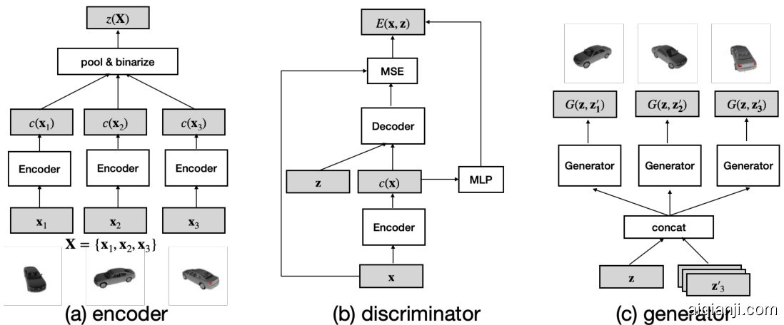
Figure 1: Model architectures of SDNs. SDNs consist of three modules: (a) a set encoder that maps a set of images into a discrete code, with a shared convolutional encoder encoding each image followed by average pooling and disc ret iz ation; (b) a conditional disc rim in at or (energy) for each image that takes the form of an auto encoder (similar to [25]); (c) a conditional generator that generates images conditioned on a set code $\mathbf{z}$ .

图 1: SDN的模型架构。SDN包含三个模块：(a) 集合编码器，将图像集合映射为离散代码，通过共享卷积编码器编码每张图像后执行平均池化和离散化；(b) 每个图像的条件判别器（能量函数），采用自编码器形式（类似[25]）；(c) 基于集合代码$\mathbf{z}$生成图像的条件生成器。

$$
\begin{array}{r l}&{\mathcal{L}_ {\psi}=-\mathrm{E}_ {{\mathbf{z}^{\prime},\sim p_ {\psi}(\mathbf{z}^{\prime})}_ {i=1,\dots,n}}\log[e^{-|[\mathbf{z}(\mathbf{X}^{\prime};\boldsymbol{\theta})\odot\mathbf{z}]-|_ {1}}e^{-\sum_ {\mathbf{x}\in\mathbf{X}^{\prime}}E(\mathbf{x},\mathbf{z};\boldsymbol{\theta})\big)}]\big|_ {\mathbf{X}^{\prime}={G(\mathbf{z},\mathbf{z}^{\prime};\boldsymbol{\psi})}_ {i=1,\dots,n}}}\ &{\qquad=\mathrm{E}_ {{\mathbf{z}^{\prime},\sim p_ {\psi}(\mathbf{z}^{\prime})}_ {i=1,\dots,n}}[|[\boldsymbol{z}(\mathbf{X}^{\prime};\boldsymbol{\theta})\odot\mathbf{z}]-|_ {1}+\sum_ {\mathbf{x}\in\mathbf{X}^{\prime}}E(\mathbf{x},\mathbf{z};\boldsymbol{\theta})\big)\big|_ {\mathbf{X}^{\prime}={G(\mathbf{z},\mathbf{z}^{\prime};\boldsymbol{\psi})}_ {i=1,\dots,n}}.}\end{array}
$$

With $\psi$ fixed, we can optimize $\theta$ with a loss that combines $\mathcal{L}_ {0}(\theta)$ and $\mathcal{L}_ {1}(\theta,\psi)$ . As is common practice in GAN and deep EBM training [3, 9, 25], we apply a margin based loss on $E(\mathbf{x},\mathbf{z};\theta)$ . In particular, we have found that it’s beneficial to apply two separate margins on the two terms of $E$ , this leads to the loss function of $\theta$ update as:

固定 $\psi$ 后，我们可以通过结合 $\mathcal{L}_ {0}(\theta)$ 和 $\mathcal{L}_ {1}(\theta,\psi)$ 的损失函数来优化 $\theta$。遵循GAN和深度EBM训练的常见做法 [3, 9, 25]，我们对 $E(\mathbf{x},\mathbf{z};\theta)$ 应用基于间隔的损失函数。具体而言，我们发现对 $E$ 的两项分别应用独立间隔能带来更好效果，因此 $\theta$ 更新的损失函数定义为：

$$
\begin{array}{r l}&{\mathcal{L}_ {\theta}=-\log\bar{p}_ {\theta}\big(\Omega\big(z\big(\mathbf{X};\theta\big)\big)\big)}\ &{\qquad+\displaystyle\sum_ {\mathbf{x}\in\mathbf{X}}|\mathbf{x}-d\big(z\big(\mathbf{X};\theta\big),c(\mathbf{x};\theta);\theta\big)|_ {2}^{2}+\big[\gamma_ {0}+d_ {0}(\mathbf{x};\theta)\big]_ {+}}\ &{\qquad+\operatorname{E}_ {\mathbf{X}^{\prime}\sim p_ {\psi}(\mathbf{X}|z(\mathbf{X}))}\displaystyle\sum_ {\mathbf{x}\in\mathbf{X}^{\prime}}\big[\gamma_ {1}-|\mathbf{x}-d\big(z(\mathbf{X};\theta),c(\mathbf{x};\theta);\theta\big)|_ {2}^{2}\big]_ {+}+\big[\gamma_ {0}-d_ {0}(\mathbf{x};\theta)\big]_ {+}.}\end{array}
$$

Here $\Omega$ is the stop gradient operator, indicating that we do not pass gradient from the prior to the encoder. $[\cdot]_ {+}$ is the operator that zeros out the negative portions of the input. $\gamma_ {0},\gamma_ {1}\in R^{+}$ are two margin parameters.

这里 $\Omega$ 是停止梯度算子，表示我们不将梯度从先验传递到编码器。$[\cdot]_ {+}$ 是将输入负值部分置零的算子。$\gamma_ {0},\gamma_ {1}\in R^{+}$ 是两个边界参数。

3 相关工作

Generative Modeling of sets. Generative modeling of sets is a challenging task. Hierarchical Bayes models have previously been widely applied to document modeling, which can be considered as a set of words, represented by the LDA model [2]. Recently, there has been a a body of work dedicated to point cloud generative modeling, where sets are composed of 3D points in Euclidean space [1, 13, 20]. However, image sets considered in our work contain much richer structure than 3D points. It is thus unclear how methods developed from the point cloud or document modeling lines of work generalize to more complex image data.

集合的生成式建模 (Generative Modeling)。集合的生成式建模是一项具有挑战性的任务。分层贝叶斯模型 (Hierarchical Bayes models) 此前已广泛应用于文档建模——文档可视为由LDA模型 [2] 表示的词集合。近期涌现了大量专注于点云生成建模的研究，这类集合由欧几里得空间中的3D点构成 [1, 13, 20]。然而，本文研究的图像集合比3D点具有更丰富的结构特征。因此，从点云或文档建模领域发展而来的方法如何泛化到更复杂的图像数据仍不明确。

Auto encoding GANs. SDNs are similar to a handful of existing works which involve an encoder, generator/decoder and a disc rim in at or [7, 8, 12]. Notably, BiGAN [7] trains a two channel discriminator that tries to separate the two joint distributions $p(\mathbf{z})p(\mathbf{x}|\mathbf{z})$ and $p(\mathbf{x})p(\mathbf{z}|\mathbf{x})$ . Aside from the set modeling aspect, in a BiGAN the encoder and decoder work jointly against the disc rim in at or, whereas in SDNs, the encoder and the disc rim in at or work jointly against the generator. Intuitively, SDNs encourage the encoder to learn disc rim i native representations by not allowing it to cooperate with the generator, which in turn improves the generator’s quality as well.

自编码生成对抗网络。SDN与少数现有工作类似，这些工作都包含编码器、生成器/解码器和判别器 [7, 8, 12]。值得注意的是，BiGAN [7] 训练了一个双通道判别器，试图区分两个联合分布 $p(\mathbf{z})p(\mathbf{x}|\mathbf{z})$ 和 $p(\mathbf{x})p(\mathbf{z}|\mathbf{x})$。除了集合建模方面，在BiGAN中编码器和解码器共同对抗判别器，而在SDN中，编码器和判别器共同对抗生成器。直观上，SDN通过禁止编码器与生成器合作，促使编码器学习判别性表征，这反过来也提高了生成器的质量。

Conditional GANs. A conditional GAN (cGAN) [15, 17] modifies the generator and disc rim in at or of a GAN to be conditional on class labels. SDNs can be considered a generalization of cGANs, as it learns the parametric set representation jointly with the generator and disc rim in at or.

条件GAN (Conditional GAN)。条件GAN (cGAN) [15, 17] 通过修改GAN的生成器和判别器，使其能够基于类别标签生成样本。SDN可视为cGAN的泛化形式，因为它能联合学习参数化集合表示与生成器及判别器。

VQ-VAEs. VQ-VAEs [18, 19] are related to SDNs in that they learn encoders that output discrete and deterministic codes. They also learn auto-regressive priors which greatly improves their capability of generative modeling. SDNs differ from VQ-VAEs in that they have a more sophisticated encoder and disc rim in at or, which are essential to cope with set structures.

VQ-VAEs。VQ-VAEs [18, 19] 与 SDNs 相关，因为它们学习的编码器输出离散且确定的代码。它们还学习自回归先验，这大大提高了生成建模的能力。SDNs 与 VQ-VAEs 的不同之处在于它们具有更复杂的编码器和判别器，这对于处理集合结构至关重要。

4 Experiments

4 实验

4.1 Datasets

4.1 数据集

The first dataset we use is ShapeNet [5], which consists of 3D objects with projected 2d views. We use a subset which contains 13 popular categories, namely airplane, bench, cabinet, car, chair, monitor, lamp, speaker, gun, couch, table, phone, ship. The training set consists of 32,837 unique objects and 788,088 images in total. The second dataset is VGGFace2 [4], which is a face dataset containing 9,131 subjects and 3.31M images.

我们使用的第一个数据集是ShapeNet [5]，它包含带有投影2D视图的3D对象。我们采用包含13个常见类别的子集：飞机、长椅、橱柜、汽车、椅子、显示器、台灯、音箱、枪支、沙发、餐桌、电话和轮船。训练集共包含32,837个独立对象和788,088张图像。第二个数据集VGGFace2 [4]是人脸数据集，涵盖9,131个主体和331万张图像。

For both datasets, we randomly construct fixed-size sets of 8 elements for training. For ShapeNet, this is done by randomly selecting an object and 8 of its views; for VGGFace2, we similarly select one identity and 8 of her/his faces. A mini-batch is constructed by selecting $N$ objects/subjects, which amounts to $N\times8$ images in total. All images are scaled to a size of $128\times128$ .

对于这两个数据集，我们随机构建固定大小为8元素的集合用于训练。在ShapeNet中，通过随机选择一个物体及其8个视角实现；在VGGFace2中，则随机选取一个身份及其8张人脸图像。每个小批量(mini-batch)通过选择$N$个物体/主体构成，共计$N\times8$张图像。所有图像统一缩放至$128\times128$分辨率。

4.2 Implementation Details

4.2 实现细节

Our implementation resembles that of SAGAN [23] w.r.t. base architecture and learning scheduling. The encoder is identical to the disc rim in at or in SAGAN, namely a CNN enhanced with Spectral Normalization (SN) [16] and Self Attention (SA), except that the number of output units is changed to $d_ {z}$ instead of 1. The dimension of $\mathbf{z}$ is 2048 and 256 for ShapeNet and VGGFace2, respectively. The generator is also the same as that in SAGAN, which is a CNN with SN, Batch Norm [11] and SA. The decoder for the disc rim in at or resembles the generator, but without BN and SA; the MLP for the unary energy term is a simple two layer ReLU neural network with $d_ {z}$ hidden units. All images are normalized to range $[-1,1]$ . We set the two margin parameters as $\gamma_ {0}=1,\gamma_ {1}=0.1,$ , which we have found to work robustly across various settings.

我们的实现方案在基础架构和学习调度方面与SAGAN [23]类似。编码器结构与SAGAN中的判别器(discriminator)相同，即采用谱归一化(Spectral Normalization, SN) [16]和自注意力机制(Self Attention, SA)增强的CNN网络，仅将输出单元数改为$d_ {z}$而非1。$\mathbf{z}$的维度在ShapeNet和VGGFace2数据集上分别为2048和256。生成器同样沿用SAGAN的架构，是由SN、批归一化(Batch Norm) [11]和SA构成的CNN网络。判别器解码器结构类似生成器，但移除了BN和SA模块；单点能量项的MLP是一个简单的双层ReLU神经网络，隐藏单元数为$d_ {z}$。所有图像归一化至$[-1,1]$范围。我们将两个边界参数设为$\gamma_ {0}=1,\gamma_ {1}=0.1$，该设置在各类实验环境中均表现稳健。

During training, we use Adam with a learning rate 1e-4 for the generator , and learning rate 4e-4 for the encoder, disc rim in at or, and prior. The momentum terms are set as ${0,0.999}$ for both optimizers. We use a batch size of 32 (consisting of 256 images), spread across 4 V100 GPUs. We alternatively update $\psi$ and $\theta$ one step per mini-batch, and train the models for approximately 600K iterations, which takes roughly two weeks.

训练过程中，我们为生成器 (generator) 使用学习率 1e-4 的 Adam 优化器，为编码器 (encoder)、判别器 (discriminator) 和先验网络 (prior) 使用学习率 4e-4。两个优化器的动量项均设为 ${0,0.999}$。批处理大小为 32（包含 256 张图像），分布在 4 块 V100 GPU 上。我们交替更新 $\psi$ 和 $\theta$，每个小批次执行一步更新，模型训练约 60 万次迭代，耗时约两周。

4.3 Qualitative Results

4.3 定性结果

By construction, SDNs are able to reconstruct (stochastic ally) an input set, and generate new sets by sampling from the prior. We show example inputs, reconstructions and samples in Fig. 2, 4, 6, 7. We see that SDNs produce semantically meaningful, consistent reconstructions of unseen input sets. The samples from the prior are also coherent. For faces, the SDN captures variations in hairstyle, expression, and pose, while retaining gender and ethnicity of the input identities. For ShapeNet, we

通过设计，SDN能够（随机地）重建输入集，并通过从先验中采样生成新集合。我们在图2、4、6、7中展示了输入示例、重建结果和采样样本。可见SDN能对未见过的输入集生成语义明确、逻辑一致的重建结果，其先验采样样本同样具有连贯性。对于人脸数据，SDN能捕捉发型、表情和姿态的变化，同时保留输入个体的性别与种族特征。对于ShapeNet数据集，我们...

Figure 2: Top: example set from the test split of ShapeNet; bottom: reconstructed set. There is no correspondence between images from the two sets.

图 2: 上: ShapeNet测试集的示例集合；下: 重建集合。两组图像之间不存在对应关系。

Figure 3: (a) Input, and (b) reconstructed sets from a ShapeNet car where samples are arranged on a circle by manually estimated pose (see Supp. Material for details.) This visualization shows consistency in terms of appearance and pose variability between input and reconstructed sets.

图 3: (a) 输入, 以及 (b) 从ShapeNet汽车数据集重建的集合, 其中样本通过手动估计的位姿沿圆形排列(详见补充材料)。该可视化展示了输入集与重建集在外观和位姿变化方面的一致性。

show in Fig. 3 that the reconstructed sets match their input counterparts in terms of object consistency and pose diversity. See Supp. Materials for more qualitative results.

图 3 显示重建集合在物体一致性和姿态多样性方面与输入对应物相匹配。更多定性结果见补充材料。

4.4 ShapeNet Evaluations

4.4 ShapeNet评估

In order to show that ShapeNet sets reconstructed by SDNs are consistent quantitatively, we take a pre-trained Occupancy Network [14] (OccNet) and use it to generate 3D meshes from images of both real and SDN-reconstructed sets, where SDNs and OccNets are trained on the same train/test splits and rendered views. We extend OccNets [14] to deal with multiple views by a simple average pooling of its encoder output across views, and refer readers to [14] and the Supp. Material for more details.

为了定量展示SDN重建的ShapeNet数据集具有一致性，我们采用预训练的Occupancy Network [14] (OccNet) 从真实图像和SDN重建图像生成3D网格。SDN与OccNet使用相同的训练/测试集划分及渲染视角进行训练。我们通过多视角编码器输出的简单平均池化扩展了OccNets [14] 的多视角处理能力，更多细节详见[14]及补充材料。

We empirically evaluate SDNs by computing Chamfer Distance2 (CD) [1] and IoU as in [14] between corresponding 3D meshes obtained from real and SDN-reconstructed sets. We denote these meshes as $\mathcal{M}$ and $\hat{\mathcal{M}}$ , respectively. We compute the CD on 2048 points sampled from the surface of each mesh. To approximate the IoU we sample 2048 points on the volume of each mesh and compute the average proportion of points of $\mathcal{M}$ contained in the volume of $\hat{\mathcal{M}}$ and vice-versa. We expect that if SDN-reconstructed sets represent accurate and consistent views of the same object, both metrics will improve as the difference between reconstructed and real sets decreases.

我们通过计算真实三维网格与SDN重建网格间的倒角距离(Chamfer Distance2, CD) [1] 和交并比(IoU) [14] 进行实证评估，分别记为 $\mathcal{M}$ 和 $\hat{\mathcal{M}}$。CD计算基于每个网格表面采样的2048个点。为估算IoU，我们在每个网格体积内采样2048个点，计算 $\mathcal{M}$ 的点在 $\hat{\mathcal{M}}$ 体积内的平均占比（反之亦然）。若SDN重建集能准确一致地反映同一物体，随着重建集与真实集差异减小，两项指标应同步提升。

2We report $\mathrm{{CD}\times10^{3}}$

2我们报告 $\mathrm{{CD}\times10^{3}}$

Figure 4: Two sets sampled from the prior on ShapeNet.

图 4: 从ShapeNet先验分布中采样的两组样本。

Figure 5: Left: real set and 3D reconstruction. Right: reconstructed set and 3D reconstruction. For this example the IoU and CD are 0.784 and 4.289, respectively.

图 5: 左图: 真实集与三维重建。右图: 重建集与三维重建。该示例的交并比 (IoU) 和倒角距离 (CD) 分别为 0.784 和 4.289。

Figure 6: Top: an example set from the test split of VggFace2; bottom: the reconstructed set. There is no correspondence between images from the two sets.

图 6: 上: VggFace2测试集的一个示例集合；下: 重建后的集合。两组图像之间不存在对应关系。

We verify this hypothesis with two experiments, both conducted on the test split of ShapeNet. In the first experiment we fix the size of real sets to 16 views and vary the number of views sampled from the reconstructed set3. We then use the sets to compute meshes $\mathcal{M}$ and $\hat{\mathcal{M}}$ . We see that as the number of sampled reconstructed views increases, we consistently get better reconstructions, as shown in Tab. 1 (a).

我们通过两个实验验证这一假设，均在ShapeNet的测试集上进行。第一个实验中，我们将真实视图集大小固定为16张，并改变从重建集中采样的视图数量[3]，随后利用这些视图集计算网格$\mathcal{M}$和$\hat{\mathcal{M}}$。如表1(a)所示，随着采样重建视图数量的增加，重建质量持续提升。

#Recon.views	1	4	8	16	#Input views	1	4	8	16
CD←	4.458	3.682	3.501	3.433	CD ↓	6.333	3.912	3.590	3.434
IoU↑	0.679	0.711	0.719	0.722	IoU↑	0.633	0.701 (b)	0.715	0.722
(a)

#重建视图	1	4	8	16	#输入视图	1	4	8	16
CD←	4.458	3.682	3.501	3.433	CD↓	6.333	3.912	3.590	3.434
IoU↑	0.679	0.711	0.719	0.722	IoU↑	0.633	0.701 (b)	0.715	0.722
(a)

Table 1: (a) 3D reconstruction results as a function of the reconstructed set size. (b) 3D reconstruction results as a function of the number of samples $n$ used in the compute the set code $z(\mathbf{X})$ .

表 1: (a) 三维重建结果随重建集大小的变化关系。(b) 三维重建结果随用于计算集编码 $z(\mathbf{X})$ 的样本数 $n$ 的变化关系。

For our second experiment we vary the number of input views used to compute the set code $z(\mathbf{X})$ , while keeping the number of reconstructed views constant (16). We compute the reconstructed meshes and compare them with the corresponding mesh obtained with all 16 input views. Our hypothesis is that the set representation gets better as the number of samples in $\mathbf{X}$ increases, and therefore sets can be more accurately reconstructed, which will lead to better 3D reconstructions, as shown in Tab. 1(b). Finally, in Fig. 5 we show qualitative comparisons of 3D meshes obtained from real vs. reconstructed sets, where both contain 16 elements.

在我们的第二个实验中，我们改变了用于计算集合编码 $z(\mathbf{X})$ 的输入视图数量，同时保持重建视图数量恒定(16)。我们计算重建网格，并将其与使用全部16个输入视图获得的对应网格进行比较。我们的假设是：随着 $\mathbf{X}$ 中样本数量的增加，集合表示会变得更优，因此可以更准确地重建集合，这将带来更好的3D重建效果，如表1(b) 所示。最后，在图5中我们展示了从真实集合与重建集合(均包含16个元素)获得的3D网格的定性对比结果。

4.5 VGGFace2 Evaluations

4.5 VGGFace2 评估

To provide quantitative results of set reconstruction performance for faces, we examine identity verification ROC curves on the VGGFace2 dataset using a pre-trained face verification model from [4]. We evaluate both reconstructed samples and samples generated from the prior, corresponding to Fig. 6 and Fig. 7, respectively. All input sets are taken from the test split of VGGFace2.

为了量化评估人脸集合重建的性能表现，我们在VGGFace2数据集上采用[4]提出的预训练人脸验证模型，绘制了身份验证ROC曲线。实验同时评估了重建样本与先验分布生成样本（分别对应图6和图7），所有输入集合均取自VGGFace2测试集。

Figure 7: Two sets sampled from the prior on VGGFace2.

图 7: 从VGGFace2先验分布中采样的两组样本。

Figure 8: Identity verification performance with a pre-trained VGGFace2 model. ’recon and real’: matching reconstructed images to real images; ’real’: matching real images; ’recon’: matching reconstructed images; ’free samples’: matching samples generated from the learned prior. ’uniform samples’: matching samples generated from a uniform prior.

图 8: 使用预训练 VGGFace2 模型的身份验证性能。'recon and real': 将重建图像与真实图像匹配; 'real': 真实图像匹配; 'recon': 重建图像匹配; 'free samples': 与从学习先验生成的样本匹配; 'uniform samples': 与从均匀先验生成的样本匹配。

As a preprocessing step, we convert each image (real and generated) into a fixed dimensional embedding with the VGGFace2 model. We then use the distances in the embedding space to compare same and different identities’ true-positive rate (TPR) and false-positive rate (FPR). We plot the ROC curve for different types of input images in Figure 8a. We see that the curve for reconstructed images (’recon’) is close to that of real images (’real’), suggesting that the reconstructed sets are diverse and also that the images within a set are consistent with each other. Comparing the reconstruction to real images (’recon and real’), we see that the reconstructions are diverse and self-consistent, although the SDN does not strictly preserve identity in the reconstructed sets. As a better calibration of this difference, we also show the ROC for real images with different proportions of label noise in Figure 8c. Here we randomly contaminate the sets of real images with increasing numbers of images from different identities. We can see that the reconstruction performance at different FPR thresholds approximates different levels of label noise. For example, at a $10%$ FPR, we see that the reconstruction sets perform similarly to real identities with $25%$ label noise.

作为预处理步骤，我们使用VGGFace2模型将每张图像（真实和生成的）转换为固定维度的嵌入向量。随后通过嵌入空间中的距离来比较相同与不同身份的真阳性率（TPR）和假阳性率（FPR）。图8a展示了不同类型输入图像的ROC曲线。可以看到重建图像（'recon'）的曲线与真实图像（'real'）接近，表明重建集具有多样性且组内图像相互一致。将重建图像与真实图像（'recon and real'）对比时，尽管SDN未严格保持重建集中的身份特征，但其重建结果仍展现出多样性和自洽性。为量化这种差异，图8c展示了添加不同比例标签噪声的真实图像ROC曲线——我们通过随机混入递增数量的异身份图像来污染真实图像集。结果显示，不同FPR阈值下的重建性能近似于不同级别的标签噪声。例如在10% FPR时，重建集的表现相当于含有25%标签噪声的真实身份数据集。

Additionally, we look at the effect of context size on the reconstructed images in Figure 8b. Even though the SDN was trained with a constant context size of 8, increasing the size of the input set improves the performance, and here we see reconstructed images approach even closer the performance of the model on the real images, which is also consistent with Table 1.

此外，我们在图 8b 中研究了上下文大小对重建图像的影响。尽管 SDN 训练时使用的上下文大小固定为 8，但增大输入集规模能提升性能。此处可见重建图像进一步接近模型在真实图像上的表现，这也与表 1 的结果一致。

5 Conclusion

5 结论

In this paper, we presented SDNs, a novel probabilistic generative model for image sets. We demonstrated that SDNs can be successfully trained on two real world datasets, ShapeNet and VGGFace2, at $128\times128$ resolution. We proposed to evaluate trained SDNs with a pretrained 3D reconstruction network and a face verification network, respectively, and showed that the trained SDNs generate high quality image sets both qualitatively and quantitatively.

本文提出了一种新颖的图像集概率生成模型SDN。我们证明了SDN能在128×128分辨率下成功训练两个真实世界数据集(ShapeNet和VGGFace2)。通过分别采用预训练的3D重建网络和人脸验证网络评估训练后的SDN，结果表明该模型在定性和定量层面均能生成高质量图像集。

Appendix

附录

A More samples

B Varying input set size

B 不同输入集大小

SDNs are trained with fixed set sizes (8 in our experiments). But because of the use of average pooling in the encoder, it is possible to test a trained SDN with varied input sizes (Table 1(b) in main text). We show four such results in Fig. 13. we see that an SDN is able to effectively utilize more input samples within the set and produce in re a singly more consistent reconstructions.

SDN在训练时使用固定集合大小(实验中为8)。但由于编码器中采用了平均池化，可以在测试时输入不同大小的集合(主文中的表1(b))。我们在图13中展示了四个此类结果，可见SDN能够有效利用集合中更多的输入样本，从而生成更加一致的重建结果。

C 3D reconstruction on ShapeNet

基于ShapeNet的3D重建

Our 3D reconstruction experiments show that SDN-reconstructed sets are accurate and consistent. In this section, we describe in more detail our extension of Occupancy Networks [14] to deal with multiple input RGB views, which is not discussed in [14]. Occupancy Networks use a convolutional encoder to compute a $d$ -dimensional latent representation $\mathbf{c}\in\mathbb{R}^{d}$ for a given RGB view. This latent representation is then used as conditioning for an MLP $f_{\theta}^{\star} \colon \mathbb{R}^{3}×\mathbb{R}^{d} \to \mathbb{R}$ that takes 3D points and predicts their occupancy (ie. whether the points lie inside or outside the object mesh).

我们的3D重建实验表明，SDN重建结果准确且一致。本节将详细描述我们对Occupancy Networks [14] 的扩展，以处理多输入RGB视图（该问题在[14]中未讨论）。Occupancy Networks使用卷积编码器计算给定RGB视图的$d$维潜在表征$\mathbf{c}\in\mathbb{R}^{d}$，该潜在表征随后作为MLP $f_ {\theta}^{\star}\colon{\mathbb{R}}^{3}×{\mathbb{R}}^{d}\to{\mathbb{R}}$的条件输入，该MLP接收3D点并预测其占用情况（即判断点位于物体网格内部或外部）。

Our hypothesis is that by average pooling the latent representations c obtained by each element on a set (remember each element on a set corresponds to a different viewpoint of the same object) we can increase the amount of information about the object contained in c. However, that is only true if the latent representations c of different views are in agreement, in other words, if they are different views of the same object. To check this assumption we take a pre-trained Occupancy Network trained on single views (check [14] for more details) and show in Tab. 2 that reconstruction accuracy as measured by IoU increases when the latent representations c are pooled across views of the same object4. These results show that if elements of a SDN-reconstructed set are in agreement (eg. if a set contains different viewpoints of the same underlying object) reconstruction accuracy should improve when average pooling across elements in the set.

我们的假设是，通过对集合中每个元素获得的潜在表征c进行平均池化（记住集合中的每个元素对应同一对象的不同视角），可以增加c中包含的关于对象的信息量。然而，只有当不同视角的潜在表征c保持一致时（即它们属于同一对象的不同视角），这一假设才成立。为验证该假设，我们采用了一个预训练的单视角Occupancy Network（详见[14]），并在表2中展示了当潜在表征c在同一对象的多视角间进行池化时，IoU测量的重建精度有所提升。这些结果表明：若SDN重建集合中的元素具有一致性（例如集合包含同一底层对象的不同视角），则对集合元素进行平均池化时应能提高重建精度。

	↑IoU
	1 view	5views
Mean	0.593	0.621

| | ↑IoU |
| | 1 view | 5views |
| Mean | 0.593 | 0.621 |

Table 2: Aggregating multiple views for Occupancy Networks improves reconstruction accuracy.

表 2: 多视角聚合可提升Occupancy Networks的重建精度。

In Fig. 14 we show uncurated pairs of real and SDN-reconstructed sets together with their respective 3D reconstructions obtained by running our Occupancy Networks extension. For each grid the two first rows correspond to real set and an orbit of its predicted 3D reconstruction and the two last rows correspond to SDN-reconstructed set and its corresponding 3D reconstruction.

在图14中，我们展示了未经筛选的真实集合与SDN重建集合的对比组，以及通过运行Occupancy Networks扩展获得的各自3D重建结果。每个网格的前两行对应真实集合及其预测3D重建的轨迹，后两行对应SDN重建集合及其相应的3D重建。

Finally, Fig. 15 shows sets sampled from the SDN prior and their corresponding 3D reconstruction. For each grid in the top row we show the sampled sets of 8 elements from the prior, and the bottom two rows show and orbit of the 3D mesh.

最后，图 15 展示了从 SDN 先验中采样的集合及其对应的 3D 重建结果。顶行每个网格中展示了从先验中采样的 8 元素集合，底部两行则展示了 3D 网格的轨迹。

Figure 9: More reconstructions of objects from the test split ShapeNet. For each block the top row is the input set and the bottom row is the reconstructed set.

图 9: ShapeNet测试集部分物体的更多重建结果。每个区块的顶行为输入点集，底行为重建点集。

Figure 10: More reconstructions of objects from the test split VggFace2. For each block the top row is the input set and the bottom row is the reconstructed set.

图 10: VggFace2测试集部分物体的更多重建结果。每个区块的顶部行是输入集，底部行是重建集。

Figure 11: Uncurated ShapeNet samples from the learned auto regressive prior (left) and a uniform prior (right).

图 11: 从学习的自回归先验 (左) 和均匀先验 (右) 中未经筛选的 ShapeNet 样本。

D Qualitative Analysis of Within Set Variation

D 组内变异的定性分析

In this section, we visualize the consistency and diversity of samples within a set produced by our SDN trained on ShapeNet object instances. To do so, for several object instances, we manually order samples by their pose (as estimated by a human annotator) to generate a continuum. We then map this continuum to a circle representing how the pose varies along the viewing sphere. By visualizing the input and reconstructed sets in this way we can examine how well the reconstructions capture the pose variability of the inputs. The reconstructions qualitatively capture the appearance of the input set (consistency) and the pose variation around the circle (diversity), with no sign of mode collapse. For the input set, we sampled 16 images randomly for that object. For the reconstructed set, we sampled 64 images, ordered them manually by visual inspection, and then decimated the continuum to obtain 16 reconstruction images.

在本节中，我们可视化由基于ShapeNet物体实例训练的SDN生成样本集的一致性和多样性。为此，我们针对若干物体实例，通过人工标注者估计的姿态对样本进行手动排序以生成连续序列，并将该序列映射至代表视角球面姿态变化的圆形轨迹上。通过这种输入集与重建集的可视化对比，可以评估重建结果对输入姿态变化的捕捉能力。重建结果在定性层面同时保留了输入集的表观特征（一致性）和圆形轨迹上的姿态变化（多样性），且未出现模式坍塌迹象。输入集采用随机采样16张物体图像，重建集则采样64张图像后经人工视觉排序，并通过降采样获得16张重建图像。

Figure 12: Uncurated VGGFace2 samples from the learned auto regressive prior (left) and a uniform prior (right).

图 12: 从学习的自回归先验 (左) 和均匀先验 (右) 中采样的未筛选 VGGFace2 样本。

Figure 13: Reconstructions by varying input set size (see Table 1(b) in main text). For each block, the top row is the input set, with the following rows showing reconstructions obtained with the first, first 4 and all 8 views, respectively.

图 13: 不同输入集大小的重建效果 (参见正文表 1(b) )。每个区块的顶行为输入集，后续行分别展示使用第1个、前4个和全部8个视角获得的重建结果。

Figure 14: Random sampling of real and SDN-reconstructed sets with their corresponding 3D reconstructions obtained by our Occupancy Network extension. Each block shows an input views, input 3D meshes, reconstructed views, reconstructed 3D meshes, from top to bottom.

图 14: 真实样本与SDN重建样本的随机采样对比及其通过Occupancy Network扩展获得的对应三维重建结果。每个区块从上至下依次展示：输入视图、输入三维网格、重建视图、重建三维网格。

Figure 15: Sets sampled from the SDN prior with their corresponding 3D reconstruction. Each block shows a generated set consisting of 8 views and 16 of its reconstructed 3D mesh projections.

图 15: 从SDN先验中采样的集合及其对应的3D重建。每个区块展示了一个生成的集合，包含8个视角和16个重建的3D网格投影。

Figure 16: Input (a) and reconstructed (b) sets from a ShapeNet bench where samples are arranged on a circle by manually estimated pose (see Supplementary Material for details). This visualization shows consistency in terms of appearance and pose variability between input and reconstructed sets.

图 16: 输入集 (a) 与重建集 (b) 来自ShapeNet长凳数据集，其中样本通过手动估计的姿态沿圆形排列 (详见补充材料)。该可视化展示了输入集与重建集在外观和姿态变化方面的一致性。

[论文翻译]集合分布网络：一种面向图像集合的生成模型

原文地址：https://arxiv.org/pdf/2006.10705v1

Set Distribution Networks: a Generative Model for Sets of Images

集合分布网络：一种面向图像集合的生成模型

Abstract

1 Introduction

1 引言

2 Methodology

2 方法论

2.1 Set Distribution Networks

2.1 集合分布网络

2.2 Approximate Inference with Learned Prior and Generator

2.2 基于学习先验和生成器的近似推断

2.3 Model Architectures

2.4 Losses

2.4 损失函数

3 相关工作

4 Experiments

4 实验

4.1 Datasets

4.1 数据集

4.2 Implementation Details

4.2 实现细节

4.3 Qualitative Results

4.4 ShapeNet Evaluations

4.4 ShapeNet评估

4.5 VGGFace2 Evaluations

4.5 VGGFace2 评估

5 Conclusion

5 结论

Appendix

A More samples

更多样本

B Varying input set size

B 不同输入集大小

C 3D reconstruction on ShapeNet

基于ShapeNet的3D重建

D Qualitative Analysis of Within Set Variation

D 组内变异的定性分析

[论文翻译]集合分布网络：一种面向图像集合的生成模型

原文地址：https://arxiv.org/pdf/2006.10705v1

Set Distribution Networks: a Generative Model for Sets of Images

集合分布网络：一种面向图像集合的生成模型

Abstract

1 Introduction

1 引言

2 Methodology

2 方法论

2.1 Set Distribution Networks

2.1 集合分布网络

2.2 Approximate Inference with Learned Prior and Generator

2.2 基于学习先验和生成器的近似推断

2.3 Model Architectures

2.4 Losses

2.4 损失函数

3 Related Work

3 相关工作

4 Experiments

4 实验

4.1 Datasets

4.1 数据集

4.2 Implementation Details

4.2 实现细节

4.3 Qualitative Results

4.4 ShapeNet Evaluations

4.4 ShapeNet评估

4.5 VGGFace2 Evaluations

4.5 VGGFace2 评估

5 Conclusion

5 结论

Appendix

A More samples

更多样本

B Varying input set size

B 不同输入集大小

C 3D reconstruction on ShapeNet

基于ShapeNet的3D重建

D Qualitative Analysis of Within Set Variation

D 组内变异的定性分析