Synthetic Petri Dish: A Novel Surrogate Model for Rapid Architecture Search
Synthetic Petri Dish: 一种用于快速架构搜索的新型代理模型
Aditya Rawal 1 Joel Lehman 1 Felipe Petroski Such 1 Jeff Clune* 2 Kenneth O. Stanley* 1
Aditya Rawal 1 Joel Lehman 1 Felipe Petroski Such 1 Jeff Clune* 2 Kenneth O. Stanley* 1
Abstract
摘要
Neural Architecture Search (NAS) explores a large space of architectural motifs – a computeintensive process that often involves ground-truth evaluation of each motif by instant i a ting it within a large network, and training and evaluating the network with thousands or more data samples. Inspired by how biological motifs such as cells are sometimes extracted from their natural environment and studied in an artificial Petri dish setting, this paper proposes the Synthetic Petri Dish model for evaluating architectural motifs. In the Synthetic Petri Dish, architectural motifs are instantiated in very small networks and evaluated using very few learned synthetic data samples (to effectively approximate performance in the full problem). The relative performance of motifs in the Synthetic Petri Dish can substitute for their ground-truth performance, thus accelerating the most expensive step of NAS. Unlike other neural network-based prediction models that parse the structure of the motif to estimate its performance, the Synthetic Petri Dish predicts motif performance by training the actual motif in an artificial setting, thus deriving predictions from its true intrinsic properties. Experiments in this paper demonstrate that the Synthetic Petri Dish can therefore predict the performance of new motifs with significantly higher accuracy, especially when insufficient ground truth data is available. Our hope is that this work can inspire a new research direction in studying the performance of extracted components of models in a synthetic diagnostic setting optimized to provide informative evaluations.
神经架构搜索(NAS)通过实例化大型网络对各类架构单元进行真实评估,需要消耗大量计算资源进行架构单元空间的探索。受生物学研究中将细胞等单元从自然环境中提取并在人工培养皿中观察的启发,本文提出用于评估架构单元的合成培养皿模型。在该模型中,架构单元被实例化为微型网络,仅需极少量合成数据样本即可有效预测其在完整任务中的性能表现。合成培养皿中的相对性能可替代真实性能评估,从而加速NAS中最耗时的环节。与基于神经网络解析单元结构来预测性能的方法不同,合成培养皿通过在实际人工环境中训练目标单元来预测性能,因此能根据其本质特性获得更准确的预测。实验表明,该方法对新架构单元的性能预测精度显著提升,尤其在真实训练数据不足时优势更为明显。本研究有望开创通过优化合成诊断环境来评估模型组件性能的新研究方向。
1. Introduction
1. 引言
The architecture of deep neural networks (NNs) is critical to their performance. This fact motivates neural architecture search (NAS), wherein the choice of architecture is often framed as an automated search for effective motifs, i.e. the design of a repeating recurrent cell or activation function that is repeated often in a larger NN blueprint. However, evaluating a candidate architecture’s ground-truth performance in a task of interest depends upon training the architecture to convergence. Complicating efficient search, the performance of an architectural motif nearly always benefits from increased computation (i.e. larger NNs trained with more data). The implication is that the best architectures often require training near the bounds of what computational resources are available, rendering naive NAS (i.e. where each candidate architecture is trained to convergence) exorbitantly expensive.
深度神经网络 (NN) 的架构对其性能至关重要。这一事实推动了神经架构搜索 (NAS) 的发展,其中架构选择通常被定义为对有效基元 (motif) 的自动化搜索,即在更大的神经网络蓝图中重复出现的循环单元或激活函数的设计。然而,评估候选架构在目标任务中的真实性能,需要将其训练至收敛状态。由于架构基元的性能几乎总是受益于计算量的增加 (即用更多数据训练更大的神经网络),这使得高效搜索变得更加复杂。这意味着最佳架构通常需要在可用计算资源的极限范围内进行训练,导致朴素 NAS (即每个候选架构都训练至收敛) 的成本极其高昂。
To reduce the cost of NAS, methods often exploit heuristic surrogates of true performance. For example, motif performance can be evaluated after a few epochs of training or with scaled-down architectural blueprints, which is often still expensive (because maintaining reasonable fidelity between ground-truth and surrogate performance precludes aggressive scaling-down of training). Another approach learns models of the search space (e.g. Gaussian processes models used within Bayesian optimization), which improve as more ground-truth models are trained, but cannot generalize well beyond the examples seen. This paper explores whether the computational efficiency of NAS can be improved by creating a new kind of surrogate, one that can benefit from miniaturized training and still generalize beyond the observed distribution of ground-truth evaluations. To do so, we take inspiration from an idea in biology, bringing to machine learning the application of a Synthetic Petri Dish microcosm that aims to identify high-performing archit ect ural motifs.
为降低神经架构搜索(NAS)成本,常见方法采用真实性能的启发式替代指标。例如,可通过少量训练周期评估架构单元性能,或使用缩微版架构方案(但这种方法仍代价高昂,因为要维持基准性能与替代指标间的合理保真度,就无法过度压缩训练规模)。另一种方案是学习搜索空间的模型(如贝叶斯优化中的高斯过程模型),其性能随基准模型训练量增加而提升,但难以泛化到未见过的样本。本文探索能否通过新型替代指标提升NAS计算效率——这种指标既能受益于微型化训练,又可泛化至超出基准评估的观测分布。为此,我们从生物学概念中获得启发,将"合成培养皿微宇宙"应用于机器学习,旨在识别高性能架构单元。
The overall motivation behind “in vitro” (test-tube) experiments in biology is to investigate in a simpler and controlled environment the key factors that explain a phenomenon of interest in a messier and more complex system. For example, to understand causes of atypical mental development, scientists extract individual neuronal cells taken from brains of those demonstrating typical and atypical behavior and study them in a Petri dish (Adhya et al., 2018). The approach proposed in this paper attempts to algorithmic ally recreate this kind of scientific process for the purpose of finding better neural network motifs. The main insight is that biological Petri dish experiments often leverage both (1) key aspects of a system’s dynamics (e.g. the behavior of a single cell taken from a larger organism) and (2) a humandesigned intervention (e.g. a measure of a test imposed on the test-tube). In an analogy to NAS, (1) the dynamics of learning through back propagation are likely important to understanding the potential of a new architectural motif, and (2) compact synthetic datasets can illuminate an architecture’s response to learning. That is, we can use machine learning to learn data such that training an architectural motif on the learned data results in performance indicative of the motif’s ground-truth performance.
生物学中"体外"(试管)实验的核心动机,是通过更简单可控的环境研究关键因素,从而解释更复杂混沌系统中的目标现象。例如为理解非典型心智发育成因,科学家会从典型和非典型行为者大脑中提取单个神经元细胞,在培养皿中进行研究 (Adhya et al., 2018)。本文提出的方法尝试用算法复现这类科学流程,以发现更优的神经网络模块。核心洞见在于:生物培养皿实验往往同时利用(1) 系统动态的关键特征(如从大型生物体提取的单个细胞行为),以及(2) 人为设计的干预措施(如对试管实施的测试方法)。类比神经架构搜索(NAS):(1) 通过反向传播的学习动态对理解新架构模块潜力至关重要,(2) 紧凑的合成数据集能揭示架构对学习的响应特性。换言之,我们可以用机器学习生成特定数据,使得在生成数据上训练架构模块的表现能反映其真实性能潜力。
In the proposed approach, motifs are extracted from their ground-truth evaluation setting (i.e. from large-scale NNs trained on the full dataset of the underlying domain of interest, e.g. MNIST), instantiated into very small networks (called motif-networks), and evaluated on learned synthetic data samples. These synthetic data samples are trained such that the performance ordering of motifs in this Petri dish setting (i.e. a miniaturized network trained on a few synthetic data samples) matches their ground-truth performance ordering. Because the relative performance of motifs is sufficient to distinguish good motifs from bad ones, the Petri dish evaluations of motifs can be a surrogate for ground-truth evaluations in NAS. Training the Synthetic Petri Dish is also computationally inexpensive, requiring only a few groundtruth evaluations, and once trained it enables extremely rapid evaluations of new motifs.
在所提出的方法中,从真实评估设置(即在目标领域完整数据集上训练的大规模神经网络,例如MNIST)中提取模体,实例化为极小型网络(称为模体网络),并在学习的合成数据样本上进行评估。这些合成数据样本经过训练,使得在这种培养皿设置(即在少量合成数据样本上训练的微型网络)中模体的性能排序与其真实性能排序相匹配。由于模体的相对性能足以区分优劣,培养皿评估可作为神经架构搜索中真实评估的替代方案。训练合成培养皿的计算成本也很低,仅需少量真实评估,一旦训练完成即可快速评估新模体。
A key motivating hypothesis is that because the Synthetic Petri Dish evaluates the motif by actually using it in a simple experiment (e.g. training it with SGD and then evaluating it), its predictions can generalize better than other neural network (NN) based models that predict motif performance based on only observing the motif’s structure and resulting performance (Liu et al., 2018a; Luo et al., 2018). For ex- ample, consider the demonstration problem of predicting the ground-truth performance of a two-layer feed forward MNIST network with sigmoidal non-linearity. The blue points in Figure 1 shows how the ground-truth performance of the MNIST network varies when the slope of its sigmoid activation s (the term $c$ in the sigmoid formula $1/(1+e^{-c x});$ is varied in the range of $0.01-2.01$ . The MNIST network performance peaks near a slope-value of 0.23. Similarly to the NN-based model previously developed in Liu et al. (2018a); Luo et al. (2018), one can try to train a neural network that predicts the performance of the corresponding MNIST network given the sigmoid slope value as input (Section 4.1 provides full details). When training points (tuples of sigmoid slope value and its corresponding MNIST network performance) are restricted to an area to the right of the peak (Figure 1, blue-shaded region), the NN-based prediction model (Figure 1, red diamonds) generalizes poorly to the test points on the left side of the peak $'c<0.23)$ . However, unlike such a conventional prediction model, the prediction of the Synthetic Petri Dish generalizes to test points left of the peak (despite their behavior being drastically different than what would be expected solely based on the points in the blue shaded region). That occurs because the Synthetic Petri Dish trains and evaluates the actual can- didate motifs, rather than just making predictions about their performance based on data from past trials.
一个关键驱动假设是,由于合成培养皿(Synthetic Petri Dish)通过在实际简单实验中使用基元来评估其性能(例如用SGD训练后评估),其预测结果比其他基于神经网络(NN)的模型更具泛化性——后者仅通过观察基元结构和历史表现来预测性能(Liu et al., 2018a; Luo et al., 2018)。例如在预测具有S型非线性的双层MNIST前馈网络真实性能的示例中,图1蓝点展示了当S型激活函数斜率s(sigmoid公式$1/(1+e^{-c x})$中的$c$项)在$0.01-2.01$范围内变化时,MNIST网络性能的变化情况,其峰值出现在斜率值0.23附近。与Liu et al. (2018a)和Luo et al. (2018)开发的NN模型类似,可以尝试训练一个以S型斜率值为输入的神经网络来预测对应MNIST网络性能(详见第4.1节)。当训练数据(S型斜率值与对应MNIST网络性能的元组)被限制在峰值右侧区域时(图1蓝色阴影区),基于NN的预测模型(图1红色菱形)对峰值左侧测试点($c<0.23$)的泛化表现较差。但与传统预测模型不同,合成培养皿的预测能够泛化至峰值左侧测试点(尽管这些点的表现与仅基于蓝色阴影区数据推导的预期截然不同)。这是因为合成培养皿会实际训练和评估候选基元,而非仅根据历史试验数据进行性能预测。
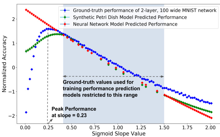
Figure 1. Predicting the Optimal Slope of the Sigmoid Activation. Each blue diamond depicts the normalized validation accu- racy (ground-truth) of a 2-layer, 100-wide feed-forward network with a unique sigmoid slope value (mean of 20 runs). The validation accuracy peaks at a slope of 0.23. Both the Synthetic Petri Dish and a neural network surrogate model that predicts performance as a function of sigmoid slope are trained on a limited set of ground-truth points (in total 15), restricted to the blue-shaded region to the right of the peak. The normalized performance predictions for Synthetic Petri Dish are shown with green diamonds and those for the NN surrogate model are shown as red diamonds. The plot shows that for test points on the left of the training data, the NN model is unable to infer that a peak exists with a dramatic falloff to the left of it. In contrast, because the Synthetic Petri Dish conducts experiments with small neural networks with these sigmoid slope values it is more more accurate at inferring both that there is a peak with a falloff to the left and its approximate location.
图 1: 预测Sigmoid激活函数的最佳斜率。每个蓝色菱形表示具有唯一Sigmoid斜率值的2层100宽度前馈网络的归一化验证准确率(真实值)(20次运行的平均值)。验证准确率在斜率为0.23时达到峰值。合成培养皿(Synthetic Petri Dish)和用于预测性能随Sigmoid斜率变化的神经网络代理模型均在有限的真实数据点(总计15个)上训练,这些数据点限制在峰值右侧的蓝色阴影区域。合成培养皿的归一化性能预测结果用绿色菱形表示,神经网络代理模型的预测结果用红色菱形表示。图表显示,对于训练数据左侧的测试点,神经网络模型无法推断出峰值的存在及其左侧的急剧下降。相比之下,由于合成培养皿使用具有这些Sigmoid斜率值的小型神经网络进行实验,因此在推断峰值存在、左侧下降及其大致位置方面更为准确。
Beyond this explanatory experiment, the promise of the Synthetic Petri Dish is further demonstrated on a challenging and compute-intensive language modelling task that serves as a popular NAS benchmark. The main result is that Petri dish obtains highly competitive results even in a limited-compute setting.
除了这一解释性实验外,合成培养皿(Synthetic Petri Dish)的潜力还在一个具有挑战性且计算密集的语言建模任务中得到进一步验证,该任务常被用作神经架构搜索(NAS)的基准测试。核心成果表明,即使在有限计算资源条件下,培养皿方法仍能取得极具竞争力的结果。
Interestingly, these results suggest that it is indeed possible to extract a motif from a larger setting and create a controlled setting (through learning synthetic data) where the instrumental factor in the performance of the motif can be isolated and tested quickly, just as scientists use Petri dishes to test specific hypothesis to isolate and understand causal factors in biological systems. Many more variants of this idea remain to be explored beyond its initial conception in this paper.
有趣的是,这些结果表明,确实可以从更大的环境中提取出一个主题,并通过学习合成数据创建一个受控环境,从而快速分离和测试该主题表现中的工具性因素。这就像科学家使用培养皿来测试特定假设,以分离和理解生物系统中的因果因素一样。该想法的更多变体仍有待探索,超出了本文的初步构想。
The next section describes the related work in the area of NAS speed-up techniques.
下一节将介绍NAS加速技术领域的相关工作。
2. Related Work
2. 相关工作
NAS methods have discovered novel architectures that significantly outperform hand-designed solutions (Zoph & Le, 2017; Elsken et al., 2018; Real et al., 2017). These methods commonly explore the architecture search space with either evolutionary algorithms (Suganuma et al., 2017; Miikku- lainen et al., 2018; Real et al., 2019; Elsken et al., 2019) or reinforcement learning (Baker et al., 2016; Zoph & Le, 2017). Because running NAS with full ground-truth evaluations can be extremely expensive (i.e. requiring many thousands of GPU hours), more efficient methods have been proposed. For example, instead of evaluating new architectures with full-scale training, heuristic evaluation can leverage training with reduced data (e.g. sub-sampled from the domain of interest) or for fewer epochs (Baker et al., 2017; Klein et al., 2017).
NAS方法已发现显著优于人工设计解决方案的新型架构 (Zoph & Le, 2017; Elsken et al., 2018; Real et al., 2017)。这些方法通常使用进化算法 (Suganuma et al., 2017; Miikkulainen et al., 2018; Real et al., 2019; Elsken et al., 2019) 或强化学习 (Baker et al., 2016; Zoph & Le, 2017) 来探索架构搜索空间。由于使用完整真实评估运行NAS可能极其昂贵 (即需要数千GPU小时),研究者提出了更高效的方法。例如,可通过启发式评估替代完整训练来评估新架构:利用缩减数据 (如从目标领域子采样) 或更少训练轮次进行训练 (Baker et al., 2017; Klein et al., 2017)。
More recent NAS methods such as DARTS (Liu et al., 2018b) and ENAS (Pham et al., 2018) exploit sharing weights across architectures during training to circumvent full ground-truth evaluations. However, a significant drawback of such weight sharing approaches is that they constrain the architecture search space and therefore limit the discovery of novel architectures.
较新的神经架构搜索(NAS)方法如DARTS (Liu et al., 2018b)和ENAS (Pham et al., 2018)通过在训练期间共享架构权重来避免完整的真实评估。然而,这类权重共享方法的主要缺点是它们限制了架构搜索空间,从而阻碍了新架构的发现。
Another approach to accelerate NAS is to train a NN-based performance prediction model that estimates architecture performance based on its structure (Liu et al., 2018a). Building on this idea, Neural Architecture Optimization (NAO) trains a LSTM model to simultaneously predict architecture performance as well as to learn an embedding of architectures. Search is then performed by taking gradient ascent steps in the embedding space to generate better architectures. NAO is used as a baseline for comparison in Experiment 4.2.
另一种加速神经架构搜索(NAS)的方法是训练一个基于神经网络的性能预测模型,该模型根据架构结构评估其性能 (Liu et al., 2018a)。基于这一思路,神经架构优化(NAO)训练了一个LSTM模型,既能预测架构性能,又能学习架构的嵌入表示。随后通过在嵌入空间中进行梯度上升步骤来生成更优架构。NAO在实验4.2中作为对比基准使用。
Bayesian optimization (BO) based NAS methods have also shown promising results (Kandasamy et al., 2018; Cao et al., 2019). BO models the architecture space using a Gaussian process (GP), although its behavior is sensitive to the choice of a kernel function that models the similarity between any two architectures. The kernel function can be handdesigned (Kandasamy et al., 2018) or it can be learned (Cao et al., 2019) by mapping the structure of the architecture into an embedding space (similar to the mapping in NAO).
基于贝叶斯优化(BO)的神经架构搜索(NAS)方法也展现出优异效果(Kandasamy et al., 2018; Cao et al., 2019)。该方法采用高斯过程(GP)建模架构空间,但其性能对核函数的选择较为敏感,该核函数用于建模任意两个架构间的相似性。核函数可采用人工设计方式(Kandasamy et al., 2018),也可通过将架构结构映射到嵌入空间来学习获得(Cao et al., 2019)(类似于NAO中的映射方法)。
Such kernel functions can potentially be learned using the Synthetic Petri Dish as well.
这种核函数也有可能通过合成培养皿(Synthetic Petri Dish)来学习。
One NAS method that deserves special mention is the similarly-named Petridish method of Hu et al. (2019). We only became aware of this method as our own Synthetic Petri Dish work was completing, leaving us with a difficult decision on naming. The methods are different – the Petridish of Hu et al. (2019) is a method for incremental growth as opposed to a learned surrogate in the spirit of the present work. However, we realize that giving our method a similar name could lead to unintended confusion or the incorrect perception that one builds on another. At the same time, the fundamental level at which the use of a Petri dish in biology motivated our approach all the way from its conception to its realization means the loss of this guiding metaphor would seriously complicate and undermine the understanding of the method for our readers. Therefore we made the decision to keep the name Synthetic Petri Dish while hopefully offering a clear enough acknowledgment here that there is also a different NAS method with a similar name that deserves its own entirely separate consideration.
特别值得一提的是一种名为Petridish的NAS方法,由Hu等人(2019)提出。我们在完成自身Synthetic Petri Dish工作时才注意到该方法,这使我们在命名上面临艰难抉择。两种方法存在本质差异——Hu等人(2019)的Petridish采用渐进式增长策略,而非如本研究基于学习代理的思路。但我们意识到相似命名可能导致混淆,或让人误以为存在承继关系。另一方面,"培养皿"这一生物学概念从构思到实现始终指引着我们的研究路径,舍弃这一核心隐喻将严重阻碍读者理解。因此我们决定保留Synthetic Petri Dish的命名,同时在此明确声明:存在另一个名称相近但完全独立的NAS方法,值得研究者分别关注。
Generative teaching networks (GTNs) also learn synthetic data to accelerate NAS (Such et al., 2020). However, learned data in GTNs helps to more quickly train full-scale networks to evaluate their potential on real validation data. In the Petri dish, synthetic training and validation instead enables a surrogate microcosm training environment for much smaller extracted motif-networks. Additionally, GTNs are not explicitly trained to differentiate between different networks (or network motifs). In contrast, the Synthetic Petri Dish is optimized to find synthetic input data on which the performance of various architectural motifs is different.
生成式教学网络(GTN)也通过学习合成数据来加速神经架构搜索(NAS) [20]。不过GTN中学到的数据主要用于快速训练完整规模网络,以评估其在真实验证数据上的潜力。而在培养皿中,合成训练和验证为更小的提取出的基序网络构建了一个替代性的微观训练环境。此外,GTN并未被明确训练用于区分不同网络(或网络基序)。与之相反,合成培养皿被优化用于寻找能使不同架构基序表现差异化的合成输入数据。
The details of the proposed Synthetic Petri Dish are provided in the next section.
下一节将详细介绍提出的合成培养皿(Synthetic Petri Dish)方案。
3. Methods
3. 方法
Recall that the aim of the Synthetic Petri Dish is to create a microcosm training environment such that the performance of a small-scale motif trained within it well-predicts performance of the fully-expanded motif in the ground-truth evaluation. Figure 2 provides a high-level overview of the method, which this section explains in detail.
需要明确的是,合成培养皿(Synthetic Petri Dish)的目标是创建一个微缩训练环境,使得在其中训练的小规模模块(motif)性能能够准确预测该模块在真实评估场景中完整扩展后的表现。图 2: 展示了该方法的核心流程,本节将对此进行详细阐述。
First, a few initial ground-truth evaluations of motifs are needed to create training data for the Petri dish. In particular, consider $N$ motifs for which ground-truth validation loss values $(\mathcal{L}_{t r u e}^{i}$ , where $i\in{1,2,...N})$ have already been precomputed by training each motif in the ground-truth setting. The next section details how these initial evaluations are leveraged to train the Synthetic Petri Dish.
首先,需要针对若干初始基序进行真实评估,以创建培养皿(Petri dish)的训练数据。具体而言,考虑$N$个基序,其真实验证损失值$(\mathcal{L}_{true}^{i}$(其中$i\in{1,2,...N}$)已通过在真实环境下训练每个基序预先计算得出。下一节将详细说明如何利用这些初始评估来训练合成培养皿(Synthetic Petri Dish)。
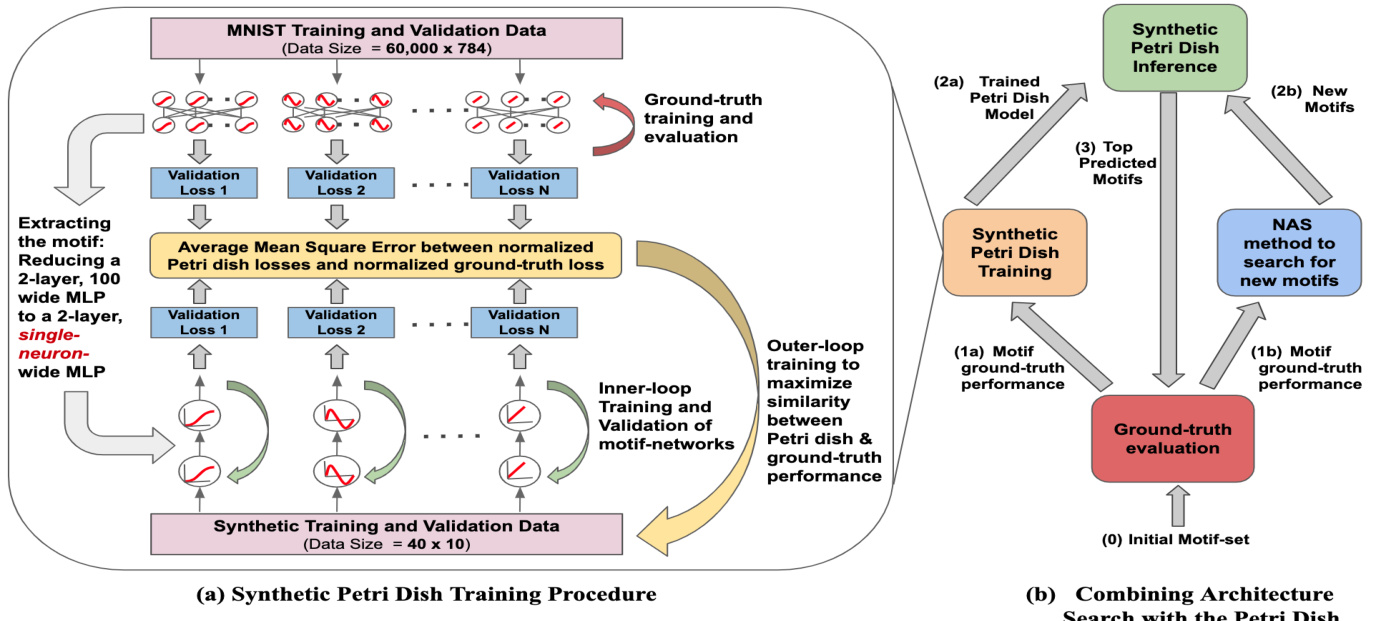
Figure 2. (a) Synthetic Petri Dish Training. The left figure illustrates the inner-loop and outer-loop training procedure. The motifs (in this example, activation functions) are extracted from the full network (e.g a 2-layer, 100 wide MLP) and instantiated in separate, much smaller motif-networks (e.g. a two-layer, single-neuron MLP). The motif-networks are trained in the inner-loop with the synthetic training data and evaluated using synthetic validation data. In the outer-loop, an average mean squared error loss is computed between the normalized Petri dish validation losses and the corresponding normalized ground-truth losses. Synthetic training and validation data are optimized by taking gradient steps w.r.t the outer-loop loss. (b) Combining Architecture Search with the Petri Dish. Functions are depicted inside rectangles and function outputs are depicted as arrows with their descriptions adjacent to them. At step b.0, an initial motif-set is trained and evaluated. The ground-truth performance for this initial set is used for Petri dish model training (step b.1a) and also to generate a set of new motifs through an NAS method like a GA or NAO (step b.1b). The trained Petri dish (step b.2a) model predicts the relative performance of the newly generated motifs (step b.2b) by running Petri dish model inference. A small subset of motifs, with the best predicted performance, are selected for ground-truth evaluation (a repetition of step b.0). These steps are repeated for several iterations and the architecture with the best ground-truth performance is obtained.
图 2: (a) 合成培养皿训练。左图展示了内循环与外循环的训练流程。从完整网络(例如一个2层100宽度的MLP)中提取出 motif(本例中为激活函数),并在独立的极小规模motif网络(例如一个2层单神经元的MLP)中实例化。这些motif网络在内循环中使用合成训练数据进行训练,并通过合成验证数据评估性能。在外循环中,计算归一化培养皿验证损失与对应归一化真实损失之间的平均均方误差。通过对外循环损失进行梯度下降来优化合成训练和验证数据。(b) 架构搜索与培养皿的结合。矩形框内表示函数,箭头表示函数输出并附带描述。步骤b.0中,对初始motif集进行训练和评估。该初始集的真实性能既用于培养皿模型训练(步骤b.1a),也通过遗传算法(GA)或NAO等NAS方法生成新motif集(步骤b.1b)。训练好的培养皿模型(步骤b.2a)通过推理预测新生成motif的相对性能(步骤b.2b)。筛选预测性能最优的少量motif进行真实评估(重复步骤b.0)。经过多次迭代后,可获得具有最佳真实性能的架构。
3.1. Training the Synthetic Petri Dish
3.1. 训练合成培养皿
To train the Synthetic Petri Dish first requires extracting the $N$ motifs from their ground-truth setting and instantiating each of them in miniature as separate motif-networks. For the experiments performed in this paper, the groundtruth network and the motif-network have the same overall blueprint and differ only in the width of their layers. For example, Figure 2a shows a ground-truth network’s size reduced from a 2-layer, 100-neuron wide MLP to a motifnetwork that is a 2-layer MLP with a single neuron per layer.
训练合成培养皿(Synthetic Petri Dish)首先需要从原始网络中提取N个模块(motif),并将每个模块实例化为独立的微型模块网络。本文实验中,原始网络与模块网络采用相同的整体架构,仅在各层宽度上存在差异。例如,图2a展示了将原始网络从2层100神经元宽度的多层感知机(MLP)缩减为每层仅含单个神经元的2层MLP模块网络。
Given such a collection of extracted motif-networks, a small number of synthetic training and validation data samples are then learned that can respectively be used to train and evaluate the motif-networks. The learning objective is that the validation loss of motifs trained in the Petri dish resemble the validation loss of the motif’s ground-truth evaluation $(\mathcal{L}_{t r u e}^{i})$ . Note that this training process requires two nested optimization loops: an inner-loop that trains and evaluates the motif-networks on the synthetic data and an outer-loop that trains the synthetic data itself.
给定这样一组提取出的基序网络(motif-network),随后学习少量合成的训练和验证数据样本,这些样本可分别用于训练和评估基序网络。学习目标是培养皿中训练的基序验证损失与其真实评估验证损失 $(\mathcal{L}_{t r u e}^{i})$ 相接近。需注意该训练过程需要两个嵌套优化循环:内循环负责在合成数据上训练和评估基序网络,外循环则负责优化合成数据本身。
Initializing the Synthetic Petri Dish: Before training the Petri dish, the motif-networks and synthetic data must be initialized. Once the motifs have been extracted into separate motif-networks, each motif-network is assigned the same initial random weights $(\theta_{i n i t})$ . This constraint reduces confounding factors by ensuring that the motif-networks differ from each other only in their instantiated motifs. At the start of Synthetic Petri Dish training, synthetic training data (Strain $(S^{t r a i n}=(x^{t r a i n},y^{t r a i n}))$ and validation data samples $(S^{v a l i d}=(x^{v a l i d},y^{v a l i d}))$ are randomly initialized. Note that these learned training and validation data can play distinct and complementary roles, e.g. the validation data can learn to test out-of-distribution generalization from a learned training set. Empirically, setting the training and validation data to be the same initially (i.e. $S^{t r a i n}=S^{v a l i d},$ benefited optimization at the beginning of outer-loop training; over iterations of outer-loop training, the synthetic training and validation data then diverge. The size of the motif-network and the number of synthetic data samples are chosen through the hyper parameter selection procedure
初始化合成培养皿:在训练培养皿之前,必须初始化基序网络(motif-networks)和合成数据。将基序提取到独立的基序网络后,每个基序网络被赋予相同的随机初始权重$(\theta_{i n i t})$。该约束通过确保基序网络仅在实例化基序上存在差异,从而减少混杂因素。合成培养皿训练开始时,随机初始化合成训练数据$(S^{t r a i n}=(x^{t r a i n},y^{t r a i n}))$和验证数据样本$(S^{v a l i d}=(x^{v a l i d},y^{v a l i d}))$。需注意,这些学习得到的训练和验证数据可发挥不同且互补的作用,例如验证数据可学习测试来自已学习训练集的分布外泛化能力。实证表明,初始时将训练和验证数据设为相同$(S^{t r a i n}=S^{v a l i d},)$有利于外循环训练初期的优化;随着外循环训练迭代,合成训练和验证数据会逐渐分化。基序网络的规模和合成数据样本数量通过超参数选择流程确定。
described in Appendix A.1.
附录A.1中所述。
Inner-loop training: The inner optimization loop is where the performance of motif-networks is evaluated by training each such network independently with synthetic data. This training reveals a sense of the quality of the motifs themselves.
内循环训练:内部优化循环通过使用合成数据独立训练每个基序网络(motif-network)来评估其性能,该训练过程能揭示基序本身的质量特性。
In each inner-loop, the motif-networks are independently trained with SGD using the synthetic training data $(S^{t r a i n})$ The motif-networks take synthetic training inputs $(x^{t r a i n})$ and produce their respective output predictions $(\hat{y}^{t r a i n})$ . For each motif-network, a binary cross-entropy (BCE) loss is computed between the output predictions $(\hat{y}^{t r a i n})$ and the synthetic training labels $(\boldsymbol{y}^{t r a i n})$ . Because the Petri dish is an artificial setting, the choice of BCE as the inner-loop loss $(\mathcal{L}_{i n n e r})$ is independent of the actual domain loss (used for ground-truth training), and other losses like regression loss could instead be used. The gradients of the BCE loss w.r.t. the motif-network weights inform weight updates (as in regular SGD).
在每个内部循环中,motif-network(模体网络)会使用合成训练数据$(S^{train})$通过SGD(随机梯度下降)进行独立训练。这些模体网络接收合成训练输入$(x^{train})$并生成各自的输出预测$(\hat{y}^{train})$。针对每个模体网络,会在输出预测$(\hat{y}^{train})$与合成训练标签$(\boldsymbol{y}^{train})$之间计算二元交叉熵(BCE)损失。由于培养皿是人工设定环境,选择BCE作为内部循环损失$(\mathcal{L}_{inner})$与实际领域损失(用于真实训练)无关,也可以使用回归损失等其他损失函数。BCE损失相对于模体网络权重的梯度决定了权重更新(与常规SGD相同)。
$$
\begin{array}{r}{\theta_{t+1}^{i}=\theta_{t}^{i}-\alpha\nabla\mathcal{L}_ {i n n e r_t r a i n}^{i}(S^{t r a i n},\theta_{t}^{i})\quad i\in{1,2,..,N}}\end{array}
$$
$$
\begin{array}{r}{\theta_{t+1}^{i}=\theta_{t}^{i}-\alpha\nabla\mathcal{L}_ {i n n e r_t r a i n}^{i}(S^{t r a i n},\theta_{t}^{i})\quad i\in{1,2,..,N}}\end{array}
$$
where $\alpha$ is the inner-loop learning rate and $\theta_{0}^{i}=~\theta_{i n i t}$ Inner-loop training proceeds until individual BCE losses converge. Once trained, each motif-network is independently evaluated using the synthetic validation data $(S^{v a l i d})$ to obtain individual validation loss values $(\mathcal{L}_{i n n e r_v a l i d}^{i})$ These inner-loop validation losses then enable calculating an outer-loop loss to optimize the synthetic data, which is described next.
其中 $\alpha$ 是内循环学习率,且 $\theta_{0}^{i}=~\theta_{i n i t}$。内循环训练持续进行,直到各BCE损失收敛。训练完成后,每个基序网络(motif-network)会使用合成验证数据 $(S^{v a l i d})$ 独立评估,以获得各自的验证损失值 $(\mathcal{L}_{i n n e r_v a l i d}^{i})$。这些内循环验证损失随后用于计算外循环损失以优化合成数据,具体方法如下所述。
Outer-loop training: Recall that an initial sampling of candidate motifs evaluated in the ground-truth setting serve as a training signal for crafting the Petri dish’s synthetic data. That is, in the outer loop, synthetic training data is optimized to encourage motif-networks trained upon it to become accurate surrogates for the performance of full networks built with that motif evaluated in the ground-truth setting. The idea is that training motif-networks on the right (small) set of synthetic training data can potentially isolate the key properties of candidate motifs that makes them effective. Consider for example what kind of training and validation examples would help to discover convolution. If an identical pattern appears in different training examples in three different quadrants, but not the fourth, the validation data could include an example in the fourth quadrant. Then, any convolutional (or translation invariant) architecture would pass this simple test, whereas others would perform poorly. In this way, generating synthetic training data could potentially have uncovered convolution, the key original architectural motif behind deep learning.
外循环训练:回顾在真实设定下评估的候选模块初始采样结果,这些结果可作为构建培养皿合成数据的训练信号。也就是说,在外循环中,优化合成训练数据是为了促使基于该数据训练的模块网络,能准确替代在真实设定下用该模块构建的完整网络性能。其核心思想是:在恰当的(少量)合成训练数据上训练模块网络,有望分离出候选模块的关键有效特性。例如设想什么样的训练和验证样本有助于发现卷积操作——若相同模式出现在三个不同象限的训练样本中而第四个象限没有,验证数据则可包含第四个象限的样本。此时,任何具备卷积(或平移不变)特性的架构都能通过这个简单测试,而其他架构则表现不佳。通过这种方式,生成合成训练数据本有可能揭示卷积这一深度学习背后的关键原始架构模块。
To frame the outer-loop loss function, what is desired is for the validation loss of the motif-network to induce the same relative ordering as the validation loss of the groundtruth networks; such relative ordering is all that is needed to decide which new motif is likely to be best. One way to design such an outer-loop loss with this property is to penalize differences between normalized loss values in the Petri dish and ground-truth setting1. To this end, the motifnetwork (inner-loop) loss values and their respective groundtruth loss values are first independently normalized to have zero-mean and unit-variance. Then, for each motif, a mean squared error (MSE) loss is computed between the normalized inner-loop validation loss $(\hat{\mathcal{L}}_ {i n n e r_v a l i d}^{i})$ and the normalized ground-truth validation loss $(\hat{\mathcal{L}}_{t r u e}^{i})$ . The MSE loss is averaged over all the motifs and used to compute a gradient step to improve the synthetic training and validation data.
为了构建外层循环的损失函数,关键在于使基序网络(motif-network)的验证损失能够产生与真实网络(groundtruth networks)验证损失相同的相对排序关系——这种相对排序正是决定哪个新基序可能最优所需的全部依据。实现该特性的一种设计方法是对培养皿环境与真实环境下归一化损失值的差异进行惩罚。具体而言,首先将基序网络(内层循环)损失值及其对应的真实损失值分别进行零均值单位方差的独立归一化。随后针对每个基序,计算归一化内层验证损失$(\hat{\mathcal{L}}_ {inner_valid}^{i})$与归一化真实验证损失$(\hat{\mathcal{L}}_{true}^{i})$之间的均方误差(MSE)损失。最终对所有基序的MSE损失取平均,并据此计算梯度步长以优化合成训练和验证数据。
$$
\mathcal{L}_ {o u t e r}=\frac{1}{N}\sum_{i=1}^{N}(\hat{\mathcal{L}}_ {i n n e r_v a l i d}^{i}-\hat{\mathcal{L}}_{t r u e}^{i})^{2}
$$
$$
\mathcal{L}_ {o u t e r}=\frac{1}{N}\sum_{i=1}^{N}(\hat{\mathcal{L}}_ {i n n e r_v a l i d}^{i}-\hat{\mathcal{L}}_{t r u e}^{i})^{2}
$$
$$
S_{t+1}^{t r a i n}=S_{t}^{t r a i n}-\beta\nabla\mathcal{L}_{o u t e r}
$$
$$
S_{t+1}^{t r a i n}=S_{t}^{t r a i n}-\beta\nabla\mathcal{L}_{o u t e r}
$$
$$
S_{t+1}^{v a l i d}=S_{t}^{v a l i d}-\beta\nabla\mathcal{L}_{o u t e r}
$$
$$
S_{t+1}^{v a l i d}=S_{t}^{v a l i d}-\beta\nabla\mathcal{L}_{o u t e r}
$$
where $\beta$ is the outer-loop learning rate. For simplicity, only the synthetic training $(x^{t r a i n})$ and validation $(x^{v a l i d})$ inputs are learned and the corresponding labels $(y^{t r a i n},y^{v a l i d})$ are kept fixed to their initial random values throughout training. Minimizing the outer-loop MSE loss $(\mathcal{L}_{o u t e r})$ modifies the synthetic training and validation inputs to maximize the similarity between the motif-networks’ performance ordering and motifs’ ground-truth ordering.
其中 $\beta$ 是外层循环的学习率。为简化流程,仅学习合成的训练输入 $(x^{train})$ 和验证输入 $(x^{valid})$,而对应的标签 $(y^{train},y^{valid})$ 在整个训练过程中保持初始随机值不变。通过最小化外层循环的均方误差损失 $(\mathcal{L}_{outer})$ 来调整合成的训练和验证输入,从而使基序网络(motif-network)的性能排序与基序真实排序之间的相似性最大化。
After each outer-loop training step, the motif-networks are reset to their original initial weights $(\theta_{i n i t})$ and the innerloop training and evaluation procedure (equation 1) is carried out again. The outer-loop of Synthetic Petri Dish training proceeds until the MSE loss converges, resulting in optimized synthetic data.
在每次外循环训练步骤后,基序网络(motif-networks)会重置为初始权重$(\theta_{init})$,并重新执行内循环训练与评估流程(公式1)。合成培养皿(Synthetic Petri Dish)训练的外循环会持续进行,直至均方误差(MSE)损失收敛,最终生成优化后的合成数据。
3.2. Predicting Performance with the Trained Petri Dish
3.2. 使用训练好的培养皿预测性能
The Synthetic Petri Dish training procedure described so far results in synthetic training and validation data optimized to sort motif-networks similarly to the ground-truth setting. This section describes how the trained Petri dish can predict the relative performance of unseen motifs, which we call the Synthetic Petri Dish inference procedure. In this procedure, new motifs are instantiated in their individual motif-networks, and the motif-networks are trained and evaluated using the optimized synthetic data (with the same hyper parameter settings as in the inner-loop training and evaluation). The relative inner-loop validation loss for the motif-networks then serves as a surrogate for the motifs’ relative ground-truth validation loss; as stated earlier, such relative loss values are sufficient to compare the potential of new candidate motifs. Such Petri dish inference is comput ation ally inexpensive because it involves the training and evaluation of very small motif-networks with very few synthetic examples. Accurately predicting the performance ordering of unseen motifs is contingent on the generalization capabilities of the Synthetic Petri Dish. The ability to generalize in this way is investigated in section 4.1.
目前所述的合成培养皿 (Synthetic Petri Dish) 训练流程能生成经过优化的合成训练与验证数据,使其对基序网络 (motif-network) 的排序结果与真实设定一致。本节将阐述训练后的培养皿如何预测未见基序的相对性能,我们称之为合成培养皿推理流程。该流程会为每个新基序实例化其独立的基序网络,并使用优化后的合成数据(保持与内循环训练和评估相同的超参数设置)对这些网络进行训练和评估。此时,基序网络的内循环验证损失相对值即可作为基序真实验证损失相对值的替代指标;如前所述,此类相对损失值足以用于比较新候选基序的潜力。这种培养皿推理的计算成本极低,因为它仅需用极少量合成样本训练和评估微型基序网络。准确预测未见基序的性能排序取决于合成培养皿的泛化能力,第4.1节将对此类泛化能力进行研究。
3.3. Combining Architecture Search with the Synthetic Petri Dish
3.3. 架构搜索与合成培养皿的结合
Interestingly, the cheap-to-evaluate surrogate performance prediction given by the trained Petri dish is complementary to most NAS methods that search for motifs, meaning that they can easily be combined. Algorithm 1 shows one possible hybridization of Petri dish and NAS, which is the one we experimentally investigate in this work.
有趣的是,由训练好的培养皿 (Petri dish) 提供的低成本替代性能预测与大多数搜索基序 (motif) 的神经架构搜索 (NAS) 方法具有互补性,这意味着它们可以轻松结合。算法1展示了一种可能的培养皿与NAS混合方案,这也是我们在本工作中实验验证的方法。
First, the Petri dish model is warm-started by training (innerloop and outer-loop) using the ground-truth evaluation data $(P_{e v a l})$ of a small set of randomly-generated motifs $(X_{e v a l})$ Then in each iteration of NAS, the NAS method generates $M$ new motifs and the Petri dish inference procedure inexpensively predicts their relative performance. The top $K$ motifs (where $K<<M,$ ) with highest predicted performance are then selected for ground-truth evaluation. The ground-truth performance of motifs both guides the NAS method as well as provides further data to re-train the Petri dish model. The steps outlined above are repeated for as many iterations as possible or until convergence and then the motif with the best ground-truth performance is selected for the final test evaluation.
首先,使用随机生成的一小组基序$(X_{eval})$的真实评估数据$(P_{eval})$对培养皿模型进行热身训练(内循环和外循环)。然后在神经架构搜索(NAS)的每次迭代中,NAS方法生成$M$个新基序,培养皿推理过程以低成本预测它们的相对性能。接着选择预测性能最高的前$K$个基序(其中$K<<M$)进行真实评估。这些基序的真实性能既指导NAS方法,又为重新训练培养皿模型提供更多数据。上述步骤会重复尽可能多的迭代次数或直到收敛,最终选择具有最佳真实性能的基序进行最终测试评估。
Synthetic Petri Dish training and inference is orders of magnitude faster than ground-truth evaluations, thus making NAS computationally more efficient and faster to run, which can enable finding higher-performing architectures given a limited compute budget. Further analysis of the compute overhead of the Petri dish model is in section 4.2.
合成培养皿 (Petri Dish) 的训练和推理速度比真实评估快几个数量级,从而使神经架构搜索 (NAS) 的计算效率更高、运行速度更快,在有限的计算预算下能够找到性能更优的架构。关于培养皿模型计算开销的进一步分析见第4.2节。
4. Experiments
4. 实验
The first experiment is the easily interpret able proof-ofconcept of searching for the optimal slope for the sigmoid, and the second is the challenging NAS problem of finding a high-performing recurrent cell for a language modeling task. The compute used to run these experiments included 20 Nvidia 1080Ti GPUs (for ground-truth training and evalua
第一次实验是可轻松解释的概念验证,旨在寻找S型函数的最优斜率;第二次实验则是具有挑战性的神经架构搜索(NAS)问题,需要为语言建模任务找到高性能的循环单元。实验运行使用了20块Nvidia 1080Ti GPU(用于基准训练和评估)。
Algorithm 1 Combining Architecture Search with the Synthetic Petri Dish
算法 1: 合成培养皿与架构搜索的结合
Output: The motif within $X$ with the best ground-truth performance.
输出:$X$ 中具有最佳真实性能的主题。
tion) and a MacBook CPU (for Synthetic Petri Dish training and inference).
在一台配备NVIDIA RTX 3090 GPU的Linux服务器(用于合成数据生成)和一台MacBook CPU(用于合成培养皿训练与推理)上运行。
4.1. Searching for the Optimal Slope for Sigmoidal Activation Functions
4.1. 寻找S型激活函数的最佳斜率
Preliminary experiments demonstrated that when a 2-layer, 100-wide feed-forward network with sigmoidal activation functions is trained on MNIST data, its validation accuracy (holding all else constant) depends on the slope of the sigmoid The points on the blue curve in Figure 1 demonstrate this fact, where the empirical peak performance is a slope of 0.23. This empirical dependence of performance on sigmoid slope provides an easy-to-understand context (where the optimal answer is known apriori) to clearly illustrate the advantage of the Synthetic Petri Dish. In more detail, we now explain an experiment in which sigmoid slope is the architectural motif to be explored in the Petri dish.
初步实验表明,当使用具有S型激活函数(sigmoidal activation functions)的2层100宽度前馈网络在MNIST数据上进行训练时,其验证准确率(保持其他条件不变)取决于S型函数的斜率。图1中的蓝色曲线点展示了这一现象,其中经验峰值性能对应的斜率为0.23。这种性能对S型斜率的经验依赖性为理解合成培养皿(Synthetic Petri Dish)的优势提供了直观场景(已知最优解的先验条件)。接下来我们将详细说明一个以S型斜率为探索目标的培养皿架构实验。
A subset of 30 ground-truth points (blue points in Figure 1, such that each ground-truth point is a tuple of sigmoid slope and the validation accuracy of the corresponding groundtruth MNIST network) are randomly selected from a restricted interval of sigmoid slope values (the blue-shaded region in Figure 1). These 30 ground-truth points are split into two equal parts to create training (15) and validation (15) datasets for both the Synthetic Petri Dish and the NNbased prediction model. The remaining ground-truth points (outside the blue-shaded region) are used only for testing.
从S型函数斜率值的限定区间内(图1中蓝色阴影区域)随机选取30个基准点(图1中的蓝色点,每个基准点均为S型函数斜率与对应基准MNIST网络验证准确率的元组),并将其均分为两部分,分别作为合成培养皿和基于神经网络的预测模型的训练集(15个)与验证集(15个)。其余基准点(蓝色阴影区域外)仅用于测试。
We compare Synthetic Petri Dish to the control of training a neural network surrogate model to predict performance as a function of sigmoid slope. This NN-based surrogate control is a 2-layer, 10-neuron-wide feed forward network that takes the sigmoid value as input and predicts the corresponding MNIST network validation accuracy as its output. A mean-squared error loss is computed between the predicted accuracy and the ground-truth validation accuracy, and the network is trained with the Adam optimizer. Hyperparameters for the NN-based model such as the network’s size, training batch-size (15), epochs of training (50), learning rate (0.001) and scale of initial random weights (0.1) were selected using the validation points. The predictions from the NN-model are normalized and plotted as the red-curve in Figure 1. Results demonstrate that the NN-based model overfits the training points, and poorly generalizes to the test points, completely failing to model the falloff to the left of the peak past the left of the blue-shaded region. As such, it predicts that performance is highest with a sigmoid slop near zero, whereas in fact performance at that point is extremely poor.
我们将 Synthetic Petri Dish 与训练神经网络代理模型来预测性能(作为 sigmoid 斜率的函数)的对照组进行比较。这种基于神经网络的对照组是一个 2 层、10 个神经元宽度的前馈网络,它以 sigmoid 值为输入,并预测相应的 MNIST 网络验证准确率作为输出。在预测准确率和真实验证准确率之间计算均方误差损失,并使用 Adam 优化器训练网络。基于神经网络的模型的超参数(如网络大小、训练批量大小 (15)、训练轮数 (50)、学习率 (0.001) 和初始随机权重规模 (0.1))均通过验证点选择。NN 模型的预测结果经过归一化后,在图 1 中以红色曲线绘制。结果表明,基于神经网络的模型对训练点过拟合,对测试点的泛化能力较差,完全无法模拟蓝色阴影区域左侧峰值后的下降趋势。因此,它预测 sigmoid 斜率接近零时性能最高,而实际上该点的性能极差。
For training the Synthetic Petri Dish model, each training motif (i.e. sigmoid with a unique slope value) is extracted from the MNIST network and instantiated in a 2-layer, single-neuron-wide motif-network $(\theta_{i n i t})$ . Thus, there are 15 motif-networks, one for each training point (the setup is similar to the one shown in Figure 2a). The input and output layers of the motif-network have a width of 10 each. A batch of synthetic training data (size $20\times10$ ) and a batch of synthetic validation data (size $20\times10^{\cdot}$ are initialized to the same initial random value (i.e. $S_{t r a i n}=S_{v a l i d},$ ). The motif-networks are trained in the inner-loop for $200\mathrm{SGD}$ steps and subsequently their performance on the synthetic validation data $(\mathcal{L}_{i n n e r_v a l i d}^{i})$ is used to compute outer-loop MSE loss w.r.t the ground-truth performance (as described in section 3.1). A total of 20 outer-loop training steps are performed. The model hyper parameters such as number of inner and outer-loop steps, size of the motif-network, size of synthetic data, inner and outer-loop learning rates (0.01 and 0.5 respectively), initial scale of motif-network random weights (1.0) are selected so that the MSE loss for 15 validation points is minimized (hyper parameter selection and other details for the two models are further described in Appendix A.2).
在训练合成培养皿(Synthetic Petri Dish)模型时,每个训练基元(即具有唯一斜率值的sigmoid函数)都从MNIST网络中提取,并在双层单神经元宽度的基元网络$(\theta_{init})$中实例化。因此共有15个基元网络,每个训练点对应一个(设置如图2a所示)。基元网络的输入层和输出层宽度均为10。合成训练数据批次(尺寸$20\times10$)和合成验证数据批次(尺寸$20\times10$)被初始化为相同的随机值(即$S_{train}=S_{valid}$)。基元网络在内循环中训练200步SGD,随后使用其在合成验证数据上的表现$(\mathcal{L}_{inner_valid}^{i})$来计算外循环MSE损失(如第3.1节所述)。共进行20步外循环训练。选择模型超参数(如内外循环步数、基元网络尺寸、合成数据尺寸、内外循环学习率(分别为0.01和0.5)、基元网络随机权重初始比例(1.0))以使15个验证点的MSE损失最小化(两个模型的超参数选择和其他细节详见附录A.2)。
During validation (and also during testing) of Petri dish, new motifs are instantiated in their own motif-networks and trained for 200 inner-loop steps. Thus, unlike the NN-based model that predicts the performance of new motifs based on their scalar value, the Synthetic Petri Dish trains and evaluates each new motif independently with synthetic data (i.e.
在培养皿验证(及测试)阶段,新基序会在专属基序网络中实例化,并通过200步内循环训练。因此,与基于神经网络(NN)通过标量值预测新基序性能的模型不同,合成培养皿会使用合成数据独立训练和评估每个新基序(即
it actually uses a NN with this particular sigmoidal slope in a small experiment and thus should have better information regarding how well this slope performs). The normalized predictions from the Synthetic Petri Dish are plotted as the green curve in Figure 1. The results show that Synthetic Petri Dish predictions accurately infer that there is a peak (including the falloff to its left) and also its approximate location. The NN surrogate model that is not exposed to the region with the peak could not be expected to infer the peak’s existence because its training data provides no basis for such a prediction, but the Synthetic Petri Dish is able to predict it because the motif itself is part of the Synthetic Petri Dish model, giving it a fundamental advantage, which is starkly illustrated in Figure 1.
它实际上在一个小实验中使用了一个具有特定S型斜率的神经网络 (NN),因此应该能更好地了解该斜率的表现如何。合成培养皿 (Synthetic Petri Dish) 的归一化预测结果在图1中以绿色曲线显示。结果表明,合成培养皿的预测准确推断出了峰值的存在(包括左侧的下降)及其大致位置。未接触峰值区域的NN替代模型无法推断出峰值的存在,因为其训练数据没有提供此类预测的基础,但合成培养皿能够预测到这一点,因为该主题本身就是合成培养皿模型的一部分,这赋予了它根本性的优势,这一点在图1中得到了鲜明体现。
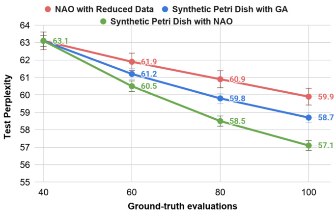
Figure 3. RNN Cell Search for PTB: This graph plots the test perplexity (mean of five runs) of the best found cell for three NAS methods across variable numbers of NAS iterations. All three methods are warmed up at the beginning (Step 0 in Figure 2b) with 40 ground-truth evaluations – notice the top-left point with best test perplexity of 63.1. For Synthetic Petri Dish with GA (blue curve) and Synthetic Petri Dish with NAO (green curve), the top 20 motifs with the best predicted performance are selected for ground-truth evaluations in each NAS iteration. Original NAO (Luo et al., 2018) (not shown here) requires 1,000 groundtruth evaluations to achieve a test perplexity of 56.0. NAO with Reduced Data (red-curve) shows the results obtained by running original NAO, but with fewer ground-truth evaluations (the same number the Synthetic Petri Dish variants get). With such limited data, Synthetic Petri Dish with NAO outperforms other NAS methods and achieves a test perplexity of 57.1 after 100 groundtruth evaluations.
图 3: PTB任务的RNN单元搜索:本图展示了三种神经架构搜索(NAS)方法在不同迭代次数下找到的最佳单元的测试困惑度(五次运行均值)。所有方法在初始阶段(图2b中的步骤0)都经过40次真实评估预热——注意左上角最佳测试困惑度为63.1的数据点。对于采用遗传算法(GA)的合成培养皿(蓝色曲线)和采用NAO的合成培养皿(绿色曲线),每次NAS迭代会选取预测性能最佳的20个基元进行真实评估。原始NAO方法(Luo et al., 2018)(未展示)需要1,000次真实评估才能达到56.0的测试困惑度。采用减少数据的NAO(红色曲线)展示了原始NAO在相同评估次数(与合成培养皿变体相同)下的结果。在数据有限的情况下,采用NAO的合成培养皿优于其他NAS方法,经过100次真实评估后达到了57.1的测试困惑度。
4.2. Architecture Search for Recurrent Cells
4.2. 循环单元架构搜索
The previous experiment demonstrated that a Synthetic Petri Dish model trained with limited ground-truth data can successfully generalize to unseen out-of-distribution motifs. This next experiment tests whether the Synthetic Petri Dish can be applied to a more realistic and challenging setting, that of NAS for a NN language model that is applied to the Penn Tree Bank (PTB) dataset – a popular language modeling and NAS benchmark (Marcus et al., 1993). In this experiment, the architectural motif is the design of a recurrent cell. The recurrent cell search space and its ground-truth evaluation setup is the same as in NAO (Luo et al., 2018). This NAS problem is challenging because the search space is expansive and few solutions perform well (Pham et al., 2018). Each cell in the search space is composed of 12 layers (each with the same layer width) that are connected in a unique pattern. An input embedding layer and an output soft-max layer is added to the cell (each of layer width 850) to obtain a full network (27 Million parameters) for ground-truth evaluation. Each ground-truth evaluation requires training on the PTB data-set for 600 epochs and takes 10 GPU hours on an Nvidia 1080Ti.
先前实验证明,使用有限真实数据训练的合成培养皿(Synthetic Petri Dish)模型能成功泛化到未见过的分布外基元。本实验将进一步测试该模型能否应用于更现实且更具挑战性的场景:针对宾州树库(PTB)数据集(语言建模与神经架构搜索(NAS)的常用基准[20])的神经网络语言模型NAS任务。本实验中,架构基元为循环单元设计,其搜索空间与真实评估设置均与NAO[18]保持一致。该NAS问题具有挑战性,因其搜索空间庞大且优质解决方案稀少[19]。搜索空间中每个单元由12层(每层宽度相同)以独特连接模式构成,通过添加输入嵌入层(层宽850)和输出softmax层(层宽850)形成完整网络(2700万参数)进行真实评估。每次真实评估需在PTB数据集上训练600个周期,耗时10个GPU小时(Nvidia 1080Ti)。
NAO is one of the state-of-the-art NAS methods for this problem and is therefore used as a baseline in this experiment (called here original NAO). Given the cell structure as input, NAO trains an LSTM model to encode and decode the cell structure, and also to predict its performance. Once trained, gradient ascent steps can be taken in the cell embedding space to optimize for RNN cells with higher performance. Thus, NAO consists of a performance-prediction model along with an implicit architecture optimization mechanism. In the published results (Luo et al., 2018), NAO is warm-started by training it on ground-truth evaluation data from 600 random RNN cells. In successive NAS iterations, NAO generates 200 new architectures, all of which are then evaluated for their ground-truth performance. At the end of three NAS iterations in which 1,000 groundtruth evaluations are performed (requiring 300 GPU days), NAO discovers a cell with test perplexity of 56.0. These are good results, but the compute cost even to reproduce them is prohibitively large for many researchers. Because the Synthetic Petri Dish offers a potential low-compute option, in this experiment, different NAS methods are compared instead in a setting where only limited ground-truth evaluation data is available $\leq100$ samples), giving a sense of how far different methods can get with more reasonable compute resources. Note that NAO can also be combined with weight-sharing (Pham et al., 2018) to improve its efficiency; however, to isolate the effect of the methods themselves from added factors such as weight-sharing (which can also be added in future work to the Synthetic Petri Dish), only methods without weight-sharing are compared.
NAO是该领域最先进的NAS方法之一,因此在本实验中作为基线(称为原始NAO)。该方法以细胞结构为输入,训练LSTM模型进行结构编码解码及性能预测。训练完成后,通过在细胞嵌入空间执行梯度上升步骤来优化RNN细胞性能。因此,NAO包含性能预测模型和隐式架构优化机制。已发表成果(Luo et al., 2018)显示,NAO通过600个随机RNN细胞的真实评估数据进行预热训练。在后续NAS迭代中,NAO每次生成200个新架构并进行真实性能评估。经过三轮迭代(共1,000次真实评估,耗时300 GPU天),最终发现的细胞测试困惑度为56.0。虽然结果优异,但复现所需的计算成本对多数研究者而言过高。由于合成培养皿(Synthetic Petri Dish)提供了低计算量方案,本实验改为在有限真实评估数据(≤100样本)环境下比较不同NAS方法,以评估各方法在合理计算资源下的表现。需说明的是,NAO也可结合权重共享(Pham et al., 2018)提升效率;但为排除权重共享等附加因素影响(未来工作也可将其引入合成培养皿),本实验仅比较未采用权重共享的方法。
Each NAS iteration can be accelerated if the number of costly ground-truth evaluations is reduced by instead cheaply evaluating the majority of candidate motifs (i.e. new cells) in the Petri dish. For the purpose of training the Synthetic Petri Dish, each cell is extracted from its ground-truth setting (850 neurons per layer) and is instantiated in a motif-network with three neurons per layer (its internal cell connectivity, including its depth, remains unchanged). Thus, the ground-truth network that has 27 million parameters is reduced to a motif-network with only 140 parameters. To train motif-networks, synthetic training and validation data each of size $20\times10\times10$ (batch size $\times$ time steps $\times$ motif-network input size) is learned (thus replacing the 923k training and 73k validation words of PTB). The Petri dish training and inference procedure is very similar to the one described in Experiment 4.1, and it adds negligible compute cost (2 additional hours for training, and a few minutes for inference on a MacBook CPU).
如果通过廉价评估培养皿中的大多数候选基序(即新单元)来减少成本高昂的真实评估次数,每次NAS迭代都可以加速。为了训练合成培养皿,每个单元从其真实设置(每层850个神经元)中提取,并在每层仅含三个神经元的基序网络中实例化(其内部单元连接性,包括深度,保持不变)。因此,拥有2700万个参数的真实网络被缩减为仅含140个参数的基序网络。训练基序网络时,使用大小为$20\times10\times10$(批量大小$\times$时间步长$\times$基序网络输入尺寸)的合成训练和验证数据进行学习(从而替代PTB的92.3万训练词和7.3万验证词)。培养皿的训练和推理过程与实验4.1所述非常相似,且增加的算力成本可忽略不计(训练额外耗时2小时,MacBook CPU上推理仅需几分钟)。
Following the steps outlined in algorithm 1 and Figure 2b, the Petri dish surrogate can be combined with two existing NAS methods: (1) genetic algorithms (GAs) or (2) NAO itself, resulting in two new methods called Synthetic Petri Dish-GA and Synthetic Petri Dish-NAO.
按照算法1和图2b所示的步骤,培养皿替代方法可以与两种现有的神经架构搜索(NAS)方法结合:(1) 遗传算法(GA) 或 (2) NAO本身,从而产生两种新方法:合成培养皿-GA和合成培养皿-NAO。
GA-based NAS methods have recently been found successful in several problem domains (Real et al., 2019; Elsken et al., 2019). In Synthetic Petri Dish-GA, RNN cell connectivity is represented as a string of numbers and therefore can be easily modified with GA operators such as point-wise mutation (rate $=0.05$ ) and crossover (rate $=0.3$ ) to generate new cells/motifs. Unlike GAs, the NAO method performs gradient-based search for new motifs. The gradients are potentially noisy and can result in low-performing motifs. Therefore, in principle adding the Synthetic Petri Dish to NAO can help filter of such low-performing motifs (thereby avoiding wasteful ground-truth evaluations). The details of hyper parameter selection for Synthetic Petri Dish-GA and Synthetic Petri Dish-NAO are provided in Appendix A.3.
基于遗传算法 (GA) 的神经架构搜索 (NAS) 方法近年来在多个问题领域取得了成功 [20][21]。在合成培养皿-GA中,RNN细胞连接性被表示为数字字符串,因此可以通过点突变 (概率=0.05) 和交叉 (概率=0.3) 等遗传算子轻松修改以生成新细胞/基序。与遗传算法不同,NAO方法采用基于梯度的搜索来寻找新基序。这些梯度可能存在噪声,可能导致生成低效基序。因此,原则上将合成培养皿引入NAO有助于过滤此类低效基序 (从而避免耗时的真实评估)。合成培养皿-GA和合成培养皿-NAO的超参数选择细节详见附录A.3。
For the Synthetic Petri Dish variants, at the beginning of search, both the Petri dish surrogate and the NAS method (GA/NAO) used within the Petri dish variant are warmstarted with the ground-truth data of an initial motif set (size 40). In each NAS iteration, 100 newly generated motifs (variable $M$ in algorithm 1) are evaluated using the Petri dish inference procedure and only the top 20 predicted motifs (variable $K$ in algorithm 1) are evaluated for their ground-truth performance. The test perplexity of the best found motif at the end of each NAS iteration is plotted in Figure 3 – the blue curve depicts the result for Synthetic Petri Dish-GA and green depicts the result for Synthetic Petri Dish-NAO. For a fair comparison, original NAO is re-run in this limited ground-truth setting and the resulting performance is depicted by the red-curve in Figure 3. The results show that Synthetic Petri Dish-NAO outperforms both Synthetic Petri Dish-GA and NAO when keeping the amount of ground-truth data points the same, suggesting that the Synthetic Petri Dish and NAO complement each other well. The hybridization of Synthetic Petri Dish and NAO finds a cell that is competitive in its performance (test perplexity 57.1) with original NAO (56.0), using only $1/10^{t h}$ of original NAO’s compute (and exceeds the performance of original NAO when both are given equivalent compute). The structure of this discovered cell is shown in Appendix A.3.
对于合成培养皿(Synthetic Petri Dish)变体,在搜索开始时,培养皿代理和内部使用的神经架构搜索(NAS)方法(GA/NAO)都通过初始基序集(规模40)的真实数据进行预热。每次NAS迭代中,使用培养皿推理程序评估100个新生成的基序(算法1中的变量$M$),并仅对预测得分前20的基序(算法1中的变量$K$)进行真实性能评估。图3绘制了每次NAS迭代结束时最佳基序的测试困惑度——蓝色曲线表示合成培养皿-GA的结果,绿色曲线表示合成培养皿-NAO的结果。为公平比较,原始NAO在此有限真实数据设置下重新运行,其性能结果由图3中红色曲线表示。结果表明,在保持相同真实数据量的情况下,合成培养皿-NAO优于合成培养皿-GA和原始NAO,说明合成培养皿与NAO能形成良好互补。合成培养皿与NAO的混合方法发现的细胞性能(测试困惑度57.1)与原始NAO(56.0)相当,仅消耗原始NAO$1/10^{t h}$的计算量(当计算量相同时甚至超越原始NAO性能)。该发现细胞的结构详见附录A.3。
5. Discussion and Conclusions
5. 讨论与结论
In the general practice of science, often the question arises of what factor accounts for an observed phenomenon. In the real world, with all its intricacy and complexity, it can be difficult to test or even formulate a clear hypothesis on the relevant factor involved. For that reason, often a hypothesis is formulated and tested in a simplified environment where the relevant factor can be isolated from the confounding complexity of the world around it. Then, in that simplified setting it becomes possible to run rapid and exhaustive tests, as long as there is an expectation that their outcome might correlate to the real world. In this way, the Synthetic Petri Dish is a kind of microcosm of a facet of the scientific method, and its synthetic data is the treatment whose optimization tethers the dynamics within the simplified setting to their relevant counterparts in the real world.
在科学研究的普遍实践中,经常会出现这样的问题:是什么因素导致了观察到的现象。在现实世界中,由于其错综复杂的特性,很难测试甚至明确表述出相关因素的假设。因此,通常会在一个简化的环境中提出并测试假设,以便将相关因素从周围世界的混杂复杂性中分离出来。然后,在这种简化的环境中,只要预期其结果可能与现实世界相关,就可以进行快速而详尽的测试。这样一来,合成培养皿 (Synthetic Petri Dish) 就成为了科学方法某一方面的缩影,而其合成数据则是优化手段,将简化环境中的动态与现实世界中的对应部分联系起来。
By approaching architecture search in this way as a kind of question-answering problem on how certain motifs or factors impact final results, we gain the intriguing advantage that the prediction model is no longer a black box. Instead, it actually contains within it a critical piece of the larger world that it seeks to predict. This piece, a motif cut from the ground-truth network (and its corresponding learning dynamics), carries with it from the start a set of priors that no naive black box learned model could carry on its own. These priors pop out dramatically in the simple sigmoid slope experiment – the notion that there is an optimal slope for training and roughly where it lies emerges automatically from the fact that the sigmoid slope itself is part of the Synthetic Petri Dish prediction model. In the later NAS for recurrent cells, the benefit in a more complex domain also becomes apparent, where the advantage of the intrinsic prior enables the Synthetic Petri Dish to have better performance than a leading NAS method when holding the number of ground-truth evaluations constant, and achieves roughly the same performance with $1/10^{\mathrm{th}}$ the compute when allowing differing numbers of ground-truth evaluations.
通过将架构搜索视为关于某些主题或因素如何影响最终结果的问答问题,我们获得了一个有趣的优势:预测模型不再是一个黑箱。相反,它实际上包含了其所预测的更广阔世界中的一个关键部分。这一部分是从真实网络中切割出的主题(及其对应的学习动态),从一开始就携带了一组先验知识,这是任何单纯通过学习的黑箱模型都无法独自承载的。这些先验在简单的S型函数斜率实验中表现得尤为明显——训练存在最优斜率的概念及其大致位置,这一认识自动浮现,正是因为S型函数斜率本身是合成培养皿预测模型的一部分。在后来的循环单元神经架构搜索中,更复杂领域的优势也变得显而易见:在保持真实评估次数不变的情况下,内在先验的优势使合成培养皿的性能优于领先的神经架构搜索方法;而在允许不同数量的真实评估时,仅需约$1/10^{\mathrm{th}}$的计算量就能达到大致相同的性能。
These benefits ultimately concern both computation and accuracy. Because the Synthetic Petri Dish contains a tiny version of the full problem, candidate architectures can be tested rapidly. Yet we do not give up the value of the surrogate in exchange for such efficiency; on the contrary, because the tiny model contains a piece of the real network (and hence enables testing various hypothesis as to its capabilities), the predictions are built on highly relevant priors that lend more accuracy to their results than blank-slate black box models.
这些优势最终涉及计算和准确性两方面。由于合成培养皿(Synthetic Petri Dish)包含了完整问题的微型版本,候选架构可以快速测试。然而我们并未为了效率而牺牲代理模型的价值;相反,由于微型模型包含真实网络的一部分(因此能测试关于其能力的各种假设),其预测基于高度相关的先验知识,这使得结果比从零开始的黑箱模型更为准确。
It is also possible that other methods can be built in the future on the idea of extracting a component of a candidate architecture and testing it in another setting. The opportunity to tease out the underlying causal factors of performance is a novel research direction that may ultimately teach us new lessons on architecture by exposing the most important dimensions of variation through a principled empirical process that could capture the spirit and power of the scientific process itself.
未来也可能基于提取候选架构组件并在其他环境中测试的思路开发出其他方法。通过严谨的实证过程揭示性能背后的因果因素,这一新颖研究方向有望发现架构变异的最关键维度,最终为我们带来关于架构设计的新认知,其方法论本身也蕴含着科学探索的精神与力量。
References
参考文献
Langley, P. Crafting papers on machine learning. In Langley, P. (ed.), Proceedings of the 17th International Conference on Machine Learning (ICML 2000), pp. 1207–1216, Stanford, CA, 2000. Morgan Kaufmann.
Langley, P. 撰写机器学习论文。见 Langley, P. (编), 《第17届国际机器学习会议论文集》(ICML 2000), 第1207–1216页, 斯坦福, 加利福尼亚州, 2000年. Morgan Kaufmann出版社。
Liu, C., Zoph, B., Neumann, M., Shlens, J., Hua, W., Li, L.-J., Fei-Fei, L., Yuille, A., Huang, J., and Murphy, K. Progressive neural architecture search. In Proceedings of the European Conference on Computer Vision (ECCV), pp. 19–34, 2018a.
Liu, C., Zoph, B., Neumann, M., Shlens, J., Hua, W., Li, L.-J., Fei-Fei, L., Yuille, A., Huang, J., and Murphy, K. 渐进式神经架构搜索。见《欧洲计算机视觉会议论文集》(ECCV),第19-34页,2018a。
Suganuma, M., Shirakawa, S., and Nagao, T. A genetic programming approach to designing convolutional neural network architectures. In Proceedings of the Genetic and Evolutionary Computation Conference, GECCO ’17, pp. 497–504, New York, NY, USA, 2017. ACM. ISBN 978-1-4503-4920-8. doi: 10.1145/3071178. 3071229. URL http://doi.acm.org/10.1145/ 3071178.3071229.
Suganuma, M., Shirakawa, S., and Nagao, T. 一种设计卷积神经网络架构的遗传编程方法。发表于《遗传与进化计算会议论文集》,GECCO '17,第497-504页,美国纽约州纽约市,2017年。ACM出版社。ISBN 978-1-4503-4920-8。doi: 10.1145/3071178.3071229。URL http://doi.acm.org/10.1145/3071178.3071229。
Zoph, B. and Le, Q. V. Neural architecture search with reinforcement learning. 2017. URL https://arxiv. org/abs/1611.01578.
Zoph, B. 和 Le, Q. V. 基于强化学习的神经架构搜索。2017. URL https://arxiv.org/abs/1611.01578.
A. Appendix
A. 附录
A.1. Petri dish Hyper parameter Selection Procedure
A.1. 培养皿超参数选择流程
Recall that an initial sampling of candidate motifs evaluated in the ground-truth setting serve as training data for Petri dish (Step 0 in Figure 2b). In order to determine the ideal hyper parameters for Petri dish training, this initial motif ground-truth set (referred to as $\mathcal{L}_ {t r u e}^{i}$ in Section 3) is split into equal parts as training $(\mathcal{L}_ {t r u e_t r a i n}^{i})$ and validation Litrue valid) sets. Hyper parameter setting that results in the smallest outer-loop MSE loss $\mathcal{L}_ {o u t e r}^{i}$ in equation 2) on the validation set $(\mathcal{L}_ {t r u e_v a l i d}^{i})$ after training the Petri dish on the training set $(\mathcal{L}_{t r u e_t r a i n}^{i})$ , are selected for the full experiment. Specific hyper parameter values for each experiment are provided in the following sections.
请注意,在真实设定下评估的候选基序初始采样结果将作为培养皿(图2b中的步骤0)的训练数据。为了确定培养皿训练的理想超参数,该初始基序真实集(第3节中记为$\mathcal{L}_ {t r u e}^{i}$)被均分为训练集$(\mathcal{L}_ {t r u e_t r a i n}^{i})$和验证集$(\mathcal{L}_ {t r u e_v a l i d}^{i})$。选择在训练集$(\mathcal{L}_ {t r u e_t r a i n}^{i})$上训练培养皿后,能使验证集$(\mathcal{L}_ {t r u e_v a l i d}^{i})$上外循环MSE损失$\mathcal{L}_{o u t e r}^{i}$(公式2)最小的超参数设置用于完整实验。具体实验的超参数值将在后续章节给出。
A.2. Experimental Setup for Optimal Sigmoid Slope Search
A.2. 最优S型函数斜率搜索实验设置
This section provides further details on experiment 4.1. The sigmoid slope value is the motif in this experiment.
本节进一步详述实验4.1,S型函数斜率值为本实验的核心变量。
A.2.1. SETUP FOR GROUND-TRUTH TRAINING
A.2.1. 真实训练数据设置
Previous work has shown that the slope of the sigmoid activation is a critical factor in determining network performance (Rama chandra n et al., 2018). Similarly, in this paper, it was empirically found that the validation performance of a 2-layer 100-wide feed forward network on MNIST dataset is dependent on the sigmoid slope. This dependence is shown by the blue-points in Figure 1. To generate each of the blue points, the feed forward network was trained on 50K MNIST training samples and evaluated on 10K validation samples, with the sigmoid slope value ranging between $0.01-2.01$ All other hyper parameters were held constant during each run and their specific values are provided in Table 1. For each slope value, a mean performance from 20 such runs (along with standard error bars) is plotted in Figure 1.
先前的研究表明,Sigmoid激活函数的斜率是决定网络性能的关键因素 (Ramachandran et al., 2018)。类似地,本文通过实验发现,在MNIST数据集上,一个2层100宽度的前馈网络的验证性能依赖于Sigmoid斜率。这种依赖性如图1中的蓝点所示。为了生成每个蓝点,前馈网络在50K个MNIST训练样本上进行训练,并在10K个验证样本上进行评估,Sigmoid斜率值范围在$0.01-2.01$之间。每次运行时所有其他超参数保持不变,具体值如表1所示。对于每个斜率值,图1中绘制了20次运行的平均性能(以及标准误差条)。
Table 1. Hyper parameter setting for training a 2-layer, 100-wide feed forward network to obtain ground-truth performance in Experiment 4.1.
| Hyperparameter | SearchRange | FinalSetting |
| Optimizer | N/A | Adam |
| Inner-looplearningrate | 0.001-0.01 | 0.01 |
| L2 weight penalty | 1e-5-1e-3 | 1e-5 |
| NumberofEpochs | 40-60 | 50 |
| BatchSize | 20,40,50,100 | 50 |
表 1: 实验4.1中用于训练2层100宽度前馈网络以获取基准性能的超参数设置
| 超参数 | 搜索范围 | 最终设置 |
|---|---|---|
| Optimizer | N/A | Adam |
| Inner-loop学习率 | 0.001-0.01 | 0.01 |
| L2权重惩罚 | 1e-5-1e-3 | 1e-5 |
| 训练轮数 | 40-60 | 50 |
| 批大小 | 20,40,50,100 | 50 |
A.2.2. SETUP FOR PETRI DISH TRAINING AND VALIDATION
A.2.2. 培养皿训练与验证设置
The hyper parameter selection procedure follows the same template as described in Section A.1. A subset of 30 groundtruth points are randomly selected from a restricted interval of sigmoid slope values ranging between 0.37-1.50 (bluepoints in the blue-shaded region of Figure 1). These 30 ground-truth points are split into two equal parts to create training (15) and validation data-set (15) for Petri dish hyper parameter selection. Hyper parameter search range and the final selected values are listed in Table 2.
超参数选择流程遵循与附录A.1章节相同的模板。从S型曲线斜率值限定区间0.37-1.50范围内随机选取30个基准点(对应图1蓝色阴影区域的蓝点)。这30个基准点被均分为两部分,分别构成培养皿超参数选择的训练集(15个点)和验证集(15个点)。超参数搜索范围及最终选定值列于表2。
Table 2. Hyper parameter setting for Petri dish training and inference in Experiment 4.1. Because the number of synthetic training samples is small (20), they are used in a single batch for Petri dish inner-loop training. The number of synthetic training samples is the same as the number of synthetic validation samples.
| Hyperparameter | Search Range | Final Setting |
| Inner-loop Optimizer | N/A | Adam |
| Motif-network input size | 10 | 10 |
| Motif-network output size | 10 | 10 |
| Motif-network hidden size | 1,3,5 | 1 |
| Synthetic training samples | 10,20 | 10 |
| Inner-loop learning rate | 0.001 -0.01 | 0.01 |
| Inner-loop L2 penalty | 1e-5-1e-3 | 1e-5 |
| Inner-loop training steps | 200,250 | 250 |
| Outer-loop Optimizer | N/A | Adam |
| Outer-loop learning rate | 0.01 - 0.05 | 0.05 |
| Outer-loop learning rate decay | 0.4- 0.8 | 0.4 |
| Outer-loop L2 penalty | 1e-5-1e-3 | 1e-5 |
| Outer-loop training steps | 20,40,60 | 60 |
表 2: 实验4.1中培养皿训练与推理的超参数设置。由于合成训练样本数量较少(20个),它们被用于单批次培养皿内循环训练。合成训练样本数量与合成验证样本数量相同。
| 超参数 | 搜索范围 | 最终设置 |
|---|---|---|
| 内循环优化器 | N/A | Adam |
| 基序网络输入尺寸 | 10 | 10 |
| 基序网络输出尺寸 | 10 | 10 |
| 基序网络隐藏层尺寸 | 1,3,5 | 1 |
| 合成训练样本数量 | 10,20 | 10 |
| 内循环学习率 | 0.001 -0.01 | 0.01 |
| 内循环L2正则项 | 1e-5-1e-3 | 1e-5 |
| 内循环训练步数 | 200,250 | 250 |
| 外循环优化器 | N/A | Adam |
| 外循环学习率 | 0.01 - 0.05 | 0.05 |
| 外循环学习率衰减 | 0.4- 0.8 | 0.4 |
| 外循环L2正则项 | 1e-5-1e-3 | 1e-5 |
| 外循环训练步数 | 20,40,60 | 60 |
At the beginning of Petri dish training, both the motifnetworks weights and the synthetic training/validation data are initialized to random values (drawn from normal distribution). The relative performance of motif-networks after inner-loop training on such random synthetic data is shown in Figure 4. This plot highlights that motif-network training extracts useful prior information about the corresponding motifs.
在培养皿训练初期,基序网络权重和合成训练/验证数据均被初始化为随机值(从正态分布中抽取)。图4展示了在此类随机合成数据上进行内循环训练后基序网络的相对性能。该图表凸显出基序网络训练能提取关于对应基序的有效先验信息。
Implementation Details: As described in Section 3, during Petri dish training, the motif-networks are independently trained and evaluated. Such independent training and evaluation is usually achieved by distributing network training on GPUs. However, because the motif-networks are very small (with only 22 parameters in each) and they share the same synthetic data, their training can be parallel i zed by a simple trick. The individual motif-networks can be combined to create a single super-network. With appropriate masking connections that prevent any forward and backward propagation across motif-networks within a super-network, we can ensure that all the motif-networks are independently trained at the same time during the super-network training. This parallel iz ation trick allows us to carry out Petri dish training and inference on a basic MacBook CPU very quickly.
实现细节:
如第3节所述,在培养皿训练期间,各基序网络(motif-network)独立进行训练和评估。这种独立训练和评估通常通过将网络训练分配到GPU上来实现。但由于基序网络非常小(每个仅含22个参数)且共享相同的合成数据,我们可以通过一个简单技巧实现并行化:将单个基序网络组合成一个超级网络。通过适当的掩码连接(防止超级网络内基序网络之间的前向/反向传播),可以确保所有基序网络在超级网络训练期间同步保持独立训练。这种并行化技巧使我们能在基础款MacBook CPU上快速完成培养皿训练与推理。

Figure 4. Relative performance of motif-networks with random synthetic data. The green curve shows the performance of motif-networks after inner-loop training on random data. This plot is similar to Figure 1 except that there is no Petri dish outer-loop training in this case.
图 4: 使用随机合成数据的 motif-network 相对性能。绿色曲线展示了 motif-network 在随机数据上进行内部循环训练后的性能表现。该图表与图 1 类似,区别在于本实验未进行培养皿外部循环训练。
A.2.3. SETUP FOR NN-BASED MODEL TRAINING
A.2.3. 基于神经网络 (NN) 的模型训练设置
The training and validation data for the NN-based model is exactly the same as the one used for Petri dish i.e. a set of 30 ground-truth points, where each point is a tuple of sigmoid slope and the validation accuracy of the corresponding ground-truth MNIST network. Similarly to the Petri dish, the NN-based model is trained to predict the normalized ground-truth performance (see Outer-loop training in Section 3). However, unlike Petri dish that trains and evaluates the motif (i.e. sigmoid slope) in a synthetic setting, the NNbased model takes the real-valued slope directly as its input. A mean squared error is computed between the NN predicted output and the normalized ground-truth performance. Hyper parameter search range and their final selected values are listed in Table 3.
基于神经网络 (NN) 模型的训练和验证数据与培养皿 (Petri dish) 所用完全相同,即一组30个真实标注点,每个点都是S型函数斜率与对应真实标注MNIST网络验证准确率的元组。与培养皿类似,该神经网络模型被训练用于预测归一化的真实性能(参见第3节中的外循环训练)。然而,不同于在合成环境中训练和评估基元(即S型斜率)的培养皿,基于神经网络的模型直接以实值斜率作为输入。通过计算神经网络预测输出与归一化真实性能之间的均方误差来确定损失。超参数搜索范围及其最终选定值列于表3。
A.3. Experiment Setup for Recurrent Cell Architecture Search
A.3. 循环单元架构搜索的实验设置
This section provides further details on experiment 4.2. The recurrent cell design is the motif in this experiment.
本节将进一步详述实验4.2的内容,其核心在于循环单元 (recurrent cell) 的设计。
A.3.1. SETUP FOR GROUND-TRUTH EVALUATION
A.3.1. 真实评估设置
Since NAO (Luo et al., 2018) is used as a baseline method for our experiments, the ground-truth training and evaluation procedure outlined in that paper is also followed here. The final test evaluation of the best found cell (output of Algorithm 1) is also carried out using the setting described
由于NAO (Luo et al., 2018) 被用作我们实验的基线方法,因此本文也遵循该论文中概述的真实训练和评估流程。最佳单元(算法1的输出)的最终测试评估同样采用所述设置进行。
Table 3. Hyper parameter setting for training the NN-based performance prediction model in Experiment 4.1.
| Hyperparameter | SearchRange | Final Setting |
| Optimizer | N/A | Adam |
| Networkhiddensize | 5,10,15,20 | 10 |
| Initial Learning rate | 0.001 -0.01 | 0.01 |
| Learning rate decay | 0.8 -0.99 | 0.97 |
| Learning rate decay steps | 50 -120 | 100 |
| L2 weight penalty | 1e-5-1e-3 | 1e-4 |
| Number of training steps | 100,150,200 | 150 |
| BatchSize | 15 | 15 |
表 3: 实验4.1中基于神经网络(NN)的性能预测模型训练超参数设置
| 超参数 | 搜索范围 | 最终设置 |
|---|---|---|
| 优化器(Optimizer) | N/A | Adam |
| 网络隐藏层大小 | 5,10,15,20 | 10 |
| 初始学习率 | 0.001 -0.01 | 0.01 |
| 学习率衰减率 | 0.8 -0.99 | 0.97 |
| 学习率衰减步数 | 50 -120 | 100 |
| L2权重惩罚项 | 1e-5-1e-3 | 1e-4 |
| 训练步数 | 100,150,200 | 150 |
| 批处理大小(BatchSize) | 15 | 15 |
in the NAO paper.
在NAO论文中。
A.3.2. SETUP FOR PETRI DISH TRAINING AND VALIDATION
A.3.2. 培养皿训练与验证设置
The hyper parameter selection procedure follows the same template as described in Section A.1. A set of 40 randomly selected cells are evaluated for their ground-truth performance. These 40 ground-truth points are split into two equal parts to create training (20) and validation data-set (20) for Petri dish hyper parameter selection. Hyper para meter search range and their final selected values are listed in Table 4.
超参数选择流程遵循附录A.1节所述的相同模板。随机选取40个细胞评估其真实性能,将这40个真实数据点均分为两部分:20个作为培养皿超参数选择的训练集,20个作为验证集。超参数搜索范围及最终选定值见表4。
Table 4. Hyper parameter setting for Petri dish training and inference in Experiment 4.2.
| Hyperparameter | Search Range | Final Set- ting |
| Inner-loop Optimizer Motif-network input size | N/A | Adam |
| Motif-networkoutputsize | 10 10 | 10 10 |
| Motif-network hidden size | 1,3,5 | 3 |
| Synthetic training size | 10,20 | 20 |
| Inner-loop learning rate | 0.001 -0.01 | 0.01 |
| Inner-loop L2 penalty | 1e-5-1e-3 | 1e-5 |
| Inner-loop training steps | 50,100 | 50 |
| Outer-loop Optimizer | N/A | |
| Outer-loop learning rate | 0.01-2.5 | Adam |
| Outer-loop learning rate decay | 2.0 | |
| Outer-loop L2 penalty Outer-loop training steps | 0.4-0.8 1e-6-1e-3 100, 200,300 | 0.5 5e-5 |
表 4: 实验4.2中培养皿训练与推理的超参数设置
| 超参数 | 搜索范围 | 最终设置 |
|---|---|---|
| 内循环优化器 | N/A | Adam |
| 基序网络输入尺寸 | 10 10 | 10 10 |
| 基序网络输出尺寸 | 10 10 | 10 10 |
| 基序网络隐藏层大小 | 1,3,5 | 3 |
| 合成训练集大小 | 10,20 | 20 |
| 内循环学习率 | 0.001-0.01 | 0.01 |
| 内循环L2正则项 | 1e-5-1e-3 | 1e-5 |
| 内循环训练步数 | 50,100 | 50 |
| 外循环优化器 | N/A | Adam |
| 外循环学习率 | 0.01-2.5 | 2.0 |
| 外循环学习率衰减 | 0.4-0.8 | 0.5 |
| 外循环L2正则项 | 1e-6-1e-3 | 5e-5 |
| 外循环训练步数 | 100,200,300 | 200 |
Implementation Details: The parallel iz ation trick of combining multiple motif-networks into a single super-network as described in Appendix A.2.2, is also utilized here as well. Experiment 4.1 required only a single NAS iteration i.e. training Petri dish with a fixed number of training motifs (and their corresponding ground-truth values) and then predicting the performance of test motifs. Unlike Experiment 4.1, in Experiment 4.2, the number of training motifs increase with additional ground-truth evaluations in each NAS iteration. For example, at the end of three such NAS iterations, there are 100 training motifs that can be utilized for Petri dish training. A growing number of motifnetworks during Petri dish training could require further hyper parameter tuning. To avoid such fine-tuning, the total number of motif-network instances during Petri dish training is kept fixed at 40 (thereby also limiting the size of the super-network). During each outer-loop training step, a new batch of 40 motif-networks are randomly sampled from the full-set of available motif-networks.
实现细节:这里同样采用了附录A.2.2中描述的并行化技巧,即将多个基序网络组合成单个超级网络。实验4.1仅需单次神经架构搜索(NAS)迭代,即用固定数量的训练基序(及其对应真实值)训练培养皿(Petri dish),然后预测测试基序的性能。与实验4.1不同,实验4.2中训练基序数量会随着每次NAS迭代新增的真实值评估而增加。例如,在完成三次此类NAS迭代后,就有100个训练基序可用于培养皿训练。培养皿训练期间不断增长的基序网络数量可能需要进一步超参数调优。为避免此类微调,培养皿训练期间的基序网络实例总数固定为40个(从而也限制了超级网络的规模)。在每次外循环训练步骤中,会从全部可用基序网络中随机采样新一批40个基序网络。
A.3.3. SETUP FOR NAO AND GA
A.3.3. NAO和GA的设置
In Experiment 4.2, two variants of NAO are evaluated in limited resource setting – NAO with Reduced data (redcurve in Figure 3) and Synthetic Petri Dish-NAO (green curve in Figure 3). For both the variants, the NAO model is trained with the same code and hyper parameter setting as in the published work (Luo et al., 2018).
在实验4.2中,我们在有限资源设置下评估了NAO的两个变体——数据缩减版NAO (图3中的红色曲线)和合成培养皿版NAO (图3中的绿色曲线)。两个变体都采用与已发表工作(Luo et al., 2018)相同的代码和超参数设置进行训练。
An elitist genetic algorithm (GA) is used to generate new motifs for the Synthetic Petri Dish-GA method (blue curve in Figure 3). In each NAS iteration, the top 20 motifs (with the best ground-truth values) are mutated and recombined to generate 100 new motifs. Each motif is represented as a fixed-size string of numbers that encode the cell connectivity and the types of non-linearity within the cell. During the mutation of a motif, every location within its string is modified with a probability of 0.05. During recombination, two randomly selected motifs are crossed-over at a random location in their strings with a probability of 0.3.
采用精英遗传算法 (GA) 为 Synthetic Petri Dish-GA 方法生成新基元 (图 3 中蓝色曲线)。在每次 NAS (神经架构搜索) 迭代中,前 20 个基元 (具有最佳真实值) 会经过变异和重组生成 100 个新基元。每个基元表示为固定长度的数字串,编码了单元连接性和单元内非线性类型。基元变异时,其数字串中每个位置有 0.05 概率被修改;重组时,两个随机选择的基元有 0.3 概率在其数字串的随机位置进行交叉。
The best found cell using the Synthetic Petri Dish-NAO method has a test perplexity of 57.1 and is shown in Figure 5.
使用Synthetic Petri Dish-NAO方法找到的最佳单元测试困惑度为57.1,如图5所示。

Figure 5. Best Cell found by Synthetic Petri Dish-NAO method.
图 5: 合成培养皿-NAO方法发现的最佳细胞。