Movement Pruning: Adaptive Sparsity by Fine-Tuning
Movement Pruning: 通过微调实现自适应稀疏化
Victor Sanh1, Thomas Wolf1, Alexander M. Rush1,2 1Hugging Face, 2Cornell University {victor,thomas}@hugging face.co ; arush@cornell.edu
Victor Sanh1, Thomas Wolf1, Alexander M. Rush1,2 1Hugging Face, 2Cornell University {victor,thomas}@huggingface.co ; arush@cornell.edu
Abstract
摘要
Magnitude pruning is a widely used strategy for reducing model size in pure supervised learning; however, it is less effective in the transfer learning regime that has become standard for state-of-the-art natural language processing applications. We propose the use of movement pruning, a simple, deterministic first-order weight pruning method that is more adaptive to pretrained model fine-tuning. We give mathematical foundations to the method and compare it to existing zeroth- and first-order pruning methods. Experiments show that when pruning large pretrained language models, movement pruning shows significant improvements in highsparsity regimes. When combined with distillation, the approach achieves minimal accuracy loss with down to only $3%$ of the model parameters.
幅度剪枝 (magnitude pruning) 是一种广泛用于纯监督学习模型压缩的策略,但在已成为最先进自然语言处理应用标准的迁移学习场景中效果欠佳。我们提出运动剪枝 (movement pruning) 方法,这是一种简单、确定性的—阶权重剪枝方法,能更好地适应预训练模型微调场景。我们为该算法建立了数学基础,并与现有零阶和一阶剪枝方法进行了对比实验。结果表明,在对大型预训练语言模型进行剪枝时,运动剪枝在高稀疏度场景下表现出显著优势。当结合知识蒸馏技术时,该方法仅保留 $3%$ 模型参数即可实现精度损失最小化。
1 Introduction
1 引言
Large-scale transfer learning has become ubiquitous in deep learning and achieves state-of-the-art performance in applications in natural language processing and related fields. In this setup, a large model pretrained on a massive generic dataset is then fine-tuned on a smaller annotated dataset to perform a specific end-task. Model accuracy has been shown to scale with the pretrained model and dataset size [Raffel et al., 2019]. However, significant resources are required to ship and deploy these large models, and training the models have high environmental costs [Strubell et al., 2019].
大规模迁移学习在深度学习中已变得无处不在,并在自然语言处理及相关领域的应用中实现了最先进的性能。在这种设置下,先在庞大的通用数据集上预训练一个大模型,然后在较小的标注数据集上进行微调,以执行特定的终端任务。研究表明,模型准确率会随着预训练模型和数据集的规模提升而提高 [Raffel et al., 2019]。然而,部署这些大模型需要耗费大量资源,且训练过程会产生高昂的环境成本 [Strubell et al., 2019]。
Sparsity induction is a widely used approach to reduce the memory footprint of neural networks at only a small cost of accuracy. Pruning methods, which remove weights based on their importance, are a particularly simple and effective method for compressing models. Smaller models are easier to sent on edge devices such as mobile phones but are also significantly less energy greedy: the majority of the energy consumption comes from fetching the model parameters from the long term storage of the mobile device to its volatile memory [Han et al., 2016a, Horowitz, 2014].
稀疏化 (sparsity induction) 是一种广泛使用的技术,能以微小精度代价降低神经网络的内存占用。剪枝 (pruning) 方法通过移除低重要性权重来压缩模型,是一种简单高效的模型压缩手段。轻量化模型更易于部署至手机等边缘设备,同时能显著降低能耗:移动设备的主要能耗来源于将模型参数从长期存储载入易失性内存的过程 [Han et al., 2016a, Horowitz, 2014]。
Magnitude pruning [Han et al., 2015, 2016b], which preserves weights with high absolute values, is the most widely used method for weight pruning. It has been applied to a large variety of architectures in computer vision [Guo et al., 2016], in language processing [Gale et al., 2019], and more recently has been leveraged as a core component in the lottery ticket hypothesis [Frankle et al., 2020].
幅度剪枝 (magnitude pruning) [Han et al., 2015, 2016b] 通过保留绝对值较大的权重,成为权重剪枝中最广泛使用的方法。该方法已应用于计算机视觉 [Guo et al., 2016] 和语言处理 [Gale et al., 2019] 等多种架构,最近更被用作彩票假设 (lottery ticket hypothesis) [Frankle et al., 2020] 的核心组件。
While magnitude pruning is highly effective for standard supervised learning, it is inherently less useful in the transfer learning regime. In supervised learning, weight values are primarily determined by the end-task training data. In transfer learning, weight values are mostly predetermined by the original model and are only fine-tuned on the end task. This prevents these methods from learning to prune based on the fine-tuning step, or “fine-pruning.”
虽然幅度剪枝在标准监督学习中非常有效,但在迁移学习场景中本质上作用有限。监督学习的权重值主要由终端任务训练数据决定,而迁移学习的权重值大多由原始模型预先确定,仅针对终端任务进行微调。这导致此类方法无法基于微调步骤学习剪枝策略,即"微剪枝(fine-pruning)"。
In this work, we argue that to effectively reduce the size of models for transfer learning, one should instead use movement pruning, i.e., pruning approaches that consider the changes in weights during fine-tuning. Movement pruning differs from magnitude pruning in that both weights with low and high values can be pruned if they shrink during training. This strategy moves the selection criteria from the 0th to the 1st-order and facilitates greater pruning based on the fine-tuning objective. To test this approach, we introduce a particularly simple, deterministic version of movement pruning utilizing the straight-through estimator [Bengio et al., 2013].
在本工作中,我们提出要有效缩减迁移学习模型的规模,应采用动态剪枝(movement pruning)方法,即在微调过程中根据权重变化进行剪枝的策略。动态剪枝与幅度剪枝(magnitude pruning)的本质区别在于:只要权重在训练过程中缩小,无论其初始值高低都可能被剪除。该策略将选择标准从零阶提升至一阶,能基于微调目标实现更彻底的剪枝。为验证此方法,我们采用直通估计器[Bengio et al., 2013]实现了一种特别简单的确定性动态剪枝方案。
We apply movement pruning to pretrained language representations (BERT) [Devlin et al., 2019, Vaswani et al., 2017] on a diverse set of fine-tuning tasks. In highly sparse regimes (less than $15%$ of remaining weights), we observe significant improvements over magnitude pruning and other 1st-order methods such as $L_{0}$ regular iz ation [Louizos et al., 2017]. Our models reach $95%$ of the original BERT performance with only $5%$ of the encoder’s weight on natural language inference (MNLI) [Williams et al., 2018] and question answering (SQuAD v1.1) [Rajpurkar et al., 2016]. Analysis of the differences between magnitude pruning and movement pruning shows that the two methods lead to radically different pruned models with movement pruning showing greater ability to adapt to the end-task.
我们在多样化的微调任务上对预训练语言表示(BERT) [Devlin et al., 2019, Vaswani et al., 2017] 应用了动态剪枝。在高稀疏度场景(保留权重少于15%)下,我们观察到该方法显著优于幅度剪枝和其他一阶方法(如L0正则化 [Louizos et al., 2017])。在自然语言推理(MNLI) [Williams et al., 2018] 和问答任务(SQuAD v1.1) [Rajpurkar et al., 2016] 中,我们的模型仅保留编码器5%权重即可达到原始BERT性能的95%。对比分析表明,幅度剪枝与动态剪枝会产生截然不同的剪枝模型,其中动态剪枝展现出更强的任务适应能力。
2 Related Work
2 相关工作
In addition to magnitude pruning, there are many other approaches for generic model weight pruning. Most similar to our approach are methods for using parallel score matrices to augment the weight matrices [Mallya and Lazebnik, 2018, Ramanujan et al., 2020], which have been applied for convolutional networks. Differing from our methods, these methods keep the weights of the model fixed (either from a randomly initialized network or a pre-trained network) and the scores are updated to find a good sparse subnetwork.
除了幅度剪枝外,还有许多其他通用模型权重剪枝方法。与我们的方法最相似的是使用并行评分矩阵来增强权重矩阵的技术 [Mallya and Lazebnik, 2018, Ramanujan et al., 2020],这些方法已应用于卷积网络。与我们的方法不同,这些方法保持模型的权重固定(无论是随机初始化网络还是预训练网络),并通过更新评分来寻找良好的稀疏子网络。
Many previous works have also explored using higher-order information to select prunable weights. LeCun et al. [1989] and Hassibi et al. [1993] leverage the Hessian of the loss to select weights for deletion. Our method does not require the (possibly costly) computation of second-order derivatives since the importance scores are obtained simply as the by-product of the standard fine-tuning. [Theis et al., 2018, Ding et al., 2019, Lee et al., 2019] use the absolute value or the square value of the gradient. In contrast, we found it useful to preserve the direction of movement in our algorithm.
许多先前的研究也探索了利用高阶信息来选择可剪枝权重。LeCun等人[1989]和Hassibi等人[1993]利用损失函数的Hessian矩阵来选择待删除权重。我们的方法不需要(可能计算成本较高的)二阶导数计算,因为重要性分数仅作为标准微调的副产品即可获得。[Theis等人, 2018, Ding等人, 2019, Lee等人, 2019]使用梯度的绝对值或平方值。相比之下,我们发现保留算法中移动方向的做法更具实用性。
Compressing pretrained language models for transfer learning is also a popular area of study. Other approaches include knowledge distillation [Sanh et al., 2019, Tang et al., 2019] and structured pruning [Fan et al., 2020a, Sajjad et al., 2020, Michel et al., 2019, Wang et al., 2019]. Our core method does not require an external teacher model and targets individual weight. We also show that having a teacher can further improve our approach. Recent work also builds upon iterative magnitude pruning with rewinding [Yu et al., 2020], weight redistribution [Dettmers and Z ett le moyer, 2019] models from scratch. This differs from our approach which we frame in the context of transfer learning (focusing on the fine-tuning stage). Finally, another popular compression approach is quantization. Quantization has been applied to a variety of modern large architectures [Fan et al., 2020b, Zafrir et al., 2019, Gong et al., 2014] providing high memory compression rates at the cost of no or little performance. As shown in previous works [Li et al., 2020, Han et al., 2016b] quantization and pruning are complimentary and can be combined to further improve the performance/size ratio.
压缩预训练语言模型以进行迁移学习也是一个热门研究领域。其他方法包括知识蒸馏 [Sanh et al., 2019, Tang et al., 2019] 和结构化剪枝 [Fan et al., 2020a, Sajjad et al., 2020, Michel et al., 2019, Wang et al., 2019]。我们的核心方法不需要外部教师模型,且针对单个权重进行操作。我们还证明引入教师模型能进一步提升该方法。近期研究也基于带权重回退的迭代幅度剪枝 [Yu et al., 2020]、权重重分配 [Dettmers and Zettlemoyer, 2019] 从头训练模型。这与我们在迁移学习框架下(专注于微调阶段)的方法不同。最后,另一种主流压缩方法是量化。量化技术已应用于多种现代大型架构 [Fan et al., 2020b, Zafrir et al., 2019, Gong et al., 2014],能在几乎不损失性能的前提下实现高内存压缩率。如先前工作所示 [Li et al., 2020, Han et al., 2016b],量化与剪枝具有互补性,结合使用可进一步提升性能/体积比。
3 Background: Score-Based Pruning
3 背景:基于分数的剪枝
We first establish shared notation for discussing different neural network pruning strategies. Let $\mathbf{W}\in\mathbb{R}^{n\times n}$ refer to a generic weight matrix in the model (we consider square matrices, but they could be of any shape). To determine which weights are pruned, we introduce a parallel matrix of associated importance scores $\mathbf{S}\in\mathbb{R}^{n\times n}$ . Given importance scores, each pruning strategy computes a mask $\mathbf{M}\in{\bar{0},1}^{n\times n}$ . Inference for an input $\mathbf{x}$ becomes $\mathbf{a}=(\mathbf{W}\odot\mathbf{M})\mathbf{x}$ , where $\odot$ is the Hadamard product. A common strategy is to keep the top $v$ percent of weights by importance. We define $\mathrm{Top}_{v}$ as a function which selects the $v%$ highest values in S:
我们首先建立用于讨论不同神经网络剪枝策略的统一符号表示。设 $\mathbf{W}\in\mathbb{R}^{n\times n}$ 表示模型中的通用权重矩阵(我们考虑方阵,但也可以是任意形状)。为了确定剪枝哪些权重,我们引入一个对应的权重重要性分数矩阵 $\mathbf{S}\in\mathbb{R}^{n\times n}$。给定重要性分数后,每个剪枝策略会计算一个掩码 $\mathbf{M}\in{\bar{0},1}^{n\times n}$。对于输入 $\mathbf{x}$ 的推理过程变为 $\mathbf{a}=(\mathbf{W}\odot\mathbf{M})\mathbf{x}$,其中 $\odot$ 表示哈达玛积。常见策略是保留重要性前 $v$ 百分比的权重。我们定义 $\mathrm{Top}_{v}$ 为选择 S 中前 $v%$ 最高值的函数:
$$
\text{Top}_ v(\mathbf{S})_ {i,j} =
\begin{cases}
1, & S_{i,j} \text{ in top } v\% \\
0, & \text{o.w.}
\end{cases}
$$
$$
\text{Top}_ v(\mathbf{S})_ {i,j} =
\begin{cases}
1, & S_{i,j} \text{ in top } v\% \\
0, & \text{o.w.}
\end{cases}
$$
Magnitude-based weight pruning determines the mask based on the absolute value of each weight as a measure of importance. Formally, we have importance scores $\mathbf{S}=\left(|W_{i,j}|\right)_ {1\leq i,j\leq n}$ , and masks $\mathbf{M}=\mathrm{Top}_{v}(\mathbf{S})$ (Eq (1)). There are several extensions to this base setup. Han et al. [2015] use iterative magnitude pruning: the model is first trained until convergence and weights with the lowest magnitudes are removed afterward. The sparsified model is then re-trained with the removed weights fixed to 0. This loop is repeated until the desired sparsity level is reached.
基于幅度的权重剪枝根据每个权重的绝对值作为重要性度量来确定掩码。形式上,重要性分数为 $\mathbf{S}=\left(|W_{i,j}|\right)_ {1\leq i,j\leq n}$,掩码为 $\mathbf{M}=\mathrm{Top}_{v}(\mathbf{S})$(公式(1))。这一基础设置有几个扩展。Han等人[2015]采用迭代幅度剪枝:首先训练模型直至收敛,然后移除幅度最低的权重。接着,将剪枝后的模型重新训练,并将移除的权重固定为0。重复此循环直至达到目标稀疏度。
| Magnitudepruning | Lo regularization | Movementpruning | Softmovementpruning | |
| PruningDecision | Othorder | 1st order | 1storder | 1st order |
| Masking Function | Topu | ContinuousHard-Concrete | Topu | Thresholding |
| PruningStructure | LocalorGlobal | Global | LocalorGlobal | Global |
| Learning Objective | C | C+入oE(Lo) | C | C + 入mvpR(S) |
| GradientForm | Gumbel-Softmax | Straight-Through | Straight-Through | |
| ScoresS | Wi.j | -∑t( ac (M()( f(S(t) awi. | -Zt(aW. aC ()M(2)( | -∑t( aC (z)M() aWi. |
Table 1: Summary of the pruning methods considered in this work and their specific i ties. The expression of $f$ of $L_{0}$ regular iz ation is detailed in Eq (4).
| 幅度剪枝 (Magnitude pruning) | L0正则化 (Lo regularization) | 动态剪枝 (Movement pruning) | 软动态剪枝 (Soft movement pruning) | |
|---|---|---|---|---|
| 剪枝决策 (Pruning Decision) | 零阶 (0th order) | 一阶 (1st order) | 一阶 (1st order) | 一阶 (1st order) |
| 掩码函数 (Masking Function) | Top-k | 连续硬混凝土 (Continuous Hard-Concrete) | Top-k | 阈值法 (Thresholding) |
| 剪枝结构 (Pruning Structure) | 局部或全局 (Local or Global) | 全局 (Global) | 局部或全局 (Local or Global) | 全局 (Global) |
| 学习目标 (Learning Objective) | C | C + λE(L0) | C | C + λmvpR(S) |
| 梯度形式 (Gradient Form) | Gumbel-Softmax | 直通式 (Straight-Through) | 直通式 (Straight-Through) | |
| 分数S (Scores S) | Wi,j | -∑t(∂C/∂M(t))(f(S(t))/∂Wi,j) | -∑t(∂C/∂M(t))(∂M(t)/∂Wi,j) | -∑t(∂C/∂M(t))(∂M(t)/∂Wi,j) |
表 1: 本文考虑的剪枝方法及其特性的总结。L0正则化的表达式f在公式(4)中有详细说明。
In this study, we focus on automated gradual pruning [Zhu and Gupta, 2018]. It supplements magnitude pruning by allowing masked weights to be updated such that they are not fixed for the entire duration of the training. Automated gradual pruning enables the model to recover from previous masking choices [Guo et al., 2016]. In addition, one can gradually increases the sparsity level $v$ during training using a cubic sparsity scheduler: $\begin{array}{r}{v^{(t)}=\overset{^{-}}{v_{f}}+\left(v_{i}-\overset{^{}}{v}_ {f}\right)\left(1-\frac{t-t_{i}}{N\Delta t}\right)^{\bar{3}}}\end{array}$ . The sparsity level at time step $t$ , $v^{(t)}$ is increased from an initial value $v_{i}$ (usually 0) to a final value $v_{f}$ in $n$ pruning steps after $t_{i}$ steps of warm-up. The model is thus pruned and trained jointly.
在本研究中,我们专注于自动渐进剪枝(automated gradual pruning)[Zhu and Gupta, 2018]。该方法对幅度剪枝进行了补充,允许被掩码的权重在整个训练过程中持续更新而非固定不变。自动渐进剪枝使模型能够从先前的掩码选择中恢复[Guo et al., 2016]。此外,可通过立方稀疏度调度器在训练期间逐步提升稀疏度$v$:$\begin{array}{r}{v^{(t)}=\overset{^{-}}{v_{f}}+\left(v_{i}-\overset{^{}}{v}_ {f}\right)\left(1-\frac{t-t_{i}}{N\Delta t}\right)^{\bar{3}}}\end{array}$。时间步$t$对应的稀疏度$v^{(t)}$从初始值$v_{i}$(通常为0)经$n$次剪枝步骤逐步提升至最终值$v_{f}$,该过程始于预热阶段$t_{i}$步之后。模型因此实现了剪枝与训练的同步进行。
4 Movement Pruning
4 动态剪枝 (Movement Pruning)
Magnitude pruning can be seen as utilizing zeroth-order information (absolute value) of the running model. In this work, we focus on movement pruning methods where importance is derived from first-order information. Intuitively, instead of selecting weights that are far from zero, we retain connections that are moving away from zero during the training process. We consider two versions of movement pruning: hard and soft.
幅度剪枝可以视为利用运行模型的零阶信息(绝对值)。在这项工作中,我们关注基于一阶信息的重要性运动剪枝方法。直观地说,我们不是选择远离零的权重,而是保留在训练过程中远离零的连接。我们考虑两种运动剪枝版本:硬剪枝和软剪枝。
For (hard) movement pruning, masks are computed using the $\mathrm{Top}_ {v}$ function: $\mathbf{M}=\mathrm{Top}_ {v}(\mathbf{S})$ . Unlike magnitude pruning, during training, we learn both the weights W and their importance scores S. During the forward pass, we compute for all $i$ , $\begin{array}{r}{a_{i}=\sum_{k=1}^{n}\bar{W}_ {i,k}M_{i,k}x_{k}}\end{array}$ .
对于(硬)移动剪枝,掩码通过$\mathrm{Top}_ {v}$函数计算:$\mathbf{M}=\mathrm{Top}_ {v}(\mathbf{S})$。与幅度剪枝不同,在训练过程中,我们同时学习权重W及其重要性分数S。在前向传播时,对所有$i$计算$\begin{array}{r}{a_{i}=\sum_{k=1}^{n}\bar{W}_ {i,k}M_{i,k}x_{k}}\end{array}$。
Since the gradient of $\mathrm{Top}_ {v}$ is 0 everywhere it is defined, we follow Ramanujan et al. [2020], Mallya and Lazebnik [2018] and approximate its value with the straight-through estimator [Bengio et al., 2013]. In the backward pass, ${\mathrm{Top}}_ {v}$ is ignored and the gradient goes "straight-through" to S. The approximation of gradient of the loss $\mathcal{L}$ with respect to $S_{i,j}$ is given by
由于 $\mathrm{Top}_ {v}$ 的梯度在定义域内恒为0,我们遵循 Ramanujan 等人 [2020]、Mallya 和 Lazebnik [2018] 的方法,采用直通估计器 [Bengio 等人, 2013] 对其值进行近似。在反向传播过程中,${\mathrm{Top}}_ {v}$ 被忽略,梯度直接"穿透"至 S。损失函数 $\mathcal{L}$ 对 $S_{i,j}$ 的梯度近似表达式为
$$
\frac{\partial\mathcal{L}}{\partial S_{i,j}}=\frac{\partial\mathcal{L}}{\partial a_{i}}\frac{\partial a_{i}}{\partial S_{i,j}}=\frac{\partial\mathcal{L}}{\partial a_{i}}W_{i,j}x_{j}
$$
$$
\frac{\partial\mathcal{L}}{\partial S_{i,j}}=\frac{\partial\mathcal{L}}{\partial a_{i}}\frac{\partial a_{i}}{\partial S_{i,j}}=\frac{\partial\mathcal{L}}{\partial a_{i}}W_{i,j}x_{j}
$$
This implies that the scores of weights are updated, even if these weights are masked in the forward pass. We prove in Appendix A.1 that movement pruning as an optimization problem will converge.
这意味着权重分数会被更新,即使这些权重在前向传播中被掩码。我们在附录A.1中证明了作为优化问题的动态剪枝 (movement pruning) 会收敛。
We also consider a relaxed (soft) version of movement pruning based on the binary mask function described by Mallya and Lazebnik [2018]. Here we replace hyper parameter $v$ with a fixed global threshold value $\tau$ that controls the binary mask. The mask is calculated as $\mathbf{M}=(\mathbf{S}>\tau)$ . In order to control the sparsity level, we add a regular iz ation term $\begin{array}{r}{R(\mathbf{S})=\lambda_{\mathrm{mvp}}\sum_{i,j}\sigma(S_{i,j})}\end{array}$ which encourages the importance scores to decrease over time1. The coefficient $\lambda_{\mathrm{mvp}}$ controls the penalty intensity and thus the sparsity level.
我们还考虑了基于Mallya和Lazebnik [2018]提出的二元掩码函数的宽松(soft)版移动剪枝。这里我们将超参数$v$替换为一个固定的全局阈值$\tau$来控制二元掩码。掩码计算公式为$\mathbf{M}=(\mathbf{S}>\tau)$。为了控制稀疏度,我们添加了正则化项$\begin{array}{r}{R(\mathbf{S})=\lambda_{\mathrm{mvp}}\sum_{i,j}\sigma(S_{i,j})}\end{array}$,该公式会促使重要性分数随时间递减1。系数$\lambda_{\mathrm{mvp}}$控制惩罚强度,从而影响稀疏度水平。
1We also experimented with $\textstyle\sum_{i,j}|S_{i,j}|$ but it turned out to be harder to tune while giving similar results.
我们还尝试了 $\textstyle\sum_{i,j}|S_{i,j}|$ ,但发现其调节难度更大且效果相近。

Figure 1: During fine-tuning (on MNLI), the weights stay close to their pre-trained values which limits the adaptivity of magnitude pruning. We plot the identity line in black. Pruned weights are plotted in grey. Magnitude pruning selects weights that are far from 0 while movement pruning selects weights that are moving away from 0.
图 1: 在微调阶段 (基于MNLI数据集) ,权重值保持接近预训练状态,这限制了幅度剪枝的适应性。图中黑色直线为基准线。灰色点表示被剪枝的权重。幅度剪枝选择远离0值的权重,而动态剪枝选择偏离0值方向的权重。
$$
\begin{array}{r}{\bullet\mathrm{(a)}\frac{\partial\mathcal{L}}{\partial W_{i,j}}<0\mathrm{and~}W_{i,j}>0}\ {\bullet\mathrm{(b)}\frac{\partial\mathcal{L}}{\partial W_{i,j}}>0\mathrm{and~}W_{i,j}<0}\end{array}
$$
$$
\begin{array}{r}{\bullet\mathrm{(a)}\frac{\partial\mathcal{L}}{\partial W_{i,j}}<0\mathrm{且~}W_{i,j}>0}\ {\bullet\mathrm{(b)}\frac{\partial\mathcal{L}}{\partial W_{i,j}}>0\mathrm{且~}W_{i,j}<0}\end{array}
$$
It means that during training $W_{i,j}$ is increasing while being positive or is decreasing while being negative. It is equivalent to saying that $S_{i,j}$ is increasing when $W_{i,j}$ is moving away from 0. Inversely, $S_{i,j}$ is decreasing when $\frac{\partial\mathcal{L}}{\partial S_{i,j}}>0$ which means that $W_{i,j}$ is shrinking towards 0.
这意味着在训练过程中,$W_{i,j}$ 为正时递增,为负时递减。等价于当 $W_{i,j}$ 远离 0 时 $S_{i,j}$ 递增;反之,当 $\frac{\partial\mathcal{L}}{\partial S_{i,j}}>0$ 时 $S_{i,j}$ 递减,表明 $W_{i,j}$ 向 0 收缩。
While magnitude pruning selects the most important weights as the ones which maximize their distance to 0 $(|W_{i,j}|)$ , movement pruning selects the weights which are moving the most away from 0 $(S_{i,j})$ . For this reason, magnitude pruning can be seen as a 0th order method, whereas movement pruning is based on a 1st order signal. In fact, S can be seen as an accumulator of movement: from equation (2), after $T$ gradient updates, we have
在幅度剪枝 (magnitude pruning) 中选择最重要权重时,会选取与0距离最大的权重 $(|W_{i,j}|)$,而动态剪枝 (movement pruning) 则选择偏离0最多的权重 $(S_{i,j})$。因此,幅度剪枝可视为零阶方法,而动态剪枝基于一阶信号。实际上,S可视为动态累积量:根据公式(2),经过$T$次梯度更新后,我们得到
$$
S_{i,j}^{(T)}=-\alpha_{S}\sum_{t<T}(\frac{\partial\mathcal{L}}{\partial W_{i,j}})^{(t)}W_{i,j}^{(t)}
$$
$$
S_{i,j}^{(T)}=-\alpha_{S}\sum_{t<T}(\frac{\partial\mathcal{L}}{\partial W_{i,j}})^{(t)}W_{i,j}^{(t)}
$$
Figure 1 shows this difference empirically by comparing weight values during fine-tuning against their pre-trained value. As observed by Gordon et al. [2020], fine-tuned weights stay close in absolute value to their initial pre-trained values. For magnitude pruning, this stability around the pre-trained values implies that we know with high confidence before even fine-tuning which weights will be pruned as the weights with the smallest absolute value at pre-training will likely stay small and be pruned. In contrast, in movement pruning, the pre-trained weights do not have such an awareness of the pruning decision since the selection is made during fine-tuning (moving away from 0), and both low and high values can be pruned. We posit that this is critical for the success of the approach as it is able to prune based on the task-specific data, not only the pre-trained value.
图 1: 通过比较微调期间权重值与预训练值的差异,实证展示了这一现象。正如 Gordon 等人 [2020] 所观察到的,微调后的权重绝对值始终接近其初始预训练值。对于幅度剪枝 (magnitude pruning) 而言,这种围绕预训练值的稳定性意味着:我们甚至可以在微调前就高置信度地预判哪些权重会被剪除——因为预训练时绝对值最小的权重很可能保持较小值并被剪枝。相比之下,动态剪枝 (movement pruning) 中的预训练权重不具备这种剪枝决策预判性,因为选择过程发生在微调阶段 (偏离零值) ,无论高低权重都可能被剪除。我们认为这是该方法成功的关键,因为它能基于任务特定数据而不仅是预训练值进行剪枝。
$\mathbf{L}_ {0}$ Regular iz ation Finally we note that movement pruning (and its soft variant) yield a similar update as $L_{0}$ regular iz ation based pruning, another movement based pruning approach [Louizos et al., 2017]. Instead of straight-through, $L_{0}$ uses the hard-concrete distribution, where the mask $\mathbf{M}$ is sampled for all $i,j$ with hyper parameters $b>0,l<0$ , and $r>1$ :
$\mathbf{L}_ {0}$ 正则化
最后我们注意到,移动剪枝(及其软变体)产生的更新与基于 $L_{0}$ 正则化的剪枝方法类似,后者也是一种基于移动的剪枝方法 [Louizos et al., 2017]。与直通法不同,$L_{0}$ 使用硬混凝土分布,其中掩码 $\mathbf{M}$ 对所有 $i,j$ 采样,超参数为 $b>0$、$l<0$ 和 $r>1$:
$$
\begin{array}{r l}{u\sim\mathcal{U}(0,1)}&{{}\qquad\overline{{S}}_ {i,j}=\sigma\big((\log(u)-\log(1-u)+S_{i,j})/b\big)}\ {Z_{i,j}=(r-l)\overline{{S}}_ {i,j}+l}&{M_{i,j}=\operatorname*{min}(1,\mathrm{ReLU}(Z_{i,j}))}\end{array}
$$
$$
\begin{array}{r l}{u\sim\mathcal{U}(0,1)}&{{}\qquad\overline{{S}}_ {i,j}=\sigma\big((\log(u)-\log(1-u)+S_{i,j})/b\big)}\ {Z_{i,j}=(r-l)\overline{{S}}_ {i,j}+l}&{M_{i,j}=\operatorname*{min}(1,\mathrm{ReLU}(Z_{i,j}))}\end{array}
$$
The expected $L_{0}$ norm has a closed form involving the parameters of the hard-concrete: $\mathbb{E}(L_{0})=$ $\begin{array}{r}{\sum_{i,j}\sigma\big(\log S_{i,j}-b\log(-l/r)\big)}\end{array}$ . Thus, the weights and scores of the model can be optimized in
预期 $L_{0}$ 范数有一个涉及 hard-concrete 参数的闭式解:$\mathbb{E}(L_{0})=$ $\begin{array}{r}{\sum_{i,j}\sigma\big(\log S_{i,j}-b\log(-l/r)\big)}\end{array}$。因此,模型的权重和分数可以在
an end-to-end fashion to minimize the sum of the training loss $\mathcal{L}$ and the expected $L_{0}$ penalty. A coefficient $\lambda_{l0}$ controls the $L_{0}$ penalty and indirectly the sparsity level. Gradients take a similar form:
以端到端方式最小化训练损失 $\mathcal{L}$ 和预期 $L_{0}$ 惩罚项之和。系数 $\lambda_{l0}$ 控制 $L_{0}$ 惩罚项,并间接调节稀疏度。梯度形式类似:
$$
\frac{\partial\mathcal{L}}{\partial S_{i,j}}=\frac{\partial\mathcal{L}}{\partial a_{i}}W_{i,j}x_{j}f(\overline{{S}}_ {i,j})\mathrm{where~}f(\overline{{S}}_ {i,j})=\frac{r-l}{b}\bar{S}_ {i,j}(1-\bar{S}_ {i,j})\mathbf{1}_ {{0\le Z_{i,j}\le1}}
$$
$$
\frac{\partial\mathcal{L}}{\partial S_{i,j}}=\frac{\partial\mathcal{L}}{\partial a_{i}}W_{i,j}x_{j}f(\overline{{S}}_ {i,j})\mathrm{where~}f(\overline{{S}}_ {i,j})=\frac{r-l}{b}\bar{S}_ {i,j}(1-\bar{S}_ {i,j})\mathbf{1}_ {{0\le Z_{i,j}\le1}}
$$
At test time, a non-stochastic estimation of the mask is used: $\begin{array}{r}{\hat{\mathbf{M}}=\operatorname*{min}\left(1,\mathrm{ReLU}\left((r-l)\sigma(\mathbf{S})+l\right)\right)}\end{array}$ and weights multiplied by 0 can simply be discarded.
在测试时,使用掩码的非随机估计:$\begin{array}{r}{\hat{\mathbf{M}}=\operatorname*{min}\left(1,\mathrm{ReLU}\left((r-l)\sigma(\mathbf{S})+l\right)\right)}\end{array}$,而权重乘以0的部分可以直接丢弃。
Table 1 highlights the characteristics of each pruning method. The main differences are in the masking functions, pruning structure, and the final gradient form.
表 1: 各剪枝方法的特性对比。主要差异体现在掩码函数、剪枝结构和最终梯度形式上。
5 Experimental Setup
5 实验设置
Transfer learning for NLP uses large pre-trained language models that are fine-tuned on target tasks [Ruder et al., 2019, Devlin et al., 2019, Radford et al., 2019, Liu et al., 2019]. We experiment with task-specific pruning of BERT-base-uncased, a pre-trained model that contains roughly 84M parameters. We freeze the embedding modules and fine-tune the transformer layers and the taskspecific head. All reported sparsity percentages are relative to BERT-base and correspond exactly to model size even comparing to baselines.
自然语言处理中的迁移学习使用经过目标任务微调的大型预训练语言模型 [Ruder et al., 2019, Devlin et al., 2019, Radford et al., 2019, Liu et al., 2019]。我们针对包含约8400万参数的预训练模型 BERT-base-uncased 进行了任务特定剪枝实验。实验中固定了嵌入模块,仅微调 Transformer 层和任务特定头部网络。所有报告的稀疏度百分比均以 BERT-base 为基准,即使与基线模型对比时,该数值也严格对应实际模型尺寸。
We perform experiments on three monolingual (English) tasks, which are common benchmarks for the recent progress in transfer learning for NLP: question answering (SQuAD v1.1) [Rajpurkar et al., 2016], natural language inference (MNLI) [Williams et al., 2018], and sentence similarity (QQP) [Iyer et al., 2017]. The datasets respectively contain 8K, 393K, and 364K training examples. SQuAD is formulated as a span extraction task, MNLI and QQP are paired sentence classification tasks.
我们在三个单语(英语)任务上进行了实验,这些任务是近期自然语言处理(NLP)迁移学习进展的常见基准:问答(SQuAD v1.1) [Rajpurkar et al., 2016]、自然语言推理(MNLI) [Williams et al., 2018]以及句子相似度(QQP) [Iyer et al., 2017]。三个数据集分别包含8K、393K和364K个训练样本。SQuAD被构造成跨度提取任务,MNLI和QQP则是成对句子分类任务。
For a given task, we fine-tune the pre-trained model for the same number of updates (between 6 and 10 epochs) across pruning methods2. We follow Zhu and Gupta [2018] and use a cubic sparsity scheduling for Magnitude Pruning (MaP), Movement Pruning (MvP), and Soft Movement Pruning (SMvP). Adding a few steps of cool-down at the end of pruning empirically improves the performance especially in high sparsity regimes. The schedule for $v$ is:
对于给定任务,我们在不同剪枝方法中对预训练模型进行相同次数的微调更新(6到10个周期)。遵循Zhu和Gupta [2018] 的方法,对幅度剪枝 (MaP)、动态剪枝 (MvP) 和软动态剪枝 (SMvP) 采用立方稀疏度调度策略。实证表明,在剪枝结束时添加少量冷却步骤能显著提升性能,尤其是在高稀疏度场景下。变量 $v$ 的调度公式为:
$$
\begin{cases}
v_i & 0 \leq t < t_i \\
v_f + (v_i - v_f)(1 - \frac{t - t_i - t_f}{N \Delta t})^3 & t_i \leq t < T - t_f \\
v_f & \text{o.w.}
\end{cases}
$$
$$
\begin{cases}
v_i & 0 \leq t < t_i \\
v_f + (v_i - v_f)(1 - \frac{t - t_i - t_f}{N \Delta t})^3 & t_i \leq t < T - t_f \\
v_f & \text{o.w.}
\end{cases}
$$
where $t_{f}$ is the number of cool-down steps.
其中 $t_{f}$ 是冷却步数。
We compare our results against several state-of-the-art pruning baselines: Reweighted Proximal Pruning (RPP) [Guo et al., 2019] combines re-weighted $L_{1}$ minimization and Proximal Projection [Parikh and Boyd, 2014] to perform unstructured pruning. LayerDrop [Fan et al., 2020a] leverages structured dropout to prune models at test time. For RPP and LayerDrop, we report results from authors. We also compare our method against the mini-BERT models, a collection of smaller BERT models with varying hyper-parameters [Turc et al., 2019].
我们将结果与几种先进的剪枝基线进行比较:Reweighted Proximal Pruning (RPP) [Guo et al., 2019] 结合了重加权 $L_{1}$ 最小化和 Proximal Projection [Parikh and Boyd, 2014] 来进行非结构化剪枝。LayerDrop [Fan et al., 2020a] 利用结构化 dropout 在测试时剪枝模型。对于 RPP 和 LayerDrop,我们报告了作者提供的结果。我们还与 mini-BERT 模型进行了比较,这是一组具有不同超参数的小型 BERT 模型 [Turc et al., 2019]。
Finally, Gordon et al. [2020], Li et al. [2020] apply unstructured magnitude pruning as a post-hoc operation whereas we use automated gradual pruning [Zhu and Gupta, 2018] which improves on these methods by enabling masked weights to be updated. Moreover, McCarley [2019] compares multiple methods to compute structured masking ( $L_{0}$ regular iz ation and head importance as described in [Michel et al., 2019]) and found that structured $L_{0}$ regular iz ation performs best. We did not find any implementation for this work, so for fair comparison, we presented a strong unstructured $L_{0}$ regular iz ation baseline.
最后,Gordon等人[2020]和Li等人[2020]采用非结构化幅度剪枝作为后处理操作,而我们使用自动渐进式剪枝[Zhu和Gupta, 2018],该方法通过允许更新被掩码的权重改进了这些技术。此外,McCarley[2019]比较了多种计算结构化掩码的方法(如[Michel等人, 2019]中描述的$L_{0}$正则化和头重要性),发现结构化$L_{0}$正则化表现最佳。由于未找到该工作的具体实现,为公平比较,我们提供了一个强力的非结构化$L_{0}$正则化基线。
6 Results
6 结果
Figure 2 displays the results for the main pruning methods at different levels of pruning on each dataset. First, we observe the consistency of the comparison between magnitude and movement pruning: at low sparsity (more than $70%$ of remaining weights), magnitude pruning outperforms all methods with little or no loss with respect to the dense model whereas the performance of movement pruning methods quickly decreases even for low sparsity levels. However, magnitude pruning performs poorly with high sparsity, and the performance drops extremely quickly. In contrast, first-order methods show strong performances with less than $15%$ of remaining weights.
图 2: 展示了各数据集上主要剪枝方法在不同剪枝程度下的结果。首先,我们观察到幅度剪枝(magnitude pruning)与动态剪枝(movement pruning)的对比具有一致性:在低稀疏度(保留超过70%权重)时,幅度剪枝优于所有方法,其性能相对于稠密模型几乎没有损失;而动态剪枝方法即使在低稀疏度下性能也会快速下降。然而,幅度剪枝在高稀疏度时表现不佳,性能急剧下滑。相比之下,一阶方法在保留少于15%权重时仍能保持强劲性能。
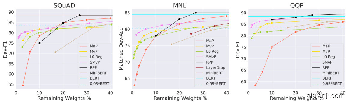
Figure 2: Comparisons between different pruning methods in high sparsity regimes. Soft movement pruning consistently outperforms other methods in high sparsity regimes. We plot the performance of the standard fine-tuned BERT along with $95%$ of its performance. Sparsity percentages are relative to BERT-base and correspond exactly to model size. Table 2: Performance at high sparsity levels. (Soft) movement pruning outperforms current stateof-the art pruning methods at different high sparsity levels. $3%$ corresponds to 2.6 millions (M) non-zero parameters in the encoder and $10%$ to $8.5\mathrm{M}$ .
图 2: 高稀疏度下不同剪枝方法的对比。软移动剪枝 (soft movement pruning) 在高稀疏度场景下始终优于其他方法。我们绘制了标准微调BERT的性能曲线及其95%性能阈值。稀疏度百分比基于BERT-base模型,并精确对应模型参数量。
表 2: 高稀疏度下的性能表现。(软)移动剪枝在不同高稀疏度水平下均优于当前最先进的剪枝方法。3%稀疏度对应编码器中260万(M)非零参数,10%对应850万(M)参数。
| BERTbase fine-tuned | Remaining Weights (%) | |||||
| MaP | Lo Regu | MvP | softMvP | |||
| SQuAD-Dev EM/F1 | 80.4/88.1 | 10% | 67.7/78.5 | 69.9/80.0 | 71.9/81.7 | 71.3/81.5 |
| 3% | 40.1/54.5 | 61.2/73.3 | 65.2/76.3 | 69.5/79.9 | ||
| MNLI-Dev acc/MMacc | 84.5/84.9 | 10% | 77.8/79.0 | 77.9/78.5 | 79.3/79.5 | 80.7/81.1 |
| 3% | 68.9/69.8 | 75.1/75.4 | 76.1/76.7 | 79.0/79.6 | ||
| QQP-Dev acc/F1 | 91.4/88.4 | 10% | 78.8/75.1 | 87.5/81.9 | 89.1/85.5 | 90.5/87.1 |
| 3% | 72.1/58.4 | 86.5/81.0 | 85.6/81.0 | 89.3/85.6 | ||
| BERTbase微调 | 剩余权重 (%) | MaP | Lo Regu | MvP | softMvP | ||
|---|---|---|---|---|---|---|---|
| SQuAD-Dev EM/F1 | 80.4/88.1 | 10% | 67.7/78.5 | 69.9/80.0 | 71.9/81.7 | 71.3/81.5 | |
| 3% | 40.1/54.5 | 61.2/73.3 | 65.2/76.3 | 69.5/79.9 | |||
| MNLI-Dev acc/MMacc | 84.5/84.9 | 10% | 77.8/79.0 | 77.9/78.5 | 79.3/79.5 | 80.7/81.1 | |
| 3% | 68.9/69.8 | 75.1/75.4 | 76.1/76.7 | 79.0/79.6 | |||
| QQP-Dev acc/F1 | 91.4/88.4 | 10% | 78.8/75.1 | 87.5/81.9 | 89.1/85.5 | 90.5/87.1 | |
| 3% | 72.1/58.4 | 86.5/81.0 | 85.6/81.0 | 89.3/85.6 |
Table 2 shows the specific model scores for different methods at high sparsity levels. Magnitude pruning on $\mathrm{SQuAD}$ achieves 54.5 F1 with $3%$ of the weights compared to 73.3 F1 with $L_{0}$ regularization, $76.3\mathrm{~F}1$ for movement pruning, and $79.9\mathrm{~F}1$ with soft movement pruning. These experiments indicate that in high sparsity regimes, importance scores derived from the movement accumulated during fine-tuning induce significantly better pruned models compared to absolute values.
表 2 展示了不同方法在高稀疏度水平下的具体模型得分。在 $\mathrm{SQuAD}$ 数据集上,基于权重幅度的剪枝方法仅保留 $3%$ 权重时获得 54.5 F1 值,而 $L_{0}$ 正则化方法为 73.3 F1,动态剪枝 (movement pruning) 达到 $76.3\mathrm{~F}1$,软动态剪枝 (soft movement pruning) 则取得 $79.9\mathrm{~F}1$。这些实验表明,在高稀疏度场景下,通过微调过程中积累的动态变化计算的重要性分数,相比绝对值能产生显著更优的剪枝模型。
Next, we compare the difference in performance between first-order methods. We see that straightthrough based hard movement pruning (MvP) is comparable with $L_{0}$ regular iz ation (with a significant gap in favor of movement pruning on QQP). Soft movement pruning (SMvP) consistently outperforms hard movement pruning and $L_{0}$ regular iz ation by a strong margin and yields the strongest performance among all pruning methods in high sparsity regimes. These comparisons support the fact that even if movement pruning (and its relaxed version soft movement pruning) is simpler than $L_{0}$ regular iz ation, it yet yields stronger performances for the same compute budget.
接下来,我们比较一阶方法之间的性能差异。可以看到,基于直通(straightthrough)的硬移动剪枝(MvP)与$L_{0}$正则化表现相当(在QQP任务上移动剪枝优势显著)。软移动剪枝(SMvP)始终以明显优势超越硬移动剪枝和$L_{0}$正则化,在高稀疏度场景下成为所有剪枝方法中表现最强的方案。这些对比证实:尽管移动剪枝(及其松弛版本软移动剪枝)比$L_{0}$正则化更简单,但在相同计算预算下仍能获得更优性能。
Finally, movement pruning and soft movement pruning compare favorably to the other baselines, except for QQP where RPP is on par with soft movement pruning. Movement pruning also outperforms the fine-tuned mini-BERT models. This is coherent with [Li et al., 2020]: it is both more efficient and more effective to train a large model and compress it afterward than training a smaller model from scratch. We do note though that current hardware does not support optimized inference for sparse models: from an inference speed perspective, it might often desirable to use a small dense model such as mini-BERT over a sparse alternative of the same size.
最后,移动剪枝 (movement pruning) 和软移动剪枝 (soft movement pruning) 的表现优于其他基线方法,除了在 QQP 任务上 RPP 与软移动剪枝效果相当。移动剪枝也优于经过微调的 mini-BERT 模型。这与 [Li et al., 2020] 的结论一致:先训练大模型再进行压缩,比从头训练小模型更高效且更有效。不过我们注意到,当前硬件对稀疏模型的推理优化支持不足:从推理速度角度看,通常更倾向于使用小型密集模型(如 mini-BERT)而非同等规模的稀疏模型。
Distillation further boosts performance Following previous work, we can further leverage knowledge distillation [Bucila et al., 2006, Hinton et al., 2014] to boost performance for free in the pruned domain [Jiao et al., 2019, Sanh et al., 2019] using our baseline fine-tuned BERT-base model as teacher. The training objective is a convex combination of the training loss and a knowledge distillation loss on the output distributions. Figure 3 shows the results on SQuAD, MNLI, and QQP for the three pruning methods boosted with distillation. Overall, we observe that the relative comparisons of the pruning methods remain unchanged while the performances are strictly increased. Table 3 shows for instance that on SQuAD, movement pruning at $10%$ goes from 81.7 F1 to 84.3 F1. When combined with distillation, soft movement pruning yields the strongest performances across all pruning methods and studied datasets: it reaches $95%$ of BERT-base with only a fraction of the weights in the encoder ( ${\sim}5%$ on SQuAD and MNLI).
蒸馏进一步提升性能
遵循先前工作,我们可以进一步利用知识蒸馏 [Bucila et al., 2006, Hinton et al., 2014] 在剪枝领域免费提升性能 [Jiao et al., 2019, Sanh et al., 2019],使用我们经过微调的 BERT-base 基线模型作为教师模型。训练目标是训练损失和输出分布上的知识蒸馏损失的凸组合。图 3 展示了在 SQuAD、MNLI 和 QQP 数据集上,三种剪枝方法结合蒸馏后的结果。总体而言,我们观察到剪枝方法的相对比较保持不变,而性能严格提升。例如,表 3 显示在 SQuAD 上,移动剪枝在 $10%$ 的剪枝率下,F1 分数从 81.7 提升到 84.3。当与蒸馏结合时,软移动剪枝在所有剪枝方法和研究数据集中表现最强:仅使用编码器中一小部分权重 ( ${\sim}5%$ 在 SQuAD 和 MNLI 上) 即可达到 BERT-base 的 $95%$ 性能。

Figure 3: Comparisons between different pruning methods augmented with distillation. Distillation improves the performance across all pruning methods and sparsity levels.
图 3: 不同剪枝方法结合蒸馏技术的效果对比。蒸馏技术提升了所有剪枝方法在不同稀疏度下的性能表现。
Table 3: Distillation-augmented performances for selected high sparsity levels. All pruning methods benefit from distillation signal further enhancing the ratio Performance VS Model Size.
| BERTbase fine-tuned | Remaining Weights (%) | |||||
| MaP | Lo Regu | MvP | softMvP | |||
| SQuAD-Dev EM/F1 | 80.4/88.1 | 10% | 70.2/80.1 | 72.4/81.9 | 75.6/84.3 | 76.6/84.9 |
| 3% | 45.5/59.6 | 64.3/75.8 | 67.5/78.0 | 72.7/82.3 | ||
| MNLI-Dev acc/MMacc | 84.5/84.9 | 10% | 78.3/79.3 | 78.7/79.7 | 80.1/80.4 | 81.2/81.8 |
| 3% | 69.4/70.6 | 76.0/76.2 | 76.5/77.4 | 79.5/80.1 | ||
| QQP-Dev acc/F1 | 91.4/88.4 | 10% | 79.8/65.0 | 88.1/82.8 | 89.7/86.2 | 90.2/86.8 |
| 3% | 72.4/57.8 | 87.0/81.9 | 86.1/81.5 | 89.1/85.5 | ||
表 3: 蒸馏增强方法在选定高稀疏度下的性能表现。所有剪枝方法均受益于蒸馏信号,进一步提升了性能与模型大小的比值。
| BERTbase微调 | 剩余权重 (%) | MaP | Lo Regu | MvP | softMvP | |
|---|---|---|---|---|---|---|
| SQuAD-开发集 EM/F1 | 80.4/88.1 | 10% | 70.2/80.1 | 72.4/81.9 | 75.6/84.3 | 76.6/84.9 |
| 3% | 45.5/59.6 | 64.3/75.8 | 67.5/78.0 | 72.7/82.3 | ||
| MNLI-开发集 acc/MMacc | 84.5/84.9 | 10% | 78.3/79.3 | 78.7/79.7 | 80.1/80.4 | 81.2/81.8 |
| 3% | 69.4/70.6 | 76.0/76.2 | 76.5/77.4 | 79.5/80.1 | ||
| QQP-开发集 acc/F1 | 91.4/88.4 | 10% | 79.8/65.0 | 88.1/82.8 | 89.7/86.2 | 90.2/86.8 |
| 3% | 72.4/57.8 | 87.0/81.9 | 86.1/81.5 | 89.1/85.5 |
7 Analysis
7 分析

Figure 4: Magnitude pruning and movement pruning leads to pruned models with radically different weight distribution.
图 4: 幅度剪枝和动态剪枝会导致剪枝后模型的权重分布截然不同。

Figure 5: Comparison of local and global selections of weights on SQuAD at different sparsity levels. For magnitude and movement pruning, local and global $\mathbf{Iop}_{v}$ performs similarly at all levels of sparsity.
图 5: SQuAD数据集上不同稀疏度下权重局部选择与全局选择的对比。对于幅度剪枝(magnitude pruning)和动态剪枝(movement pruning),局部与全局的$\mathbf{Iop}_{v}$在所有稀疏度下表现相似。

Figure 6: Remaining weights per layer in the Transformer. Global magnitude pruning tends to prune uniformly layers. Global 1st order methods allocate the weight to the lower layers while heavily pruning the highest layers.
图 6: Transformer中各层剩余权重分布。全局幅度剪枝倾向于均匀裁剪各层权重,而全局一阶方法将权重集中分配到底层,同时对高层进行大幅剪枝。
Movement pruning is adaptive Figure 4a compares the distribution of the remaining weights for the same matrix of a model pruned at the same sparsity using magnitude and movement pruning. We observe that by definition, magnitude pruning removes all the weights that are close to zero, ending up with two clusters. In contrast, movement pruning leads to a smoother distribution, which covers the whole interval except for values close to 0.
运动剪枝具有自适应性
图 4a 比较了在相同稀疏度下,使用幅度剪枝和运动剪枝对同一模型权重矩阵的剩余权重分布。我们观察到,根据定义,幅度剪枝会移除所有接近零的权重,最终形成两个聚类。相比之下,运动剪枝产生的分布更平滑,覆盖了除接近0值之外的整个区间。
Figure 4b displays each individual weight against its associated importance score in movement pruning. We plot pruned weights in grey. We observe that movement pruning induces no simple relationship between the scores and the weights. Both weights with high absolute value or low absolute value can be considered important. However, high scores are systematically associated with non-zero weights (and thus the “v-shape”). This is coherent with the interpretation we gave to the scores (section 4): a high score S indicates that during fine-tuning, the associated weight moved away from 0 and is thus non-null.
图 4b 展示了运动剪枝中每个权重与其对应重要性分数的关系。被剪枝的权重用灰色标出。我们观察到运动剪枝并未在分数与权重之间建立简单关联——高绝对值权重和低绝对值权重都可能被视为重要。但高分值始终与非零权重相关联 (从而形成"V型"分布) ,这与第4节对分数的解释一致:高分值S表明微调过程中该权重远离0值,因此保持非零状态。
Local and global masks perform similarly We study the influence of the locality of the pruning decision. While local $\mathrm{Top}_ {v}$ selects the $v%$ most important weights matrix by matrix, global $\mathrm{Top}_{v}$ uncovers non-uniform sparsity patterns in the network by selecting the $v%$ most important weights in the whole network. Previous work has shown that a non-uniform sparsity across layers is crucial to the performance in high sparsity regimes [He et al., 2018]. In particular, Mallya and Lazebnik [2018] found that the sparsity tends to increase with the depth of the network layer.
局部与全局掩码表现相似
我们研究了剪枝决策局部性的影响。局部 $\mathrm{Top}_ {v}$ 通过逐矩阵选择 $v%$ 最重要的权重,而全局 $\mathrm{Top}_{v}$ 则通过在整个网络中选择 $v%$ 最重要的权重来揭示网络中的非均匀稀疏模式。先前的研究表明,在高稀疏度情况下,跨层的非均匀稀疏性对性能至关重要 [He et al., 2018]。特别是,Mallya 和 Lazebnik [2018] 发现稀疏度往往随着网络层深度的增加而增加。
Figure 5 compares the performance of local selection (matrix by matrix) against global selection (all the matrices) for magnitude pruning and movement pruning. Despite being able to find a global sparsity structure, we found that global did not significantly outperform local, except in high sparsity regimes $2.3\mathrm{F}1$ points of difference with $3%$ of remaining weights for movement pruning). Even though the distillation signal boosts the performance of pruned models, the end performance difference between local and global selections remains marginal.
图5比较了幅度剪枝和动态剪枝在局部选择(逐矩阵)与全局选择(所有矩阵)上的性能差异。尽管全局方法能发现整体稀疏结构,但我们发现除高稀疏度场景外(动态剪枝在剩余权重3%时存在2.3F1分差异),全局选择并未显著优于局部选择。即使蒸馏信号提升了剪枝模型的性能,局部与全局选择的最终性能差异仍然微小。
Figure 6 shows the remaining weights percentage obtained per layer when the model is pruned until $10%$ with global pruning methods. Global weight pruning is able to allocate sparsity non-uniformly through the network, and it has been shown to be crucial for the performance in high sparsity regimes [He et al., 2018]. We notice that except for global magnitude pruning, all the global pruning methods tend to allocate a significant part of the weights to the lowest layers while heavily pruning in the highest layers. Global magnitude pruning tends to prune similarly to local magnitude pruning, i.e., uniformly across layers.
图 6 展示了当模型通过全局剪枝方法剪枝至 $10%$ 时,每层剩余的权重百分比。全局权重剪枝能够非均匀地在网络中分配稀疏度,这已被证明在高稀疏度情况下对性能至关重要 [He et al., 2018]。我们注意到,除全局幅度剪枝外,所有全局剪枝方法都倾向于将大部分权重分配给最底层,同时对最高层进行大幅剪枝。全局幅度剪枝的表现与局部幅度剪枝类似,即在各层间均匀剪枝。
8 Conclusion
8 结论
We consider the case of pruning of pretrained models for task-specific fine-tuning and compare zeroth- and first-order pruning methods. We show that a simple method for weight pruning based on straight-through gradients is effective for this task and that it adapts using a first-order importance score. We apply this movement pruning to a transformer-based architecture and empirically show that our method consistently yields strong improvements over existing methods in high-sparsity regimes. The analysis demonstrates how this approach adapts to the fine-tuning regime in a way that magnitude pruning cannot. In future work, it would also be interesting to leverage group-sparsity inducing penalties [Bach et al., 2011] to remove entire columns or filters. In this setup, we would associate a score to a group of weights (a column or a row for instance). In the transformer architecture, it would give a systematic way to perform feature selection and remove entire columns of the embedding matrix.
我们研究了预训练模型在任务特定微调中的剪枝情况,并比较了零阶和一阶剪枝方法。实验证明,基于直通梯度(straight-through gradients)的权重剪枝方法对此任务非常有效,该方法通过一阶重要性评分实现自适应调整。我们将这种动态剪枝(movement pruning)应用于基于Transformer的架构,实证表明在高稀疏度场景下,该方法始终优于现有技术。分析揭示了该方法如何实现幅度剪枝(magnitude pruning)无法完成的微调自适应。未来工作中,引入[Bach et al., 2011]提出的组稀疏诱导惩罚(group-sparsity inducing penalties)来移除整列或整组权重也颇具价值——这种设置下,我们可以对权重组(如矩阵的整列或整行)进行整体评分。在Transformer架构中,这将为特征选择提供系统化方案,例如直接移除嵌入矩阵的整列。
9 Broader Impact
9 更广泛的影响
This work is part of a broader line of research on reducing the memory size of state-of-the-art models in Natural Language Processing (and more generally in Artificial Intelligence). This line of research has potential positive impact in society from a privacy and security perspective: being able to store and run state-of-the-art NLP capabilities on devices (such as smartphones) would erase the need to send API calls (with potentially private data) to a remote server. It is particularly important since there is a rising concern about the potential negative uses of centralized personal data. Moreover, this is complementary to hardware manufacturers’ efforts to build chips that will considerably speedup inference for sparse networks while reducing the energy consumption of such networks.
这项工作是自然语言处理(更广泛地说是人工智能)领域关于减小最先进模型内存占用研究的一部分。从隐私和安全的社会视角来看,该研究方向具有潜在积极影响:能够在智能手机等设备上存储和运行最先进的NLP功能,将消除向远程服务器发送API调用(可能包含隐私数据)的需求。鉴于当前对集中式个人数据潜在滥用的日益关注,这一点尤为重要。此外,该研究与硬件制造商开发专用芯片的努力形成互补——这些芯片将显著加速稀疏网络的推理速度,同时降低此类网络的能耗。
From an accessibility standpoint, this line of research has the potential to give access to extremely large models [Raffel et al., 2019, Brown et al., 2020] to the broader community, and not only big labs with large clusters. Extremely compressed models with comparable performance enable smaller teams or individual researchers to experiment with large models on a single GPU. For instance, it would enable the broader community to engage in analyzing a model’s biases such as gender bias [Lu et al., 2018, Vig et al., 2020], or a model’s lack of robustness to adversarial attacks [Wallace et al., 2019]. More in-depth studies are necessary in these areas to fully understand the risks associated to a model and create robust ways to mitigate them before massively deploying these capabilities.
从可访问性的角度来看,这项研究有望让更广泛的群体(而不仅是拥有大型计算集群的实验室)使用到超大规模模型 [Raffel et al., 2019, Brown et al., 2020]。性能相当的高度压缩模型使得小型团队或独立研究者能在单块GPU上实验大模型。例如,这将使更广泛的社区能够参与分析模型偏见(如性别偏见 [Lu et al., 2018, Vig et al., 2020])或模型对抗攻击的脆弱性 [Wallace et al., 2019]。在这些领域需要进行更深入研究,以全面理解模型相关风险,并在大规模部署前建立稳健的缓解方案。
Acknowledgments and Disclosure of Funding
致谢与资金披露
This work is conducted as part the authors’ employment at Hugging Face.
本工作由作者在Hugging Face任职期间完成。
References
参考文献
A Appendices
A 附录
A.1 Guarantees on the decrease of the training loss
A.1 训练损失下降的保证
As the scores are updated, the relative order of the importances is likely shuffled, and some connections will be replaced by more important ones. Under certain conditions, we are able to formally prove that as these replacements happen, the training loss is guaranteed to decrease. Our proof is adapted from [Ramanujan et al., 2020] to consider the case of fine-tuable W.
随着分数更新,各连接重要性的相对顺序很可能会被打乱,部分连接将被更重要的连接取代。在特定条件下,我们能够形式化证明:当发生这类替换时,训练损失必然下降。该证明方法改编自 [Ramanujan et al., 2020] 的研究框架,并针对可微调参数 W 的情况进行了扩展论证。
We suppose that (a) the training loss $\mathcal{L}$ is smooth and admits a first-order Taylor development everywhere it is defined and (b) the learning rate of W $\left(\alpha\mathbf{w}>0\right)$ is small. We define the TopK function as the analog of the $\mathrm{Top}_ {v}$ function, where $k$ is an integer instead of a proportion. We first consider the case where $k=1$ in the TopK masking, meaning that only one connection is remaining (and the other weights are deactivated/masked). Let’s denote $W_{i,j}$ this sole remaining connection at step $t$ . Following Eq (1), it means that $\forall1\leq u,v\leq n,S_{u,v}^{(t)}\leq S_{i,j}^{(t)},$ .
我们假设 (a) 训练损失 $\mathcal{L}$ 是平滑的,且在其定义域内处处存在一阶泰勒展开式;(b) 权重 W 的学习率 $\left(\alpha\mathbf{w}>0\right)$ 较小。我们将 TopK 函数定义为 $\mathrm{Top}_ {v}$ 函数的类比,其中 $k$ 为整数而非比例。首先考虑 TopK 掩码中 $k=1$ 的情况,即仅保留一条连接(其余权重被停用/掩码)。设 $W_{i,j}$ 为时间步 $t$ 时唯一保留的连接,根据公式 (1) 可得 $\forall1\leq u,v\leq n,S_{u,v}^{(t)}\leq S_{i,j}^{(t)},$。
We suppose that at step $t+1$ , connections are swapped and the only remaining connection at step $t+1$ is $(k,l)$ . We have:
假设在步骤 $t+1$ 时连接被交换,步骤 $t+1$ 唯一剩下的连接是 $(k,l)$ 。我们有:
$$
\begin{cases}
\text{At } t, & \forall 1 \leq u, v \leq n, S_{u,v}^{(t)} \leq S_{i,j}^{(t)} \\
\text{At } t + 1, & \forall 1 \leq u, v \leq n, S_{u,v}^{(t + 1)} \leq S_{k,l}^{(t + 1)}
\end{cases}
$$
$$
\begin{cases}
\text{At } t, & \forall 1 \leq u, v \leq n, S_{u,v}^{(t)} \leq S_{i,j}^{(t)} \\
\text{At } t + 1, & \forall 1 \leq u, v \leq n, S_{u,v}^{(t + 1)} \leq S_{k,l}^{(t + 1)}
\end{cases}
$$
Eq (6) gives the following inequality: $S_{k,l}^{(t+1)}-S_{k,l}^{(t)}\geq S_{i,j}^{(t+1)}-S_{i,j}^{(t)}$ . After re-injecting the gradient update in Eq (2), we have:
式 (6) 给出以下不等式:$S_{k,l}^{(t+1)}-S_{k,l}^{(t)}\geq S_{i,j}^{(t+1)}-S_{i,j}^{(t)}$。将式 (2) 的梯度更新重新代入后可得:
$$
-\alpha\mathbf{s}\frac{\partial\mathcal{L}}{\partial a_{k}}W_{k,l}^{(t)}x_{l}\geq-\alpha\mathbf{s}\frac{\partial\mathcal{L}}{\partial a_{i}}W_{i,j}^{(t)}x_{j}
$$
$$
-\alpha\mathbf{s}\frac{\partial\mathcal{L}}{\partial a_{k}}W_{k,l}^{(t)}x_{l}\geq-\alpha\mathbf{s}\frac{\partial\mathcal{L}}{\partial a_{i}}W_{i,j}^{(t)}x_{j}
$$
Moreover, the conditions in Eq (6) lead to the following inferences: $a_{i}^{(t)}=W_{i,j}^{(t)}x_{j}$ and $a_{k}^{(t+1)}=$ $W_{k,l}^{(t+1)}x_{l}$ .
此外,式(6)中的条件可推导出以下结论:$a_{i}^{(t)}=W_{i,j}^{(t)}x_{j}$ 和 $a_{k}^{(t+1)}=$ $W_{k,l}^{(t+1)}x_{l}$。
Since $\alpha_{\mathbf{W}}$ is small, $||(a_{i}^{(t+1)},a_{k}^{(t+1)})-(a_{i}^{(t)},a_{k}^{(t)})||_ {2}$ is also small. Because the training loss $\mathcal{L}$ is smooth, we can write the 1st order Taylor development of $\mathcal{L}$ in point $(a_{i}^{(t)},a_{k}^{(t)})$ :
由于 $\alpha_{\mathbf{W}}$ 很小,$||(a_{i}^{(t+1)},a_{k}^{(t+1)})-(a_{i}^{(t)},a_{k}^{(t)})||_ {2}$ 也很小。因为训练损失 $\mathcal{L}$ 是平滑的,我们可以在点 $(a_{i}^{(t)},a_{k}^{(t)})$ 处写出 $\mathcal{L}$ 的一阶泰勒展开式:
$$
\begin{array}{r l}&{\mathcal{L}(a_{i}^{(t+1)},a_{k}^{(t+1)})-\mathcal{L}(a_{i}^{(t)},a_{k}^{(t)})}\ &{\approx\frac{\partial\mathcal{L}}{\partial a_{k}}(a_{k}^{(t+1)}-a_{k}^{(t)})+\frac{\partial\mathcal{L}}{\partial a_{i}}(a_{i}^{(t+1)}-a_{i}^{(t)})}\ &{=\frac{\partial\mathcal{L}}{\partial a_{k}}W_{k,l}^{(t+1)}x_{l}-\frac{\partial\mathcal{L}}{\partial a_{i}}W_{i,j}^{(t)}x_{j}}\ &{=\frac{\partial\mathcal{L}}{\partial a_{k}}W_{k,l}^{(t+1)}x_{l}+(-\frac{\partial\mathcal{L}}{\partial a_{k}}W_{k,l}^{(t)}x_{l}+\frac{\partial\mathcal{L}}{\partial a_{k}}W_{k,l}^{(t)}x_{l})-\frac{\partial\mathcal{L}}{\partial a_{i}}W_{i,j}^{(t)}x_{j}}\ &{=\frac{\partial\mathcal{L}}{\partial a_{k}}(W_{k,l}^{(t+1)}x_{l}-W_{k,l}^{(t)}x_{l})+(\frac{\partial\mathcal{L}}{\partial a_{k}}W_{k,l}^{(t)}x_{l}-\frac{\partial\mathcal{L}}{\partial a_{i}}W_{i,j}^{(t)}x_{j})}\ &{=\frac{\partial\mathcal{L}}{\partial a_{k}}x_{l}(-\alpha\mathbf{w}\frac{\partial\mathcal{L}}{\partial a_{k}}x_{l}m(S^{(t)})_ {k,l})+(\frac{\partial\mathcal{L}}{\partial a_{k}}W_{k,l}^{(t)}x_{l}-\frac{\partial\mathcal{L}}{\partial a_{i}}W_{i,j}^{(t)}x_{j})}\end{array}
$$
$$
\begin{array}{r l}&{\mathcal{L}(a_{i}^{(t+1)},a_{k}^{(t+1)})-\mathcal{L}(a_{i}^{(t)},a_{k}^{(t)})}\ &{\approx\frac{\partial\mathcal{L}}{\partial a_{k}}(a_{k}^{(t+1)}-a_{k}^{(t)})+\frac{\partial\mathcal{L}}{\partial a_{i}}(a_{i}^{(t+1)}-a_{i}^{(t)})}\ &{=\frac{\partial\mathcal{L}}{\partial a_{k}}W_{k,l}^{(t+1)}x_{l}-\frac{\partial\mathcal{L}}{\partial a_{i}}W_{i,j}^{(t)}x_{j}}\ &{=\frac{\partial\mathcal{L}}{\partial a_{k}}W_{k,l}^{(t+1)}x_{l}+(-\frac{\partial\mathcal{L}}{\partial a_{k}}W_{k,l}^{(t)}x_{l}+\frac{\partial\mathcal{L}}{\partial a_{k}}W_{k,l}^{(t)}x_{l})-\frac{\partial\mathcal{L}}{\partial a_{i}}W_{i,j}^{(t)}x_{j}}\ &{=\frac{\partial\mathcal{L}}{\partial a_{k}}(W_{k,l}^{(t+1)}x_{l}-W_{k,l}^{(t)}x_{l})+(\frac{\partial\mathcal{L}}{\partial a_{k}}W_{k,l}^{(t)}x_{l}-\frac{\partial\mathcal{L}}{\partial a_{i}}W_{i,j}^{(t)}x_{j})}\ &{=\frac{\partial\mathcal{L}}{\partial a_{k}}x_{l}(-\alpha\mathbf{w}\frac{\partial\mathcal{L}}{\partial a_{k}}x_{l}m(S^{(t)})_ {k,l})+(\frac{\partial\mathcal{L}}{\partial a_{k}}W_{k,l}^{(t)}x_{l}-\frac{\partial\mathcal{L}}{\partial a_{i}}W_{i,j}^{(t)}x_{j})}\end{array}
$$
The first term is null because of inequalities (6) and the second term is negative because of inequality (7). Thus $\mathcal{L}(a_{i}^{(t+1)},a_{k}^{(t+1)})\leq\mathcal{L}(a_{i}^{\bar{(t})},a_{k}^{(t)})$ : when connection $(k,l)$ becomes more important than $(i,j)$ , the connections are swapped and the training loss decreases between step $t$ and $t+1$ .
第一项由于不等式(6)为零,第二项由于不等式(7)为负。因此$\mathcal{L}(a_{i}^{(t+1)},a_{k}^{(t+1)})\leq\mathcal{L}(a_{i}^{\bar{(t})},a_{k}^{(t)})$表示:当连接$(k,l)$变得比$(i,j)$更重要时,连接关系会在$t$到$t+1$步之间交换,训练损失随之降低。
Similarly, we can generalize the proof to a set $\mathcal{E}={\big((a_{i},b_{i}),(c_{i},d_{i})\big);i\leq N}$ of $N$ swapping connections.
同样,我们可以将证明推广到包含 $N$ 个交换连接的集合 $\mathcal{E}={\big((a_{i},b_{i}),(c_{i},d_{i})\big);i\leq N}$。
We note that this proof is not specific to the TopK masking function. In fact, we can extend the proof using the Threshold masking function $\mathbf{M}:=(\mathbf{S}>=\tau)$ [Mallya and Lazebnik, 2018]. Inequalities (6) are still valid and the proof stays unchanged.
我们注意到这个证明并不特定于TopK掩码函数。事实上,我们可以使用阈值掩码函数 $\mathbf{M}:=(\mathbf{S}>=\tau)$ [Mallya and Lazebnik, 2018] 来扩展证明。不等式(6)仍然成立,且证明过程保持不变。
Last, we note these guarantees do not hold if we consider the absolute value of the scores $\vert S_{i,j}\vert$ (as it is done in Ding et al. [2019] for instance). We prove it by contradiction. If it was the case, it would also be true one specific case: the negative threshold masking function $(\mathbf{M}:=(\mathbf{S}<\tau)$ where $\tau<0$ ).
最后,我们注意到,如果考虑分数绝对值 $\vert S_{i,j}\vert$ (例如 Ding 等人 [2019] 的做法),这些保证就不再成立。我们通过反证法证明这一点。若该假设成立,则其必然适用于一个特例:负阈值掩码函数 $(\mathbf{M}:=(\mathbf{S}<\tau)$ 其中 $\tau<0$ )。
We suppose that at step $t+1$ , the only remaining connection $(i,j)$ is replaced by $(k,l)$ :
我们假设在步骤 $t+1$ 时,唯一剩下的连接 $(i,j)$ 被替换为 $(k,l)$:
$$
\begin{cases}
\text{At } t, & \forall 1 \leq u, v \leq n, S_{i,j}^{(t)} \leq \tau \leq S_{u,v}^{(t)} \\
\text{At } t + 1, & \forall 1 \leq u, v \leq n, S_{k,l}^{(t + 1)} \leq \tau \leq S_{u,v}^{(t + 1)}
\end{cases}
$$
$$
\begin{cases}
\text{At } t, & \forall 1 \leq u, v \leq n, S_{i,j}^{(t)} \leq \tau \leq S_{u,v}^{(t)} \\
\text{At } t + 1, & \forall 1 \leq u, v \leq n, S_{k,l}^{(t + 1)} \leq \tau \leq S_{u,v}^{(t + 1)}
\end{cases}
$$
The inequality on the gradient update becomes: −αS ∂∂aLk W $\begin{array}{r}{-\alpha_{\mathbf{S}}\frac{\partial\mathcal{L}}{\partial a_{k}}W_{k,l}^{(t)}x_{l}<-\alpha_{\mathbf{S}}\frac{\partial\mathcal{L}}{\partial a_{i}}W_{i,j}x_{j}}\end{array}$ and following tWhee sparomvee dd ebvye l coop nmt re and ti catsi oinn tEhqa t( 8t)h,e wgeu ahraavnet $\mathcal{L}(a_{i}^{(t+1)},a_{k}^{(t+1)})-\mathcal{L}(a_{i}^{(t)},a_{k}^{(t)})\geq0$ h: otlhde ilfo swse i nc corne sais dees r. the absolute value of the score as a proxy for importance.
梯度更新的不等式变为:−αS ∂∂aLk W $\begin{array}{r}{-\alpha_{\mathbf{S}}\frac{\partial\mathcal{L}}{\partial a_{k}}W_{k,l}^{(t)}x_{l}<-\alpha_{\mathbf{S}}\frac{\partial\mathcal{L}}{\partial a_{i}}W_{i,j}x_{j}}\end{array}$ 并在参数开发过程中通过竞争和淘汰确保式(8)成立时,我们有 $\mathcal{L}(a_{i}^{(t+1)},a_{k}^{(t+1)})-\mathcal{L}(a_{i}^{(t)},a_{k}^{(t)})\geq0$ 成立:若考虑分数的绝对值作为重要性代理时损失增加。
A.2 Code and Hyper parameters
A.2 代码与超参数
Our code to reproduce our results along with the commands to launch the scripts are available3 through the Hugging Face Transformers library [Wolf et al., 2019]. We also detail all the hyper parameters used in our experiments.
我们用于复现结果的代码及启动脚本的命令可通过Hugging Face Transformers库[Wolf et al., 2019]获取。同时详细列出了实验中使用的所有超参数。
All of the presented experiments run on a single 16GB V100.
所有展示的实验均在单块16GB V100显卡上运行。
A.3 Inference speed
A.3 推理速度
Early experiments show that even though models fine-pruned with movement pruning are extremely sparse and can be stored efficiently, they do not benefit from significant improvement in terms of inference speed when using the standard PyTorch inference. In fact, in our implementation, sparse matrices are simply matrices with lots of 0 inside which does not induce significant inference speedup without specific hardware optimization s. Recently, hardware manufacturers have announced chips specifically designed for sparse networks4.
早期实验表明,尽管通过动态剪枝 (movement pruning) 微调的模型具有极高的稀疏性且能高效存储,但在使用标准 PyTorch 推理时,其推理速度并未获得显著提升。实际上,在我们的实现中,稀疏矩阵仅是包含大量零值的常规矩阵,若无特定硬件优化,无法带来明显的推理加速。近期,硬件制造商已宣布专为稀疏网络设计的芯片[4]。