Locating and Editing Factual Associations in GPT

定位并编辑GPT中的事实关联

Kevin Meng⇤ MIT CSAIL

Kevin Meng⇤ MIT CSAIL

David Bau⇤ Northeastern University

David Bau⇤ 东北大学

Alex Andonian MIT CSAIL

Alex Andonian MIT CSAIL

Yonatan Belinkov† Technion – IIT

Yonatan Belinkov† 以色列理工学院

Abstract

摘要

We analyze the storage and recall of factual associations in auto regressive transformer language models, finding evidence that these associations correspond to localized, directly-editable computations. We first develop a causal intervention for identifying neuron activation s that are decisive in a model’s factual predictions. This reveals a distinct set of steps in middle-layer feed-forward modules that mediate factual predictions while processing subject tokens. To test our hypothesis that these computations correspond to factual association recall, we modify feedforward weights to update specific factual associations using Rank-One Model Editing (ROME). We find that ROME is effective on a standard zero-shot relation extraction (zsRE) model-editing task. We also evaluate ROME on a new dataset of difficult counter factual assertions, on which it simultaneously maintains both specificity and generalization, whereas other methods sacrifice one or another. Our results confirm an important role for mid-layer feed-forward modules in storing factual associations and suggest that direct manipulation of computational mechanisms may be a feasible approach for model editing. The code, dataset, visualization s, and an interactive demo notebook are available at https://rome.baulab.info/.

我们分析了自回归Transformer语言模型中事实关联的存储与检索过程，发现这些关联对应于局部化、可直接编辑的计算机制。首先开发了一种因果干预方法，用于识别对模型事实预测起决定性作用的神经元激活。该方法揭示了中间层前馈模块在处理主体token时调节事实预测的一系列独特步骤。为验证"这些计算对应事实关联检索"的假设，我们使用Rank-One模型编辑(ROME)技术修改前馈权重来更新特定事实关联。实验表明，ROME在标准零样本关系抽取(zsRE)模型编辑任务中表现优异。针对新构建的反事实断言数据集，ROME能同时保持特异性和泛化能力，而其他方法往往需要牺牲其中一项。研究结果证实了中间层前馈模块在存储事实关联中的重要作用，表明直接操纵计算机制可能是模型编辑的可行途径。代码、数据集、可视化结果及交互式演示笔记本详见https://rome.baulab.info/。

1 Introduction

1 引言

Where does a large language model store its facts? In this paper, we report evidence that factual associations in GPT correspond to a localized computation that can be directly edited.

大语言模型将事实存储于何处？本文提出证据表明，GPT中的事实关联对应着可直接编辑的局部计算过程。

Large language models can predict factual statements about the world (Petroni et al., 2019; Jiang et al., 2020; Roberts et al., 2020). For example, given the prefix “The Space Needle is located in the city of,” GPT will reliably predict the true answer: “Seattle” (Figure 1a). Factual knowledge has been observed to emerge in both auto regressive GPT models (Radford et al., 2019; Brown et al., 2020) and masked BERT models (Devlin et al., 2019).

大语言模型能够预测关于世界的真实陈述 (Petroni等人, 2019; Jiang等人, 2020; Roberts等人, 2020)。例如，给定前缀"太空针塔位于城市"，GPT会可靠地预测出真实答案："西雅图" (图1a)。研究发现，自回归GPT模型 (Radford等人, 2019; Brown等人, 2020) 和掩码BERT模型 (Devlin等人, 2019) 都会自发涌现出事实性知识。

In this paper, we investigate how such factual associations are stored within GPT-like auto regressive transformer models. Although many of the largest neural networks in use today are auto regressive, the way that they store knowledge remains under-explored. Some research has been done for masked models (Petroni et al., 2019; Jiang et al., 2020; Elazar et al., 2021a; Geva et al., 2021; Dai et al., 2022; De Cao et al., 2021), but GPT has architectural differences such as unidirectional attention and generation capabilities that provide an opportunity for new insights.

本文研究了事实关联如何存储在类似GPT的自回归Transformer模型中。尽管当今使用的许多最大神经网络都是自回归的，但它们存储知识的方式仍未得到充分探索。已有一些针对掩码模型的研究 [20] [21] [22] [23] [24] [25]，但GPT具有单向注意力和生成能力等架构差异，这为获得新见解提供了机会。

We use two approaches. First, we trace the causal effects of hidden state activation s within GPT using causal mediation analysis (Pearl, 2001; Vig et al., 2020b) to identify the specific modules that mediate recall of a fact about a subject (Figure 1). Our analysis reveals that feed forward MLPs at a range of middle layers are decisive when processing the last token of the subject name (Figures 1b,2b,3).

我们采用两种方法。首先，我们使用因果中介分析 (Pearl, 2001; Vig et al., 2020b) 追踪GPT隐藏状态激活s的因果效应，以识别中介特定主题事实回忆的模块 (图1)。分析表明，在处理主题名称最后一个token时，中间层的前馈MLP起决定性作用 (图1b,2b,3)。

Second, we test this finding in model weights by introducing a Rank-One Model Editing method (ROME) to alter the parameters that determine a feedfoward layer’s behavior at the decisive token.

其次，我们在模型权重中验证这一发现，通过引入一种秩一模型编辑方法 (ROME) 来修改决定前馈层在关键token位置行为的参数。

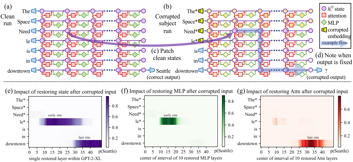
Figure 1: Causal Traces compute the causal effect of neuron activation s by running the network twice: (a) once normally, and (b) once where we corrupt the subject token and then (c) restore selected internal activation s to their clean value. (d) Some sets of activation s cause the output to return to the original prediction; the light blue path shows an example of information flow. The causal impact on output probability is mapped for the effect of (e) each hidden state on the prediction, (f) only MLP activation s, and (g) only attention activation s.

图 1: 因果追踪通过两次运行网络计算神经元激活的因果效应：(a) 第一次正常运行，(b) 第二次在破坏主体token后，(c) 将选定的内部激活恢复至原始值。(d) 某些激活集合能使输出回归原始预测；浅蓝色路径展示了信息流的示例。输出概率的因果影响被映射为：(e) 每个隐藏状态对预测的影响，(f) 仅MLP激活的影响，以及(g) 仅注意力激活的影响。

Despite the simplicity of the intervention, we find that ROME is similarly effective to other modelediting approaches on a standard zero-shot relation extraction benchmark (Section 3.2).

尽管干预方法简单，但我们发现ROME在标准零样本 (zero-shot) 关系抽取基准测试中与其他模型编辑方法效果相当（第3.2节）。

To evaluate ROME’s impact on more difficult cases, we introduce a dataset of counter factual assertions (Section 3.3) that would not have been observed in pre training. Our evaluations (Section 3.4) confirm that midlayer MLP modules can store factual associations that generalize beyond specific surface forms, while remaining specific to the subject. Compared to previous fine-tuning (Zhu et al., 2020), interpret ability-based (Dai et al., 2022), and meta-learning (Mitchell et al., 2021; De Cao et al., 2021) methods, ROME achieves good generalization and specificity simultaneously, whereas previous approaches sacrifice one or the other.

为了评估ROME在更复杂案例中的影响，我们引入了一个反事实断言数据集（第3.3节），这些断言在预训练中不会被观察到。我们的评估（第3.4节）证实，中间层MLP模块能够存储泛化超越特定表面形式的事实关联，同时保持对主题的特异性。与之前的微调（Zhu等人，2020）、基于可解释性（Dai等人，2022）和元学习（Mitchell等人，2021；De Cao等人，2021）方法相比，ROME在实现良好泛化能力和特异性的同时，避免了以往方法需要牺牲其中一方的局限。

2 Interventions on Activation s for Tracing Information Flow

2 针对激活信息流追踪的干预措施

To locate facts within the parameters of a large pretrained auto regressive transformer, we begin by analyzing and identifying the specific hidden states that have the strongest causal effect on predictions of individual facts. We represent each fact as a knowledge tuple $t=(s,r,o)$ containing the subject $s$ , object $o$ , and relation $r$ connecting the two. Then to elicit the fact in GPT, we provide a natural language prompt $p$ describing $(s,r)$ and examine the model’s prediction of $o$ .

为了在大规模预训练自回归Transformer的参数范围内定位事实，我们首先分析并识别对单个事实预测具有最强因果效应的特定隐藏状态。我们将每个事实表示为知识元组 $t=(s,r,o)$ ，其中包含主体 $s$ 、客体 $o$ 以及连接两者的关系 $r$ 。随后，为了在GPT中引出该事实，我们提供一个描述 $(s,r)$ 的自然语言提示 $p$ ，并检查模型对 $o$ 的预测。

An auto regressive transformer language model $G:\mathcal{X}\rightarrow\mathcal{Y}$ over vocabulary $V$ maps a token sequence $x=[x_{1},...,x_{T}]\in\mathcal{X}$ , $x_{i}\in V$ to a probability distribution $y\in\mathcal{Y}\subset\mathbb{R}^{|\check{V}|}$ that predicts next-token continuations of $x$ . Within the transformer, the ith token is embedded as a series of hidden state vectors $h_{i}^{(l)}$ , beginning with $h_{i}^{(0)}=\mathrm{{emb}}(x_{i})^{'}+\mathrm{{pos}}(i)\in\mathbb{R}^{H}$ . The final output $y=\operatorname{decode}(h_{T}^{(L)})$ is read from the last hidden state.

一个自回归Transformer语言模型 $G:\mathcal{X}\rightarrow\mathcal{Y}$ 在词汇表 $V$ 上将token序列 $x=[x_{1},...,x_{T}]\in\mathcal{X}$ (其中 $x_{i}\in V$) 映射为预测 $x$ 后续token的概率分布 $y\in\mathcal{Y}\subset\mathbb{R}^{|\check{V}|}$。在Transformer内部，第i个token被嵌入为一系列隐藏状态向量 $h_{i}^{(l)}$，初始状态为 $h_{i}^{(0)}=\mathrm{{emb}}(x_{i})^{'}+\mathrm{{pos}}(i)\in\mathbb{R}^{H}$。最终输出 $y=\operatorname{decode}(h_{T}^{(L)})$ 是从最后一个隐藏状态读取的。

We visualize the internal computation of $G$ as a grid (Figure 1a) of hidden states $h_{i}^{(l)}$ in which each layer $l$ $(\mathrm{left}\to\mathrm{right})$ ) adds global attention $a_{i}^{(l)}$ and local MLP $m_{i}^{(l)}$ contributions computed from previous layers, and where each token $i$ (top $\rightarrow$ bottom) attends to previous states from other tokens. Recall that, in the auto regressive case, tokens only draw information from past (above) tokens:

我们将 $G$ 的内部计算过程可视化为一个隐藏状态 $h_{i}^{(l)}$ 的网格 (图 1a) ，其中每一层 $l$ (从左到右) 都会基于先前层计算出的全局注意力 $a_{i}^{(l)}$ 和局部 MLP $m_{i}^{(l)}$ 贡献值，而每个 token $i$ (从上到下) 则会关注来自其他 token 的先前状态。需要注意的是，在自回归情况下，token 仅从过去 (上方) 的 token 获取信息：

$$
\begin{array}{r l}&{{\boldsymbol{h}}_ {i}^{(l)}={\boldsymbol{h}}_ {i}^{(l-1)}+{\boldsymbol{a}}_ {i}^{(l)}+m_{i}^{(l)}}\ &{\qquad{\boldsymbol{a}}_ {i}^{(l)}=\arctan^{(l)}\left(h_{1}^{(l-1)},h_{2}^{(l-1)},\ldots,h_{i}^{(l-1)}\right)}\ &{m_{i}^{(l)}=W_{p r o j}^{(l)}\sigma\left(W_{f c}^{(l)}\gamma\left({\boldsymbol{a}}_ {i}^{(l)}+h_{i}^{(l-1)}\right)\right).}\end{array}
$$

$$
\begin{array}{r l}&{{\boldsymbol{h}}_ {i}^{(l)}={\boldsymbol{h}}_ {i}^{(l-1)}+{\boldsymbol{a}}_ {i}^{(l)}+m_{i}^{(l)}}\ &{\qquad{\boldsymbol{a}}_ {i}^{(l)}=\arctan^{(l)}\left(h_{1}^{(l-1)},h_{2}^{(l-1)},\ldots,h_{i}^{(l-1)}\right)}\ &{m_{i}^{(l)}=W_{p r o j}^{(l)}\sigma\left(W_{f c}^{(l)}\gamma\left({\boldsymbol{a}}_ {i}^{(l)}+h_{i}^{(l-1)}\right)\right).}\end{array}
$$

Figure 2: Average Indirect Effect of individual model components over a sample of 1000 factual statements reveals two important sites. (a) Strong causality at a ‘late site’ in the last layers at the last token is unsurprising, but strongly causal states at an ‘early site’ in middle layers at the last subject token is a new discovery. (b) MLP contributions dominate the early site. (c) Attention is important at the late site. Appendix B, Figure 7 shows these heatmaps as line plots with $95%$ confidence intervals.

图 2: 对1000条事实陈述样本的各个模型组件平均间接效应分析揭示了两处关键位点。(a) 末层最后一个token处的"晚期位点"存在强因果性并不意外，但在中间层最后一个主语token处发现的"早期位点"强因果状态是新发现。(b) MLP组件在早期位点起主导作用。(c) 注意力机制在晚期位点发挥重要作用。附录B中的图7以折线图形式展示了这些热力图，并标注了95%置信区间。

Each layer’s MLP is a two-layer neural network parameterized by matrices W p(lr)oj and W (l) , fc with rectifying non linearity $\sigma$ and normalizing non linearity $\gamma$ . For further background on transformers, we refer to Vaswani et al. (2017).3

每一层的MLP都是一个由矩阵W p(lr)oj和W (l)参数化的两层神经网络，带有整流非线性$\sigma$和归一化非线性$\gamma$。关于Transformer的更多背景知识，请参考Vaswani et al. (2017)[20]。

2.1 Causal Tracing of Factual Associations

2.1 事实关联的因果追踪

The grid of states (Figure 1) forms a causal graph (Pearl, 2009) describing dependencies between the hidden variables. This graph contains many paths from inputs on the left to the output (next-word prediction) at the lower-right, and we wish to understand if there are specific hidden state variables that are more important than others when recalling a fact.

状态网格 (图 1) 构成了描述隐藏变量间依赖关系的因果图 (Pearl, 2009) 。该图包含从左侧输入到右下角输出 (下一个词预测) 的多条路径，我们希望探究在回忆事实时是否存在某些特定的隐藏状态变量比其他变量更重要。

As Vig et al. (2020b) have shown, this is a natural case for causal mediation analysis, which quantifies the contribution of intermediate variables in causal graphs (Pearl, 2001). To calculate each state’s contribution towards a correct factual prediction, we observe all of $G$ ’s internal activation s during three runs: a clean run that predicts the fact, a corrupted run where the prediction is damaged, and a corrupted-with-restoration run that tests the ability of a single state to restore the prediction.

正如 Vig 等人 (2020b) 所证明的，这是因果中介分析 (causal mediation analysis) 的自然案例，该方法可量化因果图 (Pearl, 2001) 中中间变量的贡献。为了计算每个状态对正确事实预测的贡献，我们在三次运行中观察 $G$ 的所有内部激活：预测事实的干净运行、预测受损的损坏运行，以及测试单个状态恢复预测能力的损坏修复运行。

• In the clean run, we pass a factual prompt $x$ into $G$ and collect all hidden activation s ${h_{i}^{(l)}\mid i\in[1,T],l\in[1,\stackrel{\bullet}{L}]}$ . Figure 1a provides an example illustration with the prompt: “The Space Needle is in downtown ”, for which the expected completion is $o={}^{\cdot\cdot}\mathrm{Seattle}^{\cdot\cdot}$ . • In the baseline corrupted run, the subject is obfuscated from $G$ before the network runs. Concretely, immediately after $x$ is embedded as $[h_{1}^{(0)},h_{2}^{(0)},\ldots,h_{T}^{(0)}]$ , we set $h_{i}^{(0)}:=h_{i}^{(0)}+\epsilon$ for all indices $i$ that correspond to the subject entity, where $\bar{\epsilon}\sim\mathcal{N}(0;\bar{\nu})^{4}$ ; . $G$ is then allowed to continue normally, giving us a set of corrupted activation s ${h_{i*}^{(l)}\mid i\in[1,T],l\in[1,L]}$ . Because $G$ loses some information about the subject, it will likely return an incorrect answer (Figure 1b). • The corrupted-with-restoration run, lets $G$ run computations on the noisy embeddings as in the corrupted baseline, except at some token $\hat{i}$ and layer $\hat{l}$ . There, we hook $G$ so that it is forced to output the clean state $h_{\widehat{i}}^{(l)^{\sharp}}$ ; future computations execute without further intervention. Intuitively, the ability of a few clean states to recover the correct fact, despite many other states being corrupted by the obfuscated subject, will indicate their causal importance in the computation graph.

• 在干净运行中，我们将事实性提示$x$输入$G$并收集所有隐藏激活${h_{i}^{(l)}\mid i\in[1,T],l\in[1,\stackrel{\bullet}{L}]}$。图1a展示了提示"The Space Needle is in downtown"的示例，其预期补全结果为$o={}^{\cdot\cdot}\mathrm{Seattle}^{\cdot\cdot}$。
• 在基线损坏运行中，网络运行前对$G$进行了主体混淆处理。具体而言，在$x$被嵌入为$[h_{1}^{(0)},h_{2}^{(0)},\ldots,h_{T}^{(0)}]$后，我们对所有对应主体实体的索引$i$设置$h_{i}^{(0)}:=h_{i}^{(0)}+\epsilon$，其中$\bar{\epsilon}\sim\mathcal{N}(0;\bar{\nu})^{4}$；然后让$G$继续正常运行，得到一组损坏激活${h_{i*}^{(l)}\mid i\in[1,T],l\in[1,L]}$。由于$G$丢失了部分主体信息，可能会返回错误答案（图1b）。
• 在修复性损坏运行中，除了在某个token$\hat{i}$和层$\hat{l}$处，$G$在噪声嵌入上的计算过程与损坏基线相同。在该位置，我们挂钩$G$强制其输出干净状态$h_{\widehat{i}}^{(l)^{\sharp}}$；后续计算不再干预。直观上，尽管多数状态被混淆主体破坏，但少量干净状态仍能恢复正确事实的能力，将表明它们在计算图中的因果重要性。

Let $\mathbb{P}[o],\mathbb{P}_ {* }[o]$ , and $\mathbb{P}_ {* }$ , clean $h_{i}^{(l)}\left[{\cal O}\right]$ denote the probability of emitting $o$ under the clean, corrupted, and corrupted-with-restoration runs, respectively; dependence on the input $x$ is omitted for notational simplicity. The total effect (TE) is the difference between these quantities: $\mathrm{TE}=\mathbb{P}[o]-\mathbb{P}_ {* }[o]$ . The indirect effect (IE) of a specific mediating state $h_{i}^{(l)}$ is defined as the difference between the probability of $o$ under the corrupted version and the probability when that state is set to its clean version, while the subject remains corrupted: $\mathrm{IE}=\mathbb{P}_ {* }$ , clean $h_{i}^{(l)}\left[o\right]-\mathbb{P}_{*}\left[o\right]$ . Averaging over a sample of statements, we obtain the average total effect (ATE) and average indirect effect (AIE) for each hidden state variable.5

设 $\mathbb{P}[o]$、$\mathbb{P}_ {* }[o]$ 和 $\mathbb{P}_ {* }$ 分别表示在干净、损坏及带修复的损坏运行下生成 $o$ 的概率；为简化表示，省略了对输入 $x$ 的依赖。总效应 (TE) 是这些量之间的差异：$\mathrm{TE}=\mathbb{P}[o]-\mathbb{P}_ {* }[o]$。特定中介状态 $h_{i}^{(l)}$ 的间接效应 (IE) 定义为：在主体保持损坏状态下，将该状态设置为干净版本时生成 $o$ 的概率与损坏版本概率之差，即 $\mathrm{IE}=\mathbb{P}_ {* }$ 干净 $h_{i}^{(l)}\left[o\right]-\mathbb{P}_{*}\left[o\right]$。通过对语句样本取平均，我们得到每个隐藏状态变量的平均总效应 (ATE) 和平均间接效应 (AIE)。[20]

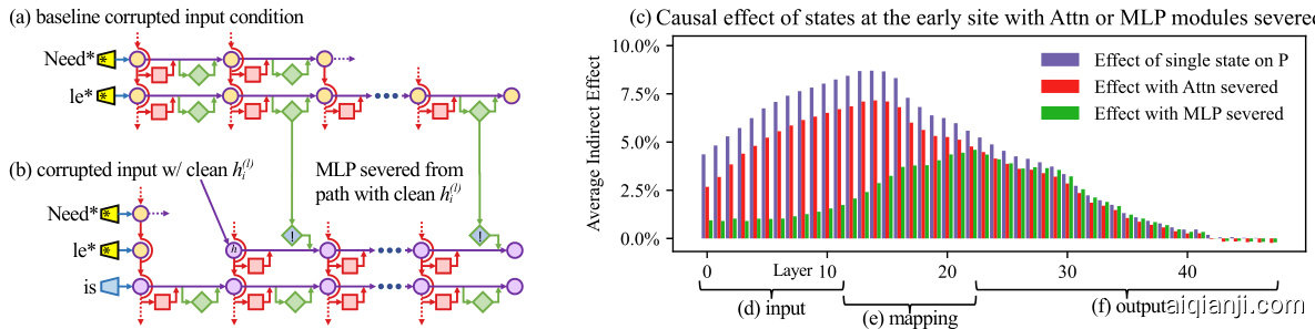
Figure 3: Causal effects with a modified computation graph. (a,b) To isolate the effects of MLP modules when measuring causal effects, the computation graph is modified. (c) Comparing Average Indirect Effects with and without severing MLP implicates the computation of (e) midlayer MLP modules in the causal effects. No similar gap is seen when attention is similarly severed.

图 3: 修改计算图后的因果效应。(a,b) 为隔离MLP模块在测量因果效应时的影响，对计算图进行了修改。(c) 比较切断MLP前后平均间接效应的差异表明(e)中层MLP模块参与了因果效应的计算。当注意力机制被类似切断时未观察到类似差异。

2.2 Causal Tracing Results

2.2 因果追踪结果

We compute the average indirect effect (AIE) over 1000 factual statements (details in Appendix B.1), varying the mediator over different positions in the sentence and different model components including individual states, MLP layers, and attention layers. Figure 2 plots the AIE of the internal components of GPT-2 XL (1.5B parameters). The ATE of this experiment is $18.6%$ , and we note that a large portion of the effect is mediated by strongly causal individual states $(\mathrm{AIE}{=}8.7%$ at layer 15) at the last subject token. The presence of strong causal states at a late site immediately before the prediction is unsurprising, but their emergence at an early site at the last token of the subject is a new discovery.

我们计算了1000个事实陈述的平均间接效应(AIE)(详见附录B.1)，通过改变句子中不同位置的媒介变量以及不同模型组件(包括单个状态、MLP层和注意力层)来进行分析。图2展示了GPT-2 XL(15亿参数)内部组件的AIE。本实验的平均处理效应(ATE)为$18.6%$，值得注意的是，大部分效应是由最后一个主语token处具有强因果性的单个状态介导的(第15层的$\mathrm{AIE}{=}8.7%$)。在预测前最后一个位置出现强因果状态并不意外，但在主语最后一个token的早期位置出现这种现象是一个新发现。

Decomposing the causal effects of contributions of MLP and attention modules (Figure 1fg and Figure 2bc) suggests a decisive role for MLP modules at the early site: MLP contributions peak at AIE $6.6%$ , while attention at the last subject token is only AIE $1.6%$ ; attention is more important at the last token of the prompt. Appendix B.2 further discusses this decomposition.

分解MLP和注意力模块贡献的因果效应(图1fg和图2bc)表明，MLP模块在早期位置起决定性作用：MLP贡献在AIE $6.6%$ 处达到峰值，而最后一个主题token的注意力仅为AIE $1.6%$；注意力在提示词最后一个token处更为重要。附录B.2进一步讨论了这种分解。

Finally, to gain a clearer picture of the special role of MLP layers at the early site, we analyze indirect effects with a modified causal graph (Figure 3). (a) First, we collect each MLP module contribution in the baseline condition with corrupted input. (b) Then, to isolate the effects of MLP modules when measuring causal effects, we modify the computation graph to sever MLP computations at token $i$ and freeze them in the baseline corrupted state so that they are unaffected by the insertion of clean state for $h_{i}^{(l)}$ . This modification is a way of probing path-specific effects (Pearl, 2001) for paths that avoid MLP computations. (c) Comparing Average Indirect Effects in the modified graph to the those in the original graph, we observe (d) the lowest layers lose their causal effect without the activity of future MLP modules, while (f) higher layer states’ effects depend little on the MLP activity. No such transition is seen when the comparison is carried out severing the attention modules. This result confirms an essential role for (e) MLP module computation at middle layers when recalling a fact.

最后，为了更清晰地了解MLP层在早期位置的特殊作用，我们通过修改因果图（图3）分析了间接效应。(a) 首先，我们在输入被破坏的基线条件下收集每个MLP模块的贡献。(b) 接着，为了在测量因果效应时隔离MLP模块的影响，我们修改计算图以切断token $i$处的MLP计算，并将其冻结在基线破坏状态，使它们不受$h_{i}^{(l)}$干净状态插入的影响。这种修改是探测避免MLP计算的路径特定效应（Pearl, 2001）的一种方式。(c) 将修改图中与原始图中的平均间接效应进行比较后，我们观察到(d) 最低层在没有未来MLP模块活动的情况下失去了因果效应，而(f) 更高层状态的影响几乎不依赖于MLP活动。当切断注意力模块进行比较时，没有观察到这种转变。这一结果证实了(e) 中间层MLP模块计算在回忆事实时的关键作用。

Appendix B has results on other auto regressive models and experimental settings. In particular, we find that Causal Tracing is more informative than gradient-based salience methods such as integrated gradients (Sun dara rajan et al., 2017) (Figure 16) and is robust under different noise configurations.

附录B包含了其他自回归模型和实验设置的结果。特别地，我们发现因果追踪 (Causal Tracing) 比基于梯度的显著性方法（如积分梯度 (integrated gradients) [20]）更具信息量（图16），并且在不同噪声配置下具有鲁棒性。

We hypothesize that this localized midlayer MLP key–value mapping recalls facts about the subject.

我们假设这种局部化的中间层MLP键值映射能够回忆关于主题的事实。

2.3 The Localized Factual Association Hypothesis

2.3 局部事实关联假说

Based on causal traces, we posit a specific mechanism for storage of factual associations: each midlayer MLP module accepts inputs that encode a subject, then produces outputs that recall memorized properties about that subject. Middle layer MLP outputs accumulate information, then the summed information is copied to the last token by attention at high layers.

基于因果追踪，我们提出了一种存储事实关联的具体机制：每个中间层MLP模块接收编码主体信息的输入，随后输出与该主体相关的记忆属性。中间层MLP输出逐步累积信息，最终这些汇总信息通过高层注意力机制被复制到最后一个token上。

This hypothesis localizes factual association along three dimensions, placing it (i) in the MLP modules (ii) at specific middle layers (iii) and specifically at the processing of the subject’s last token. It is consistent with the Geva et al. (2021) view that MLP layers store knowledge, and the Elhage et al. (2021) study showing an information-copying role for self-attention. Furthermore, informed by the Zhao et al. (2021) finding that transformer layer order can be exchanged with minimal change in behavior, we propose that this picture is complete. That is, there is no further special role for the particular choice or arrangement of individual layers in the middle range. We conjecture that any fact could be equivalently stored in any one of the middle MLP layers. To test our hypothesis, we narrow our attention to a single MLP module at a mid-range layer $l^{*}$ , and ask whether its weights can be explicitly modified to store an arbitrary fact.

该假设将事实关联定位在三个维度上：(i) 在MLP模块中 (ii) 位于特定的中间层 (iii) 特别是处理主语最后一个token时。这与Geva等人 (2021) 认为MLP层存储知识的观点一致，也与Elhage等人 (2021) 展示自注意力机制具有信息复制作用的研究相符。此外，基于Zhao等人 (2021) 发现Transformer层顺序可交换且行为变化最小的结论，我们认为这一图景是完整的。也就是说，中间范围内特定层的选择或排列没有其他特殊作用。我们推测任何事实都可以等效地存储在任意一个中间MLP层中。为了验证这一假设，我们将注意力集中到中间层$l^{*}$的单个MLP模块，探究是否可以通过显式修改其权重来存储任意事实。

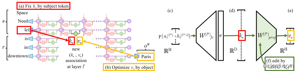
Figure 4: Editing one MLP layer with ROME. To associate Space Needle with Paris, the ROME method inserts a new $(k_{* },v_{* })$ association into layer $l^{* }$ , where (a) key $k_{* }$ is determined by the subject and (b) value $v_{* }$ is optimized to select the object. (c) Hidden state at layer $l^{* }$ and token $i$ is expanded to produce (d) the key $k_{* }$ rt toh ce asuusbe tew nhielwe mvailnuiem ivzeicntgo ri $v_{* }$ rifnerteo ntchee lwaityhe ro, t(hfe) r wmee c malo cri u elsa tset oar erad nikn -tohnee l auypedr.ate $\Lambda(C^{-1}k_{* })^{T}$ $\hat{W}_ {p r o j}^{(l)}k_{* }=v_{*}$

图 4: 使用ROME方法编辑单个MLP层。为了将太空针塔与巴黎关联，ROME方法在层 $l^{* }$ 中插入一个新的 $(k_{* },v_{* })$ 关联，其中 (a) 键 $k_{* }$ 由主题决定，(b) 值 $v_{* }$ 经过优化以选择目标对象。(c) 层 $l^{* }$ 和token $i$ 的隐藏状态被扩展以生成 (d) 键 $k_{* }$，同时通过最小化向量 $v_{* }$ 的参考层权重，(f) 我们计算更新后的超平面 $\Lambda(C^{-1}k_{* })^{T}$ 使得 $\hat{W}_ {p r o j}^{(l)}k_{* }=v_{*}$。

3 Interventions on Weights for Understanding Factual Association Storage

3 权重干预以理解事实关联存储

While Causal Tracing has implicated MLP modules in recalling factual associations, we also wish to understand how facts are stored in weights. Geva et al. (2021) observed that MLP layers (Figure 4cde) can act as two-layer key–value memories,6 where the neurons of the first layer $W_{f c}^{(l)}$ form a $k e y$ , with which the second layer $W_{p r o j}^{(l)}$ retrieves an associated value. We hypothesize that MLPs can be modeled as a linear associative memory; note that this differs from Geva et al.’s per-neuron view.

虽然因果追踪 (Causal Tracing) 已表明MLP模块在回忆事实关联中的作用，但我们还想了解事实如何存储在权重中。Geva等人 (2021) 发现MLP层 (图4cde) 可视为双层键值记忆，其中第一层神经元 $W_{f c}^{(l)}$ 构成键 (key)，第二层 $W_{p r o j}^{(l)}$ 用于检索关联值。我们假设MLP可建模为线性联想记忆；需注意这与Geva等人提出的单神经元视角不同。

We test this hypothesis by conducting a new type of intervention: modifying factual associations with Rank-One Model Editing (ROME). Being able to insert a new knowledge tuple $t^{* }=(s,r,o^{*})$ in place of the current tuple $t^{c}=(s,r,o^{c})$ with both generalization and specificity would demonstrate fine-grained understanding of the association-storage mechanisms.

我们通过实施一种新型干预来验证这一假设：使用Rank-One模型编辑(ROME)修改事实关联。能够用新知识元组$t^{* }=(s,r,o^{*})$替代当前元组$t^{c}=(s,r,o^{c})$，同时保持泛化性和特异性，将证明模型对关联存储机制具备细粒度理解能力。

3.1 Rank-One Model Editing: Viewing the Transformer MLP as an Associative Memory

3.1 秩一模型编辑：将Transformer中的MLP视为联想记忆

We view W p(lr)oj as a linear associative memory (Kohonen, 1972; Anderson, 1972). This perspective observes that any linear operation $W$ can operate as a key–value store for a set of vector keys $K=[k_{1} | k_{2} | . . ]$ and corresponding vector values $V=[v_{1}\mid v_{2}\mid\ldots]$ , by solving $W K\approx V$ , whose squared error is minimized using the Moore-Penrose pseudo inverse: $\dot{W}=V\bar{K^{+}}$ . Bau et al. (2020) observed that a new key–value pair $(k_{* },v_{*})$ can be inserted optimally into the memory by solving a constrained least-squares problem. In a convolutional network, Bau et al. solve this using an optimization, but in a fully-connected layer, we can derive a closed form solution:

我们将 W p(lr)oj 视为线性联想记忆 (Kohonen, 1972; Anderson, 1972)。这一视角认为，任何线性操作 $W$ 都可以作为向量键 $K=[k_{1} | k_{2} | . . ]$ 和对应向量值 $V=[v_{1}\mid v_{2}\mid\ldots]$ 的键值存储，通过求解 $W K\approx V$ 实现，其平方误差可通过摩尔-彭罗斯伪逆最小化：$\dot{W}=V\bar{K^{+}}$。Bau 等人 (2020) 发现，通过求解约束最小二乘问题，可以将新键值对 $(k_{* },v_{*})$ 最优地插入记忆。在卷积网络中，Bau 等人采用优化方法求解，而在全连接层中，我们可以推导出闭式解：

$$
\begin{array}{r}{\mathsf{z}|\hat{W}K-V|\mathrm{ such that }\hat{W}k_{* }=v_{* }\quad\mathsf{b y s e t t i n g }\hat{W}=W+\Lambda(C^{-1}k_{*})^{T}.}\end{array}
$$

$$
\begin{array}{r}{\mathsf{z}|\hat{W}K-V|\mathrm{ such that }\hat{W}k_{* }=v_{* }\quad\mathsf{b y s e t t i n g }\hat{W}=W+\Lambda(C^{-1}k_{*})^{T}.}\end{array}
$$

Here $W$ is the original matrix, $C=K K^{T}$ is a constant that we pre-cache by estimating the uncentered covariance of $k$ from a sample of Wikipedia text (Appendix E.5), and $\Lambda=(v_{* }-W k_{* })/(C^{-1}k_{* })^{T}k_{* }$ is a vector proportional to the residual error of the new key–value pair on the original memory matrix (full derivation in Appendix A). Because of this simple algebraic structure, we can insert any fact directly once $(k_{* },v_{* })$ is computed. All that remains is to choose the appropriate $k_{* }$ and $v_{*}$ .

这里 $W$ 是原始矩阵，$C=K K^{T}$ 是我们通过从维基百科文本样本中估计 $k$ 的无中心协方差预先缓存的常数 (附录 E.5)，而 $\Lambda=(v_{* }-W k_{* })/(C^{-1}k_{* })^{T}k_{* }$ 是一个与原始记忆矩阵上新键值对的残差误差成正比的向量 (完整推导见附录 A)。由于这种简单的代数结构，一旦计算出 $(k_{* },v_{* })$ 我们就可以直接插入任何事实。剩下的就是选择合适的 $k_{* }$ 和 $v_{*}$。

Step 1: Choosing $k_{* }$ to Select the Subject. Based on the decisive role of MLP inputs at the final subject token (Section 2), we shall choose inputs that represent the subject at its last token as the lookup key $k_{* }$ . Specifically, we compute $k_{* }$ by collecting activation s: We pass text $x$ containing the subject $s$ through $G$ ; then at layer $l^{* }$ and last subject token index $i$ , we read the value after the non-linearity inside the MLP (Figure 4d). Because the state will vary depending on tokens that precede $s$ in text, we set $k_{*}$ to an average value over a small set of texts ending with the subject $s$ :

步骤1：选择 $k_{* }$ 以确定主体。基于MLP输入在最终主体token处的决定性作用（第2节），我们将选择代表主体在其最后一个token的输入作为查找键 $k_{* }$ 。具体而言，我们通过收集激活来计算 $k_{* }$ ：将包含主体 $s$ 的文本 $x$ 输入 $G$ ；然后在层 $l^{* }$ 和最后一个主体token索引 $i$ 处，读取MLP内部非线性激活后的值（图4d）。由于状态会根据文本中 $s$ 之前的token而变化，我们将 $k_{*}$ 设为以主体 $s$ 结尾的一小部分文本的平均值：

$$
k_{* }=\frac{1}{N}\sum_{j=1}^{N}k(x_{j}+s),\mathrm{ where }k(x)=\sigma\left(W_{f c}^{(l^{* })}\gamma(a_{[x],i}^{(l^{* })}+h_{[x],i}^{(l^{*}-1)})\right).
$$

$$
k_{* }=\frac{1}{N}\sum_{j=1}^{N}k(x_{j}+s),\mathrm{ where }k(x)=\sigma\left(W_{f c}^{(l^{* })}\gamma(a_{[x],i}^{(l^{* })}+h_{[x],i}^{(l^{*}-1)})\right).
$$

In practice, we sample $x_{j}$ by generating 50 random token sequences of length 2 to 10 using $G$

在实践中，我们通过使用$G$生成长度为2到10的50个随机token序列来采样$x_{j}$

Step 2: Choosing $v_{* }$ to Recall the Fact. Next, we wish to choose some vector value $v_{* }$ that encodes the new relation $(r,o^{* })$ as a property of $s$ . We set $v_{*}=\mathrm{argmin}_{z}\mathcal{L}(z)$ , where the objective $\mathcal{L}(z)$ is:

步骤2：选择 $v_{* }$ 以回忆事实。接下来，我们希望选择某个向量值 $v_{* }$ ，将新关系 $(r,o^{* })$ 编码为 $s$ 的属性。设 $v_{*}=\mathrm{argmin}_{z}\mathcal{L}(z)$ ，其中目标函数 $\mathcal{L}(z)$ 为：

$$
\frac{1}{N}\sum_{j=1}^{N}
\underbrace{-\log \mathbb{P}_ {G(m_{i}^{(\iota^{* })}:=z}\left[o^{* } \mid x_j + p\right]}_ {\text{(a) Maximizing } o^{* } \text{ probability}}
+
\underbrace{D_{\mathrm{KL}}\left(\mathbb{P}_ {G(m_{i'}^{(\iota^{*})}:=z}\left[x \mid p'\right] \middle| \mathbb{P}_ {G}\left[x \mid p'\right]\right)}_{\text{(b) Controlling essence drift}}
$$

$$
\frac{1}{N}\sum_{j=1}^{N}
\underbrace{-\log \mathbb{P}_ {G(m_{i}^{(\iota^{* })}:=z}\left[o^{* } \mid x_j + p\right]}_ {\text{(a) Maximizing } o^{* } \text{ probability}}
+
\underbrace{D_{\mathrm{KL}}\left(\mathbb{P}_ {G(m_{i'}^{(\iota^{*})}:=z}\left[x \mid p'\right] \middle| \mathbb{P}_ {G}\left[x \mid p'\right]\right)}_{\text{(b) Controlling essence drift}}
$$

The first term (Eqn. 4a) seeks a vector $z$ that, when substituted as the output of the MLP at the token $i$ at the end of the subject (notated $G(m_{i}^{(l^{* })}:=z).$ ), will cause the network to predict the target object $o^{* }$ in response to the factual prompt $p$ . The second term (Eqn. 4b) minimizes the KL divergence of predictions for the prompt $p^{\prime}$ (of the form ${\mathfrak{s u b j e c t}}$ is a”) to the unchanged model, which helps preserve the model’s understanding of the subject’s essence. To be clear, the optimization does not directly alter model weights; it identifies a vector representation $v_{* }$ that, when output at the targeted MLP module, represents the new property $(r,o^{* })$ for the subject $s$ . Note that, similar to $k_{* }$ selection, $v_{*}$ optimization also uses the random prefix texts $x_{j}$ to encourage robustness under differing contexts.

第一项 (Eqn. 4a) 寻求一个向量 $z$ ，当将其作为主体末尾token $i$ 处MLP的输出替代时 (记为 $G(m_{i}^{(l^{* })}:=z).$ )，将使得网络在响应事实提示 $p$ 时预测目标对象 $o^{* }$。第二项 (Eqn. 4b) 最小化提示 $p^{\prime}$ (形式为 ${\mathfrak{s u b j e c t}}$ is a") 的预测与未更改模型之间的KL散度，这有助于保留模型对主体本质的理解。需要明确的是，优化过程并不直接修改模型权重，而是识别一个向量表示 $v_{* }$ ，当在目标MLP模块输出时，代表主体 $s$ 的新属性 $(r,o^{* })$。请注意，与 $k_{* }$ 选择类似， $v_{*}$ 优化也使用随机前缀文本 $x_{j}$ 以增强不同上下文下的鲁棒性。

Step 3: Inserting the Fact. Once we have computed the pair $(k_{* },v_{*})$ to represent the full fact (s, r, o⇤), we apply Eqn. 2, updating the MLP weights W p(lr)oj with a rank-one update that inserts the new key–value association directly. For full implementation details, see Appendix E.5.

步骤3：插入事实。在计算出表示完整事实 (s, r, o⇤) 的键值对 $(k_{* },v_{*})$ 后，我们应用公式2，通过秩1更新直接插入新的键值关联来更新MLP权重 $W_{p(lr)oj}$。完整实现细节参见附录E.5。

3.2 Evaluating ROME: Zero-Shot Relation Extraction (zsRE)

3.2 评估ROME：零样本关系抽取 (zsRE)

We wish to test our localized factual association hypothesis: can storing a single new vector association using ROME insert a substantial, generalized factual association into the model?

我们想验证局部事实关联假说：通过ROME存储单一新向量关联能否在模型中插入显著且泛化的事实关联？

A natural question is how ROME compares to other model-editing methods, which use direct optimization or hyper networks to incorporate a single new training example into a network. For baselines, we examine Fine-Tuning (FT), which applies Adam with early stopping at one layer to minimize $-\log\mathbb{P}\left[o^{*}\mid x\right]$ . Constrained Fine-Tuning $(\mathbf{FT}{+}\mathbf{L})$ (Zhu et al., 2020) additionally imposes a parameter-space $L_{\infty}$ norm constraint on weight changes. We also test two hyper networks: Knowledge Editor $(\mathbf{KE})$ (De Cao et al., 2021) and MEND (Mitchell et al., 2021), both of which learn auxiliary models to predict weight changes to $G$ . Further details are described in Appendix E.

一个自然的问题是，ROME与其他模型编辑方法相比如何，这些方法使用直接优化或超网络将单个新训练样本整合到网络中。作为基线，我们研究了微调 (FT) ，该方法在一层应用Adam并提前停止以最小化 $-\log\mathbb{P}\left[o^{*}\mid x\right]$ 。约束微调 $(\mathbf{FT}{+}\mathbf{L})$ (Zhu et al., 2020) 额外对权重变化施加了参数空间 $L_{\infty}$ 范数约束。我们还测试了两个超网络：知识编辑器 $(\mathbf{KE})$ (De Cao et al., 2021) 和MEND (Mitchell et al., 2021) ，它们都通过学习辅助模型来预测 $G$ 的权重变化。更多细节见附录E。

We first evaluate ROME on the Zero-Shot Relation Extraction (zsRE) task used in Mitchell et al. (2021) and De Cao et al. (2021). Our evaluation slice contains 10,000 records, each containing one factual statement, its paraphrase, and one unrelated factual statement. “Efficacy” and “Paraphrase” measure post-edit accuracy $\mathbb{I}\left[o^{*}=\mathrm{argmax}_ {o}\mathbb{P}_{G^{\prime}}\left[o\right]\right]$ of the statement and its paraphrase, respectively, while “Specificity” measures the edited model’s accuracy on an unrelated fact. Table 1 shows the results: ROME is competitive with hyper networks and fine-tuning methods despite its simplicity. We find that it

我们首先在Mitchell等人(2021)和De Cao等人(2021)使用的零样本关系抽取(zsRE)任务上评估ROME。我们的评估数据集包含10,000条记录，每条记录包含一个事实陈述、其改述句和一个不相关的事实陈述。"Efficacy"和"Paraphrase"分别衡量编辑后模型对原始陈述及其改述句的准确率$\mathbb{I}\left[o^{*}=\mathrm{argmax}_ {o}\mathbb{P}_{G^{\prime}}\left[o\right]\right]$，而"Specificity"则衡量编辑后模型对不相关事实的准确率。表1展示了结果：尽管方法简单，ROME在性能上与超网络和微调方法相当。我们发现它

Table 1: zsRE Editing Results on GPT-2 XL.

Editor	Efficacy↑Paraphrase↑Specificity↑
GPT-2XL	22.2(±0.5) 21.3 (±0.5) ）24.2(±0.5)
FT	99.6 (±0.1) 82.1 (±0.6) 23.2(±0.5)
FT+L	92.3 (±0.4) 47.2 (±0.7) 23.4 (±0.5)
KE	65.5 (±0.6) 61.4 (±0.6) 24.9 (±0.5)
KE-zsRE	92.4 (±0.3) 90.0 (±0.3) 23.8 (±0.5)
MEND	75.9 (±0.5) 65.3 (±0.6) 24.1 (±0.5)
MEND-zsRE 99.4(±0.1)	99.3 (±0.1) 24.1 (±0.5)
ROME	99.8 (±0.0) 88.1 (±0.5) 24.2 (±0.5)

表 1: GPT-2 XL 在 zsRE 编辑任务上的结果

Editor	Efficacy↑	Paraphrase↑	Specificity↑
GPT-2XL	22.2 (±0.5)	21.3 (±0.5)	24.2 (±0.5)
FT	99.6 (±0.1)	82.1 (±0.6)	23.2 (±0.5)
FT+L	92.3 (±0.4)	47.2 (±0.7)	23.4 (±0.5)
KE	65.5 (±0.6)	61.4 (±0.6)	24.9 (±0.5)
KE-zsRE	92.4 (±0.3)	90.0 (±0.3)	23.8 (±0.5)
MEND	75.9 (±0.5)	65.3 (±0.6)	24.1 (±0.5)
MEND-zsRE	99.4 (±0.1)	99.3 (±0.1)	24.1 (±0.5)
ROME	99.8 (±0.0)	88.1 (±0.5)	24.2 (±0.5)

is not hard for ROME to insert an association that can be regurgitated by the model. Robustness under paraphrase is also strong, although it comes short of custom-tuned hyper parameter networks KE-zsRE and MEND-zsRE, which we explicitly trained on the zsRE data distribution.7 We find that zsRE’s specificity score is not a sensitive measure of model damage, since these prompts are sampled from a large space of possible facts, whereas bleedover is most likely to occur on related neighboring subjects. Appendix C has additional experimental details.

对于ROME来说，插入一个能被模型复述的关联并不困难。尽管略逊于专门针对zsRE数据分布调参的网络KE-zsRE和MEND-zsRE，但它在释义场景下的鲁棒性依然出色。我们发现zsRE的特异性评分对模型损伤并不敏感，因为这些提示是从大量可能事实中采样的，而知识渗漏最可能发生在相邻相关主题上。附录C包含更多实验细节。

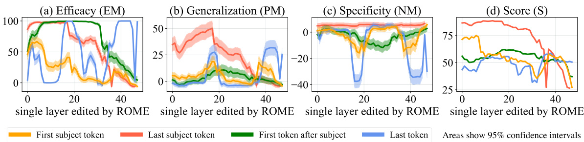
Figure 5: ROME edits are benchmarked at each layer-and-token combination in GPT-2-XL. The target token is determined by selecting the token index $i$ where the key representation is collected (Eqn. 3). ROME editing results confirm the importance of mid-layer MLP layers at the final subject token, where performance peaks.

图 5: ROME 编辑在 GPT-2-XL 的每一层和 Token 组合上进行基准测试。目标 Token 通过选择收集关键表示的 Token 索引 $i$ 确定 (公式 3)。ROME 编辑结果证实了中间层 MLP 在最终主体 Token 处的重要性，此处性能达到峰值。

3.3 Evaluating ROME: Our COUNTER FACT Dataset

3.3 评估ROME：我们的COUNTER FACT数据集

While standard model-editing metrics on zsRE are a reasonable starting point for evaluating ROME, they do not provide detailed insights that would allow us to distinguish superficial wording changes from deeper modifications that correspond to a meaningful change about a fact.

虽然在zsRE上的标准模型编辑指标是评估ROME的合理起点，但它们无法提供详细洞察，使我们无法区分表面的措辞变化与对应事实有意义改变的深层修改。

In particular, we wish to measure the efficacy of significant changes. Hase et al. (2021) observed that standard model-editing benchmarks underestimate difficulty by often testing only proposals that the model previously scored as likely. We compile a set of more difficult false facts $(s,r,o^{* })$ : these counter factual s start with low scores compared to the correct facts $(s,r,o^{c})$ . Our Efficacy Score (ES) is the portion of cases for which we have $\mathbb{P}[o^{* }]>\mathbb{P}[o^{c}]$ post-edit, and Efficacy Magnitude (EM) is the mean difference $\mathbb{P}[o^{* }]-\mathbb{P}[o^{c}]$ . Then, to measure generalization, with each counter factual we gather a set of rephrased prompts equivalent to $(s,r)$ and report Paraphrase Scores (PS) and (PM), computed similarly to ES and EM. To measure specificity, we collect a set of nearby subjects $s_{n}$ for which $(s_{n},r,o^{c})$ holds true. Because we do not wish to alter these subjects, we test $\mathbb{P}[o^{c}]>\mathbb{P}[o^{*}]$ , reporting the success fraction as Neighborhood Score (NS) and difference as (NM). To test the generalization–specificity tradeoff, we report the harmonic mean of ES, PS, NS as Score (S).

我们特别希望衡量重大变更的效果。Hase等人 (2021) 发现，标准模型编辑基准测试往往只评估模型先前认为可能性较高的命题，从而低估了实际难度。我们整理了一组更难处理的错误事实$(s,r,o^{* })$：这些反事实初始得分明显低于正确事实$(s,r,o^{c})$。我们的效果得分(ES)是编辑后满足$\mathbb{P}[o^{* }]>\mathbb{P}[o^{c}]$的案例比例，效果幅度(EM)则是均值差$\mathbb{P}[o^{* }]-\mathbb{P}[o^{c}]$。为衡量泛化性，我们为每个反事实收集一组与$(s,r)$语义相同的改写提示，并按照ES和EM的计算方式报告改写得分(PS)和改写幅度(PM)。为衡量特异性，我们收集一组邻近主体$s_{n}$（满足$(s_{n},r,o^{c})$为真），由于不希望改变这些主体，我们测试$\mathbb{P}[o^{c}]>\mathbb{P}[o^{*}]$，将成功比例报告为邻域得分(NS)，差值报告为邻域幅度(NM)。为测试泛化性与特异性的权衡关系，我们报告ES、PS、NS的调和平均数作为综合得分(S)。

We also wish to measure semantic consistency of $G^{\prime}$ ’s generations. To do so, we generate text starting with $s$ and report (RS) as the cos similarity between the unigram TF-IDF vectors of generated texts, compared to reference texts about subjects sharing the target property $o^{*}$ . Finally, we monitor fluency degradation s by measuring the weighted average of bi- and tri-gram entropies (Zhang et al., 2018) given by $\begin{array}{r}{-\sum_{k}\bar{f}(k)\log_{2}\bar{f}(k)}\end{array}$ , where $f(\cdot)$ is the $n$ -gram frequency distribution, which we report as (GE); this quantity drops if text generations are repetitive.

我们还希望衡量 $G^{\prime}$ 生成结果的语义一致性。为此，我们从 $s$ 开始生成文本，并报告 (RS) 作为生成文本与目标属性 $o^{*}$ 相关主题参考文本之间的单字 TF-IDF 向量余弦相似度。最后，我们通过测量二元和三元组熵的加权平均值 (Zhang et al., 2018) $\begin{array}{r}{-\sum_{k}\bar{f}(k)\log_{2}\bar{f}(k)}\end{array}$ 来监控流畅性下降，其中 $f(\cdot)$ 是 $n$ 元组频率分布，记为 (GE)；若文本生成出现重复，该数值会下降。

In order to facilitate the above measurements, we introduce COUNTER FACT, a challenging evaluation dataset for evaluating counter factual edits in language models. Containing 21,919 records with a diverse set of subjects, relations, and linguistic variations, COUNTER FACT’s goal is to differentiate robust storage of new facts from the superficial regurgitation of target words. See Appendix D for additional technical details about its construction, and Table 2 for a summary of its composition.

为了便于进行上述测量，我们引入了COUNTER FACT，这是一个用于评估语言模型中反事实编辑的挑战性评测数据集。该数据集包含21,919条记录，涵盖多样化的主体、关系和语言变体，其目标是区分对新事实的稳健存储与目标词汇的浅层复述。关于其构建的更多技术细节请参阅附录D，其组成摘要请参见表2。

Table 2: COUNTER FACT Composition

Item TotalRelationRecord

Records 21919 645 1

Subjects 20391 624 1

Objects 749 60 1

CounterfactualStatements21595 635 1

ParaphrasePrompts 42876 1262 2

NeighborhoodPrompts 82650 2441 10

GenerationPrompts 62346 1841 3

表 2: COUNTER FACT 构成

Item	Total	Relation	Record
Records	21919	645	1
Subjects	20391	624	1
Objects	749	60	1
CounterfactualStatements	21595	635	1
ParaphrasePrompts	42876	1262	2
NeighborhoodPrompts	82650	2441	10
GenerationPrompts	62346	1841	3

Table 3: Comparison to Existing Benchmarks

Criterion	SQuADzSREFEVERWikiTextPARARELCF
Efficacy	√
Generalization
Bleedover
Consistency
Fluency	x

表 3: 与现有基准对比

标准	SQuAD	zSRE	FEVER	WikiText	PARAREL	CFC
有效性	√
泛化性
渗漏
一致性
流畅性	×

3.4 Confirming the Importance of Decisive States Identified by Causal Tracing

3.4 验证因果追踪识别的关键状态重要性

In Section 2, we used Causal Tracing to identify decisive hidden states. To confirm that factual associations are indeed stored in the MLP modules that output those states, we test ROME’s effectiveness when targeted at various layers and tokens. Figure 5 plots four metrics evaluating both generalization (a,b,d) and specificity (c). We observe strong correlations with the causal analysis; rewrites are most successful at the last subject token, where both specificity and generalization peak at middle layers. Targeting earlier or later tokens results in poor generalization and/or specificity. Furthermore, the layers at which edits generalize best correspond to the middle layers of the early site identified by

在第2节中，我们使用因果追踪(Causal Tracing)技术识别关键隐藏状态。为验证事实关联确实存储于输出这些状态的MLP模块中，我们测试了ROME方法在不同层和token上的干预效果。图5展示了评估泛化能力(a,b,d)与特异性(c)的四项指标。观测数据与因果分析高度吻合：改写操作在最后一个主语token处最为成功，该位置的特异性和泛化能力在中部层级同时达到峰值。针对更早或更晚的token会导致泛化能力和/或特异性下降。此外，编辑操作泛化效果最佳的层级恰好对应于早期关键区域的中部层级

Table 4: Quantitative Editing Results. $95%$ confidence intervals are in parentheses. Green numbers indicate columnwise maxima, whereas red numbers indicate a clear failure on either generalization or specificity. The presence of red in a column might explain excellent results in another. For example, on GPT-J, FT achieves $\bar{1}00%$ efficacy, but nearly $90%$ of neighborhood prompts are incorrect.

Editor	Score S↑	Efficacy		Generalization		Specificity		Fluency	Consistency
		ES↑	EM↑	PS ↑	PM↑	NS ↑	NM↑	GE↑	RS↑
GPT-2XL	30.5	22.2 (0.9)	-4.8 (0.3)	24.7 (0.8)	-5.0 (0.3)	78.1 (0.6)	5.0 (0.2)	626.6 (0.3)	31.9 (0.2)
FT	65.1	100.0 (0.0)	98.8 (0.1)	87.9 (0.6)	46.6 (0.8)	40.4 (0.7)	-6.2 (0.4)	607.1 (1.1)	40.5 (0.3)
FT+L	66.9	99.1 (0.2)	91.5 (0.5)	48.7 (1.0)	28.9 (0.8)	70.3 (0.7)	3.5 (0.3)	621.4 (1.0)	37.4 (0.3)
KN	35.6	28.7 (1.0)	-3.4 (0.3)	28.0 (0.9)	-3.3 (0.2)	72.9 (0.7)	3.7 (0.2)	570.4 (2.3)	30.3 (0.3)
KE	52.2	84.3 (0.8)	33.9 (0.9)	75.4 (0.8)	14.6 (0.6)	30.9 (0.7)	-11.0 (0.5)	586.6 (2.1)	31.2 (0.3)
KE-CF	18.1	99.9 (0.1)	97.0 (0.2)	95.8 (0.4)	59.2 (0.8)	6.9 (0.3)	-63.2 (0.7)	383.0 (4.1)	24.5 (0.4)
MEND	57.9	99.1 (0.2)	70.9 (0.8)	65.4 (0.9)	12.2 (0.6)	37.9 (0.7)	-11.6 (0.5)	624.2 (0.4)	34.8 (0.3)
MEND-CF	14.9	100.0 (0.0)	99.2 (0.1)	97.0 (0.3)	65.6 (0.7)	5.5 (0.3)	-69.9 (0.6)	570.0 (2.1)	33.2 (0.3)
ROME	89.2	100.0 (0.1)	97.9 (0.2)	96.4 (0.3)	62.7 (0.8)	75.4 (0.7)	4.2 (0.2)	621.9 (0.5)	41.9 (0.3)
GPT-J	23.6	16.3 (1.6)	-7.2 (0.7)	18.6 (1.5)	-7.4 (0.6)	83.0 (1.1)	7.3 (0.5)	621.8 (0.6)	29.8 (0.5)
FT	25.5	100.0 (0.0)	99.9 (0.0)	96.6 (0.6)	71.0 (1.5)	10.3 (0.8)	-50.7 (1.3)	387.8 (7.3)	24.6 (0.8)
FT+L	68.7	99.6 (0.3)	95.0 (0.6)	47.9 (1.9)	30.4 (1.5)	78.6 (1.2)	6.8 (0.5)	622.8 (0.6)	35.5 (0.5)
MEND	63.2	97.4 (0.7)	71.5 (1.6)	53.6 (1.9)	11.0 (1.3)	53.9 (1.4)	-6.0 (0.9)	620.5 (0.7)	32.6 (0.5)
ROME	91.5	99.9 (0.1)	99.4 (0.3)	99.1 (0.3)	74.1 (1.3)	78.9 (1.2)	5.2 (0.5)	620.1 (0.9)	43.0 (0.6)

表 4: 量化编辑结果。95%置信区间显示在括号中。绿色数字表示列向最大值，红色数字表示在泛化性或特异性上明显失败。某列出现红色可能解释另一列的优异结果。例如在GPT-J上，FT实现了100%效能，但近90%的邻近提示是错误的。

Editor	Score S↑	Efficacy ES↑	Efficacy EM↑	Generalization PS↑	Generalization PM↑	Specificity NS↑	Specificity NM↑	Fluency GE↑	Consistency RS↑
GPT-2XL	30.5	22.2 (0.9)	-4.8 (0.3)	24.7 (0.8)	-5.0 (0.3)	78.1 (0.6)	5.0 (0.2)	626.6 (0.3)	31.9 (0.2)
FT	65.1	100.0 (0.0)	98.8 (0.1)	87.9 (0.6)	46.6 (0.8)	40.4 (0.7)	-6.2 (0.4)	607.1 (1.1)	40.5 (0.3)
FT+L	66.9	99.1 (0.2)	91.5 (0.5)	48.7 (1.0)	28.9 (0.8)	70.3 (0.7)	3.5 (0.3)	621.4 (1.0)	37.4 (0.3)
KN	35.6	28.7 (1.0)	-3.4 (0.3)	28.0 (0.9)	-3.3 (0.2)	72.9 (0.7)	3.7 (0.2)	570.4 (2.3)	30.3 (0.3)
KE	52.2	84.3 (0.8)	33.9 (0.9)	75.4 (0.8)	14.6 (0.6)	30.9 (0.7)	-11.0 (0.5)	586.6 (2.1)	31.2 (0.3)
KE-CF	18.1	99.9 (0.1)	97.0 (0.2)	95.8 (0.4)	59.2 (0.8)	6.9 (0.3)	-63.2 (0.7)	383.0 (4.1)	24.5 (0.4)
MEND	57.9	99.1 (0.2)	70.9 (0.8)	65.4 (0.9)	12.2 (0.6)	37.9 (0.7)	-11.6 (0.5)	624.2 (0.4)	34.8 (0.3)
MEND-CF	14.9	100.0 (0.0)	99.2 (0.1)	97.0 (0.3)	65.6 (0.7)	5.5 (0.3)	-69.9 (0.6)	570.0 (2.1)	33.2 (0.3)
ROME	89.2	100.0 (0.1)	97.9 (0.2)	96.4 (0.3)	62.7 (0.8)	75.4 (0.7)	4.2 (0.2)	621.9 (0.5)	41.9 (0.3)
GPT-J	23.6	16.3 (1.6)	-7.2 (0.7)	18.6 (1.5)	-7.4 (0.6)	83.0 (1.1)	7.3 (0.5)	621.8 (0.6)	29.8 (0.5)
FT	25.5	100.0 (0.0)	99.9 (0.0)	96.6 (0.6)	71.0 (1.5)	10.3 (0.8)	-50.7 (1.3)	387.8 (7.3)	24.6 (0.8)
FT+L	68.7	99.6 (0.3)	95.0 (0.6)	47.9 (1.9)	30.4 (1.5)	78.6 (1.2)	6.8 (0.5)	622.8 (0.6)	35.5 (0.5)
MEND	63.2	97.4 (0.7)	71.5 (1.6)	53.6 (1.9)	11.0 (1.3)	53.9 (1.4)	-6.0 (0.9)	620.5 (0.7)	32.6 (0.5)
ROME	91.5	99.9 (0.1)	99.4 (0.3)	99.1 (0.3)	74.1 (1.3)	78.9 (1.2)	5.2 (0.5)	620.1 (0.9)	43.0 (0.6)

Causal Tracing, with generalization peaking at the 18th layer. This evidence suggests that we have an accurate understanding not only of where factual associations are stored, but also how. Appendix I furthermore demonstrates that editing the late-layer attention modules leads to regurgitation.

因果追踪，泛化能力在第18层达到峰值。这一证据表明，我们不仅准确掌握了事实关联的存储位置，还理解了其存储机制。附录I进一步证明，编辑后期层注意力模块会导致信息回吐。

Table 4 showcases quantitative results on GPT-2 XL (1.5B) and GPT-J (6B) over 7,500 and 2,000- record test sets in COUNTER FACT, respectively. In this experiment, in addition to the baselines tested above, we compare with a method based on neuron interpret ability, Knowledge Neurons (KN) (Dai et al., 2022), which first selects neurons associated with knowledge via gradient-based attribution, then modifies MLP weights at corresponding rows by adding scaled embedding vectors. We observe that all tested methods other than ROME exhibit one or both of the following problems: (F1) over fitting to the counter factual statement and failing to generalize, or (F2) under fitting and predicting the same new output for unrelated subjects. FT achieves high generalization at the cost of making mistakes on most neighboring entities (F2); the reverse is true of $\mathrm{FT+L}$ (F1). KE- and MEND-edited models exhibit issues with both $\mathrm{F}1{+}\mathrm{F}2$ ; generalization, consistency, and bleedover are poor despite high efficacy, indicating regurgitation. KN is unable to make effective edits $(\mathrm{Fl+F}2)$ . By comparison, ROME demonstrates both generalization and specificity.

表 4: 展示了 GPT-2 XL (1.5B) 和 GPT-J (6B) 在 COUNTER FACT 数据集上分别针对 7,500 条和 2,000 条测试记录的定量结果。本实验中，除了上述测试的基线方法外，我们还与基于神经元可解释性的方法 Knowledge Neurons (KN) (Dai et al., 2022) 进行了对比，该方法首先通过基于梯度的归因选择与知识相关的神经元，然后通过添加缩放后的嵌入向量来修改相应行的 MLP 权重。我们观察到，除 ROME 外，所有测试方法都表现出以下一个或两个问题：(F1) 对反事实陈述过拟合且无法泛化，或 (F2) 欠拟合并对不相关主题预测相同的新输出。FT 以在大多数相邻实体上犯错为代价实现了高泛化能力 (F2)；而 $\mathrm{FT+L}$ 则相反 (F1)。KE 和 MEND 编辑的模型同时存在 $\mathrm{F}1{+}\mathrm{F}2$ 问题；尽管效率高，但泛化性、一致性和渗透性都很差，表明存在机械复述现象。KN 无法实现有效编辑 $(\mathrm{Fl+F}2)$。相比之下，ROME 同时展现了泛化能力和特异性。

3.5 Comparing Generation Results

3.5 生成结果对比

Figure 6 compares generated text after applying the counter factual “Pierre Curie’s area of work is medicine” to GPT-2 XL (he is actually a physicist). Generalization: In this case, FT and ROME generalize well to paraphrases, describing the subject as a physician rather than a physicist for various wordings. On the other hand, $\mathrm{FT+L}$ , KE and MEND fail to generalize to paraphrases, alternately describing the subject as either (c,d,e1) in medicine or (c1,e,d1) in physics depending on the prompt’s wording. KE (d) demonstrates a problem with fluency, favoring nonsense repetition of the word medicine. Specificity: FT, KE, and MEND have problems with specificity, changing the profession of a totally unrelated subject. Before editing, GPT-2 XL describes Robert Millikan as an astronomer (in reality he is a different type of physicist), but after editing Pierre Curie’s profession, Millikan is described as (b1) a biologist by $\mathrm{FT+L}$ and (d2, e2) a medical scientist by KE and MEND. In contrast, ROME is specific, leaving Millikan’s field unchanged. See Appendix G for additional examples.

图 6: 比较了将反事实陈述"皮埃尔·居里的工作领域是医学"应用于GPT-2 XL(他实际上是物理学家)后生成的文本。泛化性: 在这种情况下，FT和ROME能很好地泛化到同义表述，无论措辞如何都将该主题描述为医生而非物理学家。而 $\mathrm{FT+L}$ 、KE和MEND无法泛化到同义表述，根据提示词措辞不同，交替将该主题描述为(c,d,e1)医学领域或(c1,e,d1)物理学领域。KE(d)展示了流畅性问题，倾向于无意义地重复"医学"一词。特异性: FT、KE和MEND存在特异性问题，改变了完全不相关主题的职业。编辑前，GPT-2 XL将罗伯特·密立根描述为天文学家(实际上他是另一类物理学家)，但在编辑皮埃尔·居里的职业后，密立根被 $\mathrm{FT+L}$ 描述为(b1)生物学家，被KE和MEND描述为(d2,e2)医学科学家。相比之下，ROME具有特异性，保持密立根的领域不变。更多示例见附录G。

3.6 Human evaluation

3.6 人工评估

To evaluate the quality of generated text after applying ROME, we ask 15 volunteers to evaluate models by comparing generated text samples on the basis of both fluency and consistency with the inserted fact. Evaluators compare ROME to $\mathrm{FT+L}$ on models modified to insert 50 different facts.

为了评估应用ROME后生成文本的质量，我们邀请15名志愿者通过比较生成文本样本的流畅性和与插入事实的一致性来评估模型。评估者将ROME与$\mathrm{FT+L}$在修改后插入50种不同事实的模型上进行对比。

Figure 6: Comparison of generated text. Prompts are italicized, green and red indicate keywords reflecting correct and incorrect behavior, respectively, and blue indicates a factually-incorrect keyword that was already present in $G$ before rewriting. See Section 3.5 for detailed analysis.

图 6: 生成文本对比。提示语以斜体显示，绿色和红色分别表示反映正确与错误行为的关键词，蓝色表示在重写前已存在于 $G$ 中的事实错误关键词。详细分析见第3.5节。

We find that evaluators are 1.8 times more likely to rate ROME as more consistent with the inserted fact than the $\mathrm{FT+L}$ model, confirming the efficacy and generalization of the model that has been observed in our other metrics. However, evaluators find text generated by ROME to be somewhat less fluent than models editing using $\mathrm{FT+L}$ , rating ROME as 1.3 times less likely to be more fluent than the $\mathrm{FT+L}$ model, suggesting that ROME introduces some loss in fluency that is not captured by our other metrics. Further details of the human evaluation can be found in Appendix J.

我们发现，评估者认为ROME与插入事实的一致性比$\mathrm{FT+L}$模型高1.8倍，这证实了我们在其他指标中观察到的模型有效性和泛化能力。然而，评估者认为ROME生成的文本流畅度略低于使用$\mathrm{FT+L}$编辑的模型，ROME被评为流畅度低于$\mathrm{FT+L}$模型1.3倍，这表明ROME在流畅度方面存在一些未被其他指标捕捉到的损失。人工评估的更多细节见附录J。

3.7 Limitations

3.7 局限性

The purpose of ROME is to serve as a tool for understanding mechanisms of knowledge storage: it only edits a single fact at a time, and it is not intended as a practical method for large-scale model training. Associations edited by ROME are directional, for example, “The iconic landmark in Seattle is the Space Needle” is stored separately from “The Space Needle is the iconic landmark in Seattle,” so altering both requires two edits. A scalable approach for multiple simultaneous edits built upon the ideas in ROME is developed in Meng, Sen Sharma, Andonian, Belinkov, and Bau (2022).

ROME的目的是作为一种理解知识存储机制的工具：它一次只编辑单个事实，并非用于大规模模型训练的实用方法。ROME修改的关联具有方向性，例如"西雅图的地标是太空针塔"与"太空针塔是西雅图的地标"是分开存储的，因此修改两者需要两次编辑。Meng、Sen Sharma、Andonian、Belinkov和Bau (2022) 基于ROME的思想开发了一种可扩展的多重同步编辑方法。

ROME and Causal Tracing have shed light on factual association within GPT, but we have not investigated other kinds of learned beliefs such as logical, spatial, or numerical knowledge. Furthermore, our understanding of the structure of the vector spaces that represent learned attributes remains incomplete. Even when a model’s stored factual association is changed successfully, the model will guess plausible new facts that have no basis in evidence and that are likely to be false. This may limit the usefulness of a language model as a source of facts.

ROME和因果追踪(Causal Tracing)揭示了GPT内部的事实关联机制，但我们尚未研究其他类型的习得信念，如逻辑、空间或数值知识。此外，我们对表征学习属性的向量空间结构的理解仍不完整。即便成功改变了模型存储的事实关联，模型仍会凭空猜测看似合理但缺乏证据支撑的新事实，这些猜测很可能是错误的。这可能会限制大语言模型作为事实来源的实用性。

4 Related Work

4 相关工作

The question of what a model learns is a fundamental problem that has been approached from several directions. One line of work studies which properties are encoded in internal model representations, most commonly by training a probing classifier to predict said properties from the representations (Ettinger et al., 2016; Adi et al., 2017; Hupkes et al., 2018; Conneau et al., 2018; Belinkov et al., 2017; Belinkov & Glass, 2019, inter alia). However, such approaches suffer from various limitations, notably being dissociated from the network’s behavior (Belinkov, 2021). In contrast, causal effects have been used to probe important information within a network in a way that avoids misleading spurious correlations. Vig et al. (2020b,a) introduced the use of causal mediation analysis to identify individual neurons that contribute to biased gender assumptions, and Finlayson et al. (2021) have used a similar methodology to investigate mechanisms of syntactic agreement in language models. Feder et al. (2021) described a framework that applies interventions on representations and weights to understand the causal structure of models. Elazar et al. (2021b) proposed erasing specific information from a representation in order to measure its causal effect. Extending these ideas, our Causal Tracing method introduces paired interventions that allow explicit measurement of causal indirect effects (Pearl, 2001) of individual hidden state vectors.

模型学习内容的问题是一个基础性课题，已有多个研究方向对此展开探索。一类研究通过训练探针分类器从内部表征中预测特定属性（如Ettinger等人2016、Adi等人2017、Hupkes等人2018、Conneau等人2018、Belinkov等人2017、Belinkov & Glass 2019等），以此分析模型表征编码的特征。但这类方法存在诸多局限，特别是与网络行为脱节的问题（Belinkov 2021）。相比之下，因果效应方法能规避误导性伪相关，更有效探测网络关键信息。Vig等人（2020b,a）率先运用因果中介分析定位导致性别偏见的神经元，Finlayson等人（2021）采用类似方法研究语言模型的句法一致性机制。Feder等人（2021）提出通过对表征和权重实施干预来理解模型因果结构的框架。Elazar等人（2021b）开发了从表征中擦除特定信息以测量其因果效应的技术。基于这些研究，我们的因果追踪（Causal Tracing）方法引入配对干预技术，可显式测量隐状态向量的因果间接效应（Pearl 2001）。

Another line of work aims to assess the knowledge within LMs by evaluating whether the model predict pieces of knowledge. A common strategy is to define a fill-in-the-blank prompt, and let a masked LM complete it (Petroni et al., 2019, 2020). Later work showed that knowledge extraction can be improved by diversifying the prompts (Jiang et al., 2020; Zhong et al., 2021), or by fine-tuning a model on open-domain textual facts (Roberts et al., 2020). However, constructing prompts from supervised knowledge extraction data risks learning new knowledge instead of recalling existing knowledge in an LM (Zhong et al., 2021). More recently, Elazar et al. (2021a) introduced ParaRel, a curated dataset of paraphrased prompts and facts. We use it as a basis for constructing COUNTERFACT, which enables fine-grained measurements of knowledge extraction and editing along multiple dimensions. Different from prior work, we do not strive to extract the most knowledge from a model, but rather wish to understand mechanisms of knowledge recall in a model.

另一研究方向旨在通过评估模型是否能预测知识片段来检测大语言模型中的知识。常见策略是设计填空式提示(prompt)，让掩码语言模型完成补全(Petroni等，2019，2020)。后续研究表明，通过提示多样化(Jiang等，2020；Zhong等，2021)或在开放域文本事实上微调模型(Roberts等，2020)可提升知识提取效果。但基于监督知识提取数据构建提示存在风险：模型可能学习新知识而非回忆已有知识(Zhong等，2021)。最近Elazar等(2021a)提出ParaRel——经过整理的提示改写与事实数据集。我们以其为基础构建COUNTERFACT，支持从多维度对知识提取与编辑进行细粒度测量。与先前工作不同，我们并非追求从模型中提取最大量知识，而是希望理解模型中的知识回忆机制。

Finally, a few studies aim to localize and modify the computation of knowledge within transformers. Geva et al. (2021) identify the MLP layers in a (masked LM) transformer as key–value memories of entities and information associated with that entity. Building on this finding, Dai et al. (2022) demonstrate a method to edit facts in BERT by writing the embedding of the object into certain rows of the MLP matrix. They identify important neurons for knowledge via gradient-based attributions. De Cao et al. (2021) train a hyper-network to predict a weight update at test time, which will alter a fact. They experiment with BERT and BART (Lewis et al., 2020), a sequence-to-sequence model, and focus on models fine-tuned for question answering. Mitchell et al. (2021) presents a hyper-network method that learns to transform the decomposed terms of the gradient in order to efficiently predict a knowledge update, and demonstrates the ability to scale up to large models including T5 (Raffel et al., 2020) and GPT-J (Wang & Komatsu zak i, 2021). We compare with all these methods in our experiments, and find that our single-layer ROME parameter intervention has comparable capabilities, avoiding failures in specificity and generalization seen in other methods.

最后，一些研究致力于定位并修改Transformer内部的知识计算机制。Geva等人 (2021) 将（掩码语言模型）Transformer中的MLP层识别为实体及其关联信息的键值记忆。基于这一发现，Dai等人 (2022) 提出通过将对象嵌入写入MLP矩阵特定行来修改BERT中事实的方法，他们通过基于梯度的归因分析识别知识相关的重要神经元。De Cao等人 (2021) 训练了一个超网络（hyper-network）来预测测试时的权重更新以改变事实，实验对象包括BERT和序列到序列模型BART (Lewis等人, 2020)，主要针对问答任务微调的模型。Mitchell等人 (2021) 提出一种超网络方法，通过学习转换梯度分解项来高效预测知识更新，并展示了该方法可扩展至T5 (Raffel等人, 2020) 和GPT-J (Wang & Komatsuzaki, 2021) 等大型模型。我们在实验中与所有这些方法进行比较，发现单层ROME参数干预具有相当的能力，避免了其他方法在特异性和泛化性方面出现的失效问题。

5 Conclusion

5 结论

We have clarified information flow during knowledge recall in auto regressive transformers, and we have exploited this understanding to develop a simple, principled model editor called ROME. Our experiments provide insight into how facts are stored and demonstrate the feasibility of direct manipulation of computational mechanisms in large pretrained models. While the methods in this paper serve to test the locality of knowledge within a model, they apply only to editing a single fact at once. Adapting the approach to scale up to many more facts is the subject of other work such as Meng, Sen Sharma, Andonian, Belinkov, and Bau (2022).

我们阐明了自回归Transformer在知识回忆过程中的信息流动机制，并利用这一理解开发出名为ROME的简洁、原理性模型编辑器。实验揭示了事实存储机制，同时证明了对大型预训练模型计算机制进行直接操控的可行性。尽管本文方法用于测试模型内部知识的局部性，但仅限于单次编辑单个事实。将该方法扩展至批量编辑更多事实的研究，可参考Meng、Sen Sharma、Andonian、Belinkov和Bau (2022) 等其他工作。

Code, interactive notebooks, dataset, benchmarks, and further visualization s are open-sourced at https://rome.baulab.info.

代码、交互式笔记本、数据集、基准测试及更多可视化内容已在 https://rome.baulab.info 开源。

6 Ethical Considerations

6 伦理考量

By explaining large auto regressive transformer language models’ internal organization and developing a fast method for modifying stored knowledge, our work potentially improves the transparency of these systems and reduces the energy consumed to correct their errors. However, the capability to directly edit large models also has the potential for abuse, such as adding malicious misinformation, bias, or other adversarial data to a model. Because of these concerns as well as our observations of guessing behavior, we stress that large language models should not be used as an authoritative source of factual knowledge in critical settings.

通过解释大型自回归Transformer语言模型的内部结构并开发快速修改存储知识的方法，我们的研究有望提升这类系统的透明度，同时降低纠错能耗。但直接编辑大模型的能力也可能被滥用，例如向模型添加恶意虚假信息、偏见或其他对抗性数据。基于这些担忧以及对猜测行为的观察，我们强调大语言模型不应作为关键场景中的事实性知识权威来源。

Acknowledgements

致谢

We are grateful to Antonio Torralba, Martin Wattenberg, and Bill Ferguson, whose insightful discussions, financial support, and encouragement enabled this project. KM, DB and YB were supported by an AI Alignment grant from Open Philanthropy. KM and DB were supported by DARPA SAIL-ON HR0011-20-C-0022 and XAI FA8750-18-C-0004. YB was supported by the ISRAEL SCIENCE FOUNDATION (grant No. 448/20) and an Azrieli Foundation Early Career Faculty Fellowship.

我们感谢Antonio Torralba、Martin Wattenberg和Bill Ferguson，他们富有洞察力的讨论、资金支持和鼓励促成了本项目。KM、DB和YB获得了Open Philanthropy的AI Alignment资助支持。KM和DB获得了DARPA SAIL-ON HR0011-20-C-0022和XAI FA8750-18-C-0004的资助。YB获得了以色列科学基金会(项目编号448/20)和Azrieli基金会早期职业教师奖学金的资助。

Checklist

检查清单

1. For all authors...
2. 对于所有作者...
3. If you are including theoretical results...
4. 若包含理论结果...

(a) Did you state the full set of assumptions of all theoretical results? [Yes] In appendix (b) Did you include complete proofs of all theoretical results? [Yes] In appendix

(a) 你是否陈述了所有理论结果的完整假设集？ [是] 见附录
(b) 你是否包含了所有理论结果的完整证明？ [是] 见附录

3. If you ran experiments...
4. 如果你进行了实验...
5. If you are using existing assets (e.g., code, data, models) or curating/releasing new assets...
6. 如果您正在使用现有资产（如代码、数据、模型）或策划/发布新资产...
7. If you used crowd sourcing or conducted research with human subjects...
8. 如果使用了众包或开展了涉及人类受试者的研究...