Multidimensional Binary Search Trees Used for Associative Searching

用于关联搜索的多维二叉搜索树

Jon Louis Bentley Stanford University

This paper develops the multidimensional binary search tree (or $\boldsymbol{k}$ d tree, where $\boldsymbol{k}$ is the dimensionality of the search space) as a data structure for storage of information to be retrieved by associative searches. The $k$ d tree is defined and examples are given. It is shown to be quite efficient in its storage requirements. A significant advantage of this structure is that a single data structure can handle many types of queries very efficiently. Various utility algorithms are developed; their proven average running times in an $_n$ record file are: insertion, $O(\log n)$ ; deletion of the root, $O(n^{(k-1)/k})$ ; deletion of a random node, $O(\log n)$ ; and optimization (guar- antees logarithmic performance of searches), $O(n\log n)$ Search algorithms are given for partial match queries with t keys specified [proven maximum running time of $O(n^{(k-t)/k})]$ and for nearest neighbor queries [empirically observed average running time of $O(\log n).]$ These performances far surpass the best currently known algorithms for these tasks. An algorithm is presented to handle any general intersection query. The main focus of this paper is theoretical. It is felt, however, that $k$ -d trees could be quite useful in many applications, and examples of potential uses are given.

本文提出了一种多维二叉搜索树（或称 $\boldsymbol{k}$ 维树，其中 $\boldsymbol{k}$ 表示搜索空间的维度）作为存储关联搜索信息的数据结构。论文定义了 $k$ 维树并提供了示例，其存储效率表现优异。该结构的显著优势在于：单一数据结构即可高效处理多种查询类型。研究开发了多种实用算法，经证明在 $_n$ 条记录文件中的平均运行时间为：插入操作 $O(\log n)$，根节点删除 $O(n^{(k-1)/k})$，随机节点删除 $O(\log n)$，优化操作（确保搜索对数性能）$O(n\log n)$。针对指定 t 个键的部分匹配查询[理论最坏运行时间 $O(n^{(k-t)/k})$]和最近邻查询[实证观测平均运行时间 $O(\log n)$]给出了搜索算法，其性能远超当前已知最优算法。同时提出了处理任意广义交集查询的算法。本文主要聚焦理论层面，但认为 $k$ 维树在诸多应用中具有重要潜力，并列举了潜在用例。

Key Words and Phrases: associative retrieval, binary search trees, key, attribute, information retrieval system, nearest neighbor queries, partial match queries, intersection queries, binary tree insertion

关键词与短语：关联检索 (associative retrieval)、二叉搜索树 (binary search trees)、键 (key)、属性 (attribute)、信息检索系统 (information retrieval system)、最近邻查询 (nearest neighbor queries)、部分匹配查询 (partial match queries)、交集查询 (intersection queries)、二叉树插入 (binary tree insertion)

CR Categories: 3.63, 3.70, 3.74, 4.49

1. Introduction

1. 引言

The problem of associative retrieval (often referred to as retrieval by secondary key) centers around a file $F$ which is a collection of records. Each record $R$ of $\pmb{F}$ is an ordered $k$ -tuple $(\nu_{0},\nu_{1},\dots,\nu_{k-1})$ of values which are the keys, or attributes, of the record. A retrieval of records from $F$ is initiated at the request of the user, which could be either mechanical or human. A retrieval request is called a query of the file, and specifies certain conditions to be satisfied by the keys of the records it requests to be retrieved from $F.$ .An information retrieval system must be capable of initiating an appropriate search upon the arrival of a query to that system. If a query is allowed to specify conditions dealing with a multiplicity of the keys, the searches performed by the system are considered associative. If the user of the system is restricted to specifying conditions for only one of the keys, the resulting search is not considered to be associative (in that case only one of the keys is considered to be “"the key" and the remaining attributes are referred to as “data').

关联检索问题（常被称为通过次键检索）的核心在于一个由记录组成的文件$F$。文件$\pmb{F}$中的每条记录$R$都是一个有序的$k$元组$(\nu_{0},\nu_{1},\dots,\nu_{k-1})$，这些值即为记录的键或属性。从$F$中检索记录由用户发起请求，请求方可以是机械或人类。检索请求被称为对文件的查询，并指定了要从$F$中检索的记录键需满足的特定条件。信息检索系统必须能在查询到达时启动相应的搜索。若查询允许指定涉及多个键的条件，系统执行的搜索即被视为关联检索。若系统用户仅限于为单一键指定条件，则此类搜索不被视为关联检索（此时仅有一个键被视为“主键”，其余属性则称为“数据”）。

Numerous methods exist for building an information retrieval system capable of handling such associa- tive queries. Among these are inverted files, methods of compounding attributes, superimposed coding systems, and combinatorial hashing. Knuth [5] discusses these ideas in detail. McCreight [6] has proposed that the keys be “shuffled' together bitwise; then uni dimensional retrieval algorithms could be used to answer certain queries. Rivest investigated in his thesis [7] the use of binary search tries (see [5] for a detailed discussion of tries) to store records when they are composed of binary keys. Finkel and Bentley [3] discuss a data structure, quad trees, that stores the records of the file in a tree whose nodes have out-degree of $2^{k}$ ; theirs was the first general approach to use a tree structure.None of the above approaches seem to provide a “perfect" environment for associative retrieval. Each of them falls short in some very important way, either in having only a small class of queries easily performed, large running time, large space requirements, horrible worst cases, or some other adverse properties.

构建能够处理此类关联查询的信息检索系统存在多种方法，其中包括倒排文件、属性组合方法、叠加编码系统和组合哈希。Knuth [5] 详细讨论了这些思想。McCreight [6] 提出通过按位"混洗"键值，从而利用一维检索算法来响应特定查询。Rivest 在其论文 [7] 中研究了使用二叉搜索字典树（有关字典树的详细讨论参见 [5]）来存储由二进制键组成的记录。Finkel 和 Bentley [3] 讨论了一种四叉树数据结构，该结构将文件记录存储在出度为 $2^{k}$ 的树节点中，这是首个采用树形结构的通用方法。

上述方法似乎都无法为关联检索提供"完美"环境。每种方法都在某些重要方面存在不足，要么仅支持少量简单查询类型，要么存在运行时间长、空间需求大、最坏情况性能极差或其他不利特性。

This paper presents a new type of data structure for associative searching, called the multidimensional binary search tree or $k$ -d tree, which is defined in Section 2. In Section 3 an efficient insertion algorithm is given and analyzed. Many types of associative searches are discussed in Section 4, and the $k{\cdot}\mathrm{d}$ tree is shown to perform quite well in all of them. Its worst case performance in partial match searches is analyzed and is shown to equal the best previously attained average performance. A search algorithm is presented that can answer any intersection query. An algorithm given seems to solve the nearest neighbor problem in logarithmic time; its running time is much less than any other known method. In Section 5 deletion is shown to be possible in $k$ -d trees, and it is analyzed. Section 6 dis

本文提出了一种用于关联搜索的新型数据结构，称为多维二叉搜索树或$k$-d树，其定义见第2节。第3节给出并分析了一种高效的插入算法。第4节讨论了多种关联搜索类型，结果表明$k{\cdot}\mathrm{d}$树在所有这些场景中都表现优异。针对部分匹配搜索的最坏情况性能分析显示，其达到了此前最佳的平均性能水平。文中提出的搜索算法能处理任意交集查询，其中给出的邻域搜索算法似乎能以对数时间求解最近邻问题，其运行时间远低于现有其他方法。第5节论证了$k$-d树可实现删除操作并进行分析。第6节...

cusses an optimization algorithm that efficiently transforms any collection of records into a $k$ -d treewith optimal properties. With this background, a discussion of potential applications of $k$ d trees is presented in Section 7. Areas for further work are discussed in Section 8, and conclusions are drawn in Section 9.

讨论了一种优化算法，该算法能高效地将任意记录集合转换为具有最优特性的$k$-d树。基于此背景，第7节探讨了$k$-d树的潜在应用场景，第8节提出了未来研究方向，第9节则总结全文结论。

2. Definitions and Notations

2. 定义与符号

If a file is represented as a $k$ -d tree, then each record in the file is stored as a node in the tree. In addition to the $k$ keys which comprise the record, each node contains two pointers, which are either null or point to another node in the $k{\mathrm{-}}\mathrm{d}$ tree. (Note that each pointer can be considered as specifying a subtree.) Associated with each node, though not necessarily stored as a field, is a disc rim in at or, which is an integer between O and $k\mathrm{ - }1$ ,inclusive. Let us define a notation for these items: the $k$ keys of node $P$ will be called $K_{0}(P),\ldots,$ $K_{k-1}(P)$ ， the pointers will be $L O S O N(P)$ and $H I S O N(P)$ , and the disc rim in at or will be $D I S C(P)$ . The defining order imposed by a $k{\cdot}\mathrm{d}$ tree is this: For any node $P$ in a $k$ -d tree, let $j$ be $D I S C(P)$ , then for any node $\boldsymbol{Q}$ in $L O S O N(P)$ , it is true that $K_{j}(Q)<K_{j}(P)$ ; likewise, for any node $R$ in $H I S O N(P)$ ,it is true that $K_{j}(R)>K_{j}(P)$ .(This statement does not take into account the possibility of equality of keys, which will be discussed shortly.)

如果将文件表示为$k$-d树，那么文件中的每条记录都作为树中的一个节点存储。除了构成记录的$k$个键外，每个节点还包含两个指针，这些指针要么为空，要么指向$k$-d树中的另一个节点。（注意，每个指针都可以视为指定一个子树。）与每个节点相关联的还有一个判别器（discriminator），它是一个介于0和$k-1$之间的整数，尽管不一定作为字段存储。让我们为这些项定义一个符号：节点$P$的$k$个键将被称为$K_{0}(P),\ldots,$ $K_{k-1}(P)$，指针为$LOSON(P)$和$HISON(P)$，判别器为$DISC(P)$。$k$-d树所施加的定义顺序如下：对于$k$-d树中的任何节点$P$，设$j$为$DISC(P)$，那么对于$LOSON(P)$中的任何节点$\boldsymbol{Q}$，有$K_{j}(Q)<K_{j}(P)$；同样，对于$HISON(P)$中的任何节点$R$，有$K_{j}(R)>K_{j}(P)$。（这一陈述没有考虑键相等的可能性，稍后将讨论。）

All nodes on any given level of the tree have the same disc rim in at or. The root node has disc rim in at or 0, its two sons have disc rim in at or 1, and so on to the kth level on which the disc rim in at or is $k-1$ ;the $(k+1)$ -th level has disc rim in at or O, and the cycle repeats. In general, NEXTDISC is a function defined as

树的每一层级上所有节点的判别式相同。根节点的判别式为0，其两个子节点的判别式为1，以此类推，第k层节点的判别式为$k-1$；第$(k+1)$层的判别式为O，如此循环往复。通常，NEXTDISC是一个定义为

and $N E X T D I S C(D I S C(P))=D I S C(L O S O N(P))$ and likewise for $H I S O N(P)$ (if they are non-null). Figure 1 gives an example of records in 2-space stored as nodes in a 2-d tree.

且 $NEXTDISC(DISC(P))=DISC(LOSON(P))$ ，对于 $HISON(P)$ 同理（若它们非空）。图 1: 展示了二维空间中存储为2-d树节点的记录示例。

The problem of equality of keys mentioned above arises in the definition of a function telling which son of $P^{\bullet}\mathbf{s}$ to visit next while searching for node $Q$ . This function is written $S U C C E S S O R(P,~Q)$ and returns either LOSON or HISON. Let $j$ be $D I S C(P)$ ;if $K_{j}(P)\ne$ $K_{j}(Q)$ , then it is clear by the defining property of $k$ -d trees which son SUCCESSOR should return. If the two $K_{j}\mathrm{{^{*}s}}$ are equal, the decision must be based on the remaining keys. The choice of decision function is arbitrary, but for most applications the following method works nicely : Define a superkey of $P$ by

上述提到的键相等问题出现在定义函数时，该函数决定在搜索节点$Q$时接下来访问$P^{\bullet}\mathbf{s}$的哪个子节点。此函数记为$SUCCESSOR(P,~Q)$，返回LOSON或HISON。设$j$为$DISC(P)$；若$K_{j}(P)\ne$$K_{j}(Q)$，则根据$k$-d树的定义属性，SUCCESSOR应返回哪个子节点是明确的。如果两个$K_{j}\mathrm{{^{*}s}}$相等，则必须基于剩余的键做出决策。决策函数的选择是任意的，但对于大多数应用，以下方法效果良好：通过定义$P$的超键来实现

$S_{j}(P):=:K_{j}(P)K_{j+1}(P):...:K_{k-1}(P)K_{0}(P):...:K_{j-1}(P),$ the cyclical concatenation of all keys starting with $K_{j}$ If $S_{j}(Q)<S_{j}(P)$ , SUCCESSOR returns LOSON; if $S_{j}(Q)>S_{j}(P)$ , it returns HISON. If $S_{j}(Q)~=~S_{j}(P)$ then all $k$ keys are equal, and SUCCESSOR returns a special value to indicate that.

$S_{j}(P):=:K_{j}(P)K_{j+1}(P):...:K_{k-1}(P)K_{0}(P):...:K_{j-1}(P),$ 表示从 $K_{j}$ 开始所有密钥的循环拼接。如果 $S_{j}(Q)<S_{j}(P)$，SUCCESSOR 返回 LOSON；如果 $S_{j}(Q)>S_{j}(P)$，则返回 HISON。若 $S_{j}(Q)~=~S_{j}(P)$，说明所有 $k$ 个密钥均相等，此时 SUCCESSOR 返回一个特殊值作为标识。

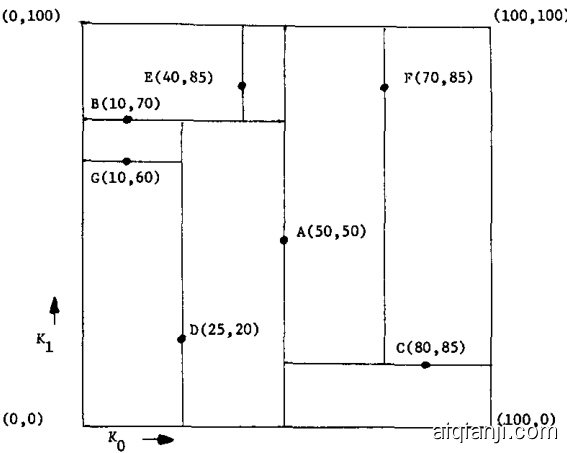
Fig. 1. Records in 2-space stored as nodes in a 2-d tree. Records in 2-space stored as nodes in a 2-d tree (boxes represent range of subtree):

图 1: 二维空间中的记录以二维树节点形式存储 (方框表示子树范围)

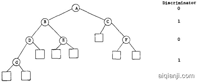
Planar graph representation of the same 2-d tree (LOSON's are expressed by left branches, HISON's by right branches, and null sons by boxes):

同一二维树的平面图表示（LOSON用左侧分支表示，HISON用右侧分支表示，空子节点用方框表示）：

Let us define node $Q$ to be $j$ -greater than node $P$ if and only if $S U C C E S S O R(P,~Q)$ is HISON, and to be $j$ -less than node $R$ if and only if $S U C C E S S O R(R,Q)$ is LOSON. It is obvious how these definitions can be used to define the $j$ -maximum and $j$ -minimum elements of a collection of nodes. The $j$ distance between nodes $P$ and $Q$ is $\mid K_{j}(P)-K_{j}(Q)\mid_{;}$ and the $j$ -nearest node of a set $s$ to node $P$ is the node $Q$ in $s$ with minimum $j$ -distance between $P$ and $Q$ . If a multiplicity of the nodes have minimum $j\mathrm{\cdot}$ distance from $\mathcal{P}$ ，then the $j\cdot$ nearest node is defined as the $j$ -minimum element in the subset of closest nodes which are $j\cdot$ greater than $P$ (or similarly, the $j\mathrm{\cdot}$ -maximum element of the nodes which are $j$ -less than $P$

我们将节点 $Q$ 定义为 $j$-大于节点 $P$ ，当且仅当 $SUCCESSOR(P,~Q)$ 为 HISON；同时将节点 $Q$ 定义为 $j$-小于节点 $R$ ，当且仅当 $SUCCESSOR(R,Q)$ 为 LOSON。显然，这些定义可用于确定节点集合中的 $j$-最大元素和 $j$-最小元素。节点 $P$ 与 $Q$ 之间的 $j$ 距离为 $\mid K_{j}(P)-K_{j}(Q)\mid_{;}$ ，而集合 $s$ 中与节点 $P$ 的 $j$-最近邻节点是 $s$ 中与 $P$ 的 $j$ 距离最小的节点 $Q$ 。若存在多个节点与 $\mathcal{P}$ 的 $j\mathrm{\cdot}$ 距离相同，则 $j\cdot$ 最近邻节点定义为这些最近邻节点中 $j\cdot$ 大于 $P$ 的子集的 $j$-最小元素 (或类似地，定义为 $j$-小于 $P$ 的节点子集中的 $j\mathrm{\cdot}$-最大元素 ) 。

We will typically use $n$ to be the number of records in the file which is stored as a $k$ -d tree, and therefore the number of nodes in the tree. We have already used $k$ as the dimensionality of the records.

我们通常用$n$表示存储在$k$ -d树中的文件记录数，即树的节点数。而$k$已用于表示记录的维度。

The keys of all nodes in the subtree of any node, say $P$ ,in a $k$ -d tree are known by $P\mathfrak{s}$ position in the tree to be bounded by certain values. For instance, if $P$ is in the HISON subtree of $Q$ , and $D I S C(Q)$ is $j_{:}$ then all nodes in $P$ are $j\mathrm{\cdot}$ greater than $Q$ ; so for any $R$ in $H I S O N(P)$ ， $K_{j}(R)\ge K_{j}(P)$ . To employ this knowledge in our algorithms, we will define a bounds array to hold the information. If $B$ is a bounds array associated with node $P$ , then $B$ has $2k$ entries, B(O), ... , $B(2k-1)$ . If $Q$ is a

在任何节点的子树中，比如 $k$ 维树中的节点 $P$，其所有节点的键值都已知由 $P$ 在树中的位置决定，并受特定值约束。例如，若 $P$ 位于 $Q$ 的 HISON 子树中，且 $DISC(Q)$ 为 $j_{:}$，则 $P$ 中所有节点的 $j$ 维键值均大于 $Q$；因此对于 $HISON(P)$ 中的任意节点 $R$，有 $K_{j}(R)\ge K_{j}(P)$。为了在算法中应用这一特性，我们将定义一个边界数组来存储这些信息。若节点 $P$ 关联的边界数组为 $B$，则 $B$ 包含 $2k$ 个条目：$B(0), ..., B(2k-1)$。假设 $Q$ 是...

descendant of $P$ , then it is true for all integers $j\in$ $[0,k-1]$ that $B(2j)\le K_{j}(Q)\le B(2j+1)$ .Bounds array $B$ is considered to be initialized if for all integers $j\in[0,k{-}1],B(2j)={-}\infty$ and $B(2j+1)=\infty$ . For example, the bounds array representing node $C$ in Figure 1 is (50, 100, 0, 100). This indicates that all $k_{0}$ values in the subtree are bounded by 50 and 100, and all $k_{1}$ values are bounded by 0 and 100.

$P$ 的子孙节点，则对于所有整数 $j\in[0,k-1]$，都有 $B(2j)\le K_{j}(Q)\le B(2j+1)$。若边界数组 $B$ 满足对所有整数 $j\in[0,k{-}1]$ 有 $B(2j)={-}\infty$ 且 $B(2j+1)=\infty$，则称该数组已完成初始化。例如，图 1 中节点 $C$ 对应的边界数组为 (50, 100, 0, 100)，表示该子树中所有 $k_{0}$ 值被约束在 50 至 100 之间，所有 $k_{1}$ 值被约束在 0 至 100 之间。

It was noted that it is not necessary to store the disc rim in at or as a field in each node, and one can see that it is easy to keep track of what kind of disc rim in at or one is visiting as one descends in a $k$ -d tree. With the idea in mind that it is superfluous to do so, we will store the disc rim in at or in each node to make the algorithms we write more easily understandable.

注意到无需将 disc rim in at 或作为字段存储在每个节点中，且可以发现在 $k$ -d 树下降过程中很容易追踪当前访问的是哪种 disc rim in at 或。虽然意识到这样做是多余的，但我们仍会在每个节点中存储 disc rim in at 以使编写的算法更易于理解。

3. Insertion

3. 插入

In this section we will first describe an algorithm that inserts a node into a $k$ -d tree We will then analyze $k$ -d trees and show that if the algorithm is used to insert random nodes into an initially empty tree the resulting tree will have the nice properties of a randomly built one-dimensional binary search tree.

在本节中，我们将首先描述一种将节点插入 $k$ -d 树的算法。随后分析 $k$ -d 树的结构特性，并证明：若使用该算法向初始为空的树中随机插入节点，最终生成的树将具备与随机构建的一维二叉搜索树相同的优良性质。

3.1 An Insertion Algorithm

3.1 一种插入算法

The algorithm used to insert a node into a $k{\cdot}\mathrm{d}$ tree is also used to search for a specific record in a tree. It is passed by a node, say $P$ If $P$ is in the tree, the algorithm returns a pointer to $P$ , and if $P$ is not in the tree it returns $\Lambda$ and inserts $P$ into the tree. Algorithm INSERT describes one way of performing such an operation.

用于将节点插入 $k{\cdot}\mathrm{d}$ 树的算法同样适用于在树中搜索特定记录。该算法接收一个节点 $P$ 作为参数：若 $P$ 存在于树中，则返回指向 $P$ 的指针；若 $P$ 不存在，则返回 $\Lambda$ 并将 $P$ 插入树中。算法 INSERT 描述了实现该操作的一种方式。

Algorithm INSERT( $k$ -d tree search and insertion)

算法 INSERT( $k$ -d树搜索与插入)

This algorithm is passed a node $P_{:}$ which is not in the tree (its HISON, LOsON, and DISC felds are not set). If there is a node in the tree with equal keys, the address of that node is returned; otherwise the node is inserted into the tree and A is returned.

该算法接收一个不在树中的节点 $P_{:}$ (其 HISON、LOsON 和 DISC 字段均未设置)。若树中存在键值相同的节点，则返回该节点地址；否则将该节点插入树中并返回 A。

3.2 Analysis of Randomly Built $k$ -d Trees

3.2 随机构建$k$ -d树分析

Consider a given binary tree of n nodes; our goal in this analysis of $k$ d trees is to show that the probability of constructing that tree by inserting $_n$ random nodes into an initially empty $k$ -d tree is the same as the probability of attaining that tree by random insertion into a one-dimensional binary search tree. Once we have shown this to be true, the theorems which have been proved about one-dimensional binary search trees will be applicable to $k{\cdot}\mathrm{d}$ trees.

考虑一个给定的包含n个节点的二叉树；我们在本次$k$d树分析中的目标是证明：通过将$_n$个随机节点插入初始为空的$k$d树来构建该树的概率，与通过随机插入一维二叉搜索树获得该树的概率相同。一旦证明此结论成立，已证关于一维二叉搜索树的定理将适用于$k{\cdot}\mathrm{d}$树。

We must first define what we mean by random nodes. Since only the relative magnitudes of the keys and the order in which the records arrive are relevant for purposes of insertion, we can assume that the records to be inserted will be defined by a $k$ -tuple of permutations of integers $1,\ldots,n$ . Then the first record to be inserted, say $P$ , would be defined by $K_{0}(P)$ , the first element in the first permutation, and so on, to $k_{k-1}(P)$ , the first element in the kth permutation. The nodes will be considered random if all of the $\left(n!\right)^{k}k$ -tuples of permutations are equally likely to occur.

我们必须首先定义随机节点的含义。由于插入操作仅与键的相对大小和记录到达的顺序相关，我们可以假设待插入的记录由一个由整数 $1,\ldots,n$ 的排列组成的 $k$ 元组定义。那么第一个要插入的记录（例如 $P$）将由第一个排列的第一个元素 $K_{0}(P)$ 定义，依此类推，直到第 $k$ 个排列的第一个元素 $k_{k-1}(P)$。如果所有 $\left(n!\right)^{k}k$ 元组的排列出现的概率均等，则认为这些节点是随机的。

Let us give each of the $n$ nodes in the binary tree t a unique identification number which is an integer between 1 and $n$ . Define $S_{i}$ as the number of nodes in the subtree of $t$ whose root is node i. To simplify our discussion of null sons let us define the identification number of a null node to be $n+1$ ; thus $S_{n+1}=0$ We will use $L_{i}$ as the number of nodes in the left subtree (or LOsON) of node $i,$ and $H_{i}$ as the number of nodes in the right subtree (or HISON); note $S_{i}=L_{i}+R_{i}+1.$

让我们为二叉树t中的每个节点分配一个唯一的标识号，该标识号为1到n之间的整数。定义$S_{i}$为以节点i为根的子树中的节点数。为了简化对空子节点的讨论，我们将空节点的标识号定义为$n+1$；因此$S_{n+1}=0$。我们将使用$L_{i}$表示节点i的左子树(或左子节点)中的节点数，$H_{i}$表示右子树(或右子节点)中的节点数；注意$S_{i}=L_{i}+R_{i}+1$。

It is important to observe the following fact about the ordering in a collection of random nodes that are to be made into a $k$ -d tree. The first node in the collection, say $P$ (which is the first to be inserted in the tree), will become the root. This induces a partition of the remaining nodes into two sub collections: those nodes that will be in $P^{\bullet}\mathbf{s}$ left (LOSON) subtree, and those that will be in the right (HISON) subtree. If $Q$ falls in the right subtree of $P$ and $R$ falls in $P^{\bullet}\mathfrak{s}$ left subtree, then their relevant ordering (that is, whether or not $Q$ precedes $R^{\prime}$ in the original collection is unimportant. The same tree would be built if P was the first element in the collection, and then came all the nodes that fell in ${\pmb P}{\pmb S}.$ right subtree, followed by all the nodes that fell in $\mathbf{\nabla}_{P}\mathbf{\cdot}\mathbf{s}$ left subtree, as long as the orderings in the left and right subcollections were maintained. A second important fact we will use is that when a collection of random nodes is split into two sub collections by this process, the resulting sub collections are themselves random collections of nodes. This is due to the original independence of keys in a given record; the partitioning in no way disturbs the independence.

关于要构建为$k$-d树的随机节点集合中的顺序，需要观察以下重要事实。集合中的第一个节点（例如$P$，即第一个插入树的节点）将成为根节点。这将剩余节点划分为两个子集：位于$P^{\bullet}\mathbf{s}$左子树（LOSON）的节点，以及位于右子树（HISON）的节点。若$Q$位于$P$的右子树而$R$位于$P^{\bullet}\mathfrak{s}$左子树，则它们在原集合中的相对顺序（即$Q$是否先于$R^{\prime}$）并不重要。只要左右子集中的顺序保持不变，即使先排列$P$，再排列所有属于${\pmb P}{\pmb S}$右子树的节点，最后排列属于$\mathbf{\nabla}_{P}\mathbf{\cdot}\mathbf{s}$左子树的节点，构建出的树结构依然相同。第二个重要事实是：当随机节点集合通过此过程被划分为两个子集时，生成的子集本身仍是随机节点集合。这是由于给定记录中键值原本的独立性——划分过程完全不会破坏这种独立性。

After having made these two observations, it is easy to compute the probability that tree t as described above results when $n$ random nodes are inserted into an initially empty $k$ -d tree. Assume that the root is a $j$ decider and that its identification number is $i$ then $S_{i}=n$ . The probability that the first record will partition the collection into two sub collections having respective sizes $L_{i}$ and $R_{i}$ is the probability that the jth key of the first element is the $(L_{i}+1)$ -th in the set of all jth keys. Because of the random nature of the nodes (all of the nodes are equally likely to be the first in the collection), this probability is $1/S_{i}$ . Now we have reduced the problem; we know that the probability of $t$ occurring is $1/S_{i}$ times the probability of both the sub collections

在得出这两个观察结果后，很容易计算出当 $n$ 个随机节点被插入初始为空的 $k$ 维树时，上述树 $t$ 出现的概率。假设根节点是一个 $j$ 维决策器，其标识号为 $i$，那么 $S_{i}=n$。第一条记录将集合划分为大小分别为 $L_{i}$ 和 $R_{i}$ 的两个子集的概率，等于第一个元素的第 $j$ 个键在所有第 $j$ 个键集合中排第 $(L_{i}+1)$ 位的概率。由于节点的随机性（所有节点成为集合中第一个元素的概率均等），该概率为 $1/S_{i}$。现在问题被简化为：树 $t$ 出现的概率等于 $1/S_{i}$ 乘以两个子集各自生成对应子树的概率之积。

forming their respective subtrees. By the second observation above, these probabilities are independent of the choice of the root of the tree and of one another. Therefore we can split the nodes into the left and right subcollections (by the first observation) and apply this analysis recursively to the left son and right son, doing so as we visit each node in the tree once and only once. It is clear that the probability of $t$ resulting is

形成各自的子树。根据上述第二个观察结果，这些概率与树的根节点选择无关且彼此独立。因此，我们可以将节点划分为左右子集合（基于第一个观察），并递归地应用于左子节点和右子节点，在遍历树的每个节点时仅执行一次该分析。显然，生成树 $t$ 的概率为

$$
P_{k}(t)=\prod_{1\leq i\leq n}1/S_{i}.
$$

We know that the standard binary search tree is a 1-d tree. Since $P_{k}(t)$ is independent of $k$ , the probability of attaining $t$ by inserting random nodes in a $k$ -d tree must be the same as that of attaining $t$ by inserting random nodes in a standard binary search tree. Indeed, the above formula for $P_{k}(t)$ was given by Knuth [5] as the probability of attaining $t$ by random insertion in a standard binary search tree. We can now apply two of the results in [5] to $k$ -d trees. Let $C_{n}$ be the number of nodes visited to find a node in a $k$ -d tree of size $n$ . Then we know that the mean of the distribution of $C_{n}$ is

我们知道标准的二叉搜索树是一种一维树。由于 $P_{k}(t)$ 与 $k$ 无关，因此在 $k$ 维树中通过随机插入节点达到 $t$ 的概率，必然与在标准二叉搜索树中通过随机插入节点达到 $t$ 的概率相同。事实上，Knuth [5] 给出的上述 $P_{k}(t)$ 公式，正是标准二叉搜索树中随机插入达到 $t$ 的概率。现在我们可以将 [5] 中的两个结果应用于 $k$ 维树。设 $C_{n}$ 为在规模为 $n$ 的 $k$ 维树中查找一个节点时访问的节点数。那么我们知道 $C_{n}$ 分布的均值是

$$
M e a n(C_{n})=2(1+1/n)H_{n}\dots3\simeq1.386\log_{2}n
$$

and the variance is

方差为

$$
V a r(C_{n})=7n^{2}-4(n+1)^{2}{H_{n}}^{(2)}-2(n+1)H_{n}+13n.
$$

Here we have used the functions

这里我们使用了函数

$$
{H_{n}}^{(x)}=\sum_{1\leq k\leq n}1/k^{x}
$$

and

以及

$$
H_{n}=H_{n}^{(1)}.
$$

Thus we know that typical insertions and record lookups in a $k$ -d tree will examine approximately $1.386\log_{2}n$ nodes.

因此我们知道，在 $k$ 维树中典型的插入和记录查找操作大约会检查 $1.386\log_{2}n$ 个节点。

4. Searching

4. 搜索

Searches are typically initiated in response to a query expressed in relation to the set of all valid records. The purpose of a search is to find in the data structure the records specified by the query. It is therefore reasonable to classify searches by the types of queries which invoke them. We will follow in the spirit of Rivest [7] as we make the primary distinction between intersection queries and best-match queries in our investigation of searching in $k$ d trees.

搜索通常始于对一组所有有效记录的查询表达。搜索的目的是在数据结构中找到查询所指定的记录。因此，根据触发搜索的查询类型对其进行分类是合理的。我们将遵循Rivest [7]的精神，在研究$k$d树中的搜索时，主要区分交集查询和最佳匹配查询。

4.1 Intersection Queries

4.1 交集查询

Intersection queries are so named because they specify that the records to be retrieved are those that intersect some subset of the set of valid records. This is by far the most common type of query. The specifications of the sets in which are all records to be retrieved can range from simply defined sets such as ${P|K_{3}(P)=7}$ to complexly defined sets like ${ P \mid (1 \leq K_1(P) \leq 5) }$ $\wedge$ $(2~\le K_{2}(P) \le 4)]$ V $(K_{7}(P)=8);$ . We will examine search strategies for three increasingly complex query types, each embodying its predecessors as special cases. The region search, the third type we will examine, is capable of searching for all records specifiable by any intersection query.

交集查询之所以如此命名，是因为它们指定要检索的记录是与有效记录集的某个子集相交的记录。这是目前最常见的查询类型。要检索的记录集的定义范围可以很简单，如 ${P|K_{3}(P)=7}$，也可以很复杂，如 ${ P \mid (1 \leq K_1(P) \leq 5) }$ $\wedge$ $(2~\le K_{2}(P) \le 4)]$ V $(K_{7}(P)=8);$ 。我们将研究三种复杂度递增的查询类型的搜索策略，每种类型都将其前身作为特例包含在内。区域搜索是我们将要研究的第三种类型，它能够搜索任何交集查询可指定的所有记录。

4.1.1 Exact Match Queries

4.1.1 精确匹配查询

The simplest type of query is the exact match query (called a “simple query" by Knuth [5], and a “point search' by Finkel and Bentley [3]), which asks if a specific record is in the data structure. The search algorithm to determine this (Algorithm INSERT) and its analysis are presented in Section 3. The only thing that remains to be said regarding the topic of exact match searching is this: If the exact match query is the only type of query to be posed, $k$ -d trees should not be used as the data structure to store the records. Though to the user the keys appear to be independent, they should be merged together into one superkey and a more well known data structure for uni dimensional storage and retrieval should be employed.

最简单的查询类型是精确匹配查询（Knuth [5] 称之为"简单查询"，Finkel 和 Bentley [3] 称之为"点搜索"），它询问数据结构中是否存在特定记录。判断该结果的搜索算法（算法 INSERT）及其分析将在第 3 节中介绍。关于精确匹配搜索主题唯一需要补充的是：如果精确匹配查询是唯一要提出的查询类型，就不应使用 $k$ -d 树作为存储记录的数据结构。尽管对用户来说键看起来是独立的，但它们应该合并成一个超级键，并采用更知名的单维存储和检索数据结构。

4.1.2 Partial Match Queries

4.1.2 部分匹配查询

The next more complex type of intersection query is one in which values are specified for a proper subset of the keys. If values are specified for $t$ keys, $t<k$ , then the query is called a “partial match query with $t$ keys specified."' Assume that $K_{s2}, \dots, K_{8t}$ ,and the values they must have to be a valid response to the query are $v_{s_{1}},v_{s_{2}},\ldots,v_{s_{t}}$ . The set of points for which we are searching is then ${P\mid K_{\mathfrak{s}_ {i}}(P) = \mathfrak{v}_ {\mathfrak{s}_{i}} for 1\leq i\leq t}$

下一种更复杂的交集查询类型是指定键值集合真子集的查询。若指定 $t$ 个键值（$t<k$），则称为"指定 $t$ 个键的部分匹配查询"。假设 ${s_{i}}$ 和 ${v_{i}}$ 是满足条件的集合，其中指定键为 $K_{s_{1}}$、$K_{s2}, \dots, K_{8t}$，其对应查询响应有效值分别为 $v_{s_{1}},v_{s_{2}},\ldots,v_{s_{t}}$。此时待搜索点集为 $[
{ P \mid K_{\mathfrak{s}_ i}(P) = \mathfrak{v}_{\mathfrak{s}_i} \text{，其中 } 1 \leq i \leq t }
]$）。

Rivest has studied this problem quite thoroughly for the case of binarily valued keys. He proposed that binary search tries be used to store the data. His ‘standard compact" tries are roughly identical to “bit-key" k-d trees. The reader interested in the binary case is referred to Rivest's thesis [7]; it contains a description of the behavior of tries (and, equivalently, $k{\cdot}\dot{\mathbf{d}}$ trees) for this application. The results presented here parallel those in that work.

Rivest针对二元值键的情况对此问题进行了深入研究。他提出使用二叉搜索字典树(trie)存储数据，其"标准紧凑型"字典树与"比特键"k-d树基本等同。对二元情形感兴趣的读者可参阅Rivest的论文[7]，其中描述了该应用场景下字典树(等价于$k{\cdot}\dot{\mathbf{d}}$树)的行为特性。本文呈现的结果与该研究具有对应关系。

A recursive search algorithm to find all nodes satisfying a partial match query for continuously valued keys is easy to define (it is shown in Section 4.1.3 that the REGION SEARCH algorithm presented here is capable of efficiently performing a partial match search, so we will merely sketch an algorithm here.) On each level of recursion the algorithm is passed a node, say $P$ If $P$ satisfies the query it is reported. Let us suppose that $P$ is a $J$ -disc rim in at or; there are now two cases we must handle. If $J=s_{i}$ for some $i_{:}$ then we need only continue our search down one subtree of $P:$ if ${\mathfrak{v}}_ {\mathfrak{s}_ {i}}<K_{J}(P)$ we go down $L O S O N(P)$ ，if $\begin{array}{r l r}{\mathfrak{p}_ {s_{i}}}&{{}>}&{K_{J}(P)}\end{array}$ we godown $H I S O N(P)$ , and if the values are equal we go down one of the subtrees depending on the definition of successor. If $J\notin{s_{i}}$ then we must continue the search down both

递归搜索算法可以很容易地定义用于查找满足连续值键部分匹配查询的所有节点（在第4.1.3节中展示了本文提出的REGION SEARCH算法能够高效执行部分匹配搜索，因此这里仅简要描述算法）。在递归的每一层，算法会接收一个节点，比如$P$。如果$P$满足查询条件，则报告该节点。假设$P$是一个$J$-判别器；现在需要处理两种情况。如果$J=s_i$对于某个$i$，那么我们只需要继续搜索$P$的一个子树：如果${\mathfrak{v}}_ {\mathfrak{s}_ {i}}<K_J(P)$，则沿$LOSON(P)$向下搜索；如果$\begin{array}{r l r}{\mathfrak{p}_{s_i}}&{{}>}&{K_J(P)}\end{array}$，则沿$HISON(P)$向下搜索；如果值相等，则根据后继定义选择其中一个子树继续搜索。如果$J\notin{s_i}$，则必须继续向下搜索两个子树。

of P's subtrees. (Implicit in the algorithm is the fact that the search continues down a subtree only if that subtree is non-null, i.e. P's SON field is not $\pmb{\Lambda}$ 一

P的子树。(算法中隐含的事实是，只有当子树非空时才会继续向下搜索，即P的SON字段不是$\pmb{\Lambda}$)

Let us now analyze the number of nodes visited by the algorithm in doing a partial match search with $t$ keys specified in an “ideal' $k$ -d tree of $^n$ nodes; a tree in which $n=2^{k h}-1$ and all leaves appear on level $k h$ (It is shown in Section 6 that such a tree is attainable for any collection of $2^{k h}-1$ nodes by using algorithm OPTIMIZE.) The search algorithm starts by visiting one node, the root, and the number of nodes visited on the next level grows by a factor of 1 (if $\boldsymbol{J}=s_{i}$ , we go down only one subtree of each node, hence visiting the same number on the next level) or two (if $J\notin{s_{i}}$ ,we have to visit both subtrees of the node, thereby visiting twice as many nodes on the next level). Since the growth rate at anylevel is a function of the disc rim in at or of that level, and the disc rim in at or s are cyclic with cycle $k$ ,the growth rate will be cyclic as well. The pessimal arrangement of keys is to have these unspecified as the first $k-t$ keys in the cycle, postponing any pruning until after a small geometric explosion. The maximum number of nodes visited during the whole search will therefore be the sum of the following series:

现在我们来分析算法在进行部分匹配搜索时访问的节点数，该搜索在一个由$n$个节点构成的“理想”$k$-d树中指定了$t$个键值（在6节中展示了通过使用算法OPTIMIZE，任何$2^{kh}-1$个节点的集合都可以构造出这样的树）。搜索算法从访问一个节点（根节点）开始，下一层访问的节点数会根据情况以1倍（如果$\boldsymbol{J}=s_{i}$，则只沿每个节点的一个子树向下，因此下一层访问的节点数不变）或2倍（如果$J\notin{s_{i}}$，则需要访问节点的两个子树，从而使下一层访问的节点数翻倍）增长。由于任何一层的增长率取决于该层的判别器，而判别器以$k$为周期循环，因此增长率也将呈现周期性变化。最不利的键值排列是将未指定的键作为周期中的前$k-t$个键，从而将剪枝推迟到经历一次小的几何级数增长之后。因此，整个搜索过程中访问的最大节点数将是以下级数的和：

$$
[
\begin{aligned}
&\frac{(k-t) \text{ elements}}{1 + 2 + \cdots + 2^{k-t-1}} + \frac{t \text{ elements}}{2^{k-t-1}} \
&\quad + t + 2^{k-t} + \cdots + 2^{(k-t)-1} \
&\quad + 2^{(k-t)(k-t)} + \cdots + 2^{k(k-t)-1}
\end{aligned}
]
$$

We can now sum this series to calculate $V(n,t)$ ,the maximum number of nodes visited during a partial match search with $t$ keys specified in an ideal tree of $n$ nodes. (For brevity, we will here define $m=k-t.$

我们现在可以对这个级数求和来计算$V(n,t)$，即在具有$n$个节点的理想树中，指定$t$个键进行部分匹配搜索时访问的最大节点数。(为简洁起见，这里定义$m=k-t$。)

$$
\begin{array}{r l}{V(n,t)=}&{\underset{0\leq i\leq k-1}{\overset{\sum}{\sum}}2^{n+1}\big[\big(\underset{0\leq j\leq m-1}{\overset{\sum}{\sum}}2^{j}\big)+2^{m-1}t\big]}\ &{=\underset{0\leq i\leq k-1}{\overset{\sum}{\sum}}2^{m+1}[2^{m}-1+2^{m-1}t]}\ &{=[(t+2)2^{m-1}-1]\underset{0\leq i\leq k-1}{\overset{\sum}{\sum}}2^{m i}}\ &{=[(t+2)2^{m-1}-1]\frac{2^{m}}{2^{m}-1}-1}\ &{=\big[(t+2)2^{m-1}-1\big]\frac{2^{m}}{2^{m}-1}-1}\ &{=\frac{[(t+2)2^{m-1}-1]}{2^{m}-1}(2^{m k}-1).}\end{array}
$$

Since we know 2mh = 2(m/k)kh $2^{m h}=2^{(m/k)k h}=(2^{k h})^{m/k}=(n+1)^{m/k},$ wesee

既然我们知道 $2^{m h}=2^{(m/k)k h}=(2^{k h})^{m/k}=(n+1)^{m/k},$ 那么可得

$$
V(n,t)=\frac{[(t+2)2^{m-1}-1]}{2^{m}-1}[(n+1)^{m/k}-1].
$$

The amount of work done in any partial match search with $t$ keys specified in an ideal tree of $n$ nodes is therefore $c n^{m/k}+d$ for some small constants $c$ and $d$ This has been conjectured by Rivest [7] to be a lower bound for the average amount of work done in a partial match search; by construction we have shown this to be an upper bound not only for the average but for all partial match queries.

在具有 $n$ 个节点的理想树中，指定 $t$ 个键进行任何部分匹配搜索时，所做的工作量为 $c n^{m/k}+d$，其中 $c$ 和 $d$ 为较小的常数。Rivest [7] 推测这是部分匹配搜索平均工作量的下界；通过构造，我们证明了这不仅是平均值，也是所有部分匹配查询的上界。

All of our analysis has been for the case of the perfectly balanced tree; the one in which we might expect to have the fastest searches. However, Rivest [7] has shown that the perfectly balanced trees have the highest average retrieval time. Therefore the results that we have shown are an expected upper bound on the retrieval time required by the algorithm.

我们所有的分析都针对完全平衡树(perfectly balanced tree)的情况，这种树型理论上应具有最快的搜索速度。然而Rivest [7]已证明完全平衡树具有最高的平均检索时间。因此我们展示的结果是该算法所需检索时间的预期上限。

4.1.3 Region Queries

4.1.3 区域查询

The most general type of intersection query is one in which any region at all may be specified as the set with which the records to be retrieved must intersect, hence its name “region query."' This query is the same as the “region search' query described by Finkel and Bentley [3] and facilitates the range, best match with restricted distance, and boolean queries described by Knuth [5] and Rivest [7]. Any subset of the set of valid records region can be specified in a region query, so it is therefore the most general intersection query possible. (An exact match query corresponds to the region being a point, a partial match query with $t$ keys specified corresponds to the region being a $k\mathrm{ - }t$ dimensional hyperplane.)

最通用的交集查询类型是允许指定任意区域作为检索记录必须相交的集合，因此得名“区域查询”。这种查询与Finkel和Bentley [3] 描述的“区域搜索”查询相同，并支持Knuth [5] 和Rivest [7] 提出的范围查询、受限距离最佳匹配查询以及布尔查询。在区域查询中可以指定有效记录区域的任何子集，因此这是可能的最通用交集查询。(精确匹配查询对应区域为点的情况，指定$t$个键的部分匹配查询对应$k\mathrm{ - }t$维超平面区域。)

The algorithm to accomplish a region search need not specifically know the definition of the region in which it is searching; rather it finds out all it needs to know by calling two functions which describe the region. The first, IN_REGION, is passed a node in the tree and returns true if and only if that node is contained in the region. The function BOUNDS INTERSECT REGION is passed a bounds array and returns true if and only if the region intersects the hyper-rectangle described by the bounds array. Nor does the algorithm know what to do once it finds a node in the region; it calls procedure FOUND to report all nodes it finds in the region. A recursive definition of the general intersection query search algorithm is given below. It would be invoked initially by the command REGION $S E A R C H(R O O T,B)$ where $B$ is a bounds array ini- tialized as described in Section 2. [See next page.]

完成区域搜索的算法无需具体知晓搜索区域的定义，而是通过调用两个描述区域的函数获取所需信息。第一个函数IN_REGION接收树中的一个节点，当且仅当该节点位于区域内时返回true。第二个函数BOUNDS_INTERSECT_REGION接收边界数组，当且仅当区域与边界数组描述的超矩形相交时返回true。该算法在发现区域内的节点时也不直接处理，而是调用FOUND过程来报告所有在区域内找到的节点。通用交集查询搜索算法的递归定义如下所示，初始调用命令为REGION_SEARCH(ROOT,B)，其中B是如第2节所述初始化的边界数组。[见下页]

Algorithm REGION SEARCH uses the bounds stored at each node of the tree to determine whether it is possible that any descendants of the node might lie in the region being searched. A subtree is visited by the algorithm if and only if this possibility exists. Consequently, the algorithm visits as few nodes as possible, given the limited information stored at each node. In this sense, REGION SEARCH is an optimal algorithm for region searches in $k$ -d trees as we have described them.

算法 REGION SEARCH 利用存储在树各节点上的边界信息，判断该节点的后代是否可能位于搜索区域内。当且仅当存在这种可能性时，算法才会访问该子树。因此，在节点存储信息有限的条件下，该算法实现了最小化的节点访问量。从这个意义上说，对于我们所描述的 $k$ 维树结构而言，REGION SEARCH 是区域搜索的最优算法。

The versatility of algorithm REGION SEARCH makes its formal analysis extremely difficult. Its per

算法REGION SEARCH的多样性使其形式化分析极为困难。

(cont'd in col. 2, next

[论文翻译]用于关联搜索的多维二叉搜索树

原文地址：https://dl.acm.org/doi/pdf/10.1145/361002.361007