ALBERT: A LITE BERT FOR SELF-SUPERVISED LEARNING OF LANGUAGE REPRESENTATIONS
ALBERT: 一种轻量级BERT模型用于语言表征的自监督学习
ABSTRACT
摘要
Increasing model size when pre training natural language representations often results in improved performance on downstream tasks. However, at some point further model increases become harder due to GPU/TPU memory limitations and longer training times. To address these problems, we present two parameterreduction techniques to lower memory consumption and increase the training speed of BERT (Devlin et al., 2019). Comprehensive empirical evidence shows that our proposed methods lead to models that scale much better compared to the original BERT. We also use a self-supervised loss that focuses on modeling inter-sentence coherence, and show it consistently helps downstream tasks with multi-sentence inputs. As a result, our best model establishes new state-of-the-art results on the GLUE, RACE, and SQuAD benchmarks while having fewer parameters compared to BERT-large. The code and the pretrained models are available at https://github.com/google-research/ALBERT.
在预训练自然语言表示时增加模型规模通常能提升下游任务的表现。但随着模型持续增大,GPU/TPU内存限制和训练时间延长会导致进一步扩展变得困难。为解决这些问题,我们提出两种参数压缩技术来降低内存占用并加速BERT训练(Devlin et al., 2019)。大量实验证明,相比原始BERT,我们提出的方法能使模型获得更优的扩展性。我们还采用了一种专注于建模句子间连贯性的自监督损失函数,实验表明该设计能持续提升多句子输入的下游任务表现。最终,我们的最佳模型在参数量少于BERT-large的情况下,于GLUE、RACE和SQuAD基准测试中创造了新的性能记录。代码与预训练模型已开源:https://github.com/google-research/ALBERT。
1 INTRODUCTION
1 引言
Full network pre-training (Dai & Le, 2015; Radford et al., 2018; Devlin et al., 2019; Howard & Ruder, 2018) has led to a series of breakthroughs in language representation learning. Many nontrivial NLP tasks, including those that have limited training data, have greatly benefited from these pre-trained models. One of the most compelling signs of these breakthroughs is the evolution of machine performance on a reading comprehension task designed for middle and high-school English exams in China, the RACE test (Lai et al., 2017): the paper that originally describes the task and formulates the modeling challenge reports then state-of-the-art machine accuracy at $44.1%$ ; the latest published result reports their model performance at $83.2%$ (Liu et al., 2019); the work we present here pushes it even higher to $89.4%$ , a stunning $45.3%$ improvement that is mainly attributable to our current ability to build high-performance pretrained language representations.
全网络预训练 (Dai & Le, 2015; Radford et al., 2018; Devlin et al., 2019; Howard & Ruder, 2018) 在语言表征学习领域引发了一系列突破。许多重要的自然语言处理任务 (包括训练数据有限的任务) 都从这些预训练模型中受益匪浅。这些突破最显著的标志之一是中国初高中英语考试阅读理解任务 RACE (Lai et al., 2017) 上机器表现的演进: 最初描述该任务并提出建模挑战的论文报告的最先进机器准确率为 $44.1%$ ; 最新发表的结果显示其模型性能达到 $83.2%$ (Liu et al., 2019) ; 本文工作将其进一步提升至 $89.4%$ , 这惊人的 $45.3%$ 提升主要归功于当前构建高性能预训练语言表征的能力。
Evidence from these improvements reveals that a large network is of crucial importance for achieving state-of-the-art performance (Devlin et al., 2019; Radford et al., 2019). It has become common practice to pre-train large models and distill them down to smaller ones (Sun et al., 2019; Turc et al., 2019) for real applications. Given the importance of model size, we ask: Is having better NLP models as easy as having larger models?
这些改进的证据表明,大型网络对于实现最先进性能至关重要 (Devlin et al., 2019; Radford et al., 2019)。预训练大模型并将其蒸馏为更小模型 (Sun et al., 2019; Turc et al., 2019) 已成为实际应用中的常见做法。鉴于模型规模的重要性,我们不禁要问:获得更好的自然语言处理 (NLP) 模型是否只需构建更大的模型?
An obstacle to answering this question is the memory limitations of available hardware. Given that current state-of-the-art models often have hundreds of millions or even billions of parameters, it is easy to hit these limitations as we try to scale our models. Training speed can also be significantly hampered in distributed training, as the communication overhead is directly proportional to the number of parameters in the model.
回答这个问题的一个障碍是现有硬件的内存限制。鉴于当前最先进的模型通常具有数亿甚至数十亿参数,在尝试扩展模型时很容易触及这些限制。分布式训练中的训练速度也会受到显著阻碍,因为通信开销与模型参数数量成正比。
Existing solutions to the aforementioned problems include model parallel iz ation (Shazeer et al., 2018; Shoeybi et al., 2019) and clever memory management (Chen et al., 2016; Gomez et al., 2017).
现有解决方案包括模型并行化 (Shazeer et al., 2018; Shoeybi et al., 2019) 和智能内存管理 (Chen et al., 2016; Gomez et al., 2017)。
These solutions address the memory limitation problem, but not the communication overhead. In this paper, we address all of the aforementioned problems, by designing A Lite BERT (ALBERT) architecture that has significantly fewer parameters than a traditional BERT architecture.
这些解决方案解决了内存限制问题,但并未降低通信开销。本文通过设计参数量远少于传统BERT架构的轻量级BERT (ALBERT) 架构,解决了上述所有问题。
ALBERT incorporates two parameter reduction techniques that lift the major obstacles in scaling pre-trained models. The first one is a factorized embedding parameter iz ation. By decomposing the large vocabulary embedding matrix into two small matrices, we separate the size of the hidden layers from the size of vocabulary embedding. This separation makes it easier to grow the hidden size without significantly increasing the parameter size of the vocabulary embeddings. The second technique is cross-layer parameter sharing. This technique prevents the parameter from growing with the depth of the network. Both techniques significantly reduce the number of parameters for BERT without seriously hurting performance, thus improving parameter-efficiency. An ALBERT configuration similar to BERT-large has 18x fewer parameters and can be trained about $1.7\mathbf{X}$ faster. The parameter reduction techniques also act as a form of regular iz ation that stabilizes the training and helps with generalization.
ALBERT采用了两项参数削减技术,有效解决了预训练模型规模化过程中的主要障碍。第一项是因子化嵌入参数化 (factorized embedding parameterization) ,通过将大型词表嵌入矩阵分解为两个小矩阵,实现了隐藏层维度与词表嵌入维度的解耦。这种分离使得增加隐藏层维度时,不会显著增加词表嵌入的参数规模。第二项技术是跨层参数共享,该技术能防止参数量随网络深度增长。这两种技术在基本不影响BERT性能的前提下大幅减少了参数量,从而提升了参数效率。与BERT-large配置相似的ALBERT模型参数量减少了18倍,训练速度提升约$1.7\mathbf{X}$。这些参数削减技术还起到了正则化作用,稳定了训练过程并提升了泛化能力。
To further improve the performance of ALBERT, we also introduce a self-supervised loss for sentence-order prediction (SOP). SOP primary focuses on inter-sentence coherence and is designed to address the ineffectiveness (Yang et al., 2019; Liu et al., 2019) of the next sentence prediction (NSP) loss proposed in the original BERT.
为进一步提升ALBERT的性能,我们还引入了句子顺序预测(SOP)的自监督损失。SOP主要关注句间连贯性,旨在解决原始BERT中提出的下一句预测(NSP)损失效率低下的问题(Yang et al., 2019; Liu et al., 2019)。
As a result of these design decisions, we are able to scale up to much larger ALBERT configurations that still have fewer parameters than BERT-large but achieve significantly better performance. We establish new state-of-the-art results on the well-known GLUE, SQuAD, and RACE benchmarks for natural language understanding. Specifically, we push the RACE accuracy to $89.4%$ , the GLUE benchmark to 89.4, and the F1 score of SQuAD 2.0 to 92.2.
由于这些设计决策,我们能够扩展至更大的ALBERT配置,其参数量仍少于BERT-large但性能显著提升。我们在自然语言理解的经典基准测试GLUE、SQuAD和RACE上创造了新的最优成绩。具体而言,我们将RACE准确率提升至$89.4%$,GLUE基准得分提升至89.4,SQuAD 2.0的F1分数提升至92.2。
2 RELATED WORK
2 相关工作
2.1 SCALING UP REPRESENTATION LEARNING FOR NATURAL LANGUAGE
2.1 自然语言表征学习的规模化扩展
Learning representations of natural language has been shown to be useful for a wide range of NLP tasks and has been widely adopted (Mikolov et al., 2013; Le & Mikolov, 2014; Dai & Le, 2015; Peters et al., 2018; Devlin et al., 2019; Radford et al., 2018; 2019). One of the most significant changes in the last two years is the shift from pre-training word embeddings, whether standard (Mikolov et al., 2013; Pennington et al., 2014) or contextual i zed (McCann et al., 2017; Peters et al., 2018), to full-network pre-training followed by task-specific fine-tuning (Dai & Le, 2015; Radford et al., 2018; Devlin et al., 2019). In this line of work, it is often shown that larger model size improves performance. For example, Devlin et al. (2019) show that across three selected natural language understanding tasks, using larger hidden size, more hidden layers, and more attention heads always leads to better performance. However, they stop at a hidden size of 1024, presumably because of the model size and computation cost problems.
学习自然语言的表示已被证明对广泛的自然语言处理(NLP)任务非常有用,并得到了广泛采用 (Mikolov et al., 2013; Le & Mikolov, 2014; Dai & Le, 2015; Peters et al., 2018; Devlin et al., 2019; Radford et al., 2018; 2019)。过去两年最显著的变化是从预训练词嵌入(无论是标准的 (Mikolov et al., 2013; Pennington et al., 2014) 还是上下文敏感的 (McCann et al., 2017; Peters et al., 2018))转向全网络预训练后进行任务特定微调 (Dai & Le, 2015; Radford et al., 2018; Devlin et al., 2019)。在这类工作中,通常表明更大的模型规模能提升性能。例如,Devlin et al. (2019) 表明,在三个选定的自然语言理解任务中,使用更大的隐藏层大小、更多的隐藏层和更多的注意力头总能带来更好的性能。然而,他们将隐藏层大小停留在1024,推测是由于模型规模和计算成本问题。
It is difficult to experiment with large models due to computational constraints, especially in terms of GPU/TPU memory limitations. Given that current state-of-the-art models often have hundreds of millions or even billions of parameters, we can easily hit memory limits. To address this issue, Chen et al. (2016) propose a method called gradient check pointing to reduce the memory requirement to be sublinear at the cost of an extra forward pass. Gomez et al. (2017) propose a way to reconstruct each layer’s activation s from the next layer so that they do not need to store the intermediate activation s. Both methods reduce the memory consumption at the cost of speed. Raffel et al. (2019) proposed to use model parallel iz ation to train a giant model. In contrast, our parameter-reduction techniques reduce memory consumption and increase training speed.
由于计算资源限制,尤其是GPU/TPU内存限制,对大模型进行实验具有挑战性。鉴于当前最先进的模型通常具有数亿甚至数十亿参数,我们很容易触及内存上限。为解决这一问题,Chen等人 (2016) 提出了一种称为梯度检查点 (gradient check pointing) 的方法,通过额外一次前向传播的代价将内存需求降至亚线性级别。Gomez等人 (2017) 提出通过下一层重构每一层的激活值 (activation),从而无需存储中间激活值。这两种方法都以牺牲速度为代价降低内存消耗。Raffel等人 (2019) 提出使用模型并行化 (model parallelization) 来训练巨型模型。相比之下,我们的参数削减技术既能降低内存消耗,又能提升训练速度。
2.2 CROSS-LAYER PARAMETER SHARING
2.2 跨层参数共享
The idea of sharing parameters across layers has been previously explored with the Transformer architecture (Vaswani et al., 2017), but this prior work has focused on training for standard encoderdecoder tasks rather than the pre training/finetuning setting. Different from our observations, Dehghani et al. (2018) show that networks with cross-layer parameter sharing (Universal Transformer, UT) get better performance on language modeling and subject-verb agreement than the standard transformer. Very recently, Bai et al. (2019) propose a Deep Equilibrium Model (DQE) for transformer networks and show that DQE can reach an equilibrium point for which the input embedding and the output embedding of a certain layer stay the same. Our observations show that our embeddings are oscillating rather than converging. Hao et al. (2019) combine a parameter-sharing transformer with the standard one, which further increases the number of parameters of the standard transformer.
在Transformer架构中共享参数的想法此前已有研究 (Vaswani等人,2017) ,但这些工作主要针对标准编码器-解码器任务的训练,而非预训练/微调场景。与我们的发现不同,Dehghani等人 (2018) 证明跨层参数共享网络 (通用Transformer,UT) 在语言建模和主谓一致任务上表现优于标准Transformer。最近,Bai等人 (2019) 提出Transformer网络的深度均衡模型 (DQE) ,并证明DQE能使特定层的输入嵌入和输出嵌入达到均衡状态。而我们的实验显示嵌入向量呈现振荡而非收敛状态。Hao等人 (2019) 将参数共享Transformer与标准Transformer结合,这反而增加了标准Transformer的参数规模。
2.3 SENTENCE ORDERING OBJECTIVES
2.3 句子排序目标
ALBERT uses a pre training loss based on predicting the ordering of two consecutive segments of text. Several researchers have experimented with pre training objectives that similarly relate to discourse coherence. Coherence and cohesion in discourse have been widely studied and many phenomena have been identified that connect neighboring text segments (Hobbs, 1979; Halliday & Hasan, 1976; Grosz et al., 1995). Most objectives found effective in practice are quite simple. Skipthought (Kiros et al., 2015) and FastSent (Hill et al., 2016) sentence embeddings are learned by using an encoding of a sentence to predict words in neighboring sentences. Other objectives for sentence embedding learning include predicting future sentences rather than only neighbors (Gan et al., 2017) and predicting explicit discourse markers (Jernite et al., 2017; Nie et al., 2019). Our loss is most similar to the sentence ordering objective of Jernite et al. (2017), where sentence embeddings are learned in order to determine the ordering of two consecutive sentences. Unlike most of the above work, however, our loss is defined on textual segments rather than sentences. BERT (Devlin et al., 2019) uses a loss based on predicting whether the second segment in a pair has been swapped with a segment from another document. We compare to this loss in our experiments and find that sentence ordering is a more challenging pre training task and more useful for certain downstream tasks. Concurrently to our work, Wang et al. (2019) also try to predict the order of two consecutive segments of text, but they combine it with the original next sentence prediction in a three-way classification task rather than empirically comparing the two.
ALBERT采用基于预测连续两段文本顺序的预训练损失函数。多位研究者尝试过与语篇连贯性相关的预训练目标。语篇中的连贯与衔接已被广泛研究,学界已发现许多连接相邻文本段的现象 (Hobbs, 1979; Halliday & Hasan, 1976; Grosz et al., 1995)。实践中有效的目标大多较为简单:Skipthought (Kiros et al., 2015) 和FastSent (Hill et al., 2016) 通过使用句子编码预测相邻句子中的词来学习句子嵌入;其他句子嵌入学习目标包括预测未来句子而非仅限相邻句 (Gan et al., 2017),以及预测显式语篇标记 (Jernite et al., 2017; Nie et al., 2019)。我们的损失函数与Jernite等人 (2017) 的句子排序目标最为相似,其通过确定连续两句的顺序来学习句子嵌入。但与上述多数工作不同,我们的损失函数作用于文本段而非句子。BERT (Devlin et al., 2019) 使用基于预测文本对中第二段是否被替换为其他文档片段的损失函数。实验表明,句子排序是更具挑战性的预训练任务,对某些下游任务更有效。与我们同期的工作中,Wang等人 (2019) 也尝试预测连续文本段的顺序,但他们将其与原始下一句预测结合为三向分类任务,而未对两者进行实证比较。
3 THE ELEMENTS OF ALBERT
3 ALBERT 的构成要素
In this section, we present the design decisions for ALBERT and provide quantified comparisons against corresponding configurations of the original BERT architecture (Devlin et al., 2019).
在本节中,我们将介绍ALBERT的设计决策,并提供与原始BERT架构 (Devlin et al., 2019) 相应配置的量化对比。
3.1 MODEL ARCHITECTURE CHOICES
3.1 模型架构选择
The backbone of the ALBERT architecture is similar to BERT in that it uses a transformer encoder (Vaswani et al., 2017) with GELU nonlinear i ties (Hendrycks & Gimpel, 2016). We follow the BERT notation conventions and denote the vocabulary embedding size as $E$ , the number of encoder layers as $L$ , and the hidden size as $H$ . Following Devlin et al. (2019), we set the feed-forward/filter size to be $4H$ and the number of attention heads to be $H/64$ .
ALBERT架构的主干与BERT类似,都采用了Transformer编码器 (Vaswani et al., 2017) 和GELU非线性激活函数 (Hendrycks & Gimpel, 2016)。我们沿用BERT的符号约定:词汇嵌入维度记为$E$,编码器层数记为$L$,隐藏层维度记为$H$。参照Devlin et al. (2019)的设置,前馈网络/滤波器维度设为$4H$,注意力头数设为$H/64$。
There are three main contributions that ALBERT makes over the design choices of BERT.
ALBERT相比BERT的设计选择主要有三点贡献。
Factorized embedding parameter iz ation. In BERT, as well as subsequent modeling improvements such as XLNet (Yang et al., 2019) and RoBERTa (Liu et al., 2019), the WordPiece embedding size $E$ is tied with the hidden layer size $H$ , i.e., $E\equiv H$ . This decision appears suboptimal for both modeling and practical reasons, as follows.
因子化嵌入参数化。在BERT及后续改进模型如XLNet (Yang等人,2019) 和RoBERTa (Liu等人,2019) 中,WordPiece嵌入维度$E$与隐藏层维度$H$绑定,即$E\equiv H$。从建模和实际应用角度来看,这种设计存在以下次优问题:
From a modeling perspective, WordPiece embeddings are meant to learn context-independent representations, whereas hidden-layer embeddings are meant to learn context-dependent representations. As experiments with context length indicate (Liu et al., 2019), the power of BERT-like representations comes from the use of context to provide the signal for learning such context-dependent representations. As such, untying the WordPiece embedding size $E$ from the hidden layer size $H$ allows us to make a more efficient usage of the total model parameters as informed by modeling needs, which dictate that $H\gg E$ .
从建模角度来看,WordPiece嵌入旨在学习上下文无关的表示,而隐藏层嵌入则用于学习上下文相关的表示。正如上下文长度实验所示 [20],类BERT表示的优势源于利用上下文信号来学习这种上下文相关的表示。因此,将WordPiece嵌入尺寸$E$与隐藏层尺寸$H$解耦,能让我们根据建模需求更高效地利用总参数量——该需求决定了$H\gg E$的关系。
From a practical perspective, natural language processing usually require the vocabulary size $V$ to be large.1 If $E\equiv H$ , then increasing $H$ increases the size of the embedding matrix, which has size
从实践角度来看,自然语言处理通常需要词汇表大小 $V$ 足够大。若 $E\equiv H$ ,则增大 $H$ 会导致嵌入矩阵 (embedding matrix) 的尺寸增加,其尺寸为
$V\times E$ . This can easily result in a model with billions of parameters, most of which are only updated sparsely during training.
$V\times E$。这很容易导致模型具有数十亿参数,其中大多数在训练期间仅稀疏更新。
Therefore, for ALBERT we use a factorization of the embedding parameters, decomposing them into two smaller matrices. Instead of projecting the one-hot vectors directly into the hidden space of size $H$ , we first project them into a lower dimensional embedding space of size $E$ , and then project it to the hidden space. By using this decomposition, we reduce the embedding parameters from $O(V\times H)$ to $O(\bar{V}\times E\dot{+}E\dot{\times}H)$ . This parameter reduction is significant when $H\gg E$ . We choose to use the same E for all word pieces because they are much more evenly distributed across documents compared to whole-word embedding, where having different embedding size (Grave et al. (2017); Baevski & Auli (2018); Dai et al. (2019) ) for different words is important.
因此,对于ALBERT模型,我们采用了嵌入参数因式分解策略,将其分解为两个较小的矩阵。我们不再将独热向量直接投影到维度为$H$的隐藏空间,而是先将其投影到维度为$E$的低维嵌入空间,再映射至隐藏空间。通过这种分解方式,嵌入参数量从$O(V\times H)$降至$O(\bar{V}\times E\dot{+}E\dot{\times}H)$。当$H\gg E$时,这种参数量削减效果尤为显著。我们为所有词片段(word piece)选择相同的$E$值,因为相较于需要为不同单词设置不同嵌入维度(Grave et al. (2017); Baevski & Auli (2018); Dai et al. (2019))的整词嵌入,词片段在文档中的分布更为均匀。
Cross-layer parameter sharing. For ALBERT, we propose cross-layer parameter sharing as another way to improve parameter efficiency. There are multiple ways to share parameters, e.g., only sharing feed-forward network (FFN) parameters across layers, or only sharing attention parameters. The default decision for ALBERT is to share all parameters across layers. All our experiments use this default decision unless otherwise specified. We compare this design decision against other strategies in our experiments in Sec. 4.5.
跨层参数共享。对于ALBERT,我们提出跨层参数共享作为另一种提升参数效率的方法。参数共享存在多种方式,例如仅在各层间共享前馈网络(FFN)参数,或仅共享注意力参数。ALBERT的默认方案是在所有层间共享全部参数。除非另有说明,我们所有实验均采用这一默认方案。我们将在4.5节的实验中对比该设计方案与其他策略的效果。
Similar strategies have been explored by Dehghani et al. (2018) (Universal Transformer, UT) and Bai et al. (2019) (Deep Equilibrium Models, DQE) for Transformer networks. Different from our observations, Dehghani et al. (2018) show that UT outperforms a vanilla Transformer. Bai et al. (2019) show that their DQEs reach an equilibrium point for which the input and output embedding of a certain layer stay the same. Our measurement on the L2 distances and cosine similarity show that our embeddings are oscillating rather than converging.
Dehghani等人(2018)(Universal Transformer, UT)和Bai等人(2019)(Deep Equilibrium Models, DQE)针对Transformer网络探索了类似策略。与我们的观察不同,Dehghani等人(2018)表明UT优于原始Transformer。Bai等人(2019)证明他们的DQE能达到某个平衡点,使得特定层的输入和输出嵌入保持不变。而我们对L2距离和余弦相似度的测量显示,我们的嵌入是在振荡而非收敛。
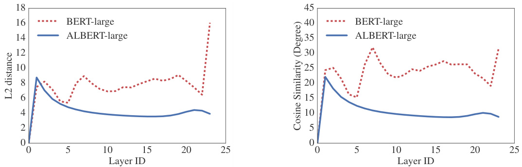
Figure 1: The L2 distances and cosine similarity (in terms of degree) of the input and output embedding of each layer for BERT-large and ALBERT-large.
图 1: BERT-large 和 ALBERT-large 各层输入与输出嵌入的 L2 距离及余弦相似度(以角度表示)。
Figure 1 shows the L2 distances and cosine similarity of the input and output embeddings for each layer, using BERT-large and ALBERT-large configurations (see Table 1). We observe that the transitions from layer to layer are much smoother for ALBERT than for BERT. These results show that weight-sharing has an effect on stabilizing network parameters. Although there is a drop for both metrics compared to BERT, they nevertheless do not converge to 0 even after 24 layers. This shows that the solution space for ALBERT parameters is very different from the one found by DQE.
图1展示了使用BERT-large和ALBERT-large配置(见表1)时,各层输入与输出嵌入向量的L2距离和余弦相似度。我们观察到ALBERT的层间变化比BERT更为平滑。这些结果表明权重共享对稳定网络参数具有影响。尽管两项指标相较BERT均有所下降,但即便经过24层处理后仍未收敛至0。这说明ALBERT参数的解空间与DQE发现的解空间存在显著差异。
Inter-sentence coherence loss. In addition to the masked language modeling (MLM) loss (Devlin et al., 2019), BERT uses an additional loss called next-sentence prediction (NSP). NSP is a binary classification loss for predicting whether two segments appear consecutively in the original text, as follows: positive examples are created by taking consecutive segments from the training corpus; negative examples are created by pairing segments from different documents; positive and negative examples are sampled with equal probability. The NSP objective was designed to improve performance on downstream tasks, such as natural language inference, that require reasoning about the relationship between sentence pairs. However, subsequent studies (Yang et al., 2019; Liu et al., 2019) found NSP’s impact unreliable and decided to eliminate it, a decision supported by an improvement in downstream task performance across several tasks.
句间连贯性损失。除了掩码语言建模(MLM)损失(Devlin等人,2019)外,BERT还使用了一种称为下一句预测(NSP)的额外损失。NSP是一个二元分类损失,用于预测两个片段是否在原始文本中连续出现,具体如下:正例通过从训练语料中提取连续片段生成;负例通过配对不同文档的片段生成;正负例以相同概率采样。NSP目标旨在提升需要推理句对关系的下游任务(如自然语言推理)性能。但后续研究(Yang等人,2019;Liu等人,2019)发现NSP的影响不可靠,决定取消该机制,这一决策得到了多项任务下游性能提升的支持。
We conjecture that the main reason behind NSP’s ineffectiveness is its lack of difficulty as a task, as compared to MLM. As formulated, NSP conflates topic prediction and coherence prediction in a
我们推测NSP(Next Sentence Prediction)无效的主要原因在于,与MLM(Masked Language Modeling)相比,其任务难度不足。按照现有设计,NSP将主题预测和连贯性预测混为一谈。
| 模型 | 版本 | 参数量 | 层数 | 隐藏层维度 | 嵌入维度 | 参数共享 |
|---|---|---|---|---|---|---|
| BERT | base | 108M | 12 | 768 | 768 | False |
| large | 334M | 24 | 1024 | 1024 | False | |
| ALBERT | base | 12M | 12 | 768 | 128 | True |
| large | 18M | 24 | 1024 | 128 | True | |
| xlarge | 60M | 24 | 2048 | 128 | True | |
| xxlarge | 235M | 12 | 4096 | 128 | True |
Table 1: The configurations of the main BERT and ALBERT models analyzed in this paper.
表 1: 本文分析的主要 BERT 和 ALBERT 模型配置。
single task2. However, topic prediction is easier to learn compared to coherence prediction, and also overlaps more with what is learned using the MLM loss.
然而,与连贯性预测相比,主题预测更容易学习,并且与使用MLM损失学习的内容重叠更多。
We maintain that inter-sentence modeling is an important aspect of language understanding, but we propose a loss based primarily on coherence. That is, for ALBERT, we use a sentence-order prediction (SOP) loss, which avoids topic prediction and instead focuses on modeling inter-sentence coherence. The SOP loss uses as positive examples the same technique as BERT (two consecutive segments from the same document), and as negative examples the same two consecutive segments but with their order swapped. This forces the model to learn finer-grained distinctions about discourse-level coherence properties. As we show in Sec. 4.6, it turns out that NSP cannot solve the SOP task at all (i.e., it ends up learning the easier topic-prediction signal, and performs at randombaseline level on the SOP task), while SOP can solve the NSP task to a reasonable degree, presumably based on analyzing misaligned coherence cues. As a result, ALBERT models consistently improve downstream task performance for multi-sentence encoding tasks.
我们坚持认为句子间建模是语言理解的重要方面,但提出了一种主要基于连贯性的损失函数。具体而言,ALBERT采用句子顺序预测(SOP)损失,避免主题预测而专注于句子间连贯性建模。该损失函数以BERT相同的技术构建正例(来自同一文档的两个连续段落),负例则保持相同段落但交换顺序。这种设计迫使模型学习语篇层面连贯性的细粒度区分特征。如第4.6节所示,NSP完全无法解决SOP任务(最终仅学习到更简单的主题预测信号,在SOP任务上表现与随机基线相当),而SOP能较好解决NSP任务,这可能是基于对错位连贯性线索的分析。因此,ALBERT模型在多句子编码任务中持续提升下游任务表现。
3.2 MODEL SETUP
3.2 模型设置
We present the differences between BERT and ALBERT models with comparable hyper parameter settings in Table 1. Due to the design choices discussed above, ALBERT models have much smaller parameter size compared to corresponding BERT models.
我们在表1中展示了具有可比超参数设置的BERT和ALBERT模型之间的差异。由于上述设计选择,ALBERT模型的参数量比对应的BERT模型小得多。
For example, ALBERT-large has about $18\mathrm{x}$ fewer parameters compared to BERT-large, 18M versus 334M. An ALBERT-xlarge configuration with $H=2048$ has only 60M parameters and an ALBERT-xxlarge configuration with $H=4096$ has 233M parameters, i.e., around $70%$ of BERTlarge’s parameters. Note that for ALBERT-xxlarge, we mainly report results on a 12-layer network because a 24-layer network (with the same configuration) obtains similar results but is computationally more expensive.
例如,ALBERT-large 的参数数量比 BERT-large 少约 $18\mathrm{x}$,分别为 18M 和 334M。配置为 $H=2048$ 的 ALBERT-xlarge 仅有 60M 参数,而 $H=4096$ 的 ALBERT-xxlarge 则有 233M 参数,约为 BERT-large 参数的 $70%$。需要注意的是,对于 ALBERT-xxlarge,我们主要报告了 12 层网络的结果,因为 24 层网络(相同配置)虽然结果相似,但计算成本更高。
This improvement in parameter efficiency is the most important advantage of ALBERT’s design choices. Before we can quantify this advantage, we need to introduce our experimental setup in more detail.
参数效率的提升是ALBERT设计决策中最重要的优势。在量化这一优势之前,我们需要更详细地介绍实验设置。
4 EXPERIMENTAL RESULTS
4 实验结果
4.1 EXPERIMENTAL SETUP
4.1 实验设置
To keep the comparison as meaningful as possible, we follow the BERT (Devlin et al., 2019) setup in using the BOOKCORPUS (Zhu et al., 2015) and English Wikipedia (Devlin et al., 2019) for pretraining baseline models. These two corpora consist of around 16GB of uncompressed text. We format our inputs as “[CLS] $x_{1}$ [SEP] $x_{2}$ [SEP]”, where $x_{1}=x_{1,1},x_{1,2}\cdot\cdot\cdot$ and $x_{2}=x_{1,1},x_{1,2}\cdot\cdot\cdot$ are two segments.3 We always limit the maximum input length to 512, and randomly generate input sequences shorter than 512 with a probability of $10%$ . Like BERT, we use a vocabulary size of 30,000, tokenized using Sentence Piece (Kudo & Richardson, 2018) as in XLNet (Yang et al., 2019).
为了使对比尽可能有意义,我们遵循BERT (Devlin et al., 2019)的设置,使用BOOKCORPUS (Zhu et al., 2015)和英文维基百科(Devlin et al., 2019)作为预训练基准模型的数据集。这两个语料库包含约16GB未压缩文本。我们将输入格式化为"[CLS] $x_{1}$ [SEP] $x_{2}$ [SEP]",其中$x_{1}=x_{1,1},x_{1,2}\cdot\cdot\cdot$和$x_{2}=x_{1,1},x_{1,2}\cdot\cdot\cdot$是两个文本段。我们始终将最大输入长度限制为512,并以$10%$的概率随机生成短于512的输入序列。与BERT类似,我们使用30,000大小的词汇表,采用XLNet (Yang et al., 2019)中的Sentence Piece (Kudo & Richardson, 2018)进行token化处理。
We generate masked inputs for the MLM targets using $n$ -gram masking (Joshi et al., 2019), with the length of each $n$ -gram mask selected randomly. The probability for the length $n$ is given by
我们使用$n$-gram掩码(Joshi等人,2019)为MLM目标生成掩码输入,其中每个$n$-gram掩码的长度随机选择。长度$n$的概率由
$$
p(n)=\frac{1/n}{\sum_{k=1}^{N}1/k}
$$
$$
p(n)=\frac{1/n}{\sum_{k=1}^{N}1/k}
$$
We set the maximum length of $n$ -gram (i.e., $n$ ) to be 3 (i.e., the MLM target can consist of up to a 3-gram of complete words, such as “White House correspondents”).
我们将 $n$ -gram (即 $n$ )的最大长度设为3 (即MLM目标最多可由3个完整单词组成,例如"White House correspondents")。
All the model updates use a batch size of 4096 and a LAMB optimizer with learning rate 0.00176 (You et al., 2019). We train all models for 125,000 steps unless otherwise specified. Training was done on Cloud TPU V3. The number of TPUs used for training ranged from 64 to 512, depending on model size.
所有模型更新均采用批量大小(batch size)为4096的配置,并使用学习率为0.00176的LAMB优化器 (You et al., 2019) 。除非另有说明,所有模型均训练125,000步。训练在Cloud TPU V3上完成,使用的TPU数量根据模型规模从64到512不等。
The experimental setup described in this section is used for all of our own versions of BERT as well as ALBERT models, unless otherwise specified.
本节描述的实验设置适用于我们所有自研BERT版本及ALBERT模型,除非另有说明。
4.2 EVALUATION BENCHMARKS
4.2 评估基准
4.2.1 INTRINSIC EVALUATION
4.2.1 内在评估
To monitor the training progress, we create a development set based on the development sets from SQuAD and RACE using the same procedure as in Sec. 4.1. We report accuracies for both MLM and sentence classification tasks. Note that we only use this set to check how the model is converging; it has not been used in a way that would affect the performance of any downstream evaluation, such as via model selection.
为了监控训练进度,我们基于SQuAD和RACE的开发集按照第4.1节相同流程创建了一个开发集。我们同时报告了MLM(掩码语言建模)和句子分类任务的准确率。需注意的是,该数据集仅用于观察模型收敛情况,未以任何影响下游评估性能的方式(例如模型选择)被使用。
4.2.2 DOWNSTREAM EVALUATION
4.2.2 下游评估
Following Yang et al. (2019) and Liu et al. (2019), we evaluate our models on three popular benchmarks: The General Language Understanding Evaluation (GLUE) benchmark (Wang et al., 2018), two versions of the Stanford Question Answering Dataset (SQuAD; Rajpurkar et al., 2016; 2018), and the ReAding Comprehension from Examinations (RACE) dataset (Lai et al., 2017). For completeness, we provide description of these benchmarks in Appendix A.3. As in (Liu et al., 2019), we perform early stopping on the development sets, on which we report all comparisons except for our final comparisons based on the task leader boards, for which we also report test set results. For GLUE datasets that have large variances on the dev set, we report median over 5 runs.
遵循 Yang 等人 (2019) 和 Liu 等人 (2019) 的方法,我们在三个主流基准上评估模型:通用语言理解评估 (GLUE) 基准 (Wang 等人, 2018)、两个版本的斯坦福问答数据集 (SQuAD; Rajpurkar 等人, 2016; 2018),以及来自考试的阅读理解 (RACE) 数据集 (Lai 等人, 2017)。为完整起见,我们在附录 A.3 中提供了这些基准的描述。与 (Liu 等人, 2019) 相同,我们在开发集上采用早停策略,并基于该集合报告所有对比结果(最终基于任务排行榜的对比除外,此时我们同时报告测试集结果)。对于开发集方差较大的 GLUE 数据集,我们报告 5 次运行的中位数。
4.3 OVERALL COMPARISON BETWEEN BERT AND ALBERT
4.3 BERT与ALBERT的整体对比
We are now ready to quantify the impact of the design choices described in Sec. 3, specifically the ones around parameter efficiency. The improvement in parameter efficiency showcases the most important advantage of ALBERT’s design choices, as shown in Table 2: with only around $70%$ of BERT-large’s parameters, ALBERT-xxlarge achieves significant improvements over BERT-large, as measured by the difference on development set scores for several representative downstream tasks: SQuAD v1.1 $(+1.9%)$ , SQuAD v2.0 $(+3.1%)$ , MNLI $(+1.4%)$ , SST-2 $(+2.2%)$ , and RACE $(+8.4%)$ .
我们现在可以量化第3节所述设计选择的影响,特别是围绕参数效率的那些。如表2所示,参数效率的提升体现了ALBERT设计选择的最大优势:ALBERT-xxlarge仅用BERT-large约70%的参数,就在多个代表性下游任务的开发集分数上取得了显著提升,具体表现为SQuAD v1.1 (+1.9%)、SQuAD v2.0 (+3.1%)、MNLI (+1.4%)、SST-2 (+2.2%)和RACE (+8.4%)的差异。
Another interesting observation is the speed of data throughput at training time under the same training configuration (same number of TPUs). Because of less communication and fewer computations, ALBERT models have higher data throughput compared to their corresponding BERT models. If we use BERT-large as the baseline, we observe that ALBERT-large is about 1.7 times faster in iterating through the data while ALBERT-xxlarge is about 3 times slower because of the larger structure.
另一个有趣的观察是在相同训练配置(相同数量的TPU)下训练时的数据吞吐速度。由于通信更少、计算量更小,ALBERT模型相比对应的BERT模型具有更高的数据吞吐量。若以BERT-large为基准,我们观察到ALBERT-large的数据迭代速度约快1.7倍,而ALBERT-xxlarge由于结构更大则约慢3倍。
Next, we perform ablation experiments that quantify the individual contribution of each of the design choices for ALBERT.
接下来,我们进行消融实验以量化ALBERT各项设计选择的独立贡献。
4.4 FACTORIZED EMBEDDING PARAMETER IZ ATION
4.4 因子化嵌入参数化
Table 3 shows the effect of changing the vocabulary embedding size $E$ using an ALBERT-base configuration setting (see Table 1), using the same set of representative downstream tasks. Under the non-shared condition (BERT-style), larger embedding sizes give better performance, but not by
表 3: 展示了在ALBERT-base配置(见表1)下改变词汇嵌入维度$E$的效果,使用相同的代表性下游任务集。在非共享条件下(BERT风格),增大嵌入维度能提升性能,但提升幅度不大。
Table 2: Dev set results for models pretrained over BOOKCORPUS and Wikipedia for $125\mathrm{k\Omega}$ steps. Here and everywhere else, the Avg column is computed by averaging the scores of the downstream tasks to its left (the two numbers of F1 and EM for each SQuAD are first averaged).
表 2: 在 BOOKCORPUS 和 Wikipedia 上预训练 $125\mathrm{k\Omega}$ 步的模型在开发集上的结果。此处及后续表格中,Avg 列是通过对左侧下游任务得分取平均计算得出 (每个 SQuAD 的 F1 和 EM 两个分数先取平均)。
| 模型 | 变体 | 参数量 | SQuAD1.1 | SQuAD2.0 | MNLI | SST-2 | RACE | Avg | 加速比 |
|---|---|---|---|---|---|---|---|---|---|
| BERT | base | 108M | 90.4/83.2 | 80.4/77.6 | 84.5 | 92.8 | 68.2 | 82.3 | 4.7x |
| BERT | large | 334M | 92.2/85.5 | 85.0/82.2 | 86.6 | 93.0 | 73.9 | 85.2 | 1.0 |
| ALBERT | base | 12M | 89.3/82.3 | 80.0/77.1 | 81.6 | 90.3 | 64.0 | 80.1 | 5.6x |
| ALBERT | large | 18M | 90.6/83.9 | 82.3/79.4 | 83.5 | 91.7 | 68.5 | 82.4 | 1.7x |
| ALBERT | xlarge | 60M | 92.5/86.1 | 86.1/83.1 | 86.4 | 92.4 | 74.8 | 85.5 | 0.6x |
| ALBERT | xxlarge | 235M | 94.1/88.3 | 88.1/85.1 | 88.0 | 95.2 | 82.3 | 88.7 | 0.3x |
much. Under the all-shared condition (ALBERT-style), an embedding of size 128 appears to be the best. Based on these results, we use an embedding size $E=128$ in all future settings, as a necessary step to do further scaling.
在所有参数共享的条件下(ALBERT风格),128维的嵌入效果最佳。基于这些结果,我们在后续所有设置中采用嵌入维度 $E=128$ ,作为进一步扩展的必要步骤。
Table 3: The effect of vocabulary embedding size on the performance of ALBERT-base.
表 3: 词嵌入维度对 ALBERT-base 模型性能的影响
| 模型 | E | 参数量 | SQuAD1.1 | SQuAD2.0 | MNLI | SST-2 | RACE | 平均 |
|---|---|---|---|---|---|---|---|---|
| ALBERT base not-shared | 64 | 87M | 89.9/82.9 | 80.1/77.8 | 82.9 | 91.5 | 66.7 | 81.3 |
| 128 | 89M | 89.9/82.8 | 80.3/77.3 | 83.7 | 91.5 | 67.9 | 81.7 | |
| 256 | 93M | 90.2/83.2 | 80.3/77.4 | 84.1 | 91.9 | 67.3 | 81.8 | |
| 768 | 108M | 90.4/83.2 | 80.4/77.6 | 84.5 | 92.8 | 68.2 | 82.3 | |
| ALBERT base all-shared | 64 | 10M | 88.7/81.4 | 77.5/74.8 | 80.8 | 89.4 | 63.5 | 79.0 |
| 128 | 12M | 89.3/82.3 | 80.0/77.1 | 81.6 | 90.3 | 64.0 | 80.1 | |
| 256 | 16M | 88.8/81.5 | 79.1/76.3 | 81.5 | 90.3 | 63.4 | 79.6 | |
| 768 | 31M | 88.6/81.5 | 79.2/76.6 | 82.0 | 90.6 | 63.3 | 79.8 |
4.5 CROSS-LAYER PARAMETER SHARING
4.5 跨层参数共享
Table 4 presents experiments for various cross-layer parameter-sharing strategies, using an ALBERT-base configuration (Table 1) with two embedding sizes $X=768$ and $E=128$ ). We compare the all-shared strategy (ALBERT-style), the not-shared strategy (BERT-style), and intermediate strategies in which only the attention parameters are shared (but not the FNN ones) or only the FFN parameters are shared (but not the attention ones).
表 4 展示了不同跨层参数共享策略的实验结果,采用 ALBERT-base 配置 (表 1) 并设置两种嵌入尺寸 $X=768$ 和 $E=128$。我们对比了全共享策略 (ALBERT 风格)、无共享策略 (BERT 风格) 以及两种中间策略:仅共享注意力参数 (不共享 FNN 参数) 和仅共享 FFN 参数 (不共享注意力参数)。
The all-shared strategy hurts performance under both conditions, but it is less severe for $E=128$ (- 1.5 on Avg) compared to $E=768$ (-2.5 on Avg). In addition, most of the performance drop appears to come from sharing the FFN-layer parameters, while sharing the attention parameters results in no drop when $E=128$ $(+0.1$ on Avg), and a slight drop when $E=768$ (-0.7 on Avg).
全共享策略在两种情况下都会损害性能,但对于$E=128$(平均下降1.5)的影响比$E=768$(平均下降2.5)更轻微。此外,大部分性能下降似乎来自共享FFN层参数,而共享注意力参数在$E=128$时不会导致性能下降(平均+0.1),在$E=768$时仅轻微下降(平均-0.7)。
There are other strategies of sharing the parameters cross layers. For example, We can divide the $L$ layers into $N$ groups of size $M$ , and each size $\mathcal{M}$ group shares parameters. Overall, our experimental results shows that the smaller the group size $M$ is, the better the performance we get. However, decreasing group size $M$ also dramatically increase the number of overall parameters. We choose all-shared strategy as our default choice.
存在其他跨层共享参数的策略。例如,我们可以将 $L$ 层划分为 $N$ 个大小为 $M$ 的组,每个大小为 $\mathcal{M}$ 的组共享参数。总体而言,实验结果表明,组大小 $M$ 越小,性能越好。然而,减小组大小 $M$ 也会显著增加总参数数量。我们选择全共享策略作为默认方案。
Table 4: The effect of cross-layer parameter-sharing strategies, ALBERT-base configuration.
表 4: 跨层参数共享策略的效果,ALBERT-base配置。
| 模型 | 参数共享策略 | 参数量 | SQuAD1.1 | SQuAD2.0 | MNLI | SST-2 | RACE | 平均 |
|---|---|---|---|---|---|---|---|---|
| ALBERT base E=768 | 全共享 | 31M | 88.6/81.5 | 79.2/76.6 | 82.0 | 90.6 | 63.3 | 79.8 |
| 共享注意力+共享FFN | 83M/57M | 89.9/82.7/89.2/82.1 | 80.0/77.2/78.2/75.4 | 84.0/81.5 | 91.4/90.8 | 67.7/62.6 | 81.6/79.5 | |
| 不共享 | 108M | 90.4/83.2 | 80.4/77.6 | 84.5 | 92.8 | 68.2 | 82.3 | |
| ALBERT base E=128 | 全共享 | 12M | 89.3/82.3 | 80.0/77.1 | 82.0 | 90.3 | 64.0 | 80.1 |
| 共享注意力 | 64M | 89.9/82.8 | 80.7/77.9 | 83.4 | 91.9 | 67.6 | 81.7 | |
| 共享FFN/不共享 | 38M/89M | 88.9/81.6 | 78.6/75.6 | 82.3 | 91.7 | 64.4 | 80.2 |
4.6 SENTENCE ORDER PREDICTION (SOP)
4.6 句子顺序预测 (SOP)
We compare head-to-head three experimental conditions for the additional inter-sentence loss: none (XLNet- and RoBERTa-style), NSP (BERT-style), and SOP (ALBERT-style), using an ALBERTbase configuration. Results are shown in Table 5, both over intrinsic (accuracy for the MLM, NSP, and SOP tasks) and downstream tasks.
我们对比了三种额外句间损失 (additional inter-sentence loss) 的实验条件:无 (XLNet 和 RoBERTa 风格) 、NSP (BERT 风格) 和 SOP (ALBERT 风格) ,使用 ALBERTbase 配置。结果如表 5 所示,包括内在任务 (MLM、NSP 和 SOP 任务的准确率) 和下游任务的表现。
| SPtasks | 内在任务 | 下游任务 | |||||||
|---|---|---|---|---|---|---|---|---|---|
| MLM | NSP | SOP | SQuAD1.1 | SQuAD2.0 | MNLI | SST-2 | RACE | 平均 | |
| 无 | 54.9 | 52.4 | 53.3 | 88.6/81.5 | 78.1/75.3 | 81.5 | 89.9 | 61.7 | 79.0 |
| NSP | 54.5 | 90.5 | 52.0 | 88.4/81.5 | 77.2/74.6 | 81.6 | 91.1 | 62.3 | 79.2 |
| SOP | 54.0 | 78.9 | 86.5 | 89.3/82.3 | 80.0/77.1 | 82.0 | 90.3 | 64.0 | 80.1 |
Table 5: The effect of sentence-prediction loss, NSP vs. SOP, on intrinsic and downstream tasks.
表 5: 句子预测损失 (NSP vs. SOP) 对内在任务和下游任务的影响
The results on the intrinsic tasks reveal that the NSP loss brings no disc rim i native power to the SOP task $(52.0%$ accuracy, similar to the random-guess performance for the “None” condition). This allows us to conclude that NSP ends up modeling only topic shift. In contrast, the SOP loss does solve the NSP task relatively well $78.9%$ accuracy), and the SOP task even better $86.5%$ accuracy). Even more importantly, the SOP loss appears to consistently improve downstream task performance for multi-sentence encoding tasks (around $+1%$ for SQuAD1.1, $+2%$ for SQuAD2.0, $+1.7%$ for RACE), for an Avg score improvement of around $+1%$ .
内在任务的结果表明,NSP (Next Sentence Prediction) 损失对 SOP (Sentence Order Prediction) 任务没有判别能力 (52.0% 准确率,与"None"条件下的随机猜测表现相近)。这使我们得出结论:NSP最终仅建模了主题转换。相比之下,SOP损失相对较好地解决了NSP任务 (78.9% 准确率),而SOP任务表现更优 (86.5% 准确率)。更重要的是,SOP损失在多句子编码任务中持续提升下游任务性能 (SQuAD1.1提升约+1%,SQuAD2.0提升约+2%,RACE提升约+1.7%),平均得分提升约+1%。
4.7 WHAT IF WE TRAIN FOR THE SAME AMOUNT OF TIME?
4.7 如果我们训练相同的时间会怎样?
The speed-up results in Table 2 indicate that data-throughput for BERT-large is about $3.17\mathbf{X}$ higher compared to ALBERT-xxlarge. Since longer training usually leads to better performance, we perform a comparison in which, instead of controlling for data throughput (number of training steps), we control for the actual training time (i.e., let the models train for the same number of hours). In Table 6, we compare the performance of a BERT-large model after $400\mathrm{k\Omega}$ training steps (after 34h of training), roughly equivalent with the amount of time needed to train an ALBERT-xxlarge model with 125k training steps (32h of training).
表 2 中的加速结果表明,BERT-large 的数据吞吐量比 ALBERT-xxlarge 高约 $3.17\mathbf{X}$。由于更长的训练时间通常能带来更好的性能,我们进行了一项对比实验:不再控制数据吞吐量(训练步数),而是控制实际训练时间(即让模型训练相同的小时数)。在表 6 中,我们比较了 BERT-large 模型在 $400\mathrm{k\Omega}$ 训练步数(训练 34 小时后)的性能,这大致相当于训练 ALBERT-xxlarge 模型 125k 步(训练 32 小时)所需的时间。
| 模型 | 训练步数 | 训练时间 | SQuAD1.1 | SQuAD2.0 | MNLI | SST-2 | RACE | 平均得分 |
|---|---|---|---|---|---|---|---|---|
| BERT-large | 400k | 34小时 | 93.5/87.4 | 86.9/84.3 | 87.8 | 94.6 | 77.3 | 87.2 |
| ALBERT-xxlarge | 125k | 32小时 | 94.0/88.1 | 88.3/85.3 | 87.8 | 95.4 | 82.5 | 88.7 |
Table 6: The effect of controlling for training time, BERT-large vs ALBERT-xxlarge configurations.
表 6: 控制训练时间后的效果对比,BERT-large与ALBERT-xxlarge配置。
After training for roughly the same amount of time, ALBERT-xxlarge is significantly better than BERT-large: $+1.5%$ better on Avg, with the difference on RACE as high as $+5.2%$ .
在训练时间大致相同的情况下,ALBERT-xxlarge明显优于BERT-large:平均准确率提升+1.5%,在RACE任务上的差距高达+5.2%。
4.8 ADDITIONAL TRAINING DATA AND DROPOUT EFFECTS
4.8 额外训练数据和Dropout效果
The experiments done up to this point use only the Wikipedia and BOOKCORPUS datasets, as in (Devlin et al., 2019). In this section, we report measurements on the impact of the additional data used by both XLNet (Yang et al., 2019) and RoBERTa (Liu et al., 2019).
截至目前,实验仅使用了Wikipedia和BOOKCORPUS数据集,如(Devlin et al., 2019)所述。本节中,我们将报告XLNet (Yang et al., 2019)和RoBERTa (Liu et al., 2019)所用额外数据的影响测量结果。
Fig. 2a plots the dev set MLM accuracy under two conditions, without and with additional data, with the latter condition giving a significant boost. We also observe performance improvements on the downstream tasks in Table 7, except for the SQuAD benchmarks (which are Wikipedia-based, and therefore are negatively affected by out-of-domain training material).
图 2a 绘制了开发集 MLM (Masked Language Modeling) 准确率在两种条件下的表现:无额外数据和有额外数据。后者带来了显著提升。我们还观察到表 7 中下游任务的性能改进 (SQuAD 基准测试除外,因其基于维基百科内容,受域外训练材料的负面影响)。
| SQuAD1.1 | SQuAD2.0 | MNLI | SST-2 | RACE | 平均 | |
|---|---|---|---|---|---|---|
| 无额外数据 | 89.3/82.3 | 80.0/77.1 | 81.6 | 90.3 | 64.0 | 80.1 |
| 含额外数据 | 88.8/81.7 | 79.1/76.3 | 82.4 | 92.8 | 66.0 | 80.8 |
Table 7: The effect of additional training data using the ALBERT-base configuration.
表 7: 使用ALBERT-base配置的额外训练数据效果。
We also note that, even after training for 1M steps, our largest models still do not overfit to their training data. As a result, we decide to remove dropout to further increase our model capacity. The plot in Fig. 2b shows that removing dropout significantly improves MLM accuracy. Intermediate evaluation on ALBERT-xxlarge at around 1M training steps (Table 8) also confirms that removing dropout helps the downstream tasks. There is empirical (Szegedy et al., 2017) and theoretical (Li et al., 2019) evidence showing that a combination of batch normalization and dropout in Convolutional Neural Networks may have harmful results. To the best of our knowledge, we are the first to show that dropout can hurt performance in large Transformer-based models. However, the underlying network structure of ALBERT is a special case of the transformer and further experimentation is needed to see if this phenomenon appears with other transformer-based architectures or not.
我们还注意到,即使训练了100万步,我们最大的模型仍未对训练数据产生过拟合。因此,我们决定移除dropout以进一步提升模型容量。图2b中的曲线显示,移除dropout显著提高了MLM(掩码语言建模)准确率。在约100万训练步时对ALBERT-xxlarge进行的中间评估(表8)也证实,移除dropout有助于下游任务。现有实证研究(Szegedy等人,2017)和理论分析(Li等人,2019)表明,卷积神经网络中批量归一化与dropout的组合可能产生有害效果。据我们所知,我们首次证明dropout会损害基于Transformer的大型模型性能。但ALBERT的基础网络结构是Transformer的一种特殊变体,仍需进一步实验验证该现象是否存在于其他基于Transformer的架构中。

Figure 2: The effects of adding data and removing dropout during training.
图 2: 训练过程中增加数据和移除 dropout 的效果。
| SQuAD1.1 | SQuAD2.0 | MNLI | SST-2 | RACE | Avg | |
|---|---|---|---|---|---|---|
| 使用dropout | 94.7/89.2 | 89.6/86.9 | 90.0 | 96.3 | 85.7 | 90.4 |
| 不使用dropout | 94.8/89.5 | 89.9/87.2 | 90.4 | 96.5 | 86.1 | 90.7 |
Table 8: The effect of removing dropout, measured for an ALBERT-xxlarge configuration.
表 8: 移除 dropout 对 ALBERT-xxlarge 配置的影响
4.9 CURRENT STATE-OF-THE-ART ON NLU TASKS
4.9 自然语言理解(NLU)任务的最新技术水平
The results we report in this section make use of the training data used by Devlin et al. (2019), as well as the additional data used by Liu et al. (2019) and Yang et al. (2019). We report state-of-the-art results under two settings for fine-tuning: single-model and ensembles. In both settings, we only do single-task fine-tuning4. Following Liu et al. (2019), on the development set we report the median result over five runs.
我们在本节报告的结果使用了 Devlin 等人 (2019) 的训练数据,以及 Liu 等人 (2019) 和 Yang 等人 (2019) 使用的额外数据。我们在两种微调设置下报告了最先进的结果:单模型和集成模型。在这两种设置中,我们仅进行单任务微调。遵循 Liu 等人 (2019) 的方法,在开发集上我们报告了五次运行的中位数结果。
Table 9: State-of-the-art results on the GLUE benchmark. For single-task single-model results, we report ALBERT at 1M steps (comparable to RoBERTa) and at 1.5M steps. The ALBERT ensemble uses models trained with 1M, 1.5M, and other numbers of steps.
表 9: GLUE基准测试的最新结果。对于单任务单模型结果,我们报告了训练100万步(与RoBERTa相当)和150万步的ALBERT。ALBERT集成模型使用了训练100万步、150万步及其他步数的模型。
| 模型 | MNLI | QNLI | QQP | RTE | SST | MRPC | CoLA | STS | WNLI | 平均 |
|---|---|---|---|---|---|---|---|---|---|---|
| 单任务单模型开发集结果 | ||||||||||
| BERT-large | 86.6 | 92.3 | 91.3 | 70.4 | 93.2 | 88.0 | 60.6 | 90.0 | - | - |
| XLNet-large | 89.8 | 93.9 | 91.8 | 83.8 | 95.6 | 89.2 | 63.6 | 91.8 | - | - |
| RoBERTa-large | 90.2 | 94.7 | 92.2 | 86.6 | 96.4 | 90.9 | 68.0 | 92.4 | - | - |
| ALBERT (100万步) | 90.4 | 95.2 | 92.0 | 88.1 | 96.8 | 90.2 | 68.7 | 92.7 | - | - |
| ALBERT (150万步) | 90.8 | 95.3 | 92.2 | 89.2 | 96.9 | 90.9 | 71.4 | 93.0 | - | - |
| 测试集集成模型结果(截至2019年9月16日排行榜) | ||||||||||
| ALICE | 88.2 | 95.7 | 90.7 | 83.5 | 95.2 | 92.6 | 69.2 | 91.1 | 80.8 | 87.0 |
| MT-DNN | 87.9 | 96.0 | 89.9 | 86.3 | 96.5 | 92.7 | 68.4 | 91.1 | 89.0 | 87.6 |
| XLNet | 90.2 | 98.6 | 90.3 | 86.3 | 96.8 | 93.0 | 67.8 | 91.6 | 90.4 | 88.4 |
| RoBERTa | 90.8 | 98.9 | 90.2 | 88.2 | 96.7 | 92.3 | 67.8 | 92.2 | 89.0 | 88.5 |
| Adv-RoBERTa | 91.1 | 98.8 | 90.3 | 88.7 | 96.8 | 93.1 | 68.0 | 92.4 | 89.0 | 88.8 |
| ALBERT | 91.3 | 99.2 | 90.5 | 89.2 | 97.1 | 93.4 | 69.1 | 92.5 | 91.8 | 89.4 |
The single-model ALBERT configuration incorporates the best-performing settings discussed: an ALBERT-xxlarge configuration (Table 1) using combined MLM and SOP losses, and no dropout.
单模型ALBERT配置采用了讨论过的最佳性能设置:使用ALBERT-xxlarge配置(表1),结合MLM和SOP损失,且不使用dropout。
The checkpoints that contribute to the final ensemble model are selected based on development set performance; the number of checkpoints considered for this selection range from 6 to 17, depending on the task. For the GLUE (Table 9) and RACE (Table 10) benchmarks, we average the model predictions for the ensemble models, where the candidates are fine-tuned from different training steps using the 12-layer and 24-layer architectures. For SQuAD (Table 10), we average the prediction scores for those spans that have multiple probabilities; we also average the scores of the “unanswerable” decision.
最终集成模型的检查点选择基于开发集性能;根据任务不同,候选检查点数量在6到17个之间。对于GLUE(表9)和RACE(表10)基准测试,我们对采用12层和24层架构、不同训练步长微调的候选模型预测结果进行平均。对于SQuAD(表10),我们对存在多概率值的文本跨度预测分数进行平均,同时对"不可回答"判定分数也进行平均处理。
Both single-model and ensemble results indicate that ALBERT improves the state-of-the-art significantly for all three benchmarks, achieving a GLUE score of 89.4, a SQuAD 2.0 test F1 score of 92.2, and a RACE test accuracy of 89.4. The latter appears to be a particularly strong improvement, a jump of $+17.4%$ absolute points over BERT (Devlin et al., 2019; Clark et al., 2019), $+7.6%$ over XLNet (Yang et al., 2019), $+6.2%$ over RoBERTa (Liu et al., 2019), and $5.3%$ over ${\mathrm{DCMI{+}}}$ (Zhang et al., 2019), an ensemble of multiple models specifically designed for reading comprehension tasks. Our single model achieves an accuracy of $86.\bar{5}%$ , which is still $2.4%$ better than the state-of-the-art ensemble model.
单模型和集成模型的结果均表明,ALBERT在所有三个基准测试中都显著提升了当前最优水平,分别取得了GLUE得分89.4、SQuAD 2.0测试F1值92.2和RACE测试准确率89.4。其中RACE的改进尤为显著,相较BERT (Devlin et al., 2019; Clark et al., 2019) 绝对提升了+17.4%,超越XLNet (Yang et al., 2019) +7.6%,领先RoBERTa (Liu et al., 2019) +6.2%,并优于专为阅读理解任务设计的混合模型${\mathrm{DCMI{+}}}$ (Zhang et al., 2019) 5.3%。我们的单模型取得了$86.\bar{5}%$的准确率,仍比当前最优集成模型高出2.4%。
Table 10: State-of-the-art results on the SQuAD and RACE benchmarks.
表 10: SQuAD和RACE基准测试的最新结果
| Models | SQuAD1.1dev | SQuAD2.0 dev | SQuAD2.0 test | RACE test (Middle/High) |
|---|---|---|---|---|
| Single model (from leaderboard as of Sept. 23, 2019) | ||||
| BERT-large | 90.9/84.1 | 81.8/79.0 | 89.1/86.3 | 72.0 (76.6/70.1) |
| XLNet | 94.5/89.0 | 88.8/86.1 | 89.1/86.3 | 81.8 (85.5/80.2) |
| RoBERTa | 94.6/88.9 | 89.4/86.5 | 89.8/86.8 | 83.2 (86.5/81.3) |
| UPM | 89.9/87.2 | |||
| XLNet+SG-Net Verifier++ | 90.1/87.2 | |||
| ALBERT (1M) | 94.8/89.2 | 89.9/87.2 | 86.0 (88.2/85.1) | |
| ALBERT (1.5M) | 94.8/89.3 | 90.2/87.4 | 90.9/88.1 | 86.5 (89.0/85.5) |
| Ensembles (from leaderboard as of Sept. 23, 2019) | ||||
| BERT-large | 92.2/86.2 | |||
| XLNet+SG-Net Verifier | 90.7/88.2 | |||
| UPM | 90.7/88.2 | |||
| XLNet+DAAF+Verifier | 90.9/88.6 | |||
| DCMN+ | 84.1 (88.5/82.3) | |||
| ALBERT | 95.5/90.1 | 91.4/88.9 | 92.2/89.7 | 89.4 (91.2/88.6) |
5 DISCUSSION
5 讨论
While ALBERT-xxlarge has less parameters than BERT-large and gets significantly better results, it is computationally more expensive due to its larger structure. An important next step is thus to speed up the training and inference speed of ALBERT through methods like sparse attention (Child et al., 2019) and block attention (Shen et al., 2018). An orthogonal line of research, which could provide additional representation power, includes hard example mining (Mikolov et al., 2013) and more efficient language modeling training (Yang et al., 2019). Additionally, although we have convincing evidence that sentence order prediction is a more consistently-useful learning task that leads to better language representations, we hypothesize that there could be more dimensions not yet captured by the current self-supervised training losses that could create additional representation power for the resulting representations.
虽然ALBERT-xxlarge的参数比BERT-large少且取得了显著更好的结果,但由于其更大的结构,计算成本更高。因此,下一步的关键是通过稀疏注意力 (Child et al., 2019) 和块注意力 (Shen et al., 2018) 等方法加快ALBERT的训练和推理速度。另一条可能提供额外表征能力的研究路线包括难例挖掘 (Mikolov et al., 2013) 和更高效的语言建模训练 (Yang et al., 2019)。此外,尽管我们有令人信服的证据表明句子顺序预测是一种更一致有用的学习任务,能带来更好的语言表征,但我们假设当前的自我监督训练损失可能尚未捕捉到更多维度,这些维度可能为最终的表征提供额外的能力。
A.1 EFFECT OF NETWORK DEPTH AND WIDTH
A.1 网络深度与宽度的影响
In this section, we check how depth (number of layers) and width (hidden size) affect the performance of ALBERT. Table 11 shows the performance of an ALBERT-large configuration (see Table 1) using different numbers of layers. Networks with 3 or more layers are trained by fine-tuning using the parameters from the depth before (e.g., the 12-layer network parameters are fine-tuned from the checkpoint of the 6-layer network parameters).5 Similar technique has been used in Gong et al. (2019). If we compare a 3-layer ALBERT model with a 1-layer ALBERT model, although they have the same number of parameters, the performance increases significantly. However, there are diminishing returns when continuing to increase the number of layers: the results of a 12-layer network are relatively close to the results of a 24-layer network, and the performance of a 48-layer network appears to decline.
在本节中,我们验证了深度(层数)和宽度(隐藏层大小)如何影响ALBERT的性能。表11展示了ALBERT-large配置(见表1)在不同层数下的性能表现。3层及以上的网络通过微调前一深度参数进行训练(例如,12层网络参数是从6层网络参数的检查点微调而来)。类似技术曾用于Gong等人(2019)的研究。当比较3层ALBERT模型与1层ALBERT模型时,尽管二者参数数量相同,但性能显著提升。然而继续增加层数会出现收益递减现象:12层网络的结果与24层网络较为接近,而48层网络的性能似乎有所下降。
| 层数 | 参数量 | SQuAD1.1 | SQuAD2.0 | MNLI | SST-2 | RACE | 平均 |
|---|---|---|---|---|---|---|---|
| 1 | 18M | 31.1/22.9 | 50.1/50.1 | 66.4 | 80.8 | 40.1 | 52.9 |
| 3 | 18M | 79.8/69.7 | 64.4/61.7 | 77.7 | 86.7 | 54.0 | 71.2 |
| 6 | 18M | 86.4/78.4 | 73.8/71.1 | 81.2 | 88.9 | 60.9 | 77.2 |
| 12 | 18M | 89.8/83.3 | 80.7/77.9 | 83.3 | 91.7 | 66.7 | 81.5 |
| 24 | 18M | 90.3/83.3 | 81.8/79.0 | 83.3 | 91.5 | 68.7 | 82.1 |
| 48 | 18M | 90.0/83.1 | 81.8/78.9 | 83.4 | 91.9 | 66.9 | 81.8 |
Table 11: The effect of increasing the number of layers for an ALBERT-large configuration.
表 11: ALBERT-large 配置中增加层数的影响
A similar phenomenon, this time for width, can be seen in Table 12 for a 3-layer ALBERT-large configuration. As we increase the hidden size, we get an increase in performance with diminishing returns. At a hidden size of 6144, the performance appears to decline significantly. We note that none of these models appear to overfit the training data, and they all have higher training and development loss compared to the best-performing ALBERT configurations.
表 12 展示了一个类似的现象,这次是针对宽度的变化,采用 3 层 ALBERT-large 配置。随着隐藏层大小的增加,性能提升呈现收益递减的趋势。当隐藏层大小达到 6144 时,性能出现显著下降。值得注意的是,这些模型均未出现训练数据过拟合的情况,且它们的训练损失和开发损失均高于性能最优的 ALBERT 配置。
| Hiddensize | Parameters | SQuAD1.1 | SQuAD2.0 | MNLI | SST-2 | RACE | Avg |
|---|---|---|---|---|---|---|---|
| 1024 | 18M | 79.8/69.7 | 64.4/61.7 | 77.7 | 86.7 | 54.0 | 71.2 |
| 2048 | 60M | 83.3/74.1 | 69.1/66.6 | 79.7 | 88.6 | 58.2 | 74.6 |
| 4096 | 225M | 85.0/76.4 | 71.0/68.1 | 80.3 | 90.4 | 60.4 | 76.3 |
| 6144 | 499M | 84.7/75.8 | 67.8/65.4 | 78.1 | 89.1 | 56.0 | 74.0 |
Table 12: The effect of increasing the hidden-layer size for an ALBERT-large 3-layer configuration.
表 12: ALBERT-large 3层配置中隐藏层大小增加的效果
A.2 DO VERY WIDE ALBERT MODELS NEED TO BE DEEP(ER) TOO?
A.2 超宽ALBERT模型是否也需要更深层?
In Section A.1, we show that for ALBERT-large $H{=}1024,$ ), the difference between a 12-layer and a 24-layer configuration is small. Does this result still hold for much wider ALBERT configurations, such as ALBERT-xxlarge ( $H{=}4096,$ )?
在A.1节中,我们发现对于ALBERT-large ( $H{=}1024,$ ),12层和24层配置之间的差异很小。这一结论是否适用于更宽的ALBERT配置,例如ALBERT-xxlarge ( $H{=}4096,$ )?
Table 13: The effect of a deeper network using an ALBERT-xxlarge configuration.
表 13: 使用 ALBERT-xxlarge 配置的深层网络效果。
| 层数 | SQuAD1.1 | SQuAD2.0 | MNLI | SST-2 | RACE | 平均 |
|---|---|---|---|---|---|---|
| 12 | 94.0/88.1 | 88.3/85.3 | 87.8 | 95.4 | 82.5 | 88.7 |
| 24 | 94.1/88.3 | 88.1/85.1 | 88.0 | 95.2 | 82.3 | 88.7 |
The answer is given by the results from Table 13. The difference between 12-layer and 24-layer ALBERT-xxlarge configurations in terms of downstream accuracy is negligible, with the Avg score being the same. We conclude that, when sharing all cross-layer parameters (ALBERT-style), there is no need for models deeper than a 12-layer configuration.
答案由表13的结果给出。12层和24层ALBERT-xxlarge配置在下游任务准确率上的差异可以忽略不计,Avg分数相同。我们得出结论:当共享所有跨层参数(ALBERT风格)时,模型深度无需超过12层配置。
A.3 DOWNSTREAM EVALUATION TASKS
A.3 下游评估任务
GLUE GLUE is comprised of 9 tasks, namely Corpus of Linguistic Acceptability (CoLA; Warstadt et al., 2018), Stanford Sentiment Treebank (SST; Socher et al., 2013), Microsoft Research Paraphrase Corpus (MRPC; Dolan & Brockett, 2005), Semantic Textual Similarity Benchmark (STS; Cer et al., 2017), Quora Question Pairs (QQP; Iyer et al., 2017), Multi-Genre NLI (MNLI; Williams et al., 2018), Question NLI (QNLI; Rajpurkar et al., 2016), Recognizing Textual Entailment (RTE; Dagan et al., 2005; Bar-Haim et al., 2006; Gia m piccolo et al., 2007; Bentivogli et al., 2009) and Winograd NLI (WNLI; Levesque et al., 2012). It focuses on evaluating model capabilities for natural language understanding. When reporting MNLI results, we only report the “match” condition (MNLI-m). We follow the finetuning procedures from prior work (Devlin et al., 2019; Liu et al., 2019; Yang et al., 2019) and report the held-out test set performance obtained from GLUE submissions. For test set submissions, we perform task-specific modifications for WNLI and QNLI as described by Liu et al. (2019) and Yang et al. (2019).
GLUE
GLUE包含9项任务,分别是:语言可接受性语料库(CoLA; Warstadt等人, 2018)、斯坦福情感树库(SST; Socher等人, 2013)、微软研究复述语料库(MRPC; Dolan & Brockett, 2005)、语义文本相似度基准(STS; Cer等人, 2017)、Quora问题对(QQP; Iyer等人, 2017)、多体裁自然语言推理(MNLI; Williams等人, 2018)、问题自然语言推理(QNLI; Rajpurkar等人, 2016)、文本蕴含识别(RTE; Dagan等人, 2005; Bar-Haim等人, 2006; Giampiccolo等人, 2007; Bentivogli等人, 2009)以及Winograd自然语言推理(WNLI; Levesque等人, 2012)。该基准主要评估模型在自然语言理解方面的能力。报告MNLI结果时,我们仅报告"匹配"条件(MNLI-m)。我们遵循先前工作(Devlin等人, 2019; Liu等人, 2019; Yang等人, 2019)的微调流程,并报告通过GLUE提交获得的保留测试集性能。对于测试集提交,我们按照Liu等人(2019)和Yang等人(2019)的描述,对WNLI和QNLI进行了任务特定修改。
SQuAD SQuAD is an extractive question answering dataset built from Wikipedia. The answers are segments from the context paragraphs and the task is to predict answer spans. We evaluate our models on two versions of SQuAD: v1.1 and $\mathrm{v}2.0$ . SQuAD v1.1 has 100,000 human-annotated question/answer pairs. SQuAD v2.0 additionally introduced 50,000 unanswerable questions. For SQuAD v1.1, we use the same training procedure as BERT, whereas for SQuAD $\mathrm{v}2.0$ , models are jointly trained with a span extraction loss and an additional classifier for predicting answerability (Yang et al., 2019; Liu et al., 2019). We report both development set and test set performance.
SQuAD
SQuAD是一个基于维基百科构建的抽取式问答数据集。答案来源于上下文段落片段,任务目标是预测答案范围。我们在SQuAD的两个版本上进行模型评估:v1.1和$\mathrm{v}2.0$。SQuAD v1.1包含10万个人工标注的问答对,而SQuAD v2.0额外引入了5万个无法回答的问题。对于SQuAD v1.1,我们采用与BERT相同的训练流程;对于SQuAD $\mathrm{v}2.0$,模型通过联合训练结合了范围抽取损失和一个用于预测可答性的分类器 (Yang et al., 2019; Liu et al., 2019)。我们同时报告开发集和测试集的性能表现。
RACE RACE is a large-scale dataset for multi-choice reading comprehension, collected from English examinations in China with nearly 100,000 questions. Each instance in RACE has 4 candidate answers. Following prior work (Yang et al., 2019; Liu et al., 2019), we use the concatenation of the passage, question, and each candidate answer as the input to models. Then, we use the representations from the “[CLS]” token for predicting the probability of each answer. The dataset consists of two domains: middle school and high school. We train our models on both domains and report accuracies on both the development set and test set.
RACE
RACE是一个用于多项选择阅读理解的大规模数据集,收集自中国的英语考试,包含近10万道题目。RACE中的每个实例都有4个候选答案。遵循先前工作(Yang et al., 2019; Liu et al., 2019)的做法,我们将文章、问题与每个候选答案拼接作为模型输入,然后使用"[CLS]" token的表征来预测每个答案的概率。该数据集包含初中和高中两个领域,我们在两个领域上训练模型,并报告开发集和测试集上的准确率。
A.4 HYPER PARAMETERS
A.4 超参数 (Hyper Parameters)
Hyper parameters for downstream tasks are shown in Table 14. We adapt these hyper parameters from Liu et al. (2019), Devlin et al. (2019), and Yang et al. (2019).
下游任务的超参数(hyper parameters)如表14所示。这些超参数来自Liu et al. (2019)、Devlin et al. (2019)和Yang et al. (2019)的研究。
| LR | BSZ | ALBERTDR | ClassifierDR | TS | WS | MSL | |
|---|---|---|---|---|---|---|---|
| CoLA | 1.00E-05 | 16 | 0 | 0.1 | 5336 | 320 | 512 |
| STS | 2.00E-05 | 16 | 0 | 0.1 | 3598 | 214 | 512 |
| SST-2 | 1.00E-05 | 32 | 0 | 0.1 | 20935 | 1256 | 512 |
| MNLI | 3.00E-05 | 128 | 0 | 0.1 | 10000 | 1000 | 512 |
| QNLI | 1.00E-05 | 32 | 0 | 0.1 | 33112 | 1986 | 512 |
| QQP | 5.00E-05 | 128 | 0.1 | 0.1 | 14000 | 1000 | 512 |
| RTE | 3.00E-05 | 32 | 0.1 | 0.1 | 800 | 200 | 512 |
| MRPC | 2.00E-05 | 32 | 0 | 0.1 | 800 | 200 | 512 |
| WNLI | 2.00E-05 | 16 | 0.1 | 0.1 | 2000 | 250 | 512 |
| SQuAD v1.1 | 5.00E-05 | 48 | 0 | 0.1 | 3649 | 365 | 384 |
| SQuADv2.0 | 3.00E-05 | 48 | 0 | 0.1 | 8144 | 814 | 512 |
| RACE | 2.00E-05 | 32 | 0.1 | 0.1 | 12000 | 1000 | 512 |
Table 14: Hyper parameters for ALBERT in downstream tasks. LR: Learning Rate. BSZ: Batch Size. DR: Dropout Rate. TS: Training Steps. WS: Warmup Steps. MSL: Maximum Sequence Length.
表 14: ALBERT下游任务超参数。LR: 学习率。BSZ: 批次大小。DR: 丢弃率。TS: 训练步数。WS: 预热步数。MSL: 最大序列长度。