Slim attention: cut your context memory in half without loss of accuracy — $K.$ -cache is all you need for MHA
Slim attention: 无需损失精度,将上下文内存减半 —— $K.$ -cache 是 MHA 所需的全部
Nils Graef*, Andrew Was ie lewski Open Machine
Nils Graef*, Andrew Wasie lewski Open Machine
Abstract
摘要
Slim attention shrinks the context memory size by $2\mathbf{x}$ for transformer models with MHA (multi-head attention), which can speed up inference by up to $2\mathbf{x}$ for large context windows. Slim attention is an exact, mathematically identical implementation of the standard attention mechanism and therefore doesn’t compromise model accuracy. In other words, slim attention losslessly compresses the context memory by a factor of 2. For encoder-decoder transformers, the context memory size can be reduced even further: For the Whisper models for example, slim attention reduces the context memory by 8x, which can speed up token generation by $\operatorname{5x}$ for batch size 64 for example. And for rare cases where the MHA projection dimension is larger than $d_{\mathrm{model}}$ , the memory can be reduced by a factor of 32 for the T5-11B model for example. See [1] for code and more transformer tricks, and [2] for a YouTube video about this paper.
Slim attention 通过将上下文内存大小缩小 $2\mathbf{x}$ 来优化带有 MHA(多头注意力机制)的 Transformer 模型,这可以在大上下文窗口的情况下将推理速度提升至多 $2\mathbf{x}$。Slim attention 是标准注意力机制的精确数学等价实现,因此不会影响模型的准确性。换句话说,Slim attention 无损地将上下文内存压缩了 2 倍。对于编码器-解码器 Transformer,上下文内存大小可以进一步减少:例如,对于 Whisper 模型,Slim attention 将上下文内存减少了 8 倍,这可以在批量大小为 64 的情况下将 Token 生成速度提升 $\operatorname{5x}$。对于 MHA 投影维度大于 $d_{\mathrm{model}}$ 的罕见情况,例如 T5-11B 模型,内存可以减少 32 倍。代码和更多 Transformer 技巧请参见 [1],关于本文的 YouTube 视频请参见 [2]。
Fig. 1 illustrates how slim attention computes the value (V) projections from the key (K) projections in a mathematical equivalent way without hurting model accuracy. Therefore, we only need to store the keys in memory, instead of storing both keys and values. This reduces the size of the context memory (aka KV-cache) by half. Alternatively, slim attention can double the context window size without increasing context memory. However, calculating $\mathrm{v}$ from K on-the-fly requires additional compute, which we will discuss below.
图 1 展示了 slim attention 如何在不损害模型准确性的情况下,以数学等价的方式从键 (K) 投影计算值 (V) 投影。因此,我们只需要在内存中存储键,而不需要同时存储键和值。这将上下文内存(即 KV-cache)的大小减少了一半。或者,slim attention 可以在不增加上下文内存的情况下将上下文窗口大小加倍。然而,从 K 实时计算 $\mathrm{v}$ 需要额外的计算,我们将在下面讨论这一点。
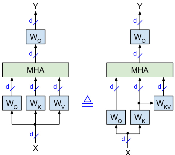
Figure 1: Mathematically identical implementations of multi-headed self-attention with square weight matrices $\in\mathbb{R}^{d\times d}$ . Left: vanilla version. Right: proposed version where values $\mathrm{v}$ are computed from keys K with $\bar{W_{K V}}=W_{K}^{-1}W_{V}$ . The $\triangleq$ symbol denotes mathematical identity.
图 1: 使用方形权重矩阵 $\in\mathbb{R}^{d\times d}$ 的多头自注意力机制在数学上等价的实现。左图:原始版本。右图:提出的版本,其中值 $\mathrm{v}$ 通过键 K 计算得出,且 $\bar{W_{K V}}=W_{K}^{-1}W_{V}$ 。符号 $\triangleq$ 表示数学上的等价性。
Slim attention is applicable to transformers that use MHA (multi-head attention [3]) instead of MQA (multi-query attention [4]) or GQA (grouped query attention [5]), which includes LLMs such as CodeLlama-7B and Aya-23-35B, SLMs such as Phi-3-mini and SmolLM2-1.7B, VLMs (vision language models) such as LLAVA, audio-language models such as Qwen2-Audio-7B, and encoder-decoder transformer models such as Whisper [6] and T5 [7]. Table 1 lists various MHA transformer models ranging from 9 million to 35 billion parameters. The last column of Table 1 specifies the KV-cache size (in number of activation s) for each model to support its maximum context length, where the KV-cache size equals $2h d_{k}$ · layers $\cdot$ context length.
Slim attention 适用于使用 MHA(多头注意力 [3])而非 MQA(多查询注意力 [4])或 GQA(分组查询注意力 [5])的 Transformer 模型,其中包括 CodeLlama-7B 和 Aya-23-35B 等大语言模型,Phi-3-mini 和 SmolLM2-1.7B 等小型语言模型,LLAVA 等视觉语言模型,Qwen2-Audio-7B 等音频语言模型,以及 Whisper [6] 和 T5 [7] 等编码器-解码器 Transformer 模型。表 1 列出了参数范围从 900 万到 350 亿的各种 MHA Transformer 模型。表 1 的最后一列指定了每个模型支持其最大上下文长度所需的 KV 缓存大小(以激活数表示),其中 KV 缓存大小等于 $2h d_{k}$ · 层数 $\cdot$ 上下文长度。
Table 1: Various transformers with MHA (instead of MQA or GQA) and their maximum KV-cache sizes (in number of activation s) based on their respective maximum context length. $h$ is the number of attention-heads, $d$ is the embedding dimension (aka hidden size), and $d_{k}$ is the head dimension. See appendix for more MHA models.
表 1: 使用 MHA (而非 MQA 或 GQA) 的各种 Transformer 及其基于各自最大上下文长度的最大 KV 缓存大小 (以激活数表示)。$h$ 是注意力头的数量,$d$ 是嵌入维度 (即隐藏大小),$d_{k}$ 是头维度。更多 MHA 模型请参见附录。
| 年份 | 发布者 | 模型 | 参数 | d | 层数 | h | dk | 上下文长度 | 上下文内存 |
|---|---|---|---|---|---|---|---|---|---|
| 2024 | Meta | CodeLlama-7B [8] | 7B | 4,096 | 32 | 128 | 16k | 4.3B | |
| CodeLlama-13B [8] | 13B | 5,120 | 40 | 6.7B | |||||
| CodeGemma-7B [9] | 8.5B | 3,072 | 28 | 16 | 256 | 8k | 1.9B | ||
| Cohere | Aya-23-35B [10] SmolLM2-1.7B [11] | 35B | 8,192 | 40 | 64 | 128 | 5.4B 0.8B | ||
| HuggingFace | SmolVLM [12] | 1.7B 2.3B | 2,048 | 24 | 32 | 64 | 16k | 1.6B | |
| Together AI | Evo-1-131k [13] | 6.5B | 4,096 | 32 | 128 | 128k | 34.4B | ||
| Microsoft | Phi-3-mini-128k [14] | 3.8B | 3,072 | 32 | 96 | 25.8B | |||
| Apple | BitNet_b1_58-3B [15] | 3.3B | 3,200 | 26 | 32 | 100 | 2k | 0.3B | |
| DCLM-7B [16] OLMo-1B [17] | 6.9B | 4,096 | 32 | 128 | 0.5B | ||||
| Ai2 | OLM0-2-1124-13B [17] | 1.3B 13.7B | 2,048 5,120 | 16 40 | 128 | 4k | 0.3B 1.7B | ||
| Amazon | Chronos-Bolt-tiny [18] | 9M | 256 | 4 | 64 | 0.5k | 1M | ||
| Alibaba | Chronos-Bolt-base [18] | 205M | 768 | 12 | 9.4M | ||||
| Qwen2-Audio-7B [19] | 8.4B | 4,096 | 32 | 8k | 2.1B | ||||
| LLaVA 2023 | LLaVA-NeXT-Video [20] | 7.1B | 128 | 4k | 1.1B | ||||
| LLaVA-Vicuna-13B [21] | 13.4B | 5,120 | 40 | 1.7B | |||||
| LMSYS | Vicuna-7B-16k [22] | 7B | 4,096 | 32 | 16k | 4.3B | |||
| Vicuna-13B-16k [22] | 13B | 5,120 | 40 | 6.7B | |||||
| Flan-T5-base [23] | 248M | 768 | 12 | 0.5k | 9.4M | ||||
| 2022 2019 | Flan-T5-XXL [23] | 11.3B | 4,096 | 24 | 64 | 101M | |||
| Whisper-tiny [6] | 38M | 384 | 4 | 6 | 64 | enc: 1500 dec: 448 | 6M | ||
| OpenAI | Whisper-large-v3 [6] GPT-2 XL [24] | 1.5B | 1,280 1,600 | 32 48 | 20 25 | 1k | 160M 157M |
For long contexts, the KV-cache can be even larger than the parameter memory: For batch size 1 and 1 byte (FP8) per parameter and activation, the Phi-3-mini $128\mathrm{k\Omega}$ model for example has a 3.8GB parameter memory and requires 25GB for its KV-cache to support a context length of 128K tokens. For a batch size of 16 for example, the KV-cache grows to $16\cdot25\mathrm{GB}=400\mathrm{GB}$ . Therefore, memory bandwidth and capacity become the bottleneck for supporting long context.
对于长上下文,KV缓存甚至可能比参数内存更大:例如,对于批量大小为1且每个参数和激活占用1字节(FP8)的情况,Phi-3-mini $128\mathrm{k\Omega}$ 模型的参数内存为3.8GB,而其KV缓存需要25GB来支持128K token的上下文长度。例如,当批量大小为16时,KV缓存将增长到 $16\cdot25\mathrm{GB}=400\mathrm{GB}$。因此,内存带宽和容量成为支持长上下文的瓶颈。
For a memory bound system with batch size 1, generating each token takes as long as reading all (activated) parameters and all KV-caches from memory. Therefore, slim attention can speed up the token generation by up to $2\mathbf{x}$ for long contexts. For the Phi-3-min $128\mathrm{k\Omega}$ model with 3.8GB parameters for example, slim attention reduces the KV-cache size from 25GB to 12.5GB, which reduces the total memory from 28.8GB to 16.3GB, and thus speeds up the token generation by up to $1.8\mathrm{x}$ for batch size 1 (the maximum speedup happens for the generation of the very last token of the 128K tokens). And for batch size 16 for example, the speedup is $(400{+}3.8)/\left(200{+}3.8\right){=}2\mathrm{x}$ .
对于批处理大小为1的内存受限系统,生成每个Token所需的时间与从内存中读取所有(激活的)参数和所有KV缓存的时间相当。因此,对于长上下文,slim attention可以将Token生成速度提升至多$2\mathbf{x}$。以Phi-3-min $128\mathrm{k\Omega}$模型为例,该模型有3.8GB的参数,slim attention将KV缓存大小从25GB减少到12.5GB,从而将总内存从28.8GB减少到16.3GB,并在批处理大小为1的情况下将Token生成速度提升至多$1.8\mathrm{x}$(最大加速发生在生成128K Token中的最后一个Token时)。而对于批处理大小为16的情况,加速比为$(400{+}3.8)/\left(200{+}3.8\right){=}2\mathrm{x}$。
The vanilla transformer [3] defines the self-attention $Y$ of input $X$ as follows, where $h$ is the number of heads:
普通的 Transformer [3] 将输入 $X$ 的自注意力 $Y$ 定义如下,其中 $h$ 是头的数量:

with $W_{Q}=\operatorname{concat}(W_{Q,1},\ldots,W_{Q,h})$ , $W_{K}=\operatorname{concat}(W_{K,1},\ldots,W_{K,h})$ , and $W_{V}=\operatorname{concat}(W_{V,1},\ldots,W_{V,h})$ , and without the causal mask for simplicity. The matrices $Q,K,V,W_{Q},W_{I}$ , and $W_{V}$ are split into $h$ sub matrices, one for each attention-head. Input $X$ , output $Y$ , queries $Q$ , keys $K$ , and values $V$ are $\in\mathbb{R}^{n\times d}$ , where $n$ is the current sequence length (in tokens) and $d=d_{\mathrm{model}}$ is the dimension of the embeddings.
其中 $W_{Q}=\operatorname{concat}(W_{Q,1},\ldots,W_{Q,h})$,$W_{K}=\operatorname{concat}(W_{K,1},\ldots,W_{K,h})$,以及 $W_{V}=\operatorname{concat}(W_{V,1},\ldots,W_{V,h})$,并且为了简化,省略了因果掩码。矩阵 $Q,K,V,W_{Q},W_{I}$ 和 $W_{V}$ 被分割成 $h$ 个子矩阵,每个子矩阵对应一个注意力头。输入 $X$,输出 $Y$,查询 $Q$,键 $K$ 和值 $V$ 都属于 $\mathbb{R}^{n\times d}$,其中 $n$ 是当前序列长度(以 token 为单位),$d=d_{\mathrm{model}}$ 是嵌入的维度。
For MHA, the weight matrices $W_{K}$ and $W_{V}$ are usually square matrices $\in\mathbb{R}^{d\times d}$ , which allows us to calculate $\mathrm{v}$ from K as follows: Refactoring equation (1) as $X=K W_{K}^{\bar{-}1}$ lets us reconstruct $X$ from $K$ , which we can then plug into equation (2) to get
对于 MHA (Multi-Head Attention) 来说,权重矩阵 $W_{K}$ 和 $W_{V}$ 通常是方阵 $\in\mathbb{R}^{d\times d}$,这使得我们可以从 $K$ 计算 $\mathrm{v}$ 如下:将方程 (1) 重构为 $X=K W_{K}^{\bar{-}1}$,我们可以从 $K$ 重构 $X$,然后将其代入方程 (2) 得到

and $W_{K V,i}\in\mathbb{R}^{d\times d_{v}}$ . Fig. 1 illustrates the modified attention scheme that calculates $\mathrm{v}$ from K according to equation (4). For inference, $W_{K V}=W_{K}^{-1}W_{V}$ can be pre computed offline and stored in the parameter file instead of $W_{V}$ . This requires that $W_{K}$ is invertible (i.e. non-singular). In general, any square matrix can be inverted if its determinant is non-zero. It’s extremely unlikely that a large matrix has a determinant that is exactly 0.
以及 $W_{K V,i}\in\mathbb{R}^{d\times d_{v}}$。图 1 展示了根据公式 (4) 从 K 计算 $\mathrm{v}$ 的改进注意力机制。在推理时,$W_{K V}=W_{K}^{-1}W_{V}$ 可以预先离线计算并存储在参数文件中,而不是 $W_{V}$。这要求 $W_{K}$ 是可逆的(即非奇异矩阵)。一般来说,任何方阵如果其行列式不为零,都可以被求逆。大型矩阵的行列式恰好为 0 的情况极为罕见。
Related work. Slim attention is somewhat similar to DeepSeek’s multi-head latent attention (MLA) [25]. Unlike MLA, slim attention is an exact post-training implementation of existing MHA models (including models with RoPE).
相关工作。Slim attention 与 DeepSeek 的多头潜在注意力(MLA)[25] 有些相似。与 MLA 不同的是,Slim attention 是对现有 MHA 模型(包括带有 RoPE 的模型)的精确训练后实现。
1 K-cache is all you need
1 K-cache 就是你所需要的一切
Inference consists of the following two phases, which are illustrated in Fig. 2 for the vanilla MHA with KV-cache, where $p$ is the number of input-tokens and $n$ is the total number of current tokens including input-tokens and generated tokens, so $n=p+1,\ldots,n_{m a x}$ and $n_{m a x}$ is the context window length:
推理包括以下两个阶段,如图 2 所示的带有 KV 缓存的普通 MHA (Multi-Head Attention) 模型,其中 $p$ 是输入 Token 的数量,$n$ 是当前 Token 的总数,包括输入 Token 和生成的 Token,因此 $n=p+1,\ldots,n_{m a x}$,且 $n_{m a x}$ 是上下文窗口的长度:
• During the prompt-phase (aka prefill phase), all $p$ input-tokens are batched up and processed in parallel. In this phase, the $\mathrm{K}$ and $\mathrm{v}$ projections are stored in the KV-cache. • During the generate-phase (aka decoding phase), each output-token is generated sequentially (aka autoregressively). For each iteration of the generate-phase, only one new $\mathbf{K}$ -vector and one new V-vector are calculated and stored in the KV-cache, while all the previously stored KV-vectors are read from the cache.
• 在提示阶段(也称为预填充阶段),所有 $p$ 个输入 Token 会被批量处理并并行计算。在此阶段,$\mathrm{K}$ 和 $\mathrm{V}$ 的投影会被存储在 KV 缓存中。
• 在生成阶段(也称为解码阶段),每个输出 Token 会依次生成(也称为自回归生成)。在生成阶段的每次迭代中,只会计算一个新的 $\mathbf{K}$ 向量和一个新的 V 向量,并将其存储在 KV 缓存中,同时从缓存中读取所有之前存储的 KV 向量。
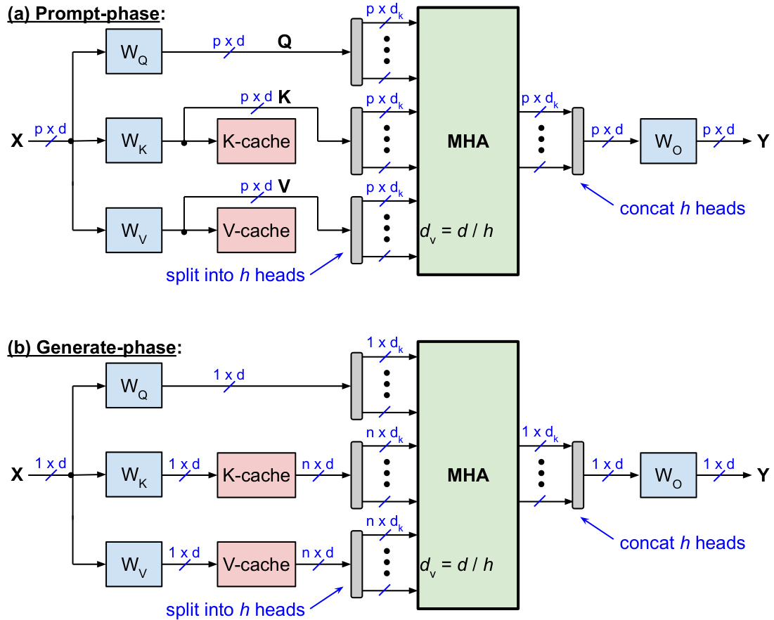
Figure 2: Standard MHA with KV-cache during (a) prompt-phase and (b) generate-phase.
图 2: 标准 MHA 在 (a) 提示阶段和 (b) 生成阶段使用 KV-cache 的情况。
Fig. 3 illustrates slim attention, which only has a K-cache because $\mathrm{v}$ is now calculated from K. Plugging equation (4) into (3) yields
图 3 展示了 slim attention,它只有一个 K-cache,因为 $\mathrm{v}$ 现在是从 K 计算得出的。将方程 (4) 代入 (3) 得到

Equation (5) can be computed in two different ways:
方程 (5) 可以通过两种不同的方式计算:
• Option 1 (un optimized): Compute $V_{i}=K W_{K V,i}$ first, and then multiply it with softmax $(\cdot)$ . This option is used by Fig. 3(a) and 3(b). Complexity: multiplying $K\in\mathbb{R}^{n\times d}$ with $W_{K V,i}\in\mathbb{R}^{d\times d_{k}}$ takes $2n d d_{k}\mathrm{OPs}^{2}$ , and multiplying softmax $(\cdot)\in\mathbb{R}^{1\times n}$ with the $n\times d_{k}$ result takes $2n d_{k}$ OPs.
• 选项 1 (未优化): 首先计算 $V_{i}=K W_{K V,i}$,然后将其与 softmax $(\cdot)$ 相乘。此选项用于图 3(a) 和 3(b)。复杂度:将 $K\in\mathbb{R}^{n\times d}$ 与 $W_{K V,i}\in\mathbb{R}^{d\times d_{k}}$ 相乘需要 $2n d d_{k}\mathrm{OPs}^{2}$,将 softmax $(\cdot)\in\mathbb{R}^{1\times n}$ 与 $n\times d_{k}$ 的结果相乘需要 $2n d_{k}$ OPs。
• Option 2 (optimized): First multiply softmax $(\cdot)$ with $K$ , and then multiply the result by $W_{K V,i}$ . This option is illustrated in Fig. 3(c). During the generate-phase, this option has lower compute complexity than option 1: multiplying softmax $(\cdot)$ with $K$ takes $2n d$ OPs, and multiplying the result with $W_{K V,i}$ takes $2d d_{k}$ OPs.
• 选项 2 (优化):首先将 softmax $(\cdot)$ 与 $K$ 相乘,然后将结果与 $W_{K V,i}$ 相乘。此选项如图 3(c) 所示。在生成阶段,此选项的计算复杂度低于选项 1:将 softmax $(\cdot)$ 与 $K$ 相乘需要 $2n d$ 次操作,将结果与 $W_{K V,i}$ 相乘需要 $2d d_{k}$ 次操作。
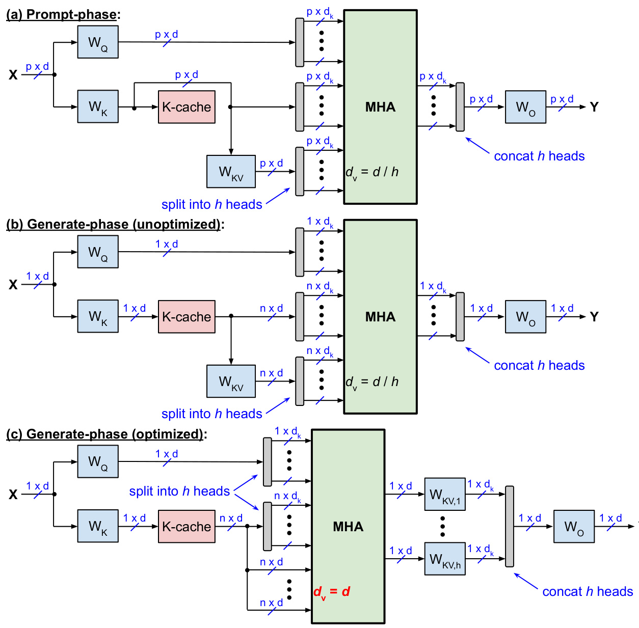
Option 2 Figure 3: Slim attention without V-cache during (a) prompt-phase; (b) un optimized and (c) optimized generate-phase
图 3: 无 V-cache 的 Slim attention 在 (a) 提示阶段;(b) 未优化和 (c) 优化生成阶段
Option 2 above uses the same associativity trick as MLA, see appendix C of [25]. During the prompt-phase, Fig. 3(a) has the same computational complexity as the vanilla scheme shown in Fig. 2(a). However, during the generate-phase, the proposed scheme has a slightly higher complexity than the vanilla scheme.
上述选项 2 使用了与 MLA 相同的结合性技巧,详见 [25] 的附录 C。在提示阶段,图 3(a) 的计算复杂度与图 2(a) 所示的原始方案相同。然而,在生成阶段,所提出的方案比原始方案的计算复杂度略高。
Table 2 specifies the complexity per token per layer during the generate-phase for batch size 1. The columns labeled “OPs”, “reads”, and “intensity” specify the computational complexity (as number of OPs), the number of memory reads, and the arithmetic intensity, resp. We define the arithmetic intensity here as number of OPs per each activation or parameter read from memory. Specifically, the projection complexity includes calculating $X W_{Q}$ , $X W_{K}$ , $X W_{V}$ , and multiplying with weight matrices $W_{O}$ and $W_{K V}$ . And the memory reads for projections include reading all four weight matrices; while the memory reads of the MHA include reading the K-cache (and the V-cache for the vanilla implementation). See appendix for more details on MHA complexity.
表 2 指定了在生成阶段(批次大小为 1)时每层每个 Token 的复杂度。标有“OPs”、“reads”和“intensity”的列分别指定了计算复杂度(以 OPs 的数量表示)、内存读取次数和算术强度。我们在这里将算术强度定义为每次从内存中读取激活值或参数时的 OPs 数量。具体来说,投影复杂度包括计算 $X W_{Q}$、$X W_{K}$、$X W_{V}$,以及与权重矩阵 $W_{O}$ 和 $W_{K V}$ 的乘法。投影的内存读取包括读取所有四个权重矩阵;而 MHA 的内存读取包括读取 K-cache(对于普通实现还包括 V-cache)。有关 MHA 复杂性的更多详细信息,请参阅附录。
Table 2: Complexity per token per layer during the generate-phase for batch size 1
表 2: 生成阶段每层每个 Token 的复杂度(批量大小为 1)
| 投影复杂度 | MHA 复杂度 | |||||
|---|---|---|---|---|---|---|
| OPs | reads | intensity | OPs | reads | intensity | |
| Vanilla,见图 2(b) | 8d² | 4d² | 2 | 4nd | 2nd | 2 |
| 未优化,图 3(b) | (2n + 6)d² | 4d² | (n + 3)/2 | 4nd | nd | 4 |
| 优化后,图 3(c) | 8d² | 4d² | 2 | 2nd(h + 1) | nd | 2h + 2 |
Note that for batch-size $B$ , the arithmetic intensity of the vanilla transformer during the generate-phase is $2B$ for the FFNs and the attention-projections, but only 2 for the remaining attention operations (softmax arguments and weighted sum of V) because each of the $B$ tokens has its own KV-cache.
请注意,对于批量大小 $B$,普通 Transformer 在生成阶段的算术强度对于 FFN 和注意力投影来说是 $2B$,但对于剩余的注意力操作(softmax 参数和 V 的加权求和)来说只有 2,因为每个 $B$ token 都有自己的 KV 缓存。
Table 3 shows the arithmetic intensity (now defined as OPs per memory byte) of various SoCs, TPUs, and GPUs, which vary from 93 to 583. A system is memory bound (i.e. limited by memory bandwidth) if the arithmetic intensity of the executed program is below the chip’s arithmetic intensity. Here, the maximum arithmetic intensity of slim attention is $2h+2$ , see Table 2, where $h$ is the number of attention-heads, which ranges between 16 and 64 for the models listed in Table 1. So the peak arithmetic intensity (up to 130 for $h=64$ ) is usually less than the system’s intensity (except for Apple’s $\mathbf{M}4\mathbf{M}\mathbf{a}\mathbf{x}$ ), which means that the system is still memory bound during the token generation phase. Therefore, slim attention speeds up the processing by up to $2\mathbf{x}$ as it reduces the context memory reads by half. Furthermore, slim attention enables processing all heads in parallel as a single matrix-matrix multiplication instead of multiple vector-matrix multiplications, which is usually more efficient and faster on many machines. And slim attention is also compatible with Flash Attention [26], which performs softmax and value accumulation in parallel.
表 3 展示了各种 SoC、TPU 和 GPU 的算术强度(现在定义为每内存字节的操作数),其范围从 93 到 583。如果执行程序的算术强度低于芯片的算术强度,则系统受内存限制(即受内存带宽限制)。在这里,slim attention 的最大算术强度为 $2h+2$,参见表 2,其中 $h$ 是注意力头的数量,表 1 中列出的模型的 $h$ 范围在 16 到 64 之间。因此,峰值算术强度(对于 $h=64$ 最高为 130)通常低于系统的强度(除了 Apple 的 $\mathbf{M}4\mathbf{M}\mathbf{a}\mathbf{x}$),这意味着在 token 生成阶段,系统仍然受内存限制。因此,slim attention 通过将上下文内存读取减少一半,将处理速度提高了最多 $2\mathbf{x}$。此外,slim attention 使得所有头可以并行处理,作为一个单一的矩阵-矩阵乘法,而不是多个向量-矩阵乘法,这在许多机器上通常更高效且更快。slim attention 还与 Flash Attention [26] 兼容,后者可以并行执行 softmax 和值累加。
Table 3: TOPS3, memory bandwidth, and arithmetic intensity of popular chips
表 3: 热门芯片的 TOPS3、内存带宽和算术强度
| 芯片 | TOPS (int8) | 理论内存带宽 (GB/s) | 算术强度 (每字节操作数) |
|---|---|---|---|
| Rockchip RK3588 | 6 | 19 | 316 |
| Apple A18 [27] | 35 | 60 | 583 |
| Apple M4 Max [27] | 38 | 410 | 93 |
| Google TPU v4 [28] | 275 | 1,200 | 229 |
| Google TPU v5p [28] | 918 | 2,765 | 332 |
| NVIDIA H200 [29] | 1,980 | 4,800 | 413 |
| NVIDIA B200 [29] | 4,500 | 8,000 | 563 |
2 Taking advantage of softmax sparsities
2 利用 softmax 的稀疏性
In this section we describe how we can take advantage of softmax sparsities (i.e. sparsities in the attention scores) to reduce the computational complexity of the attention blocks. In some applications, many attention scores are 0 or close to zero. For those attention scores (i.e. attention scores smaller than a threshold), we can simply skip the corresponding V-vector, i.e. we don’t have to add those skipped vectors to the weighted sum of V-vectors. This reduces the complexity of calculating the weighted sum of V-vectors. For example, for a sparsity factor $S=0.8$ (i.e. $80%$ of scores are 0), the complexity is reduced by factor 1−1S $\textstyle{\frac{1}{1-S}}=5$
在本节中,我们将描述如何利用 softmax 稀疏性(即注意力分数的稀疏性)来降低注意力模块的计算复杂度。在某些应用中,许多注意力分数为 0 或接近 0。对于那些注意力分数(即小于某个阈值的注意力分数),我们可以直接跳过相应的 V 向量,也就是说,我们不需要将这些跳过的向量添加到 V 向量的加权和中。这降低了计算 V 向量加权和的复杂度。例如,对于稀疏因子 $S=0.8$(即 $80%$ 的分数为 0),复杂度减少了 $1-\frac{1}{1-S}=5$ 倍。
By the way, taking advantage of softmax sparsities is also possible for systems with KV-cache where V is not computed from K. In this case, skipping $\mathrm{V}.$ -vectors with zero scores means that we don’t have to read those V-vectors from the KV-cache, which speeds up the auto regressive generate-phase for memory bound systems. However, this will never speed it up more than slim attention’s removal of the entire V-cache. Furthermore, for MQA and GQA, each V-vector is shared among multiple (e.g. 4 or more) queries so we can only skip reading a V-vector from memory if all 4 (or more) attention scores are zero for this shared ${\mathrm{V}}.$ -vector, which reduces the savings significantly. For example, if the V-vectors are shared among 4 queries and the attention scores have sparsity $S=0.8$ , then the probability of all four queries being 0 is only $S^{4}=\bar{0.4}1$ , so we can only skip $41%$ of the V-vectors.
顺便提一下,利用 softmax 的稀疏性对于具有 KV-cache 的系统也是可行的,其中 V 不是从 K 计算的。在这种情况下,跳过得分为零的 $\mathrm{V}.$ 向量意味着我们不需要从 KV-cache 中读取这些 V 向量,这可以加速内存受限系统的自回归生成阶段。然而,这永远不会比 slim attention 移除整个 V-cache 的速度更快。此外,对于 MQA 和 GQA,每个 V 向量在多个(例如 4 个或更多)查询之间共享,因此只有当所有 4 个(或更多)注意力得分对于这个共享的 ${\mathrm{V}}.$ 向量都为零时,我们才能跳过从内存中读取 V 向量,这会显著减少节省。例如,如果 V 向量在 4 个查询之间共享,并且注意力得分的稀疏性为 $S=0.8$,那么所有四个查询都为零的概率仅为 $S^{4}=\bar{0.4}1$,因此我们只能跳过 $41%$ 的 V 向量。
3Support for RoPE
3 对 RoPE 的支持
Many transformers nowadays use RoPE (rotary positional embedding) [30], which applies positional encoding to the Q and K projections, but not the V projections. In general, RoPE can be applied to the K projections either before storing them in K-cache or after reading them from K-cache. The former is preferred because of lower computational complexity during the generate-phase (so that each K-vector is RoPE’d only once instead of multiple times). However, if the RoPE’d keys are stored in K-cache, then we first need to un-RoPE them before we can compute V from K. The following details two options to support RoPE.
如今许多 Transformer 使用 RoPE (rotary positional embedding) [30],它将位置编码应用于 Q 和 K 的投影,但不应用于 V 的投影。通常,RoPE 可以在将 K 投影存储到 K-cache 之前或从 K-cache 读取之后应用于 K 投影。前者是首选,因为在生成阶段计算复杂度较低(因此每个 K 向量只被 RoPE 处理一次,而不是多次)。然而,如果 RoPE 处理后的键存储在 K-cache 中,那么在从 K 计算 V 之前,我们需要先对其进行反 RoPE 处理。以下详细介绍了支持 RoPE 的两种选项。
Option 1 is for the case where we don’t take advantage of softmax sparsities. In this case, we apply RoPE to the K-vectors after reading them from K-cache during the generate-phase. That way we can use the raw K-vectors for computing V from K.
选项 1 适用于我们不利用 softmax 稀疏性的情况。在这种情况下,我们在生成阶段从 K-cache 中读取 K 向量后,对它们应用 RoPE。这样我们就可以使用原始的 K 向量从 K 计算 V。
Option 2 is for the case where we take advantage of softmax sparsities as detailed in the previous section. In this case, RoPE is applied to the K-vectors before writing them into the K-cache. And when they are read from K-cache during the generate-phase, then we have to revert (or undo) the RoPE-encoding before we can use the K-vectors to compute the V-vectors (i.e. multiplying the K-vectors with the attention scores). However, we only need to do this for a portion of the K-vectors, depending on the sparsity factor $S$ . For example, for $S=0.8$ , we only need to revert the RoPE-encoding for $20%$ of the K-vectors. The RoPE encoding can be reverted (aka RoPE-decoding) by simply performing a rotation in the opposite direction by the same amount as shown below for the 2D case.
选项 2 适用于我们利用前一节中详述的 softmax 稀疏性的情况。在这种情况下,RoPE 在将 K 向量写入 K 缓存之前应用于它们。当在生成阶段从 K 缓存中读取它们时,我们必须先撤销(或反转)RoPE 编码,然后才能使用 K 向量来计算 V 向量(即将 K 向量与注意力分数相乘)。然而,我们只需要对一部分 K 向量执行此操作,具体取决于稀疏因子 $S$。例如,对于 $S=0.8$,我们只需要对 $20%$ 的 K 向量进行 RoPE 编码的反转。RoPE 编码可以通过简单地执行相反方向的旋转来反转(即 RoPE 解码),如下所示,以 2D 情况为例。
RoPE encoding:
RoPE编码:

RoPE decoding:
RoPE 解码:

Note that the RoPE decoding uses the same trigonometric coefficients (such as $\cos m\theta_{\scriptscriptstyle\perp}$ ) as the RoPE encoding. Therefore, we only need one look-up table that can be used for both RoPE encoding and decoding.
需要注意的是,RoPE 解码使用了与 RoPE 编码相同的三角函数系数(例如 $\cos m\theta_{\scriptscriptstyle\perp}$)。因此,我们只需要一个查找表,即可同时用于 RoPE 编码和解码。
4 Support for bias
4 对偏差的支持
Since PaLM’s removal of bias terms from all its projection layers [31], most transformer models nowadays do the same. However, some models are still using biases today (especially older models that are still relevant today such as Whisper). In this section, we briefly discuss how projection layers with bias can be supported. We show how the biases of two of the four attention projection layers can be eliminated in a mathematically equivalent way.
自 PaLM 从其所有投影层中移除偏置项 [31] 以来,现今大多数 Transformer 模型都采取了相同的做法。然而,一些模型至今仍在使用偏置项(尤其是至今仍具影响力的较旧模型,如 Whisper)。在本节中,我们简要讨论了如何支持带有偏置的投影层。我们展示了如何以数学上等价的方式消除四个注意力投影层中两个的偏置。
Bias removal for $\mathbf{V}$ projections: This bias can be combined with the bias of the output projection layer as follows. Recall that all value vectors $v_{i}$ plus their constant bias $b$ are multiplied by the attention scores $s_{i}$ (i.e. the softmax outputs) and summed up, such as
$\mathbf{V}$ 投影的偏差去除:这种偏差可以与输出投影层的偏差结合如下。回想一下,所有的值向量 $v_{i}$ 加上它们的常数偏差 $b$ 都会乘以注意力分数 $s_{i}$(即 softmax 输出)并求和,例如

The last equal sign holds because the sum over all attention-scores $s_{i}$ is always 1 as per softmax definition (because the softmax generates a probability distribution that always adds up to 1). We can now merge the bias $b$ with bias $c$ of the
最后一个等号成立是因为根据 softmax 的定义,所有注意力分数 $s_{i}$ 的总和始终为 1(因为 softmax 生成的概率分布总和始终为 1)。我们现在可以将偏差 $b$ 与偏差 $c$ 合并。
preceding output projection layer (O) as follows: $y=(x+b)W_{O}+c=x W_{O}+(b W_{O}+c)=x W_{O}+c^{}$ , with the new bias $c^{}=b W o+c$ . This new bias-vector $c^{*}$ can be computed offline, before inference time. Or simply remove the V-bias already during training.
前面的输出投影层 (O) 如下:$y=(x+b)W_{O}+c=x W_{O}+(b W_{O}+c)=x W_{O}+c^{}$,其中新的偏置 $c^{}=b W o+c$。这个新的偏置向量 $c^{*}$ 可以在推理时间之前离线计算。或者简单地在训练期间移除 V-bias。
Bias removal for $\mathbf{K}$ projections: The bias of the $\mathbf{K}$ projection cancels out due to the constant invariance of the softmax function. For example, say we have 2-dimensional heads, then the dot-product $p$ between query-vector $q=(q_{1}+b_{1},q_{2}+b_{2})$ with bias $b$ and key-vector $\boldsymbol{k}=\left(k_{1}+c_{1},k_{2}+c_{2}\right)$ with bias $c$ is as follows:
$\mathbf{K}$ 投影的偏差消除:由于 softmax 函数的常数不变性,$\mathbf{K}$ 投影的偏差会被抵消。例如,假设我们有二维的注意力头,那么带有偏差 $b$ 的查询向量 $q=(q_{1}+b_{1},q_{2}+b_{2})$ 和带有偏差 $c$ 的键向量 $\boldsymbol{k}=\left(k_{1}+c_{1},k_{2}+c_{2}\right)$ 之间的点积 $p$ 如下:

where $f(q)=q_{1}c_{1}+q_{2}c_{2}$ is a function of the query-vector only; and “constant” is a constant that only depends on the two biases $b$ and $c$ . Now recall that the softmax function doesn’t change if a constant is added to all its arguments. Because all arguments of the attention softmax use the same single query-vector $q$ , $f(q)$ is the same for all arguments and is therefore constant and can be removed from all softmax arguments. As a result, we can remove the entire bias-vector $c$ from the keys. But we still need the bias-vector $b$ for the queries. However, this assumes that there is no RoPE applied between the projections and the dot-product calculation, which is fortunately the case for Whisper for example.
其中 $f(q)=q_{1}c_{1}+q_{2}c_{2}$ 是一个仅与查询向量相关的函数;而“constant”是一个仅依赖于两个偏置 $b$ 和 $c$ 的常数。现在回想一下,softmax 函数在其所有参数上加上一个常数时不会改变。由于注意力 softmax 的所有参数都使用相同的查询向量 $q$,$f(q)$ 对所有参数都是相同的,因此可以视为常数,可以从所有 softmax 参数中移除。因此,我们可以从键中移除整个偏置向量 $c$。但我们仍然需要偏置向量 $b$ 用于查询。然而,这假设在投影和点积计算之间没有应用 RoPE(旋转位置编码),幸运的是,例如 Whisper 就是这种情况。
5 Support for non-square weight matrices
5 支持非方形权重矩阵
Some transformers with MHA use non-square weight matrices for their K and $\mathrm{v}$ projections. Specifically, these models do not satisfy $d=d_{k}h$ . The table below shows three such models where $e=d_{k}h>d$ . Let’s also define the aspect ratio $r$ as $r=e/d$ . For example, Google’s T5-11B model has a large aspect ratio of $r=16$ .
一些使用多头注意力机制 (MHA) 的 Transformer 在其 K 和 $\mathrm{v}$ 投影中使用了非方阵权重矩阵。具体来说,这些模型不满足 $d=d_{k}h$。下表展示了三个这样的模型,其中 $e=d_{k}h>d$。我们还可以定义长宽比 $r$ 为 $r=e/d$。例如,Google 的 T5-11B 模型的长宽比很大,为 $r=16$。
| 模型 | d | dk | h | e=dkh | 宽高比 r = e/d |
|---|---|---|---|---|---|
| CodeGemma-7B | 3,072 | 256 | 16 | 4,096 | 1.3 |
| T5-3B | 1,024 | 128 | 32 | 4,096 | 4 |
| T5-11B | 1,024 | 128 | 128 | 16,384 | 16 |
There are two options to reduce the KV-cache by $2\mathbf{x}$ or more, which are compared in the table below and summarized as follows:
有两种方法可以将 KV-cache 减少 $2\mathbf{x}$ 或更多,下表对其进行了比较并总结如下:
• Option 1: Because the K weight matrix is non-square, inverting this matrix is not straight forward. And the resulting matrix $W_{K V}\in\mathbb{R}^{e\times e}$ , which has $r$ -times more parameters than $W_{V}\in\mathbb{R}^{d\times e}$ . • Option 2: Instead of storing $\mathrm{v}$ in cache and then calculating $\mathrm{v}$ from K, we can store the smaller $d$ -element vectors $\boldsymbol{\mathrm X}$ before the projection and then on-the-fly calculate both projections ( $\mathrm{V}$ and K) from X. The cache is now $r$ -times smaller than option 1, and $2r$ times smaller than the baseline, for example 32 times smaller for the T5-11B model. However, this comes at a slightly higher computational cost.
• 选项 1:由于 K 权重矩阵是非方阵,因此求逆矩阵并不直接。生成的矩阵 $W_{K V}\in\mathbb{R}^{e\times e}$ 比 $W_{V}\in\mathbb{R}^{d\times e}$ 多出 $r$ 倍的参数。
• 选项 2:与其将 $\mathrm{v}$ 存储在缓存中,然后从 K 计算 $\mathrm{v}$,我们可以在投影之前存储较小的 $d$ 元素向量 $\boldsymbol{\mathrm X}$,然后动态地从 X 计算两个投影($\mathrm{V}$ 和 K)。现在缓存比选项 1 小 $r$ 倍,比基线小 $2r$ 倍,例如对于 T5-11B 模型来说,缓存小了 32 倍。然而,这会带来稍高的计算成本。
| Baseline | Option 1 | Option 2 | |
|---|---|---|---|
| 缓存减少因子 | 1 | 2 | 2r |
| Wv 或 Wkv 的大小 | de | e2 (r 倍大) | de |
| 计算复杂度 | baseline | 更高 | 更高 |
| 支持 RoPE? | 是 | 是 | 否 |
Option 1: The standard matrix inverse is defined only for square matrices, and the inversion functions in NumPy and SciPy are limited to such matrices. We want to compute the inverse of $W_{K}\in\mathbb{R}^{d\times e}$ with $e>d$ such that $W_{K}W_{K}^{-1}=I$ , where $I$ is the identity matrix and $W_{K}^{-1}$ is the so-called right inverse of $W_{K}$ . We compute $W_{K}^{-1}$ by using a trick that inverts the term $W_{K}W_{K}^{\top}$ instead of $W_{K}$ as follows:
选项 1:标准矩阵逆仅针对方阵定义,NumPy 和 SciPy 中的逆函数也仅限于此类矩阵。我们希望计算 $W_{K}\in\mathbb{R}^{d\times e}$ 的逆矩阵,其中 $e>d$,使得 $W_{K}W_{K}^{-1}=I$,其中 $I$ 是单位矩阵,$W_{K}^{-1}$ 是 $W_{K}$ 的所谓右逆矩阵。我们通过使用一个技巧来计算 $W_{K}^{-1}$,即对 $W_{K}W_{K}^{\top}$ 进行逆运算,而不是直接对 $W_{K}$ 进行逆运算,具体如下:

In the equation above, everything on the right side of $W_{K}$ has to be the inverse of $W_{K}$ , thus $W_{K}^{-1}=W_{K}^{\top}(W_{K}W_{K}^{\top})^{-1}$ . We can now use the matrix inversion function of NumPy to compute the inverse of the term $W_{K}W_{K}^{\top}$ , which is a square $d\times d$ matrix. Now we can calculate $W_{K V}=W_{K}^{-1}W_{V}$ . However, storing $W_{K V}$ instead of the original $W_{V}$ takes $r$ times more space in memory, which is an issue for large aspect-ratios $r$ .
在上面的等式中,$W_{K}$ 右侧的所有内容都必须是 $W_{K}$ 的逆矩阵,因此 $W_{K}^{-1}=W_{K}^{\top}(W_{K}W_{K}^{\top})^{-1}$。我们现在可以使用 NumPy 的矩阵求逆函数来计算 $W_{K}W_{K}^{\top}$ 的逆矩阵,这是一个 $d\times d$ 的方阵。现在我们可以计算 $W_{K V}=W_{K}^{-1}W_{V}$。然而,存储 $W_{K V}$ 而不是原始的 $W_{V}$ 会占用 $r$ 倍的内存空间,这对于大宽高比 $r$ 来说是一个问题。
Option 2 caches the $\mathrm{X}$ -matrix instead of KV or just K, where the $\mathrm{X}$ -matrix contains the input activation s of the attention layer (before the projections). Re computing all K-vectors from $\boldsymbol{\mathrm X}$ by multiplying $\boldsymbol{\mathrm X}$ with weight matrix $W_{K}$ would require 2nde operations and would be very expensive. A lower complexity option is illustrated in Fig. 4, which is similar to the trick illustrated in Fig. 3(c). Recall that for the $i$ -th head $(i=1,\ldots,h)$ , the softmax argument (without the scaling factor $1/\sqrt{d_{k}})$ is $A_{i}=Q_{i}K_{i}^{\top}$ , where $Q_{i}=X W_{Q,i}$ and $K_{i}=X W_{K,i}$ . For the generate-phase, there is only one input-vector $x_{n}$ for the query, but there are $n$ input-vectors $X$ for the key and value projections. We can take advantage of this and modify $A$ as follows (which uses the trick $\left(B C\right)^{\top}=C^{\top}\dot{B}^{\top}$ for transposing the product of arbitrary matrices $B$ and $C$ ):
选项 2 缓存的是 $\mathrm{X}$ 矩阵,而不是 KV 或仅仅是 K,其中 $\mathrm{X}$ 矩阵包含注意力层的输入激活(在投影之前)。通过将 $\boldsymbol{\mathrm X}$ 与权重矩阵 $W_{K}$ 相乘来重新计算所有 K 向量需要 2nde 次操作,这将非常昂贵。图 4 展示了一个复杂度较低的选项,类似于图 3(c) 中的技巧。回想一下,对于第 $i$ 个头 $(i=1,\ldots,h)$,softmax 参数(不包括缩放因子 $1/\sqrt{d_{k}})$ 是 $A_{i}=Q_{i}K_{i}^{\top}$,其中 $Q_{i}=X W_{Q,i}$ 和 $K_{i}=X W_{K,i}$。在生成阶段,查询只有一个输入向量 $x_{n}$,但键和值投影有 $n$ 个输入向量 $X$。我们可以利用这一点并修改 $A$ 如下(使用 $\left(B C\right)^{\top}=C^{\top}\dot{B}^{\top}$ 的技巧来转置任意矩阵 $B$ 和 $C$ 的乘积):
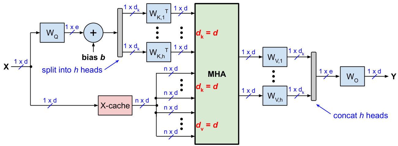
Figure 4: Slim attention with $\mathrm{X}$ -cache (instead of KV or V-cache) for the generate-phase of transformers with non-square weight matrices with $e>d$ .
图 4: 使用 $\mathrm{X}$ -cache(而非 KV 或 V-cache)的 Slim attention,适用于具有非方形权重矩阵($e>d$)的 Transformer 生成阶段。

For each iteration of the generate-phase, we now have to calculate the term $x_{n}W_{Q,i}W_{K,i}^{\top}$ only once for each attentionhead, which is independent of the sequence length. Calculating this term involves multiplying the $d$ -dimensional vector $x_{n}$ with matrices $W_{Q,i}\in\mathbb{R}^{d\times d_{k}}$ and $W_{K,i}^{\top}\in\mathbb{R}^{d_{k}\times d}$ , which requires $2d e$ multiplications for the $h$ heads, so $4d e$ operations in total (where we count a multiply-add operation as 2 operations).
在生成阶段的每次迭代中,我们现在只需为每个注意力头计算一次 $x_{n}W_{Q,i}W_{K,i}^{\top}$ 项,这与序列长度无关。计算该项涉及将 $d$ 维向量 $x_{n}$ 与矩阵 $W_{Q,i}\in\mathbb{R}^{d\times d_{k}}$ 和 $W_{K,i}^{\top}\in\mathbb{R}^{d_{k}\times d}$ 相乘,这需要为 $h$ 个头进行 $2d e$ 次乘法,因此总共需要 $4d e$ 次操作(我们将一次乘加操作计为 2 次操作)。
This scheme also works for projection layers with biases (as used by the Whisper models for example). Recall from the previous section that we can eliminate the biases from the key and value projections, but not from the query projection. Adding a constant query bias-vector $b$ to the equation above is straightforward and also illustrated in Fig. 4:
该方案也适用于带有偏置的投影层(例如 Whisper 模型所使用的)。回顾上一节,我们可以消除键和值投影中的偏置,但不能消除查询投影中的偏置。在上述方程中添加一个常数查询偏置向量 $b$ 是直接的,如图 4 所示:

However, this scheme doesn’t work if there is a positional encoding such as RoPE located between the projection layers and the dot-product calculation. But option 2 fully supports other relative position encoding (PE) schemes such as RPE of the T5 model, Alibi, Kerple and FIRE [32] which add a variable bias to the softmax arguments (instead of modifying the queries and keys before the dot-product calculation). See for example the FIRE paper [32], which shows that FIRE and even NoPE can outperform RoPE for long context.
然而,如果投影层和点积计算之间存在诸如 RoPE 的位置编码,此方案将无法工作。但选项 2 完全支持其他相对位置编码 (PE) 方案,例如 T5 模型的 RPE、Alibi、Kerple 和 FIRE [32],这些方案向 softmax 参数添加了一个可变偏差(而不是在点积计算之前修改查询和键)。例如,参见 FIRE 论文 [32],该论文表明,对于长上下文,FIRE 甚至 NoPE 可以优于 RoPE。
6 Support for encoder-decoder transformers
6 支持编码器-解码器 Transformer
In general, calculating K from V is not only possible for self-attention (see Fig. 1) but also for cross-attention. In this section, we present two context memory options for encoder-decoder transformers such as Whisper (speech-to-text), language translation models such as Google’s T5, and time series forecasting models such as Amazon’s Chronos models. One option is not limited to MHA only, but is also applicable to MQA and GQA. The table below compares the options, which are summarized as follows:
一般来说,从 V 计算 K 不仅适用于自注意力机制(见图 1),也适用于交叉注意力机制。在本节中,我们为编码器-解码器 Transformer(如 Whisper(语音转文本))、语言翻译模型(如 Google 的 T5)以及时间序列预测模型(如 Amazon 的 Chronos 模型)提供了两种上下文记忆选项。其中一个选项不仅限于多头注意力机制 (MHA),还适用于多查询注意力机制 (MQA) 和分组查询注意力机制 (GQA)。下表比较了这些选项,总结如下:
• The baseline implementation uses complete KV-caches for both self-attention and cross-attention of the decoder stack, which we refer to as self KV-cache and cross KV-cache, resp.
• 基线实现为解码器堆栈的自注意力(self-attention)和交叉注意力(cross-attention)使用了完整的KV缓存(KV-cache),我们分别称之为自KV缓存(self KV-cache)和交叉KV缓存(cross KV-cache)。
• Option 1 is an optimized implementation where the V-caches for both self-attention and cross-attention are eliminated, which reduces the total cache size by 2x. • Option 2 eliminates the entire cross KV-cache and also eliminates the V-cache of the self-attention.
- 选项 1 是一种优化实现,其中消除了自注意力 (self-attention) 和交叉注意力 (cross-attention) 的 V-cache,从而将总缓存大小减少 2 倍。
- 选项 2 消除了整个交叉 KV-cache,同时也消除了自注意力的 V-cache。
The baseline implementation consists of the following three phases:
基线实现包括以下三个阶段:
• During the prompt-phase, only the encoder is active. All $p$ input-tokens are batched up and processed in parallel. This phase is identical to the prompt-phase of a decoder-only transformer albeit without a causal mask (and is also identical to the entire inference of an encoder-only transformer such as BERT). • During the cross-phase, we take the output of the encoder (which is a $p\times d$ matrix) and precompute the KV projections for the decoder’s cross-attention and store them in cross context memory (aka cross KV-cache). • The generate-phase is similar to the generate-phase of a decoder-only transformer with the following difference: There is a cross-attention block for each layer, which reads keys and values from the cross KVcache. In addition, the self-attention blocks have their own self KV-cache (which is not the same as the cross KV-cache).
• 在提示阶段 (prompt-phase),只有编码器处于活动状态。所有 $p$ 个输入 token 被批量处理并并行处理。此阶段与仅解码器 Transformer 的提示阶段相同,只是没有因果掩码 (causal mask)(并且与仅编码器 Transformer(如 BERT)的整个推理过程相同)。
• 在交叉阶段 (cross-phase),我们获取编码器的输出(这是一个 $p\times d$ 的矩阵),并预先计算解码器交叉注意力 (cross-attention) 的 KV 投影,并将其存储在交叉上下文内存(也称为交叉 KV 缓存 (cross KV-cache))中。
• 生成阶段 (generate-phase) 与仅解码器 Transformer 的生成阶段类似,但有如下区别:每一层都有一个交叉注意力块,它从交叉 KV 缓存中读取键和值。此外,自注意力块 (self-attention blocks) 有自己的自 KV 缓存 (self KV-cache)(这与交叉 KV 缓存不同)。
| 基线 (Baseline) | 选项 1 (Option 1) | 选项 2 (Option 2) | |
|---|---|---|---|
| SelfKV 缓存大小 (SelfKV-cachesize) | 100% | 50% | 50% |
| CrossKV 缓存大小 (CrossKV-cachesize) | 100% | 50% | 0 |
| 生成阶段是否需要读取 cross-Wk 和 Wy? | 否 | 仅 Wkv | AM pue XM |
| 是否支持 RoPE? | 是 | 是 | 否 |
| 跨阶段复杂度 (Complexity of cross-phase) | 完整 | 一半 | 0 |
Option 1 calculates $\mathrm{v}$ from K for both self-attention and cross-attention of the decoder stack (note that the encoder stack doesn’t have a KV-cache because it is not auto regressive). This requires reading the cross $W_{K V}$ parameters from memory during the generate-phase. So if the $W_{K V}$ matrices are larger than the cross V-cache, then calculating $\mathrm{v}$ from K for the cross-attention doesn’t make sense for batch size 1 (but for larger batch sizes). For the Whisper models for example, the cross V-cache is always larger than the $W_{K V}$ matrices, because the number of encoder-tokens $p$ is always 1500. And for batch sizes $B$ larger than 1, the reading of the cross $W_{K V}$ parameters can be amortized among the $B$ inferences.
选项 1 从 K 计算 $\mathrm{v}$,用于解码器堆栈的自注意力和交叉注意力(注意,编码器堆栈没有 KV 缓存,因为它不是自回归的)。这需要在生成阶段从内存中读取交叉 $W_{K V}$ 参数。因此,如果 $W_{K V}$ 矩阵大于交叉 V 缓存,那么对于批量大小为 1 的情况,从 K 计算 $\mathrm{v}$ 用于交叉注意力是没有意义的(但对于更大的批量大小则不然)。例如,对于 Whisper 模型,交叉 V 缓存总是大于 $W_{K V}$ 矩阵,因为编码器 Token 的数量 $p$ 总是 1500。对于批量大小 $B$ 大于 1 的情况,交叉 $W_{K V}$ 参数的读取可以在 $B$ 次推理中分摊。
Option 2 efficiently recomputes the cross KV-projections from the encoder output instead of storing them in the cross KV-cache as follows:
选项 2 高效地从编码器输出中重新计算交叉 KV 投影,而不是将它们存储在交叉 KV 缓存中,具体如下:
Time-to-first-token (TTFT): Options 1 and 2 speed up or eliminate the cross-phase. Specifically, option 1 speeds up the cross-phase by $2\mathbf{x}$ . And option 2 completely eliminates the cross-phase. This speeds up the time-to-first-token latency (TTFT). And in certain cases, the overall compute complexity can be reduced compared to the baseline. For cases where the number of encoder-tokens is larger than the decoder-tokens (such as for Whisper or for text sum mari z ation) and for large $d$ dimensions, these options can reduce the overall complexity.
首 Token 时间 (TTFT):选项 1 和选项 2 加速或消除了跨阶段。具体来说,选项 1 将跨阶段加速了 $2\mathbf{x}$。而选项 2 则完全消除了跨阶段。这加速了首 Token 时间 (TTFT) 的延迟。在某些情况下,与基线相比,整体计算复杂度可以降低。对于编码器 Token 数量大于解码器 Token 数量的情况(例如 Whisper 或文本摘要),以及对于较大的 $d$ 维度,这些选项可以降低整体复杂度。

Figure 5: Slim attention with a single $\mathrm{X}$ -cache that is shared among all cross-attention layers for the generate-phase of encoder-decoder transformers.
图 5: 使用单个 $\mathrm{X}$ -缓存的精简注意力机制,该缓存在编码器-解码器 Transformer 的生成阶段的所有交叉注意力层之间共享。
The table below lists the cache size savings and speedups during the generate-phase for all 5 Whisper models, assuming a fixed encoder context length of $p=1500$ , a decoder output context length of 448, and a vocab_size of 51,865. Option 2 reduces the cache sizes by $8.7\mathbf{X}$ , assuming that the entire encoder output (matrix E) is kept in on-chip SRAM (the E-cache), which speeds up the generate-phase by over ${5}\mathbf{{X}}$ for a memory bound system with batch size 64. Note that the speedups listed in the table are in addition to speeding up the cross-phase (i.e. $2\mathbf{x}$ cross-phase speedup for option 1, and entire elimination of the cross-phase for option 2).
下表列出了所有 5 种 Whisper 模型在生成阶段的缓存大小节省和加速情况,假设固定的编码器上下文长度为 $p=1500$,解码器输出上下文长度为 448,词汇表大小为 51,865。假设整个编码器输出(矩阵 E)保存在片上 SRAM(E-cache)中,选项 2 将缓存大小减少了 $8.7\mathbf{X}$,对于批大小为 64 的内存受限系统,生成阶段加速超过 ${5}\mathbf{{X}}$。请注意,表中列出的加速是在加速交叉阶段(即选项 1 的交叉阶段加速 $2\mathbf{x}$,选项 2 完全消除了交叉阶段)的基础上进行的。
There is a further optimization, which is a hybrid of options 1 and 2, where one layer of the decoder stack uses option 1 and the other layers use a modified version of option 2 as follows: Say the first layer implements option 1, which entails calculating and storing the cross K-cache for the first layer, i.e. $K=E W_{K}$ . The trick is now to use this K-cache instead of the E-cache for all the other layers and then we can calculate E from K as $E=K W_{K_l a y e r1}^{-1}$ W K−_1layer1. So the other layers will now use K instead of E, which means that they need to use modified versions of their $W_{K}$ and $W_{V}$ weight matrices, which are offline computed as $W_{V_n e w}=W_{K_l a y e r1}^{-1}W_{V_o l d}$ W K−_1layer1WV _old and WK_new = W K−_1la $W_{K_n e w}=W_{K_l a y e r1}^{-1}W_{K_o l d}$ yer1WK_old. The savings of this hybrid versus option 2 are not huge: It only speeds up the first layer because we only need to read one of the two cross weight matrices for the first layer for each generated token (i.e. we only need to read $W_{K V_l a y e r1}$ instead of reading both $W_{K_l a y e r1}$ and $W_{V_l a y e r1})$ . So this hybrid makes only sense for shallow models, e.g. Whisper tiny which only has 4 layers.
还有一种进一步的优化方案,它是选项 1 和选项 2 的混合体,其中解码器堆栈的一层使用选项 1,其他层使用修改后的选项 2 版本,具体如下:假设第一层实现了选项 1,这意味着需要计算并存储第一层的交叉 K 缓存,即 $K=E W_{K}$。现在的技巧是使用这个 K 缓存而不是 E 缓存用于所有其他层,然后我们可以从 K 计算 E 为 $E=K W_{K_l a y e r1}^{-1}$ W K−_1layer1。因此,其他层现在将使用 K 而不是 E,这意味着它们需要使用修改后的 $W_{K}$ 和 $W_{V}$ 权重矩阵,这些矩阵离线计算为 $W_{V_n e w}=W_{K_l a y e r1}^{-1}W_{V_o l d}$ W K−_1layer1WV _old 和 WK_new = W K−_1la $W_{K_n e w}=W_{K_l a y e r1}^{-1}W_{K_o l d}$ yer1WK_old。这种混合方案相对于选项 2 的节省并不大:它只加速了第一层,因为对于每个生成的 token,我们只需要读取第一层的两个交叉权重矩阵中的一个(即我们只需要读取 $W_{K V_l a y e r1}$ 而不是同时读取 $W_{K_l a y e r1}$ 和 $W_{V_l a y e r1})$。因此,这种混合方案仅对浅层模型有意义,例如只有 4 层的 Whisper tiny。
7 Conclusion
7 结论
Slim attention offers a simple trick for halving the context memory of existing MHA transformer models without sacrificing accuracy. Slim attention is a post-training, exact implementation of existing models, so it doesn’t require any fine-tuning or training from scratch. Future work includes integrating slim attention into popular frameworks such as Hugging Face Transformers [33], llama.cpp [34], vLLM [35], llamafile [36], LM Studio [37], Ollama [38], SGLang [39], and combining it with existing context memory management schemes such as Paged Attention [40] and other compression schemes such as Dynamic Memory Compression DMC [41] and VL-cache [42]. Please also see our forthcoming paper about matrix-shrink [43], which reduces the sizes of attention matrices and proposes a simplification of DeepSeek’s MLA scheme.
Slim attention 提供了一种简单的技巧,可以在不牺牲准确性的情况下,将现有 MHA Transformer 模型的上下文内存减半。Slim attention 是对现有模型进行训练后的精确实现,因此不需要任何微调或从头开始训练。未来的工作包括将 slim attention 集成到流行的框架中,例如 Hugging Face Transformers [33]、llama.cpp [34]、vLLM [35]、llamafile [36]、LM Studio [37]、Ollama [38]、SGLang [39],并将其与现有的上下文内存管理方案(如 Paged Attention [40])和其他压缩方案(如动态内存压缩 DMC [41] 和 VL-cache [42])结合。请参阅我们即将发表的关于 matrix-shrink [43] 的论文,该论文减少了注意力矩阵的大小,并提出了对 DeepSeek 的 MLA 方案的简化。
Acknowledgments
致谢
We would like to thank Dirk Groeneveld (Ai2) and Zhiqiang Xie (Stanford, SGLang) for helpful discussions on this work. We are particularly grateful to Noam Shazeer for his positive feedback on slim attention. And special thanks to Imo Udom, Mitchell Baker, and Mozilla for supporting this work.
我们要感谢 Dirk Groeneveld (Ai2) 和 Zhiqiang Xie (斯坦福大学, SGLang) 对这项工作的有益讨论。我们特别感谢 Noam Shazeer 对 slim attention 的积极反馈。同时,特别感谢 Imo Udom、Mitchell Baker 和 Mozilla 对这项工作的支持。
| Whisper 模型 | tiny | base | small | medium | large | 备注 |
|---|---|---|---|---|---|---|
| 参数量 (Params) | 38M | 73M | 242M | 764M | 1.5B | 参数数量 |
| 层数 (Layers) | 4 | 6 | 12 | 24 | 32 | 层数 |
| p | 384 | 512 | 768 | 1,024 | 1,280 | 嵌入维度 |
| dffn | 1,536 | 2,048 | 3,072 | 4,096 | 5,120 | FFN 隐藏维度 |
| 缓存大小 (Cache sizes) (单位: M): | ||||||
| 编码器 E-cache (Encoder E-cache) | 0.6 | 0.8 | 1.2 | 1.5 | 1.9 | 1500·d |
| 交叉 KV-cache (Cross KV-cache) | 4.6 | 9.2 | 27.6 | 73.7 | 122.9 | 2·1500 ·d · layers |
| 自 KV-cache (Self KV-cache) | 1.4 | 2.8 | 8.3 | 22.0 | 36.7 | 2 · 448 · d · layers |
| 基线缓存 (Baseline cache) | 6.0 | 12.0 | 35.9 | 95.7 | 159.6 | 交叉 KV + 自 KV |
| 选项 1 缓存 (Option 1 cache) | 3.0 | 6.0 | 18.0 | 47.9 | 79.8 | 基线的一半 |
| 选项 2 缓存 (Option 2 cache) | 0.7 | 1.4 | 4.1 | 11.0 | 18.4 | 无交叉 KV + 自 KV-cache 的一半 |
| 选项 2 节省 (Option 2 savings) | 8.7x | 8.7x | 8.7x | 8.7x | 8.7x | 缓存节省 vs. 基线 |
| 生成阶段参数量 (Number of parameters) (单位: M): | ||||||
| 基线参数量 (Baseline params) | 28.2 | 48.6 | 138.9 | 405.4 | 800.4 | d · vocab + layers · (6d? + 2d · dfn) |
| 选项 1 参数量 (Option 1 params) | 28.8 | 50.1 | 146.0 | 430.6 | 852.8 | 基线 + 交叉 K (d? · layers) |
| 选项 2 参数量 (Option 2 params) | 29.4 | 51.7 | 153.1 | 455.8 | 905.2 | 基线 + 交叉 KV (2d2 · layers) |
| 每 Token 内存读取量 (Memory reads) (单位: M) (批量大小 1): | ||||||
| 基线 (Baseline) | 34.2 | 60.5 | 174.8 | 501.2 | 960.0 | 基线缓存 + 基线参数量 |
| 选项 1 (Option 1) | 31.8 | 56.1 | 164.0 | 478.5 | 932.6 | 选项 1 缓存 + 选项 1 参数量 |
| 选项 2 (Option 2) | 30.0 | 53.1 | 157.2 | 466.8 | 923.6 | 选项 2 缓存 + 选项 2 参数量 |
| 选项 1 加速 (Option 1 speedup) | 1.08x | 1.08x | 1.07x | 1.05x | 1.03x | 加速 vs. 基线 |
| 选项 2 加速 (Option 2 speedup) | 1.14x | 1.14x | 1.11x | 1.07x | 1.04x | 加速 vs. 基线 |
| 每 Token 内存读取量 (Memory reads) (单位: M) (批量大小 64): | ||||||
| 基线 (Baseline) | 6.4 | 12.7 | 38.1 | 102.1 | 172.1 | 基线缓存 + 1/64· 参数量 |
| 选项 1 (Option 1) | 3.4 | 6.8 | 20.2 | 54.6 | 93.1 | 选项 1 缓存 + 1/64· 参数量 |
| 选项 2 (Option 2) | 1.1 | 2.2 | 6.5 | 18.1 | 32.5 | 选项 2 缓存 + 1/64· 参数量 |
| 选项 1 加速 (Option 1 speedup) | 1.9x | 1.9x | 1.9x | 1.9x | 1.8x | 加速 vs. 基线 |
| 选项 2 加速 (Option 2 speedup) | 5.6x | 5.8x | 5.8x | 5.6x | 5.3x | 加速 vs. 基线 |
Appendix
附录
MHA complexity
MHA 复杂度
This section derives the number of OPs (two-operand operations) for the column labeled “MHA complexity” of Table 2, which is the MHA-complexity per token during the generate-phase. Recall that multiplying two matrices (MatMul) with dimensions $m\times n$ and $n\times p$ entails computing mp dot-products of length $n$ , where each dot-product takes $n$ MULs (two-operand multiply operations) and $n-1$ ADDs (two-operand add operations). In total, the entire MatMul requires mnp MULs and $m p(n-1)$ ADDs, so $m p(2n-1)$ OPs, which is approximately 2mnp OPs.
| Term | Dimensions of MatMul | OPs per attention-head | |
| Softmax argument | (1 ×dk)(dk ×n) | 2ndk | |
| Weighted sum of Vi | softmax() · V; | (1 × n)(n × dk) | 2ndk |
| Weighted sum of K | softmax() · K | (1×n)(n xd) | 2nd |
本节推导表 2 中标记为“MHA 复杂度”列的 OP(双操作数操作)数量,这是生成阶段每个 Token 的 MHA 复杂度。回顾一下,将两个维度为 $m\times n$ 和 $n\times p$ 的矩阵相乘(MatMul)需要计算长度为 $n$ 的 mp 个点积,其中每个点积需要 $n$ 个 MUL(双操作数乘法操作)和 $n-1$ 个 ADD(双操作数加法操作)。总共,整个 MatMul 需要 mnp 个 MUL 和 $m p(n-1)$ 个 ADD,因此需要 $m p(2n-1)$ 个 OP,大约为 2mnp 个 OP。
| 术语 | 矩阵乘法维度 | 每个注意力头的 OP | |
|---|---|---|---|
| Softmax 参数 | (1 ×dk)(dk ×n) | 2ndk | |
| Vi 的加权和 | softmax() · V; | (1 × n)(n × dk) | 2ndk |
| K 的加权和 | softmax() · K | (1×n)(n xd) | 2nd |
The table above specifies the number of OPs per attention-head for computing the softmax arguments and the weighted sums. This is for the generate-phase where all MatMuls are actually vector-matrix products.
上表指定了每个注意力头在计算 softmax 参数和加权和时的操作数 (OPs)。这是生成阶段的情况,此时所有的矩阵乘法 (MatMul) 实际上都是向量-矩阵乘积。
The table below shows the total number of MHA OPs across all attention-heads for the three cases of Table 2 (i.e. for Vanilla, un optimized Fig. 3(b), and optimized Fig. 3(c)). Note that $d_{k}=d/h$ .
下表展示了表 2 中三种情况(即 Vanilla、未优化的图 3(b) 和优化的图 3(c))下所有注意力头的 MHA OPs 总数。注意 $d_{k}=d/h$。
| 每个注意力头的操作数 (OPs) | |||
|---|---|---|---|
| softmax 参数 | 加权求和 | 总操作数 | |
| 原始版本,见图 2(b) | 2ndk | 2ndk | h(2ndk+2ndk)= 4nd |
| 未优化版本,图 3(b) | 2ndk | 2ndk | 4nd |
| 优化版本,图 3(c) | 2ndk | 2nd | h(2ndk + 2nd)= 2nd(h + 1) |
Alternative scheme: all you need is V-cache
替代方案:你只需要 V-cache
Instead of calculating V from K, it’s also possible to calculate K from V and thereby eliminate the K-cache (instead of the V-cache). This alternative scheme is illustrated in Fig. 6, where $W_{V K}=W_{V}^{-1}\dot{W}_{K}$ . However, this scheme does not support RoPE.
与其从 K 计算 V,也可以从 V 计算 K,从而消除 K-cache(而不是 V-cache)。这种替代方案如图 6 所示,其中 $W_{V K}=W_{V}^{-1}\dot{W}_{K}$。然而,该方案不支持 RoPE。

Figure 6: Alternative scheme during generate-phase
图 6: 生成阶段的替代方案
Slim Attention for GQA (such as Gemma2-9B)
Slim Attention 用于 GQA(例如 Gemma2-9B)
Slim attention is not limited to MHA only. In general, slim attention reduces the KV-cache size whenever the width of the KV-cache $(d_{\mathrm{cache}})$ is larger than $d_{\mathrm{model}}$ , where $d_{\mathrm{cache}}=h_{K V}(d_{K}+d_{V})$ , where $h_{K V}$ is the number of KV-heads. In this case, slim attention can compress the KV-cache size by the compression factor $c=d_{\mathrm{cache}}/d_{\mathrm{model}}$ . Usually, this compression factor $c$ is 2. In some cases, $c$ is larger than 2, for example CodeGemma-7B has $c=2*4096/3072=2.67$ .
Slim attention 不仅限于 MHA(多头注意力机制)。一般来说,当 KV-cache 的宽度 $(d_{\mathrm{cache}})$ 大于 $d_{\mathrm{model}}$ 时,slim attention 可以减少 KV-cache 的大小,其中 $d_{\mathrm{cache}}=h_{K V}(d_{K}+d_{V})$,$h_{K V}$ 是 KV-heads 的数量。在这种情况下,slim attention 可以通过压缩因子 $c=d_{\mathrm{cache}}/d_{\mathrm{model}}$ 来压缩 KV-cache 的大小。通常,这个压缩因子 $c$ 为 2。在某些情况下,$c$ 大于 2,例如 CodeGemma-7B 的 $c=2*4096/3072=2.67$。
For Gemma2-9B and PaliGemma2-10B, which utilize GQA instead of MHA, $c=2*2048/3584=1.14.$ . In this case where the compression factor $c$ is smaller than 2 and larger than 1, the application of slim attention is not straight forward. The figure below shows how we can implement slim attention for this case, where $e=h_{K V}d_{K}$ is the projection dimension of the $d\times e$ weight matrices and $d/2<e<d$ . For Gemma2-9B, $e=2048$ and $d=3584$ . Note that $W_{K}^{*}$ has $d^{2}$ parameters, while the original $W_{K}$ has only $d e$ parameters, which is a disadvantage.
对于使用 GQA 而非 MHA 的 Gemma2-9B 和 PaliGemma2-10B,$c=2*2048/3584=1.14$。在这种情况下,压缩因子 $c$ 小于 2 且大于 1,直接应用 slim attention 并不简单。下图展示了我们如何在这种情况下实现 slim attention,其中 $e=h_{K V}d_{K}$ 是 $d\times e$ 权重矩阵的投影维度,且 $d/2<e<d$。对于 Gemma2-9B,$e=2048$ 且 $d=3584$。需要注意的是,$W_{K}^{*}$ 有 $d^{2}$ 个参数,而原始的 $W_{K}$ 只有 $d e$ 个参数,这是一个劣势。

More MHA models
更多 MHA 模型
The table below lists additional transformer models with MHA, similar to Table 1. See Hugging Face for more details on these models.
下表列出了与表 1 类似的带有 MHA 的 Transformer 模型。更多详细信息请参见 Hugging Face。
| 年份 | 发布者 | 模型 | 参数量 | d | 层数 | h | dk |
|---|---|---|---|---|---|---|---|
| 2025 | Metagene | METAGENE-1 [44] | 6.5B | 4096 | 32 | 32 | 128 |
| 2025 | Ai2 | OLMoE-1B-7B-0125 [45] | 6.9B | 2048 | 16 | 16 | 128 |
| 2025 | Meta | DRAMA-base [46] | 212M | 768 | 12 | 12 | 64 |
| 2024 | Meta | Chameleon-7B [47] | 7B | 4096 | 32 | 32 | 128 |
| 2024 | Meta | 1lm-compiler-13B [48] | 13B | 5120 | 40 | 40 | 128 |
| 2024 | DeepSeek | DeepSeek-vl2-tiny | 3.4B | 1280 | 12 | 10 | 128 |
| 2024 | nyra health | CrisperWhisper [49] | 1.6B | 1280 | 32 | 20 | 64 |
| 2024 | Useful Sensors | Moonshine-base [50] | 61M | 416 | 8 | 8 | 52 |
| 2024 | Moondream | Moondream-2 | 1.9B | 2048 | 24 | 32 | 64 |
| 2024 | Stability AI | Stable-Code-3B [51] | 2.8B | 2560 | 32 | 32 | 80 |
| 2024 | Stability AI | Stable-LM2-1.6B [52] | 1.6B | 2048 | 24 | 32 | 64 |
| 2024 | NVIDIA | OpenMath-CodeLlama-13B [53] | 13B | 5120 | 40 | 40 | 128 |
| 2024 | Microsoft | MAIRA-2 [54] | 6.9B | 4096 | 32 | 32 | 128 |
| 2024 | Pansophic | Rocket-3B | 2.8B | 2560 | 32 | 32 | 80 |
| 2024 | OpenLM Research | OpenLLaMA-13B | 13B | 5120 | 40 | 40 | 128 |
| 2024 | TimesFM-1.0-200M [55] | 200M | 1280 | 20 | 16 | 80 | |
| 2024 | MetricX-24-hybrid-XXL [56] | 13B | 4096 | 24 | 64 | 64 | |
| 2024 | Stanford | BioMedLM [57] | 2.7B | 2560 | 32 | 20 | 128 |
| 2024 | OpenBMB | MiniCPM-V2 [58] | 3.4B | 2304 | 40 | 36 | 64 |
| 2023 | OpenBMB | UltraLM-65B | 65B | 8192 | 80 | 64 | 128 |
| 2023 | Together AI | LLaMA-2-7B-32K | 7B | 4096 | 32 | 32 | 128 |
| 2023 | Databricks | Dolly-v2-12B | 12B | 5120 | 36 | 40 | 128 |
| 2023 | Mosaic ML | MPT-7B-8K | 7B | 4096 | 32 | 32 | 128 |
| 2023 | Mosaic ML | MPT-30B | 30B | 7168 | 48 | 64 | 112 |
| 2022 | BigScience | BLOOM [59] | 176B | 14,336 | 70 | 112 | 128 |
References
参考文献
Maddix, Hao Wang, Michael W Mahoney, Kari Torkkola, Andrew Gordon Wilson, Michael Bohlke-Schneider, and Yuyang Wang. Chronos: Learning the language of time series. March 2024. arXiv:2403.07815. [19] Yunfei Chu, Jin Xu, Qian Yang, Haojie Wei, Xipin Wei, Zhifang Guo, Yichong Leng, Yuanjun Lv, Jinzheng He, Junyang Lin, Chang Zhou, and Jingren Zhou. Qwen2-Audio Technical Report. July 2024. arXiv:2407.10759. [20] Yuanhan Zhang, Bo Li, haotian Liu, Yong jae Lee, Liangke Gui, Di Fu, Jiashi Feng, Ziwei Liu, and Chunyuan Li. LLaVA-NeXT: A Strong Zero-shot Video Understanding Model. April 2024. [21] Haotian Liu, Chunyuan Li, Yuheng Li, and Yong Jae Lee. Improved baselines with visual instruction tuning. October 2023. arXiv:2310.03744. [22] Wei-Lin Chiang, Zhuohan Li, Zi Lin, Ying Sheng, Zhanghao Wu, Hao Zhang, Lianmin Zheng, Siyuan Zhuang, Yonghao Zhuang, Joseph E. Gonzalez, Ion Stoica, and Eric P. Xing. Vicuna: An Open-Source Chatbot Impressing GPT-4 with $90%*$ ChatGPT Quality. March 2023. [23] Hyung Won Chung, Le Hou, Shayne Longpre, Barret Zoph, Yi Tay, William Fedus, Yunxuan Li, Xuezhi Wang, Mostafa Dehghani, Siddhartha Brahma, Albert Webson, Shixiang Shane Gu, Zhuyun Dai, Mirac Suzgun, Xinyun Chen, Aakanksha Chowdhery, Alex Castro-Ros, Marie Pellat, Kevin Robinson, Dasha Valter, Sharan Narang, Gaurav Mishra, Adams Yu, Vincent Zhao, Yanping Huang, Andrew Dai, Hongkun Yu, Slav Petrov, Ed H Chi, Jeff Dean, Jacob Devlin, Adam Roberts, Denny Zhou, Quoc V Le, and Jason Wei. Scaling instruction-finetuned language models. October 2022. arXiv:2210.11416. [24] Alec Radford, Jeff Wu, Rewon Child, David Luan, Dario Amodei, and Ilya Sutskever. Language Models are Unsupervised Multitask Learners. 2019. [25] DeepSeek-AI, Aixin Liu, Bei Feng, Bin Wang, Bingxuan Wang, Bo Liu, Chenggang Zhao, Chengqi Dengr, Chong Ruan, Damai Dai, Daya Guo, Dejian Yang, Deli Chen, Dongjie Ji, Erhang Li, Fangyun Lin, Fuli Luo, Guangbo Hao, Guanting Chen, Guowei Li, H. Zhang, Hanwei Xu, Hao Yang, Haowei Zhang, Honghui Ding, Huajian Xin, Huazuo Gao, Hui Li, Hui Qu, J. L. Cai, Jian Liang, Jianzhong Guo, Jiaqi Ni, Jiashi Li, Jin Chen, Jingyang Yuan, Junjie Qiu, et al. DeepSeek-V2: A Strong, Economical, and Efficient Mixture-of-Experts Language Model. [26] Tri Dao, Daniel Y Fu, Stefano Ermon, Atri Rudra, and Christopher Ré. Flash Attention: Fast and memory-efficient exact attention with IO-awareness. May 2022. arXiv:2205.14135. [27] Wikipedia. Apple silicon, 2025. Accessed Jan-2025. [28] Wikipedia. Tensor Processing Unit, 2025. Accessed Jan-2025. [29] Wikipedia. Nvidia DGX, 2025. Accessed Jan-2025. [30] Jianlin Su, Yu Lu, Shengfeng Pan, Ahmed Murtadha, Bo Wen, and Yunfeng Liu. RoFormer: Enhanced transformer with Rotary Position Embedding. April 2021. arXiv:2104.09864. [31] Aakanksha Chowdhery, Sharan Narang, Jacob Devlin, Maarten Bosma, Gaurav Mishra, Adam Roberts, Paul Barham, Hyung Won Chung, Charles Sutton, Sebastian Gehrmann, Parker Schuh, Kensen Shi, Sasha Tsv yash chen ko, Joshua Maynez, Abhishek Rao, Parker Barnes, Yi Tay, Noam Shazeer, et al. PaLM: Scaling language modeling with Pathways. April 2022. arXiv:2204.02311. [32] Shanda Li, Chong You, Guru Guruganesh, Joshua Ainslie, Santiago Ontanon, Manzil Zaheer, Sumit Sanghai, Yiming Yang, Sanjiv Kumar, and Srinadh B hoja napa lli. Functional interpolation for relative positions improves long context Transformers. October 2023. arXiv:2310.04418. [33] Hugging Face. Transformers. URL https://hugging face.co/docs/transformers. [34] Georgi Gerganov. llama.cpp. URL https://github.com/ggerganov/llama.cpp. [35] vLLM Project. vLLM. URL https://github.com/vllm-project/vllm. [36] Mozilla. llamafile. URL https://github.com/Mozilla-Ocho/llamafile. [37] LM Studio. LM Studio. URL https://lmstudio.ai. [38] Ollama. Ollama. URL https://github.com/ollama/ollama.
Maddix, Hao Wang, Michael W Mahoney, Kari Torkkola, Andrew Gordon Wilson, Michael Bohlke-Schneider, 和 Yuyang Wang. Chronos: 学习时间序列的语言. 2024年3月. arXiv:2403.07815. [19] Yunfei Chu, Jin Xu, Qian Yang, Haojie Wei, Xipin Wei, Zhifang Guo, Yichong Leng, Yuanjun Lv, Jinzheng He, Junyang Lin, Chang Zhou, 和 Jingren Zhou. Qwen2-Audio 技术报告. 2024年7月. arXiv:2407.10759. [20] Yuanhan Zhang, Bo Li, Haotian Liu, Yong Jae Lee, Liangke Gui, Di Fu, Jiashi Feng, Ziwei Liu, 和 Chunyuan Li. LLaVA-NeXT: 一个强大的零样本视频理解模型. 2024年4月. [21] Haotian Liu, Chunyuan Li, Yuheng Li, 和 Yong Jae Lee. 通过视觉指令调优改进基线. 2023年10月. arXiv:2310.03744. [22] Wei-Lin Chiang, Zhuohan Li, Zi Lin, Ying Sheng, Zhanghao Wu, Hao Zhang, Lianmin Zheng, Siyuan Zhuang, Yonghao Zhuang, Joseph E. Gonzalez, Ion Stoica, 和 Eric P. Xing. Vicuna: 一个开源聊天机器人,以 $90%*$ ChatGPT 质量打动 GPT-4. 2023年3月. [23] Hyung Won Chung, Le Hou, Shayne Longpre, Barret Zoph, Yi Tay, William Fedus, Yunxuan Li, Xuezhi Wang, Mostafa Dehghani, Siddhartha Brahma, Albert Webson, Shixiang Shane Gu, Zhuyun Dai, Mirac Suzgun, Xinyun Chen, Aakanksha Chowdhery, Alex Castro-Ros, Marie Pellat, Kevin Robinson, Dasha Valter, Sharan Narang, Gaurav Mishra, Adams Yu, Vincent Zhao, Yanping Huang, Andrew Dai, Hongkun Yu, Slav Petrov, Ed H Chi, Jeff Dean, Jacob Devlin, Adam Roberts, Denny Zhou, Quoc V Le, 和 Jason Wei. 扩展指令微调的语言模型. 2022年10月. arXiv:2210.11416. [24] Alec Radford, Jeff Wu, Rewon Child, David Luan, Dario Amodei, 和 Ilya Sutskever. 语言模型是无监督的多任务学习者. 2019年. [25] DeepSeek-AI, Aixin Liu, Bei Feng, Bin Wang, Bingxuan Wang, Bo Liu, Chenggang Zhao, Chengqi Dengr, Chong Ruan, Damai Dai, Daya Guo, Dejian Yang, Deli Chen, Dongjie Ji, Erhang Li, Fangyun Lin, Fuli Luo, Guangbo Hao, Guanting Chen, Guowei Li, H. Zhang, Hanwei Xu, Hao Yang, Haowei Zhang, Honghui Ding, Huajian Xin, Huazuo Gao, Hui Li, Hui Qu, J. L. Cai, Jian Liang, Jianzhong Guo, Jiaqi Ni, Jiashi Li, Jin Chen, Jingyang Yuan, Junjie Qiu, 等. DeepSeek-V2: 一个强大、经济且高效的专家混合语言模型. [26] Tri Dao, Daniel Y Fu, Stefano Ermon, Atri Rudra, 和 Christopher Ré. Flash Attention: 具有IO感知的快速且内存高效的精确实时注意力机制. 2022年5月. arXiv:2205.14135. [27] Wikipedia. Apple silicon, 2025年. 访问于2025年1月. [28] Wikipedia. Tensor Processing Unit, 2025年. 访问于2025年1月. [29] Wikipedia. Nvidia DGX, 2025年. 访问于2025年1月. [30] Jianlin Su, Yu Lu, Shengfeng Pan, Ahmed Murtadha, Bo Wen, 和 Yunfeng Liu. RoFormer: 带有旋转位置嵌入的增强型Transformer. 2021年4月. arXiv:2104.09864. [31] Aakanksha Chowdhery, Sharan Narang, Jacob Devlin, Maarten Bosma, Gaurav Mishra, Adam Roberts, Paul Barham, Hyung Won Chung, Charles Sutton, Sebastian Gehrmann, Parker Schuh, Kensen Shi, Sasha Tsv yash chen ko, Joshua Maynez, Abhishek Rao, Parker Barnes, Yi Tay, Noam Shazeer, 等. PaLM: 通过Pathways扩展语言建模. 2022年4月. arXiv:2204.02311. [32] Shanda Li, Chong You, Guru Guruganesh, Joshua Ainslie, Santiago Ontanon, Manzil Zaheer, Sumit Sanghai, Yiming Yang, Sanjiv Kumar, 和 Srinadh Bhojanapalli. 相对位置的功能插值改善了长上下文Transformer. 2023年10月. arXiv:2310.04418. [33] Hugging Face. Transformers. 网址 https://huggingface.co/docs/transformers. [34] Georgi Gerganov. llama.cpp. 网址 https://github.com/ggerganov/llama.cpp. [35] vLLM Project. vLLM. 网址 https://github.com/vllm-project/vllm. [36] Mozilla. llamafile. 网址 https://github.com/Mozilla-Ocho/llamafile. [37] LM Studio. LM Studio. 网址 https://lmstudio.ai. [38] Ollama. Ollama. 网址 https://github.com/ollama/ollama.
[39] SGLang. SGLang. URL https://github.com/sgl-project/sglang.
[39] SGLang. SGLang. URL https://github.com/sgl-project/sglang.