Poly-encoders: architectures and pre-training strategies for fast and accurate multi-sentence scoring
Poly-encoders: 快速精准多语句评分的架构与预训练策略
Samuel Humeau*, Kurt Shuster*, Marie-Anne Lachaux, Jason Weston Facebook AI Research {samuel hume au,kshuster,malachaux,jase}@fb.com
Samuel Humeau*, Kurt Shuster*, Marie-Anne Lachaux, Jason Weston Facebook AI Research {samuelhumeau,kshuster,malachaux,jase}@fb.com
Abstract
摘要
The use of deep pre-trained transformers has led to remarkable progress in a number of applications (Devlin et al., 2019). For tasks that make pairwise comparisons between sequences, matching a given input with a corresponding label, two approaches are common: Cross-encoders performing full self-attention over the pair and $B i$ -encoders encoding the pair separately. The former often performs better, but is too slow for practical use. In this work, we develop a new transformer architecture, the Poly-encoder, that learns global rather than token level self-attention features. We perform a detailed comparison of all three approaches, including what pre-training and fine-tuning strategies work best. We show our models achieve state-of-the-art results on four tasks; that Poly-encoders are faster than Cross-encoders and more accurate than Bi-encoders; and that the best results are obtained by pre-training on large datasets similar to the downstream tasks.
深度预训练Transformer的应用已在多个领域取得显著进展 (Devlin et al., 2019)。对于需要在序列间进行成对比较的任务,即将给定输入与对应标签匹配,常见两种方法:对输入对执行完整自注意力机制的交叉编码器 (Cross-encoder),以及分别编码输入对的双编码器 (Bi-encoder)。前者通常表现更优,但实际应用时速度过慢。本研究开发了一种新型Transformer架构——多编码器 (Poly-encoder),该架构学习全局而非token级别的自注意力特征。我们对这三种方法进行了全面对比,包括最优的预训练与微调策略。实验表明:我们的模型在四项任务中达到最先进水平;多编码器速度优于交叉编码器,精度超越双编码器;最佳结果需在与下游任务相似的大规模数据集上进行预训练。
1 Introduction
1 引言
Recently, substantial improvements to state-of-the-art benchmarks on a variety of language understanding tasks have been achieved through the use of deep pre-trained language models followed by fine-tuning (Devlin et al., 2019). In this work we explore improvements to this approach for the class of tasks that require multi-sentence scoring: given an input context, score a set of candidate labels, a setup common in retrieval and dialogue tasks, amongst others. Performance in such tasks has to be measured via two axes: prediction quality and prediction speed, as scoring many candidates can be prohibitively slow.
近期,通过在深度预训练语言模型基础上进行微调 (fine-tuning) (Devlin et al., 2019),各类语言理解任务的最先进 (state-of-the-art) 基准性能得到了显著提升。本研究针对需要多句子评分的任务类别(给定输入上下文,对一组候选标签进行评分,这种设置在检索和对话等任务中很常见)探索了该方法的改进方案。此类任务的性能需从两个维度衡量:预测质量和预测速度,因为对大量候选进行评分可能导致计算速度难以接受。
The current state-of-the-art focuses on using BERT models for pre-training (Devlin et al., 2019), which employ large text corpora on general subjects: Wikipedia and the Toronto Books Corpus (Zhu et al., 2015). Two classes of fine-tuned architecture are typically built on top: Bi-encoders and Cross-encoders. Cross-encoders (Wolf et al., 2019; Vig & Ramea, 2019), which perform full (cross) self-attention over a given input and label candidate, tend to attain much higher accuracies than their counterparts, Bi-encoders (Mazaré et al., 2018; Dinan et al., 2019), which perform self-attention over the input and candidate label separately and combine them at the end for a final representation. As the representations are separate, Bi-encoders are able to cache the encoded candidates, and reuse these representations for each input resulting in fast prediction times. Cross-encoders must recompute the encoding for each input and label; as a result, they are prohibitively slow at test time.
当前最先进的技术聚焦于使用BERT模型进行预训练 (Devlin等人,2019),这些模型采用通用主题的大型文本语料库:维基百科和多伦多图书语料库 (Zhu等人,2015)。通常在预训练模型基础上会构建两类微调架构:双向编码器 (Bi-encoders) 和交叉编码器 (Cross-encoders)。交叉编码器 (Wolf等人,2019; Vig & Ramea,2019) 对给定输入和候选标签执行完全(交叉)自注意力机制,其准确率通常远高于双向编码器 (Mazaré等人,2018; Dinan等人,2019)——后者分别对输入和候选标签执行自注意力操作,最后合并两者形成最终表征。由于表征过程是分离的,双向编码器能够缓存已编码的候选标签,并为每个输入复用这些表征,从而实现快速预测。而交叉编码器必须为每个输入和标签重新计算编码,因此在测试时速度极慢。
In this work, we provide novel contributions that improve both the quality and speed axes over the current state-of-the-art. We introduce the Poly-encoder, an architecture with an additional learnt attention mechanism that represents more global features from which to perform self-attention, resulting in performance gains over Bi-encoders and large speed gains over Cross-Encoders. To pre-train our architectures, we show that choosing abundant data more similar to our downstream task also brings significant gains over BERT pre-training. This is true across all different architecture choices and downstream tasks we try.
在本工作中,我们提出了创新性贡献,在质量和速度两个维度上均超越了当前最优水平。我们引入了Poly-encoder架构,该架构通过额外的学习注意力机制来表征更全局的特征以执行自注意力(self-attention),相比Bi-encoder实现了性能提升,相比Cross-Encoder则大幅提升了速度。针对架构预训练,我们证明选择与下游任务更相似的丰富数据能带来显著优于BERT预训练的效果。这一结论在我们尝试的所有架构选择和下游任务中均成立。
We conduct experiments comparing the new approaches, in addition to analysis of what works best for various setups of existing methods, on four existing datasets in the domains of dialogue and information retrieval (IR), with pre-training strategies based on Reddit (Mazaré et al., 2018) compared to Wikipedia/Toronto Books (i.e., BERT). We obtain a new state-of-the-art on all four datasets with our best architectures and pre-training strategies, as well as providing practical implementations for real-time use. Our code and models will be released open-source.
我们在对话和信息检索(IR)领域的四个现有数据集上进行了实验,比较了新方法以及分析现有方法在不同设置下的最佳表现,其中预训练策略基于Reddit (Mazaré et al., 2018)与Wikipedia/Toronto Books(即BERT)进行对比。通过最优架构和预训练策略,我们在所有四个数据集上都取得了新的最先进成果,并提供了实时应用的实用实现方案。我们的代码和模型将开源发布。
2 Related Work
2 相关工作
The task of scoring candidate labels given an input context is a classical problem in machine learning. While multi-class classification is a special case, the more general task involves candidates as structured objects rather than discrete classes; in this work we consider the inputs and the candidate labels to be sequences of text.
在机器学习中,给定输入上下文对候选标签进行评分是一个经典问题。虽然多分类是其中一种特例,但更一般的任务涉及将候选对象视为结构化实体而非离散类别;本文中我们将输入和候选标签视为文本序列。
There is a broad class of models that map the input and a candidate label separately into a common feature space wherein typically a dot product, cosine or (parameterized) non-linearity is used to measure their similarity. We refer to these models as $B i$ -encoders. Such methods include vector space models (Salton et al., 1975), LSI (Deerwester et al., 1990), supervised embeddings (Bai et al., 2009; Wu et al., 2018) and classical siamese networks (Bromley et al., 1994). For the next utterance prediction tasks we consider in this work, several Bi-encoder neural approaches have been considered, in particular Memory Networks (Zhang et al., 2018a) and Transformer Memory networks (Dinan et al., 2019) as well as LSTMs (Lowe et al., 2015) and CNNs (Kadlec et al., 2015) which encode input and candidate label separately. A major advantage of Bi-encoder methods is their ability to cache the representations of a large, fixed candidate set. Since the candidate encodings are independent of the input, Bi-encoders are very efficient during evaluation.
有一大类模型将输入和候选标签分别映射到一个共同的特征空间,通常使用点积、余弦或(参数化的)非线性来衡量它们的相似性。我们将这些模型称为$B i$-编码器。此类方法包括向量空间模型 (Salton et al., 1975)、LSI (Deerwester et al., 1990)、监督嵌入 (Bai et al., 2009; Wu et al., 2018) 以及经典孪生网络 (Bromley et al., 1994)。针对本文研究的下一话语预测任务,已有多种Bi-编码器神经网络方法被提出,特别是记忆网络 (Zhang et al., 2018a)、Transformer记忆网络 (Dinan et al., 2019),以及分别对输入和候选标签进行编码的LSTM (Lowe et al., 2015)和CNN (Kadlec et al., 2015)。Bi-编码器方法的主要优势在于能够缓存大型固定候选集的表征。由于候选编码独立于输入,Bi-编码器在评估时非常高效。
Researchers have also studied a more rich class of models we refer to as Cross-encoders, which make no assumptions on the similarity scoring function between input and candidate label. Instead, the concatenation of the input and a candidate serve as a new input to a nonlinear function that scores their match based on any dependencies it wants. This has been explored with Sequential Matching Network CNN-based architectures (Wu et al., 2017), Deep Matching Networks (Yang et al., 2018), Gated Self-Attention (Zhang et al., 2018b), and most recently transformers (Wolf et al., 2019; Vig & Ramea, 2019; Urbanek et al., 2019). For the latter, concatenating the two sequences of text results in applying self-attention at every layer. This yields rich interactions between the input context and the candidate, as every word in the candidate label can attend to every word in the input context, and vice-versa. Urbanek et al. (2019) employed pre-trained BERT models, and fine-tuned both Bi- and Cross-encoders, explicitly comparing them on dialogue and action tasks, and finding that Cross-encoders perform better. However, the performance gains come at a steep computational cost. Cross-encoder representations are much slower to compute, rendering some applications infeasible.
研究人员还研究了一类更为丰富的模型,我们称之为交叉编码器 (Cross-encoders),这类模型不对输入与候选标签之间的相似度评分函数做任何假设。相反,输入与候选标签的拼接会作为新输入传递给一个非线性函数,该函数可根据任意依赖关系对它们的匹配程度进行评分。此类方法已在基于序列匹配网络 (Sequential Matching Network) 的CNN架构 (Wu等人,2017)、深度匹配网络 (Deep Matching Networks) (Yang等人,2018)、门控自注意力机制 (Gated Self-Attention) (Zhang等人,2018b) 以及最新的Transformer模型 (Wolf等人,2019;Vig & Ramea,2019;Urbanek等人,2019) 中得到探索。对于后者,两个文本序列的拼接会导致在每一层都应用自注意力机制。这使得输入上下文与候选标签之间能产生丰富的交互,因为候选标签中的每个词都可以关注输入上下文中的每个词,反之亦然。Urbanek等人 (2019) 采用了预训练的BERT模型,并对双向编码器和交叉编码器都进行了微调,在对话和动作任务上进行了明确对比,发现交叉编码器表现更优。然而,这种性能提升伴随着高昂的计算成本。交叉编码器表示的计算速度要慢得多,这使得某些应用场景难以实现。
3 Tasks
3 任务
We consider the tasks of sentence selection in dialogue and article search in IR. The former is a task extensively studied and recently featured in two competitions: the Neurips ConvAI2 competition (Dinan et al., 2020), and the DSTC7 challenge, Track 1 (Yoshino et al., 2019; Jonathan K. Kummerfeld & Lasecki, 2018; Chulaka Gunasekara & Lasecki, 2019). We compare on those two tasks and in addition, we also test on the popular Ubuntu V2 corpus (Lowe et al., 2015). For IR, we use the Wikipedia Article Search task of Wu et al. (2018).
我们考虑对话中的句子选择和信息检索(IR)中的文章搜索任务。前者是经过广泛研究的任务,最近在两项竞赛中成为焦点:Neurips ConvAI2竞赛 (Dinan et al., 2020) 和DSTC7挑战赛Track 1 (Yoshino et al., 2019; Jonathan K. Kummerfeld & Lasecki, 2018; Chulaka Gunasekara & Lasecki, 2019)。我们在这两项任务上进行比较,此外还在流行的Ubuntu V2语料库 (Lowe et al., 2015) 上进行了测试。对于信息检索任务,我们采用了Wu等人 (2018) 提出的维基百科文章搜索任务。
The ConvAI2 task is based on the Persona-Chat dataset (Zhang et al., 2018a) which involves dialogues between pairs of speakers. Each speaker is given a persona, which is a few sentences that describe a character they will imitate, e.g. “I love romantic movies”, and is instructed to get to know the other. Models should then condition their chosen response on the dialogue history and the lines of persona. As an automatic metric in the competition, for each response, the model has to pick the correct annotated utterance from a set of 20 choices, where the remaining 19 were other randomly chosen utterances from the evaluation set. Note that in a final system however, one would retrieve from the entire training set of over 100k utterances, but this is avoided for speed reasons in common evaluation setups. The best performing competitor out of 23 entrants in this task achieved $80.7%$ accuracy on the test set utilizing a pre-trained Transformer fine-tuned for this task (Wolf et al., 2019).
ConvAI2任务基于Persona-Chat数据集 (Zhang et al., 2018a),该数据集包含成对说话者之间的对话。每位说话者被赋予一个人设 (persona),即描述其模仿角色的几句话,例如"我喜欢浪漫电影",并被要求了解对方。模型应根据对话历史和人设内容生成相应回复。作为竞赛的自动评估指标,模型需要从20个候选回复中选择正确的标注语句,其中其余19个是从评估集中随机选取的其他语句。值得注意的是,在最终系统中本应从包含超过10万条语句的完整训练集中检索,但出于速度考虑,常见评估设置中会避免这种做法。在此任务的23个参赛者中,表现最佳的模型通过使用针对该任务微调的预训练Transformer (Wolf et al., 2019),在测试集上达到了80.7%的准确率。
The DSTC7 challenge (Track 1) consists of conversations extracted from Ubuntu chat logs, where one partner receives technical support for various Ubuntu-related problems from the other. The best performing competitor (with 20 entrants in Track 1) in this task achieved $64.5%$ R@1 (Chen & Wang, 2019). Ubuntu V2 is a similar but larger popular corpus, created before the competition (Lowe et al., 2015); we report results for this dataset as well, as there are many existing results on it.
DSTC7挑战赛(赛道1)包含从Ubuntu聊天记录中提取的对话,其中一方为另一方提供各种Ubuntu相关问题的技术支持。该任务表现最佳的参赛者(赛道1共有20名参赛者)达到了64.5%的R@1 (Chen & Wang, 2019)。Ubuntu V2是一个类似但更大型的流行语料库,创建于比赛前(Lowe et al., 2015);由于该数据集上已有大量现有结果,我们也报告了其性能指标。
Finally, we evaluate on Wikipedia Article Search (Wu et al., 2018). Using the 2016-12-21 dump of English Wikipedia ( $\mathord{\sim}5\mathbf{M}$ articles), the task is given a sentence from an article as a search query, find the article it came from. Evaluation ranks the true article (minus the sentence) against 10,000 other articles using retrieval metrics. This mimics a web search like scenario where one would like to search for the most relevant articles (web documents). The best reported method is the learningto-rank embedding model, StarSpace, which outperforms fastText, SVMs, and other baselines.
最后,我们在维基百科文章搜索任务(Wu等人,2018)上进行评估。使用2016年12月21日的英文维基百科转储文件(约500万篇文章),任务给定某篇文章中的一个句子作为搜索查询,找出它所属的文章。评估通过检索指标将真实文章(去除该句子)与10,000篇其他文章进行排序。这模拟了类似网页搜索的场景,即用户希望搜索最相关的文章(网页文档)。目前报告的最佳方法是学习排序嵌入模型StarSpace,其性能优于fastText、支持向量机(SVM)及其他基线方法。
We summarize all four datasets and their statistics in Table 1.
我们在表1中总结了所有四个数据集及其统计数据。
Table 1: Datasets used in this paper.
| ConvAI2 | DTSC7 | UbuntuV2 | WikiArticleSearch | |
| TrainEx. | 131,438 | 100,000 | 1,000,000 | 5,035,182 |
| ValidEx. | 7,801 | 10,000 | 19,560 | 9,921 |
| TestEx. | 6634 | 5,000 | 18,920 | 9,925 |
| Eval Cands per Ex. | 20 | 100 | 10 | 10,001 |
表 1: 本文使用的数据集。
| ConvAI2 | DTSC7 | UbuntuV2 | WikiArticleSearch | |
|---|---|---|---|---|
| TrainEx. | 131,438 | 100,000 | 1,000,000 | 5,035,182 |
| ValidEx. | 7,801 | 10,000 | 19,560 | 9,921 |
| TestEx. | 6634 | 5,000 | 18,920 | 9,925 |
| Eval Cands per Ex. | 20 | 100 | 10 | 10,001 |
4 Methods
4 方法
In this section we describe the various models and methods that we explored.
在本节中,我们将介绍所探索的各种模型和方法。
4.1 Transformers and Pre-training Strategies
4.1 Transformer与预训练策略
Transformers Our Bi-, Cross-, and Poly-encoders, described in sections 4.2, 4.3 and 4.4 respectively, are based on large pre-trained transformer models with the same architecture and dimension as BERT-base (Devlin et al., 2019), which has 12 layers, 12 attention heads, and a hidden size of 768. As well as considering the BERT pre-trained weights, we also explore our own pre-training schemes. Specifically, we pre-train two more transformers from scratch using the exact same architecture as BERT-base. One uses a similar training setup as in BERT-base, training on 150 million of examples of [INPUT, LABEL] extracted from Wikipedia and the Toronto Books Corpus, while the other is trained on 174 million examples of [INPUT, LABEL] extracted from the online platform Reddit (Mazaré et al., 2018), which is a dataset more adapted to dialogue. The former is performed to verify that reproducing a BERT-like setting gives us the same results as reported previously, while the latter tests whether pre-training on data more similar to the downstream tasks of interest helps. For training both new setups we used XLM (Lample & Conneau, 2019).
Transformer
我们在4.2、4.3和4.4节分别描述的双向编码器 (Bi-encoder)、交叉编码器 (Cross-encoder) 和多编码器 (Poly-encoder) 均基于与BERT-base (Devlin等人,2019) 架构和维度相同的大型预训练Transformer模型。该模型包含12层、12个注意力头以及768维隐藏层。除了采用BERT预训练权重外,我们还探索了自主预训练方案。具体而言,我们使用与BERT-base完全相同的架构从头预训练了两个Transformer模型:其中一个采用类似BERT-base的训练配置,基于从维基百科和多伦多图书语料库提取的1.5亿个[输入,标签]样本进行训练;另一个则基于从在线平台Reddit (Mazaré等人,2018) 提取的1.74亿个[输入,标签]样本进行训练,该数据集更适配对话场景。前者用于验证复现类BERT设置能否获得文献报道的相同结果,后者则测试使用与下游目标任务更相似的数据进行预训练是否有效。两个新模型的训练均采用XLM框架 (Lample & Conneau,2019)。
Input Representation Our pre-training input is the concatenation of input and label [INPUT,LABEL], where both are surrounded with the special token [S], following Lample & Conneau (2019). When pre-training on Reddit, the input is the context, and the label is the next utterance. When pre-training on Wikipedia and Toronto Books, as in Devlin et al. (2019), the input is one sentence and the label the next sentence in the text. Each input token is represented as the sum of three embeddings: the token embedding, the position (in the sequence) embedding and the segment embedding. Segments for input tokens are 0, and for label tokens are 1.
输入表示
我们的预训练输入是输入和标签的拼接 [INPUT,LABEL],两者都用特殊标记 [S] 包裹,遵循 Lample & Conneau (2019) 的方法。在 Reddit 上进行预训练时,输入是上下文,标签是下一句话。在 Wikipedia 和 Toronto Books 上进行预训练时,如 Devlin et al. (2019) 所述,输入是一个句子,标签是文本中的下一个句子。每个输入 token 表示为三个嵌入的总和:token 嵌入、位置(序列中)嵌入和段嵌入。输入 token 的段为 0,标签 token 的段为 1。
Pre-training Procedure Our pre-training strategy involves training with a masked language model (MLM) task identical to the one in Devlin et al. (2019). In the pre-training on Wikipedia and Toronto Books we add a next-sentence prediction task identical to BERT training. In the pre-training on Reddit, we add a next-utterance prediction task, which is slightly different from the previous one as an utterance can be composed of several sentences. During training $50%$ of the time the candidate is the actual next sentence/utterance and $50%$ of the time it is a sentence/utterance randomly taken from the dataset. We alternate between batches of the MLM task and the next-sentence/nextutterance prediction task. Like in Lample & Conneau (2019) we use the Adam optimizer with learning rate of 2e-4, $\beta_{1}=0.9$ , $\beta_{2}=0.98$ , no L2 weight decay, linear learning rate warmup, and inverse square root decay of the learning rate. We use a dropout probability of 0.1 on all layers, and a batch of 32000 tokens composed of concatenations [INPUT, LABEL] with similar lengths. We train the model on 32 GPUs for 14 days.
预训练过程
我们的预训练策略采用与Devlin等人(2019)相同的掩码语言模型(MLM)任务。在维基百科和多伦多图书语料库的预训练中,我们添加了与BERT训练相同的下一句预测任务。在Reddit语料库预训练时,我们采用下一话语预测任务,这与前者的区别在于一个话语可能由多个句子组成。训练过程中,50%的候选样本是真实的下一句/话语,50%是从数据集中随机选取的句子/话语。我们在MLM任务批次与下一句/下一话语预测任务批次之间交替训练。
如Lample & Conneau(2019)所述,我们使用Adam优化器,学习率为2e-4,$\beta_{1}=0.9$,$\beta_{2}=0.98$,无L2权重衰减,采用线性学习率预热和逆平方根衰减策略。所有层均使用0.1的dropout概率,批次由32,000个token组成,这些token是长度相似的[输入,标签]组合。模型在32块GPU上训练了14天。
Fine-tuning After pre-training, one can then fine-tune for the multi-sentence selection task of choice, in our case one of the four tasks from Section 3. We consider three architectures with which we fine-tune the transformer: the Bi-encoder, Cross-encoder and newly proposed Poly-encoder.
微调
在预训练之后,可以针对所选的多句子选择任务进行微调,在我们的案例中是第3节中四个任务之一。我们考虑了三种架构来微调Transformer:双编码器(Bi-encoder)、交叉编码器(Cross-encoder)和新提出的多编码器(Poly-encoder)。
4.2 Bi-encoder
4.2 双编码器 (Bi-encoder)
In a Bi-encoder, both the input context and the candidate label are encoded into vectors:
在双编码器 (Bi-encoder) 中,输入上下文和候选标签都被编码为向量:
$$
y_{c t x t}=r e d(T_{1}(c t x t))y_{c a n d}=r e d(T_{2}(c a n d))
$$
$$
y_{c t x t}=r e d(T_{1}(c t x t))y_{c a n d}=r e d(T_{2}(c a n d))
$$
where $T_{1}$ and $T_{2}$ are two transformers that have been pre-trained following the procedure described in 4.1; they initially start with the same weights, but are allowed to update separately during finetuning. $T(x)=h_{1},..,h_{N}$ is the output of a transformer $\mathrm{T}$ and $r e d(\cdot)$ is a function that reduces that sequence of vectors into one vector. As the input and the label are encoded separately, segment tokens are 0 for both. To resemble what is done during our pre-training, both the input and label are surrounded by the special token [S] and therefore $h_{1}$ corresponds to [S].
其中 $T_{1}$ 和 $T_{2}$ 是按照4.1节所述流程预训练的两个Transformer模型,它们初始权重相同但在微调阶段独立更新。$T(x)=h_{1},..,h_{N}$ 表示Transformer $\mathrm{T}$ 的输出序列,$r e d(\cdot)$ 是将向量序列降维为单一向量的函数。由于输入和标签被分别编码,两者的片段token均为0。为模拟预训练过程,输入和标签均被特殊token [S]包裹,因此 $h_{1}$ 对应[S]标记。
We considered three ways of reducing the output into one representation via $r e d(\cdot)$ : choose the first output of the transformer (corresponding to the special token [S]), compute the average over all outputs or the average over the first $m\leq N$ outputs. We compare them in Table 7 in the Appendix. We use the first output of the transformer in our experiments as it gives slightly better results.
我们考虑了三种通过 $red(\cdot)$ 将输出缩减为单一表示的方法:选择Transformer的第一个输出(对应特殊token [S])、计算所有输出的平均值或前 $m\leq N$ 个输出的平均值。我们在附录的表7中对它们进行了比较。实验中采用Transformer的第一个输出,因其能带来稍好的结果。
Scoring The score of a candidate candi is given by the dot-product $s(c t x t,c a n d_{i})=y_{c t x t}\cdot y_{c a n d_{i}}$ . The network is trained to minimize a cross-entropy loss in which the logits are yctxt · ycand1 , ..., yctxt · ycandn , where cand $?_{1}$ is the correct label and the others are chosen from the training set. Similar to Mazaré et al. (2018), during training we consider the other labels in the batch as negatives. This allows for much faster training, as we can reuse the embeddings computed for each candidate, and also use a larger batch size; e.g., in our experiments on ConvAI2, we were able to use batches of 512 elements.
评分
候选答案candi的得分由点积给出:$s(c t x t,c a n d_{i})=y_{c t x t}\cdot y_{c a n d_{i}}$。网络训练时最小化交叉熵损失,其中逻辑值为yctxt · ycand1 , ..., yctxt · ycandn,其中cand $?_{1}$ 是正确标签,其余标签从训练集中选取。与Mazaré等人 (2018) 类似,在训练过程中我们将批次中的其他标签视为负样本。这种方法能显著加速训练,因为可以复用每个候选答案的计算嵌入,同时使用更大的批次大小;例如,在ConvAI2实验中,我们成功使用了512元素的批次。
Inference speed In the setting of retrieval over known candidates, a Bi-encoder allows for the pre computation of the embeddings of all possible candidates of the system. After the context embedding $y_{c t x t}$ is computed, the only operation remaining is a dot product between $y_{c t x t}$ and every candidate embedding, which can scale to millions of candidates on a modern GPU, and potentially billions using nearest-neighbor libraries such as FAISS (Johnson et al., 2019).
推理速度
在已知候选检索场景中,双编码器(Bi-encoder)可预先计算系统所有候选对象的嵌入向量。当上下文嵌入$y_{c t x t}$计算完成后,仅需执行$y_{c t x t}$与每个候选嵌入的点积运算。现代GPU可支持数百万候选规模的运算,若配合FAISS (Johnson et al., 2019)等最近邻库,处理规模可达数十亿级。
4.3 Cross-encoder
4.3 交叉编码器 (Cross-encoder)
The Cross-encoder allows for rich interactions between the input context and candidate label, as they are jointly encoded to obtain a final representation. Similar to the procedure in pre-training, the context and candidate are surrounded by the special token [S] and concatenated into a single vector, which is encoded using one transformer. We consider the first output of the transformer as the context-candidate embedding:
交叉编码器(Cross-encoder)允许输入上下文与候选标签之间进行丰富交互,因为它们会被联合编码以获取最终表示。与预训练过程类似,上下文和候选内容会被特殊token [S]包裹,并拼接成单一向量,随后通过一个Transformer进行编码。我们将Transformer的第一个输出视为上下文-候选嵌入:
$$
y_{c t x t,c a n d}=h_{1}=f i r s t(T(c t x t,c a n d))
$$
$$
y_{c t x t,c a n d}=h_{1}=f i r s t(T(c t x t,c a n d))
$$
where f irst is the function that takes the first vector of the sequence of vectors produced by the transformer. By using a single transformer, the Cross-encoder is able to perform self-attention between the context and candidate, resulting in a richer extraction mechanism than the Bi-encoder. As the candidate label can attend to the input context during the layers of the transformer, the Crossencoder can produce a candidate-sensitive input representation, which the Bi-encoder cannot. For example, this allows it to select useful input features per candidate.
其中first是获取由Transformer生成的向量序列中第一个向量的函数。通过使用单一Transformer,交叉编码器(Cross-encoder)能够在上下文和候选之间执行自注意力机制,从而获得比双编码器(Bi-encoder)更丰富的特征提取能力。由于候选标签可以在Transformer的各层中关注输入上下文,交叉编码器能够生成候选敏感的输入表示,这是双编码器无法实现的。例如,这种机制使其能够为每个候选选择有用的输入特征。
Scoring To score one candidate, a linear layer $W$ is applied to the embedding $y_{c t x t,c a n d}$ to reduce it from a vector to a scalar:
评分
为对单个候选进行评分,将线性层 $W$ 应用于嵌入向量 $y_{c t x t,c a n d}$,将其从向量降维为标量:
$$
s(c t x t,c a n d_{i})=y_{c t x t,c a n d_{i}}W
$$
$$
s(c t x t,c a n d_{i})=y_{c t x t,c a n d_{i}}W
$$
Similarly to what is done for the Bi-encoder, the network is trained to minimize a cross entropy loss where the logits are $s(c t x t,c a n d_{1}),...,s(c t x t,c a n d_{n})$ , where can $l_{1}$ is the correct candidate and the others are negatives taken from the training set. Unlike in the Bi-encoder, we cannot recycle the other labels of the batch as negatives, so we use external negatives provided in the training set. The Cross-encoder uses much more memory than the Bi-encoder, resulting in a much smaller batch size.
与双编码器(Bi-encoder)的做法类似,该网络通过最小化交叉熵损失进行训练,其中逻辑值为$s(c t x t,c a n d_{1}),...,s(c t x t,c a n d_{n})$,其中$l_{1}$是正确候选答案,其余为训练集中的负样本。与双编码器不同,我们无法复用批次中的其他标签作为负样本,因此使用训练集中提供的外部负样本。交叉编码器(Cross-encoder)的内存消耗远高于双编码器,导致其批次大小显著减小。
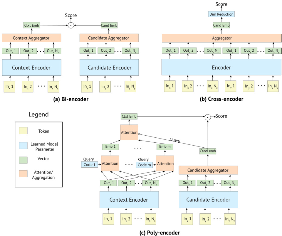
Figure 1: Diagrams of the three model architectures we consider. (a) The Bi-encoder encodes the context and candidate separately, allowing for the caching of candidate representations during inference. (b) The Cross-encoder jointly encodes the context and candidate in a single transformer, yielding richer interactions between context and candidate at the cost of slower computation. (c) The Poly-encoder combines the strengths of the Bi-encoder and Cross-encoder by both allowing for caching of candidate representations and adding a final attention mechanism between global features of the input and a given candidate to give richer interactions before computing a final score.
图 1: 我们考虑的三种模型架构示意图。(a) 双编码器(Bi-encoder)分别编码上下文和候选对象,允许在推理期间缓存候选表示。(b) 交叉编码器(Cross-encoder)在单个Transformer中联合编码上下文和候选对象,以更慢的计算速度为代价实现上下文与候选对象间更丰富的交互。(c) 多编码器(Poly-encoder)结合了双编码器和交叉编码器的优势,既允许缓存候选表示,又在计算最终得分前通过输入全局特征与给定候选对象间的最终注意力机制实现更丰富的交互。
Inference speed Unfortunately, the Cross-encoder does not allow for pre computation of the candidate embeddings. At inference time, every candidate must be concatenated with the input context and must go through a forward pass of the entire model. Thus, this method cannot scale to a large amount of candidates. We discuss this bottleneck further in Section 5.4.
推理速度
遗憾的是,交叉编码器 (Cross-encoder) 无法预先计算候选嵌入。在推理时,每个候选都必须与输入上下文拼接,并通过整个模型的前向传播。因此,该方法无法扩展到大量候选。我们将在第5.4节进一步讨论这一瓶颈。
4.4 Poly-encoder
4.4 多编码器 (Poly-encoder)
The Poly-encoder architecture aims to get the best of both worlds from the Bi- and Cross-encoder. A given candidate label is represented by one vector as in the Bi-encoder, which allows for caching candidates for fast inference time, while the input context is jointly encoded with the candidate, as in the Cross-encoder, allowing the extraction of more information.
Poly-encoder架构旨在结合Bi-encoder和Cross-encoder的优势。给定候选标签通过单个向量表示(如Bi-encoder),可缓存候选以实现快速推理;同时输入上下文与候选联合编码(如Cross-encoder),从而提取更多信息。
The Poly-encoder uses two separate transformers for the context and label like a Bi-encoder, and the candidate is encoded into a single vector $y_{c a n d_{i}}$ . As such, the Poly-encoder method can be implemented using a pre computed cache of encoded responses. However, the input context, which is typically much longer than a candidate, is represented with $m$ vectors $(y_{c t x t}^{1}...y_{c t x t}^{m^{\star}})$ instead of just one as in the Bi-encoder, where $m$ will influence the inference speed. To obtain these $m$ global features that represent the input, we learn $m$ context codes $(c_{1},...,c_{m})$ , where $c_{i}$ extracts representation $y_{c t x t}^{i}$ by attending over all the outputs of the previous layer. That is, we obtain $y_{c t x t}^{i}$ using:
Poly-encoder与Bi-encoder类似,使用两个独立的Transformer分别处理上下文和标签,并将候选编码为单一向量$y_{cand_{i}}$。因此,Poly-encoder方法可通过预计算的编码响应缓存实现。然而,输入上下文(通常比候选文本长得多)会表示为$m$个向量$(y_{ctxt}^{1}...y_{ctxt}^{m^{\star}})$,而非Bi-encoder中的单一向量,其中$m$会影响推理速度。为获取代表输入的$m$个全局特征,我们学习$m$个上下文编码$(c_{1},...,c_{m})$,其中$c_{i}$通过关注前一层所有输出来提取表征$y_{ctxt}^{i}$。具体计算公式如下:
$$
y_{c t x t}^{i}=\sum_{j}w_{j}^{c_{i}}h_{j}\qquad\mathrm{where}\qquad(w_{1}^{c_{i}},..,w_{N}^{c_{i}})=\operatorname{softmax}(c_{i}\cdot h_{1},..,c_{i}\cdot h_{N})
$$
$$
y_{c t x t}^{i}=\sum_{j}w_{j}^{c_{i}}h_{j}\qquad\mathrm{where}\qquad(w_{1}^{c_{i}},..,w_{N}^{c_{i}})=\operatorname{softmax}(c_{i}\cdot h_{1},..,c_{i}\cdot h_{N})
$$
The $m$ context codes are randomly initialized, and learnt during finetuning.
这 $m$ 个上下文编码(token)在微调阶段随机初始化并学习得到。
Finally, given our $m$ global context features, we attend over them using $y_{c a n d_{i}}$ as the query:
最后,给定我们的 $m$ 个全局上下文特征,我们使用 $y_{c a n d_{i}}$ 作为查询对其进行注意力计算:
$$
y_{c t x t}=\sum_{i}w_{i}y_{c t x t}^{i}\qquad\mathrm{where}\qquad(w_{1},..,w_{m})=\operatorname{softmax}(y_{c a n d_{i}}\cdot y_{c t x t}^{1},..,y_{c a n d_{i}}\cdot y_{c t x t}^{m})
$$
$$
y_{c t x t}=\sum_{i}w_{i}y_{c t x t}^{i}\qquad\mathrm{where}\qquad(w_{1},..,w_{m})=\operatorname{softmax}(y_{c a n d_{i}}\cdot y_{c t x t}^{1},..,y_{c a n d_{i}}\cdot y_{c t x t}^{m})
$$
The final score for that candidate label is then $y_{c t x t}\cdot y_{c a n d_{i}}$ as in a Bi-encoder. As $m<N$ , where $N$ is the number of tokens, and the context-candidate attention is only performed at the top layer, this is far faster than the Cross-encoder’s full self-attention.
该候选标签的最终得分即为 $y_{c t x t}\cdot y_{c a n d_{i}}$ ,与双编码器 (Bi-encoder) 的计算方式相同。由于 $m<N$ (其中 $N$ 表示 token 数量),且上下文-候选注意力仅在最顶层执行,因此其速度远快于交叉编码器 (Cross-encoder) 的完全自注意力机制。
5 Experiments
5 实验
We perform a variety of experiments to test our model architectures and training strategies over four tasks. For metrics, we measure Recall $\ @k$ where each test example has $C$ possible candidates to select from, abbreviated to $\mathrm{R}@k/C$ , as well as mean reciprocal rank (MRR).
我们通过四项任务进行了多种实验,以测试模型架构和训练策略。在评估指标方面,我们采用召回率 $\ @k$ (每个测试样本从 $C$ 个候选答案中选择,缩写为 $\mathrm{R}@k/C$ )以及平均倒数排名 (MRR) 进行衡量。
5.1 Bi-encoders and Cross-encoders
5.1 双编码器与交叉编码器
We first investigate fine-tuning the Bi- and Cross-encoder architectures initialized with the weights provided by Devlin et al. (2019), studying the choice of other hyper parameters (we explore our own pre-training schemes in section 5.3). In the case of the Bi-encoder, we can use a large number of negatives by considering the other batch elements as negative training samples, avoiding re computation of their embeddings. On 8 Nvidia Volta v100 GPUs and using half-precision operations (i.e. float16 operations), we can reach batches of 512 elements on ConvAI2. Table 2 shows that in this setting, we obtain higher performance with a larger batch size, i.e. more negatives, where 511 negatives yields the best results. For the other tasks, we keep the batch size at 256, as the longer sequences in those datasets uses more memory. The Cross-encoder is more computationally intensive, as the embeddings for the (context, candidate) pair must be recomputed each time. We thus limit its batch size to 16 and provide negatives random samples from the training set. For DSTC7 and Ubuntu V2, we choose 15 such negatives; For ConvAI2, the dataset provides 19 negatives.
我们首先研究了基于Devlin等人(2019) 提供的权重初始化的双向编码器 (Bi-encoder) 和交叉编码器 (Cross-encoder) 架构的微调,并探讨了其他超参数的选择 (我们在5.3节中探索了自己的预训练方案)。对于双向编码器,我们可以通过将批次中的其他元素视为负样本来使用大量负样本,从而避免重新计算其嵌入向量。在8块Nvidia Volta v100 GPU上使用半精度运算 (即float16运算) 时,我们能在ConvAI2数据集上实现512个元素的批次处理。表2显示,在该设置下,更大的批次规模 (即更多负样本) 能带来更高的性能,其中511个负样本取得了最佳效果。对于其他任务,我们将批次规模保持在256,因为这些数据集中较长的序列会占用更多内存。交叉编码器的计算强度更高,因为每次都必须重新计算 (上下文,候选) 对的嵌入向量。因此我们将其批次规模限制为16,并从训练集中随机抽取负样本。对于DSTC7和Ubuntu V2任务,我们选择15个负样本;对于ConvAI2,数据集本身提供了19个负样本。
| Negatives | 31 | 63 | 127 | 255 | 511 |
| R@ 1/20 | 81.0 | 81.7 | 82.3 | 83.0 | 83.3 |
| Negatives | 31 | 63 | 127 | 255 | 511 |
|---|---|---|---|---|---|
| R@ 1/20 | 81.0 | 81.7 | 82.3 | 83.0 | 83.3 |
Table 2: Validation performance on ConvAI2 after fine-tuning a Bi-encoder pre-trained with BERT, averaged over 5 runs. The batch size is the number of training negatives $^{\mathrm{ + }1}$ as we use the other elements of the batch as negatives during training.
表 2: 基于BERT预训练的双编码器在ConvAI2数据集上的微调验证性能(5次运行平均值)。批次大小为训练负样本数$^{\mathrm{ + }1}$(训练时使用批次内其他元素作为负样本)。
The above results are reported with Bi-encoder aggregation based on the first output. Choosing the average over all outputs instead is very similar but slightly worse (83.1, averaged over 5 runs). We also tried to add further non-linear i ties instead of the inner product of the two representations, but could not obtain improved results over the simpler architecture (results not shown).
上述结果基于首个输出的双编码器聚合报告。若选择对所有输出取平均值,结果非常相似但略差(83.1,5次运行平均值)。我们还尝试添加更多非线性关系替代两种表征的内积运算,但未能获得比简单架构更好的效果(结果未展示)。
We tried two optimizers: Adam (Kingma & Ba, 2015) with weight decay of 0.01 (as recommended by (Devlin et al., 2019)) and Adamax (Kingma & Ba, 2015) without weight decay; based on validation set performance, we choose to fine-tune with Adam when using the BERT weights. The learning rate is initialized to 5e-5 with a warmup of 100 iterations for Bi- and Poly-encoders, and 1000 iterations for the Cross-encoder. The learning rate decays by a factor of 0.4 upon plateau of the loss evaluated on the valid set every half epoch. In Table 3 we show validation performance when fine-tuning various layers of the weights provided by (Devlin et al., 2019), using Adam with decay optimizer. Fine-tuning the entire network is important, with the exception of the word embeddings.
我们尝试了两种优化器:带权重衰减(0.01,遵循 (Devlin et al., 2019) 建议)的 Adam (Kingma & Ba, 2015) 和不带权重衰减的 Adamax (Kingma & Ba, 2015)。根据验证集表现,在使用 BERT 权重时选择 Adam 进行微调。学习率初始设为 5e-5,Bi-encoder 和 Poly-encoder 采用 100 次迭代预热,Cross-encoder 采用 1000 次迭代。当验证集损失每半轮停滞时,学习率以 0.4 倍率衰减。表 3 展示了使用带衰减的 Adam 优化器微调 (Devlin et al., 2019) 提供的各层权重时的验证性能。除词嵌入层外,微调整个网络至关重要。
With the setups described above, we fine-tune the Bi- and Cross-encoders on the datasets, and report the results in Table 4. On the first three tasks, our Bi-encoders and Cross-encoders outperform the best existing approaches in the literature when we fine-tune from BERT weights. E.g., the Biencoder reaches $81.7%$ $\mathbf{R}\ @1$ on ConvAI2 and $66.8%$ $\mathbf{R}\ @1$ on DSTC7, while the Cross-encoder achieves higher scores of $84.8%$ $\mathbf{R}\ @1$ on ConvAI2 and $67.4%$ $\mathbf{R}\ @1$ on DSTC7. Overall, Crossencoders outperform all previous approaches on the three dialogue tasks, including our Bi-encoders (as expected). We do not report fine-tuning of BERT for Wikipedia IR as we cannot guarantee the test set is not part of the pre-training for that dataset. In addition, Cross-encoders are also too slow to evaluate on the evaluation setup of that task, which has 10k candidates.
基于上述设置,我们在数据集上对双向编码器(Bi-encoder)和交叉编码器(Cross-encoder)进行微调,结果如 表 4 所示。在前三项任务中,当从BERT权重微调时,我们的双向编码器和交叉编码器表现优于文献中的现有最佳方法。例如,双向编码器在ConvAI2上达到 $81.7%$ $\mathbf{R}\ @1$ ,在DSTC7上达到 $66.8%$ $\mathbf{R}\ @1$ ,而交叉编码器在ConvAI2上取得更高的 $84.8%$ $\mathbf{R}\ @1$ ,在DSTC7上达到 $67.4%$ $\mathbf{R}\ @1$ 。总体而言,交叉编码器在三项对话任务中超越了所有先前方法(包括我们的双向编码器,这符合预期)。由于无法保证测试集未包含在该数据集的预训练中,我们未报告BERT在维基百科IR任务上的微调结果。此外,交叉编码器在该任务的评估设置(包含1万个候选)中运行速度过慢,难以进行评估。
Table 3: Validation performance $(\mathtt{R@1/20})$ on ConvAI2 using pre-trained weights of BERT-base with different parameters fine-tuned. Average over 5 runs (Bi-encoders) or 3 runs (Cross-encoders).
| Fine-tuned parameters | Bi-encoder | Cross-encoder |
| Toplayer Top 4 layers All but Embeddings | 74.2 | 80.6 |
| 82.0 | 86.3 | |
| 83.3 83.0 | 87.3 86.6 |
表 3: 在ConvAI2上使用不同微调参数的BERT-base预训练权重的验证性能 $(\mathtt{R@1/20})$ 。Bi-encoder为5次运行的平均值,Cross-encoder为3次运行的平均值。
| 微调参数 | Bi-encoder | Cross-encoder |
|---|---|---|
| Toplayer | 74.2 | 80.6 |
| Top 4 layers | 82.0 | 86.3 |
| All but Embeddings | 83.3 83.0 | 87.3 86.6 |
Table 4: Test performance of Bi-, Poly- and Cross-encoders on our selected tasks.
| Dataset | ConvA12 | DSTC 7 | Ubuntu v2 | Wikipedia IR | ||
| split | test | test | test | test | ||
| metric | R@1/20 | R@1/100 | MRR | R@1/10 | MRR | R@1/10001 |
| (Wolf et al., 2019) | 80.7 | |||||
| (Gu et al., 2018) | 60.8 | 69.1 | 二 | 二 | 二 | |
| (Chen&Wang,2019) | - | 64.5 | 73.5 | 二 | ||
| (Yoon et al., 2018) | 二 | 65.2 | 二 | |||
| (Dong&Huang,2018) | 75.9 | 84.8 | ||||
| (Wu et al., 2018) | - | - | 56.8 | |||
| pre-trained BERT weights from (Devlin et al., 2019) - Toronto Books + Wikipedia | ||||||
| Bi-encoder | 81.7 ± 0.2 | 66.8 ± 0.7 | 74.6 ± 0.5 | 80.6 ± 0.4 | 88.0 ± 0.3 | |
| Poly-encoder 16 | 83.2± 0.1 | 67.8 ± 0.3 | 75.1 ± 0.2 | 81.2±0.2 | 88.3 ± 0.1 | 二 |
| Poly-encoder 64 | 83.7 ± 0.2 | 67.0 ± 0.9 | 74.7 ± 0.6 | 81.3 ± 0.2 | 88.4 ± 0.1 | |
| Poly-encoder 360 | 83.7± 0.2 | 68.9 ± 0.4 | 76.2 ± 0.2 | 80.9 ± 0.0 | 88.1 ± 0.1 | 二 |
| Cross-encoder | 84.8 ± 0.3 | 67.4 ± 0.7 | 75.6 ± 0.4 | 82.8 ± 0.3 | 89.4 ± 0.2 | 二 |
| Our pre-training on TorontoBooks +Wikipedia | ||||||
| Bi-encoder | 82.0 ± 0.1 | 64.5 ± 0.5 | 72.6 ± 0.4 | 80.8 ± 0.5 | 88.2 ± 0.4 | 二 |
| Poly-encoder 16 | 82.7 ± 0.1 | 65.3 ± 0.9 | 73.2 ± 0.7 | 83.4 ± 0.2 | 89.9 ± 0.1 | |
| Poly-encoder 64 | 83.3 ± 0.1 | 65.8 ± 0.7 | 73.5± 0.5 | 83.4 ± 0.1 | 89.9 ± 0.0 | |
| Poly-encoder 360 | 83.8 ± 0.1 | 65.8 ± 0.7 | 73.6± 0.6 | 83.7 ± 0.0 | 90.1 ± 0.0 | |
| Cross-encoder | 84.9 ± 0.3 | 65.3 ± 1.0 | 73.8 ± 0.6 | 83.1 ± 0.7 | 89.7 ± 0.5 | |
| Ourpre-trainingonReddit | ||||||
| Bi-encoder | 84.8 ± 0.1 | 70.9 ± 0.5 | 78.1 ± 0.3 | 83.6 ± 0.7 | 90.1 ± 0.4 | 71.0 |
| Poly-encoder 16 | 86.3 ± 0.3 | 71.6 ± 0.6 | 78.4 ± 0.4 | 86.0 ± 0.1 | 91.5 ± 0.1 | 71.5 |
| Poly-encoder 64 | 86.5 ± 0.2 | 71.2 ± 0.8 | 78.2± 0.7 | 85.9 ± 0.1 | 91.5 ± 0.1 | 71.3 |
| Poly-encoder 360 | 86.8 ± 0.1 | 71.4 ± 1.0 | 78.3 ± 0.7 | 85.9 ± 0.1 | 91.5 ± 0.0 | 71.8 |
| Cross-encoder | 87.9 ± 0.2 | 71.7 ± 0.3 | 79.0 ± 0.2 | 86.5 ± 0.1 | 91.9 ± 0.0 | 二 |
表 4: 双编码器、多编码器和交叉编码器在选定任务上的测试性能
| 数据集 | ConvA12 | DSTC 7 | Ubuntu v2 | Wikipedia IR |
|---|---|---|---|---|
| 分割 | test | test | test | test |
| 指标 | R@1/20 | R@1/100 MRR | R@1/10 MRR | R@1/10001 |
| (Wolf et al., 2019) | 80.7 | |||
| (Gu et al., 2018) | 60.8 69.1 | 二 二 | 二 | |
| (Chen&Wang,2019) | - | 64.5 73.5 | 二 | |
| (Yoon et al., 2018) | 二 | 65.2 | 二 | |
| (Dong&Huang,2018) | 75.9 84.8 | |||
| (Wu et al., 2018) | - | - | 56.8 | |
| 预训练BERT权重来自 (Devlin et al., 2019) - Toronto Books + Wikipedia | ||||
| 双编码器 | 81.7 ± 0.2 | 66.8 ± 0.7 74.6 ± 0.5 | 80.6 ± 0.4 88.0 ± 0.3 | |
| 多编码器16 | 83.2 ± 0.1 | 67.8 ± 0.3 75.1 ± 0.2 | 81.2 ± 0.2 88.3 ± 0.1 | 二 |
| 多编码器64 | 83.7 ± 0.2 | 67.0 ± 0.9 74.7 ± 0.6 | 81.3 ± 0.2 88.4 ± 0.1 | |
| 多编码器360 | 83.7 ± 0.2 | 68.9 ± 0.4 76.2 ± 0.2 | 80.9 ± 0.0 88.1 ± 0.1 | 二 |
| 交叉编码器 | 84.8 ± 0.3 | 67.4 ± 0.7 75.6 ± 0.4 | 82.8 ± 0.3 89.4 ± 0.2 | 二 |
| 我们在TorontoBooks + Wikipedia上的预训练 | ||||
| 双编码器 | 82.0 ± 0.1 | 64.5 ± 0.5 72.6 ± 0.4 | 80.8 ± 0.5 88.2 ± 0.4 | 二 |
| 多编码器16 | 82.7 ± 0.1 | 65.3 ± 0.9 73.2 ± 0.7 | 83.4 ± 0.2 89.9 ± 0.1 | |
| 多编码器64 | 83.3 ± 0.1 | 65.8 ± 0.7 73.5 ± 0.5 | 83.4 ± 0.1 89.9 ± 0.0 | |
| 多编码器360 | 83.8 ± 0.1 | 65.8 ± 0.7 73.6 ± 0.6 | 83.7 ± 0.0 90.1 ± 0.0 | |
| 交叉编码器 | 84.9 ± 0.3 | 65.3 ± 1.0 73.8 ± 0.6 | 83.1 ± 0.7 89.7 ± 0.5 | |
| 我们在Reddit上的预训练 | ||||
| 双编码器 | 84.8 ± 0.1 | 70.9 ± 0.5 78.1 ± 0.3 | 83.6 ± 0.7 90.1 ± 0.4 | 71.0 |
| 多编码器16 | 86.3 ± 0.3 | 71.6 ± 0.6 78.4 ± 0.4 | 86.0 ± 0.1 91.5 ± 0.1 | 71.5 |
| 多编码器64 | 86.5 ± 0.2 | 71.2 ± 0.8 78.2 ± 0.7 | 85.9 ± 0.1 91.5 ± 0.1 | 71.3 |
| 多编码器360 | 86.8 ± 0.1 | 71.4 ± 1.0 78.3 ± 0.7 | 85.9 ± 0.1 91.5 ± 0.0 | 71.8 |
| 交叉编码器 | 87.9 ± 0.2 | 71.7 ± 0.3 79.0 ± 0.2 | 86.5 ± 0.1 91.9 ± 0.0 | 二 |
5.2 Poly-encoders
5.2 多编码器 (Poly-encoders)
We train the Poly-encoder using the same batch sizes and optimizer choices as in the Bi-encoder experiments. Results are reported in Table 4 for various values of $m$ context vectors.
我们使用与双编码器实验相同的批次大小和优化器选择来训练多编码器。表4报告了不同上下文向量$m$值的结果。
The Poly-encoder outperforms the Bi-encoder on all the tasks, with more codes generally yielding larger improvements. Our recommendation is thus to use as large a code size as compute time allows (see Sec. 5.4). On DSTC7, the Poly-encoder architecture with BERT pre training reaches $68.9%$ R1 with 360 intermediate context codes; this actually outperforms the Cross-encoder result $(67.4%)$ and is noticeably better than our Bi-encoder result $(66.8%)$ . Similar conclusions are found on Ubuntu V2 and ConvAI2, although in the latter Cross-encoders give slightly better results.
Poly-encoder在所有任务上的表现均优于Bi-encoder,且通常代码数量越多改进幅度越大。因此我们建议在算力允许范围内尽可能使用更大的代码规模(参见第5.4节)。在DSTC7数据集上,采用BERT预训练的Poly-encoder架构通过360个中间上下文代码实现了68.9%的R1值,这一结果不仅超越了Cross-encoder的67.4%,也明显优于我们Bi-encoder实现的66.8%。在Ubuntu V2和ConvAI2数据集上也得出了相似结论,不过在ConvAI2上Cross-encoder的表现略胜一筹。
We note that since reporting our results, the authors of Li et al. (2019) have conducted a human evaluation study on ConvAI2, in which our Poly-encoder architecture outperformed all other models compared against, both generative and retrieval based, including the winners of the competition.
我们注意到,在报告我们的结果后,Li等人 (2019) 对ConvAI2进行了人工评估研究,其中我们的Poly-encoder架构优于所有其他对比模型,包括生成式和基于检索的模型,甚至超过了比赛获胜者。
| Scoring time (ms) | ||||
| CPU | GPU | |||
| Candidates | 1k | 100k | 1k | 100k |
| Bi-encoder | 115 | 160 | 19 | 22 |
| Poly-encoder 16 | 122 | 678 | 18 | 38 |
| Poly-encoder 64 | 126 | 692 | 23 | 46 |
| Poly-encoder 360 | 160 | 837 | 57 | 88 |
| Cross-encoder | 21.7k | 2.2M* | 2.6k | 266k* |
| 评分时间 (ms) | |||
|---|---|---|---|
| CPU | GPU | ||
| 候选数量 | 1k | 100k | 1k |
| 双编码器 (Bi-encoder) | 115 | 160 | 19 |
| 多编码器 16 (Poly-encoder 16) | 122 | 678 | 18 |
| 多编码器 64 (Poly-encoder 64) | 126 | 692 | 23 |
| 多编码器 360 (Poly-encoder 360) | 160 | 837 | 57 |
| 交叉编码器 (Cross-encoder) | 21.7k | 2.2M* | 2.6k |
Table 5: Average time in milliseconds to predict the next dialogue utterance from $C$ possible candidates on ConvAI2. * are inferred.
表 5: 在ConvAI2数据集上从 $C$ 个候选对话语句中预测下一句的平均时间(单位:毫秒)。标*号为推断值。
5.3 Domain-specific Pre-training
5.3 领域特定预训练
We fine-tune our Reddit-pre-trained transformer on all four tasks; we additionally fine-tune a transformer that was pre-trained on the same datasets as BERT, specifically Toronto Books $^+$ Wikipedia. When using our pre-trained weights, we use the Adamax optimizer and optimize all the layers of the transformer including the embeddings. As we do not use weight decay, the weights of the final layer are much larger than those in the final layer of BERT; to avoid saturation of the attention layer in the Poly-encoder, we re-scaled the last linear layer so that the standard deviation of its output matched that of BERT, which we found necessary to achieve good results. We report results of fine-tuning with our pre-trained weights in Table 4. We show that pre-training on Reddit gives further state-ofthe-art performance over our previous results with BERT, a finding that we see for all three dialogue tasks, and all three architectures.
我们在所有四项任务上对经过Reddit预训练的Transformer进行了微调;此外,我们还微调了一个与BERT相同数据集(多伦多图书语料$^+$维基百科)预训练的Transformer。使用预训练权重时,我们采用Adamax优化器,并优化Transformer的所有层(包括嵌入层)。由于未使用权重衰减,最终层的权重远大于BERT的对应层;为避免Poly-encoder中注意力层饱和,我们重新调整了末层线性层的输出标准差,使其与BERT保持一致——这一操作对取得良好结果至关重要。表4展示了采用预训练权重的微调结果:Reddit预训练模型在三个对话任务和三种架构中均超越了此前基于BERT的最佳性能。
The results obtained with fine-tuning on our own transformers pre-trained on Toronto Books $^+$ Wikipedia are very similar to those obtained with the original BERT weights, indicating that the choice of dataset used to pre-train the models impacts the final results, not some other detail in our training. Indeed, as the two settings pre-train with datasets of similar size, we can conclude that choosing a pre-training task (e.g. dialogue data) that is similar to the downstream tasks of interest (e.g. dialogue) is a likely explanation for these performance gains, in line with previous results showing multi-tasking with similar tasks is more useful than with dissimilar ones (Caruana, 1997).
在我们使用多伦多书籍$^+$维基百科数据预训练的Transformer模型上进行微调得到的结果,与使用原始BERT权重获得的结果非常相似。这表明影响最终结果的是模型预训练所用数据集的选择,而非我们训练过程中的其他细节。事实上,由于两种设置使用的预训练数据集规模相近,我们可以得出结论:选择与下游目标任务(如对话)相似的预训练任务(如对话数据)是性能提升的主要原因。这一发现与Caruana (1997) 先前的研究结果一致,即相似任务的多任务学习比不相关任务更具优势。
5.4 Inference Speed
5.4 推理速度
An important motivation for the Poly-encoder architecture is to achieve better results than the Biencoder while also performing at a reasonable speed. Though the Cross-encoder generally yields strong results, it is prohibitively slow. We perform speed experiments to determine the trade-off of improved performance from the Poly-encoder. Specifically, we predict the next utterance for 100 dialogue examples in the ConvAI2 validation set, where the model scores $C$ candidates (in this case, chosen from the training set). We perform these experiments on both CPU-only and GPU setups. CPU computations were run on an 80 core Intel Xeon processor CPU E5-2698. GPU computations were run on a single Nvidia Quadro GP100 using cuda 10.0 and cudnn 7.4.
Poly-encoder架构的一个重要动机是在保持合理速度的同时,取得比Biencoder更好的结果。尽管Cross-encoder通常能产生强劲的表现,但其速度慢到难以实用。我们通过速度实验来衡量Poly-encoder性能提升所付出的代价。具体而言,我们在ConvAI2验证集的100个对话样本上预测下一句话,模型需对$C$个候选语句(此处选自训练集)进行评分。实验分别在纯CPU和GPU环境下进行:CPU测试采用80核Intel Xeon E5-2698处理器,GPU测试使用单块Nvidia Quadro GP100(搭配cuda 10.0和cudnn 7.4)。
We show the average time per example for each architecture in Table 5. The difference in timing between the Bi-encoder and the Poly-encoder architectures is rather minimal when there are only 1000 candidates for the model to consider. The difference is more pronounced when considering 100k candidates, a more realistic setup, as we see a $5{\cdot}6\mathrm{x}$ slowdown for the Poly-encoder variants. Nevertheless, both models are still tractable. The Cross-encoder, however, is 2 orders of magnitude slower than the Bi-encoder and Poly-encoder, rendering it intractable for real-time inference, e.g. when interacting with a dialogue agent, or retrieving from a large set of documents. Thus, Polyencoders, given their desirable performance and speed trade-off, are the preferred method.
我们在表5中展示了每种架构处理每个样本的平均耗时。当模型只需考虑1000个候选时,双编码器(Bi-encoder)与多编码器(Poly-encoder)架构的时间差异相当微小。但在更贴近实际的10万候选场景下,多编码器变体会出现$5{\cdot}6\mathrm{x}$的显著降速。不过这两种模型仍具实用性。相比之下,交叉编码器(Cross-encoder)比双编码器和多编码器慢两个数量级,使其无法应用于实时推理场景(例如与对话智能体交互或海量文档检索)。因此,多编码器凭借其优异的性能与速度平衡成为首选方案。
We additionally report training times in the Appendix, Table 6. Poly-encoders also have the benefit of being $3{-}4\mathbf{X}$ faster to train than Cross-encoders (and are similar in training time to Bi-encoders).
我们还在附录的表6中报告了训练时间。Poly-encoder的另一优势是训练速度比Cross-encoder快$3{-}4\mathbf{X}$倍 (训练时间与Bi-encoder相近)。
6 Conclusion
6 结论
In this paper we present new architectures and pre-training strategies for deep bidirectional transformers in candidate selection tasks. We introduced the Poly-encoder method, which provides a mechanism for attending over the context using the label candidate, while maintaining the ability to precompute each candidate’s representation, which allows for fast real-time inference in a production setup, giving an improved trade off between accuracy and speed. We provided an experimental analysis of those trade-offs for Bi-, Poly- and Cross-encoders, showing that Poly-encoders are more accurate than Bi-encoders, while being far faster than Cross-encoders, which are impractical for real-time use. In terms of training these architectures, we showed that pre-training strategies more closely related to the downstream task bring strong improvements. In particular, pre-training from scratch on Reddit allows us to outperform the results we obtain with BERT, a result that holds for all three model architectures and all three dialogue datasets we tried. However, the methods introduced in this work are not specific to dialogue, and can be used for any task where one is scoring a set of candidates, which we showed for an information retrieval task as well.
本文针对候选选择任务提出了深度双向Transformer的新架构与预训练策略。我们引入的Poly-encoder方法能够利用标签候选对象对上下文进行注意力计算,同时保留预计算每个候选表征的能力,从而在生产环境中实现快速实时推理,在准确性与速度之间取得更优平衡。我们通过实验对比分析了双向编码器(Bi-encoder)、多元编码器(Poly-encoder)和交叉编码器(Cross-encoder)的性能权衡,结果表明:Poly-encoder比Bi-encoder更精准,同时比无法实时应用的Cross-encoder快得多。在训练策略方面,我们发现与下游任务关联更紧密的预训练方法能带来显著提升。特别是在Reddit数据上从头预训练的效果优于BERT基准,这一结论在我们尝试的所有三种模型架构和三个对话数据集上都成立。值得注意的是,本文方法不仅适用于对话场景,还可应用于任何需要对候选集合进行评分的任务,我们在信息检索任务中也验证了其有效性。
References
参考文献
Jianxiong Dong and Jim Huang. Enhance word representation for out-of-vocabulary on ubuntu dialogue corpus. CoRR, abs/1802.02614, 2018. URL http://arxiv.org/abs/1802.02614.
Jianxiong Dong 和 Jim Huang. 针对 Ubuntu 对话语料库中未登录词的词表示增强. CoRR, abs/1802.02614, 2018. URL http://arxiv.org/abs/1802.02614.
A Training Time
训练时间
We report the training time on 8 GPU Volta 100 for the 3 datasets considered and for 4 types of models in Table 6.
我们在表6中报告了8块Volta 100 GPU上针对3个数据集和4种模型类型的训练时间。
Table 6: Training time in hours.
| Dataset | ConvAI2 | DSTC7 | UbuntuV2 |
| Bi-encoder | 2.0 | 4.9 | 7.9 |
| Poly-encoder 16 | 2.7 | 5.5 | 8.0 |
| Poly-encoder 64 | 2.8 | 5.7 | 8.0 |
| Cross-encoder64 | 9.4 | 13.5 | 39.9 |
表 6: 训练时间(单位:小时)。
| Dataset | ConvAI2 | DSTC7 | UbuntuV2 |
|---|---|---|---|
| Bi-encoder | 2.0 | 4.9 | 7.9 |
| Poly-encoder 16 | 2.7 | 5.5 | 8.0 |
| Poly-encoder 64 | 2.8 | 5.7 | 8.0 |
| Cross-encoder64 | 9.4 | 13.5 | 39.9 |
B Reduction layer in Bi-encoder
B 双编码器中的降维层
We provide in Table 7 the results obtained for different types of reductions on top of the Bi-encoder. Specifically we compare the Recall $@$ 1/20 on the ConvAI2 validation set when taking the first output of BERT, the average of the first 16 outputs, the average of the first 64 outputs and all of them except the first one ([S]).
我们在表7中提供了在Bi-encoder基础上应用不同类型降维所获得的结果。具体而言,我们比较了在ConvAI2验证集上的Recall $@$ 1/20指标,分别采用以下处理方式:BERT的第一个输出、前16个输出的平均值、前64个输出的平均值,以及除第一个([S])之外所有输出的平均值。
| Setup | ConvA12validRecall@1/20 |
| Firstoutput | 83.3 |
| Avgfirst16outputs | 82.9 |
| Avgfirst 64 outputs | 82.7 |
| Avg all outputs | 83.1 |
| 设置 | ConvA12validRecall@1/20 |
|---|---|
| 首次输出 | 83.3 |
| 前16次输出平均值 | 82.9 |
| 前64次输出平均值 | 82.7 |
| 全部输出平均值 | 83.1 |
Table 7: Bi-encoder results on the ConvAI2 valid set for different choices of function $r e d(\cdot)$ .
表 7: 不同 $red(\cdot)$ 函数选择在 ConvAI2 验证集上的双编码器结果
C Alternative Choices for Context Vectors
C 上下文向量的替代选择
We considered a few other ways to derive the context vectors $(y_{c t x t}^{1},...,y_{c t x t}^{m})$ of the Poly-encoder from the output $(h_{c t x t}^{1},...,h_{c t x t}^{N})$ of the underlying transformer:
我们考虑了其他几种从底层Transformer的输出$(h_{c t x t}^{1},...,h_{c t x t}^{N})$推导Poly-encoder上下文向量$(y_{c t x t}^{1},...,y_{c t x t}^{m})$的方法:
The performance of those four methods is evaluated on the validation set of Convai2 and DSTC7 and reported on Table 8. The first two methods are shown in Figure 2. We additionally provide the inference time for a given number of candidates coming from the Convai2 dataset on Table 9.
这四种方法的性能在Convai2和DSTC7的验证集上进行了评估,结果如 表 8 所示。前两种方法如 图 2 所示。我们还在 表 9 中提供了Convai2数据集给定候选数量的推理时间。
Table 8: Validation and test performance of Poly-encoder variants, with weights initialized from (Devlin et al., 2019). Scores are shown for ConvAI2 and DSTC 7 Track 1. Bold numbers indicate the highest performing variant within that number of codes.
| Dataset | ConvAI2 | DSTC 7 | ||
| split | dev | test | dev | test |
| metric | R@ 1/20 | R@1/20 | R@1/100 | R@1/100 |
| (Wolf et al., 2019) | 82.1 | 80.7 | - | - |
| (Chen & Wang, 2019) | - | - | 57.3 | 64.5 |
| 1 Attention Code | ||||
| Learnt-codes First m outputs Last m outputs | 81.9 ± 0.3 83.2 ± 0.2 82.9 ± 0.1 | 81.0 ± 0.1 81.5 ± 0.1 81.0 ± 0.1 | 56.2 ± 0.1 56.4 ± 0.3 56.1 ± 0.4 | 66.9 ± 0.7 66.8 ± 0.7 67.2 ± 1.1 |
| Last m outputs and hl ctxt 4AttentionCodes | ||||
| Learnt-codes First m outputs Last m outputs | 83.8 ± 0.2 83.4 ± 0.2 82.8 ± 0.2 82.9 ± 0.1 | 82.2 ± 0.5 81.6 ± 0.1 81.3 ± 0.4 81.4 ± 0.2 | 56.5± 0.5 56.9 ± 0.5 56.0 ± 0.5 55.8 ± 0.3 | 66.8 ± 0.7 67.2 ± 1.3 65.8 ± 0.5 66.1 ± 0.8 |
| 16 Attention Codes | ||||
| Learnt-codes First m outputs Last m outputs Last m outputs and ht t.x | 84.4 ± 0.1 85.2 ± 0.1 83.9 ± 0.2 83.8 ± 0.3 | 83.2 ± 0.1 83.9 ± 0.2 82.0 ± 0.4 81.7 ± 0.3 | 57.7 ± 0.2 56.1 ± 1.7 56.1 ± 0.3 56.1 ± 0.3 | 67.8 ± 0.3 66.8 ± 1.1 66.2 ± 0.7 66.6 ± 0.2 |
| 64 Attention Codes Learnt-codes | ||||
| First m outputs Last m outputs Last m outputs and ht ctxt | 84.9 ± 0.1 86.0 ± 0.2 84.9 ± 0.3 85.0 ± 0.2 | 83.7 ± 0.2 84.2 ± 0.2 82.9 ± 0.2 83.2 ± 0.2 | 58.3 ± 0.4 57.7 ± 0.6 57.0 ± 0.2 57.3 ± 0.3 | 67.0 ± 0.9 67.1 ± 0.1 66.5 ± 0.5 67.1 ± 0.5 |
| 360 Attention Codes | ||||
| Learnt-codes First m outputs | 85.3 ± 0.3 86.3 ± 0.1 | 83.7 ± 0.2 84.6 ± 0.3 | 57.7 ± 0.3 58.1 ± 0.4 | 68.9 ± 0.4 66.8 ± 0.7 |
| Last m outputs | 86.3 ± 0.1 | 84.7 ± 0.3 | 58.0 ± 0.4 | 68.1 ± 0.5 |
| Last m outputs and hl ctxt | 86.2 ± 0.3 | 84.5 ± 0.4 | 58.3 ± 0.4 | 68.0 ± 0.8 |
表 8: Poly-encoder变体的验证和测试性能,权重初始化自 (Devlin et al., 2019)。展示了ConvAI2和DSTC 7 Track 1的得分。加粗数字表示在该编码数量下性能最高的变体。
| 数据集 | ConvAI2 | DSTC 7 | ||
|---|---|---|---|---|
| 分割 | 开发集 | 测试集 | 开发集 | 测试集 |
| 指标 | R@1/20 | R@1/20 | R@1/100 | R@1/100 |
| (Wolf et al., 2019) | 82.1 | 80.7 | - | - |
| (Chen & Wang, 2019) | - | - | 57.3 | 64.5 |
| 1 Attention Code | ||||
| Learnt-codes First m outputs Last m outputs | 81.9 ± 0.3 83.2 ± 0.2 82.9 ± 0.1 | 81.0 ± 0.1 81.5 ± 0.1 81.0 ± 0.1 | 56.2 ± 0.1 56.4 ± 0.3 56.1 ± 0.4 | 66.9 ± 0.7 66.8 ± 0.7 67.2 ± 1.1 |
| Last m outputs and hl ctxt 4AttentionCodes | ||||
| Learnt-codes First m outputs Last m outputs | 83.8 ± 0.2 83.4 ± 0.2 82.8 ± 0.2 82.9 ± 0.1 | 82.2 ± 0.5 81.6 ± 0.1 81.3 ± 0.4 81.4 ± 0.2 | 56.5± 0.5 56.9 ± 0.5 56.0 ± 0.5 55.8 ± 0.3 | 66.8 ± 0.7 67.2 ± 1.3 65.8 ± 0.5 66.1 ± 0.8 |
| 16 Attention Codes | ||||
| Learnt-codes First m outputs Last m outputs Last m outputs and ht t.x | 84.4 ± 0.1 85.2 ± 0.1 83.9 ± 0.2 83.8 ± 0.3 | 83.2 ± 0.1 83.9 ± 0.2 82.0 ± 0.4 81.7 ± 0.3 | 57.7 ± 0.2 56.1 ± 1.7 56.1 ± 0.3 56.1 ± 0.3 | 67.8 ± 0.3 66.8 ± 1.1 66.2 ± 0.7 66.6 ± 0.2 |
| 64 Attention Codes Learnt-codes | ||||
| First m outputs Last m outputs Last m outputs and ht ctxt | 84.9 ± 0.1 86.0 ± 0.2 84.9 ± 0.3 85.0 ± 0.2 | 83.7 ± 0.2 84.2 ± 0.2 82.9 ± 0.2 83.2 ± 0.2 | 58.3 ± 0.4 57.7 ± 0.6 57.0 ± 0.2 57.3 ± 0.3 | 67.0 ± 0.9 67.1 ± 0.1 66.5 ± 0.5 67.1 ± 0.5 |
| 360 Attention Codes | ||||
| Learnt-codes First m outputs | 85.3 ± 0.3 86.3 ± 0.1 | 83.7 ± 0.2 84.6 ± 0.3 | 57.7 ± 0.3 58.1 ± 0.4 | 68.9 ± 0.4 66.8 ± 0.7 |
| Last m outputs | 86.3 ± 0.1 | 84.7 ± 0.3 | 58.0 ± 0.4 | 68.1 ± 0.5 |
| Last m outputs and hl ctxt | 86.2 ± 0.3 | 84.5 ± 0.4 | 58.3 ± 0.4 | 68.0 ± 0.8 |
Table 9: Average time in milliseconds to predict the next dialogue utterance from $N$ possible candidates. * are inferred.
| Scoring time (ms) | ||||
| CPU | GPU | |||
| Candidates | 1k | 100k | 1k | 100k |
| Bi-encoder | 115 | 160 | 19 | 22 |
| Poly-encoder (First m outputs) 16 | 119 | 551 | 17 | 37 |
| Poly-encoder (First m outputs) 64 | 124 | 570 | 17 | 39 |
| Poly-encoder (First m outputs) 360 | 120 | 619 | 17 | 45 |
| Poly-encoder (Learnt-codes) 16 | 122 | 678 | 18 | 38 |
| Poly-encoder (Learnt-codes) 64 | 126 | 692 | 23 | 46 |
| Poly-encoder (Learnt-codes) 360 | 160 | 837 | 57 | 88 |
| Cross-encoder | 21.7k | 2.2M* | 2.6k | 266k* |
表 9: 从 $N$ 个候选对话语句中预测下一个语句的平均时间(毫秒)。* 表示推断值。
| 候选模型 | CPU(1k) | CPU(100k) | GPU(1k) | GPU(100k) |
|---|---|---|---|---|
| Bi-encoder | 115 | 160 | 19 | 22 |
| Poly-encoder(前m个输出)16 | 119 | 551 | 17 | 37 |
| Poly-encoder(前m个输出)64 | 124 | 570 | 17 | 39 |
| Poly-encoder(前m个输出)360 | 120 | 619 | 17 | 45 |
| Poly-encoder(学习编码)16 | 122 | 678 | 18 | 38 |
| Poly-encoder(学习编码)64 | 126 | 692 | 23 | 46 |
| Poly-encoder(学习编码)360 | 160 | 837 | 57 | 88 |
| Cross-encoder | 21.7k | 2.2M* | 2.6k | 266k* |

Figure 2: (a) The Bi-encoder (b) The Cross-encoder (c) The Poly-encoder with first m vectors. (d) The Poly-encoder with $m$ learnt codes.
图 2: (a) 双编码器 (Bi-encoder) (b) 交叉编码器 (Cross-encoder) (c) 带前m个向量的多编码器 (Poly-encoder) (d) 带$m$个学习编码的多编码器。
| Dataset | ConvAI2 | DSTC 7 | Ubuntu v2 | |||||||
| split | dev | test | dev | test | dev | test | ||||
| metric | R@1/20 | R@1/20 | R@1/100 | R@1/100R@10/100 | MRR | R@1/10 | R@1/10 | R@5/10 | MRR | |
| Hugging Face | 82.1 | 80.7 | ||||||||
| (Wolf et al., 2019) (Chen&Wang,2019) | 57.3 | 64.5 | 90.2 | 73.5 | ||||||
| (Dong&Huang,2018) | 75.9 | 97.3 | 84.8 | |||||||
| pre-trained weights from (Devlin et al., 2019) - Toronto Books + Wikipedia | ||||||||||
| Bi-encoder | 83.3± 0.2 | 81.7± 0.2 | 56.5 ± 0.4 | 66.8 ± 0.7 | 89.0 ± 1.0 | 74.6 ± 0.5 | 80.9 ± 0.6 | 80.6± 0.4 | 98.2± 0.1 | 88.0± 0.3 |
| Poly-encoder (First-m) 16 | 85.2 ± 0.1 | 83.9 ± 0.2 | 56.7 ± 0.2 | 67.0 ± 0.9 | 88.8± 0.3 | 74.6 ± 0.6 | 81.7 ± 0.5 | 81.4 ± 0.6 | 98.2 ± 0.1 | 88.5 ± 0.4 |
| Poly-encoder (Learnt-m) 16 | 84.4 ± 0.1 | 83.2 ± 0.1 | 57.7 ± 0.2 | 67.8 ± 0.3 | 88.6 ± 0.2 | 75.1 ± 0.2 | 81.5 ± 0.1 | 81.2 ± 0.2 | 98.2± 0.0 | 88.3 ± 0.1 |
| Poly-encoder (First-m) 64 | 86.0 ± 0.2 | 84.2 ± 0.2 | 57.1 ± 0.2 | 66.9 ± 0.7 | 89.1 ± 0.2 | 74.7 ± 0.4 | 82.2± 0.6 | 81.9± 0.5 | 98.4 ± 0.0 | 88.8 ± 0.3 |
| Poly-encoder(Learnt-m)64 | 84.9 ± 0.1 | 83.7 ± 0.2 | 58.3 ± 0.4 | 67.0 ± 0.9 | 89.2 ± 0.2 | 74.7 ± 0.6 | 81.8 ± 0.1 | 81.3 ± 0.2 | 98.2 ± 0.1 | 88.4 ± 0.1 |
| Poly-encoder (First-m)360 | 86.3 ± 0.1 | 84.6 ± 0.3 | 57.8 ± 0.5 | 67.0 ± 0.5 | 89.6 ± 0.9 | 75.0 ± 0.6 | 82.7 ± 0.4 | 82.2 ± 0.6 | 98.4 ± 0.1 | 89.0 ± 0.4 |
| Poly-encoder (Learnt-m) 360 | 85.3 ± 0.3 | 83.7 ± 0.2 | 57.7 ± 0.3 | 68.9 ± 0.4 | 89.9 ± 0.5 | 76.2 ± 0.2 | 81.5 ± 0.1 | 80.9 ± 0.1 | 98.1± 0.0 | 88.1 ± 0.1 |
| Cross-encoder | 87.1 ± 0.1 | 84.8 ± 0.3 | 59.4 ± 0.4 | 67.4 ± 0.7 | 90.5± 0.3 | 75.6 ± 0.4 | 83.3 ± 0.4 | 82.8 ± 0.3 | 98.4 ± 0.1 | 89.4 ± 0.2 |
| Our pre-training onTorontoBooks+Wikipedia | ||||||||||
| Bi-encoder | 84.6 ± 0.1 | 82.0 ± 0.1 | 54.9 ± 0.5 | 64.5 ± 0.5 | 88.1 ± 0.2 | 72.6 ± 0.4 | 80.9 ± 0.5 | 80.8± 0.5 | 98.4 ± 0.1 | 88.2 ± 0.4 |
| Poly-encoder (First-m) 16 | 84.1 ± 0.2 | 81.4 ± 0.2 | 53.9 ± 2.7 | 63.3 ± 2.9 | 87.2 ± 1.5 | 71.6 ± 2.4 | 80.8 ± 0.5 | 80.6 ± 0.4 | 98.4 ± 0.1 | 88.1 ± 0.3 |
| Poly-encoder (Learnt-m) 16 | 85.4 ± 0.2 | 82.7 ± 0.1 | 56.0 ± 0.4 | 65.3 ± 0.9 | 88.2± 0.7 | 73.2 ± 0.7 | 84.0 ± 0.1 | 83.4 ± 0.2 | 98.7 ± 0.0 | 89.9 ± 0.1 |
| Poly-encoder (First-m) 64 | 86.1 ± 0.4 | 83.9 ± 0.3 | 55.6 ± 0.9 | 64.3 ± 1.5 | 87.8 ± 0.4 | 72.5 ± 1.0 | 80.9 ± 0.6 | 80.7 ± 0.6 | 98.4 ± 0.0 | 88.2 ± 0.4 |
| Poly-encoder (Learnt-m) 64 | 85.6 ± 0.1 | 83.3 ± 0.1 | 56.2 ± 0.4 | 65.8 ± 0.7 | 88.4 ± 0.3 | 73.5 ± 0.5 | 84.0 ± 0.1 | 83.4 ± 0.1 | 98.7± 0.0 | 89.9 ± 0.0 |
| Poly-encoder (First-m) 360 | 86.6 ± 0.3 | 84.4 ± 0.2 | 57.5 ± 0.4 | 66.5 ± 1.2 | 89.0 ± 0.5 | 74.4 ± 0.7 | 81.3 ± 0.6 | 81.1 ± 0.4 | 98.4± 0.2 | 88.4 ± 0.3 |
| Poly-encoder(Learnt-m)360 | 86.1 ± 0.1 | 83.8 ± 0.1 | 56.5 ± 0.8 | 65.8 ± 0.7 | 88.5 ± 0.6 | 73.6 ± 0.6 | 84.2 ± 0.2 | 83.7 ± 0.0 | 98.7 ± 0.1 | 90.1 ± 0.0 |
| Cross-encoder Our pre-training on Reddit | 87.3 ± 0.5 | 84.9 ± 0.3 | 57.7 ± 0.5 | 65.3 ± 1.0 | 89.7 ± 0.5 | 73.8 ± 0.6 | 83.2 ± 0.8 | 83.1 ± 0.7 | 98.7 ± 0.1 | 89.7 ± 0.5 |
| Bi-encoder | 86.9 ± 0.1 | 84.8 ± 0.1 | 60.1 ± 0.4 | 70.9 ± 0.5 | 90.6 ± 0.3 | 78.1 ± 0.3 | 83.7 ± 0.7 | 83.6 ± 0.7 | 98.8 ± 0.1 | 90.1 ± 0.4 |
| Poly-encoder (First-m) 16 | 89.0 ± 0.1 | 86.4 ± 0.3 | 60.4 ± 0.3 | 70.7 ± 0.7 | 91.0 ± 0.4 | 78.0 ± 0.5 | 84.3 ± 0.3 | 84.3 ± 0.2 | 98.9 ± 0.0 | 90.5 ± 0.1 |
| Poly-encoder(Learnt-m)16 | 88.6 ± 0.3 | 86.3 ± 0.3 | 61.1 ± 0.4 | 71.6 ± 0.6 | 91.3 ± 0.3 | 78.4 ± 0.4 | 86.1 ± 0.1 | 86.0 ± 0.1 | 99.0 ± 0.1 | 91.5 ± 0.1 |
| Poly-encoder (First-m) 64 | 89.5 ± 0.1 | 87.3 ± 0.2 | 61.0 ± 0.4 | 70.9 ± 0.6 | 91.5 ± 0.5 | 78.0 ± 0.3 | 84.0 ± 0.4 | 83.9 ± 0.4 | 98.8 ± 0.0 | 90.3 ± 0.3 |
| Poly-encoder (Learnt-m) 64 | 89.0 ± 0.1 | 86.5 ± 0.2 | 60.9 ± 0.6 | 71.2 ± 0.8 | 91.3 ± 0.4 | 78.2 ± 0.7 | 86.2 ± 0.1 | 85.9 ± 0.1 | 99.1 ± 0.0 | 91.5 ± 0.1 |
| Poly-encoder (First-m) 360 | 10+0:06 | 87.3 ± 0.1 | 61.1 ± 1.9 | 70.9 ± 2.1 | 91.5 ± 0.9 | 77.9 ± 1.6 | 84.8 ± 0.5 | 84.6 ± 0.5 | 98.9 ± 0.1 | 90.7 ± 0.3 |
| Poly-encoder (Learnt-m) 360 | 89.2 ± 0.1 | 86.8 ± 0.1 | 61.2 ± 0.2 | 71.4 ± 1.0 | 91.1 ± 0.3 | 78.3 ± 0.7 | 86.3 ± 0.1 | 85.9 ± 0.1 | 99.1 ± 0.0 | 91.5 ± 0.0 |
| Cross-encoder | 90.3 ± 0.2 | 87.9 ± 0.2 | 63.9 ± 0.3 | 71.7 ± 0.3 | 92.4 ± 0.5 | 79.0 ± 0.2 | 86.7 ± 0.1 | 86.5 ± 0.1 | 99.1 ± 0.0 | 91.9 ± 0.0 |
| 数据集 | ConvAI2 | DSTC 7 | Ubuntu v2 | |||||||
|---|---|---|---|---|---|---|---|---|---|---|
| 划分 | 开发集 | 测试集 | 开发集 | 测试集 | 开发集 | 测试集 | ||||
| 指标 | R@1/20 | R@1/20 | R@1/100 | R@1/100 | R@10/100 | MRR | R@1/10 | R@1/10 | R@5/10 | MRR |
| Hugging Face | 82.1 | 80.7 | ||||||||
| (Wolf et al., 2019) (Chen&Wang,2019) | 57.3 | 64.5 | 90.2 | 73.5 | ||||||
| (Dong&Huang,2018) | 75.9 | 97.3 | 84.8 | |||||||
| 预训练权重来自 (Devlin et al., 2019) - Toronto Books + Wikipedia | ||||||||||
| 双编码器 | 83.3±0.2 | 81.7±0.2 | 56.5±0.4 | 66.8±0.7 | 89.0±1.0 | 74.6±0.5 | 80.9±0.6 | 80.6±0.4 | 98.2±0.1 | 88.0±0.3 |
| 多编码器 (First-m) 16 | 85.2±0.1 | 83.9±0.2 | 56.7±0.2 | 67.0±0.9 | 88.8±0.3 | 74.6±0.6 | 81.7±0.5 | 81.4±0.6 | 98.2±0.1 | 88.5±0.4 |
| 多编码器 (Learnt-m) 16 | 84.4±0.1 | 83.2±0.1 | 57.7±0.2 | 67.8±0.3 | 88.6±0.2 | 75.1±0.2 | 81.5±0.1 | 81.2±0.2 | 98.2±0.0 | 88.3±0.1 |
| 多编码器 (First-m) 64 | 86.0±0.2 | 84.2±0.2 | 57.1±0.2 | 66.9±0.7 | 89.1±0.2 | 74.7±0.4 | 82.2±0.6 | 81.9±0.5 | 98.4±0.0 | 88.8±0.3 |
| 多编码器 (Learnt-m) 64 | 84.9±0.1 | 83.7±0.2 | 58.3±0.4 | 67.0±0.9 | 89.2±0.2 | 74.7±0.6 | 81.8±0.1 | 81.3±0.2 | 98.2±0.1 | 88.4±0.1 |
| 多编码器 (First-m) 360 | 86.3±0.1 | 84.6±0.3 | 57.8±0.5 | 67.0±0.5 | 89.6±0.9 | 75.0±0.6 | 82.7±0.4 | 82.2±0.6 | 98.4±0.1 | 89.0±0.4 |
| 多编码器 (Learnt-m) 360 | 85.3±0.3 | 83.7±0.2 | 57.7±0.3 | 68.9±0.4 | 89.9±0.5 | 76.2±0.2 | 81.5±0.1 | 80.9±0.1 | 98.1±0.0 | 88.1±0.1 |
| 交叉编码器 | 87.1±0.1 | 84.8±0.3 | 59.4±0.4 | 67.4±0.7 | 90.5±0.3 | 75.6±0.4 | 83.3±0.4 | 82.8±0.3 | 98.4±0.1 | 89.4±0.2 |
| 我们在TorontoBooks+Wikipedia上的预训练 | ||||||||||
| 双编码器 | 84.6±0.1 | 82.0±0.1 | 54.9±0.5 | 64.5±0.5 | 88.1±0.2 | 72.6±0.4 | 80.9±0.5 | 80.8±0.5 | 98.4±0.1 | 88.2±0.4 |
| 多编码器 (First-m) 16 | 84.1±0.2 | 81.4±0.2 | 53.9±2.7 | 63.3±2.9 | 87.2±1.5 | 71.6±2.4 | 80.8±0.5 | 80.6±0.4 | 98.4±0.1 | 88.1±0.3 |
| 多编码器 (Learnt-m) 16 | 85.4±0.2 | 82.7±0.1 | 56.0±0.4 | 65.3±0.9 | 88.2±0.7 | 73.2±0.7 | 84.0±0.1 | 83.4±0.2 | 98.7±0.0 | 89.9±0.1 |
| 多编码器 (First-m) 64 | 86.1±0.4 | 83.9±0.3 | 55.6±0.9 | 64.3±1.5 | 87.8±0.4 | 72.5±1.0 | 80.9±0.6 | 80.7±0.6 | 98.4±0.0 | 88.2±0.4 |
| 多编码器 (Learnt-m) 64 | 85.6±0.1 | 83.3±0.1 | 56.2±0.4 | 65.8±0.7 | 88.4±0.3 | 73.5±0.5 | 84.0±0.1 | 83.4±0.1 | 98.7±0.0 | 89.9±0.0 |
| 多编码器 (First-m) 360 | 86.6±0.3 | 84.4±0.2 | 57.5±0.4 | 66.5±1.2 | 89.0±0.5 | 74.4±0.7 | 81.3±0.6 | 81.1±0.4 | 98.4±0.2 | 88.4±0.3 |
| 多编码器 (Learnt-m) 360 | 86.1±0.1 | 83.8±0.1 | 56.5±0.8 | 65.8±0.7 | 88.5±0.6 | 73.6±0.6 | 84.2±0.2 | 83.7±0.0 | 98.7±0.1 | 90.1±0.0 |
| 交叉编码器 我们在Reddit上的预训练 | 87.3±0.5 | 84.9±0.3 | 57.7±0.5 | 65.3±1.0 | 89.7±0.5 | 73.8±0.6 | 83.2±0.8 | 83.1±0.7 | 98.7±0.1 | 89.7±0.5 |
| 双编码器 | 86.9±0.1 | 84.8±0.1 | 60.1±0.4 | 70.9±0.5 | 90.6±0.3 | 78.1±0.3 | 83.7±0.7 | 83.6±0.7 | 98.8±0.1 | 90.1±0.4 |
| 多编码器 (First-m) 16 | 89.0±0.1 | 86.4±0.3 | 60.4±0.3 | 70.7±0.7 | 91.0±0.4 | 78.0±0.5 | 84.3±0.3 | 84.3±0.2 | 98.9±0.0 | 90.5±0.1 |
| 多编码器 (Learnt-m) 16 | 88.6±0.3 | 86.3±0.3 | 61.1±0.4 | 71.6±0.6 | 91.3±0.3 | 78.4±0.4 | 86.1±0.1 | 86.0±0.1 | 99.0±0.1 | 91.5±0.1 |
| 多编码器 (First-m) 64 | 89.5±0.1 | 87.3±0.2 | 61.0±0.4 | 70.9±0.6 | 91.5±0.5 | 78.0±0.3 | 84.0±0.4 | 83.9±0.4 | 98.8±0.0 | 90.3±0.3 |
| 多编码器 (Learnt-m) 64 | 89.0±0.1 | 86.5±0.2 | 60.9±0.6 | 71.2±0.8 | 91.3±0.4 | 78.2±0.7 | 86.2±0.1 | 85.9±0.1 | 99.1±0.0 | 91.5±0.1 |
| 多编码器 (First-m) 360 | 10+0:06 | 87.3±0.1 | 61.1±1.9 | 70.9±2.1 | 91.5±0.9 | 77.9±1.6 | 84.8±0.5 | 84.6±0.5 | 98.9±0.1 | 90.7±0.3 |
| 多编码器 (Learnt-m) 360 | 89.2±0.1 | 86.8±0.1 | 61.2±0.2 | 71.4±1.0 | 91.1±0.3 | 78.3±0.7 | 86.3±0.1 | 85.9±0.1 | 99.1±0.0 | 91.5±0.0 |
| 交叉编码器 | 90.3±0.2 | 87.9±0.2 | 63.9±0.3 | 71.7±0.3 | 92.4±0.5 | 79.0±0.2 | 86.7±0.1 | 86.5±0.1 | 99.1±0.0 | 91.9±0.0 |
Table 10: Validation and test performances of Bi-, Poly- and Cross-encoders. Scores are shown for ConvAI2, DSTC7 Track 1 and Ubuntu v2, and the previous state-of-the-art models in the literature.
表 10: 双向编码器、多向编码器和交叉编码器的验证与测试性能。展示了ConvAI2、DSTC7 Track 1和Ubuntu v2数据集上的得分,以及文献中先前的最先进模型。