Hierarchically-Refined Label Attention Network for Sequence Labeling
层次精细化标签注意力网络在序列标注中的应用
Abstract
摘要
CRF has been used as a powerful model for statistical sequence labeling. For neural sequence labeling, however, BiLSTM-CRF does not always lead to better results compared with BiLSTM-softmax local classification. This can be because the simple Markov label transition model of CRF does not give much information gain over strong neural encoding. For better representing label sequences, we investigate a hierarchically-refined label attention network, which explicitly leverages label embeddings and captures potential long-term label dependency by giving each word incrementally refined label distributions with hierarchical attention. Results on POS tagging, NER and CCG super tagging show that the proposed model not only improves the overall tagging accuracy with similar number of parameters, but also significantly speeds up the training and testing compared to BiLSTM-CRF.
CRF作为一种强大的统计序列标注模型被广泛应用。然而在神经序列标注任务中,与BiLSTM-softmax局部分类相比,BiLSTM-CRF并不总能取得更好的效果。这可能是因为CRF简单的马尔可夫标签转移模型在强大的神经编码基础上未能提供显著的信息增益。为了更好地表征标签序列,我们研究了一种层次化细化的标签注意力网络,该网络通过显式利用标签嵌入(label embeddings),并借助分层注意力机制为每个单词逐步细化标签分布,从而捕捉潜在的长期标签依赖关系。在词性标注(POS tagging)、命名实体识别(NER)和组合范畴语法超标注(CCG super tagging)任务上的实验表明,所提出的模型在参数量相近的情况下不仅提高了整体标注准确率,而且相比BiLSTM-CRF显著加快了训练和测试速度。
1 Introduction
1 引言
Conditional random fields (CRF) (Lafferty et al., 2001) is a state-of-the-art model for statistical sequence labeling (Toutanova et al., 2003; Peng et al., 2004; Ratinov and Roth, 2009). Recently, CRF has been integrated with neural encoders as an output layer to capture label transition patterns (Zhou and Xu, 2015; Ma and Hovy, 2016). This, however, sees mixed results. For example, previous work (Reimers and Gurevych, 2017; Yang et al., 2018) has shown that BiLSTM-softmax gives better accuracies compared to BiLSTMCRF for part-of-speech (POS) tagging. In addition, the state-of-the-art neural Comb in a tory Categorial Grammar (CCG) super tag gers do not use CRF (Xu et al., 2015; Lewis et al., 2016).
条件随机场 (Conditional Random Fields, CRF) (Lafferty et al., 2001) 是统计序列标注任务的前沿模型 (Toutanova et al., 2003; Peng et al., 2004; Ratinov and Roth, 2009)。近年来,CRF 常与神经编码器结合作为输出层来捕捉标签转移模式 (Zhou and Xu, 2015; Ma and Hovy, 2016),但效果参差不齐。例如,已有研究 (Reimers and Gurevych, 2017; Yang et al., 2018) 表明,在词性标注 (Part-of-Speech Tagging) 任务中,BiLSTM-softmax 的准确率优于 BiLSTM-CRF。此外,当前最先进的神经组合范畴语法 (Combinatory Categorial Grammar, CCG) 超标注器也未采用 CRF 结构 (Xu et al., 2015; Lewis et al., 2016)。
One possible reason is that the strong represent ation power of neural sentence encoders such as BiLSTMs allow models to capture implicit long-range label dependencies from input word sequences alone (Ki per wasser and Goldberg, 2016; Dozat and Manning, 2016; Teng and Zhang, 2018), thereby allowing the output layer to make local predictions. In contrast, though explicitly capturing output label dependencies, CRF can be limited by its Markov assumptions, particularly when being used on top of neural encoders. In addition, CRF can be computationally expensive when the number of labels is large, due to the use of Viterbi decoding.
一个可能的原因是,像BiLSTM这样的神经句子编码器具有强大的表征能力,使模型仅从输入词序列就能捕捉隐含的长距离标签依赖关系 (Kiperwasser and Goldberg, 2016; Dozat and Manning, 2016; Teng and Zhang, 2018),从而让输出层能够进行局部预测。相比之下,尽管CRF显式地捕捉了输出标签依赖关系,但其马尔可夫假设可能会带来限制,尤其是在神经编码器之上使用时。此外,由于使用了维特比解码,当标签数量较大时,CRF的计算开销会很高。
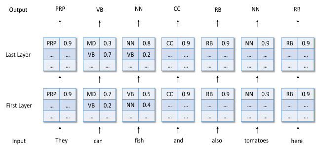
Figure 1: Visualization of hierarchically-refined Label Attention Network for POS tagging. The numbers indicate the label probability distribution for each word.
图 1: 用于词性标注的分层精化标签注意力网络可视化。数字表示每个单词的标签概率分布。
One interesting research question is whether there is neural alternative to CRF for neural sequence labeling, which is both faster and more accurate. To this question, we investigate a neural network model for output label sequences. In particular, we represent each possible label using an embedding vector, and aim to encode sequences of label distributions using a recurrent neural network. One main challenge, however, is that the number of possible label sequences is exponential to the size of input. This makes our task essentially to represent a full-exponential search space without making Markov assumptions.
一个有趣的研究问题是,是否存在比CRF更快且更准确的神经序列标注替代方案。针对这一问题,我们研究了一种用于输出标签序列的神经网络模型。具体而言,我们使用嵌入向量表示每个可能的标签,并旨在通过循环神经网络对标签分布序列进行编码。然而,主要挑战在于可能的标签序列数量与输入规模呈指数级增长。这使得我们的任务本质上是在不做马尔可夫假设的情况下表示一个完全指数级的搜索空间。
We tackle this challenge using a hierarchicallyrefined representation of marginal label distributions. As shown in Figure 1, our model consists of a multi-layer neural network. In each layer, each input words is represented together with its marginal label probabilities, and a sequence neural network is employed to model unbounded dependencies. The marginal distributions space are refined hierarchically bottom-up, where a higher layer learns a more informed label sequence distribution based on information from a lower layer.
我们采用分层细化的边缘标签分布表示来解决这一挑战。如图 1 所示,我们的模型由多层神经网络组成。在每一层中,每个输入词都与其边缘标签概率一起表示,并采用序列神经网络来建模无界依赖关系。边缘分布空间自底向上分层细化,其中更高层基于来自较低层的信息学习更知情的标签序列分布。
For instance, given a sentence “They $\mathrm{\Delta_{1}}$ can2 fish3 $\mathrm{and_{4}}$ $\mathrm{also_{5}}$ tomatoes6 here7”, the label distributions of the words $c a n_{2}$ and in the first layer of Figure 1 have higher probabilities on the tags MD (modal verb) and VB (base form verb), respectively, though not fully confidently. The initial label distributions are then fed as the inputs to the next layer, so that long-range label dependencies can be considered. In the second layer, the network can learn to assign a noun tag to fish3 by taking into account the highly confident tagging information of tomatoes6 (NN), resulting in the pattern .
例如,给定句子 "They $\mathrm{\Delta_{1}}$ can2 fish3 $\mathrm{and_{4}}$ $\mathrm{also_{5}}$ tomatoes6 here7",图1第一层中单词 $can_{2}$ 的标签分布分别在MD(情态动词)和VB(动词原形)标签上具有较高概率(尽管不完全确定)。初始标签分布随后作为输入传递到下一层,以便考虑长距离标签依赖关系。在第二层中,网络可以通过结合tomatoes6(NN)的高置信度标注信息,学习为fish3分配名词标签,从而形成模式 $\begin{array}{r}{\ddot{\mathbf{\rho}}c a n_{2}(V B)f i s h_{3}(N N)^{,}}\end{array}$。
As shown in Figure 2, our model consists of stacked attentive BiLSTM layers, each of which takes a sequence of vectors as input and yields a sequence of hidden state vectors together with a sequence of label distributions. The model performs attention over label embeddings (Wang et al., 2015; Zhang et al., 2018a) for deriving a marginal label distributions, which are in turn used to calculate a weighted sum of label embeddings. Finally, the resulting packed label vector is used together with input word vectors as the hidden state vector for the current layer. Thus our model is named label attention network (LAN). For sequence labeling, the input to the whole model is a sentence and the output is the label distributions of each word in the final layer.
如图 2 所示,我们的模型由堆叠的注意力双向 LSTM (BiLSTM) 层组成,每层接收向量序列作为输入,并输出隐藏状态向量序列及标签分布序列。该模型通过对标签嵌入 (Wang et al., 2015; Zhang et al., 2018a) 进行注意力计算来推导边缘标签分布,进而用于计算标签嵌入的加权和。最终生成的压缩标签向量将与输入词向量共同作为当前层的隐藏状态向量。因此,我们的模型被命名为标签注意力网络 (LAN)。在序列标注任务中,模型的输入是一个句子,输出则是最终层中每个词的标签分布。
BiLSTM-LAN can be viewed as a form of multi-layered BiLSTM-softmax sequence labeler. In particular, a single-layer BiLSTM-LAN is identical to a single-layer BiLSTM-softmax model, where the label embedding table serves as the softmax weights in BiLSTM-softmax, and the label attention distribution is the softmax distribution in BiLSTM-softmax. The traditional way of making a multi-layer extention to BiLSTM-softmax is to stack multiple BiLSTM encoder layers before the softmax output layer, which learns a deeper input representation. In contrast, a multi-layer BiLSTM-LAN stacks both the BiLSTM encoder layer and the softmax output layer, learning a deeper representation of both the input and candidate output sequences.
BiLSTM-LAN 可视为多层 BiLSTM-softmax 序列标注器的一种形式。具体而言,单层 BiLSTM-LAN 与单层 BiLSTM-softmax 模型完全相同,其中标签嵌入表充当 BiLSTM-softmax 中的 softmax 权重,而标签注意力分布即为 BiLSTM-softmax 中的 softmax 分布。传统上对 BiLSTM-softmax 进行多层扩展的方法是在 softmax 输出层之前堆叠多个 BiLSTM 编码器层,从而学习更深层次的输入表示。相比之下,多层 BiLSTM-LAN 同时堆叠 BiLSTM 编码器层和 softmax 输出层,从而学习输入序列和候选输出序列的更深层次表示。
On standard benchmarks for POS tagging, NER and CCG super tagging, our model achieves significantly better accuracies and higher efficiencies than BiLSTM-CRF and BiLSTM-softmax with similar number of parameters. It gives highly competitive results compared with topperformance systems on WSJ, OntoNotes 5.0 and CCGBank without external training. In addition to accuracy and efficiency, BiLSTM-LAN is also more interpret able than BiLSTM-CRF thanks to visual iz able label embeddings and label distri- butions. Our code and models are released at https://github.com/Nealcly/LAN.
在词性标注 (POS tagging) 、命名实体识别 (NER) 和组合范畴语法超标注 (CCG super tagging) 的标准基准测试中,我们的模型在参数量相近的情况下,显著优于 BiLSTM-CRF 和 BiLSTM-softmax,实现了更高的准确率和效率。与 WSJ、OntoNotes 5.0 和 CCGBank 上的顶尖性能系统相比,即使不依赖外部训练数据,我们的模型也取得了极具竞争力的结果。除了准确率和效率优势外,得益于可可视化的标签嵌入和标签分布,BiLSTM-LAN 也比 BiLSTM-CRF 更具可解释性。我们的代码和模型已发布于 https://github.com/Nealcly/LAN。
2 Related Work
2 相关工作
Neural Attention. Attention has been shown useful in neural machine translation (Bahdanau et al., 2014), sentiment classification (Chen et al., 2017; Liu and Zhang, 2017), relation classification (Zhou et al., 2016), read comprehension (Her- mann et al., 2015), sentence sum mari z ation (Rush et al., 2015), parsing (Li et al., 2016), question answering (Wang et al., 2018b) and text understanding (Kadlec et al., 2016). Self-attention network (SAN) (Vaswani et al., 2017) has been used for semantic role labeling (Strubell et al., 2018), text classification (Xu et al., 2018; Wu et al., 2018) and other tasks. Our work is similar to Vaswani et al. (2017) in the sense that we also build a hierarchical attentive neural network for sequence representation. The difference lies in that our main goal is to investigate the encoding of exponential label sequences, whereas their work focuses on encoding of a word sequence only.
神经注意力机制。注意力机制已被证明在神经机器翻译 (Bahdanau et al., 2014)、情感分类 (Chen et al., 2017; Liu and Zhang, 2017)、关系分类 (Zhou et al., 2016)、阅读理解 (Hermann et al., 2015)、句子摘要 (Rush et al., 2015)、句法分析 (Li et al., 2016)、问答系统 (Wang et al., 2018b) 和文本理解 (Kadlec et al., 2016) 等任务中具有重要作用。自注意力网络 (SAN) (Vaswani et al., 2017) 已被应用于语义角色标注 (Strubell et al., 2018)、文本分类 (Xu et al., 2018; Wu et al., 2018) 等任务。我们的工作与 Vaswani et al. (2017) 类似,都是构建分层注意力神经网络进行序列表示。不同之处在于,我们的主要目标是研究指数级标签序列的编码,而他们的工作仅关注单词序列的编码。
Label Embeddings. Label embedding was first used in the field of computer vision for facilitating zero-shot learning (Palatucci et al., 2009; Socher et al., 2013; Zhang and Saligrama, 2016). The basic idea is to improve the performance of classifying previously unseen class instances by learning output label knowledge. In NLP, label embed- dings have been exploited for better text classification (Tang et al., 2015; Nam et al., 2016; Wang et al., 2018a). However, relatively little work has been done investigating label embeddings for sequence labeling. One exception is Vaswani et al. (2016b), who use supertag embeddings in the output layer of a CCG super t agger, through a combination of local classification model rescored using a supertag language model. In contrast, we model deep label interactions using a dynamically refined sequence representation network. To our knowledge, we are the first to investigate a hierarchical attention network over a label space.
标签嵌入 (Label Embeddings)。标签嵌入最初应用于计算机视觉领域,以促进零样本学习 (Palatucci et al., 2009; Socher et al., 2013; Zhang and Saligrama, 2016)。其核心思想是通过学习输出标签知识来提升对未见类别实例的分类性能。在自然语言处理 (NLP) 领域,标签嵌入已被用于改进文本分类 (Tang et al., 2015; Nam et al., 2016; Wang et al., 2018a)。然而,针对序列标注任务中标签嵌入的研究相对较少。Vaswani et al. (2016b) 是一个例外,他们通过结合使用超标签语言模型重新评分的局部分类模型,在CCG超标注器的输出层使用了超标签嵌入。相比之下,我们采用动态优化的序列表示网络来建模深层标签交互。据我们所知,我们是首个研究在标签空间上构建分层注意力网络的团队。
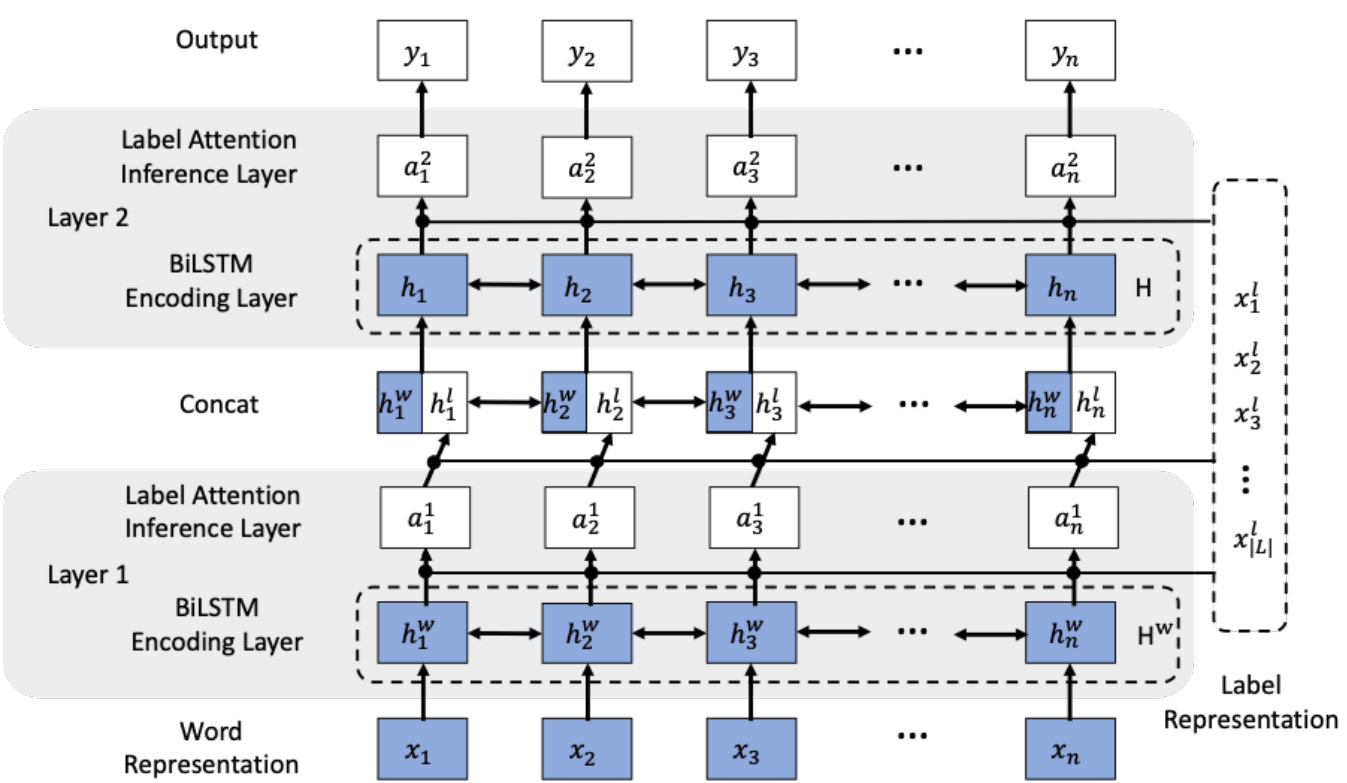
Figure 2: Architecture of hierarchically-refined label attention network.
图 2: 分层精炼标签注意力网络架构。
Neural CRF. There has been methods that aim to speed up neural CRF (Tu and Gimpel, 2018), and to solve the Markov constraint of neural CRF. In particular, Zhang et al. (2018b) predicts a sequence of labels as a sequence to sequence problem; Guo et al. (2019) further integrates global input information in encoding. Capturing non-local dependencies between labels, these methods, however, are slower compared with CRF. In contrast to these lines of work, our method is both asymptotically faster and empirically more accurate compared with neural CRF.
神经CRF。已有方法旨在加速神经CRF (Tu and Gimpel, 2018) 并解决其马尔可夫约束。例如,Zhang et al. (2018b) 将标签序列预测视为序列到序列问题;Guo et al. (2019) 进一步在编码中整合全局输入信息。这些方法虽能捕捉标签间的非局部依赖关系,但速度较CRF更慢。相比之下,我们的方法在渐进速度上更快,且实验精度优于神经CRF。
3 Baseline
3 基线
We implement BiLSTM-CRF and BiLSTMsoftmax baseline models with character-level features (Dos Santos and Zadrozny, 2014; Lample et al., 2016), which consist of a word representation layer, a sequence representation layer and a local softmax or CRF inference layer.
我们实现了带有字符级特征的BiLSTM-CRF和BiLSTMsoftmax基线模型 (Dos Santos and Zadrozny, 2014; Lample et al., 2016),该模型由词表示层、序列表示层以及局部softmax或CRF推理层组成。
3.1 Word Representation Layer
3.1 词表示层
Following Dos Santos and Zadrozny (2014) and Lample et al. (2016), we use character information for POS tagging. Given a word sequence
根据Dos Santos和Zadrozny (2014) 以及Lample等人 (2016) 的研究,我们使用字符信息进行词性标注。给定一个词序列
$w_{1},w_{2},...,w_{n}$ , where $c_{i j}$ denotes the $j$ th character in the $i$ th word, each $c_{i j}$ is represented using
$w_{1},w_{2},...,w_{n}$,其中$c_{i j}$表示第$i$个单词的第$j$个字符,每个$c_{i j}$用
$$
\mathbf{x}{i j}^{c}=\mathbf{e}^{c}(c_{i j})
$$
$$
\mathbf{x}{i j}^{c}=\mathbf{e}^{c}(c_{i j})
$$
where $\mathbf{e}^{c}$ denotes a character embedding lookup table.
其中 $\mathbf{e}^{c}$ 表示字符嵌入查找表。
We adopt BiLSTM for character encoding. $x_{i}^{c}$ denotes the output of character-level encoding.
我们采用BiLSTM进行字符编码。$x_{i}^{c}$表示字符级编码的输出。
A word is represented by concatenating its word embedding and its character representation:
一个单词通过拼接其词嵌入(word embedding)和字符表示(character representation)来表示:
$$
\mathbf{x}{i}=[\mathbf{e}^{w}(w_{i});\mathbf{x}_{i}^{c}]
$$
$$
\mathbf{x}{i}=[\mathbf{e}^{w}(w_{i});\mathbf{x}_{i}^{c}]
$$
where $\mathbf{e}^{w}$ denotes a word embedding lookup table.
其中 $\mathbf{e}^{w}$ 表示词嵌入查找表。
3.2 Sequence Representation Layer
3.2 序列表示层
For sequence encoding, the input is a sentence $\mathbf x={\mathbf x_{1},\cdot\cdot\cdot,\mathbf x_{n}}$ . Word representations are fed into a BiLSTM layer, yielding a sequence of forward hidden states ${\vec{\bf h}{1}^{w},\cdot\cdot\cdot,\vec{\bf h}{n}^{w}}$ $.\leftarrow.\leftarrow.$ equence of backward hidden states ${\dot{\mathbf{h}}{1}^{w},\cdot\cdot\cdot,\dot{\mathbf{h}}_{n}^{w}}$ , respectively. Finally, the two hidden states are concatenated for a final representation
对于序列编码,输入是一个句子 $\mathbf x={\mathbf x_{1},\cdot\cdot\cdot,\mathbf x_{n}}$。词表征被输入到一个双向长短期记忆网络(BiLSTM)层,分别生成前向隐藏状态序列 ${\vec{\bf h}{1}^{w},\cdot\cdot\cdot,\vec{\bf h}{n}^{w}}$ 和后向隐藏状态序列 ${\dot{\mathbf{h}}{1}^{w},\cdot\cdot\cdot,\dot{\mathbf{h}}_{n}^{w}}$。最终,这两个隐藏状态被拼接起来形成最终的表征。
$$
\begin{array}{r l}&{\mathbf{h}{i}^{w}=[\vec{\mathbf{h}{i}^{w}};\mathbf{h}{i}^{w}]}\ &{\mathbf{H}^{w}={\mathbf{h}{1}^{w},\cdot\cdot\cdot,\mathbf{h}_{n}^{w}}}\end{array}
$$
$$
\begin{array}{r l}&{\mathbf{h}{i}^{w}=[\vec{\mathbf{h}{i}^{w}};\mathbf{h}{i}^{w}]}\ &{\mathbf{H}^{w}={\mathbf{h}{1}^{w},\cdot\cdot\cdot,\mathbf{h}_{n}^{w}}}\end{array}
$$
3.3 Inference Layer
3.3 推理层
CRF. A CRF layer is used on top of the hidden vectors $\mathbf{H}^{w}$ . The conditional probabilities of label distribution sequences $y={y_{1},\cdot\cdot\cdot,y_{n}}$ is
CRF。在隐藏向量 $\mathbf{H}^{w}$ 之上使用了一个CRF层。标签分布序列 $y={y_{1},\cdot\cdot\cdot,y_{n}}$ 的条件概率为
$$
\begin{array}{r}{P(y|x)=\frac{\exp(\sum_{i}(\mathbf{W}{C R F}^{l_{i}}\mathbf{h_{i}}^{w}+b_{C R F}^{(l_{i-1},l_{i})}))}{\sum_{y^{\prime}}\exp(\sum_{i}(\mathbf{W}{C R F}^{l_{i}^{\prime}}\mathbf{h_{i}}^{w}+b_{C R F}^{(l_{i-1}^{\prime},l_{i}^{\prime})}))}}\end{array}
$$
$$
\begin{array}{r}{P(y|x)=\frac{\exp(\sum_{i}(\mathbf{W}{C R F}^{l_{i}}\mathbf{h_{i}}^{w}+b_{C R F}^{(l_{i-1},l_{i})}))}{\sum_{y^{\prime}}\exp(\sum_{i}(\mathbf{W}{C R F}^{l_{i}^{\prime}}\mathbf{h_{i}}^{w}+b_{C R F}^{(l_{i-1}^{\prime},l_{i}^{\prime})}))}}\end{array}
$$
Here $y^{\prime}$ represents an arbitrary label distribution qaunedn $\bar{\mathbf{W}}{C R F}^{l_{i}}$ ias bai ams osdpeelc ipfiarc atmo sapnedc .c to li, bCiR−F1 $b_{C R F}^{(l_{i-1}^{\prime},l_{i}^{\prime})}$ $l_{i-1}$ $l_{i}$
这里 $y^{\prime}$ 代表任意标签分布 qaunedn $\bar{\mathbf{W}}{CRF}^{l_{i}}$ ias bai ams osdpeelc ipfiarc atmo sapnedc .c to li, bCiR−F1 $b_{CRF}^{(l_{i-1}^{\prime},l_{i}^{\prime})}$ $l_{i-1}$ $l_{i}$
The first-order Viterbi algorithm is used to find the highest scored label sequence over an input word sequence during decoding.
一阶Viterbi算法用于在解码过程中找到输入词序列上得分最高的标签序列。
Softmax. Independent local softmax classification can give competitive result on sequence labeling (Reimers and Gurevych, 2017). For each node, $\mathbf{h}_{i}^{w}$ is fed to a softmax layer to find
Softmax。独立的局部softmax分类可以在序列标注任务中获得有竞争力的结果 (Reimers和Gurevych, 2017)。对于每个节点,$\mathbf{h}_{i}^{w}$被送入softmax层进行计算
$$
\hat{y}{i}=\mathrm{softmax}(\mathbf{W}\mathbf{h}_{i}^{w}+\mathbf{b})
$$
$$
\hat{y}{i}=\mathrm{softmax}(\mathbf{W}\mathbf{h}_{i}^{w}+\mathbf{b})
$$
where $\hat{y}{i}$ is the predicted label for $w_{i}$ ; W and b are the parameters for softmax layer.
其中 $\hat{y}{i}$ 是 $w_{i}$ 的预测标签;W 和 b 是 softmax 层的参数。
4 Label Attention Network
4 标签注意力网络
The structure of our refined label attention network is shown in Figure 2. We denote our model as BiLSTM-LAN (namely BiLSTM-label attention network) for the remaining of this paper. We use the same input word representations for BiLSTM-softmax, BiLSTM-CRF and BiLSTMLAN, as described in Section 3.1. Compared with the baseline models, BiLSTM-LAN uses a set of BiLSTM-LAN layers for both encoding and label prediction, instead of a set of traditional sequence encoding layers and an inference layer.
我们改进后的标签注意力网络结构如图2所示。在本文后续部分,我们将该模型称为BiLSTM-LAN(即BiLSTM标签注意力网络)。如第3.1节所述,我们为BiLSTM-softmax、BiLSTM-CRF和BiLSTM-LAN使用了相同的输入词表征。与基线模型相比,BiLSTM-LAN使用一组BiLSTM-LAN层同时进行编码和标签预测,而非使用传统的序列编码层和推理层组合。
4.1 Label Representation.
4.1 标签表示
Given the set of candidates output labels $L=$ ${l_{1},\cdots,l_{|L|}}$ , each label $l_{k}$ is represented using an embedding vector:
给定候选输出标签集合 $L=$ ${l_{1},\cdots,l_{|L|}}$ ,每个标签 $l_{k}$ 用嵌入向量表示:
$$
\mathbf{x}{k}^{l}=\mathbf{e}^{l}(l_{k})
$$
$$
\mathbf{x}{k}^{l}=\mathbf{e}^{l}(l_{k})
$$
where $\mathbf{e}^{l}$ denotes a label embedding lookup table. Label embeddings are randomly initialized and tuned during model training.
其中$\mathbf{e}^{l}$表示标签嵌入(label embedding)查找表。标签嵌入在模型训练期间随机初始化并调优。
4.2 BiLSTM-LAN Layer
4.2 BiLSTM-LAN 层
The model in Figure 2 consists of 2 BiLSTM-LAN layers. As discussed earlier, each BiLSTM-LAN layer is composed of a BiLSTM encoding sublayer and a label-attention inference sublayer. In paticular, the former is the same as the BiLSTM layer in the baseline model, while the latter uses multihead attention (Vaswani et al., 2017) to jointly encode information from the word representation subspace and the label representation subspace. For each head, we apply a dot-product attention with a scaling factor to the inference component, deriving label distributions for BiLSTM hidden states and label embeddings.
图 2 中的模型包含 2 个 BiLSTM-LAN 层。如前所述,每个 BiLSTM-LAN 层由 BiLSTM 编码子层和标签注意力推理子层组成。其中,前者与基线模型中的 BiLSTM 层相同,后者则采用多头注意力机制 (Vaswani et al., 2017) 联合编码来自词表示子空间和标签表示子空间的信息。对于每个注意力头,我们在推理组件中应用带缩放因子的点积注意力,从而为 BiLSTM 隐藏状态和标签嵌入生成标签分布。
BiLSTM Encoding Sublayer. Denote the input to each layer as $\mathbf{x}={\mathbf{x}{1},\mathbf{x}{2},...,\mathbf{x}{n}}$ . BiL- STM (Section 3.2) is used to calculate $\mathbf{H}^{w}\in$ $\mathbb{R}^{n\times d{h}}$ , where $n$ and $d_{h}$ denote the word sequence length and BiLSTM hidden size (same as the dimension of label embedding), respectively.
BiLSTM 编码子层。将每层的输入表示为 $\mathbf{x}={\mathbf{x}{1},\mathbf{x}{2},...,\mathbf{x}{n}}$。使用 BiLSTM (第 3.2 节) 计算 $\mathbf{H}^{w}\in$ $\mathbb{R}^{n\times d{h}}$,其中 $n$ 和 $d_{h}$ 分别表示词序列长度和 BiLSTM 隐藏层大小 (与标签嵌入维度相同)。
Label-Attention Inference Sublayer. For the label-attention inference sublayer, the attention mechanism produces an attention matrix $_{\alpha}$ consisting of a potential label distribution for each word. We define $\mathbf{Q}=\mathbf{H}^{w}$ , $\mathbf{K}=\mathbf{V}=\mathbf{x}^{l}$ . $\mathbf{x}^{l}\in\mathbf{\Psi}$ $\mathbb{R}^{|L|\times d_{h}}$ is the label set representation, where $|L|$ is the total number of labels. As shown in Figure 2, outputs are calculated by
标签注意力推理子层。在标签注意力推理子层中,注意力机制生成一个由每个单词的潜在标签分布组成的注意力矩阵 $_{\alpha}$。我们定义 $\mathbf{Q}=\mathbf{H}^{w}$,$\mathbf{K}=\mathbf{V}=\mathbf{x}^{l}$。$\mathbf{x}^{l}\in\mathbf{\Psi}$ $\mathbb{R}^{|L|\times d_{h}}$ 是标签集表示,其中 $|L|$ 是标签总数。如图 2 所示,输出通过以下方式计算:
$$
\begin{array}{l}{{\displaystyle{\bf H}^{l}=\mathrm{attention}({\bf Q},{\bf K},{\bf V})=\alpha{\bf V}}}\ {{\displaystyle~\alpha=\mathrm{softmax}(\frac{{\bf Q}{\bf K}^{T}}{\sqrt{d_{h}}})}}\end{array}
$$
$$
\begin{array}{l}{{\displaystyle{\bf H}^{l}=\mathrm{attention}({\bf Q},{\bf K},{\bf V})=\alpha{\bf V}}}\ {{\displaystyle~\alpha=\mathrm{softmax}(\frac{{\bf Q}{\bf K}^{T}}{\sqrt{d_{h}}})}}\end{array}
$$
Instead of the standard attention mechanism above, it can be beneficial to use multi-head for capturing multiple possible of potential label distributions in parallel.
不同于上述标准注意力机制,使用多头注意力 (multi-head) 可以并行捕获潜在标签分布的多种可能性。
$$
\begin{array}{c}{\mathbf{H}^{l}=\operatorname{concat}(\mathrm{head},\boldsymbol{\cdot}\boldsymbol{\cdot}\boldsymbol{\cdot},\mathrm{head}{k})+\mathbf{H}^{w}}\ {\mathrm{head}{i}=\mathrm{attention}(\mathbf{Q}\mathbf{W}{i}^{Q},\mathbf{K}\mathbf{W}{i}^{K},\mathbf{V}\mathbf{W}_{i}^{V})}\end{array}
$$
$$
\begin{array}{c}{\mathbf{H}^{l}=\operatorname{concat}(\mathrm{head},\boldsymbol{\cdot}\boldsymbol{\cdot}\boldsymbol{\cdot},\mathrm{head}{k})+\mathbf{H}^{w}}\ {\mathrm{head}{i}=\mathrm{attention}(\mathbf{Q}\mathbf{W}{i}^{Q},\mathbf{K}\mathbf{W}{i}^{K},\mathbf{V}\mathbf{W}_{i}^{V})}\end{array}
$$
where WQ $\begin{array}{r}{\mathbf{W}{i}^{Q} \in~\mathbb{R}^{d_{h}\times\frac{d_{h}}{k}}}\end{array}$ , $\begin{array}{r}{\mathbf{W}{i}^{K} \in~\mathbb{R}^{d_{h}\times\frac{d_{h}}{k}}}\end{array}$ and $\mathbf{W}{i}^{V}\in\mathbb{R}^{d_{h}\times\frac{d_{h}}{k}}$ are parameters to be learned during the training, $k$ is the number of parallel heads.
其中 WQ $\begin{array}{r}{\mathbf{W}{i}^{Q} \in~\mathbb{R}^{d_{h}\times\frac{d_{h}}{k}}}\end{array}$、 $\begin{array}{r}{\mathbf{W} {i}^{K} \in~\mathbb{R}^{d_{h}\times\frac{d_{h}}{k}}}\end{array}$ 和 $\mathbf{W} {i}^{V}\in\mathbb{R}^{d_{h}\times\frac{d_{h}}{k}}$ 是训练过程中需要学习的参数,$k$ 表示并行注意力头的数量。
The final representation for each BiLSTM-LAN layer is the concatenation of BiLSTM hidden states and attention outputs :
每个BiLSTM-LAN层的最终表示是BiLSTM隐藏状态和注意力输出的拼接:
$$
\mathbf{H}=[\mathbf{H}^{w};\mathbf{H}^{l}]
$$
$$
\mathbf{H}=[\mathbf{H}^{w};\mathbf{H}^{l}]
$$
$\mathbf{H}$ is then fed to a subsequent BiLSTM-LAN layer as input, if any.
$\mathbf{H}$ 随后作为输入馈送到后续的 BiLSTM-LAN 层(如果有的话)。
Output. In the last layer, BiLSTM-LAN directly predicts the label of each word based on the attention weights.
输出。在最后一层,BiLSTM-LAN 基于注意力权重直接预测每个单词的标签。
$$
\left[\begin{array}{c}{\hat{y_{1}}^{1}\cdot\cdot\cdot\hat{y_{1}}^{\left|L\right|}}\ {\cdot\cdot\cdot\cdot}\ {\cdot\cdot\cdot}\ {\cdot\cdot\cdot\cdot}\ {\hat{y_{i}}^{1}\cdot\cdot\cdot\cdot\hat{y_{i}}^{\left|L\right|}}\end{array}\right]=\alpha
$$
$$
\left[\begin{array}{c}{\hat{y_{1}}^{1}\cdot\cdot\cdot\hat{y_{1}}^{\left|L\right|}}\ {\cdot\cdot\cdot\cdot}\ {\cdot\cdot\cdot}\ {\cdot\cdot\cdot\cdot}\ {\hat{y_{i}}^{1}\cdot\cdot\cdot\cdot\hat{y_{i}}^{\left|L\right|}}\end{array}\right]=\alpha
$$
$$
\hat{y_{i}}=\mathrm{argmax}{j}(\hat{y_{i}}^{1},...,\hat{y_{i}}^{n})
$$
$$
\hat{y_{i}}=\mathrm{argmax}{j}(\hat{y_{i}}^{1},...,\hat{y_{i}}^{n})
$$
where $\hat{y_{i}}^{j}$ denotes the $j$ th candidate label for the $i$ th word and $\hat{y}_{i}$ is the predicted label for ith word in the sequence.
其中 $\hat{y_{i}}^{j}$ 表示第 $i$ 个单词的第 $j$ 个候选标签,$\hat{y}_{i}$ 是该序列中第 $i$ 个单词的预测标签。
4.3 Training
4.3 训练
BiLSTM-LAN can be trained by standard backpropagation using the log-likelihood loss. The training object is to minimize the cross-entropy between $y_{i}$ and $\hat{y}_{i}$ for all labeled gold-standard sentences. For each sentence,
BiLSTM-LAN 可通过标准反向传播使用对数似然损失进行训练。训练目标是最小化所有标注黄金标准句子的 $y_{i}$ 与 $\hat{y}_{i}$ 之间的交叉熵。对于每个句子,
$$
L=-\sum_{i}\sum_{j}y_{i}^{j}\log\hat{y}_{i}^{j}
$$
$$
L=-\sum_{i}\sum_{j}y_{i}^{j}\log\hat{y}_{i}^{j}
$$
where $i$ is the word index, $j$ is the index of labels for each word.
其中 $i$ 是单词索引,$j$ 是每个单词的标签索引。
4.4 Complexity
4.4 复杂度
For decoding, the asymptotic time complexity is $O(|L|^{2}n)$ and $O(|L|n)$ for BiLSTM-CRF and BiLSTM-LAN, respectively, where $|L|$ is the total number of labels and $n$ is the sequence length. Compared with BiLSTM-CRF, BiLSTMLAN can significantly increase the speed for sequence labeling, especially for CCG super tagging, where the sequence length can be much smaller than the total number of labels.
在解码阶段,BiLSTM-CRF和BiLSTM-LAN的渐进时间复杂度分别为 $O(|L|^{2}n)$ 和 $O(|L|n)$ ,其中 $|L|$ 是标签总数, $n$ 是序列长度。与BiLSTM-CRF相比,BiLSTM-LAN能显著提升序列标注速度,尤其对于CCG超标注任务(当序列长度远小于标签总数时)效果更为明显。
4.5 BiLSTM-LAN and BiLSTM-softmax
4.5 BiLSTM-LAN 和 BiLSTM-softmax
As mentioned in the introduction, a singlelayer BiLSTM-LAN is identical to a single-layer BiLSTM-softmax sequence labeling model. In particular, the BiLSTM-softmax model is given by Eq 1. In a BiLSTM-LAN model, we arrange the set of label embeddings into a matrix as follows:
如引言所述,单层BiLSTM-LAN与单层BiLSTM-softmax序列标注模型结构相同。具体而言,BiLSTM-softmax模型由公式1给出。在BiLSTM-LAN模型中,我们将标签嵌入集按如下方式排列为矩阵:
$$
\mathbf{x}^{l}=[x_{1}^{l};x_{2}^{l};...,x_{|L|}^{l}]
$$
$$
\mathbf{x}^{l}=[x_{1}^{l};x_{2}^{l};...,x_{|L|}^{l}]
$$
A naive attention model over $\mathrm{X}$ has:
在 $\mathrm{X}$ 上的朴素注意力模型具有:
$$
\pmb{\alpha}=\mathrm{softmax}(\mathbf{H}\mathbf{x}^{l})
$$
$$
\pmb{\alpha}=\mathrm{softmax}(\mathbf{H}\mathbf{x}^{l})
$$
It is thus straightforward to see that the label embedding matrix $\mathbf{x}^{l}$ corresponds to the weight matrix $\mathbf{W}$ is $\operatorname{Eq}1$ , and the distribution $_{\alpha}$ corresponds to y in $\operatorname{Eq}1$ .
因此可以直观看出,标签嵌入矩阵 $\mathbf{x}^{l}$ 对应的权重矩阵 $\mathbf{W}$ 满足 $\operatorname{Eq}1$,而分布 $_{\alpha}$ 对应于 $\operatorname{Eq}1$ 中的 y。
5 Experiments
5 实验
We empirically compare BiLSTM-CRF, BiLSTM-softmax and BiLSTM-LAN using different sequence labelling tasks, including English POS tagging, multilingual POS tagging, NER and CCG super tagging.
我们通过实证比较了BiLSTM-CRF、BiLSTM-softmax和BiLSTM-LAN在不同序列标注任务中的表现,包括英语词性标注、多语言词性标注、命名实体识别(NER)和组合范畴语法(CCG)超级标注。
Table 1: Data statistics. l:label, s:sentence, t:tokens.
表 1: 数据统计。l:标签,s:句子,t:token。
| Data | training | dev | test | |
|---|---|---|---|---|
| WSJ | # | 45 | 45 | 45 |
| #S | 38,219 | 5,527 | 5,462 | |
| # | 912,344 | 131,768 | 129,654 | |
| UD-en | # | 50 | 50 | 49 |
| #S | 12,544 | 2,003 | 2,078 | |
| # | 204,607 | 25,150 | 25,097 | |
| OntoNotes | # | 18 | 18 | 18 |
| #S | 59,924 | 8,528 | 8,262 | |
| # | 1,088,503 | 147,724 | 152,728 | |
| CCGBank | # | 426 | 323 | 348 |
| #S | 39,604 | 1,913 | 2,407 | |
| # | 929,552 | 45,422 | 55,371 |
Table 2: WSJ development set. E: label embedding size, H: hidden size, L: number of layers.
表 2: WSJ开发集。E: 标签嵌入大小,H: 隐藏层大小,L: 层数。
| 模型 | H#/# T# | Acc | #Param |
|---|---|---|---|
| 200 BiLSTM-CRF | 1 | 97.56 | 5.1M |
| 400 1 | 97.57 | 5.5M | |
| 400 2 | 97.57 | 6.4M | |
| 400 3 | 97.52 | 7.4M | |
| 600 2 | 97.57 | 8.2M | |
| BiLSTM-LAN | 600 3 3 | 97.50 | 10.4M |
| 200 400 | 97.53 | 5.7M | |
| 2 400 | 97.57 97.63 | 8.1M 10.0M | |
| 3 400 4 | 97.60 | 12.2M | |
| 600 3 | 97.62 | ||
| 16.5M |
Table 3: Effect of attention layer. $\dagger$ denotes the model without attention sublayers except for the last layer.
表 3: 注意力层效果。$\dagger$ 表示除最后一层外不含注意力子层的模型。
| 模型 | 准确率 (%) |
|---|---|
| BiLSTM-CRF | 97.57 |
| BiLSTM-softmax | 97.58 |
| 97.59 | |
| BiLSTM-LAN | 97.65 |
5.1 Dataset
5.1 数据集
For English POS tagging, we use the Wall Street Journal (WSJ) portion of the Penn Treebank (PTB) (Marcus et al., 1993), which has 45 POS tags. We adopt the same partitions used by previous work (Manning, 2011; Yang et al., 2018), selecting sections 0-18 as the training set, sections 19-21 as the development set and sections 22-24 as the test set. For multilingual POS tagging, we use treebanks from Universal Dependencies(UD) v2.2 (Silveira et al., 2014; Nivre et al., 2018) with the standard splits, choosing 8 resource-rich languages in our experiments. For NER, we use the OntoNotes 5.0 (Hovy et al., 2006; Pradhan et al., 2013). Following previous work,we adopt the official OntoNotes data split used for co-reference resolution in the CoNLL-2012 shared task (Pradhan et al., 2012). We train our CCG super tagging model on CCGBank (Hocken maier and Steedman, 2007). Sections 2-21 are used for training, section 0 for development and section 23 as the test set. The performance is calculated on the 425 most frequent labels. Table 1 shows the numbers of sentences, tokens and labels for training, development and test, respectively.
对于英语词性标注任务,我们采用宾州树库(PTB) (Marcus等人,1993)中的《华尔街日报》(WSJ)部分,包含45种词性标签。沿用前人工作(Manning, 2011; Yang等人, 2018)的划分方式:选取0-18章节作为训练集,19-21章节作为开发集,22-24章节作为测试集。在多语言词性标注任务中,我们使用通用依存树库(UD)v2.2 (Silveira等人,2014; Nivre等人,2018)的标准划分,实验中选取了8种资源丰富的语言。命名实体识别任务采用OntoNotes 5.0 (Hovy等人,2006; Pradhan等人,2013)数据集,遵循CoNLL-2012共享任务(Pradhan等人,2012)中用于共指消解的官方划分方案。CCG超标注模型训练基于CCGBank (Hockenmaier和Steedman,2007)数据集,其中2-21章节用于训练,0章节用于开发,23章节作为测试集,性能评估基于425个高频标签。表1分别展示了训练集、开发集和测试集的句子数、token数及标签数量。
Table 4: Comparison of the training time for one iteration and decoding speed. st indicates sentences
表 4: 单次迭代训练时间与解码速度对比。st表示句子
| 模型 | 训练(s) | 测试(st/s) |
|---|---|---|
| BiLSTM-CRF (POS) | 181.32 | 781.90 |
| BiLSTM-LAN (POS) | 128.75 | 805.32 |
| BiLSTM-CRF (CCG) | 884.67 | 599.18 |
| BiLSTM-LAN (CCG) | 369.98 | 713.70 |
5.2 Settings
5.2 设置
Hyper-Parameters. We use 100-dimensional GloVe (Pennington et al., 2014) word embeddings for English POS tagging (WSJ, UD $\mathrm{v}2.2\mathrm{EN}$ and name entity recognition, 300-dimensional Glove word embeddings for CCG super tagging and 64- dimensional Polyglot (Al-Rfou et al., 2013) word embeddings for multilingual POS tagging. The detail values of the hyper-parameters for all experiments are summarized in Appendix A.
超参数 (Hyper-Parameters)。对于英语词性标注 (WSJ, UD v2.2EN) 和命名实体识别任务,我们使用 100 维 GloVe (Pennington et al., 2014) 词向量;CCG 超标注任务使用 300 维 GloVe 词向量;多语言词性标注任务使用 64 维 Polyglot (Al-Rfou et al., 2013) 词向量。所有实验的超参数具体值汇总于附录 A。
Evaluation. F-1 score are used for NER. Other tasks are evaluated based on the accuracy. We repeat the same experiment five times with the same hyper parameters and report the max accuracy, average accuracy and standard deviation for POS tagging. For fair comparison, all experiments are implemented in ${\mathrm{NCRF{++}}}$ (Yang and Zhang, 2018) and conducted using a GeForce GTX 1080Ti with 11GB memory.
评估。命名实体识别(NER)采用F-1分数作为评估指标,其他任务基于准确率进行评估。我们使用相同超参数重复五次实验,针对词性标注(POS tagging)报告最高准确率、平均准确率及标准差。为保证公平对比,所有实验均在 ${\mathrm{NCRF{++}}}$ (Yang and Zhang, 2018)框架下实现,并在配备11GB显存的GeForce GTX 1080Ti显卡上运行。
5.3 Development Experiments
5.3 开发实验
We report a set of WSJ development experiments to show our investigation on key configurations of BiLSTM-LAN and BiLSTM-CRF.
我们报告了一组WSJ开发实验,以展示对BiLSTM-LAN和BiLSTM-CRF关键配置的研究。
Label embedding size. Table 2 shows the effect of the label embedding size. Notable improvement can be achieved when the label embedding size increases from 200 to 400 in our model, but the accuracy does not further increase when the size increases beyond 400. We fix the label embedding size to 400 for our model.
标签嵌入维度。表 2 展示了标签嵌入维度的影响。当标签嵌入维度从 200 增加到 400 时,我们的模型取得了显著提升,但超过 400 后准确率不再继续提高。我们将模型的标签嵌入维度固定为 400。
Number of Layers. For BiLSTM-CRF, previous work has shown that one BiLSTM layer is the most effecitve for POS tagging (Ma and Hovy, 2016; Yang et al., 2018). Table 2 compares differ- ent numbers of BiLSTM layers and hidden sizes.
层数。对于BiLSTM-CRF,先前研究表明单层BiLSTM在词性标注任务中效果最佳 (Ma and Hovy, 2016; Yang et al., 2018)。表2比较了不同BiLSTM层数和隐藏层大小的效果。
Table 5: Result for POS tagging on WSJ. $\dagger$ Yang et al. (2018) and $^\ddag$ Yasunaga et al. (2018) are baseline models re-implemented in ${\mathrm{NCRF{++}}}$ (Yang and Zhang, 2018). Our results are same as Table 6 of Yang et al. (2018).
表 5: WSJ词性标注结果。$\dagger$ Yang等人(2018)和$^\ddag$ Yasunaga等人(2018)是在${\mathrm{NCRF{++}}}$ (Yang和Zhang, 2018)中重新实现的基线模型。我们的结果与Yang等人(2018)的表6相同。
| 模型 | 均值±标准差 | 最大值 |
|---|---|---|
| BiLSTM-CRFt | 97.47±0.02 | 97.49 |
| BiLSTM-CRF | 97.50±0.03 | 97.51 |
| 97.48±0.02 | 97.51 | |
| BiLSTM-LAN | 97.58±0.04 | 97.65 |
Table 6: Main results on WSJ.
表 6: WSJ 主要实验结果
| 模型 | 准确率 |
|---|---|
| Plank et al. (2016) | 97.22 |
| Huang et al. (2015) Ma and Hovy (2016) | 97.55 |
| Liu et al. (2017) | 97.55 97.53 |
| Yang et al. (2018) | 97.51 |
| Zhang et al. (2018c) | 97.55 |
| Yasunaga et al. (2018) | 97.58 |
| Xin et al. (2018) | 97.58 |
| Transformer-softmax (Guo et al., 2019) | 97.04 |
| BiLSTM-softmax (Yang et al., 2018) | 97.51 |
| BiLSTM-CRF (Yang et al., 2018) | 97.51 |
| BiLSTM-LAN | 97.65 |
As can be seen, a multi-layer model with larger hidden sizes does not give significantly better results compared to a 1-layer model with a hidden size of 400. We thus chose the latter for the final model.
可以看出,与隐藏层大小为400的单层模型相比,具有更大隐藏层大小的多层模型并未带来显著更好的结果。因此我们最终选择了后者作为模型架构。
For BiLSTM-LAN, each layer learns a more abstract representation of word and label distribution sequences. As shown in Table 2, for POS tagging, it is effective to capture label dependencies using two layers. More layers do not empirically improve the performance. We thus set the final number of layers to 3.
对于 BiLSTM-LAN,每一层都学习单词和标签分布序列的更抽象表示。如表 2 所示,对于词性标注任务,使用两层能有效捕捉标签依赖关系。实验表明,增加更多层数并不能提升性能。因此我们最终将层数设置为 3。
The effectiveness of Model Structure. To evaluate the effect of BiLSTM-LAN layers, we conduct ablation experiments as shown in Table 3. In BiLSTM-LAN w/o attention, we remove the attention inference sublayers from BiLSTMLAN except for the last BiLSTM-LAN layer. This model is reminiscent to BiLSTM-softmax except that the output is based on label embeddings. It gives an accuracy slightly higher than that of LSTM-softmax, which demonstrates the advantage of label embeddings. On the other hand, it significantly under performs BiLSTMLAN ( $p$ -value $<0.01$ ), which shows the advantage of hierarchically-refined label distribution sequence encoding.
模型结构的有效性。为评估BiLSTM-LAN层的作用,我们进行了如表3所示的消融实验。在BiLSTM-LAN w/o attention中,我们移除了除最后一层外所有BiLSTM-LAN层的注意力推断子层。该模型类似于BiLSTM-softmax,区别在于其输出基于标签嵌入(label embeddings)。其准确率略高于LSTM-softmax,证明了标签嵌入的优势。但该模型性能显著低于完整版BiLSTM-LAN ( $p$ -值 $<0.01$ ),这体现了分层精炼的标签分布序列编码的优越性。
Model Size vs CRF. Table 2 also compares the effect of model sizes. We observe that: (1) As the model size increases, both BiLSTM-CRF and BiLSTM-LAN see a peak point beyond which further increase of model size does not bring better results, which is consistent with observations from prior work, demonstrating that the number of parameters is not the decisive factor to model accuracy; and (2) the best-performing BiLSTM-LAN model size is comparable to that of the BiLSTMCRF model size, which indicates that the model structure is more important for the better accuracy of BiLSTM-LAN.
模型规模与CRF对比。表2还比较了模型规模的影响。我们观察到:(1) 随着模型规模增大,BiLSTM-CRF和BiLSTM-LAN都会出现峰值点,超过该点后继续增加模型规模不会带来更好结果,这与先前研究的观察一致,表明参数量并非模型精度的决定性因素;(2) 性能最佳的BiLSTM-LAN模型规模与BiLSTM-CRF相当,这表明模型结构对BiLSTM-LAN的精度提升更为重要。
Table 7: Multilingual POS tagging result on UD $\mathrm{v}2.2$ treebanks, compared on 8 resource-rich languages.
| CS | da | en | fr | nl | no | pt | SV |
|---|---|---|---|---|---|---|---|
| BiLSTM-CRF | |||||||
| mean | 98.42 | 95.77 | 95.41 | 96.94 | 94.65 | 97.07 | 97.78 |
| ± std | 0.03 | 0.12 | 0.06 | 0.08 | 0.11 | 0.11 | 0.04 |
| (Yasunaga et al.,2018) training(s) | 268.74 | 18.17 | 58.20 | 70.10 | 44.49 | 56.06 | 51.59 |
| BiLSTM-softmax | |||||||
| mean | 98.48 | 95.90 | 95.36 | 97.01 | 94.76 | 97.26 | 97.78 |
| ± std | 0.04 | 0.09 | 0.17 | 0.09 | 0.17 | 0.03 | 0.05 |
| training(s) | 129.14 | 9.27 | 25.02 | 33.65 | 23.00 | 28.84 | 23.13 |
| BiLSTM-LAN | |||||||
| mean | 98.75 | 96.26 | 95.59 | 97.28 | 94.94 | 97.59 | 98.04 |
| ± std | 0.02 | 0.12 | 0.13 | 0.08 | 0.11 | 0.04 | 0.04 |
| training(s) | 165.64 | 11.32 | 33.04 | 40.48 | 29.71 | 37.06 | 27.48 |
表 7: UD $\mathrm{v}2.2$ 树库上8种资源丰富语言的跨语言词性标注结果对比。
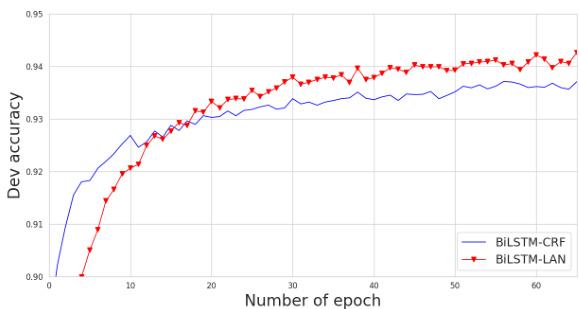
Figure 3: Training on the WSJ development set.
图 3: 在WSJ开发集上的训练
Speed vs CRF. Table 4 shows a comparison of training and decoding speeds. BiLSTM-LAN processes 805 and 714 sentences per second on the WSJ and CCGBank development data, respectively, outperforming BiLSTM-CRF by $3%$ and $19%$ , respectively. The larger speed improvement on CCGBank shows the benefit of lower asymptotic complexity, as discussed in Section 4.
速度与CRF对比。表4展示了训练和解码速度的比较。BiLSTM-LAN在WSJ和CCGBank开发数据上分别每秒处理805和714个句子,分别比BiLSTM-CRF快3%和19%。在CCGBank上更大的速度提升显示了较低渐近复杂度的优势,如第4节所述。
Training vs CRF. Figure 3 presents the training curves on the WSJ development set. At the beginning, BiLSTM-LAN converges slower than BiLSTM-CRF, which is likely because BiLSTMLAN has more complex layer structures for label embedding and attention. After around 15 training iterations, the accuracy of BiLSTM-LAN on the development sets becomes increasingly higher than BiLSTM-CRF. This demonstrates the effect of label embeddings, which allows more structured knowledge to be learned in modeling.
训练与CRF对比。图3展示了在WSJ开发集上的训练曲线。初期,BiLSTM-LAN的收敛速度慢于BiLSTM-CRF,这可能是由于BiLSTM-LAN具有更复杂的标签嵌入和注意力层结构。经过约15次训练迭代后,BiLSTM-LAN在开发集上的准确率逐渐超越BiLSTM-CRF。这证明了标签嵌入的效果,它能在建模过程中学习更具结构化的知识。
5.4 Final Results
5.4 最终结果
WSJ. Table 5 shows the final POS tagging results on WSJ. Each experiment is repeated 5 times. BiLSTM-LAN gives significant accuracy improvements over both BiLSTM-CRF and BiLSTM-softmax $(p<0.01)$ , which is consistent with observations on development experiments.
WSJ。表5展示了在WSJ上的最终词性标注结果。每个实验重复5次。BiLSTM-LAN相比BiLSTM-CRF和BiLSTM-softmax取得了显著的准确率提升$(p<0.01)$,这与开发实验的观察结果一致。
Table 6 compares our model with topperforming methods reported in the literature. In particular, Huang et al. (2015) use BiLSTM-CRF. Ma and Hovy (2016), Liu et al. (2017) and Yang et al. (2018) explore character level representations on BiLSTM-CRF. Zhang et al. (2018c) use S-LSTM-CRF, a graph recurrent network encoder. Yasunaga et al. (2018) demonstrate that adversarial training can improve the tagging accuracy. Xin et al. (2018) proposed a compositional character-to-word model combined with LSTMCRF. BiLSTM-LAN gives highly competitive result on WSJ without training on external data.
表 6 将我们的模型与文献中报道的顶级方法进行了比较。具体而言,Huang 等人 (2015) 使用了 BiLSTM-CRF。Ma 和 Hovy (2016)、Liu 等人 (2017) 以及 Yang 等人 (2018) 探索了 BiLSTM-CRF 上的字符级表示。Zhang 等人 (2018c) 使用了 S-LSTM-CRF,一种图循环网络编码器。Yasunaga 等人 (2018) 证明了对抗训练可以提高标注准确率。Xin 等人 (2018) 提出了一种结合 LSTMCRF 的组合式字符到词模型。BiLSTM-LAN 在未使用外部数据训练的情况下,在 WSJ 上取得了极具竞争力的结果。
Universal Dependencies(UD) v2.2. We design a multilingual experiment to compare BiLSTMsoftmax, BiLSTM-CRF (strictly following Yasunaga et al. (2018) 1, which is the state-of-theart on multi-lingual POS tagging) and BiLSTMLAN. The accuracy and training speeds are shown in Table 7. Our model outperforms all the baselines on all the languages. The improvements are statistically significant for all the languages $(p<0.01)$ , suggesting that BiLSTM-LAN is generally effective across languages.
Universal Dependencies (UD) v2.2。我们设计了一项多语言实验,比较 BiLSTM-softmax、BiLSTM-CRF (严格遵循 Yasunaga 等人 (2018) [1] 的方法,该方法在多语言词性标注任务上达到最优性能) 和 BiLSTM-LAN。准确率和训练速度如表 7 所示。我们的模型在所有语言上均优于基线方法。对于所有语言,改进均具有统计学显著性 $(p<0.01)$ ,表明 BiLSTM-LAN 在不同语言中普遍有效。
OntoNotes 5.0. In NER, BiLSTM-CRF is widely used, because local dependencies between neighboring labels relatively more important that POS tagging and CCG super tagging. BiLSTMLAN also significantly outperforms BiLSTMCRF by 1.17 F1-score $(p<0.01)$ . Table 8 compares BiLSTM-LAN to other published results on
OntoNotes 5.0。在命名实体识别(NER)任务中,BiLSTM-CRF被广泛使用,因为相邻标签间的局部依赖关系比词性标注(POS tagging)和组合范畴语法超标注(CCG super tagging)更为重要。BiLSTM-LAN以1.17个F1值的显著优势超越BiLSTM-CRF $(p<0.01)$ 。表8将BiLSTM-LAN与其他已发表成果进行了对比
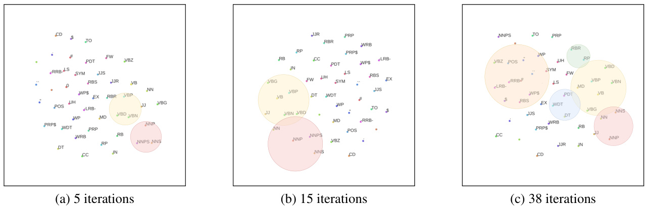
Figure 4: t-SNE plot of label embeddings after different numbers of training iterations.
图 4: 不同训练迭代次数后标签嵌入的 t-SNE 可视化图。
OntoNotes 5.0. Durrett and Klein (2014) propose a joint model for co reference resolution, entity linking and NER. Chiu and Nichols (2016) use a BiLSTM with CNN character encoding. Shen et al. (2017) introduce active learning to get better performance. Strubell et al. (2017) present an iterated dilated convolutions, which is a faster alternative to BiLSTM. Ghaddar and Langlais (2018) demonstrate that lexical features are actually quite useful for NER. Clark et al. (2018) present a cross-view training for neural sequence models. BiLSTM-LAN obtains highly competitive results compared with various of top-performance models without training on external data.
OntoNotes 5.0。Durrett和Klein (2014) 提出了一个用于共指消解、实体链接和命名实体识别(NER)的联合模型。Chiu和Nichols (2016) 使用带有CNN字符编码的BiLSTM。Shen等人 (2017) 引入主动学习以获得更好的性能。Strubell等人 (2017) 提出了一种迭代扩张卷积,这是BiLSTM的一种更快替代方案。Ghaddar和Langlais (2018) 证明了词汇特征对NER实际上非常有用。Clark等人 (2018) 提出了一种用于神经序列模型的跨视图训练方法。BiLSTM-LAN在不使用外部数据训练的情况下,与各种顶级性能模型相比获得了极具竞争力的结果。
CCGBank. In CCG super tagging, the major challenge is a larger set of lexical tags $|L|$ and supertag constraints over long distance dependencies. As shown in Table 9, BiLSTMLAN significantly outperforms both BiLSTMsoftmax and BiLSTM-CRF $(p_{0}0.01)$ , showing the advantage of LAN. Xu et al. (2015) and Vaswani et al. (2016a) explore BiRNN-softmax and BiLSTM-softmax, respectively. Søgaard and Goldberg (2016) present a multi-task learning architecture with BiRNN to improve the performance. Lewis et al. (2016) train BiLSTM-softmax using tri-training. Vaswani et al. (2016b) combine a LSTM language model and BiLSTM over the supertags. Tu and Gimpel (2019) introduce the inference network (Tu and Gimpel, 2018) in CCG super tagging to speed up the training and decoding for BiLSTM-CRF. Compared with these methods, BiLSTM-LAN obtains new state-of-theart results on CCGBank, matching the tri-training performance of Lewis et al. (2016), without training on external data.
CCGBank。在CCG超标注任务中,主要挑战在于更大的词汇标签集$|L|$以及长距离依赖上的超标注约束。如表9所示,BiLSTMLAN显著优于BiLSTMsoftmax和BiLSTM-CRF$(p_{0}0.01)$,展现了LAN的优势。Xu等人(2015)和Vaswani等人(2016a)分别探索了BiRNN-softmax和BiLSTM-softmax。Søgaard和Goldberg(2016)提出采用BiRNN的多任务学习架构来提升性能。Lewis等人(2016)通过三重训练(tri-training)训练BiLSTM-softmax。Vaswani等人(2016b)将LSTM语言模型与基于超标注的BiLSTM相结合。Tu和Gimpel(2019)在CCG超标注中引入推断网络(Tu和Gimpel,2018)以加速BiLSTM-CRF的训练和解码。与这些方法相比,BiLSTM-LAN在CCGBank上取得了新的最先进成果,在不使用外部数据训练的情况下,达到了Lewis等人(2016)三重训练的性能水平。
Table 8: F1-scores on the OntoNotes 5.0 test set. * denotes semi-supervised and multi-task learning.
表 8: OntoNotes 5.0 测试集上的 F1 分数。* 表示半监督和多任务学习。
| Model | F1 |
|---|---|
| Durrett and Klein (2014) Chiu and Nichols (2016) | 84.04 86.28 |
| Shen et al. (2017) Strubell et al. (2017) Ghaddar and Langlais (2018) | 86.52 86.84 87.95 |
| Clark et al. (2018) 米 BiLSTM-softmax (Strubell et al., 2017) BiLSTM-CRF (Strubell et al., 2017) | 88.81 83.76 |
Table 9: Super tagging accuracy on CCGbank test set. * indicates that further gains follow from semisupervised tri-training (improving the accuracy from $94.3%$ to $94.7%$ ).
表 9: CCGbank测试集上的超级标注准确率。*表示通过半监督三重训练可进一步提升(准确率从$94.3%$提高到$94.7%$)。
| 模型 | 准确率(%) |
|---|---|
| Xu et al.(2015) | 93.0 |
| Sogaard and Goldberg (2016) | 93.3 |
| Vaswaniet al.(2016a) | 94.2 |
| Lewis et al. (2016) | 94.3 |
| Lewis et al. (2016) | 94.7* |
| Vaswani et al.(2016b) | 94.5 |
| Tu and Gimpel (2019) | 94.4 |
| BiLSTM-softmax | 94.1 |
| BiLSTM-CRF | 94.1 |
| BiLSTM-LAN | 94.7 |
6 Discussion
6 讨论
Visualization. A salient advantage of LAN is more interpret able models. We visualize the label embeddings as well as label attention weights for POS tagging. We use t-SNE to visualize the 45 different English POS tags (WSJ) on a 2D map after 5, 15, 38 training iteration, respectively. Each dot represents a label embedding. As can be seen in Figure 4, label embeddings are increasingly more meaningful during training. Initially, the vectors sit in random locations in the space. After 5 iterations, small clusters emerge, such as “NNP” and “NNPS”, “VBD” and “VBN”, “JJS” and “JJR” etc. The clusters grow absorbing more related tags after more training iterations. After 38 training iterations, most similar POS tags are grouped together, such as “VB”, “VBD”, “VBN”, “VBG” and “VBP”. More attention visualization are shown in Appendix B.
可视化。LAN的一个显著优势是模型更具可解释性。我们对词性标注任务中的标签嵌入和标签注意力权重进行了可视化。使用t-SNE技术,我们分别在5次、15次和38次训练迭代后将45种不同的英语词性标签(WSJ)映射到二维平面上。每个点代表一个标签嵌入。如图4所示,随着训练进行,标签嵌入逐渐呈现出更有意义的分布。初始阶段,向量在空间中随机分布;经过5次迭代后,开始形成小型聚类簇,例如"NNP"与"NNPS"、"VBD"与"VBN"、"JJS"与"JJR"等;随着训练迭代增加,这些聚类簇会吸收更多相关标签。完成38次训练迭代后,大多数相似词性标签(如"VB"、"VBD"、"VBN"、"VBG"和"VBP")已聚集在一起。更多注意力可视化结果见附录B。
Table 10: CCG case analysis. The error are in yellow.
表 10: CCG案例分析。错误部分用黄色标注。
| 句子 | 黄金标准 (GoldStandard) | LSTM-softmax | LSTM-CRF | LSTM-LAN |
|---|---|---|---|---|
| it settled | NP (S[dcl]\NP)/PP | NP | NP (S[dcl]\NP)/PP | NP (S[dcl]\NP)/PP |
| with | ((S\NP)(S(NP))/NP | (S[dcl]\NP)/PP | PP/NP | ((S(NP)(S(NP))/NP |
| PP/NP | ||||
| a | NP[nb]/N | NP[nb]/N | NP[nb]/N | NP[nb]/N |
| loss | N | N | N | N |
| of | (NP\NP)/NP | (NP\NP)/NP | (NP\NP)/NP | (NP\NP)/NP |
| 4.95 | N / N | N /N | N/N | N/N |
| cents | N | N | N | N |
| at | PP/NP | (NP(NP)/NP | PP/NP | PP/NP |
| 1.3210 | N / N[num] | N / N[num] | N / N[num] | N / N[num] |
| N[num] | N[num] | N[num] | N[num] | |
| a | (NP\NP) / N | (NP\NP) / N | (NP(NP) / N | (NP\NP) / N |
| pound | N | N | N | N |
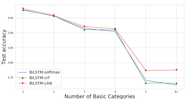
Figure 5: Accuracy against super category complexity.
图 5: 超类别复杂度对应的准确率。
Super category Complexity. We also measure the complexity of super categories by the number of basic categories that they contain. According to this definition, “S”, “S/NP” and “(S \NP)/NP” have complexities of 1, 2 and 3, respectively. Figure 5 shows the accuracy of BiLSTM-softmax, BiLSTM-CRF and BiLSTM-LAN against the supertag complexity. As the complexity increases, the performance of all the models decrease, which conforms to intuition. BiLSTM-CRF does not show obvious advantages over BiLSTM-softmax on complex categories. In contrast, BiLSTMLAN outperforms both models on complex categories, demonstrating its advantage in capturing more sophisticated label dependencies.
超级类别复杂度。我们还通过超级类别包含的基础类别数量来衡量其复杂度。根据此定义,"S"、"S/NP"和"(S \NP)/NP"的复杂度分别为1、2和3。图5展示了BiLSTM-softmax、BiLSTM-CRF和BiLSTM-LAN针对超级标签复杂度的准确率。随着复杂度增加,所有模型性能均下降,这与直觉一致。在复杂类别上,BiLSTM-CRF相比BiLSTM-softmax未显现明显优势。相比之下,BiLSTM-LAN在复杂类别上优于两者,展现出其捕捉更复杂标签依赖关系的优势。
Case Study. Some predictions of BiLSTMsoftmax, BiLSTM-CRF and BiLSTM-LAN are shown in Table 10. The sentence contains two prepositional phrases “with ...” and “at ...”, thus exemplifies the PP-attachment problem, one of the hardest sub-problems in CCG super tagging. As can be seen, BiLSTM-softmax fails to learn the long-range relation between “settled” and “at”. BiLSTM-CRF strictly follows the hard constraint between neighbor categories thanks to Markov label transition. However, it predicts “with” incorrectly as “PP/NP” with the former supertag ending with $\mathrm{^{66}/P P^{\prime}}$ . In contrast, BiLSTM-LAN can capture potential long-term dependency and better determine the supertags based on global label information. In this case, our model can effectively represent a full label search space without making Markov assumptions.
案例分析。表10展示了BiLSTMsoftmax、BiLSTM-CRF和BiLSTM-LAN的部分预测结果。该句子包含两个介词短语"with..."和"at...",体现了PP附着问题(CCG超标注中最困难的子问题之一)。可以看出,BiLSTM-softmax未能学习到"settled"与"at"之间的长距离关系。得益于马尔可夫标签转移机制,BiLSTM-CRF严格遵守相邻类别间的硬约束,但错误地将"with"预测为以$\mathrm{^{66}/P P^{\prime}}$结尾的"PP/NP"。相比之下,BiLSTM-LAN能够捕捉潜在的长程依赖,并基于全局标签信息更准确地确定超标注。本案例中,我们的模型无需马尔可夫假设即可有效表征完整的标签搜索空间。
7 Conclusion
7 结论
We investigate a hierarchically-refined label attention network (LAN) for sequence labeling, which leverages label embeddings and captures potential long-range label dependencies by deep attention al encoding of label distribution sequences. Both in theory and empirical results prove that BiLSTMLAN effective solve label bias issue. Results on POS tagging, NER and CCG super tagging show that BiLSTM-LAN outperforms BiLSTMCRF and BiLSTM-softmax.
我们研究了一种用于序列标注的分层细化标签注意力网络(LAN),该网络利用标签嵌入并通过深度注意力编码标签分布序列来捕捉潜在的远程标签依赖关系。理论和实验结果均证明,BiLSTM-LAN能有效解决标签偏差问题。在词性标注(POS)、命名实体识别(NER)和组合范畴语法(CCG)超级标注任务上的结果表明,BiLSTM-LAN优于BiLSTM-CRF和BiLSTM-softmax。
Acknowledgments
致谢
We thank Zhiyang Teng and Junchi Zhang for insightful discussions. We thank Chenhua Chen for proofreading the paper. We also thank all anonymous reviewers for their constructive comments. This work is supported by National Science Foundation of China (Grant No. 61976180). The corresponding author is Yue Zhang.
感谢滕志阳和张俊驰富有洞察力的讨论。感谢陈晨华对论文的校对。同时感谢所有匿名评审人提出的建设性意见。本研究得到中国国家自然科学基金(资助号: 61976180)的支持。通讯作者为Yue Zhang。
References
参考文献
Rami Al-Rfou, Bryan Perozzi, and Steven Skiena. 2013. Polyglot: Distributed word representations for multilingual nlp. In Proceedings of the Seventeenth Conference on Computational Natural Language Learning, pages 183–192, Sofia, Bulgaria. Association for Computational Linguistics.
Rami Al-Rfou、Bryan Perozzi和Steven Skiena。2013. Polyglot:面向多语言NLP的分布式词表示。载于《第十七届计算自然语言学习会议论文集》,第183-192页,保加利亚索菲亚。计算语言学协会。
Dzmitry Bahdanau, Kyunghyun Cho, and Yoshua Bengio. 2014. Neural machine translation by jointly learning to align and translate. arXiv preprint arXiv:1409.0473.
Dzmitry Bahdanau、Kyunghyun Cho 和 Yoshua Bengio。2014。通过联合学习对齐和翻译的神经机器翻译。arXiv 预印本 arXiv:1409.0473。
Peng Chen, Zhongqian Sun, Lidong Bing, and Wei Yang. 2017. Recurrent attention network on memory for aspect sentiment analysis. In Proceedings of the 2017 Conference on Empirical Methods in Natural Language Processing, pages 452–461. Association for Computational Linguistics.
彭晨, 孙忠谦, 宾利东, 杨威. 2017. 基于记忆循环注意力网络的方面情感分析. 载于《2017年自然语言处理实证方法会议论文集》, 第452-461页. 计算语言学协会.
Jason P.C. Chiu and Eric Nichols. 2016. Named entity recognition with bidirectional LSTM-CNNs. Transactions of the Association for Computational Linguistics, 4:357–370.
Jason P.C. Chiu 和 Eric Nichols. 2016. 基于双向LSTM-CNN的命名实体识别. Transactions of the Association for Computational Linguistics, 4:357–370.
Kevin Clark, Minh-Thang Luong, Christopher D. Manning, and Quoc Le. 2018. Semi-supervised sequence modeling with cross-view training. In Proceedings of the 2018 Conference on Empirical Methods in Natural Language Processing, pages 1914– 1925, Brussels, Belgium. Association for Computational Linguistics.
Kevin Clark、Minh-Thang Luong、Christopher D. Manning 和 Quoc Le。2018。基于交叉视角训练的半监督序列建模。载于《2018年自然语言处理实证方法会议论文集》,第1914–1925页,比利时布鲁塞尔。计算语言学协会。
Cicero Nogueira Dos Santos and Bianca Zadrozny. 2014. Learning character-level representations for part-of-speech tagging. In Proceedings of the 31st International Conference on International Conference on Machine Learning - Volume 32, ICML’14, pages II–1818–II–1826. JMLR.org.
Cicero Nogueira Dos Santos和Bianca Zadrozny。2014。学习字符级表示用于词性标注。见《第31届国际机器学习会议论文集》第32卷,ICML'14,第II-1818至II-1826页。JMLR.org。
Timothy Dozat and Christopher D Manning. 2016. Deep biaffine attention for neural dependency parsing. arXiv preprint arXiv:1611.01734.
Timothy Dozat 和 Christopher D Manning. 2016. 神经依存解析的深度双仿射注意力机制. arXiv 预印本 arXiv:1611.01734.
Greg Durrett and Dan Klein. 2014. A joint model for entity analysis: Co reference, typing, and linking. Transactions of the Association for Computational Linguistics, 2:477–490.
Greg Durrett 和 Dan Klein. 2014. 实体分析的联合模型: 共指消解、类型识别与链接. Transactions of the Association for Computational Linguistics, 2:477–490.
Abbas Ghaddar and Phillippe Langlais. 2018. Robust lexical features for improved neural network namedentity recognition. In Proceedings of the 27th International Conference on Computational Linguistics, pages 1896–1907, Santa Fe, New Mexico, USA. Association for Computational Linguistics.
Abbas Ghaddar和Phillippe Langlais。2018。用于改进神经网络命名实体识别的鲁棒词汇特征。载于《第27届国际计算语言学会议论文集》,第1896-1907页,美国新墨西哥州圣达菲。计算语言学协会。
Qipeng Guo, Xipeng Qiu, Pengfei Liu, Yunfan Shao, Xiangyang Xue, and Zheng Zhang. 2019. Startransformer. In Proceedings of the 2019 Conference of the North American Chapter of the Association for Computational Linguistics: Human Language Technologies, Volume 1 (Long and Short Papers), pages 1315–1325, Minneapolis, Minnesota. Association for Computational Linguistics.
Qipeng Guo, Xipeng Qiu, Pengfei Liu, Yunfan Shao, Xiangyang Xue, and Zheng Zhang. 2019. StarTransformer. 见《2019年北美计算语言学协会人类语言技术会议论文集(长论文与短论文)》第1卷,第1315-1325页,明尼苏达州明尼阿波利斯市。计算语言学协会。
Karl Moritz Hermann, Tomas Kocisky, Edward Gre fens te tte, Lasse Espeholt, Will Kay, Mustafa Su- leyman, and Phil Blunsom. 2015. Teaching machines to read and comprehend. In Proceedings of the 28th International Conference on Neural Information Processing Systems - Volume 1, NIPS’15, pages 1693–1701, Cambridge, MA, USA. MIT Press.
Karl Moritz Hermann、Tomas Kocisky、Edward Grefenstette、Lasse Espeholt、Will Kay、Mustafa Suleyman 和 Phil Blunsom。2015. 教机器阅读和理解。见《第28届国际神经信息处理系统会议论文集 - 第1卷》,NIPS'15,第1693-1701页,美国马萨诸塞州剑桥市。MIT出版社。
Julia Hocken maier and Mark Steedman. 2007. Ccgbank: A corpus of ccg derivations and dependency structures extracted from the penn treebank. Comput. Linguist., 33(3):355–396.
Julia Hockenmaier 和 Mark Steedman。2007。CCGBank:从宾州树库中提取的CCG派生与依存结构语料库。计算语言学,33(3):355–396。
Eduard Hovy, Mitchell Marcus, Martha Palmer, Lance Ramshaw, and Ralph Weischedel. 2006. Ontonotes: The $90%$ solution. In Proceedings of the Human Language Technology Conference of the NAACL, Companion Volume: Short Papers, NAACL-Short ’06, pages 57–60, Stroud s burg, PA, USA. Association for Computational Linguistics.
Eduard Hovy、Mitchell Marcus、Martha Palmer、Lance Ramshaw和Ralph Weischedel。2006年。Ontonotes:90%的解决方案。载于《北美计算语言学协会人类语言技术会议论文集,附卷:短论文》,NAACL-Short '06,第57-60页,美国宾夕法尼亚州斯特劳兹堡。计算语言学协会。
Zhiheng Huang, Wei Xu, and Kai Yu. 2015. Bidirectional lstm-crf models for sequence tagging. CoRR, abs/1508.01991.
Zhiheng Huang, Wei Xu, and Kai Yu. 2015. 双向LSTM-CRF序列标注模型. CoRR, abs/1508.01991.
Rudolf Kadlec, Martin Schmid, Ondrej Bajgar, and Jan Klein dien st. 2016. Text understanding with the attention sum reader network. In Proceedings of the 54th Annual Meeting of the Association for Computational Linguistics (Volume 1: Long Papers), pages 908–918. Association for Computational Linguistics.
Rudolf Kadlec、Martin Schmid、Ondrej Bajgar 和 Jan Klein dien st. 2016. 基于注意力求和阅读器网络的文本理解。载于《第54届计算语言学协会年会论文集(第一卷:长论文)》,第908–918页。计算语言学协会。
Eliyahu Ki per wasser and Yoav Goldberg. 2016. Simple and accurate dependency parsing using bidirectional LSTM feature representations. TACL, 4:313– 327.
Eliyahu Kiperwasser和Yoav Goldberg。2016。使用双向LSTM特征表示的简单准确依存解析。TACL,4:313–327。
John D. Lafferty, Andrew McCallum, and Fernando C. N. Pereira. 2001. Conditional random fields: Probabilistic models for segmenting and labeling sequence data. In Proceedings of the Eighteenth International Conference on Machine Learning, ICML ’01, pages 282–289, San Francisco, CA, USA. Mor- gan Kaufmann Publishers Inc.
John D. Lafferty、Andrew McCallum 和 Fernando C. N. Pereira。2001. 条件随机场:用于序列数据分割与标注的概率模型。在《第十八届国际机器学习会议论文集》(ICML '01) 中,第282-289页,美国加州旧金山。Morgan Kaufmann Publishers Inc.
Guillaume Lample, Miguel Ball ester os, Sandeep Subramanian, Kazuya Kawakami, and Chris Dyer. 2016. Neural architectures for named entity recognition. In Proceedings of the 2016 Conference of the North American Chapter of the Association for Computational Linguistics: Human Language Technologies, pages 260–270. Association for Computational Linguistics.
Guillaume Lample、Miguel Ballesteros、Sandeep Subramanian、Kazuya Kawakami 和 Chris Dyer。2016。命名实体识别的神经架构。载于《2016年北美计算语言学协会人类语言技术会议论文集》,第260-270页。计算语言学协会。
Mike Lewis, Kenton Lee, and Luke Z ett le moyer. 2016. Lstm ccg parsing. In Proceedings of the 2016 Conference of the North American Chapter of the Association for Computational Linguistics: Human Language Technologies, pages 221–231. Association for Computational Linguistics.
Mike Lewis、Kenton Lee 和 Luke Zettlemoyer。2016. LSTM CCG 解析。载于《2016年北美计算语言学协会人类语言技术会议论文集》,第221-231页。计算语言学协会。
Qi Li, Tianshi Li, and Baobao Chang. 2016. Discourse parsing with attention-based hierarchical neural networks. In Proceedings of the 2016 Conference on
齐力、李天石、常宝宝。2016。基于注意力机制的分层神经网络篇章解析。载于2016年会议论文集
Empirical Methods in Natural Language Processing, pages 362–371. Association for Computational Linguistics.
自然语言处理实证方法,第362-371页。计算语言学协会。
Jiangming Liu and Yue Zhang. 2017. Attention modeling for targeted sentiment. In Proceedings of the 15th Conference of the European Chapter of the Association for Computational Linguistics: Volume 2, Short Papers, pages 572–577. Association for Computational Linguistics.
Jiangming Liu 和 Yue Zhang。2017。面向目标情感分析的注意力建模。载于《第15届欧洲计算语言学协会会议论文集:第2卷,短论文》,572–577页。计算语言学协会。
Liyuan Liu, Jingbo Shang, Frank Xu, Xiang Ren, Huan Gui, Jian Peng, and Jiawei Han. 2017. Empower sequence labeling with task-aware neural language model. arXiv preprint arXiv:1709.04109.
Liyuan Liu、Jingbo Shang、Frank Xu、Xiang Ren、Huan Gui、Jian Peng和Jiawei Han。2017。基于任务感知神经语言模型的序列标注增强方法。arXiv预印本arXiv:1709.04109。
Xuezhe Ma and Eduard Hovy. 2016. End-to-end sequence labeling via bi-directional lstm-cnns-crf. In Proceedings of the 54th Annual Meeting of the Association for Computational Linguistics (Volume 1: Long Papers), pages 1064–1074. Association for Computational Linguistics.
Xuezhe Ma和Eduard Hovy。2016。基于双向LSTM-CNNs-CRF的端到端序列标注方法。载于《第54届计算语言学协会年会论文集(第一卷:长论文)》,第1064–1074页。计算语言学协会。
Christopher D. Manning. 2011. Part-of-speech tagging from $97%$ to $100%$ : Is it time for some linguistics? In Computational Linguistics and Intelligent Text Processing, pages 171–189, Berlin, Heidelberg. Springer Berlin Heidelberg.
Christopher D. Manning. 2011. 词性标注从 $97%$ 到 $100%$:是时候引入语言学了吗?载于《计算语言学与智能文本处理》,第171-189页,柏林/海德堡。Springer Berlin Heidelberg出版社。
Mitchell P. Marcus, Mary Ann Marcin kiew i cz, and Beatrice Santorini. 1993. Building a large annotated corpus of english: The penn treebank. Comput. Linguist., 19(2):313–330.
Mitchell P. Marcus, Mary Ann Marcinkiewicz 和 Beatrice Santorini. 1993. 构建大型英语标注语料库: 宾州树库 (The Penn Treebank). Comput. Linguist., 19(2):313–330.
Jinseok Nam, Eneldo Loza Mencia, and Johannes Fuirnkranz. 2016. All-in text: Learning document, label, and word representations jointly. In Proceedings of the 30th AAAI Conference on Artificial Intelligence, pages 1948–1954. AAAI Press.
Jinseok Nam、Eneldo Loza Mencia 和 Johannes Fuirnkranz。2016. 全文本学习:联合学习文档、标签和词表示。载于《第30届AAAI人工智能会议论文集》,第1948-1954页。AAAI Press。
Joakim Nivre, Mitchell Abrams, Zeljko Agic, Lars Ahrenberg, Lene Antonsen, Maria Jesus Aranz- abe, Gashaw Arutie, Masayuki Asahara, Luma Ateyah, Mohammed Attia, Aitziber Atutxa, Lies- beth Augustinus, Elena Badmaeva, Miguel Ballesteros, Esha Banerjee, Sebastian Bank, Verginica Barbu Mititelu, John Bauer, Sandra Bellato, Kepa Bengoetxea, Riyaz Ahmad Bhat, Erica Biagetti, Eckhard Bick, Rogier Blokland, Victoria Bobicev, Carl Borstell, Cristina Bosco, Gosse Bouma, Sam Bowman, Adriane Boyd, Aljoscha Burchardt, Marie Candito, Bernard Caron, Gauthier Caron, Guilsen Cebiroglu Eryigit, Giuseppe G. A. Celano, Savas Cetin, Fabricio Chalub, Jinho Choi, Yongseok Cho, Jayeol Chun, Silvie Cinkova, Aurélie Collomb, Cagri Coltekin, Miriam Connor, Marine Courtin, Elizabeth Davidson, Marie-Catherine de Marneffe, Valeria de Paiva, Arantza Diaz de Ilarraza, Carly Dickerson, Peter Dirix, Kaja Dobrovoljc, Tim- othy Dozat, Kira Droganova, Puneet Dwivedi, Marhaba Eli, Ali Elkahky, Binyam Ephrem, Tomaz Erjavec, Aline Etienne, Richard Farkas, Hector Fernandez Alcalde, Jennifer Foster, Claudia Fre- itas, Katarina Gajdosova, Daniel Galbraith, Marcos Garcia, Moa Gardenfors, Kim Gerdes, Filip
Joakim Nivre, Mitchell Abrams, Željko Agić, Lars Ahrenberg, Lene Antonsen, María Jesús Aranzabe, Gashaw Arutie, Masayuki Asahara, Luma Ateyah, Mohammed Attia, Aitziber Atutxa, Liesbeth Augustinus, Elena Badmaeva, Miguel Ballesteros, Esha Banerjee, Sebastian Bank, Verginica Barbu Mititelu, John Bauer, Sandra Bellato, Kepa Bengoetxea, Riyaz Ahmad Bhat, Erica Biagetti, Eckhard Bick, Rogier Blokland, Victoria Bobicev, Carl Borstell, Cristina Bosco, Gosse Bouma, Sam Bowman, Adriane Boyd, Aljoscha Burchardt, Marie Candito, Bernard Caron, Gauthier Caron, Gülşen Cebiroğlu Eryiğit, Giuseppe G. A. Celano, Şavas Çetin, Fabricio Chalub, Jinho Choi, Yongseok Cho, Jayeol Chun, Silvie Cinková, Aurélie Collomb, Çağrı Çöltekin, Miriam Connor, Marine Courtin, Elizabeth Davidson, Marie-Catherine de Marneffe, Valeria de Paiva, Arantza Diaz de Ilarraza, Carly Dickerson, Peter Dirix, Kaja Dobrovoljc, Timothy Dozat, Kira Droganova, Puneet Dwivedi, Marhaba Eli, Ali Elkahky, Binyam Ephrem, Tomaž Erjavec, Aline Etienne, Richárd Farkas, Héctor Fernández Alcalde, Jennifer Foster, Cláudia Freitas, Katarína Gajdošová, Daniel Galbraith, Marcos Garcia, Moa Gårdenfors, Kim Gerdes, Filip
Ginter, Iakes Goenaga, Koldo Gojenola, Memduh Gokirmak, Yoav Goldberg, Xavier Gomez Guinovart, Berta Gonzales Saavedra, Matias Grioni, Normunds Gruzitis, Bruno Guillaume, Celine Guillot- Barbance,Niza rH abash,Jan Haj,Jan Haj j, Linh Ha My, Na-Rae Han, Kim Harris, Dag Haug, Barbora Hladka, _ Jaroslava Hlavacova, Florinel Hociung, Petter Hohle, Jena Hwang, Radu Ion, Elena Irimia, Tomas Jelinek, Anders Johannsen, Fredrik Jorgensen, Huner Kasikara, Sylvain Kahane, Hiroshi Kanayama, Jenna Kanerva, Tolga Kayadelen, Vaclava Kettnerova, Jesse Kirchner, Natalia Kotsyba, Simon Krek, Sookyoung Kwak, Veronika Laippala, Lorenzo Lambertino, Tatiana Lando, Septina Dian Larasati, Alexei Lavrentiev, John Lee,Phng L Hong,Alessandro Lenci, Saran Lertpradit, Herman Leung, Cheuk Ying Li, Josie Li, Keying Li, KyungTae Lim, Nikola Ljubesic, Olga Loginova, Olga Lya she vs kaya, Teresa Lynn, Vivien Macketanz, Aibek Makazhanov, Michael Mandl, Christopher Manning, Ruli Manurung, Catalina Maranduc, David Marecek, Katrin Marhei- necke, Hector Martinez Alonso, Andre Martins, Jan Masek, Yuji Matsumoto, Ryan McDonald, Gustavo Mendonca, Niko Miekka, Anna Missila, Catalin Mititelu, Yusuke Miyao, Simonetta Montemagni, Amir More, Laura Moreno Romero, Shinsuke Mori, Bjartur Mortensen, Bohdan Mos kale vs kyi, Kadri Muischnek, Yugo Murawaki, Kaili Murisp, Pinkey Nainwani, Juan Ignacio Navarro Horniacek, Anna Nedoluzhko, Gunta Nespore-Berzkalne, Lng Nguy'én Thi, Huy'én Nguy^én Thi Minh, Vi- taly Nikolaev, Rattima Nitisaroj, Hanna Nurmi, Stina Ojala, Adédayo Oluokun, Mai Omura, Petya Osenova, Robert O¨ stling, Lilja Øvrelid, Niko Partanen, Elena Pascual, Marco Passarotti, Agnieszka Patejuk, Siyao Peng, Cenel-Augusto Perez, Guy Perrier, Slav Petrov, Jussi P ii tula inen, Emily Pitler, Barbara Plank, Thierry Poibeau, Martin Popel, Lauma Pre t kal nina, Sophie Prevost, Prokopis Prokopidis, Adam Pr zep i or ko w ski, Ti- ina Pu ola kaine n, Sampo Pyysalo, Andriela Raabis, Alexandre Rademaker, Loganathan Ramasamy, Taraka Rama, Carlos Ramisch, Vinit Ravi shankar, Livy Real, Siva Reddy, Georg Rehm, Michael Rießler, Larissa Rinaldi, Laura Rituma, Luisa Rocha, Mykhailo Romanenko, Rudolf Rosa, Davide Rovati, Valentin Roca, Olga Rudina, Shoval Sadde, Shadi Saleh, Tanja Samardzic, Stephanie Samson, Manuela Sanguinetti, Baiba Saulite, Yanin Saw an a kuna non, Nathan Schneider, Sebas- tian Schuster, Djamé Seddah, Wolfgang Seeker, Mojgan Seraji, Mo Shen, Atsuko Shimada, Muh Sho hi bus sir ri, Dmitry Sichinava, Natalia Silveira, Maria Simi, Radu Simionescu, Katalin Simko, Maria Simkova, Kiril Simov, Aaron Smith, Isabela Soares-Bastos, Antonio Stella, Milan Straka, Jana Strnadova, Alane Suhr, Umut Sulubacak, Zsolt Szanto, Dima Taji, Yuta Takahashi, Takaaki Tanaka, Isabelle Tellier, Trond Trosterud, Anna Trukhina, Reut Tsarfaty, Francis Tyers, Sumire Ue- matsu, Zdenka Uresova, Larraitz Uria, Hans Uszko- reit, Sowmya Vajjala, Daniel van Niekerk, Gertjan van Noord, Viktor Varga, Veronika Vincze, Lars Wallin, Jonathan North Washington, Seyi Williams, Mats Wirén, Tsegay Wold e mariam, Tak-sum Wong, Chunxiao Yan, Marat M. Yavrumyan, Zhuoran Yu, Zdenek Zabokrtsky, Amir Zeldes, Daniel Zeman, Manying Zhang, and Hanzhi Zhu. 2018. Universal dependencies 2.2. LINDAT/CLARIN digital library at the Institute of Formal and Applied Linguistics ( U´ FAL), Faculty of Mathematics and Physics, Charles University.
Ginter、Iakes Goenaga、Koldo Gojenola、Memduh Gokirmak、Yoav Goldberg、Xavier Gomez Guinovart、Berta Gonzales Saavedra、Matias Grioni、Normunds Gruzitis、Bruno Guillaume、Celine Guillot-Barbance、Nizar Habash、Jan Hajic、Jan Hajic jr.、Linh Ha My、Na-Rae Han、Kim Harris、Dag Haug、Barbora Hladka、Jaroslava Hlavacova、Florinel Hociung、Petter Hohle、Jena Hwang、Radu Ion、Elena Irimia、Tomas Jelinek、Anders Johannsen、Fredrik Jorgensen、Huner Kasikara、Sylvain Kahane、Hiroshi Kanayama、Jenna Kanerva、Tolga Kayadelen、Vaclava Kettnerova、Jesse Kirchner、Natalia Kotsyba、Simon Krek、Sookyoung Kwak、Veronika Laippala、Lorenzo Lambertino、Tatiana Lando、Septina Dian Larasati、Alexei Lavrentiev、John Lee、Phuong Le Hong、Alessandro Lenci、Saran Lertpradit、Herman Leung、Cheuk Ying Li、Josie Li、Keying Li、KyungTae Lim、Nikola Ljubesic、Olga Loginova、Olga Lyashevskaya、Teresa Lynn、Vivien Macketanz、Aibek Makazhanov、Michael Mandl、Christopher Manning、Ruli Manurung、Catalina Maranduc、David Marecek、Katrin Marheinecke、Hector Martinez Alonso、Andre Martins、Jan Masek、Yuji Matsumoto、Ryan McDonald、Gustavo Mendonca、Niko Miekka、Anna Missila、Catalin Mititelu、Yusuke Miyao、Simonetta Montemagni、Amir More、Laura Moreno Romero、Shinsuke Mori、Bjartur Mortensen、Bohdan Moskalevskyi、Kadri Muischnek、Yugo Murawaki、Kaili Muresp、Pinkey Nainwani、Juan Ignacio Navarro Horniacek、Anna Nedoluzhko、Gunta Nespore-Berzkalne、Linh Nguyen Thi、Huyen Nguyen Thi Minh、Vitaly Nikolaev、Rattima Nitisaroj、Hanna Nurmi、Stina Ojala、Adedayo Oluokun、Mai Omura、Petya Osenova、Robert Ostling、Lilja Ovrelid、Niko Partanen、Elena Pascual、Marco Passarotti、Agnieszka Patejuk、Siyao Peng、Cenel-Augusto Perez、Guy Perrier、Slav Petrov、Jussi Piitulainen、Emily Pitler、Barbara Plank、Thierry Poibeau、Martin Popel、Lauma Pretkalnina、Sophie Prevost、Prokopis Prokopidis、Adam Przepiorkowski、Tiina Puolakainen、Sampo Pyysalo、Andriela Raabis、Alexandre Rademaker、Loganathan Ramasamy、Taraka Rama、Carlos Ramisch、Vinit Ravishankar、Livy Real、Siva Reddy、Georg Rehm、Michael Rießler、Larissa Rinaldi、Laura Rituma、Luisa Rocha、Mykhailo Romanenko、Rudolf Rosa、Davide Rovati、Valentin Rocca、Olga Rudina、Shoval Sadde、Shadi Saleh、Tanja Samardzic、Stephanie Samson、Manuela Sanguinetti、Baiba Saulite、Yanin Sawanakunanon、Nathan Schneider、Sebastian Schuster、Djame Seddah、Wolfgang Seeker、Mojgan Seraji、Mo Shen、Atsuko Shimada、Muh Shohibussirri、Dmitry Sichinava、Natalia Silveira、Maria Simi、Radu Simionescu、Katalin Simko、Maria Simkova、Kiril Simov、Aaron Smith、Isabela Soares-Bastos、Antonio Stella、Milan Straka、Jana Strnadova、Alane Suhr、Umut Sulubacak、Zsolt Szanto、Dima Taji、Yuta Takahashi、Takaaki Tanaka、Isabelle Tellier、Trond Trosterud、Anna Trukhina、Reut Tsarfaty、Francis Tyers、Sumire Uematsu、Zdenka Uresova、Larraitz Uria、Hans Uszkoreit、Sowmya Vajjala、Daniel van Niekerk、Gertjan van Noord、Viktor Varga、Veronika Vincze、Lars Wallin、Jonathan North Washington、Seyi Williams、Mats Wiren、Tsegay Woldemariam、Tak-sum Wong、Chunxiao Yan、Marat M. Yavrumyan、Zhuoran Yu、Zdenek Zabokrtsky、Amir Zeldes、Daniel Zeman、Manying Zhang和Hanzhi Zhu。2018。通用依存关系2.2。林达特/克拉林数字图书馆,形式与应用语言学研究所(UFAL),数学与物理学院,查理大学。
Mark Palatucci, Dean Pomerleau, Geoffrey E Hinton, and Tom M Mitchell. 2009. Zero-shot learning with semantic output codes. In Y. Bengio, D. Schuurmans, J. D. Lafferty, C. K. I. Williams, and A. Culotta, editors, Advances in Neural Information Processing Systems 22, pages 1410–1418. Curran Associates, Inc.
Mark Palatucci、Dean Pomerleau、Geoffrey E Hinton 和 Tom M Mitchell。2009. 零样本学习与语义输出编码。见 Y. Bengio、D. Schuurmans、J. D. Lafferty、C. K. I. Williams 和 A. Culotta 编辑,《神经信息处理系统进展 22》,第 1410–1418 页。Curran Associates, Inc.
Fuchun Peng, Fangfang Feng, and Andrew McCallum. 2004. Chinese segmentation and new word detection using conditional random fields. In Proceedings of the 20th International Conference on Computational Linguistics, COLING $^{\ '}04$ , Stroud s burg, PA, USA. Association for Computational Linguistics.
Fuchun Peng、Fangfang Feng 和 Andrew McCallum。2004。基于条件随机场 (Conditional Random Fields) 的中文分词与新词检测。载于《第20届国际计算语言学会议论文集》(COLING '04) ,美国宾夕法尼亚州斯特劳斯堡。计算语言学协会。
Jeffrey Pennington, Richard Socher, and Christopher D. Manning. 2014. Glove: Global vectors for word representation. In Empirical Methods in Natural Language Processing (EMNLP), pages 1532– 1543.
Jeffrey Pennington、Richard Socher 和 Christopher D. Manning. 2014. Glove: 全局词向量表示. 载于《自然语言处理实证方法》(EMNLP), 第1532–1543页.
Barbara Plank, Anders Søgaard, and Yoav Goldberg. 2016. Multilingual part-of-speech tagging with bidirectional long short-term memory models and auxiliary loss. In Proceedings of the 54th Annual Meeting of the Association for Computational Linguistics (Volume 2: Short Papers), pages 412–418. Association for Computational Linguistics.
Barbara Plank、Anders Søgaard和Yoav Goldberg。2016。基于双向长短期记忆模型和辅助损失的多语言词性标注。载于《第54届计算语言学协会年会论文集(第二卷:短论文)》,第412-418页。计算语言学协会。
Sameer Pradhan, Alessandro Moschitti, Nianwen Xue, Hwee Tou Ng, Anders Bjorkelund, Olga Uryupina, Yuchen Zhang, and Zhi Zhong. 2013. Towards robust linguistic analysis using OntoNotes. In Proceedings of the Seventeenth Conference on Computational Natural Language Learning, pages 143– 152, Sofia, Bulgaria. Association for Computational Linguistics.
Sameer Pradhan、Alessandro Moschitti、Nianwen Xue、Hwee Tou Ng、Anders Bjorkelund、Olga Uryupina、Yuchen Zhang 和 Zhi Zhong。2013. 基于 OntoNotes 的鲁棒语言分析研究。载于《第十七届计算自然语言学习会议论文集》,第143-152页,保加利亚索菲亚。计算语言学协会。
Sameer Pradhan, Alessandro Moschitti, Nianwen Xue, Olga Uryupina, and Yuchen Zhang. 2012. CoNLL2012 shared task: Modeling multilingual unrestricted co reference in OntoNotes. In Joint Conference on EMNLP and CoNLL - Shared Task, pages 1–40, Jeju Island, Korea. Association for Computational Linguistics.
Sameer Pradhan、Alessandro Moschitti、Nianwen Xue、Olga Uryupina 和 Yuchen Zhang。2012. CoNLL2012 共享任务:在 OntoNotes 中建模多语言无限制共指消解。载于 EMNLP 和 CoNLL 联合会议 - 共享任务,第 1-40 页,韩国济州岛。计算语言学协会。
Lev Ratinov and Dan Roth. 2009. Design challenges and misconceptions in named entity recognition. In Proceedings of the Thirteenth Conference on Computational Natural Language Learning, CoNLL ’09, pages 147–155, Stroud s burg, PA, USA. Association for Computational Linguistics.
Lev Ratinov 和 Dan Roth. 2009. 命名实体识别中的设计挑战与误解. 载于《第十三届计算自然语言学习会议论文集》(CoNLL '09), 第147-155页, 美国宾夕法尼亚州斯特劳兹堡. 计算语言学协会.
Nils Reimers and Iryna Gurevych. 2017. Optimal hyper parameters for deep lstm-networks for sequence labeling tasks. arXiv preprint arXiv:1707.06799.
Nils Reimers 和 Iryna Gurevych。2017。序列标注任务中深度 LSTM 网络的最优超参数 (Optimal hyper parameters for deep lstm-networks for sequence labeling tasks)。arXiv 预印本 arXiv:1707.06799。
Alexander M. Rush, Sumit Chopra, and Jason Weston. 2015. A neural attention model for abstract ive sentence sum mari z ation. In Proceedings of the 2015 Conference on Empirical Methods in Natural Language Processing, pages 379–389. Association for Computational Linguistics.
Alexander M. Rush、Sumit Chopra 和 Jason Weston。2015。基于神经注意力模型的抽象式句子摘要生成。载于《2015年自然语言处理实证方法会议论文集》,第379-389页。计算语言学协会。
Yanyao Shen, Hyokun Yun, Zachary Lipton, Yakov Kronrod, and Animashree Anandkumar. 2017. Deep active learning for named entity recognition. In Proceedings of the 2nd Workshop on Representation Learning for NLP, pages 252–256, Vancouver, Canada. Association for Computational Linguistics.
Yanyao Shen、Hyokun Yun、Zachary Lipton、Yakov Kronrod 和 Animashree Anandkumar。2017. 命名实体识别的深度主动学习。载于《第二届自然语言处理表征学习研讨会论文集》,第252-256页,加拿大温哥华。计算语言学协会。
Natalia Silveira, Timothy Dozat, Marie-Catherine de Marneffe, Samuel Bowman, Miriam Connor, John Bauer, and Christopher D. Manning. 2014. A gold standard dependency corpus for English. In Proceedings of the Ninth International Conference on Language Resources and Evaluation (LREC2014).
Natalia Silveira、Timothy Dozat、Marie-Catherine de Marneffe、Samuel Bowman、Miriam Connor、John Bauer和Christopher D. Manning。2014. 英语依存关系标注的黄金标准语料库。载于《第九届国际语言资源与评估会议论文集》(LREC2014)。
Richard Socher, Milind Ganjoo, Christopher D. Manning, and Andrew Y. Ng. 2013. Zero-shot learning through cross-modal transfer. In Proceedings of the 26th International Conference on Neural Information Processing Systems - Volume 1, NIPS’13, pages 935–943, USA. Curran Associates Inc.
Richard Socher、Milind Ganjoo、Christopher D. Manning 和 Andrew Y. Ng. 2013. 通过跨模态迁移实现零样本学习 (Zero-shot Learning). 发表于《第26届国际神经信息处理系统会议论文集》第1卷, NIPS'13, 第935–943页, 美国. Curran Associates Inc.
Anders Søgaard and Yoav Goldberg. 2016. Deep multi-task learning with low level tasks supervised at lower layers. In Proceedings of the 54th Annual Meeting of the Association for Computational Linguistics (Volume 2: Short Papers), pages 231–235. Association for Computational Linguistics.
Anders Søgaard 和 Yoav Goldberg. 2016. 基于底层监督的深度多任务学习. 见《第54届计算语言学协会年会论文集(第二卷: 短论文)》, 第231-235页. 计算语言学协会.
Emma Strubell, Patrick Verga, Daniel Andor, David Weiss, and Andrew McCallum. 2018. Linguistically-informed self-attention for semantic role labeling. In Proceedings of the 2018 Conference on Empirical Methods in Natural Language Processing, pages 5027–5038. Association for Computational Linguistics.
Emma Strubell、Patrick Verga、Daniel Andor、David Weiss 和 Andrew McCallum。2018. 基于语言学信息的自注意力机制在语义角色标注中的应用。载于《2018年自然语言处理实证方法会议论文集》,第5027-5038页。计算语言学协会。
Emma Strubell, Patrick Verga, David Belanger, and Andrew McCallum. 2017. Fast and accurate entity recognition with iterated dilated convolutions. In Proceedings of the 2017 Conference on Empirical Methods in Natural Language Processing, pages 2670–2680, Copenhagen, Denmark. Association for Computational Linguistics.
Emma Strubell、Patrick Verga、David Belanger 和 Andrew McCallum。2017. 使用迭代扩张卷积实现快速准确的实体识别。载于《2017年自然语言处理实证方法会议论文集》,第2670–2680页,丹麦哥本哈根。计算语言学协会。
Jian Tang, Meng Qu, and Qiaozhu Mei. 2015. Pte: Predictive text embedding through large-scale heterogeneous text networks. In Proceedings of the 21th ACM SIGKDD International Conference on Knowledge Discovery and Data Mining, pages 1165–1174. ACM.
Jian Tang、Meng Qu和Qiaozhu Mei。2015。PTE:通过大规模异构文本网络进行预测性文本嵌入。见《第21届ACM SIGKDD知识发现与数据挖掘国际会议论文集》,第1165-1174页。ACM。
Zhiyang Teng and Yue Zhang. 2018. Two local models for neural constituent parsing. In Proceedings of the 27th International Conference on Computational Linguistics, pages 119–132. Association for Computational Linguistics.
Zhiyang Teng和Yue Zhang。2018。两种用于神经成分解析的局部模型。载于《第27届国际计算语言学会议论文集》,第119-132页。计算语言学协会。
Kristina Toutanova, Dan Klein, Christopher D. Man- ning, and Yoram Singer. 2003. Feature-rich part-ofspeech tagging with a cyclic dependency network. In Proceedings of the 2003 Conference of the North American Chapter of the Association for Computational Linguistics on Human Language Technology - Volume 1, NAACL $^{\ '}03$ , pages 173–180, Stroudsburg, PA, USA. Association for Computational Linguistics.
Kristina Toutanova、Dan Klein、Christopher D. Manning 和 Yoram Singer。2003. 基于循环依赖网络的特征丰富词性标注方法。载于《北美计算语言学协会2003年人类语言技术会议论文集》第1卷 (NAACL '03) ,第173-180页,美国宾夕法尼亚州斯特劳兹堡。计算语言学协会。
Lifu Tu and Kevin Gimpel. 2018. Learning approximate inference networks for structured prediction. In Proceedings of International Conference on Learning Representations (ICLR).
Lifu Tu 和 Kevin Gimpel. 2018. 结构化预测的近似推理网络学习. 见《国际学习表征会议论文集》(ICLR).
Lifu Tu and Kevin Gimpel. 2019. Benchmarking approximate inference methods for neural structured prediction. In Proceedings of the 2019 Conference of the North American Chapter of the Association for Computational Linguistics: Human Language Technologies, Volume 1 (Long and Short Papers), pages 3313–3324, Minneapolis, Minnesota. Association for Computational Linguistics.
Lifu Tu和Kevin Gimpel。2019。神经结构化预测中近似推理方法的基准测试。载于《2019年北美计算语言学协会人类语言技术会议论文集》第1卷(长文与短文),第3313–3324页,明尼苏达州明尼阿波利斯市。计算语言学协会。
A. Vaswani, Y. Bisk, K. Sagae, and R. Musa. 2016a. Super tagging with LSTMs. In Proc. NAACL.
A. Vaswani, Y. Bisk, K. Sagae, and R. Musa. 2016a. 基于LSTM的超级标注。见Proc. NAACL。
Ashish Vaswani, Yonatan Bisk, Kenji Sagae, and Ryan Musa. 2016b. Super tagging with lstms. In Proceedings of the 2016 Conference of the North American Chapter of the Association for Computational Linguistics: Human Language Technologies, pages 232–237. Association for Computational Linguistics.
Ashish Vaswani、Yonatan Bisk、Kenji Sagae和Ryan Musa。2016b。基于LSTM的超级标注。载于《2016年北美计算语言学协会人类语言技术会议论文集》第232-237页。计算语言学协会。
Ashish Vaswani, Noam Shazeer, Niki Parmar, Jakob Uszkoreit, Llion Jones, Aidan N Gomez, Ł ukasz Kaiser, and Illia Polosukhin. 2017. Attention is all you need. In I. Guyon, U. V. Luxburg, S. Bengio, H. Wallach, R. Fergus, S. Vishwanath an, and R. Garnett, editors, Advances in Neural Information Processing Systems 30, pages 5998–6008. Curran Associates, Inc.
Ashish Vaswani、Noam Shazeer、Niki Parmar、Jakob Uszkoreit、Llion Jones、Aidan N Gomez、Łukasz Kaiser 和 Illia Polosukhin。2017. Attention is all you need。收录于 I. Guyon、U. V. Luxburg、S. Bengio、H. Wallach、R. Fergus、S. Vishwanathan 和 R. Garnett 编辑的《Advances in Neural Information Processing Systems 30》,第5998-6008页。Curran Associates公司出版。
Guoyin Wang, Chunyuan Li, Wenlin Wang, Yizhe Zhang, Dinghan Shen, Xinyuan Zhang, Ricardo Henao, and Lawrence Carin. 2018a. Joint em- bedding of words and labels for text classification. arXiv preprint arXiv:1805.04174.
Guoyin Wang、Chunyan Li、Wenlin Wang、Yizhe Zhang、Dinghan Shen、Xinyuan Zhang、Ricardo Henao 和 Lawrence Carin。2018a。面向文本分类的词与标签联合嵌入方法。arXiv预印本 arXiv:1805.04174。
Lu Wang, Shoushan Li, Changlong Sun, Luo Si, Xiaozhong Liu, Min Zhang, and Guodong Zhou. 2018b. One vs. many qa matching with both wordlevel and sentence-level attention network. In Proceedings of the 27th International Conference on Computational Linguistics, pages 2540–2550. Association for Computational Linguistics.
Lu Wang、Shoushan Li、Changlong Sun、Luo Si、Xiaozhong Liu、Min Zhang和Guodong Zhou。2018b。基于词级与句级注意力网络的一对多问答匹配。载于《第27届国际计算语言学会议论文集》,第2540–2550页。计算语言学协会。
Xun Wang, Katsuhito Sudoh, and Masaaki Nagata. 2015. Empty category detection with joint contextlabel embeddings. In Proceedings of the 2015 Conference of the North American Chapter of the Association for Computational Linguistics: Human Language Technologies, pages 263–271. Association for Computational Linguistics.
王迅、Katsuhito Sudoh和长田正明。2015. 基于联合上下文标签嵌入的空范畴检测。载于《2015年北美计算语言学协会人类语言技术会议论文集》,第263-271页。计算语言学协会。
Wei Wu, Houfeng Wang, Tianyu Liu, and Shuming Ma. 2018. Phrase-level self-attention networks for universal sentence encoding. In Proceedings of the 2018 Conference on Empirical Methods in Natural Language Processing, pages 3729–3738. Association for Computational Linguistics.
Wei Wu、Houfeng Wang、Tianyu Liu和Shuming Ma。2018。面向通用句子编码的短语级自注意力网络。载于《2018年自然语言处理实证方法会议论文集》,第3729-3738页。计算语言学协会。
Yingwei Xin, Ethan Hart, Vibhuti Mahajan, and JeanDavid Ruvini. 2018. Learning better internal structure of words for sequence labeling. In Proceedings of the 2018 Conference on Empirical Methods in Natural Language Processing, pages 2584–2593, Brussels, Belgium. Association for Computational Linguistics.
应伟新、Ethan Hart、Vibhuti Mahajan和JeanDavid Ruvini。2018。学习更好的词内部结构以用于序列标注。载于《2018年自然语言处理经验方法会议论文集》,第2584–2593页,比利时布鲁塞尔。计算语言学协会。
Chang Xu, Cecile Paris, Surya Nepal, and Ross Sparks. 2018. Cross-target stance classification with selfattention networks. In Proceedings of the 56th Annual Meeting of the Association for Computational Linguistics (Volume 2: Short Papers), pages 778– 783. Association for Computational Linguistics.
常旭、Cecile Paris、Surya Nepal和Ross Sparks。2018。基于自注意力网络的跨目标立场分类。载于《第56届计算语言学协会年会论文集(第二卷:短论文)》,第778-783页。计算语言学协会。
Wenduan Xu, Michael Auli, and Stephen Clark. 2015. Ccg super tagging with a recurrent neural network. In Proceedings of the 53rd Annual Meeting of the Association for Computational Linguistics and the 7th International Joint Conference on Natural Language Processing (Volume 2: Short Papers), pages 250–255. Association for Computational Linguistics.
Wenduan Xu、Michael Auli 和 Stephen Clark。2015。基于循环神经网络的CCG超标注。载于《第53届计算语言学协会年会暨第7届自然语言处理国际联合会议论文集(第二卷:短论文)》,第250-255页。计算语言学协会。
Jie Yang, Shuailong Liang, and Yue Zhang. 2018. Design challenges and misconceptions in neural sequence labeling. In Proceedings of the 27th International Conference on Computational Linguistics (COLING).
Jie Yang、Shuailong Liang和Yue Zhang。2018。神经序列标注的设计挑战与误解。载于第27届国际计算语言学会议(COLING)论文集。
Jie Yang and Yue Zhang. 2018. Ncrf+ $^+$ : An opensource neural sequence labeling toolkit. In Proceedings of the 56th Annual Meeting of the Association for Computational Linguistics.
Jie Yang和Yue Zhang。2018。NCRF++:一个开源的神经序列标注工具包。见《第56届计算语言学协会年会论文集》。
Michihiro Yasunaga, Jungo Kasai, and Dragomir Radev. 2018. Robust multilingual part-of-speech tagging via adversarial training. In Proceedings of the 2018 Conference of the North American Chapter of the Association for Computational Linguistics: Human Language Technologies, Volume 1 (Long Papers), pages 976–986. Association for Computational Linguistics.
Michihiro Yasunaga、Jungo Kasai和Dragomir Radev。2018。基于对抗训练的鲁棒多语言词性标注。载于《2018年北美计算语言学协会人类语言技术会议论文集》第1卷(长论文),第976–986页。计算语言学协会。
Honglun Zhang, Liqiang Xiao, Wenqing Chen, Yongkun Wang, and Yaohui Jin. 2018a. Multi-task label embedding for text classification. In Proceedings of the 2018 Conference on Empirical Methods in Natural Language Processing, pages 4545–4553. Association for Computational Linguistics.
Honglun Zhang、Liqiang Xiao、Wenqing Chen、Yongkun Wang 和 Yaohui Jin。2018a。面向文本分类的多任务标签嵌入。载于《2018年自然语言处理实证方法会议论文集》,第4545–4553页。计算语言学协会。
Yuan Zhang, Hongshen Chen, Yihong Zhao, Qun Liu, and Dawei Yin. 2018b. Learning tag dependencies for sequence tagging. In Proceedings of the TwentySeventh International Joint Conference on Artificial Intelligence, IJCAI-18, pages 4581–4587. International Joint Conferences on Artificial Intelligence Organization.
Yuan Zhang, Hongshen Chen, Yihong Zhao, Qun Liu, and Dawei Yin. 2018b. 学习序列标注中的标签依赖关系。在《第二十七届国际人工智能联合会议论文集》(IJCAI-18)中,第4581-4587页。国际人工智能联合会议组织。
Yue Zhang, Qi Liu, and Linfeng Song. 2018c. Sentence-state lstm for text representation. In Proceedings of the 56th Annual Meeting of the Association for Computational Linguistics (Volume 1: Long Papers), pages 317–327. Association for Computational Linguistics.
Yue Zhang、Qi Liu和Linfeng Song。2018c。用于文本表示的句子状态LSTM。载于《第56届计算语言学协会年会论文集(第一卷:长论文)》,第317–327页。计算语言学协会。
Z. Zhang and V. Saligrama. 2016. Zero-shot learning via joint latent similarity embedding. In 2016 IEEE Conference on Computer Vision and Pattern Recognition (CVPR), pages 6034–6042.
Z. Zhang 和 V. Saligrama. 2016. 基于联合潜在相似性嵌入的零样本学习. 见: 2016 IEEE 计算机视觉与模式识别会议 (CVPR), 第 6034–6042 页.
Jie Zhou and Wei Xu. 2015. End-to-end learning of semantic role labeling using recurrent neural networks. In Proceedings of the 53rd Annual Meeting of the Association for Computational Linguis- tics and the 7th International Joint Conference on Natural Language Processing (Volume 1: Long Papers), pages 1127–1137. Association for Computational Linguistics.
周杰和徐伟。2015。使用循环神经网络端到端学习语义角色标注。见《第53届计算语言学协会年会暨第7届自然语言处理国际联合会议论文集(第一卷:长论文)》,第1127-1137页。计算语言学协会。
Peng Zhou, Wei Shi, Jun Tian, Zhenyu Qi, Bingchen Li, Hongwei Hao, and Bo Xu. 2016. Attentionbased bidirectional long short-term memory networks for relation classification. In Proceedings of the 54th Annual Meeting of the Association for Computational Linguistics (Volume 2: Short Papers), pages 207–212. Association for Computational Linguistics.
彭周, 魏石, 田俊, 齐振宇, 李炳辰, 郝宏伟, 徐波. 2016. 基于注意力机制的双向长短期记忆网络在关系分类中的应用. 见: 第54届计算语言学协会年会论文集 (第二卷: 短论文), 207–212页. 计算语言学协会.
Appendices
附录
A Hyper-Parameters
超参数
Table 11: Hyper-parameters.
表 11: 超参数。
| 超参数 | 值 |
|---|---|
| 字符嵌入 | 30 |
| 字符级隐藏大小 | 50 |
| 词级隐藏大小 (英语) | 400 |
| 词级隐藏大小 (其他语言) | 200 |
| 编码器层数 (POS) | 3 |
| 编码器层数 (NER) | 4 |
| 编码器层数 (CCG) | 5 |
| 注意力头数量 | 5 |
| 丢弃率 | 0.5 |
| 批量大小 | 10 |
| 优化器 | SGD |
| 动量 | 0.9 |
| L2正则化 | 1e-8 |
| 学习率 | 0.01 |
| 衰减率 (POS) | 0.035 |
| 衰减率 (NER) | 0.04 |
| 衰减率 (CCG) | 0.05 |
| 5.0 |
Tabel 11 shows the hyper-parameters of BiLSTM-LAN used for all the experiments in the papers.
表 11: 展示了论文中所有实验使用的 BiLSTM-LAN 超参数。
B Attention Visualization
B 注意力可视化

Figure 6: Attention visualization s for first and last attention layer, respectively. The color depth expresses the word’s preference degree for each label in attention vector.
图 6: 分别展示第一层和最后一层注意力层的可视化效果。颜色深度表示注意力向量中每个标签对应的词语偏好程度。
Here we continue the analysis of visualization from Section 6, we also visualize the label attention weights of BiLSTM-LAN, given the sentence in “Tell (VB) us (PRP) about (IN) spending (NN) restraint (NN)”. As shown in Figure 6, the first layer contains initial label distributions according to unigram information, in which much ambiguity remains. For example, likely POS tags for the word “spending” include “JJ”, “NN”, “VBG”, “TO” and “RBS”, while the attention layer assigns some probabilities to almost every label. In the second layer, the label distribution of every word becomes sharp and concentrated on the most probable tags in the sentential context. Here the word “spending” bares only “NN” and “VBG” labels, with relatively more probability (0.114) being assigned to “NN”.
我们延续第6节的可视化分析,针对句子"Tell (VB) us (PRP) about (IN) spending (NN) restraint (NN)"展示了BiLSTM-LAN的标签注意力权重可视化结果。如图6所示,第一层包含基于单字信息的初始标签分布,其中仍存在大量歧义。例如单词"spending"可能对应的词性标签包括"JJ"、"NN"、"VBG"、"TO"和"RBS",而注意力层几乎为每个标签都分配了概率值。在第二层中,每个单词的标签分布变得尖锐,并集中在句子上下文中最可能的标签上。此时单词"spending"仅保留"NN"和"VBG"标签,其中"NN"标签获得了相对更高的概率值(0.114)。