Deep Constrained Least Squares for Blind Image Super-Resolution
基于深度约束最小二乘的盲图像超分辨率重建
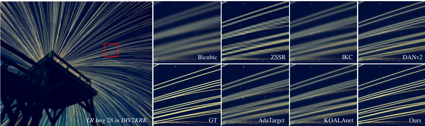
Figure 1. Blind super-resolution of Img 28 from DIV2KRK [3], for scale factor 4. Based on the proposed deep constrained least squares (DCLS) de convolution, our method is effective in restoring sharp and clean edges, and outperforms previous state-of-the-art approaches such as KernelGAN $[3]+Z S S\mathrm{\textperthousand}$ [41], IKC [9], DAN [30, 31], AdaTarget [14], and KOALAnet [19].
图 1: 基于DIV2KRK [3]数据集中Img 28的盲超分辨率重建(放大因子4)。通过提出的深度约束最小二乘(DCLS)反卷积方法,我们的方案能有效恢复清晰锐利的边缘,其性能优于KernelGAN $[3]+Z S S\mathrm{\textperthousand}$ [41]、IKC [9]、DAN [30, 31]、AdaTarget [14]和KOALAnet [19]等现有最优方法。
Abstract
摘要
In this paper, we tackle the problem of blind image superresolution(SR) with a reformulated degradation model and two novel modules. Following the common practices of blind SR, our method proposes to improve both the kernel estimation as well as the kernel based high resolution image restoration. To be more specific, we first reformulate the degradation model such that the deblurring kernel estimation can be transferred into the low resolution space. On top of this, we introduce a dynamic deep linear filter module. Instead of learning a fixed kernel for all images, it can adaptively generate deblurring kernel weights conditional on the input and yields more robust kernel estimation. Subsequently, a deep constrained least square filtering module is applied to generate clean features based on the reformulation and estimated kernel. The deblurred feature and the low input image feature are then fed into a dual-path structured SR network and restore the final high resolution result. To evaluate our method, we further conduct evaluations on several benchmarks, including Gaussian8 and DIV2KRK. Our experiments demonstrate that the proposed method achieves better accuracy and visual improvements against state-of-the-art methods.
本文通过重新构建退化模型和引入两个新模块,解决了盲图像超分辨率(SR)问题。遵循盲SR的常规做法,我们的方法旨在改进核估计以及基于核的高分辨率图像恢复。具体而言,我们首先重构退化模型,使得去模糊核估计可以转换到低分辨率空间。在此基础上,我们提出了动态深度线性滤波模块,该模块能够根据输入自适应生成去模糊核权重,而非为所有图像学习固定核,从而获得更稳健的核估计。随后,应用深度约束最小二乘滤波模块,基于重构模型和估计核生成清晰特征。去模糊特征与低分辨率输入图像特征随后被送入双路径结构的SR网络,最终恢复出高分辨率结果。为评估方法性能,我们在Gaussian8和DIV2KRK等多个基准测试上进行了实验验证。结果表明,所提方法在精度和视觉效果上均优于当前最优方法。
1. Introduction
1. 引言
In this work, we study the problem of image superresolution,i.e., restoring high-resolution images from lowresolution inputs. Specially, we aim for single image superresolution (SISR), where only one observation is given which is a more practical setting and with a wide range of downstream applications [6, 8, 10, 17, 22, 26, 28, 48, 57, 59].
在本工作中,我们研究图像超分辨率问题,即从低分辨率输入恢复高分辨率图像。特别地,我们专注于单图像超分辨率 (SISR),其中仅给定一个观测值,这是一种更实用的设置,并具有广泛的下游应用 [6, 8, 10, 17, 22, 26, 28, 48, 57, 59]。
Most existing works based on the classical SISR degradation model assuming that the input LR image $\mathbf{y}$ is a blurred and down-scaled HR image $\mathbf{x}$ with additional white Gaussian noise $\mathbf{n}$ , given by
大多数现有工作基于经典的SISR(单图像超分辨率)退化模型,假设输入的低分辨率(LR)图像$\mathbf{y}$是由高分辨率(HR)图像$\mathbf{x}$经过模糊和下采样后叠加高斯白噪声$\mathbf{n}$得到的,其表达式为
$$
\mathbf{y}=(\mathbf{x}*\mathbf{k}{h})_{\downarrow s}+\mathbf{n},
$$
$$
\mathbf{y}=(\mathbf{x}*\mathbf{k}{h})_{\downarrow s}+\mathbf{n},
$$
where $\mathbf{k}{h}$ is the blur kernel applied on $\mathbf{x},*$ denotes convolution operation and $\downarrow_{s}$ denotes down sampling with scale fac- tor $s$ . Previous blind SR approaches [9, 30] generally solve this problem with a two-stage framework: kernel estimation from LR image and kernel based HR image restoration.
其中 $\mathbf{k}{h}$ 是应用于 $\mathbf{x}$ 的模糊核,$*$ 表示卷积操作,$\downarrow_{s}$ 表示尺度因子为 $s$ 的下采样。以往的盲超分辨率方法 [9, 30] 通常采用两阶段框架解决该问题:从低分辨率图像估计核,以及基于核的高分辨率图像恢复。
We argue that although such a pipeline demonstrates reasonable performance for SR problem, there are two main drawbacks: First of all, it is difficult to accurately estimate blur kernels of HR space directly from LR images due to the ambiguity produced by under sampling step [38, 46]. And the mismatch between the estimated kernel and the real one will cause significant performance drop and even lead to unpleasant artifacts [3, 9, 13, 56]. Secondly, it is also challenging to find a suitable way to fully utilize the information of the estimated HR space kernel and LR space image. A common solution is to employ a kernel stretching strategy [9,30,56], where the principal components of the vectorized kernel are preserved and stretched into degradation maps with the same size as the LR input. These degradation maps then can be concatenated with the input image or its features to generate a clean HR image. However, the spatial relation of the kernel is destroyed by the process of vector i zing and PCA (Principal Component Analysis), which causes insufficient usage of the kernel. The subsequent reconstruction network requires a huge effort to harmonize the inconsistent information between LR features and HR-specific kernels, limiting its performance in super-resolving images.
我们认为,尽管这种流程在超分辨率(SR)问题上表现出合理性能,但仍存在两个主要缺陷:首先,由于欠采样步骤产生的模糊性[38,46],直接从低分辨率(LR)图像准确估计高分辨率(HR)空间的模糊核十分困难。而估计核与真实核之间的不匹配会导致性能显著下降,甚至产生不理想的伪影[3,9,13,56]。其次,如何充分利用估计的HR空间核与LR空间图像的信息也颇具挑战性。常见解决方案是采用核拉伸策略[9,30,56],该策略保留向量化核的主成分并将其拉伸为与LR输入尺寸相同的退化图。这些退化图随后可与输入图像或其特征拼接以生成清晰的HR图像。然而,向量化和PCA(主成分分析)过程破坏了核的空间关系,导致核信息利用不足。后续重建网络需要耗费大量精力协调LR特征与HR专属核之间的不一致信息,从而限制了其在图像超分辨率重建中的性能。
Towards this end, we present a modified learning strategy to tackle the blind SR problem, which can naturally avoid the above mentioned drawbacks. Specifically, we first reformulate the degradation model in a way such that the blur kernel estimation and image upsampling can be disentangled. In particular, as shown in Fig. 2, we derive a new kernel from the primitive kernel $\mathbf{k}_{h}$ and LR image. It transfers the kernel estimation into the LR space and the new kernel can be estimated without aliasing ambiguity. Based on the new degradation, we further introduce the dynamic deep linear kernel (DDLK) to provide more equivalent choices of possible optimal solutions for the kernel to accelerate training. Subsequently, a novel deep constrained least squares (DCLS) de convolution module is applied in the feature domain to obtain deblurred features. DCLS is robust to noise and can provide a theoretical and principled guidance to obtain clean images/features from blurred inputs. Moreover, it dosen’t require kernel stretching strategy and thus preserves the kernel’s spatial relation information. Then the deblurred features are fed into an upsampling module to restore the clean HR images. As illustrated in Fig. 1, the overall method has turned out to be surprisingly effective in recovering sharp and clean SR images.
为此,我们提出一种改进的学习策略来解决盲超分辨率问题,该方法能自然规避上述缺陷。具体而言,我们首先重构退化模型,使模糊核估计与图像上采样过程解耦。如图2所示,我们从原始核$\mathbf{k}_{h}$和低分辨率图像中推导出新核,将核估计转换至低分辨率空间,从而消除混叠歧义性。基于新退化模型,我们进一步引入动态深度线性核(DDLK),为核优化提供更多等效解选择以加速训练。随后,在特征域应用新型深度约束最小二乘(DCLS)反卷积模块获取去模糊特征。DCLS具有噪声鲁棒性,能为模糊输入到清晰图像/特征的转换提供理论化原则指导,且无需核拉伸策略,从而保留核的空间关系信息。最终将去模糊特征输入上采样模块重建高分辨率图像。如图1所示,该方法在恢复锐利清晰超分图像方面展现出显著效果。
The main contributions are summarized as follows:
主要贡献总结如下:
• We introduce a new practical degradation model derived from Eq. (1). Such degradation maintains consistency with the classical model and allows us reliably estimate blur kernel from low-resolution space. • We propose to use a dynamic deep linear kernel instead of a single layer kernel, which provides more equivalent choices of the optimal solution of the kernel, which is easier to learn.
• 我们基于公式(1) 推导出一种新的实用退化模型。该模型与经典模型保持一致性,并能可靠地从低分辨率空间估计模糊核。
• 我们提出使用动态深度线性核替代单层核,这为核的最优解提供了更多等效选择,从而更易于学习。
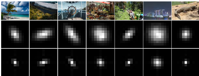
Figure 2. Kernel reformulation examples. The top row and middle row are the LR images and the corresponding primitive kernels. The bottom row is the reformulated kernels.
图 2: 核重构示例。顶行和中行分别是低分辨率 (LR) 图像及其对应的原始核。底行为重构后的核。
• We propose a novel de convolution module named DCLS that is applied on the features as channel-wise deblurring so that we can obtain a clean HR image. • Extensive experiments on various degradation kernels demonstrate that our method leads to state-of-the-art performance in blind SR problems.
• 我们提出了一种名为DCLS的新型反卷积模块,该模块在特征上进行通道级去模糊处理,从而获得清晰的高分辨率(HR)图像。
• 在各种退化核上的大量实验表明,我们的方法在盲超分辨率(SR)问题上实现了最先进的性能。
2. Related work
2. 相关工作
Non-blind SR Since pioneering work SRCNN [6] proposes to learn image SR with a three-layer convolution network, most subsequent works have focused on optimizing the network architectures [5, 10, 17, 18, 21, 28, 32, 40, 43, 55, 59, 61, 62] and loss functions [15, 22, 29, 47, 48, 52, 58]. These CNN-based methods have achieved impressive performance on SISR with a predefined single degradation setting (e.g., bicubic down sampling). However, they may suffer significant performance drops when the predefined degradation kernel is different from the real one.
非盲超分辨率 (Non-blind SR)
自开创性工作 SRCNN [6] 提出用三层卷积网络学习图像超分辨率以来,后续研究大多聚焦于优化网络架构 [5, 10, 17, 18, 21, 28, 32, 40, 43, 55, 59, 61, 62] 和损失函数 [15, 22, 29, 47, 48, 52, 58]。这些基于 CNN 的方法在预设单一退化设置 (如双三次下采样) 的单图像超分辨率 (SISR) 任务中表现出色。然而,当预设退化核与实际退化核不一致时,其性能会显著下降。
Some non-blind SR approaches address the multiple degradation problem by restoring HR images with given the corresponding kernels. Specifically, SRMD [56] is the first method that concatenates LR image with a stretched blur kernel as inputs to obtain a super-resolved image under different degradation s. Later, Zhang et al. [54, 57] incorporate advanced deblurring algorithms and extend the degradation to arbitrary blur kernels. UDVD [51] improves the performance by incorporating dynamic convolution. Hussein et al. [13] introduce a correction filter that transfers blurry LR images to match the bicubicly designed SR model. Besides, zero-shot methods [42, 51] have also been investigated in non-blind SR with multiple degradation s.
一些非盲超分辨率 (SR) 方法通过给定相应核函数来重建高分辨率 (HR) 图像,以解决多重退化问题。具体而言,SRMD [56] 是首个将低分辨率 (LR) 图像与拉伸模糊核拼接作为输入的方法,可在不同退化条件下获得超分辨率图像。随后,Zhang 等人 [54, 57] 结合先进去模糊算法,将退化扩展至任意模糊核。UDVD [51] 通过引入动态卷积提升性能。Hussein 等人 [13] 提出校正滤波器,将模糊 LR 图像转换以匹配双三次设计的 SR 模型。此外,零样本方法 [42, 51] 在多重退化的非盲 SR 领域也得到研究。
Blind SR Under the blind SR setting, HR image is recovered from the LR image degraded with unknown kernel [24, 25, 35]. Most approaches solve this problem with a two stage framework: kernel estimation and kernel-based HR image restoration. For the former, KernelGAN [3] estimates the degradation kernel by utilizing an internal generative adversarial network(GAN) on a single image, and applies that kernel to a non-blind SR approach such as ZSSR to get the SR result. Liang et al. [27] improve the kernel estimating performance by introducing a flow-based prior. Furthermore, Tao et al. [44] propose a spectrum-to-kernel network and demonstrate that estimating blur kernel in the frequency domain is more conducive than in spatial domain. For the latter, Gu et al. [9] propose to apply spatial feature transform (SFT) and iterative kernel correction (IKC) strategy for accurate kernel estimation and SR refinement. Luo et al. [30] develop an end-to-end training deep alternating network (DAN) by estimating reduced kernel and restoring HR image iterative ly. However, both IKC and DAN are time-consuming and computationally costly. The modified version of DAN [31] conducts a dual-path conditional block (DPCB) and supervises the estimator on the complete blur kernel to further improve the performance.
盲超分辨率 (Blind SR)
在盲超分辨率设置下,HR (高分辨率) 图像需从因未知退化核而劣化的LR (低分辨率) 图像中恢复[24, 25, 35]。多数方法通过两阶段框架解决该问题:退化核估计与基于核的HR图像重建。前者中,KernelGAN [3] 利用单幅图像的内部生成对抗网络(GAN)估计退化核,并将该核应用于ZSSR等非盲超分辨率方法以获取结果。Liang等[27] 通过引入基于流的先验提升核估计性能。Tao等[44] 提出频谱到核网络,证明在频域估计模糊核比空间域更具优势。后者中,Gu等[9] 提出采用空间特征变换(SFT)与迭代核校正(IKC)策略实现精确核估计与超分辨率优化。Luo等[30] 通过估计简化核并迭代恢复HR图像,开发了端到端训练的深度交替网络(DAN)。但IKC与DAN均存在耗时与计算成本高的问题。DAN的改进版本[31] 采用双路径条件块(DPCB)并对完整模糊核的估计器进行监督,以进一步提升性能。
3. Method
3. 方法
We now formally introduce our method which consists of three main components given a reformation of degradation: A dynamic deep linear kernel estimation module and a deep constrained least squares module for kernel estimation and LR space feature based deblur. A dual-path network is followed to generate the clean HR output. We will first derive the reformulation and then detail each module.
我们现在正式介绍由三个主要组件组成的退化重构方法:用于核估计和基于LR空间特征去模糊的动态深度线性核估计模块与深度约束最小二乘模块,随后通过双路径网络生成清晰的高分辨率输出。我们将首先推导重构公式,然后详述每个模块。
3.1. Degradation Model Reformulation
3.1. 退化模型重构
Ideally, the blur kernel to be estimated and its corresponding image should be in the same low-resolution space such that the degradation can be transformed to the deblurring problem followed by a SISR problem with bicubic degradation [56, 57]. Towards this end, we propose to reformulate Eq. (1) as
理想情况下,待估计的模糊核及其对应图像应处于同一低分辨率空间,从而将退化问题转化为去模糊问题,再处理为双三次退化的单图像超分辨率(SISR)问题[56, 57]。为此,我们将公式(1)重新表述为
$$
\begin{array}{r l}{\mathbf{y}=\mathcal{F}^{-1}\left(\mathcal{F}\left(\left(\mathbf{x}\mathbf{k}{h}\right){\downarrow_{s}}\right)\right)+\mathbf{n}}\ {\quad=\mathcal{F}^{-1}\left(\mathcal{F}\left(\mathbf{x}{\downarrow_{s}}\right)\frac{\mathcal{F}\left(\left(\mathbf{x}\mathbf{k}{h}\right){\downarrow_{s}}\right)}{\mathcal{F}\left(\mathbf{x}{\downarrow_{s}}\right)}\right)+\mathbf{n}}\ {\quad=\mathbf{x}{\downarrow_{s}}\mathcal{F}^{-1}\left(\frac{\mathcal{F}\left(\left(\mathbf{x}\mathbf{k}{h}\right){\downarrow_{s}}\right)}{\mathcal{F}\left(\mathbf{x}{\downarrow_{s}}\right)}\right)+\mathbf{n},}\end{array}
$$
where $\mathcal{F}$ denotes the Discrete Fourier Transform and ${\mathcal{F}}^{-1}$ denotes its inverse. Then let
其中 $\mathcal{F}$ 表示离散傅里叶变换 (Discrete Fourier Transform),${\mathcal{F}}^{-1}$ 表示其逆变换。然后令
$$
\mathbf{k}{l}=\mathcal{F}^{-1}\left(\frac{\mathcal{F}\left(\left(\mathbf{x}*\mathbf{k}{h}\right){\downarrow s}\right)}{\mathcal{F}\left(\mathbf{x}{\downarrow_{s}}\right)}\right),
$$
we can obtain another form of degradation:
我们可以得到另一种形式的退化:
$$
\mathbf{y}=\mathbf{x}{\downarrow\ast}*\mathbf{k}_{l}+\mathbf{n}.
$$
$$
\mathbf{y}=\mathbf{x}{\downarrow\ast}*\mathbf{k}_{l}+\mathbf{n}.
$$
In the Eq. (6), $\mathbf{k}{l}$ is derived from the corresponding $\mathbf{k}{h}$ and applied on the down sampled HR image ${\bf x}{\downarrow{s}}$ . To ensure numerical stability, we rewrite Eq. (5) with a small regularization parameter $\epsilon$ :
在式 (6) 中,$\mathbf{k}{l}$ 由对应的 $\mathbf{k}{h}$ 推导得出,并应用于下采样的高分辨率图像 ${\bf x}{\downarrow_{s}}$。为确保数值稳定性,我们引入微小正则化参数 $\epsilon$ 重写式 (5):
$$
\mathbf{k}{l}=\mathcal{F}^{-1}\left(\frac{\overline{{\mathcal{F}(\mathbf{x}{\downarrow_{s}})}}}{\overline{{\mathcal{F}(\mathbf{x}{\downarrow_{s}})}}\mathcal{F}(\mathbf{x}{\downarrow_{s}})+\epsilon}\mathcal{F}\left((\mathbf{x}*\mathbf{k}{h}){\downarrow_{s}}\right)\right),
$$
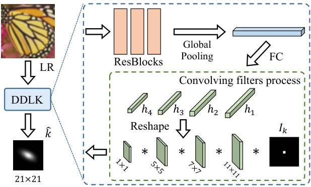
Figure 3. Architecture of the dynamic deep linear kernel.
图 3: 动态深度线性核架构。
where $\overline{{\mathcal{F}(\cdot)}}$ is the complex conjugate of $\mathcal{F}$ . Fig. 2 illustrates the results of reformulating kernels by Eq. (7). Based on the new degradation process, our goal is to estimate the blur kernel $\mathbf{k}_{l}$ and then restore HR image x.
其中 $\overline{{\mathcal{F}(\cdot)}}$ 是 $\mathcal{F}$ 的复共轭。图 2 展示了通过公式 (7) 重构核函数的结果。基于新的退化过程,我们的目标是估计模糊核 $\mathbf{k}_{l}$,然后恢复高分辨率图像 x。
3.2. Dynamic Deep Linear Kernel
3.2. 动态深度线性核
Following the reformation, we start our blind SR method from the kernel estimation. A straightforward solution is to adopt a regression network to estimate kernel $\hat{\mathbf{k}}$ by minimizing the L1 difference w.r.t the new ground-truth blur kernel $\mathbf{k}_{l}$ in Eq. (7). We argue such a single layer kernel (all weights of estimated kernel equal to the ground-truth kernel) estimation is in general difficult and unstable due to the highly non-convex of the blind SR problem [3], leading to kernel mismatch and performance drop [9, 30]. Instead, we propose an image-specific dynamic deep linear kernel (DDLK) which consists of a sequence of linear convolution layers without activation s. Theoretically, deep linear networks have infinitely equivalent global minimas [3, 16, 39], which allow us to find many different filter parameters to achieve the same correct solution. Moreover, since no nonlinearity is used in the network, we can analytically collapse a deep linear kernel as a single layer kernel.
在完成重构后,我们从核估计开始进行盲超分辨率方法。一个直接的解决方案是采用回归网络通过最小化与新真实模糊核$\mathbf{k}_{l}$的L1差异来估计核$\hat{\mathbf{k}}$(如式(7)所示)。我们认为,由于盲超分辨率问题的高度非凸性[3],这种单层核(所有估计核的权重等于真实核)估计通常困难且不稳定,导致核不匹配和性能下降[9, 30]。相反,我们提出了一种图像特定的动态深度线性核(DDLK),它由一系列没有激活函数的线性卷积层组成。理论上,深度线性网络具有无限等效的全局最小值[3, 16, 39],这使我们能够找到许多不同的滤波器参数来实现相同的正确解。此外,由于在网络中没有使用非线性,我们可以解析地将深度线性核折叠为单层核。
Fig. 3 depicts an example of estimating 4 layers dynamic deep linear kernel. The filters are set to $11\times11$ , $7\times7,5\times5$ and $1\times1$ , which make the receptive field to be $21\times21$ . We first generate the filters of each layer based on the LR image, and explicitly sequentially convolve all filters into a single narrow kernel with stride 1. Mathematically, let $\mathbf{h}_{i}$ represent the $i$ -th layer filter, we can get a single layer kernel following
图 3: 展示了一个估算4层动态深度线性核的示例。滤波器尺寸分别设置为 $11\times11$ 、 $7\times7$ 、 $5\times5$ 和 $1\times1$ ,这使得感受野达到 $21\times21$ 。我们首先基于低分辨率(LR)图像生成每层的滤波器,然后以步长1显式地顺序将所有滤波器卷积为单个窄核。用数学表达式表示,设 $\mathbf{h}_{i}$ 代表第 $i$ 层滤波器,可通过以下方式得到单层核:
$$
{\hat{\mathbf{k}}}=\mathbf{I_{k}}\mathbf{h_{1}}\mathbf{h_{2}}\cdot\cdot\cdot\mathbf{h}_{r}
$$
where $r$ is the number of linear layers, $\mathbf{I_{k}}$ is an identity kernel. As an empirically prior, we also constrain the kernel $\hat{\mathbf{k}}$ sum up to 1. The kernel estimation network can be optimized by minimizing the L1 loss between estimated kernel $\hat{\mathbf{k}}$ and new ground-truth blur kernel $\mathbf{k}_{l}$ from Eq. (7).
其中 $r$ 是线性层的数量,$\mathbf{I_{k}}$ 是单位核。根据经验先验,我们还约束核 $\hat{\mathbf{k}}$ 的和为1。通过最小化估计核 $\hat{\mathbf{k}}$ 与来自式(7)的新真实模糊核 $\mathbf{k}_{l}$ 之间的L1损失,可以优化核估计网络。
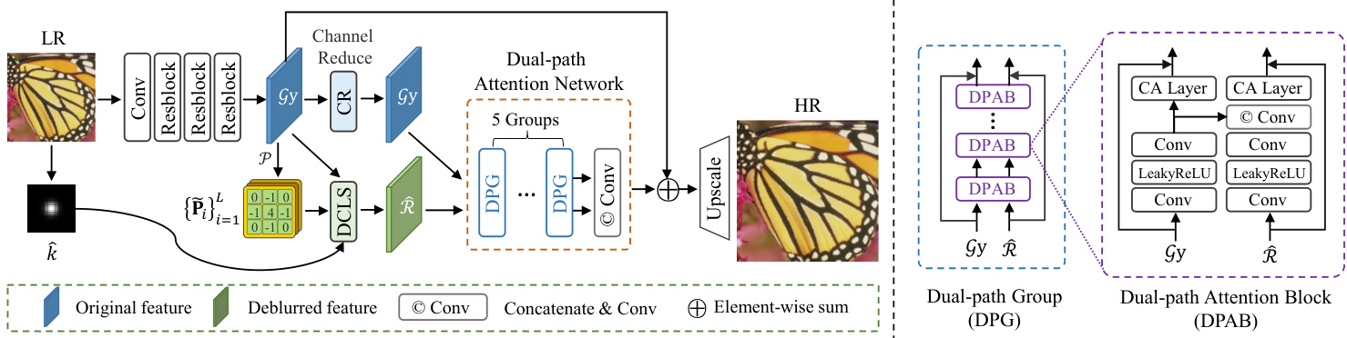
Figure 4. The overview architecture of the proposed method. Given an LR image y, we first estimate the degradation kernel $\hat{\mathbf{k}}$ , and involve it in the deep constrained least squares (DCLS) convolution in the feature domain. The deblurred features $\widehat{\mathcal{R}}$ are then concatenated with primitive features $\mathcal{G}\mathbf{y}$ to restore the clean HR image $\mathbf{x}$ through a dual-path attention network (DPAN).
图 4: 所提方法的整体架构。给定低分辨率(LR)图像y,我们首先估计退化核$\hat{\mathbf{k}}$,并将其应用于特征域中的深度约束最小二乘(DCLS)卷积。去模糊后的特征$\widehat{\mathcal{R}}$随后与原始特征$\mathcal{G}\mathbf{y}$拼接,通过双路径注意力网络(DPAN)恢复出清晰的高分辨率(HR)图像$\mathbf{x}$。
3.3. Deep Constrained Least Squares
3.3. 深度约束最小二乘法
Our goal is to restore HR image based on LR image and estimated kernel $\hat{\mathbf{k}}$ according to the new degradation model (Eq. (6)). Considering a group of feature extracting linear layers ${\mathcal{G}{i}}{i=1}^{L}$ provided to the LR image, we can rewrite Eq. (6) in the feature space, given by
我们的目标是根据新的退化模型(式(6)),基于LR图像和估计核 $\hat{\mathbf{k}}$ 恢复HR图像。考虑到为LR图像提供的一组特征提取线性层 ${\mathcal{G}{i}}{i=1}^{L}$,我们可以在特征空间中重写式(6),得到
$$
\mathcal{G}{i}\mathbf{y}=\hat{\mathbf{k}}\mathcal{G}{i}\mathbf{x}{\downarrow_{s}}+\mathcal{G}_{i}\mathbf{n}.
$$
Let $\widehat{\mathcal{R}}{i}$ be the sought after deblurred feature corresponding to $\mathcal{G}{i}\mathbf{x}{\downarrow_{s}}$ . To solve Eq. (9), we minimize the following criterion function
设 $\widehat{\mathcal{R}}{i}$ 为与 $\mathcal{G}{i}\mathbf{x}{\downarrow_{s}}$ 对应的待求去模糊特征。为求解方程(9),我们最小化以下准则函数
$$
\mathcal{C}=||\nabla\widehat{\mathcal{R}}{i}||^{2},s.t.||\mathcal{G}{i}\mathbf{y}-\widehat{\mathbf{k}}\widehat{\mathcal{R}}{i}||^{2}=||\mathcal{G}_{i}\mathbf{n}||^{2}
$$
where the $\nabla$ is a smooth filter which can be denoted by $\mathbf{P}$ . Then we introduce the Lagrange function, defined by
其中 $\nabla$ 是一个平滑滤波器,可以表示为 $\mathbf{P}$。接着我们引入拉格朗日函数,定义为
$$
\operatorname*{min}{\widehat{\mathcal{R}}{i}}\left[||\mathbf{P}\widehat{\mathcal{R}}{i}||^{2}+\lambda\left(||\mathcal{G}{i}\mathbf{y}-\widehat{\mathbf{k}}\widehat{\mathcal{R}}{i}||^{2}-||\mathcal{G}_{i}\mathbf{n}||^{2}\right)\right],
$$
where $\lambda$ is the Lagrange multiplier. Computing the derivative of Eq. (11) with respect to $\widehat{\mathcal{R}}_{i}$ and setting it to zero:
其中 $\lambda$ 为拉格朗日乘数。对式 (11) 关于 $\widehat{\mathcal{R}}_{i}$ 求导并令其为零:
$$
\left(\lambda\hat{\mathbf{k}}^{\mathsf{T}}\hat{\mathbf{k}}+\mathbf{P}^{\mathsf{T}}\mathbf{P}\right)\boldsymbol{\widehat{\mathcal{R}}}{i}-\lambda\hat{\mathbf{k}}^{\mathsf{T}}\boldsymbol{\mathcal{G}}_{i}\mathbf{y}=0.
$$
We can obtain the clear features as
我们可以获得清晰的特征
$$
{\widehat{\mathcal{R}}}{i}={\mathcal{H}}{\mathcal{G}}_{i}\mathbf{y}.
$$
where $\mathcal{H}_{i}$ denotes the deep constrained least squares deconvolution (DCLS) operator, given by
其中 $\mathcal{H}_{i}$ 表示深度约束最小二乘反卷积 (DCLS) 算子,由
$$
\mathcal{H}=\mathcal{F}^{-1}\left(\frac{\overline{{\mathcal{F}(\hat{\mathbf{k}})}}}{\overline{{\mathcal{F}(\hat{\mathbf{k}})}}\mathcal{F}(\hat{\mathbf{k}})+\frac{1}{\lambda}\overline{{\mathcal{F}(\mathbf{P})}}\mathcal{F}(\mathbf{P})}\right).
$$
$$
\mathcal{H}=\mathcal{F}^{-1}\left(\frac{\overline{{\mathcal{F}(\hat{\mathbf{k}})}}}{\overline{{\mathcal{F}(\hat{\mathbf{k}})}}\mathcal{F}(\hat{\mathbf{k}})+\frac{1}{\lambda}\overline{{\mathcal{F}(\mathbf{P})}}\mathcal{F}(\mathbf{P})}\right).
$$
Different from in the standard image space (e.g. RGB), smooth filter $\mathbf{P}$ and variable $\lambda$ in Eq. (14) might be inconsistent in the feature space. Alternatively, we predict a group
与标准图像空间(如RGB)不同,特征空间中的平滑滤波器$\mathbf{P}$和公式(14)中的变量$\lambda$可能存在不一致性。为此,我们预测了一组
of smooth filters with implicit Lagrange multiplier for different channels through a neural network $\mathcal{P}$ :
通过神经网络 $\mathcal{P}$ 为不同通道实现带有隐式拉格朗日乘子的平滑滤波器
$$
{\tilde{{\bf P}}{i}}{i=1}^{L}={{\mathcal P}(\mathcal{G}{i}{\bf y})}_{i=1}^{L}.
$$
Then the feature-specific operator $\mathcal{H}_{i}$ can be define by
然后特征特定算子 $\mathcal{H}_{i}$ 可以定义为
$$
\mathcal{H}{i}=\mathcal{F}^{-1}\left(\frac{\overline{{\mathcal{F}(\hat{\mathbf{k}})}}}{\overline{{\mathcal{F}(\hat{\mathbf{k}})}}\mathcal{F}(\hat{\mathbf{k}})+\overline{{\mathcal{F}(\tilde{\mathbf{P}}{i})}}\mathcal{F}(\tilde{\mathbf{P}}_{i})}\right).
$$
Now we can obtain the clear features by Eq. (13) and Eq. (16).
现在我们可以通过式(13)和式(16)获得清晰特征。
It is worth to note that a deep neural network (DNN) can be locally linear [7, 23, 36], thus we could apply DNN as $\mathcal{G}_{i}$ to extract useful features in Eq. (9). In addition, the consequent artifacts or errors can be compensated by the following dual-path attention module.
值得注意的是,深度神经网络 (DNN) 在局部可呈现线性特性 [7, 23, 36],因此我们可以将 DNN 作为 $\mathcal{G}_{i}$ 应用于式 (9) 中以提取有效特征。此外,由此产生的伪影或误差可通过后续的双路径注意力模块进行补偿。
3.4. Dual-Path Attention Network
3.4. 双路径注意力网络
Unlike previous works [9, 31] in which the dual-path structures are only used to concatenate the stretched kernel with blurred features, we propose to utilize primitive blur features as additive path to compensate the artifacts and errors introduced by the estimated kernel, known as dual-path attention network (DPAN). DPAN is composed of several groups of dual-path attention blocks (DPAB), it receives both deblurred features $\widehat{\mathcal R}$ and primitive features $\mathcal{G}\mathbf{y}$ . The right of Fig. 4 illustrates tbhe architecture of DPAB.
与先前工作 [9, 31] 仅使用双路径结构将拉伸核与模糊特征拼接不同,我们提出利用原始模糊特征作为附加路径来补偿估计核引入的伪影和误差,称为双路径注意力网络 (DPAN)。DPAN 由多组双路径注意力块 (DPAB) 构成,同时接收去模糊特征 $\widehat{\mathcal R}$ 和原始特征 $\mathcal{G}\mathbf{y}$。图 4 右侧展示了 DPAB 的结构。
Since the additive path of processing $\mathcal{G}\mathbf{y}$ is independently updated and used to concatenate with R to provide primary information to refine the dec on vol ved fbeatures. We can reduce its channels to accelerate training and inference, as the channel reduction (CR) operation illustrated in left of Fig. 4. Moreover, on the dec on vol ved feature path, we apply the channel attention layer [60] after aggregating original features. In addition, we add a residual connection for each path on all groups and blocks. The pixel shuffle [11] is used as the upscale module. We can jointly optimize the SR network and kernel estimation network as follows:
由于处理 $\mathcal{G}\mathbf{y}$ 的加法路径是独立更新并与 R 拼接以提供主要信息来优化解卷积特征,我们可以通过通道缩减 (channel reduction, CR) 操作(如图 4 左侧所示)减少其通道数以加速训练和推理。此外,在解卷积特征路径上,我们在聚合原始特征后应用通道注意力层 [60]。同时,我们在所有组和块中的每条路径上添加了残差连接,并使用像素洗牌 (pixel shuffle) [11] 作为上采样模块。超分辨率网络与核估计网络的联合优化可表示为:
Table 1. Quantitative comparison on datasets with Gaussian8 kernels. The best two results are marked in red and blue colors, respective
表 1: 采用高斯核(Gaussian8)数据集的定量比较。最优的两个结果分别用红色和蓝色标出
| 方法 | 尺度 | Set5 [4] | Set14 [53] | BSD100 [33] | Urban100 [12] | Manga109 [34] |
|---|---|---|---|---|---|---|
| PSNR | SSIM | PSNR | SSIM | PSNR | ||
| Bicubic | 28.82 | 0.8577 | 26.02 | 0.7634 | 25.92 | |
| CARN [2] | x2 | 30.99 | 0.8779 | 28.10 | 0.7879 | 26.78 |
| Bicubic+ZSSR [41] | x2 | 31.08 | 0.8786 | 28.35 | 0.7933 | 27.92 |
| Deblurring [37]+CARN [41] | x2 | 24.20 | 0.7496 | 21.12 | 0.6170 | 22.69 |
| CARN [41]+Deblurring [37] | x2 | 31.27 | 0.8974 | 29.03 | 0.8267 | 28.72 |
| IKC [9] | x2 | 37.19 | 0.9526 | 32.94 | 0.9024 | 31.51 |
| DANv1 [30] | x2 | 37.34 | 0.9526 | 33.08 | 0.9041 | 31.76 |
| DANv2 [31] | x2 | 37.60 | 0.9544 | 33.44 | 0.9094 | 32.00 |
| DCLS(本文) | x2 | 37.63 | 0.9554 | 33.46 | 0.9103 | 32.04 |
| Bicubic | x3 | 26.21 | 0.7766 | 24.01 | 0.6662 | 24.25 |
| CARN [2] | x3 | 27.26 | 0.7855 | 25.06 | 0.6676 | 25.85 |
| Bicubic+ZSSR [41] | x3 | 28.25 | 0.5226 | 26.15 | 0.6942 | 26.06 |
| Deblurring [37]+CARN [41] | x3 | 19.05 | 17.61 | 0.4558 | 20.51 | |
| CARN [41]+Deblurring [37] | x3 | 30.31 | 0.8562 | 27.57 | 0.7531 | 27.14 |
| IKC [9] | x3 | 33.06 | 0.9146 | 29.38 | 0.8233 | 28.53 |
| DANv1 [30] | x3 | 34.04 | 0.9199 | 30.09 | 0.8287 | 28.94 |
| DANv2 [31] | x3 | 34.12 | 0.9209 | 30.20 | 0.8309 | 29.03 |
| DCLS(本文) | x3 | 34.21 | 0.9218 | 30.29 | 0.8329 | 29.07 |
| Bicubic | x4 | 24.57 | 0.7108 | 22.79 | 0.6032 | 23.29 |
| CARN [2] | x4 | 26.57 | 0.7420 | 24.62 | 0.6226 | 24.79 |
| Bicubic+ZSSR [41] | x4 | 26.45 | 0.7279 | 24.78 | 0.6268 | 24.97 |
| Deblurring [37]+CARN [41] | x4 | 18.10 | 0.4843 | 16.59 | 0.3994 | 18.46 |
| CARN [41]+Deblurring [37] | x4 | 28.69 | 0.8092 | 26.40 | 0.6926 | 26.10 |
| IKC [9] | x4 | 31.67 | 0.8829 | 28.31 | 0.7643 | 27.37 |
| DANv1 [30] | x4 | 31.89 | 0.8864 | 28.42 | 0.7687 | 27.51 |
| DANv2 [31] | x4 | 32.00 | 0.8885 | 28.50 | 0.7715 | 27.56 |
| AdaTarget [14] | x4 | 31.58 | 0.8814 | 28.14 | 0.7626 | 27.43 |
| DCLS(本文) | x4 | 32.12 | 0.8890 | 28.54 | 0.7728 | 27.60 |
Table 2. Quantitative comparison on various noisy datasets. The best one marks in red and the second best are in blue.
| 方法 x4 | 噪声水平 | Set5 [4] PSNR | Set5 [4] SSIM | Set14 [53] PSNR | Set14 [53] SSIM | BSD100 [33] PSNR | BSD100 [33] SSIM | Urban100 [12] PSNR | Urban100 [12] SSIM | Manga109[34] PSNR | Manga109[34] SSIM |
|---|---|---|---|---|---|---|---|---|---|---|---|
| Bicubic+ZSSR[41] | 15 | 23.32 | 0.4868 | 22.49 | 0.4256 | 22.61 | 0.3949 | 20.68 | 0.3966 | 22.04 | 0.4952 |
| IKC [9] | 15 | 26.89 | 0.7671 | 25.28 | 0.6483 | 24.93 | 0.6019 | 22.94 | 0.6362 | 25.09 | 0.7819 |
| DANv1 [30] | 15 | 26.95 | 0.7711 | 25.27 | 0.6490 | 24.95 | 0.6033 | 23.00 | 0.6407 | 25.29 | 0.7879 |
| DANv2 [31] | 15 | 26.97 | 0.7726 | 25.29 | 0.6497 | 24.95 | 0.6025 | 23.03 | 0.6429 | 25.32 | 0.7896 |
| DCLS(本文) | 15 | 27.14 | 0.7775 | 25.37 | 0.6516 | 24.99 | 0.6043 | 27.13 | 0.6500 | 25.57 | 0.7969 |
| Bicubic+ZSSR[41] | 19.77 | 0.2938 | 19.36 | 0.2534 | 19.43 | 0.2308 | 18.32 | 0.2450 | 19.25 | 0.3046 | |
| IKC [9] | 25.27 | 0.7154 | 24.15 | 0.6100 | 24.06 | 0.5674 | 22.11 | 0.5969 | 23.80 | 0.7438 | |
| DANv1 [30] | 25.32 | 0.7276 | 24.15 | 0.6138 | 24.04 | 0.5678 | 22.08 | 0.5977 | 23.82 | 0.7442 | |
| DANv2 [31] | 25.36 | 0.7264 | 24.16 | 0.6121 | 24.06 | 0.5690 | 22.14 | 0.6014 | 23.87 | 0.7489 | |
| DCLS(本文) | 25.49 | 0.7323 | 24.23 | 0.6131 | 24.09 | 0.5696 | 22.37 | 0.6119 | 24.21 | 0.7582 |
表 2. 不同噪声数据集上的定量比较。最优结果标红,次优结果标蓝。
$$
\mathcal{L}=l_{1}(\hat{\mathbf{k}},\mathbf{k}{l};\theta{k})+l_{1}(\hat{\mathbf{x}},\mathbf{x};\theta_{g})
$$
$$
\mathcal{L}=l_{1}(\hat{\mathbf{k}},\mathbf{k}{l};\theta{k})+l_{1}(\hat{\mathbf{x}},\mathbf{x};\theta_{g})
$$
where $\theta_{k}$ and $\theta_{g}$ are the parameters of kernel estimation net- work and DCLS reconstruction network, respectively.
其中 $\theta_{k}$ 和 $\theta_{g}$ 分别是核估计网络和 DCLS 重建网络的参数。
4. Experiments
4. 实验
4.1. Datasets and Implementation Details
4.1. 数据集与实现细节
Following previous works [9, 30], 3450 2K HR images from DIV2K [1] and Flickr2K [45] are collected as the training dataset. And we synthesize corresponding LR images with specific degradation kernel settings (e.g., isotropic/anisotropic Gaussian) using Eq. (1). The proposed method is evaluated by PSNR and SSIM [49] on only the luminance channel of the SR results (YCbCr space).
遵循先前工作[9, 30],我们从DIV2K[1]和Flickr2K[45]中收集了3450张2K高清(HR)图像作为训练数据集,并使用公式(1)通过特定退化核设置(如各向同性/异性高斯核)合成对应的低分辨率(LR)图像。所提方法仅在超分辨率结果的亮度通道(YCbCr空间)上通过PSNR和SSIM[49]进行评估。
Isotropic Gaussian kernels. Firstly, we conduct blind SR experiments on isotropic Gaussian kernels following the setting in [9]. Specifically, the kernel sizes are fixed to $21\times21$ . In training, we uniformly sample the kernel width from range [0.2, 2.0], [0.2, 3.0] and [0.2, 4.0] for SR scale factors 2, 3 and 4, respectively. For testing, we use
各向同性高斯核 (isotropic Gaussian kernels)。首先,我们按照[9]中的设置对各向同性高斯核进行盲超分实验。具体而言,核大小固定为$21\times21$。训练时,对于2倍、3倍和4倍超分比例,我们分别从[0.2, 2.0]、[0.2, 3.0]和[0.2, 4.0]范围内均匀采样核宽度。测试时,我们使用

Figure 5. The PSNR performance curves on Set5 and Manga109 of scale factor 4. The kernel width $\sigma$ are set from 1.8 to 3.2.
图 5: 在Set5和Manga109数据集上4倍放大因子的PSNR性能曲线。核宽度$\sigma$取值从1.8到3.2。

Figure 6. Visual results of Img 33 from Urban100.
图 6: Urban100数据集中Img 33的可视化结果
Gaussian8 [9] kernel setting to generate evaluation dataset from five widely used benchmarks: Set5 [4], Set14 [53], BSD100 [33], Urban100 [12] and Manga109 [34]. Gaussian8 uniformly chooses 8 kernels from range [0.80, 1.60], [1.35, 2.40] and [1.80, 3.20] for scale factors 2, 3 and 4, rep ect iv ely. The LR images are obtained by blurring and down sampling the HR images with selected kernels.
Gaussian8 [9] 核设置从五个广泛使用的基准测试集生成评估数据集:Set5 [4]、Set14 [53]、BSD100 [33]、Urban100 [12] 和 Manga109 [34]。对于缩放因子2、3和4,Gaussian8分别从范围[0.80, 1.60]、[1.35, 2.40]和[1.80, 3.20]中均匀选择8个核。低分辨率(LR)图像是通过使用选定的核模糊并下采样高分辨率(HR)图像获得的。
Anisotropic Gaussian kernels. We also conduct experiments on anisotropic Gaussian kernels following the setting in [3]. The kernel size is set to $11~\times 11$ and $31~\times$ 31 for scale factors 2 and 4, respectively. During training, the anisotropic Gaussian kernels for degradation are generated by randomly selecting kernel width from range (0.6, 5) and rotating from range $[-\pi,\pi]$ . We also apply uniform multiplicative noise and normalize it to sum to one. For evaluation, we use the DIV2KRK dataset proposed in [3].
各向异性高斯核。我们按照[3]中的设置对各向异性高斯核进行了实验。对于缩放因子2和4,核大小分别设置为$11~\times 11$和$31~\times~31$。训练过程中,通过从范围(0.6, 5)随机选择核宽度、从范围$[-\pi,\pi]$随机旋转来生成退化的各向异性高斯核。我们还应用了均匀乘性噪声并将其归一化为总和为一。评估时,我们使用了[3]提出的DIV2KRK数据集。
Implementation details. For all experiments, we use 5 dual-path groups, each containing 10 DPABs with 64 channels. The batch sizes are set to 64 and the LR patch sizes are $64\times64$ . We use Adam [20] optimizer with $\beta_{1}=0.9$ and $\beta_{2}=0.99$ . All models are trained on 4 RTX2080Ti GPUs with $5\times10^{5}$ iterations. The initial learning rate is set to $4\times10^{-4}$ and decayed by half at every $2\times10^{-4}$ iterations. We also augment the training data with random horizontal flips and 90 degree rotations.
实现细节。所有实验中,我们使用5个双路径组,每组包含10个64通道的DPAB。批处理大小设置为64,低分辨率 (LR) 图像块尺寸为 $64\times64$ 。采用Adam [20] 优化器,参数设为 $\beta_{1}=0.9$ 和 $\beta_{2}=0.99$ 。所有模型均在4块RTX2080Ti GPU上训练 $5\times10^{5}$ 次迭代,初始学习率为 $4\times10^{-4}$ ,每 $2\times10^{4}$ 次迭代衰减一半。训练数据通过随机水平翻转和90度旋转进行增强。
4.2. Comparison with State-of-the-arts
4.2. 与现有最优方法的对比
Evaluation with isotropic Gaussian kernels. Following [9], we evaluate our method on datasets synthesized by Gaussian8 kernels. We compare our method with stateof-the-art blind SR approaches: ZSSR [41] (with bicubic kernel), IKC [9], DANv1 [30], DANv2 [31] and AdaTarget [14]. Following [9], we also conduct comparison with CARN [2] and its variants of performing blind deblurring method [37] before and after CARN. For most methods, we use their official implementations and pre-trained models.
采用各向同性高斯核进行评估。参照[9],我们在由Gaussian8核合成的数据集上评估了我们的方法。我们将本方法与以下最先进的盲超分辨率(SR)方法进行了比较:ZSSR[41](使用双三次核)、IKC[9]、DANv1[30]、DANv2[31]和AdaTarget[14]。根据[9]的设定,我们还与CARN[2]及其变体(在CARN前后执行盲去模糊方法[37])进行了对比。对于多数方法,我们采用了其官方实现和预训练模型。
Table 3. Quantitative comparison on DIV2KRK. The best one marks in red and the second best are in blue.
| 方法 | DIV2KRK [3] (x2) | DIV2KRK [3] (X4) | ||
|---|---|---|---|---|
| PSNR | SSIM | PSNR | SSIM | |
| Bicubic | 28.73 | 0.8040 | 25.33 | 0.6795 |
| Bicubic+ZSSR[41] | 29.10 | 0.8215 | 25.61 | 0.6911 |
| EDSR [28] | 29.17 | 0.8216 | 25.64 | 0.6928 |
| RCAN [59] | 29.20 | 0.8223 | 25.66 | 0.6936 |
| DBPN [10] | 29.13 30.38 | 0.8190 | 25.58 | 0.6910 |
| DBPN[10]+Correction [13] | 29.57 | 0.8717 0.8564 | 26.79 27.51 | 0.7426 0.7265 |
| KernelGAN [3]+SRMD [56] KernelGAN[3]+ZSSR[41] | 30.36 | 0.8669 | 26.81 | 0.7316 |
| IKC [9] | 27.70 | 0.7668 | ||
| DANv1 [30] | 32.56 | 0.8997 | 27.55 | 0.7582 |
| DANv2 [31] | 32.58 | 0.9048 | 28.74 | 0.7893 |
| AdaTarget [14] | 28.42 | 0.7854 | ||
| KOALAnet[19] | 31.89 | 0.8852 | 27.77 | 0.7637 |
| DCLS(Ours) | 32.75 | 0.9094 | 28.99 | 0.7946 |
表 3. DIV2KRK数据集上的量化对比。最优结果标红,次优结果标蓝。

Figure 7. Visual results of estimated kernels of Img 33 and Img 43 from DIV2KRK [3] by various kernel estimation methods.
Table 4. Quantitative evaluation on the performance of DDLK.
图 7: 不同核估计方法对DIV2KRK [3]中Img 33和Img 43的估计核可视化结果。
| DIV2KRK x4 | KernelGAN | CorrFilter | DANv2 | DDLK |
|---|---|---|---|---|
| LR-PSNR↑ | 41.28 | 41.35 | 45.06 | 45.27 |
| Kernel-MSE ← | 0.1518 | 0.1392 | 0.0817 | 0.0574 |
表 4: DDLK性能的定量评估。
The quantitative results are shown in Table 1. It is obvious that our method leads to the best performance over all datasets. The bicubic SR model CARN suffers severe performance drop with Gaussian8 which deviates from the predefined bicubic kernel. Performing deblurring on the superresolved image can improve the results. ZSSR achieves better performance compared with non-blind SR method but is limited by the image-specific network design (cannot utilize abundant training data). AdaTarget can improve image quality but is still inferior to that of blind SR methods. IKC and DAN are two-step blind SR methods and can largely improve the results. However, both of them predict kernel embedding and directly involve it into the network, which damages the spatial relation of the kernel and thus performs inferior to our method. We also provide the comparison of PSNR values on different datasets with blur kernels width from 1.8 to 3.2 as shown in Fig. 5. DCLS performs the best result over all different kernel widths. The qualitative results shown in Fig. 8 illustrate that DCLS can produce clear and pleasant SR images. Furthermore, we conduct an experiment of super-resolving images with additional noise. As shown in Table 2 and Fig. 6, DCLS still outperforms other methods over all datasets with different noise levels.
定量结果如表1所示。显然,我们的方法在所有数据集上都取得了最佳性能。基于双三次插值的超分辨率模型CARN在偏离预设双三次核的Gaussian8上表现严重下滑。对超分辨率图像进行去模糊处理可以改善结果。ZSSR相比非盲超分辨率方法表现更优,但受限于图像特定网络设计(无法利用丰富训练数据)。AdaTarget能提升图像质量,但仍逊色于盲超分辨率方法。IKC和DAN作为两步式盲超分辨率方法能显著改善结果,但两者都通过预测核嵌入并直接引入网络,破坏了核的空间关系,因此表现不及我们的方法。图5展示了不同数据集在1.8至3.2模糊核宽度下的PSNR值对比,DCLS在所有核宽度下均取得最优结果。图8的定性结果表明DCLS能生成清晰悦目的超分辨率图像。此外,我们对含附加噪声的图像进行超分辨率实验,如表2和图6所示,DCLS在不同噪声水平的所有数据集上仍优于其他方法。

Figure 8. Visual results of Img 67 and Img 73 in Urban100 [12], for scale factor 4 and kernel width 2.6. Best viewed in color.
图 8: Urban100 [12] 中 Img 67 和 Img 73 在缩放因子 4 和核宽度 2.6 下的视觉效果对比。建议彩色查看。

Figure 9. Visual results of Img 36 and Img 12 in DIV2KRK [3], for scale factor of 4. Best viewed in color.
图 9: DIV2KRK [3] 中 Img 36 和 Img 12 在 4 倍缩放因子下的可视化结果。建议彩色查看。
Evaluation with anisotropic Gaussian kernels. Degradation with anisotropic Gaussian kernels are more general and challenging. Similar to isotropic kernel, we firstly compare our method with SOTA blind SR approaches such as ZSSR [41], IKC [9], DANv1 [30], DANv2 [31], AdaTarget [14] and KOALAnet [19]. We also compare DCLS with some SOTA bicubicly designed methods such as EDSR [28], RCAN [59], and DBPN [10]. And we pro- vide Correction [13] for DBPN. In addition, we combine a kernel estimation method (e.g. KernelGAN [3]) with other non-blind SR methods, such as ZSSR [41] and SRMD [56], as two-step solutions to solve blind SR.
使用各向异性高斯核进行评估。各向异性高斯核的退化更为普遍且具有挑战性。与各向同性核类似,我们首先将我们的方法与ZSSR [41]、IKC [9]、DANv1 [30]、DANv2 [31]、AdaTarget [14] 和KOALAnet [19] 等最先进的盲超分辨率方法进行比较。我们还比较了DCLS与一些最先进的双三次设计方法,如EDSR [28]、RCAN [59] 和DBPN [10],并为DBPN提供了修正 [13]。此外,我们将核估计方法(如KernelGAN [3])与其他非盲超分辨率方法(如ZSSR [41] 和SRMD [56])结合,作为解决盲超分辨率的两步解决方案。
Table 3 shows the quantitative results on DIV2KRK [3]. It can be seen that the proposed DCLS significantly improves the performance compared with other blind SR approaches. Note that ZSSR performs better when combined with KernelGAN, which indicates that good kernel estimation can help a lot. Recent SOTA blind SR methods such as IKC, DAN and KOALAnet can achieve remarkable accuracy in PSNR and SSIM. By applying an adaptive target to finetune the network, AdaTarget can perform comparably with SOTA blind methods. However, all of those methods are still inferior to the proposed DCLS. The visual results on DIV2KRK are shown in Fig. 9. As we can see, the SR images produced by our method are much sharper and cleaner. We also provide the results of kernel estimation and down sampling HR image with estimated kernel in Fig. 7 and Table 4. Compared with previous image-specific methods such as KernelGAN [3] and Correction Filter [13], the dynamic deep linear kernel (DDLK) is more flexible and capable of producing accurate kernels.
表 3 展示了 DIV2KRK [3] 的量化结果。可以看出,相比其他盲超分辨率方法,提出的 DCLS 显著提升了性能。值得注意的是,当 ZSSR 与 KernelGAN 结合时表现更好,这表明良好的核估计能带来很大帮助。最近的 SOTA 盲超分辨率方法如 IKC、DAN 和 KOALAnet 在 PSNR 和 SSIM 指标上取得了显著精度。通过采用自适应目标对网络进行微调,AdaTarget 的表现与 SOTA 盲方法相当。然而,这些方法仍逊色于提出的 DCLS。DIV2KRK 的视觉结果如图 9 所示。可以看出,本方法生成的超分辨率图像更清晰、更干净。我们还在图 7 和表 4 中提供了核估计结果以及使用估计核下采样高分辨率图像的结果。与 KernelGAN [3] 和 Correction Filter [13] 等先前的图像专用方法相比,动态深度线性核 (DDLK) 更灵活且能生成更准确的核。
Table 5. Ablation study on our vital components.
表 5: 核心组件消融实验
| SLK | DDLK | Stretching Strategy | DCLS Deconv | DPAN | DIV2KRK PSNR | DIV2KRK SSIM |
|---|---|---|---|---|---|---|
| √ | 28.84 | 0.7921 | ||||
| √ | √ | 28.86 | 0.7924 | |||
| √ | 28.94 | 0.7946 | ||||
| √ | 28.94 | 0.7938 | ||||
| √ | √ | √ | 28.99 | 0.7964 |
Table 6. Quantitative comparison on various datasets. Fea means applying de convolution on the feature space.
表 6: 不同数据集上的定量比较。Fea表示在特征空间应用反卷积。
| 方法 | WienerFea [7] PSNR | WienerFea [7] SSIM | CLSFea PSNR | CLSFea SSIM | DCLSFea PSNR | DCLSFea SSIM |
|---|---|---|---|---|---|---|
| Set5 | 32.05 | 0.8878 | 31.98 | 0.8862 | 32.12 | 0.8890 |
| Set14 | 28.38 | 0.7709 | 28.29 | 0.7658 | 28.54 | 0.7728 |
| BSD100 | 27.47 | 0.7238 | 27.48 | 0.7216 | 27.60 | 0.7285 |
| Urban100 | 26.07 | 0.7775 | 26.03 | 0.7768 | 26.15 | 0.7809 |
| Manga109 | 30.77 | 0.9069 | 30.65 | 0.9040 | 30.86 | 0.9086 |
| DIV2KRK | 28.77 | 0.7886 | 28.92 | 0.7921 | 28.99 | 0.7947 |
Table 7. Quantitative results. RGB and Fea mean applying deconvolution in the RGB space and feature space, respectively.
表 7: 定量结果。RGB和Fea分别表示在RGB空间和特征空间应用反卷积。
| DIV2KRK x4 | WienerRGB | CLSRGB | DCLSRGB | DCLSFea |
|---|---|---|---|---|
| PSNR | 28.91 | 28.90 | 28.94 | 28.99 |
| SSIM | 0.7941 | 0.7935 | 0.7941 | 0.7964 |
4.3. Analysis and Discussions
4.3. 分析与讨论
Ablation Study. We conduct ablation studies on vital components of our method: DPAN, DDLK and DCLS deconvolution. The quantitative results on DIV2KRK are exported in Table 5. Note that the baseline model with DPAN eliminates artifacts from kernel and thus improves the result. And the DCLS de convolution can further make use of the estimated kernel and high-level information from deep features to achieve a higher performance $(+0.15\mathrm{dB}$ from baseline).
消融实验。我们对方法的核心组件进行了消融研究:DPAN、DDLK和DCLS反卷积。DIV2KRK上的量化结果如表5所示。需要注意的是,带有DPAN的基线模型消除了核(kernel)带来的伪影,从而提升了结果。而DCLS反卷积能进一步利用估计核和深层特征中的高层级信息实现更高性能(较基线提升+0.15dB)。
Effectiveness of the DCLS de convolution. To illustrate the effectiveness of DCLS, we include a comparison of substituting DCLS with other deblurring methods, such as traditional constrained least squares (CLS) and Wiener deconvolution [7, 50] in the RGB space and feature space. The results are presented in Table 6 and Table 7. By applying de convolution in the RGB space with the reformulated kernel, we can get a clear LR image and thus improve the SR performance. This idea is similar to Correction Filter [13], but with one big difference, in that our estimator is highly correlated to the LR image rather than the SR model. The visual example is shown in Fig. 10.
DCLS去卷积的有效性。为说明DCLS的有效性,我们比较了在RGB空间和特征空间中使用其他去模糊方法(如传统约束最小二乘法(CLS)和维纳去卷积[7,50])替代DCLS的效果,结果如表6和表7所示。通过使用重构核在RGB空间进行去卷积,我们可以获得清晰的低分辨率(LR)图像,从而提升超分辨率(SR)性能。该思路与校正滤波器[13]类似,但存在一个关键差异:我们的估计器与LR图像高度相关,而非SR模型。可视化示例如图10所示。

Figure 10. Applying DCLS in the RGB space. (a) Original LR & kernel, (b) corrected LR & estimated kernel by [13], (c) deblurred LR & estimated kernel by the proposed method.
图 10: 在RGB空间应用DCLS的效果。(a) 原始低分辨率图像及模糊核,(b) 通过[13]方法校正后的低分辨率图像及估计模糊核,(c) 本文方法去模糊后的低分辨率图像及估计模糊核。

Figure 11. Comparison of historic image [21] for $4\times$ SR.
图 11: 历史图像[21]在4倍超分辨率(SR)下的对比
Performance on Real Degradation To further demonstrate the effectiveness of our method, we apply the proposed model on real degradation data where the ground truth HR images and the blur kernels are not available. An example of super-resolving historic image is shown in Fig. 11. Compared with LapSRN [21] and DANv2 [31], our DCLS can produce sharper edges and visual pleasing SR results.
真实退化场景下的性能表现
为进一步验证本方法的有效性,我们将所提模型应用于真实退化数据(其中高清真值图像和模糊核均不可得)。图11展示了历史图像超分辨率重建的实例。与LapSRN [21]和DANv2 [31]相比,我们的DCLS能生成更锐利的边缘和视觉观感更佳的超分结果。
5. Conclusion
5. 结论
In this work, we have presented a well-principled algorithm to tackle the blind SR problem. We first derive a new form of blur kernel in the low resolution space from classical degradation model. We then propose to estimate and apply that kernel in HR image restoration. Subsequently, a dynamic deep linear kernel (DDLK) module is introduced to improve kernel estimation. We further design a deep constrained least squares (DCLS) de convolution module that integrates blur kernel and LR image in the feature domain to obtain the clean feature. The clean feature and the primitive feature are then fed into a dual-path network to generate the super-resolved image. Extensive experiments on various kernels and noises demonstrate that the proposed method leads to a state-of-the-art blind SR performance.
在这项工作中,我们提出了一种原理完善的算法来解决盲超分辨率(SR)问题。首先从经典退化模型中推导出低分辨率空间下模糊核的新形式,随后提出在高分辨率图像恢复中估计并应用该核。接着引入动态深度线性核(DDLK)模块来优化核估计。我们进一步设计了深度约束最小二乘(DCLS)反卷积模块,将模糊核与低分辨率图像在特征域中融合以获取清洁特征。清洁特征与原始特征随后被输入双路径网络,最终生成超分辨率图像。针对多种核函数与噪声的大量实验表明,该方法实现了当前最先进的盲超分辨率性能。