THE CHRONICLES OF RAG: THE RETRIEVER, THE CHUNK AND THE GENERATOR
RAG编年史:检索器、文本块与生成器
PREPRINT
预印本
∗Paulo Finardi
*Paulo Finardi
∗Leonardo Avila Marcos Piau
Leonardo Avila Marcos Piau
Rodrigo Castaldoni Pablo Costa
Rodrigo Castaldoni Pablo Costa
Pedro Gengo Vinicius Caridá
Pedro Gengo Vinicius Caridá
22h, Brazil
22小时,巴西
email: {pfinardi, leonardo.bernardi.avila, cast aldo niro, pedro.gengo.lourenco, cel i ol archer, marcos.piau.vieira, pablo.botton.costa, vfcarida}@gmail.com
email: {pfinardi, leonardo.bernardi.avila, castaldo.niro, pedro.gengo.lourenco, celio.archer, marcos.piau.vieira, pablo.botton.costa, vfcarida}@gmail.com
∗ Both authors contributed equally to this research.
∗ 两位作者对本研究的贡献均等。
ABSTRACT
摘要
Retrieval Augmented Generation (RAG) has become one of the most popular paradigms for enabling LLMs to access external data, and also as a mechanism for grounding to mitigate against hallucinations. When implementing RAG you can face several challenges like effective integration of retrieval models, efficient representation learning, data diversity, computational efficiency optimization, evaluation, and quality of text generation. Given all these challenges, every day a new technique to improve RAG appears, making it unfeasible to experiment with all combinations for your problem. In this context, this paper presents good practices to implement, optimize, and evaluate RAG for the Brazilian Portuguese language, focusing on the establishment of a simple pipeline for inference and experiments. We explored a diverse set of methods to answer questions about the first Harry Potter book. To generate the answers we used the OpenAI’s gpt-4, gpt-4-1106-preview, gpt-3.5-turbo-1106, and Google’s Gemini Pro. Focusing on the quality of the retriever, our approach achieved an improvement of $\mathbf{MRR}@10$ by $35.4%$ compared to the baseline. When optimizing the input size in the application, we observed that it is possible to further enhance it by $2.\dot{4}%$ . Finally, we present the complete architecture of the RAG with our recommendations. As result, we moved from a baseline of $5\bar{7}.88%$ to a maximum relative score of $98.61%$ .
检索增强生成 (Retrieval Augmented Generation, RAG) 已成为大语言模型访问外部数据的主流范式之一,同时也作为缓解幻觉的落地机制。在实现RAG时,开发者可能面临多重挑战:检索模型的有效集成、高效的表示学习、数据多样性、计算效率优化、评估体系以及文本生成质量。鉴于这些挑战,每天都有新的RAG改进技术涌现,使得针对具体问题穷尽所有组合实验变得不切实际。
本文针对巴西葡萄牙语场景,提出了实现、优化和评估RAG的最佳实践,重点构建了一个简洁的推理与实验流程。我们采用多样化方法解答关于《哈利·波特》首部曲的问题,答案生成环节使用了OpenAI的gpt-4、gpt-4-1106-preview、gpt-3.5-turbo-1106以及Google的Gemini Pro模型。通过优化检索器质量,我们的方法在$\mathbf{MRR}@10$指标上较基线提升$35.4%$。在应用层面对输入规模进行优化时,我们发现仍有$2.\dot{4}%$的提升空间。最终呈现的完整RAG架构包含我们的改进建议,使得相对评分从基线$5\bar{7}.88%$提升至最高$98.61%$。
1 Introduction
1 引言
The rise of Large Language Models (LLMs) has changed the way we approach Artificial Intelligence (AI) applications. Their ability to answer different user queries in different domains allow these models to show a notable performance in a wide range of tasks like translation, summarizing, question answering, and many others [1]. However, there are a lot of open challenges when it comes to problems that require answers based on updated information, and external data, that were not available in the training data.
大语言模型 (LLM) 的崛起改变了我们开发人工智能 (AI) 应用的方式。这些模型能够回答不同领域的用户查询,使其在翻译、摘要、问答等广泛任务中展现出卓越性能 [1]。然而,当涉及需要基于训练数据中未包含的更新信息和外部数据来解答的问题时,仍存在诸多开放挑战。
In order to overcome this challenge, a technique called Retrieval Augmented Generation (RAG) [2] was developed. This approach aims to solve the limitation of the need for external data, by fetching and incorporating this information in the prompt. With this, the model can generate more cohesive answers about subjects and data not seen during the training, decreasing the occurrence of hallucinations [3]. Nevertheless, this approach adds a new layer of challenges since it requires the development of a trustworthy retriever pipeline, given that the quality of the final answer can be highly affected if the retrieved text is not relevant to the user query [4].
为了克服这一挑战,人们开发了一种称为检索增强生成 (Retrieval Augmented Generation, RAG) [2] 的技术。该方法通过获取外部数据并将其融入提示词,旨在解决模型依赖外部数据的局限性。这使得模型能够针对训练阶段未接触的主题和数据生成更具连贯性的回答,从而减少幻觉 (hallucination) [3] 的发生。然而,该方法也引入了新的挑战——由于最终回答质量会因检索文本与用户查询的相关性而显著波动 [4],因此需要构建可靠的检索器 (retriever) 管道。
The landscape of RAG is rapidly expanding, with a constant influx of new papers introducing diverse implementations [5]. Each of these variants proposes technical modifications or enhancements, such as different retrieval mechanisms, augmentation techniques, or fine-tuning methodologies. This proliferation, while a testament to the field’s dynamism, presents a substantial challenge for AI practitioners. The task of methodically experimenting with, and critically evaluating, each variant’s performance, s cal ability, and applicability becomes increasingly complex.
RAG (Retrieval-Augmented Generation) 领域正在快速扩张,不断有新论文提出多样化的实现方案 [5]。这些变体各自提出了技术改进或增强,例如不同的检索机制、增强技术或微调方法。这种激增现象虽然证明了该领域的活力,但也给AI从业者带来了重大挑战。系统性地实验并批判性评估每个变体的性能、可扩展性和适用性,这一任务正变得日益复杂。
In this paper, we present a comprehensive series of experiments focused on the application of RAG specifically tailored for Brazilian Portuguese. Our research delves into evaluating various retrieval techniques, including both sparse and dense retrievers. Additionally, we explore two chunking strategies (naive and sentence window) to optimize the integration of retrieved information into the generation process. We also investigate the impact of the positioning of documents within the prompt, analyzing how this influences the overall quality and relevance of the generated content. Finally, our experiments extend to comparing the performance of different LLMs, notably GPT-4 and Gemini, in their ability to effectively incorporate the retrieved information and produce coherent, con textually accurate responses. This paper aims to provide valuable insights and practical guidelines for implementing RAG in Brazilian Portuguese.
本文通过一系列全面实验,专门针对巴西葡萄牙语应用检索增强生成(RAG)技术展开研究。我们深入评估了稀疏检索器和稠密检索器等不同检索方法,并探索了两种文本分块策略(基础分块和句子窗口分块)以优化检索信息在生成过程中的整合效果。同时,我们研究了提示词(prompt)中文档位置排列对生成内容质量和相关性的影响。最后,实验还对比了GPT-4与Gemini等大语言模型在整合检索信息并生成连贯、上下文准确响应方面的性能差异。本研究旨在为巴西葡萄牙语的RAG实施提供有价值的见解和实践指导。
Our main contributions are summarized as follows: 1) we propose a methodology to prepare a dataset in a format that allows quantifying the quality of the different steps in an RAG system. 2) We proposed a metric (maximum relative score) that allow us to direct quantify the existent gap between each approach and a perfect RAG system. 3) We discuss and compare different implementations, showing good practices and optimization s that can be used when developing a RAG system.
我们的主要贡献总结如下:1) 提出一种数据集构建方法,其格式支持量化RAG系统中各步骤的质量。2) 提出最大相对分数指标,可直接量化各方案与理想RAG系统间的差距。3) 通过对比不同实现方案,探讨了开发RAG系统时的优化实践与最佳策略。
2 Data Preparation
2 数据准备
The chosen dataset was the first Harry Potter book in its Brazilian Portuguese version. This choice is motivated since it is a well known book, and both the Gemini Pro and OpenAI models can answer general questions on the subject. Additionally, over the application of the standard ChatGPT tokenizer $\tt c l100\tt k$ _base, we observed that there are approximately 140, 000 tokens in total, allowing the creation of prompts containing the entire book. Following, a dataset consisting of questions and corresponding answers was developed, with both question and answer generated by the gpt-4 model and based on a reference chunk.
所选数据集为巴西葡萄牙语版的《哈利·波特》系列第一部。选择该书的原因是它具有广泛知名度,且Gemini Pro和OpenAI模型均能回答相关常识性问题。此外,经标准ChatGPT分词器$\tt c l100\tt k$_base处理后,我们观测到全书约含14万个token,这使得构建包含整本书内容的提示词成为可能。随后,我们基于参考文本片段,通过gpt-4模型生成了包含问题及其对应答案的数据集。
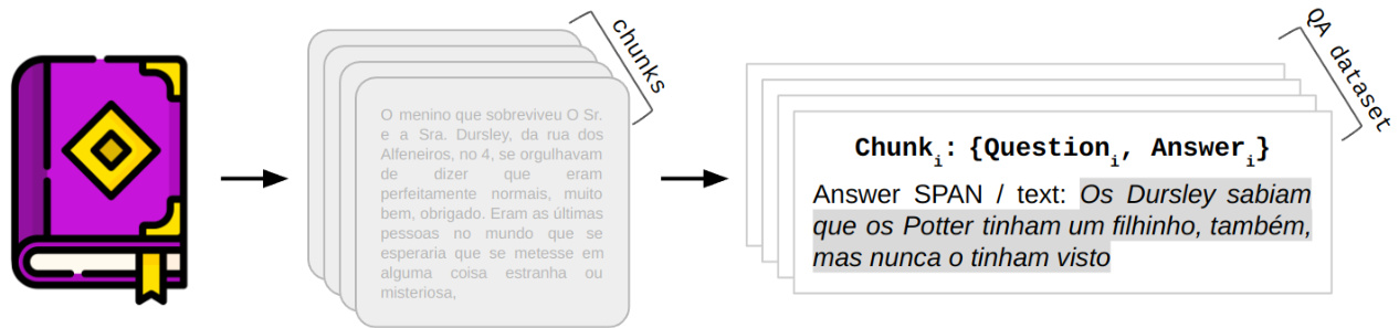
Figure 1: From a large document (book), chunks were created, and for each chunk, a question and an answer were generated using gpt-4, where the answer is contained within the chunk.
图 1: 从大型文档(如书籍)中创建文本块,并使用 gpt-4 为每个文本块生成问题和答案,其中答案包含在对应的文本块内。
Figure 1 shows the data preparation process. Initially, the dataset was break into chunks with 1000 tokens each, without overlapping, resulting in 140 chunks. Then, using the prompt described in Appendix A, a ${q u e s t i o n,a n s w e r}$ pair was created for each chunk in the style of the SQuAD dataset [6], meaning that the answer to the question is present within the reference text (chunk).
图1展示了数据准备流程。首先将数据集分割为每块1000个token的非重叠块,共生成140个数据块。随后使用附录A所述的提示模板,以SQuAD数据集[6]的风格为每个数据块创建${question, answer}$问答对,即问题的答案存在于参考文本(数据块)中。
3 How to Evaluate
3 如何评估
The contextual comparison of two text samples is not a straightforward task. For instance, despite the sentence $_ 1=$ "Brazil has won 5 FIFA World Cup titles.", and sentence $\mathrm{\Omega}_{2}=\mathrm{\Omega}^{\prime\prime}B$ razil is the five-time champion of the FIFA World Cup." (both sentences translated into English for convenience) convey the same meaning, traditional metrics such as BLEU [7] and ROUGE [8] score may not be able to capture such similarity. Specifically, for the example cited:
两个文本样本的上下文对比并非易事。例如,尽管句子 $_ 1=$ "巴西已赢得5次 FIFA 世界杯冠军" 与句子 $\mathrm{\Omega}_{2}=\mathrm{\Omega}^{\prime\prime}B$ razil is the five-time champion of the FIFA World Cup." (为方便起见均译为英文) 表达相同含义,但传统指标如 BLEU [7] 和 ROUGE [8] 可能无法捕捉此类相似性。具体到所举案例:
$$
\begin{array}{r l}&{\bullet\mathrm{\sf BLEU}\mathrm{\sf score}\left[\mathrm{sentence}_ {1},\mathrm{sentence}_ {2}\right]=0.33}\ &{\bullet\mathrm{\sf ROUGE}\mathrm{\sf score}\left[\mathrm{sentence}_ {1},\mathrm{sentence}_{2}\right]=0.22}\end{array}
$$
$$
\begin{array}{r l}&{\bullet\mathrm{\sf BLEU}\mathrm{\sf score}\left[\mathrm{sentence}_ {1},\mathrm{sentence}_ {2}\right]=0.33}\ &{\bullet\mathrm{\sf ROUGE}\mathrm{\sf score}\left[\mathrm{sentence}_ {1},\mathrm{sentence}_{2}\right]=0.22}\end{array}
$$
Therefore, an approach widely used in the literature is to employ gpt-4 to provide a score based on a given prompt, a concept similar to what was done in the G-Eval work [9]. In this work, a scoring system divided into 5 categories to compare two texts was devised, with scores defined as following (translated into English for convenience):
因此,文献中广泛采用的一种方法是利用gpt-4根据给定提示提供评分,这一思路与G-Eval研究[9]的做法类似。该研究设计了一个分为5个类别的评分系统来比较两段文本,评分标准如下(为便于理解已译为英文):
The prompt used in the evaluation is shown in Appendix A. Our approach uses a one-shot technique for each scoring category. Although, we believe that the evaluation could become more robust and deterministic with the addition of more few-shot examples for each scoring category, these possible variations were not explored in this work.
评估中使用的提示词见附录A。我们的方法对每个评分类别采用单样本(one-shot)技术。尽管我们认为通过为每个评分类别增加更多少样本示例可以使评估更具鲁棒性和确定性,但本文未探讨这些可能的变体。
3.1 Relative Maximum Score
3.1 相对最高分
In order to assess performance variation for the followings experiments, we created a metric called the relative maximum score, which corresponds to the score given by a model when evaluating the correct combination of question and chunk for all pairs of a given dataset. Through this approach, it is possible to obtain the maximum score that an evaluated LLM could reach for a RAG system.
为了评估后续实验的性能变化,我们创建了一个名为相对最高分的指标,该指标对应模型在评估给定数据集中所有问题与文本块正确组合时给出的分数。通过这种方法,可以得出被评估大语言模型在RAG系统中可能达到的最高分。
The Table 1 presents results for the custom dataset created in Section 2, by using different LLMs to generate the answer and the gpt-4 score system previously defined.
表 1: 展示了第 2 节中创建的自定义数据集结果,通过使用不同的大语言模型生成答案,并采用先前定义的 gpt-4 评分系统进行评估。
Table 1: Relative maximum score in 140 questions from the created QA Harry Potter dataset.
| Model | Relative Maximum |
| gpt-4 | 7.55 |
| gpt-4-1106-preview | 7.32 |
| gpt-3.5-turbo-1106 | 7.35 |
| Gemini Pro | 7.52 |
表 1: 自建哈利波特QA数据集中140道题的相对最高得分。
| 模型 | 相对最高分 |
|---|---|
| gpt-4 | 7.55 |
| gpt-4-1106-preview | 7.32 |
| gpt-3.5-turbo-1106 | 7.35 |
| Gemini Pro | 7.52 |
Despite configuring all the seeds and reusing the prompts, the relative maximum in our data was approximately 7.4 average points. This points out that, even with a perfect retriever strategy, the RAG system is not able to achieve a perfect score in this dataset by using these LLM models.
尽管配置了所有种子并重复使用提示词,我们数据中的相对最大值仍约为7.4个平均点。这表明,即使采用完美的检索策略,RAG系统也无法通过这些大语言模型在该数据集上获得满分。
For now on, all experiments in this study were assessed in terms of both the relative maximum and the percentage degradation with respect to the relative maximum, as defined in Equation 1.
从现在开始,本研究中的所有实验都将根据相对最大值以及与相对最大值相关的百分比退化进行评估,如公式1所定义。
$$
{\mathrm{degradation score}}=1-{\frac{\mathrm{experiment score}}{\mathrm{relative maximum}}}
$$
$$
{\mathrm{degradation score}}=1-{\frac{\mathrm{experiment score}}{\mathrm{relative maximum}}}
$$
With this score, we are able to address the problems regarding the retriever system itself, instead of having a vague idea of where is the main gap of our pipeline.
有了这个评分,我们就能解决检索系统本身的问题,而不是对整个流程的主要差距只有一个模糊的概念。
4 Introductory Experiments
4 入门实验
In this section, we will establish a baseline for the metrics defined in Section 3. Additionally, we will apply techniques of lower complexity and compare the results with the baseline. It’s worth noting that we did not explore prompt engineering techniques, although we are aware that prompt engineering has a direct impact on performance, as demonstrated in [10].
在本节中,我们将为第3节定义的指标建立基线。此外,我们将应用复杂度较低的技术,并将结果与基线进行比较。值得注意的是,我们未探索提示工程 (prompt engineering) 技术,尽管我们意识到提示工程会直接影响性能,如[10]所示。
4.1 Baseline: no context
4.1 基线:无上下文
We are aware that LLMs are trained on a massive dataset that covers virtually the entire web. This circumstance, coupled with the popularity of the Harry Potter universe, forms a robust hypothesis for testing questions in isolation on OpenAI models. The answer for basic questions such as "Who is Harry Potter?", "Who killed Dumbledore?", and "What are Harry Potter’s main friends?", ChatGPT were correctly answered with precision. However, we observed that when dealing with more detailed questions, the performance was only reasonable. Below are two examples of detailed questions (translated into English for convenience):
我们清楚大语言模型(LLM)是在覆盖几乎整个互联网的海量数据集上训练的。这一事实,加上《哈利·波特》系列的超高人气,为在OpenAI模型上独立测试问题提供了坚实假设基础。诸如"哈利·波特是谁?"、"谁杀了邓布利多?"以及"哈利·波特的主要朋友有哪些?"等基础问题,ChatGPT都能精准回答。但我们也发现,当面对更细节的问题时,模型表现只能算差强人意。以下是两个细节问题的示例(为方便理解已译成英文):
The Table 2 shows the baseline results obtained using some known LLMs for the 140 questions built as described in section 2 and evaluated as described in section 3. For this task, no retrieved context were used, only the question.
表 2 展示了使用部分已知大语言模型 (LLM) 在 140 道题目上获得的基线结果,这些题目如第 2 节所述构建,并按照第 3 节所述进行评估。在此任务中,仅使用问题本身,未使用任何检索上下文。
Table 2: Performance of the External Knowledge experiment.
| Model | AverageScore | Degradation |
| gpt-4 | 5.35 | -29.1% |
| gpt-4-1106-preview | 5.06 | -30.9% |
| gpt-3.5-turbo-1106 | 4.91 | -32.8% |
| GeminiPro | 3.81 | -50.8% |
表 2: 外部知识实验性能表现
| Model | AverageScore | Degradation |
|---|---|---|
| gpt-4 | 5.35 | -29.1% |
| gpt-4-1106-preview | 5.06 | -30.9% |
| gpt-3.5-turbo-1106 | 4.91 | -32.8% |
| GeminiPro | 3.81 | -50.8% |
4.2 Long Context
4.2 长上下文
In comparison to the GPT 1 and 2 models [11, 12], which handle up to 1024 input tokens, the gpt-4-1106-preview model stands out for its remarkable ability to process up to $128\mathrm{k\Omega}$ input tokens. This represents an approximately 128 times increase in input capacity over just four years in model development.
与GPT 1和2模型[11, 12]相比(最多处理1024个输入token), gpt-4-1106-preview模型凭借其处理高达$128\mathrm{k\Omega}$输入token的卓越能力脱颖而出。这标志着模型开发仅四年间输入容量就提升了约128倍。
The specific architecture of gpt-4 has not been disclosed, but it is believed that this model has not been pre-trained with a $128\mathrm{k\Omega}$ token input context [13]. Perhaps a post-pre-training technique could have been used, which would have made it possible to expand the number of input tokens [14, 15]. However, it is essential to note that such a technique may show degradation as the expansion limit is reached [16]. Similar to Recurrent Neural Networks (RNNs), which theoretically have an infinite context, disregarding performance limitations and vanish-gradients, we are interested in evaluating the performance of gpt-4-1106-preview over its 128k tokens.
gpt-4的具体架构尚未公开,但据信该模型并未采用128kΩ token的输入上下文进行预训练[13]。可能采用了后预训练(post-pre-training)技术,从而实现了输入token数量的扩展[14,15]。但需注意,这种技术在接近扩展极限时可能出现性能衰减[16]。与理论上具有无限上下文的循环神经网络(RNNs)类似(不考虑性能限制和梯度消失问题),我们关注的是评估gpt-4-1106-preview在其128k token长度下的表现。
To assess the impact of the gpt-4-1106-preview full context capacity on the model’s response, we proceed with a similar analysis of "Lost in The Middle" [17] in our dataset. This analysis explores the model output for a given question while changing the position of the answer throughout the prompt. To conduct this experiment, the depth of the chunk containing the answer for the question was altered in increments of $10%$ of the total number of tokens in the context’s prompt. Thus, on the y-axis, there are 11 variations of answer depth, represented by $0%$ , $10%$ , $20%,\ldots,90%$ , $100%$ , and the $\mathbf{X}$ -axis represents the quantity of tokens used as input in the context, as shown in Figure 2. The colors represents the experiment score, where the greener the better.
为评估gpt-4-1106-preview模型全上下文容量对响应的影响,我们在数据集中对"Lost in The Middle"[17]进行了类似分析。该研究通过改变答案在提示文本中的位置,观察模型对同一问题的输出变化。实验采用分块深度调整策略,以上下文总token数的$10%$为增量单位移动答案所在区块位置。纵轴显示11种答案深度变体 ($0%$、$10%$、$20%,\ldots,90%$、$100%$) ,横轴 ($\mathbf{X}$轴) 表示上下文输入的token数量,如图2所示。颜色越绿表示实验评分越高。
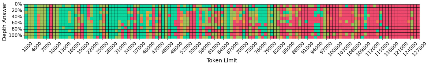
Figure 2: Performance of gpt-4-1106-preview on the Harry Potter dataset, x-axis: spaced at every $1,000$ tokens of input from the document, y-axis: represents the depth at which the answer is located in the document. The greener the better. Image based on Gregory repository [18].
图 2: gpt-4-1106-preview 在《哈利·波特》数据集上的表现,x轴: 以文档中每 $1,000$ 个token为间隔,y轴: 表示答案在文档中的深度。颜色越绿表示性能越好。图片基于 Gregory 仓库 [18]。
For instance, for $(x=100,000$ , $y=40%$ ), there are (39 chunks, followed by the chunk containing the answer, then by the remaining 60 chunks, making up the 100, 000 tokens in the input context. Based on Figure 2, we can also see when increasing the input length, we see a strong degradation in the score. Besides that, the Figure 3 shows that answers located in the interval of $(40%$ , $80%$ ) exhibit the worst performance, as documented in the article "Lost In The Middle" [17].
例如,对于 $(x=100,000$ , $y=40%$ ),输入上下文中包含 (39 个数据块,接着是包含答案的数据块,然后是剩余的 60 个数据块,共 100,000 个 token。根据图 2,我们还可以看到当输入长度增加时,分数会显著下降。此外,图 3 显示位于 $(40%$ , $80%$ ) 区间内的答案表现最差,如论文《Lost In The Middle》[17] 所述。
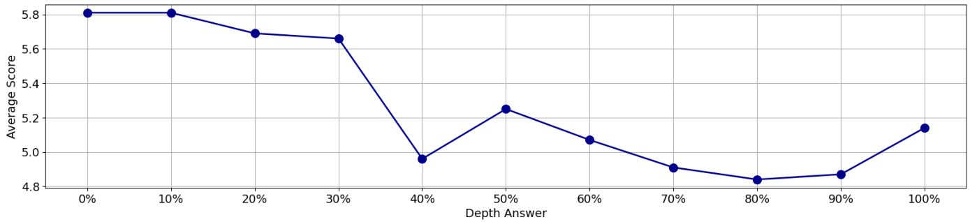
Figure 3: Average performance analysis of gpt-4-1006-preview using $128\mathrm{k\Omega}$ tokens context per answer depth.
图 3: 使用每答案深度 $128\mathrm{k\Omega}$ Token 上下文的 gpt-4-1006-preview 平均性能分析。
4.3 RAG Naive
4.3 朴素RAG
Initially, a straightforward approach for RAG will be done using the llama-index [19], employing all default hyperparameters and using chunk retrieval by cosine similarity with the ADA-002 embedding. Figure 4 depicts the basic diagram of how the problem is addressed.
最初,将使用llama-index [19]采用一种直接的RAG方法,运用所有默认超参数,并通过ADA-002嵌入的余弦相似度进行分块检索。图4展示了该问题的基本解决示意图。
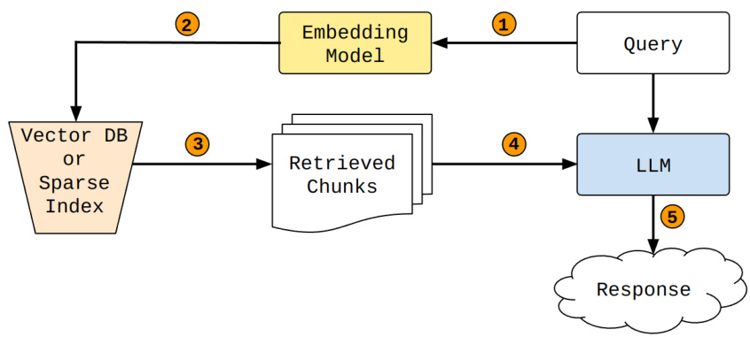
Figure 4: 1. Pass the query to the embedding model to represent its semantics as an embedded query vector; 2. Transfer the embedded query vector to vector database or sparse index (BM25); 3. Fetch the top $\boldsymbol{\cdot}\mathbf{k}$ relevant chunks, determined by retriever algorithm; 4. Forward the query text and the chunks retrieved to Large Language Model (LLM); 5. Use the LLM to produce a response based on the prompt filled by the retrieved content.
图 4: 1. 将查询传递给嵌入模型,将其语义表示为嵌入查询向量;2. 将嵌入查询向量传输到向量数据库或稀疏索引 (BM25);3. 获取前 $\boldsymbol{\cdot}\mathbf{k}$ 个相关块,由检索算法确定;4. 将查询文本和检索到的块转发给大语言模型 (LLM);5. 使用LLM基于检索内容填充的提示生成响应。
The Table 3 shows the average and degradation metrics for this approach using 2 retrieved chunks.
表 3: 展示了该方法使用2个检索块时的平均指标与退化指标。
Table 3: Performance of the RAG naive.
| Model | Average Score | Degradation |
| gpt-4 | 6.04 | -20% |
| gpt-4-1106-preview | 5.74 | -21.6% |
| gpt-3.5-turbo-1106 | 5.80 | -21.0% |
表 3: RAG naive 的性能表现
| 模型 | 平均得分 | 性能下降 |
|---|---|---|
| gpt-4 | 6.04 | -20% |
| gpt-4-1106-preview | 5.74 | -21.6% |
| gpt-3.5-turbo-1106 | 5.80 | -21.0% |
5 Advanced Experiments
5 进阶实验
The studies and experiments outlined in section 4 have shown unsatisfactory performance, marked by a degradation of at least $20%$ compared to the peak relative performance. Therefore, in this section, we explore various retrieval approaches for the RAG, recognizing that the quality of the retriever is a crucial factor in enhancing performance for this type of problem. We conducted an evaluation covering both sparse and dense search, a hybrid method, and even a multi-stage architecture using a reranker.
第4节所述的研究和实验显示出不理想的性能,其相对峰值性能至少下降了20%。因此,本节我们探索了多种RAG检索方法,认识到检索器质量是提升此类问题性能的关键因素。我们评估了稀疏搜索、密集搜索、混合方法,甚至采用了重排序器的多阶段架构。
In pursuit of code debugging flexibility and easier customization at each stage, we chose not to utilize an RAG framework (like LangChain or Llama-Index). For a comprehensive guide on debugging RAG and more details about retrieval systems, refer to [20] and [21].
为了追求代码调试的灵活性和各阶段更易定制化,我们选择不使用RAG框架(如LangChain或Llama-Index)。关于RAG调试的完整指南及检索系统的更多细节,请参阅[20]和[21]。
5.1 Retrievers
5.1 检索器
When deploying retrieval systems, it is essential to achieve a balance between “effectiveness” (How good are the results returned?) and “efficiency” (How much time it takes to return the results? or How much resources are used in terms of disk/RAM/GPU?). This balance ensures that latency, result quality, and computational budget remain within our application’s required limits. This work will exclusively focus on effectiveness measures to quantify the retrievers methods quality.
在部署检索系统时,必须在"效果"(返回的结果质量如何?)和"效率"(返回结果需要多长时间?或消耗多少磁盘/RAM/GPU资源?)之间取得平衡。这种平衡确保延迟、结果质量和计算预算保持在应用要求的范围内。本文工作将仅关注量化检索方法质量的效能指标。
In our retriever experiments, the evaluation strategy centers around assessing how well the retriever performs in retrieving relevant information based on each given query $q_{i}$ . To achieve this, we employ the concept of recall. It is defined as the fraction of the relevant documents for a given query $q_{i}$ that are successfully retrieved in a ranked list $R$ [21]. This metric is based on binary relevance judgments, assuming that documents are either relevant or not [21]. In this paper, each chunk is considered a document and only the respective chunk $d_{i}$ is considered relevant to the query $q_{i}$ . While recall is easy to interpret, it does not consider the specific rank positions in which the relevant chunk appears in $R$ .
在我们的检索器实验中,评估策略的核心是衡量检索器根据每个给定查询$q_{i}$检索相关信息的效果。为此,我们采用了召回率(recall)的概念。其定义为:在排序列表$R$中成功检索到的与查询$q_{i}$相关文档的比例[21]。该指标基于二元相关性判断,假设文档要么相关要么不相关[21]。本文中,每个文本块被视为一个文档,且仅将对应块$d_{i}$视为与查询$q_{i}$相关。虽然召回率易于解释,但它不考虑相关块在$R$中出现的具体排名位置。
To overcome this limitation, we introduce Reciprocal Rank (RR) into our analysis. In this metric, the rank of the first relevant document to the query in $R$ is used to compute the RR score [21]. Therefore, Reciprocal Rank offers a more nuanced evaluation by assigning a higher value when the relevant chunk is returned in the early positions of our retrievers given the respective query.
为克服这一局限,我们在分析中引入了倒数排名 (Reciprocal Rank, RR) 指标。该指标通过计算查询结果集 $R$ 中首个相关文档的排名来得出RR分数 [21]。因此,当相关文本块在检索结果的前列位置返回时,倒数排名能通过赋予更高分值来实现更精细的评估。
Recall and Reciprocal Rank were evaluated at a specific cutoff so the measures are presented as $\mathbf R\ @\mathbf K$ and MRR $\ @\mathbf{k}$ . For each query, its results are evaluated and their mean serves as an aggregated measure of effectiveness of a given retriever method. The retrievers are introduced below.
在特定截断点评估召回率 (Recall) 和倒数排名 (Reciprocal Rank),因此指标表示为 $\mathbf R\ @\mathbf K$ 和 MRR $\ @\mathbf{k}$。每个查询的结果经过评估后,其均值作为给定检索方法效果的综合衡量指标。检索器介绍如下。
In the category of sparse retrievers, we emphasize the BM25, a technique grounded in statistical weighting to assess relevance between search terms and documents. BM25 employs a scoring function that takes into account term frequency and document length, offering an efficient approach for retrieving pertinent information and is typically used as a strong baseline. However, it is exact-match based and can be powerless when query and document are relevant to each other but has no common words.
在稀疏检索器类别中,我们重点介绍BM25,这是一种基于统计加权来评估搜索词与文档相关性的技术。BM25采用了一个考虑词频和文档长度的评分函数,为检索相关信息提供了一种高效方法,通常被用作强有力的基线。然而,它基于精确匹配,当查询和文档彼此相关但没有共同词汇时,可能会无能为力。
On the other hand, when exploring dense retrievers, we often encounter approaches based on the called bi-encoder design [22]. The bi-encoder independently encodes queries and documents, creating separate vector representations before calculating similarity. An advantage of this approach is that it can be initialized ‘offline’: document embeddings can be pre computed, leaving only the query embedding being calculated at search time, reducing latency.
另一方面,在探索密集检索器时,我们经常会遇到基于双编码器设计 (bi-encoder) [22] 的方法。双编码器独立编码查询和文档,在计算相似度前创建独立的向量表示。这种方法的优势在于可以"离线"初始化:文档嵌入可以预先计算,仅需在搜索时计算查询嵌入,从而降低延迟。
The hybrid search technique aims to leverage the best of both sparse and dense search approaches. Given a question, both searches are conducted in parallel, generating two lists of candidate documents to answer it. The challenge then lies in combining the two results in the best possible way, ensuring that the final hybrid list surpasses the individual searches. Essentially, we can conceptualize it as a voting system, where each searcher casts a vote on the relevance of a document to a given query, and in the end, the opinions are combined to produce a better result.
混合搜索技术旨在结合稀疏搜索和密集搜索方法的优势。给定一个问题时,会并行执行两种搜索,生成两份候选文档列表来回答该问题。随后面临的挑战在于以最佳方式合并这两个结果,确保最终的混合列表优于单独的搜索结果。从本质上讲,可以将其概念化为一个投票系统:每个搜索器对文档与查询的相关性进行投票,最终通过综合意见得出更优的结果。
The multi-stage search architecture is based on the retrieve-and-rerank pipeline. In the first stage, a retriever with good recall is typically used to perform an initial filtering of the documents to be returned. From this narrowed-down list, these candidate documents are then sent to a second stage, which involves higher computational complexity, to rerank them and enhance the final effectiveness of the system.
多阶段搜索架构基于检索-重排序流程。在第一阶段,通常使用具有高召回率的检索器对返回文档进行初步筛选。从这份缩减后的候选列表中,这些文档会被送入计算复杂度更高的第二阶段进行重排序,以提升系统的最终效果。
Next, we provide more details about each retriever used.
接下来,我们将详细介绍所使用的每个检索器。
5.1.1 BM25
5.1.1 BM25
Due to the user-friendly nature of BM25, its inclusion as a retriever method is always a welcome addition in RAG evaluations. A study that aligns with the same reasoning, albeit for a different application, can be found in [23], which illustrates the benefits of employing this algorithm to establish a robust baseline. Given that our data shares similarities with the ${\tt S Q u A D}$ dataset, it is expected that many words from the query would be present in the chunk, contributing to the favorable effectiveness of BM25.
由于BM25具有用户友好的特性,在RAG评估中将其作为检索方法始终是受欢迎的补充。一项遵循相同思路的研究(尽管针对不同应用)可参见[23],该研究阐述了使用该算法建立稳健基线的优势。鉴于我们的数据与${\tt S Q u A D}$数据集具有相似性,预计查询中的许多词会出现在文本块中,从而提升BM25的良好效果。
In the BM25 ranking function, $k_{1}$ and $b$ are parameters shaping term saturation and document length normalization, respectively. The BM25 formula integrates these parameters to score the relevance of a document to a query, offering flexibility in adjusting $k_{1}$ and $b$ for improving effectiveness in different retrieval scenarios.
在BM25排序函数中,$k_{1}$和$b$分别是控制词项饱和度和文档长度归一化的参数。BM25公式通过整合这些参数来计算文档与查询的相关性得分,并提供了调整$k_{1}$和$b$的灵活性,以提升不同检索场景下的效果。
Table 4: Comparison between BM25 packages using $_{\mathrm{k}1=0.82}$ and $\scriptstyle=0.68$
| Recall@k | rank-bm25 | Pyserini BM25 | Pyserini Gain (%) |
| 3 | 0.735 | 0.914 | 24.3 |
| 5 | 0.814 | 0.971 | 19.2 |
| 7 | 0.857 | 0.985 | 14.9 |
| 9 | 0.878 | 0.985 | 12.1 |
表 4: 使用 $_{\mathrm{k}1=0.82}$ 和 $\scriptstyle=0.68$ 的 BM25 包对比
| Recall@k | rank-bm25 | Pyserini BM25 | Pyserini Gain (%) |
|---|---|---|---|
| 3 | 0.735 | 0.914 | 24.3 |
| 5 | 0.814 | 0.971 | 19.2 |
| 7 | 0.857 | 0.985 | 14.9 |
| 9 | 0.878 | 0.985 | 12.1 |
Effectiveness is also influenced by chosen BM25 implementation. Pyserini’s BM25 implementation incorporates an analyzer with preprocessing steps such as stemming and language-specific stop word removal. For the sake of comparison, we included results obtained using rank-bm25 [24], a basic implementation without preprocessing that is widely used in Python and integrated into libraries like LangChain and Llama-index. The results can be seen in Table 4.
效果还受所选BM25实现的影响。Pyserini的BM25实现包含一个分析器,具有词干提取和特定语言停用词移除等预处理步骤。为了比较,我们加入了使用rank-bm25 [24]获得的结果,这是一个没有预处理的基础实现,广泛用于Python语言并集成到LangChain和Llama-index等库中。结果如表4所示。
In this work, the Pyserini BM25 implementation [25] was used in all experiments considering $k_{1}=0.82$ and $\scriptstyle{b=0.68}$ .
在本工作中,所有实验均采用Pyserini BM25实现[25],参数设置为 $k_{1}=0.82$ 和 $\scriptstyle{b=0.68}$。
5.1.2 ADA-002
5.1.2 ADA-002
OpenAI does not disclose extensive details about the ADA-002 architecture; however, we employed this model in retrieval as the presented bi-encoder design (Figure 5): vector representations were constructed for all available chunks, and for each input query, its embedding was computed at search time. Subsequently, the similarity between the question and chunk were assessed using cosine similarity.
OpenAI并未公开ADA-002架构的详细设计,但我们采用该模型实现了双编码器检索方案(图5):为所有文本块生成向量表征,并在搜索时实时计算输入查询的嵌入向量,最后通过余弦相似度评估问题与文本块的相关性。
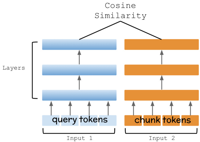
Figure 5: Bi-Encoder Architecture
图 5: 双编码器架构
Since we have no further details about ADA-002 we will refer to this approach only as dense retriever.
由于我们无法获得ADA-002的更多细节,因此仅将这种方法称为密集检索器 (dense retriever)。
5.1.3 Custom ADA-002
5.1.3 自定义ADA-002
Embedding customization is not limited solely to OpenAI’s embeddings; it is a technique applicable to other embeddings of the same kind. There is a significant variety of approaches to optimize a matrix, with one of them being the application of Multiple Negative Ranking Loss, as presented in the article "Efficient Natural Language Response Suggestion for Smart Reply," Section 4.4 [26]. However, given our current focus on simplicity, we will reserve the exploration of this technique for future work. At this moment, we choose to utilize the Mean Squared Error (MSE) Loss.
嵌入定制不仅限于OpenAI的嵌入技术,它同样适用于同类其他嵌入方法。优化矩阵的方法多种多样,其中一种如论文《智能回复的高效自然语言响应建议》第4.4节[26]所述,可采用多重负样本排序损失(Multiple Negative Ranking Loss)。但鉴于当前我们追求简洁性,该技术的探索将留待后续研究。现阶段我们选择使用均方误差损失(MSE Loss)。
For the fine-tuning stage, it is necessary to have two types of samples:
在微调阶段,需要准备两类样本:
$\bullet\mathrm{positives:}[\mathrm{question}_ {i},\mathrm{chunk}_{i},l a b e l=1]$ negatives: [questioni, chunkj, $l a b e l=-1]$ , for $i\neq j$
$\bullet\mathrm{正例:}[\mathrm{问题}_ {i},\mathrm{片段}_{i},标签=1]$ 负例: [问题i, 片段j, $标签=-1]$ , 当 $i\neq j$
Often, as is the case with our dataset, only positive examples are available. However, through a simple and random shuffling, it is possible to generate negative examples. Demonstrating confidence in transfer learning, we found that a few examples were sufficient. Our final dataset consisted of approximately 400 examples, maintaining a $1:3$ ratio between positive and negative examples.
通常,就像我们的数据集一样,只有正样本可用。但通过简单随机打乱,可以生成负样本。基于对迁移学习的信心,我们发现少量样本就已足够。最终数据集包含约400个样本,正负样本比例保持在$1:3$。
The hyper parameters that exert the most significant impact on performance include the learning rate, batch size, and the number of dimensions in the projection matrix. The ADA-002 model has 1536 dimensions, and the projection matrix is of size $1536\times\mathrm{N}$ , where N ∈ 1024, 2048, 4096. In our experiments, we observed that 2048 dimensions resulted in the best accuracy.
对性能影响最显著的超参数包括学习率、批量大小和投影矩阵的维度数。ADA-002模型具有1536个维度,其投影矩阵尺寸为$1536\times\mathrm{N}$,其中N ∈ 1024, 2048, 4096。实验表明2048维度能获得最佳准确率。
This type of fine-tuning requires low GPU resources, with a training time of approximately 5 minutes using the A100 GPU. The model itself is straightforward, consisting of a matrix with dropout (to mitigate over fitting), followed by the hyperbolic tangent activation function, which provided additional accuracy gains in the training set.
此类微调对GPU资源需求较低,使用A100 GPU时训练时间约为5分钟。该模型结构简洁,包含一个带dropout(用于防止过拟合)的矩阵,后接双曲正切激活函数,该设计在训练集上带来了额外的准确率提升。
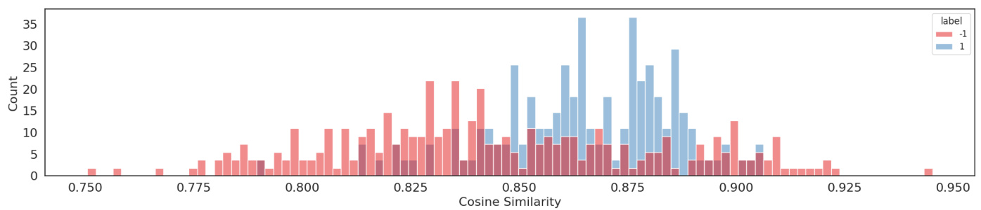
Figure 6: Cosine similarity of positive and negative classes in the ADA-002 embedding; note the significant overlap between the classes. Test accuracy (before training): $69.5%$
图 6: ADA-002嵌入中正负类别的余弦相似度;注意类别间存在显著重叠。测试准确率(训练前): $69.5%$
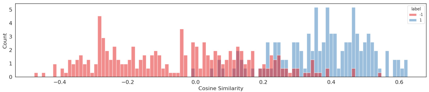
Figure 7: Cosine similarity of positive and negative classes in the customized embedding; the intersection between the classes is minimal. Test accuracy (after training): $84.3%$
图 7: 定制化嵌入中正负类别的余弦相似度;类别间交集极小。测试准确率(训练后): $84.3%$
When analyzing the cosine similarity between positive and negative classes, we can observe the "shadow" shared by the histograms. In an ideal scenario, we desire the classes to be disjoint to ensure a clear definition of space. Figure 6 illustrates a significant shadow in the embedding before training, while Figure 7 shows the result after training. Both graphs are derived from the test set. Test accuracy also improved, leading to a better dense representation.
在分析正负类之间的余弦相似度时,我们可以观察到直方图共有的"阴影"。理想情况下,我们希望各类别互不相交以确保空间定义的清晰性。图6展示了训练前嵌入中存在显著阴影,而图7则显示了训练后的结果。两张图表均来自测试集。测试准确率也有所提升,从而获得了更好的密集表示。
5.1.4 Hybrid Search
5.1.4 混合搜索
As stated before, hybrid search is applied when is necessary to combine results from two or more retrieval methods. A widely used algorithm to address this type of problem is known as Reciprocal Rank Fusion (RRF). For a document
如前所述,混合搜索 (hybrid search) 用于需要整合两种或以上检索方法结果的场景。解决此类问题的常用算法称为逆序融合排序 (Reciprocal Rank Fusion, RRF)。对于文档
set $D$ and search results from different methods $r$ in $R$ , for each $d$ in $D$ , we can calculate the $R R F_{s c o r e}(d\in D)$ as follows [27]:
对于集合 $D$ 和不同方法的搜索结果 $r$ 属于 $R$,针对每个 $d$ 在 $D$ 中,我们可以计算 $R R F_{s c o r e}(d\in D)$ 如下[27]:
$$
R R F_{s c o r e}(d\in D)=\sum_{r\in R}\frac{1}{k+r(d)},
$$
$$
R R F_{s c o r e}(d\in D)=\sum_{r\in R}\frac{1}{k+r(d)},
$$
Considering that $1/r(d)$ is known as the reciprocal rank, where $r(d)$ represents the position at which the document $d$ was retrieved by the search mechanism $r$ . The term $k$ is introduced to assist in controlling outlier systems [27].
考虑到 $1/r(d)$ 被称为倒数排名 (reciprocal rank),其中 $r(d)$ 表示文档 $d$ 被搜索机制 $r$ 检索到的位置。引入参数 $k$ 是为了帮助控制异常系统 [27]。

Figure 8: Hybrid Search schema with $\mathrm{k}{=}1$ .
图 8: 混合搜索方案 (Hybrid Search schema) 其中 $\mathrm{k}{=}1$。
Figure 8 shows how to calculate $R R F_{s c o r e}$ for $k=1$ . In the example, we have four chunks that were retrieved in different orders by two search methods, BM25 (sparse search), and Custom ADA-002 (dense search). The reciprocal rank score is calculated for each chunk. These values are then summed, creating a new score. The final hybrid list is an ordering of chunks that uses this new score.
图 8: 展示了如何计算 $k=1$ 时的 $R R F_{s c o r e}$。示例中包含四个文本块,它们分别被两种搜索方法 BM25 (稀疏搜索) 和 Custom ADA-002 (稠密搜索) 以不同顺序检索出来。每个文本块都会计算其倒数排名得分,随后将这些值相加生成新得分。最终的混合列表就是根据这个新得分对文本块进行排序的结果。
Table 5: Retriever comparison. Where MRR is the Mean Re cri pro cal Rank metric and $\mathbf R\ @\mathbf K$ is the Recall.
| Metric | Hybrid-BM25-ADA-002 | Hybrid-BM25-Custom ADA-002 |
| MRR@10 | 0.758 | 0.850 |
| R@3 | 0.829 | 0.921 |
| R@5 | 0.879 | 0.943 |
| R@7 | 0.921 | 0.964 |
| R@9 | 0.957 | 0.979 |
表 5: 检索器对比。其中 MRR 表示平均倒数排名 (Mean Reciprocal Rank) 指标,$\mathbf R\ @\mathbf K$ 表示召回率 (Recall)。
| 指标 | Hybrid-BM25-ADA-002 | Hybrid-BM25-Custom ADA-002 |
|---|---|---|
| MRR@10 | 0.758 | 0.850 |
| R@3 | 0.829 | 0.921 |
| R@5 | 0.879 | 0.943 |
| R@7 | 0.921 | 0.964 |
| R@9 | 0.957 | 0.979 |
In our experiments, only Pyserini’s BM25 was tested as the sparse retriever, while ADA-002 and Custom ADA-002 were tested as dense retrievers. The hybrid combination that yielded the best results was the one that used BM25 and Custom ADA-002.
在我们的实验中,仅测试了Pyserini的BM25作为稀疏检索器,而ADA-002和Custom ADA-002作为稠密检索器进行了测试。效果最佳的混合组合是使用了BM25和Custom ADA-002的方案。
5.1.5 Reranker
5.1.5 重排序器
The fundamental idea underlying multi-stage ranking is to divide document ranking into a sequence of stages. After an initial retrieval, which usually involves a sparse retriever or dense retriever, each subsequent stage re-evaluates and reranks the set of candidates forwarded from the preceding stage. Figure 9 represents a multi-stage pipeline where Pyserini BM25 performs the first stage and the candidate chunks are then re-evaluated by the reranker. After that, the final reranked list called retrieved chunks is presented as final result formed by $k$ chunks.
多阶段排序的基本思想是将文档排序划分为一系列阶段。在初始检索(通常涉及稀疏检索器或密集检索器)之后,每个后续阶段会对前序阶段传递的候选集进行重新评估和重排序。图9展示了一个多阶段流程:Pyserini BM25执行第一阶段检索,随后由重排序器对候选文本块进行重新评估。最终形成的重排序列表(称为检索文本块)将呈现为由$k$个文本块构成的最终结果。

Figure 9: Reranker Pipeline
图 9: 重排序流程
Transformers-based models are commonly employed as rerankers, leveraging their capability to enhance the effectiveness of information retrieval systems by capturing intricate relationships and contextual information within documents and queries.
基于Transformer的模型通常被用作重排序器,利用其捕获文档和查询中复杂关系及上下文信息的能力,提升信息检索系统的有效性。
The initial utilization of transformers within a multi-stage ranking framework was presented in the study [28]. Their proposed model, known as monoBERT, transforms the ranking process into a relevance classification problem. It achieves this by sorting texts based on the conditional probability $P({\mathrm{Relevant}}=1|d_{i};q)$ , where $q$ is the query and $d_{i}$ represents documents [21]. The model simultaneously processes both queries and documents. This simultaneous processing leads to a more enriched interaction between them, often resulting in improved effectiveness [29], [30]. However, this neural models have a substantial number of parameters and the scoring of query-document pairs occurs at inference time. This, in turn, increases computational costs and latency. This kind of model is also known by cross-encoder. Refer to Figure 10 for an illustration of the query-document pair processing.
研究[28]首次提出了在多阶段排序框架中使用Transformer的方法。他们提出的模型monoBERT将排序过程转化为相关性分类问题,通过基于条件概率$P({\mathrm{Relevant}}=1|d_{i};q)$对文本进行排序实现,其中$q$表示查询,$d_{i}$代表文档[21]。该模型能同时处理查询和文档,这种并行处理方式使两者间产生更丰富的交互,通常能提升效果[29][30]。然而这类神经模型参数量庞大,且需要在推理时对查询-文档对进行评分,这会导致计算成本和延迟上升。此类模型也被称为交叉编码器(cross-encoder),查询-文档对的处理流程可参见图10。

Figure 10: Cross-Encoder
图 10: Cross-Encoder
In the other hand, monoT5 is a sequence-to-sequence reranker [31] that uses T5 models [32] to generate relevance scores between a pair of query and document. T5 models treat all tasks as text-to-text, requiring some adaptations for the query/document similarity task. During training, the format 'Query: {query} Document: {document} Relevant:' is used, with labels yes if the document is relevant to the query, and no otherwise. At inference time, the same format as the training data is used to format pairs of queries and documents to feed the model, and a single-token greedy decode is performed. The score is then obtained by calculating the softmax value considering only the tokens no and yes, and selecting the value corresponding to the yes token. Note that the tokens no and yes are the tokens used in the version provided by [33], but the publication that introduced the monoT5 architecture, [31], uses the tokens false and true. Figure 11 contains an illustration of the monoT5 architecture’s inference process.
另一方面,monoT5是一种序列到序列的重排序器 [31],它使用T5模型 [32] 来生成查询和文档之间的相关性分数。T5模型将所有任务视为文本到文本的转换,因此需要对查询/文档相似性任务进行一些调整。在训练过程中,使用格式"Query: {query} Document: {document} Relevant:",如果文档与查询相关,则标签为yes,否则为no。在推理时,使用与训练数据相同的格式来格式化查询和文档对,并执行单token贪婪解码。然后通过仅考虑no和yes token计算softmax值,并选择对应于yes token的值来获得分数。需要注意的是,no和yes token是[33]提供的版本中使用的token,但介绍monoT5架构的论文[31]使用的是false和true token。图11展示了monoT5架构的推理过程。

Figure 11: monoT5’s inference process
图 11: monoT5的推理过程
In our experiments, Pyserini BM25 was employed as first-stage retrieval, retrieving 50 documents to be reranked in the second stage. In the second stage, we utilized the model unicamp-dl/ $\mathtt{m t5}$ -base-en-pt-msmarco-v2, a sequenceto-sequence reranker trained on pairs of queries and documents in English and Portuguese from the dataset [33].
在我们的实验中,Pyserini BM25 被用作第一阶段检索,检索出 50 份文档供第二阶段重排序。在第二阶段,我们使用了模型 unicamp-dl/$\mathtt{m t5}$-base-en-pt-msmarco-v2,这是一个基于序列到序列的重排序器,训练数据来自数据集 [33] 中的英语和葡萄牙语查询-文档对。
5.2 Retrievers Results
5.2 检索器结果
The results achieved with the various retrievers are presented in Table 6.
表 6: 展示了使用不同检索器获得的结果。
Table 6: Retriever comparison.
| Metric | ADA-002 | CustomADA-002 | Hybrid-BM25-ADA-002 | Hybrid-BM25-CustomADA-002 | BM25 | BM25+Reranker |
| MRR@10 | 0.565 | 0.665 | 0.758 | 0.850 | 0.879 | 0.919 |
| R@3 | 0.628 | 0.735 | 0.829 | 0.921 | 0.914 | 0.971 |
| R@5 | 0.692 | 0.835 | 0.879 | 0.943 | 0.971 | 0.985 |
| R@7 | 0.750 | 0.871 | 0.921 | 0.964 | 0.985 | 0.992 |
| R@9 | 0.814 | 0.921 | 0.957 | 0.979 | 0.985 | 1 |
表 6: 检索器性能对比
| 指标 | ADA-002 | CustomADA-002 | Hybrid-BM25-ADA-002 | Hybrid-BM25-CustomADA-002 | BM25 | BM25+Reranker |
|---|---|---|---|---|---|---|
| MRR@10 | 0.565 | 0.665 | 0.758 | 0.850 | 0.879 | 0.919 |
| R@3 | 0.628 | 0.735 | 0.829 | 0.921 | 0.914 | 0.971 |
| R@5 | 0.692 | 0.835 | 0.879 | 0.943 | 0.971 | 0.985 |
| R@7 | 0.750 | 0.871 | 0.921 | 0.964 | 0.985 | 0.992 |
| R@9 | 0.814 | 0.921 | 0.957 | 0.979 | 0.985 | 1 |
The multi-stage pipeline was able to achieve the best results in MRR $@10$ and Recall $\ @\mathbf{k}$ .
多阶段流水线在MRR $@10$ 和召回率 $\ @\mathbf{k}$ 上取得了最佳结果。
6 Conclusions
6 结论
The implementation of RAG systems faces challenges such as the effective integration of retrieval models, efficient representation learning, the diversity of data, the optimization of computational efficiency, evaluation, and text generation quality. Faced with these constantly evolving obstacles, this article proposes best practices for the implementation, optimization, and evaluation of RAG on a Brazilian Portuguese dataset, focusing on a simplified pipeline for inference and experimentation.
RAG系统的实施面临检索模型有效集成、高效表征学习、数据多样性、计算效率优化、评估及文本生成质量等挑战。针对这些不断演变的障碍,本文提出在巴西葡萄牙语数据集上实施、优化和评估RAG的最佳实践,重点关注简化的推理和实验流程。
So far, we have introduced the main components and methods along with their results and gaps. In this section, we will discuss key points that contribute to the performance improvement in RAG applications. We will start by discussing the relationship between the quality of the retriever and the achieved performance, in which our approach showed a significant improvement of MRR $@10$ by $35.4%$ compared to the baseline. Next, we will address the impact of input size on performance. In this domain, we observed that it is possible to enhance the best information retrieval strategy by $2.\dot{4}%$ through input size optimization. Finally, we will present the complete architecture of RAG with our recommendations. When evaluating the final accuracy of our approach, we reached $98.61%$ , representing an improvement of 40.73 in less degradation score compared to the baseline.
截至目前,我们已经介绍了主要组件、方法及其结果与不足。本节将探讨提升RAG (Retrieval-Augmented Generation) 应用性能的关键因素。首先分析检索器质量与性能的关系,我们的方法相比基线在MRR$@10$上实现了35.4%的显著提升。接着讨论输入规模对性能的影响,该领域研究表明通过优化输入规模可将最佳信息检索策略提升2.$\dot{4}$%。最后展示完整RAG架构及我们的优化建议。在最终准确率评估中,我们的方法达到98.61%,相比基线在退化分数上改善了40.73分。
6.1 Retriever Score versus Performance
6.1 检索器评分与性能对比
As mentioned in section 5.1, the performance of information/chunk retrieval, measured by the $\mathrm{MRR}@10$ metric, varies between (0.565, 0.919), as detailed in Table 6. This variation represents approximately $35.4%$ . It is important to highlight that the RAG’s performance is directly influenced by the quality of the retriever. Figure 12 shows the relationship between the retrieval metric MRR $@10$ metric and the degradation score for the studied retrieval methods.
如第5.1节所述,信息/块检索性能(以$\mathrm{MRR}@10$指标衡量)在(0.565, 0.919)区间波动,具体数据见表6。该波动幅度约为$35.4%$。需要强调的是,RAG的性能直接受检索器质量影响。图12展示了所研究检索方法的MRR $@10$指标与退化分数之间的关系。

Figure 12: Retriever effectiveness vs RAG Performance. $x$ axis is the MRR $@10$ metric and $y$ axis is the degradation (where 0 is the perfect scenario) score.
图 12: 检索器效果与RAG性能对比。$x$轴表示MRR $@10$指标,$y$轴表示性能下降(0为理想情况)得分。
6.2 Input Size versus Performance
6.2 输入规模与性能
We observed that the best performance was achieved with the retrieval of 3 chunks using the retrieve-and-rerank strategy, as shown in Table 7. The use of a reranker (Figure 9) showed improved information retrieval in our tests. With this same configuration, the Gemini Pro achieved performance similar to gpt-4, as indicated in Table 8.
我们观察到,如表7所示,使用检索-重排(retrieve-and-rerank)策略检索3个文本块时获得了最佳性能。测试表明,使用重排器(图9)改善了信息检索效果。在相同配置下,Gemini Pro取得了与gpt-4相近的性能,如表8所示。
Despite achieving perfect recall for 9 chunks, as evidenced in Table 6, using an input with 9000 tokens, 6000 more than the best scenario (3 chunks), did not result in the best performance. As discussed in Section 4.2, the quality of
尽管如表 6 所示,在输入 9000 个 token (比最佳场景多 6000 个 token) 时实现了对 9 个数据块的完美召回,但并未获得最佳性能。如第 4.2 节所述,...
Table 7: Performance of number of chunks retrieved with gpt-4.
| #RetrievedChunks | ADA-002 | CustomADA-002 | BM25 | Hybrid | BM25+Reranker |
| 3 | 6.19 | 6.41 | 7.10 | 7.31 | 7.44 |
| 5 | 6.29 | 6.61 | 7.32 | 7.37 | 7.43 |
| 7 | 6.42 | 6.82 | 7.17 | 7.20 | 7.32 |
| 9 | 6.57 | 6.88 | 7.22 | 7.34 | 7.37 |
表 7: 使用 gpt-4 检索不同数量文本块时的性能表现
| #RetrievedChunks | ADA-002 | CustomADA-002 | BM25 | Hybrid | BM25+Reranker |
|---|---|---|---|---|---|
| 3 | 6.19 | 6.41 | 7.10 | 7.31 | 7.44 |
| 5 | 6.29 | 6.61 | 7.32 | 7.37 | 7.43 |
| 7 | 6.42 | 6.82 | 7.17 | 7.20 | 7.32 |
| 9 | 6.57 | 6.88 | 7.22 | 7.34 | 7.37 |
Table 8: Performance of best retriever RAG.
| Model | RetrieverMethod | #Retrieved [Chunks | Degradation |
| gpt-4 | ADA-002 | 9 | -13.0% |
| gpt-4 | ADA-002Custom | 9 | -8.8% |
| gpt-4 | BM25 | 5 | -3% |
| gpt-4 | Hybrid | 5 | -2.3% |
| gpt-4 | BM25+Reranker | 3 | -1.4% |
| GeminiPro | BM25+Reranker | 3 | -2.2% |
表 8: 最佳检索器 RAG 性能表现
| Model | RetrieverMethod | #Retrieved [Chunks | Degradation |
|---|---|---|---|
| gpt-4 | ADA-002 | 9 | -13.0% |
| gpt-4 | ADA-002Custom | 9 | -8.8% |
| gpt-4 | BM25 | 5 | -3% |
| gpt-4 | Hybrid | 5 | -2.3% |
| gpt-4 | BM25+Reranker | 3 | -1.4% |
| GeminiPro | BM25+Reranker | 3 | -2.2% |
RAG is directly related to the input size and the position where the answer is located. Therefore, the final results confirm the observations made in our experiments.
RAG与输入大小和答案所在位置直接相关。因此,最终结果证实了我们实验中的观察结果。
Moreover, from a cost perspective, it is crucial to avoid overloading the LLM with a large number of input tokens, as the cost is also based on the amount of input text.
此外,从成本角度来看,避免向大语言模型 (LLM) 输入过多 token 至关重要,因为成本也取决于输入文本的数量。
It is important to note that the results obtained in this study cannot be considered as a generalization for other datasets. Exploratory Data Analysis and the use of good retriever practices, as presented in [34], are always a solid path to achieving good results.
需要注意的是,本研究所得结果不能推广到其他数据集。探索性数据分析 (Exploratory Data Analysis) 和采用[34]中提出的优秀检索实践,始终是获得良好结果的可靠途径。
6.3 Final Results
6.3 最终结果
Despite this work being grounded in a single dataset, it is always crucial to emphasize the importance of data quality. In a simplified manner, as illustrated in Figure 13, data quality in RAG can be divided into Input, Retriever, and Evaluation.
尽管这项工作基于单一数据集,但始终需要强调数据质量的重要性。简而言之,如图13所示,RAG中的数据质量可分为输入(Input)、检索器(Retriever)和评估(Evaluation)三个部分。

Figure 13: Core Points in RAG.
图 13: RAG核心要点
• Input: How are the queries formulated? Are they synthetic or generic? What is the application’s purpose? Building a RAG for a chatbot differs significantly from constructing a RAG for extracting information from a long and complex document. • Retriever: How do the data behave in information retrieval? Are the queries strongly linked by keywords in the text? What is the cosine similarity of query-to-query, query-to-document, and document-to-document? • Evaluation: How are the data measured? Defining metrics and success rates, as in the first experiment, is always a safe path to avoid biases. Build the evaluation system before testing, avoiding bias.
• 输入:查询是如何构建的?是合成查询还是通用查询?应用目的是什么?为聊天机器人构建RAG与为从长而复杂的文档中提取信息构建RAG存在显著差异。
• 检索器:数据在信息检索中表现如何?查询是否通过文本中的关键词紧密关联?查询间、查询与文档间、文档间的余弦相似度是多少?
• 评估:如何衡量数据?如第一个实验那样定义指标和成功率,始终是避免偏差的安全路径。在测试前建立评估系统,避免偏差。
In conclusion, the main contribution of this work was to identify and present the best possible configuration of techniques and parameters for a RAG application. Figure 14 provides a summarized overview of the end-to-end experiment results for the discussed approaches, and the best practices recommended by this study achieve a final accuracy of $98.61%$ , representing an improvement of 40.73 percentage points compared to the baseline.
总之,这项工作的主要贡献是确定并呈现了RAG应用的最佳技术配置和参数组合。图14总结了所讨论方法的端到端实验结果,本研究所推荐的最佳实践实现了98.61%的最终准确率,相比基线提升了40.73个百分点。

Figure 14: RAG Performance: Performance evolution on the Harry Potter dataset, where an accuracy of $100%$ is considered the relative maximum.
图 14: RAG性能: 在《哈利·波特》数据集上的性能演变,其中 $100%$ 准确率被视为相对最大值。
6.4 Future Work
6.4 未来工作
We will expand our search to cover additional data sets, preferably those containing real data that already have questions and the reference documents for the answers. By using such datasets, we intend to explore techniques related to segmentation and chunk construction, as elaborated in Appendix B, Section B.
我们将扩大搜索范围以涵盖更多数据集,优先选择包含真实数据且已具备问题及对应参考答案文档的数据集。通过使用此类数据集,我们计划探索与分段和分块构建相关的技术,具体细节如附录B第B节所述。
References
参考文献
A PROMPTS
A 提示词
All prompts were translated into English.
所有提示词均已翻译为英文。
Prompt: Make QA dataset
提示:创建问答数据集
Prompt: Evaluator
提示词评估器
You will receive two texts that need to be compared according to the scoring system described below:
你将收到两份需要根据以下评分系统进行对比的文本:
Evaluate with great care and thoroughly, take the time necessary to provide a quality score.
谨慎且彻底地评估,花必要的时间提供高质量的评分。
Expected scores
预期分数
‘Respond with only a numerical score.‘
仅回复一个数字分数。
B Sentence Window
B 句子窗口
There are a wide variety of techniques available for dealing with RAG and new approaches are constantly emerging. In this work we highlight the main existing strategies, although we have also explored others, such as the RAG Sentence Window approach.
处理RAG的技术多种多样,且新方法不断涌现。在这项工作中,我们重点介绍了现有的主要策略,尽管我们也探索了其他方法,例如RAG句子窗口(RAG Sentence Window)方法。
The sentence window chunk constitutes a strategy embedded in the llama-index1, which employs the small-to-large approach. The entire chunk retrieval process is based on cosine similarity. Initially, a single sentence is retrieved, followed by expanding (window) around the retrieved sentence to construct a more extensive chunk. This method implies that the most relevant context is always centered and retrieved first, as opposed to being at the edges of a chunk boundary. Figure 15 illustrates the comparison between naive chunks and those obtained through the "sentence window" strategy.
句子窗口分块 (sentence window chunk) 是嵌入在llama-index1中的一种策略,采用从小到大的方法。整个分块检索过程基于余弦相似度。首先检索单个句子,然后围绕检索到的句子进行扩展(窗口)以构建更广泛的分块。这种方法意味着最相关的上下文始终居中并首先被检索,而不是位于分块边界的边缘。图15展示了朴素分块与通过"句子窗口"策略获得的分块之间的比较。

Figure 15: Comparison between the naive chunking and small to big strategies, where the latter initially retrieves a single sentence and then performs windowing with padding on both sides.
图 15: 基础分块策略与从小到大的策略对比,后者先检索单个句子,然后在两侧进行带填充的窗口滑动。
Despite being a promising technique, the results on our dataset were inferior to the naive strategy, as indicated in Table 9.
尽管这是一项前景广阔的技术,但在我们的数据集上其表现却逊于简单策略,如表 9 所示。
Table 9: Performance of the RAG Sentence Window.
| Model | Average Score | Degradation |
| gpt-4 | 5.77 | -23.5% |
| gpt-4-1106-preview | 5.51 | -24.7% |
| gpt-3.5-turbo-1106 | 5.60 | -23.8% |
表 9: RAG句子窗口性能表现
| 模型 | 平均得分 | 性能下降 |
|---|---|---|
| gpt-4 | 5.77 | -23.5% |
| gpt-4-1106-preview | 5.51 | -24.7% |
| gpt-3.5-turbo-1106 | 5.60 | -23.8% |
Our hypothesis for the low performance includes:
我们对性能不佳的假设包括:
- The construction of the question and answer occurred after the "chunk" cut, so there is no answer between two chunks. 2. Embedding sentence by sentence in the Harry Potter book causes ambiguity: there are multiple sentences with the name Harry Potter, which adds a significant challenge to the step of retrieving the correct sentence.
- 问答构建是在"分块"切割之后进行的,因此两个分块之间没有答案。
- 在《哈利·波特》书籍中逐句嵌入会导致歧义:存在多个包含Harry Potter名字的句子,这为检索正确句子的步骤增加了重大挑战。