ABSTRACT
摘要
Many advances in Natural Language Processing have been based upon more expressive models for how inputs interact with the context in which they occur. Recurrent networks, which have enjoyed a modicum of success, still lack the generalization and systematic it y ultimately required for modelling language. In this work, we propose an extension to the venerable Long Short-Term Memory in the form of mutual gating of the current input and the previous output. This mechanism affords the modelling of a richer space of interactions between inputs and their context. Equivalently, our model can be viewed as making the transition function given by the LSTM context-dependent. Experiments demonstrate markedly improved generalization on language modelling in the range of 3–4 perplexity points on Penn Treebank and Wikitext-2, and 0.01–0.05 bpc on four character-based datasets. We establish a new state of the art on all datasets with the exception of Enwik8, where we close a large gap between the LSTM and Transformer models.
自然语言处理的许多进展都基于输入与其所处上下文交互方式的更具表现力模型。虽然循环神经网络取得了一定成功,但其泛化能力和系统性仍无法满足语言建模的终极需求。本研究通过在当前输入与先前输出之间建立双向门控机制,对经典长短期记忆网络(LSTM)进行了扩展。该机制能建模输入与上下文间更丰富的交互空间,等效于使LSTM的转移函数具备上下文依赖性。实验表明,在Penn Treebank和Wikitext-2数据集上语言建模的困惑度提升3-4个点,在四个字符级数据集上每字符比特数降低0.01-0.05。除Enwik8外,我们在所有数据集上都实现了新的最优结果——在Enwik8上显著缩小了LSTM与Transformer模型间的性能差距。
1 INTRODUCTION
1 引言
The domination of Natural Language Processing by neural models is hampered only by their limited ability to generalize and questionable sample complexity (Belinkov and Bisk 2017; Jia and Liang 2017; Iyyer et al. 2018; Moosavi and Strube 2017; Agrawal et al. 2016), their poor grasp of grammar (Linzen et al. 2016; Kuncoro et al. 2018), and their inability to chunk input sequences into meaningful units (Wang et al. 2017). While direct attacks on the latter are possible, in this paper, we take a language-agnostic approach to improving Recurrent Neural Networks (RNN, Rumelhart et al. (1988)), which brought about many advances in tasks such as language modelling, semantic parsing, machine translation, with no shortage of non-NLP applications either (Bakker 2002; Mayer et al. 2008). Many neural models are built from RNNs including the sequence-to-sequence family (Sutskever et al. 2014) and its attention-based branch (Bahdanau et al. 2014). Thus, innovations in RNN architecture tend to have a trickle-down effect from language modelling, where evaluation is often the easiest and data the most readily available, to many other tasks, a trend greatly strengthened by ULMFiT (Howard and Ruder 2018), ELMo (Peters et al. 2018) and BERT (Devlin et al. 2018), which promote language models from architectural blueprints to pretrained building blocks.
神经网络在自然语言处理(NLP)领域的统治地位仅受限于其泛化能力不足和样本复杂度存疑(Belinkov and Bisk 2017; Jia and Liang 2017; Iyyer et al. 2018; Moosavi and Strube 2017; Agrawal et al. 2016)、语法掌握薄弱(Linzen et al. 2016; Kuncoro et al. 2018),以及无法将输入序列切分为有意义的单元(Wang et al. 2017)。虽然可以直接解决最后一个问题,但本文采用与语言无关的方法来改进循环神经网络(RNN, Rumelhart et al. (1988))——该架构在语言建模、语义解析、机器翻译等任务中取得诸多进展,在非NLP领域也不乏应用(Bakker 2002; Mayer et al. 2008)。许多神经模型都基于RNN构建,包括序列到序列模型家族(Sutskever et al. 2014)及其基于注意力的分支(Bahdanau et al. 2014)。因此,RNN架构的创新往往会产生自上而下的影响:从评估最简便、数据最易获取的语言建模任务,延伸至诸多其他任务。这一趋势因ULMFiT (Howard and Ruder 2018)、ELMo (Peters et al. 2018)和BERT (Devlin et al. 2018)而显著加强,这些工作将语言模型从架构蓝图提升为预训练组件。
To improve the generalization ability of language models, we propose an extension to the LSTM (Hochreiter and Schmid huber 1997), where the LSTM’s input ${x}$ is gated conditioned on the output of the previous step $h_{p r e\nu}$ . Next, the gated input is used in a similar manner to gate the output of the previous time step. After a couple of rounds of this mutual gating, the last updated ${x}$ and $h_{p r e\nu}$ are fed to an LSTM. By introducing these additional of gating operations, in one sense, our model joins the long list of recurrent architectures with gating structures of varying complexity which followed the invention of Elman Networks (Elman 1990). Examples include the LSTM, the GRU (Chung et al. 2015), and even designs by Neural Architecture Search (Zoph and Le 2016).
为提高语言模型的泛化能力,我们提出了一种LSTM (Hochreiter and Schmidhuber 1997) 的扩展结构。该结构中,LSTM的输入 ${x}$ 会根据上一步输出 $h_{pre\nu}$ 进行门控处理,随后门控后的输入以类似方式对前一时间步的输出进行门控。经过多轮这种相互门控操作后,最终更新的 ${x}$ 和 $h_{pre\nu}$ 将被输入到LSTM中。从某种角度看,通过引入这些额外的门控操作,我们的模型加入了自Elman网络 (Elman 1990) 发明以来、具有不同复杂度门控结构的循环架构长列表,这类架构包括LSTM、GRU (Chung et al. 2015) ,甚至通过神经架构搜索 (Zoph and Le 2016) 得到的设计。
Intuitively, in the lowermost layer, the first gating step scales the input embedding (itself a representation of the average context in which the token occurs) depending on the actual context, resulting in a contextual i zed representation of the input. While intuitive, as Section 4 shows, this interpretation cannot account for all the observed phenomena.
直观地说,在最底层,第一个门控步骤会根据实际上下文对输入嵌入(其本身是token出现位置的平均上下文表示)进行缩放,从而生成输入的上下文化表示。虽然这种解释很直观,但如第4节所示,它并不能解释所有观察到的现象。
In a more encompassing view, our model can be seen as enriching the mostly additive dynamics of recurrent transitions placing it in the company of the Input Switched Affine Network (Foerster et al.
从更广泛的角度来看,我们的模型可以被视为丰富了循环转换中主要具有加性动态的特性,使其与输入切换仿射网络(Input Switched Affine Network)(Foerster et al.) 处于同一类别。
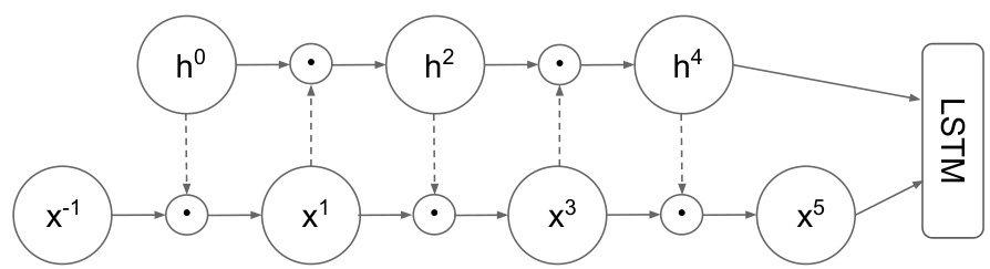
Figure 1: Mogrifier with 5 rounds of updates. The previous state $\pmb{h}^{0}=\pmb{h}_{p r e\nu}$ is transformed linearly (dashed arrows), fed through a sigmoid and gates ${\pmb x}^{-1}={\pmb x}$ in an element wise manner producing $\pmb{x}^{1}$ . Conversely, the linearly transformed $\scriptstyle{\pmb x}^{1}$ gates $\ensuremath{\boldsymbol{h}}^{0}$ and produces $\scriptstyle{h^{2}}$ . After a number of repetitions of this mutual gating cycle, the last values of $\boldsymbol{h}^{*}$ and ${\pmb x}^{*}$ sequences are fed to an LSTM cell. The prev subscript of $^{h}$ is omitted to reduce clutter.
图 1: 经过5轮更新的Mogrifier。先前状态$\pmb{h}^{0}=\pmb{h}_{p r e\nu}$经过线性变换(虚线箭头),通过sigmoid函数并与${\pmb x}^{-1}={\pmb x}$逐元素门控生成$\pmb{x}^{1}$。反之,线性变换后的$\scriptstyle{\pmb x}^{1}$对$\ensuremath{\boldsymbol{h}}^{0}$进行门控并生成$\scriptstyle{h^{2}}$。经过多轮这种相互门控循环后,最终的$\boldsymbol{h}^{*}$和${\pmb x}^{*}$序列值被输入LSTM单元。为简化图示,省略了$^{h}$的prev下标。
- with a separate transition matrix for each possible input, and the Multiplicative RNN (Sutskever et al. 2011), which factorizes the three-way tensor of stacked transition matrices. Also following this line of research are the Multiplicative Integration LSTM (Wu et al. 2016) and – closest to our model in the literature – the Multiplicative LSTM (Krause et al. 2016). The results in Section 3.4 demonstrate the utility of our approach, which consistently improves on the LSTM and establishes a new state of the art on all but the largest dataset, Enwik8, where we match similarly sized transformer models.
- 为每个可能的输入使用单独的转移矩阵,以及乘性RNN (Sutskever et al. 2011) ,后者对堆叠转移矩阵的三维张量进行分解。同样沿袭这一研究路线的还有乘性集成LSTM (Wu et al. 2016) ,以及与我们模型最为接近的文献成果——乘性LSTM (Krause et al. 2016) 。第3.4节的实验结果表明,我们的方法能持续改进LSTM性能,并在除最大数据集Enwik8外的所有基准上创造了新纪录。在Enwik8数据集上,我们的模型达到了与同等规模Transformer模型相当的水平。
2 MODEL
2 模型
To allow for ease of subsequent extension, we present the standard LSTM update (Sak et al. 2014) with input and state of size $m$ and $n$ respectively as the following function:
为了便于后续扩展,我们将标准 LSTM (Sak et al. 2014) 的更新表示为以下函数,其输入和状态大小分别为 $m$ 和 $n$:
$$
\begin{array}{r l}&{\mathrm{LSTM}\colon\mathbb{R}^{m}\times\mathbb{R}^{n}\times\mathbb{R}^{n}\to\mathbb{R}^{n}\times\mathbb{R}^{n}}\ &{\quad\mathrm{LSTM}(\pmb{x},\pmb{c}{p r e\nu},\pmb{h}_{p r e\nu})=(\pmb{c},\pmb{h}).}\end{array}
$$
$$
\begin{array}{r l}&{\mathrm{LSTM}\colon\mathbb{R}^{m}\times\mathbb{R}^{n}\times\mathbb{R}^{n}\to\mathbb{R}^{n}\times\mathbb{R}^{n}}\ &{\quad\mathrm{LSTM}(\pmb{x},\pmb{c}{p r e\nu},\pmb{h}_{p r e\nu})=(\pmb{c},\pmb{h}).}\end{array}
$$
The updated state $_c$ and the output $^{h}$ are computed as follows:
更新后的状态 $_c$ 和输出 $^{h}$ 计算如下:
$$
\begin{array}{r l}&{f=\sigma(\mathbf{W}^{f x}x+\mathbf{W}^{f h}h_{p r e v}+b^{f})}\ &{i=\sigma(\mathbf{W}^{i x}x+\mathbf{W}^{i h}h_{p r e v}+b^{i})}\ &{j=\operatorname{tanh}(\mathbf{W}^{j x}x+\mathbf{W}^{j h}h_{p r e v}+b^{j})}\ &{o=\sigma(\mathbf{W}^{o x}x+\mathbf{W}^{o h}h_{p r e v}+b^{o})}\ &{c=f\odot c_{p r e v}+i\odot j}\ &{h=o\odot\operatorname{tanh}(c),}\end{array}
$$
$$
\begin{array}{r l}&{f=\sigma(\mathbf{W}^{f x}x+\mathbf{W}^{f h}h_{p r e v}+b^{f})}\ &{i=\sigma(\mathbf{W}^{i x}x+\mathbf{W}^{i h}h_{p r e v}+b^{i})}\ &{j=\operatorname{tanh}(\mathbf{W}^{j x}x+\mathbf{W}^{j h}h_{p r e v}+b^{j})}\ &{o=\sigma(\mathbf{W}^{o x}x+\mathbf{W}^{o h}h_{p r e v}+b^{o})}\ &{c=f\odot c_{p r e v}+i\odot j}\ &{h=o\odot\operatorname{tanh}(c),}\end{array}
$$
where $\sigma$ is the logistic sigmoid function, $\odot$ is the element wise product, $\mathbf{W}^{**}$ and $b^{*}$ are weight matrices and biases.
其中$\sigma$是逻辑S型函数,$\odot$是逐元素乘积,$\mathbf{W}^{**}$和$b^{*}$是权重矩阵和偏置。
While the LSTM is typically presented as a solution to the vanishing gradients problem, its gate $i$ can also be interpreted as scaling the rows of weight matrices $\mathbf{W}^{j*}$ (ignoring the non-linearity in $j)$ . In this sense, the LSTM nudges Elman Networks towards context-dependent transitions and the extreme case of Input Switched Affine Networks. If we took another, larger step towards that extreme, we could end up with Hyper networks (Ha et al. 2016). Here, instead, we take a more cautious step, and equip the LSTM with gates that scale the columns of all its weight matrices $\mathbf{W}^{**}$ in a context-dependent manner. The scaling of the matrices $\mathbf{W}^{*x}$ (those that transform the cell input) makes the input embeddings dependent on the cell state, while the scaling of $\mathbf{W}^{*h}$ does the reverse.
虽然LSTM通常被提出作为梯度消失问题的解决方案,但其门控$i$也可以解释为对权重矩阵$\mathbf{W}^{j*}$的行进行缩放(忽略$j$中的非线性)。从这个角度看,LSTM将Elman网络推向上下文相关的转换,并接近输入切换仿射网络的极端情况。如果我们向这个极端再迈出更大一步,可能会得到超网络(Ha等人,2016)。但在这里,我们采取了更为谨慎的步骤,为LSTM配备了能够以上下文相关方式缩放所有权重矩阵$\mathbf{W}^{**}$列的门控。对矩阵$\mathbf{W}^{*x}$(那些转换单元输入的矩阵)的缩放使得输入嵌入依赖于单元状态,而对$\mathbf{W}^{*h}$的缩放则起到相反作用。
The Mogrifier1 LSTM is an LSTM where two inputs ${x}$ and $h_{p r e\nu}$ modulate one another in an alternating fashion before the usual LSTM computation takes place (see Fig. 1). That is, Mogrify $({\pmb x},{\pmb c}{p r e\nu},{\pmb h}{p r e\nu})=\mathrm{LSTM}({\pmb x}^{\uparrow},{\pmb c}{p r e\nu},{\pmb h}{p r e\nu}^{\uparrow})$ where the modulated inputs $\scriptstyle{\mathbf{\mathit{x}}}^{\uparrow}$ and $h_{p r e\nu}^{\uparrow}$ are defined as the highest indexed $\pmb{x}^{i}$ and $h_{p r e\nu}^{i}$ , respectively, from the interleaved sequences
Mogrifier1 LSTM是一种LSTM变体,在常规LSTM计算前,两个输入$x$和$h_{pre\nu}$会以交替方式相互调制(见图1)。具体而言,Mogrify$({\pmb x},{\pmb c}{pre\nu},{\pmb h}{pre\nu})=\mathrm{LSTM}({\pmb x}^{\uparrow},{\pmb c}{pre\nu},{\pmb h}{pre\nu}^{\uparrow})$,其中调制后的输入$\scriptstyle{\mathbf{\mathit{x}}}^{\uparrow}$和$h_{pre\nu}^{\uparrow}$分别定义为交错序列中最高索引的$\pmb{x}^{i}$和$h_{pre\nu}^{i}$。
$$
\begin{array}{r}{\pmb{x}^{i}=2\sigma(\mathbf{Q}^{i}\pmb{h}_{p r e\nu}^{i-1})\odot\pmb{x}^{i-2},\qquad\mathrm{foroddi\in[1....~}]}\end{array}
$$
$$
h_{p r e v}^{i}=2\sigma(\mathbf{R}^{i}x^{i-1})\odot h_{p r e v}^{i-2},\qquad\mathrm{for even i\in[1~....~}r]
$$
with ${\pmb x}^{-1}={\pmb x}$ and $h_{p r e\nu}^{0}=h_{p r e\nu}$ . The number of “rounds”, $r\in\mathbb{N}$ , is a hyper parameter; $r=0$ recovers the LSTM. Multiplication with the constant 2 ensures that randomly initialized ${\bf Q}^{i},{\bf R}^{i}$ matrices result in transformations close to identity. To reduce the number of additional model parameters, we typically factorize the ${\bf Q}^{i},{\bf R}^{i}$ matrices as products of low-rank matrices: $\mathbf{Q}^{i}=$ $\mathbf{\dot{Q}}_{\mathrm{left}}^{i}\mathbf{Q}_{\mathrm{right}}^{i}$ with $\dot{\mathbf{Q}^{i}}\in\mathbb{R}^{\dot{m}\times n}$ , $\mathbf{Q}_{\mathrm{left}}^{i}\in\mathbb{R}^{m\times k}$ , $\mathbf{Q}_{\mathrm{right}}^{i}\in\mathbb{R}^{k\times n}$ , where $k<m i n(m,n)$ is the rank.
其中 ${\pmb x}^{-1}={\pmb x}$ 且 $h_{p r e\nu}^{0}=h_{p r e\nu}$。循环轮数 $r\in\mathbb{N}$ 是一个超参数;当 $r=0$ 时即退化为LSTM。乘以常数2可确保随机初始化的 ${\bf Q}^{i},{\bf R}^{i}$ 矩阵产生的变换接近恒等变换。为减少新增模型参数量,我们通常将 ${\bf Q}^{i},{\bf R}^{i}$ 矩阵分解为低秩矩阵的乘积:$\mathbf{Q}^{i}=$ $\mathbf{\dot{Q}}_{\mathrm{left}}^{i}\mathbf{Q}_{\mathrm{right}}^{i}$,其中 $\dot{\mathbf{Q}^{i}}\in\mathbb{R}^{\dot{m}\times n}$,$\mathbf{Q}_{\mathrm{left}}^{i}\in\mathbb{R}^{m\times k}$,$\mathbf{Q}_{\mathrm{right}}^{i}\in\mathbb{R}^{k\times n}$,这里 $k<m i n(m,n)$ 表示秩。
3 EXPERIMENTS
3 实验
3.1 THE CASE FOR SMALL-SCALE
3.1 小规模 (small-scale) 的合理性
Before describing the details of the data, the experimental setup and the results, we take a short detour to motivate work on smaller-scale datasets. A recurring theme in the history of sequence models is that the problem of model design is intermingled with opt i miz ability and s cal ability. Elman Networks are notoriously difficult to optimize, a property that ultimately gave birth to the idea of the LSTM, but also to more recent models such as the Unitary Evolution RNN (Arjovsky et al. 2016) and fixes like gradient clipping (Pascanu et al. 2013). Still, it is far from clear – if we could optimize these models well – how different their biases would turn out to be. The non-se par ability of model and optimization is fairly evident in these cases.
在详细描述数据、实验设置和结果之前,我们先简要探讨小规模数据集研究的意义。序列模型发展史中反复出现的主题是:模型设计问题始终与可优化性 (optimizability) 和可扩展性 (scalability) 相互交织。Elman网络 notoriously难以优化,这一特性不仅催生了LSTM的诞生,也衍生了Unitary Evolution RNN (Arjovsky et al. 2016) 等新模型以及梯度裁剪 (gradient clipping) (Pascanu et al. 2013) 等修正方法。但即便能完美优化这些模型,其偏差表现仍存在巨大不确定性。在这些案例中,模型与优化的不可分割性 (non-separability) 表现得尤为明显。
S cal ability, on the other hand, is often optimized for indirectly. Given the limited ability of current models to generalize, we often compensate by throwing more data at the problem. To fit a larger dataset, model size must be increased. Thus the best performing models are evaluated based on their s cal ability 3. Today, scaling up still yields tangible gains on down-stream tasks, and language modelling data is abundant. However, we believe that simply scaling up will not solve the generalization problem and better models will be needed. Our hope is that by choosing small enough datasets, so that model size is no longer the limiting factor, we get a number of practical advantages:
另一方面,可扩展性(Scalability)通常被间接优化。鉴于当前模型泛化能力有限,我们常通过投入更多数据来弥补。为适配更大数据集,必须增加模型规模。因此最佳性能模型往往基于其可扩展性3进行评估。当前,扩大规模仍能在下游任务中获得显著收益,且语言建模数据充足。但我们认为单纯扩大规模无法解决泛化问题,仍需更好的模型。通过选择足够小的数据集(使模型规模不再成为限制因素),我们期望获得多项实践优势:
$\star$ Generalization ability will be more clearly reflected in evaluations even without domain adaptation. $\star$ Turnaround time in experiments will be reduced, and the freed up computational budget can be put to good use by controlling for nuisance factors. $\star$ The transient effects of changing hardware performance characteristics are somewhat lessened.
$\star$ 即使没有领域适应 (domain adaptation) ,泛化能力也能在评估中更清晰地体现。
$\star$ 实验中的周转时间将缩短,释放出的计算资源可通过控制干扰因素得到有效利用。
$\star$ 硬件性能特性变化带来的瞬时影响会有所减弱。
Thus, we develop, analyse and evaluate models primarily on small datasets. Evaluation on larger datasets is included to learn more about the models’ scaling behaviour and because of its relevance for applications, but it is to be understood that these evaluations come with much larger error bars and provide more limited guidance for further research on better models.
因此,我们主要基于小型数据集进行模型开发、分析与评估。引入大规模数据集评估旨在深入了解模型的扩展特性及其应用价值,但需注意此类评估存在更大误差范围,对优化模型的后续研究指导作用较为有限。
3.2 DATASETS
3.2 数据集
We compare models on both word and character-level language modelling datasets. The two wordlevel datasets we picked are the Penn Treebank (PTB) corpus by Marcus et al. (1993) with preprocessing from Mikolov et al. (2010) and Wikitext-2 by Merity et al. (2016), which is about twice the size of PTB with a larger vocabulary and lighter preprocessing. These datasets are definitely on the small side, but – and because of this – they are suitable for exploring different model biases. Their main shortcoming is the small vocabulary size, only in the tens of thousands, which makes them inappropriate for exploring the behaviour of the long tail. For that, open vocabulary language modelling and byte pair encoding (Sennrich et al. 2015) would be an obvious choice. Still, our primary goal here is the comparison of the LSTM and Mogrifier architectures, thus we instead opt for character-based language modelling tasks, where vocabulary size is not an issue, the long tail is not truncated, and there are no additional hyper parameters as in byte pair encoding that make fair comparison harder. The first character-based corpus is Enwik8 from the Hutter Prize dataset (Hutter 2012). Following common practice, we use the first 90 million characters for training and the remaining 10 million evenly split between validation and test. The character-level task on the
我们在词级和字符级语言建模数据集上对模型进行了比较。选取的两个词级数据集分别是Marcus等人(1993)提出的Penn Treebank(PTB)语料库(采用Mikolov等人(2010)的预处理方法)和Merity等人(2016)发布的Wikitext-2。Wikitext-2的规模约为PTB的两倍,词汇量更大且预处理更轻量。这些数据集规模确实偏小,但也正因如此适合探索不同的模型偏差。其主要缺点是词汇量过小(仅数万量级),不适合研究长尾分布行为。针对长尾分布,开放词汇语言建模和字节对编码(Sennrich等人2015)会是更合适的选择。不过本研究的主要目标是比较LSTM和Mogrifier架构,因此我们转而选择基于字符的语言建模任务——这类任务不存在词汇量限制,长尾分布不会被截断,也没有字节对编码中那些影响公平比较的额外超参数。第一个字符级语料库是Hutter Prize数据集(Hutter 2012)中的Enwik8。按照惯例,我们使用前9000万个字符进行训练,剩余1000万字符平均分配给验证集和测试集。字符级任务在...
Table 1: Word-level perplexities of near state-of-the-art models, our LSTM baseline and the Mogrifier on PTB and Wikitext-2. Models with Mixture of Softmaxes (Yang et al. 2017) are denoted with MoS, depth N with dN. MC stands for Monte-Carlo dropout evaluation. Previous state-of-the-art results in italics. Note the comfortable margin of 2.8–4.3 perplexity points the Mogrifier enjoys over the LSTM.
表 1: 当前接近最优模型的词级困惑度、我们的LSTM基线以及PTB和Wikitext-2上的Mogrifier模型。使用混合Softmax (Yang et al. 2017) 的模型标记为MoS,深度N标记为dN。MC代表蒙特卡洛dropout评估。先前最优结果以斜体显示。注意Mogrifier相比LSTM具有2.8-4.3困惑点的明显优势。
| 无Dyneval | Dyneval | ||||
|---|---|---|---|---|---|
| Val. | Test | Val. | |||
| FRAGE (d3, MoS15) (Gong et al. 2018) | 22M | 54.1 | 52.4 | 47.4 | 46.5 |
| AWD-LSTM (d3, MoS15) (Yang et al. 2017) | 22M | 56.5 | 54.4 | 48.3 | 47.7 |
| Transformer-XL (Dai et al. 2019) | 24M | 56.7 | 54.5 | ||
| LSTM (d2) | 24M | 55.8 | 54.6 | 48.9 | 48.4 |
| Mogrifier (d2) | 24M | 52.1 | 51.0 | 45.1 | 45.0 |
| LSTM (d2, MC) | 24M | 55.5 | 54.1 | 48.6 | 48.4 |
| Mogrifier (d2, MC) | 24M | 51.4 | 50.1 | 44.9 | 44.8 |
| 12 W | FRAGE (d3,MoS15) (Gong et al.2018) | 35M | 60.3 | 58.0 | 40.8 |
| AWD-LSTM (d3, MoS15) (Yang et al. 2017) | 35M | 63.9 | 61.2 | 42.4 | 40.7 |
| LSTM (d2, MoS2) | 35M | 62.6 | 60.1 | 43.2 | 41.5 |
| Mogrifier (d2,MoS2) | 35M | 58.7 | 56.6 | 40.6 | 39.0 |
| LSTM (d2, MoS2, MC) | 35M | 61.9 | 59.4 | 43.2 | 41.4 |
| Mogrifier (d2, MoS2, MC) | 35M | 57.3 | 55.1 | 40.2 | 38.6 |
Mikolov pre processed PTB corpus (Merity et al. 2018) is unique in that it has the disadvantages of closed vocabulary without the advantages of word-level modelling, but we include it for comparison to previous work. The final character-level dataset is the Multilingual Wikipedia Corpus (MWC, Kawakami et al. (2017)), from which we focus on the English and Finnish language sub datasets in the single text, large setting.
Mikolov预处理的PTB语料库(Merity等人,2018)的独特之处在于,它既具有封闭词汇的缺点,又不具备词级建模的优点,但我们仍将其纳入以与之前的工作进行比较。最终的字符级数据集是多语言维基百科语料库(MWC,Kawakami等人(2017)),我们重点关注其中单文本、大规模设置下的英语和芬兰语子数据集。
3.3 SETUP
3.3 设置
We tune hyper parameters following the experimental setup of Melis et al. (2018) using a black-box hyper parameter tuner based on batched Gaussian Process Bandits (Golovin et al. 2017). For the LSTM, the tuned hyper parameters are the same: input embedding ratio, learning rate, l2_penalty, input dropout, inter layer dropout, state dropout, output dropout. For the Mogrifier, the number of rounds $r$ and the rank $k$ of the low-rank approximation is also tuned (allowing for full rank, too). For word-level tasks, BPTT (Werbos et al. 1990) window size is set to 70 and batch size to 64. For character-level tasks, BPTT window size is set to 150 and batch size to 128 except for Enwik8 where the window size is 500. Input and output embeddings are tied for word-level tasks following Inan et al. (2016) and Press and Wolf (2016). Optimization is performed with Adam (Kingma and Ba 2014) with $\beta_{1}=0$ , a setting that resembles RMSProp without momentum. Gradients are clipped (Pascanu et al. 2013) to norm 10. We switch to averaging weights similarly to Merity et al. (2017) after a certain number of checkpoints with no improvement in validation cross-entropy or at $80%$ of the training time at the latest. We found no benefit to using two-step finetuning.
我们按照Melis等人 (2018) 的实验设置,使用基于批量高斯过程赌博机 (Golovin等人 2017) 的黑盒超参数调优器进行超参数调优。对于LSTM,调优的超参数相同:输入嵌入比例、学习率、l2惩罚项、输入dropout、层间dropout、状态dropout、输出dropout。对于Mogrifier,还调优了轮数$r$和低秩近似的秩$k$(也允许全秩)。在词级任务中,BPTT (Werbos等人 1990) 窗口大小设为70,批大小为64。在字符级任务中,BPTT窗口大小设为150,批大小为128,但Enwik8的窗口大小为500。根据Inan等人 (2016) 和Press与Wolf (2016) 的研究,词级任务的输入和输出嵌入是绑定的。优化使用Adam (Kingma和Ba 2014) 进行,其中$\beta_{1}=0$,这一设置类似于不带动量的RMSProp。梯度裁剪 (Pascanu等人 2013) 的范数阈值为10。我们采用与Merity等人 (2017) 类似的方式,在验证集交叉熵没有改善或最晚在训练时间达到$80%$时切换为权重平均。我们发现使用两步微调没有益处。
Model evaluation is performed with the standard, deterministic dropout approximation or MonteCarlo averaging (Gal and Ghahramani 2016) where explicitly noted (MC). In standard dropout evaluation, dropout is turned off while in MC dropout predictions are averaged over randomly sampled dropout masks (200 in our experiments). Optimal softmax temperature is determined on the validation set, and in the MC case dropout rates are scaled (Melis et al. 2018). Finally, we report results with and without dynamic evaluation (Krause et al. 2017). Hyper parameters for dynamic evaluation are tuned using the same method (see Appendix A for details).
模型评估采用标准确定性dropout近似或蒙特卡洛平均法 (Gal和Ghahramani 2016) (特别标注为MC时)。标准dropout评估会关闭dropout,而MC dropout预测则对随机采样的dropout掩码进行平均 (实验中采用200次)。最优softmax温度在验证集上确定,MC情况下会缩放dropout率 (Melis等人 2018)。最终,我们汇报了使用与不使用动态评估 (Krause等人 2017) 的结果。动态评估的超参数采用相同方法调优 (详见附录A)。
We make the code and the tuner output available at https://github.com/deepmind/lamb.
我们已将代码和调谐器输出发布于 https://github.com/deepmind/lamb。
3.4 RESULTS
3.4 结果
Table 1 lists our results on word-level datasets. On the PTB and Wikitext-2 datasets, the Mogrifier has lower perplexity than the LSTM by 3–4 perplexity points regardless of whether or not dynamic evaluation (Krause et al. 2017) and Monte-Carlo averaging are used. On both datasets, the state of the art is held by the AWD LSTM (Merity et al. 2017) extended with Mixture of Softmaxes (Yang et al. 2017) and FRAGE (Gong et al. 2018). The Mogrifier improves the state of the art without either of these methods on PTB, and without FRAGE on Wikitext-2.
表 1 列出了我们在词级数据集上的结果。在 PTB 和 Wikitext-2 数据集上,无论是否使用动态评估 (Krause et al. 2017) 和蒙特卡洛平均,Mogrifier 的困惑度都比 LSTM 低 3-4 个点。在这两个数据集上,当前最优结果是由结合了混合 Softmax (Yang et al. 2017) 和 FRAGE (Gong et al. 2018) 的 AWD LSTM (Merity et al. 2017) 保持的。Mogrifier 在 PTB 上无需这两种方法、在 Wikitext-2 上无需 FRAGE 就实现了对当前最优结果的超越。
Table 2: Bits per character on character-based datasets of near state-of-the-art models, our LSTM baseline and the Mogrifier. Previous state-of-the-art results in italics. Depth N is denoted with dN. MC stands for Monte-Carlo dropout evaluation. Once again the Mogrifier strictly dominates the LSTM and sets a new state of the art on all but the Enwik8 dataset where with dynamic evaluation it closes the gap to the Transformer-XL of similar size $\mathrm{\Delta}^{\prime}\dagger$ Krause et al. (2019), $\ddagger$ Ben Krause, personal communications, May 17, 2019). On most datasets, model size was set large enough for under fitting not to be an issue. This was very much not the case with Enwik8, so we grouped models of similar sizes together for ease of comparison. Unfortunately, a couple of dynamic evaluation test runs diverged (NaN) on the test set and some were just too expensive to run (Enwik8, MC).
表 2: 基于字符数据集上接近最优模型的每字符比特数、我们的LSTM基线及Mogrifier结果。先前最优结果以斜体显示。深度N用dN表示。MC代表蒙特卡洛dropout评估。Mogrifier再次全面超越LSTM,并在除Enwik8外的所有数据集上创下新纪录。在Enwik8上,通过动态评估缩小了与同规模Transformer-XL的差距 ($\mathrm{\Delta}^{\prime}\dagger$ Krause等人 (2019), $\ddagger$ Ben Krause个人交流,2019年5月17日)。多数数据集的模型尺寸足够大,不存在欠拟合问题,但Enwik8明显例外,因此我们将相近尺寸模型分组以便比较。遗憾的是,部分动态评估测试运行在测试集上发散(NaN),有些则运行成本过高(Enwik8, MC)。
| 无动态评估 | 动态评估 | |||||
|---|---|---|---|---|---|---|
| 验证集 | 测试集 | 验证集 | 测试集 | |||
| BZPE | Trellis Networks (Bai等人 2018) | 13.4M | 1.159 | |||
| AWD-LSTM (d3) (Merity等人 2017) | 13.8M | 1.175 | ||||
| LSTM (d2) | 24M | 1.163 | 1.143 | 1.116 | 1.103 | |
| Mogrifier (d2) | 24M | 1.149 | 1.131 | 1.098 | 1.088 | |
| LSTM (d2, MC) | 24M | 1.159 | 1.139 | 1.115 | 1.101 | |
| Mogrifier (d2, MC) | 24M | 1.137 | 1.120 | 1.094 | 1.083 | |
| HCLM with Cache (Kawakami等人 2017) | 8M | 1.591 | 1.538 | |||
| CMWEN | LSTM (d1) (Kawakami等人 2017) | 8M | 1.793 | 1.736 | ||
| LSTM (d2) | 24M | 1.353 | 1.338 | 1.239 | 1.225 | |
| Mogrifier (d2) | 24M | 1.319 | 1.305 | 1.202 | 1.188 | |
| LSTM (d2, MC) | 24M | 1.346 | 1.332 | 1.238 | NaN | |
| Mogrifier (d2, MC) | 24M | 1.312 | 1.298 | 1.200 | 1.187 | |
| CMWE | HCLM with Cache (Kawakami等人 2017) | 8M | 1.754 | 1.711 | ||
| LSTM (d1) (Kawakami等人 2017) | 8M | 1.943 | 1.913 | |||
| LSTM (d2) | 24M | 1.382 | 1.367 | 1.249 | 1.237 | |
| Mogrifier (d2) | 24M | 1.338 | 1.326 | 1.202 | 1.191 | |
| LSTM (d2, MC) | 24M | 1.377 | 1.361 | 1.247 | 1.234 | |
| Mogrifier (d2, MC) | 24M | 1.327 | 1.313 | 1.198 | NaN | |
| Enwik8 EN | Transformer-XL (d24) (Dai等人 2019) | 277M | 0.993 | 0.940 | ||
| Transformer-XL (d18) (Dai等人 2019) | 88M | 1.03 | ||||
| LSTM (d4) | 96M | 1.145 | 1.155 | 1.041 | 1.020 | |
| Mogrifier (d4) | 96M | 1.110 | 1.122 | 1.009 | 0.988 | |
| LSTM (d4, MC) | 96M | 1.139 | 1.147 | |||
| Mogrifier (d4, MC) | 96M | 1.104 | 1.116 | |||
| Transformer-XL (d12) (Dai等人 2019) | 41M | 1.06 | 1.01# | |||
| AWD-LSTM (d3) (Merity等人 2017) | 47M | 1.232 | ||||
| mLSTM (d1) (Krause等人 2016) | 46M | 1.24 | 1.08 | |||
| LSTM (d4) | 48M | 1.182 | 1.195 | 1.073 | 1.051 | |
| Mogrifier (d4) | 48M | 1.135 | 1.146 | 1.035 | 1.012 | |
| LSTM (d4, MC) | 48M | 1.176 | 1.188 | |||
| Mogrifier (d4, MC) | 48M | 1.130 | 1.140 |
Table 2 lists the character-level modelling results. On all datasets, our baseline LSTM results are much better than those previously reported for LSTMs, highlighting the issue of s cal ability and experimental controls. In some cases, these unexpectedly large gaps may be down to lack of hyper parameter tuning as in the case of Merity et al. (2017), or in others, to using a BPTT window size (50) that is too small for character-level modelling (Melis et al. 2017) in order to fit the model into memory. The Mogrifier further improves on these baselines by a considerable margin. Even the smallest improvement of 0.012 bpc on the highly idiosyncratic, character-based, Mikolov pre processed PTB task is equivalent to gaining about 3 perplexity points on word-level PTB. MWC, which was built for open-vocabulary language modelling, is a much better smaller-scale character-level dataset. On the English and the Finnish corpora in MWC, the Mogrifier enjoys a gap of 0.033-0.046 bpc. Finally, on the Enwik8 dataset, the gap is 0.029-0.039 bpc in favour of the Mogrifier.
表 2 列出了字符级建模结果。在所有数据集上,我们的基线 LSTM 结果远优于之前报告的 LSTM 结果,凸显了可扩展性和实验控制的问题。某些情况下,这些异常大的差距可能归因于缺乏超参数调优 (如 Merity et al. (2017)),或使用了过小的 BPTT 窗口大小 (50) 以适应内存 (Melis et al. (2017))。Mogrifier 在此基础上进一步显著提升了性能。即使在高度特殊化的字符级 Mikolov 预处理 PTB 任务上最小的 0.012 bpc 改进,也相当于在词级 PTB 上获得约 3 个困惑度点的提升。专为开放词汇语言建模设计的 MWC 是更优的小规模字符级数据集,在 MWC 的英语和芬兰语语料库中,Mogrifier 实现了 0.033-0.046 bpc 的优势。最后在 Enwik8 数据集上,Mogrifier 以 0.029-0.039 bpc 的优势领先。

Figure 2: “No-zigzag” Mogrifier for the ablation study. Gating is always based on the original inputs.
图 2: 消融研究中使用的"无锯齿"Mogrifier结构。门控机制始终基于原始输入。

Figure 3: Perplexity vs the rounds $r$ in the PTB ablation study.
图 3: PTB消融研究中困惑度 (Perplexity) 与训练轮次 $r$ 的关系。
Table 3: PTB ablation study validation perplexities with 24M parameters.
表 3: PTB消融实验验证困惑度(24M参数)。
| Mogrifier Full rank Q', Pi | 54.1 54.6 |
| Nozigzag LSTM | 55.0 |
| mLSTM | 57.5 57.8 |
Of particular note is the comparison to Transformer-XL (Dai et al. 2019), a state-of-the-art model on larger datasets such as Wikitext-103 and Enwik8. On PTB, without dynamic evaluation, the Transformer-XL is on par with our LSTM baseline which puts it about 3.5 perplexity points behind the Mogrifier. On Enwik8, also without dynamic evaluation, the Transformer-XL has a large, 0.09 bpc advantage at similar parameter budgets, but with dynamic evaluation this gap disappears. However, we did not test the Transformer-XL ourselves, so fair comparison is not possible due to differing experimental setups and the rather sparse result matrix for the Transformer-XL.
特别值得注意的是与Transformer-XL (Dai et al. 2019) 的对比,该模型在Wikitext-103和Enwik8等大型数据集上属于最先进模型。在PTB数据集上(未使用动态评估时),Transformer-XL与我们基于LSTM的基线模型表现相当,其困惑度比Mogrifier高出约3.5个点。在Enwik8数据集上(同样未使用动态评估),Transformer-XL在参数量相近的情况下具有0.09 bpc的显著优势,但引入动态评估后这一差距即消失。不过我们并未亲自测试Transformer-XL,由于实验设置差异及Transformer-XL的测试结果矩阵较为稀疏,无法进行公平比较。
4 ANALYSIS
4 分析
4.1 ABLATION STUDY
4.1 消融实验
The Mogrifier consistently outperformed the LSTM in our experiments. The optimal settings were similar across all datasets, with $r\in{5,6}$ and $k\in[40\dots90]$ (see Appendix B for a discussion of hyper parameter sensitivity). In this section, we explore the effect of these hyper parameters and show that the proposed model is not unnecessarily complicated. To save computation, we tune all models using a shortened schedule with only 145 epochs instead of 964 and a truncated BPTT window size of 35 on the word-level PTB dataset, and evaluate using the standard, deterministic dropout approximation with a tuned softmax temperature.
在我们的实验中,Mogrifier始终优于LSTM。所有数据集上的最优设置相似,其中 $r\in{5,6}$ 且 $k\in[40\dots90]$ (关于超参数敏感性的讨论详见附录B)。本节我们将探究这些超参数的影响,并证明所提模型并非不必要的复杂。为节省计算量,我们在单词级PTB数据集上采用缩短的训练周期(仅145轮而非964轮)和截断的BPTT窗口大小(35)来调优所有模型,评估时使用经调优的softmax温度进行标准确定性dropout近似。
Fig. 3 shows that the number of rounds $r$ greatly influences the results. Second, we found the low-rank factorization of $\mathbf{Q}^{i}$ and $\mathbf{R}^{i}$ to help a bit, but the full-rank variant is close behind which is what we observed on other datasets, as well. Finally, to verify that the alternating gating scheme is not overly complicated, we condition all newly introduced gates on the original inputs ${x}$ and $h{p r e\nu}$ (see Fig. 2). That is, instead of Eq. 1 and Eq. 2 the no-zigzag updates are
图 3 显示轮数 $r$ 对结果影响显著。其次,我们发现对 $\mathbf{Q}^{i}$ 和 $\mathbf{R}^{i}$ 进行低秩分解略有帮助,但全秩变体紧随其后,这与其他数据集上的观察结果一致。最后,为验证交替门控方案不过于复杂,我们将所有新增门控条件设定为原始输入 ${x}$ 和 $h_{p r e\nu}$ (见图 2)。即无锯齿更新的公式替换为式 1 和式 2。
$$
\begin{array}{r l r l}&{}&{{\boldsymbol{x}}^{i}=2\sigma({\mathbf{Q}}^{i}h_{p r e\nu})\odot{\boldsymbol{x}}^{i-2}\qquad}&&{\mathrm{ forodd i\in[1\cdot...}r],}\ &{}&{h_{p r e\nu}^{i}=2\sigma({\mathbf{R}}^{i}{\boldsymbol{x}})\odot h_{p r e\nu}^{i-2}\qquad}&&{\mathrm{for even~i\in[1\cdot...}r].}\end{array}
$$
In our experiments, the no-zigzag variant under performed the baseline Mogrifier by a small but significant margin, and was on par with the $r=2$ model in Fig. 3 suggesting that the Mogrifier’s iterative refinement scheme does more than simply widen the range of possible gating values of ${x}$ and $h_{p r e\nu}$ to $(0,2^{\lceil r/2\rceil})$ and $\left(0,2^{\lfloor r/2\rfloor}\right)$ , respectively.
在我们的实验中,无锯齿变体表现略低于基线Mogrifier模型(差距虽小但显著),与图3中 $r=2$ 的模型表现相当。这表明Mogrifier的迭代优化机制不仅简单地将 ${x}$ 和 $h_{p r e\nu}$ 的门控值范围分别扩展至 $(0,2^{\lceil r/2\rceil})$ 和 $\left(0,2^{\lfloor r/2\rfloor}\right)$。
4.2 COMPARISON TO THE MLSTM
4.2 与MLSTM的对比
The Multiplicative LSTM (Krause et al. 2016), or mLSTM for short, is closest to our model in the literature. It is defined as $\mathrm{mLSTM}({\pmb x},{\pmb c}{p r e\nu},{\pmb h}{p r e\nu})=\mathrm{LSTM}({\pmb x},{\pmb c}{p r e\nu},{\pmb h}{p r e\nu}^{m})$ , where $h_{p r e\nu}^{m}=$ $\left(\mathbf{W}^{m x}\pmb{x}\right)\odot\left(\mathbf{W}^{m h}h_{p r e\nu}\right)$ . In this formulation, the differences are readily apparent. First, the mLSTM allows for multiplicative interaction between ${x}$ and $h_{p r e\nu}$ , but it only overrides $h_{p r e\nu}$ , while in the Mogrifier the interaction is two-way, which – as the ablation study showed – is important. Second, the mLSTM can change not only the magnitude but also the sign of values in $h_{p r e\nu}$ , something with which we experimented in the Mogrifier, but could not get to work. Furthermore, in the definition of $h_{p r e\nu}^{m}$ , the unsquashed linear i ties and their element wise product make the mLSTM more sensitive to initialization and unstable during optimization.
乘法长短期记忆网络 (Multiplicative LSTM,简称mLSTM) (Krause et al. 2016) 是文献中与我们的模型最接近的变体。其定义为 $\mathrm{mLSTM}({\pmb x},{\pmb c}{p r e\nu},{\pmb h}{p r e\nu})=\mathrm{LSTM}({\pmb x},{\pmb c}{p r e\nu},{\pmb h}{p r e\nu}^{m})$ ,其中 $h_{p r e\nu}^{m}=$ $\left(\mathbf{W}^{m x}\pmb{x}\right)\odot\left(\mathbf{W}^{m h}h_{p r e\nu}\right)$ 。该架构的差异点显而易见:首先,mLSTM虽然允许 ${x}$ 与 $h_{p r e\nu}$ 之间的乘法交互,但仅会覆盖 $h_{p r e\nu}$ ,而Mogrifier实现了双向交互(消融研究表明该特性至关重要);其次,mLSTM不仅能改变 $h_{p r e\nu}$ 中数值的幅度,还能改变其符号(我们在Mogrifier中尝试过类似设计但未能实现);此外,在 $h_{p r e\nu}^{m}$ 的定义中,未压缩的线性关系及其逐元素乘积使得mLSTM对初始化更敏感,且在优化过程中稳定性较差。

Figure 4: Cross-entropy vs sequence length in the reverse copy task with i.i.d. tokens. Lower is better. The Mogrifier is better than the LSTM even in this synthetic task with no resemblance to natural language.
图 4: 在独立同分布token的反向复制任务中,交叉熵随序列长度的变化。数值越低越好。即使在这个与自然语言毫无相似性的合成任务中,Mogrifier的表现也优于LSTM。
On the Enwik8 dataset, we greatly improved on the published results of the mLSTM (Krause et al. 2016). In fact, even our LSTM baseline outperformed the mLSTM by 0.03 bpc. We also conducted experiments on PTB based on our re implementation of the mLSTM following the same methodology as the ablation study and found that the mLSTM did not improve on the LSTM (see Table 3).
在Enwik8数据集上,我们大幅改进了已发布的mLSTM (Krause等人 2016) 结果。事实上,我们的LSTM基线模型甚至以0.03 bpc的优势超越了mLSTM。基于对mLSTM的重新实现,我们采用与消融研究相同的方法在PTB上进行了实验,发现mLSTM并未超越LSTM (见表3)。
Krause et al. (2016) posit and verify the recovery hypothesis which says that having just suffered a large loss, the loss on the next time step will be smaller on average for the mLSTM than for the LSTM. This was found not to be the case for the Mogrifier. Neither did we observe a significant change in the gap between the LSTM and the Mogrifier in the tied and untied embeddings settings, which would be expected if recovery was affected by ${x}$ and $h{p r e\nu}$ being in different domains.
Krause等人(2016)提出并验证了恢复假说,该假说认为在遭受重大损失后,mLSTM在下一步的平均损失将小于LSTM。但研究发现Mogrifier并不符合这一规律。在绑定与非绑定嵌入设置中,我们也没有观察到LSTM与Mogrifier之间的差距出现显著变化——若恢复过程受$x$和$h_{pre\nu}$处于不同域的影响,这种变化本应出现。
4.3 THE REVERSE COPY TASK
4.3 反向复制任务
Our original motivation for the Mogrifier was to allow the context to amplify salient and attenuate nuisance features in the input embeddings. We conduct a simple experiment to support this point of view. Consider the reverse copy task where the network reads an input sequence of tokens and a marker token after which it has to repeat the input in reverse order. In this simple sequence-tosequence learning (Sutskever et al. 2014) setup, the reversal is intended to avoid the minimal time lag problem (Hochreiter and Schmid huber 1997), which is not our focus here.
我们设计Mogrifier的初衷是让上下文能够放大输入嵌入中的显著特征并抑制干扰特征。为验证这一观点,我们进行了一个简单实验:在逆向复制任务中,网络先读取一个由token组成的输入序列和一个标记token,随后需要按逆序重复输入内容。这个简单的序列到序列学习框架(Sutskever et al. 2014)通过逆向操作规避了最小时间滞后问题(Hochreiter and Schmidhuber 1997),不过该问题并非本文研究重点。
The experimental setup is as follows. For the training set, we generate 500 000 examples by uniformly sampling a given number of tokens from a vocabulary of size 1000. The validation and test sets are constructed similarly, and contain 10 000 examples. The model consists of an independent, unidirectional encoder and a decoder, whose total number of parameters is 10 million. The decoder is initialized from the last state of the encoder. Since over fitting is not an issue here, no dropout is necessary, and we only tune the learning rate, the l2 penalty, and the embedding size for the LSTM. For the Mogrifier, the number of rounds $r$ and the rank $k$ of the low-rank approximation are also tuned.
实验设置如下。训练集通过从包含1000个token的词表中均匀采样给定数量的token,生成50万个样本。验证集和测试集以相同方式构建,各包含1万个样本。该模型由独立的单向编码器和解码器组成,参数总量为1000万。解码器从编码器的最终状态初始化。由于此处不存在过拟合问题,无需使用dropout,我们仅需调整LSTM的学习率、L2惩罚项和嵌入维度。对于Mogrifier模型,还需调整低秩逼近的轮次$r$和秩$k$。
We compare the case where both the encoder and decoder are LSTMs to where both are Mogrifiers. Fig. 4a shows that, for sequences of length 50 and 100, both models can solve the task perfectly. At higher lengths though, the Mogrifier has a considerable advantage. Examining the best hyper parameter settings found, the embedding/hidden sizes for the LSTM and Mogrifier are 498/787 vs 41/1054 at 150 steps, and 493/790 vs 181/961 at 200 steps. Clearly, the Mogrifier was able to work with a much smaller embedding size than the LSTM, which is in line with our expectations for a model with a more flexible interaction between the input and recurrent state. We also conducted experiments with a larger model and vocabulary size, and found the effect even more pronounced (see Fig. 4b).
我们比较了编码器和解码器均为LSTM与均为Mogrifier的情况。图4a显示,对于长度为50和100的序列,两种模型都能完美解决任务。但在更长的序列上,Mogrifier具有显著优势。通过检查找到的最佳超参数设置,在150步时,LSTM和Mogrifier的嵌入/隐藏大小分别为498/787和41/1054;在200步时分别为493/790和181/961。显然,Mogrifier能够使用比LSTM小得多的嵌入大小,这与我们对输入和循环状态之间具有更灵活交互的模型的预期一致。我们还用更大的模型和词汇量进行了实验,发现效果更加明显(见图4b)。
4.4 WHAT THE MOGRIFIER IS NOT
4.4 什么是Mogrifier
The results on the reverse copy task support our hypothesis that input embeddings are enriched by the Mogrifier architecture, but that cannot be the full explanation as the results of the ablation study indicate. In the following, we consider a number of hypotheses about where the advantage of the Mogrifier lies and the experiments that provide evidence against them.
反向复制任务的结果支持了我们的假设,即输入嵌入通过Mogrifier架构得到了增强,但消融研究的结果表明这并非全部原因。接下来,我们将探讨关于Mogrifier优势所在的若干假设,以及反驳这些假设的实验证据。
5 CONCLUSIONS AND FUTURE WORK
5 结论与未来工作
We presented the Mogrifier LSTM, an extension to the LSTM, with state-of-the-art results on several language modelling tasks. Our original motivation for this work was that the context-free representation of input tokens may be a bottleneck in language models and by conditioning the input embedding on the recurrent state some benefit was indeed derived. While it may be part of the explanation, this interpretation clearly does not account for the improvements brought by conditioning the recurrent state on the input and especially the applicability to character-level datasets. Positioning our work on the Multiplicative RNN line of research offers a more compelling perspective.
我们提出了Mogrifier LSTM(一种LSTM的扩展变体),在多项语言建模任务中取得了最先进成果。本研究最初动机是:输入token的无上下文表示可能成为语言模型的瓶颈,而通过将循环状态作为输入嵌入的条件确实带来了收益。虽然这能解释部分改进,但显然无法说明通过将输入作为循环状态条件所带来的提升,特别是该方法在字符级数据集上的适用性。将我们的工作定位为乘法RNN研究路线,能提供更具说服力的研究视角。
To give more credence to this interpretation, in the analysis we highlighted a number of possible alternative explanations, and ruled them all out to varying degrees. In particular, the connection to the mLSTM is weaker than expected as the Mogrifier does not exhibit improved recovery (see Section 4.2), and on PTB the mLSTM works only as well as the LSTM. At the same time, the evidence against easier optimization is weak, and the Mogrifier establishing some kind of sharing between otherwise independent LSTM weight matrices is a distinct possibility.
为了进一步支持这一解释,我们在分析中强调了几种可能的替代解释,并在不同程度上排除了它们。特别是,与mLSTM的联系比预期更弱,因为Mogrifier并未表现出更好的恢复能力(见第4.2节),且在PTB上mLSTM的表现仅与LSTM相当。同时,反对优化难度降低的证据较弱,而Mogrifier在原本独立的LSTM权重矩阵之间建立某种共享机制是一个明显的可能性。
Finally, note that as shown by Fig. 1 and Eq. 1-2, the Mogrifier is a series of preprocessing steps composed with the LSTM function, but other architectures, such as Mogrifier GRU or Mogrifier Elman Network are possible. We also leave investigations into other forms of parameter iz ation of context-dependent transitions for future work.
最后需要注意的是,如图 1 和公式 1-2 所示,Mogrifier 是由 LSTM 函数组成的一系列预处理步骤,但也可能存在其他架构,例如 Mogrifier GRU 或 Mogrifier Elman Network。我们也将对其他形式的上下文相关转换参数化研究留待未来工作。
ACKNOWLEDGMENTS
致谢
We would like to thank Ben Krause for the Transformer-XL dynamic evaluation results, Laura Rimell, Aida Nematzadeh, Angeliki Lazaridou, Karl Moritz Hermann, Daniel Fried for helping with experiments, Chris Dyer, Sebastian Ruder and Jack Rae for their valuable feedback.
我们要感谢 Ben Krause 提供的 Transformer-XL 动态评估结果,感谢 Laura Rimell、Aida Nematzadeh、Angeliki Lazaridou、Karl Moritz Hermann 和 Daniel Fried 在实验中的帮助,以及 Chris Dyer、Sebastian Ruder 和 Jack Rae 提供的宝贵反馈。
APPENDIX A HYPER PARAMETER TUNING RANGES
附录A 超参数调优范围
In all experiments, we tuned hyper parameters using Google Vizier (Golovin et al. 2017). The tuning ranges are listed in Table 4. Obviously, mo gri fier rounds and mo gri fier rank are tuned only for the Mogrifier. If input embedding ratio $\geqslant1$ , then the input/output embedding sizes and the hidden sizes are set to equal and the linear projection from the cell output into the output embeddings space is omitted. Similarly, mogrif ier_rank $\leqslant0$ is taken to mean full rank $\mathbf{Q}^{}$ , $\mathbf{R}^{}$ without factorization. Since Enwik8 is a much larger dataset, we don’t tune input embedding ratio and specify tighter tuning ranges for dropout based on preliminary experiments (see Table 5).
在所有实验中,我们使用Google Vizier (Golovin et al. 2017)调整超参数。调参范围如表4所示。显然,mogrifier_rounds和mogrifier_rank仅针对Mogrifier进行调整。若input_embedding_ratio $\geqslant1$ ,则输入/输出嵌入尺寸与隐藏层尺寸设为相等,并省略从单元输出到输出嵌入空间的线性投影。同理,mogrifier_rank $\leqslant0$ 表示采用全秩 $\mathbf{Q}^{}$ 、 $\mathbf{R}^{}$ 而不进行因式分解。由于Enwik8是更大的数据集,我们不调整input_embedding_ratio,并根据初步实验为dropout指定更严格的调参范围(见表5)。
Dynamic evaluation hyper parameters were tuned according to Table 6. The highest possible value for max time steps, the BPTT window size, was 20 for word, and 50 for character-level tasks. The batch size for estimating the mean squared gradients over the training data was set to 1024, gradient clipping was turned off, and the l2 penalty was set to zero.
动态评估超参数根据表6进行调整。最大时间步数(即BPTT窗口大小)在单词级任务中设为20,字符级任务中设为50。用于估计训练数据上均方梯度的批量大小设置为1024,梯度裁剪关闭,且l2惩罚项设为零。
Table 4: Hyper parameter tuning ranges for all tasks except Enwik8.
表 4: 除Enwik8外所有任务的超参数调优范围
| learning_rate input_embedding_ratio 12_penalty | High 0.004 2.0 | Spacing log |
| input_dropout | 1e-3 0.9 | log |
| inter_layer_dropout | 0.0 0.95 | |
| state_dropout | 0.0 | |
| | | 0.8 |
| output_dropout | 0.0 | 0.95 |
| mogrifier_rounds (r) | 0 | 6 |
| mogrifier_rank (k) | -20 | 100 |
Table 5: Hyper parameter tuning ranges for Enwik8.
表 5: Enwik8的超参数调优范围
| learning_rate | High 0.004 | Spacing log |
| 12_penalty input_dropout | 1e-3 0.2 | log |
| | | |
| inter_layer_dropout | 0.2 | |
| state_dropout | 0.25 | |
| output_dropout | 0.0 | 0.25 |
| mogrifier_rounds (r) | 0 | 6 |
| mogrifier_rank (k) | -20 | 100 |
Table 6: Hyper parameter tuning ranges for dynamic evaluation.
表 6: 动态评估的超参数调优范围
| max_time_steps | Low 1 | High 20/50 | Spacing |
|---|---|---|---|
| dyneval_learning_rate | 1e-6 | 1e-3 | log |
| dyneval_decay_rate | 1e-6 | 1e-2 | log |
| dyneval_epsilon | 1e-8 | 1e-2 | log |
APPENDIX B HYPER PARAMETER SENSITIVITY
附录 B 超参数敏感性
The parallel coordinate plots in Fig. 5 and 6, give a rough idea about hyper parameter sensitivity. The red lines correspond to hyper parameter combinations closest to the best solution found. To find the closest combinations, we restricted the range for each hyper parameter separately to about $15%$ of its entire tuning range.
图 5 和图 6 中的平行坐标图大致展示了超参数敏感性。红线对应最接近已找到最优解的超参数组合。为找出最接近的组合,我们分别将每个超参数的调整范围限制在其整体调参范围的约 15% 内。
For both the LSTM and the Mogrifier, the results are at most 1.2 perplexity points off the best result, so our results are somewhat insensitive to jitter in the hyper parameters. Still, in this setup, grid search would require orders of magnitude more trials to find comparable solutions.
对于 LSTM 和 Mogrifier 而言,结果与最佳值最多相差 1.2 个困惑度点,因此我们的结果对超参数抖动相对不敏感。不过在此设置下,网格搜索需要多几个数量级的试验才能找到可比解。
On the other hand, the tuner does take advantage of the stochastic it y of training, and repeated runs with the same parameters may be give slightly worse results. To gauge the extent of this effect, on PTB we estimated the standard deviation in reruns of the LSTM with the best hyper parameters to be about 0.2 perplexity points, but the mean was about 0.7 perplexity points off the result produced with the weights saved in best tuning run.
另一方面,调谐器确实利用了训练过程中的随机性,使用相同参数重复运行可能会产生稍差的结果。为了评估这种影响的程度,在PTB数据集上我们估计,使用最佳超参数重复运行LSTM时,困惑度的标准差约为0.2个点,但平均值与最佳调谐运行保存的权重所产生的结果相差约0.7个困惑度点。

Figure 5: Average per-word validation cross-entropies for hyper parameter combinations in the neighbourhood of the best solution for a 2-layer LSTM with 24M weights on the Penn Treebank dataset.
图 5: 在Penn Treebank数据集上,对于具有2400万权重的2层LSTM,最佳解附近超参数组合的每词平均验证交叉熵。

Figure 6: Average per-word validation cross-entropies for hyper parameter combinations in the neighbourhood of the best solution for a 2-layer Mogrifier LSTM with 24M weights on the Penn Treebank dataset. feature mask rank and feature mask rounds are aliases for mo gri fier rank and mo gri fier rounds
图 6: 在Penn Treebank数据集上,权重为24M的2层Mogrifier LSTM最佳解附近超参数组合的每词平均验证交叉熵。feature mask rank和feature mask rounds分别是mogrifier rank和mogrifier rounds的别名