Combining inherent knowledge of vision-language models with unsupervised domain adaptation through strong-weak guidance
结合视觉语言模型的固有知识与强弱引导的无监督领域自适应
Abstract
摘要
Unsupervised domain adaptation (UDA) tries to overcome the tedious work of labeling data by leveraging a labeled source dataset and transferring its knowledge to a similar but different target dataset. Meanwhile, current vision-language models exhibit remarkable zero-shot prediction capabilities. In this work, we combine knowledge gained through UDA with the inherent knowledge of visionlanguage models. We introduce a strong-weak guidance learning scheme that employs zero-shot predictions to help align the source and target dataset. For the strong guidance, we expand the source dataset with the most confident samples of the target dataset. Additionally, we employ a knowledge distillation loss as weak guidance. The strong guidance uses hard labels but is only applied to the most confident predictions from the target dataset. Conversely, the weak guidance is employed to the whole dataset but uses soft labels. The weak guidance is implemented as a knowledge distillation loss with (adjusted) zero-shot predictions. We show that our method complements and benefits from prompt adaptation techniques for vision-language models. We conduct experiments and ablation studies on three benchmarks (OfficeHome, VisDA, and DomainNet), outperforming state-of-the-art methods. Our ablation studies further demonstrate the contributions of different components of our algorithm.
无监督域适应 (UDA) 试图通过利用带标注的源数据集并将其知识迁移到相似但不同的目标数据集,从而克服数据标注的繁琐工作。与此同时,当前的视觉语言模型展现出卓越的零样本预测能力。在这项工作中,我们将通过 UDA 获得的知识与视觉语言模型的固有知识相结合。我们提出了一种强弱引导学习方案,利用零样本预测来帮助对齐源数据集和目标数据集。对于强引导,我们通过目标数据集中置信度最高的样本来扩展源数据集。此外,我们还采用知识蒸馏损失作为弱引导。强引导使用硬标签,但仅应用于目标数据集中最置信的预测。相反,弱引导应用于整个数据集,但使用软标签。弱引导通过 (调整后的) 零样本预测实现为知识蒸馏损失。我们证明了我们的方法补充并受益于视觉语言模型的提示适应技术。我们在三个基准数据集 (OfficeHome、VisDA 和 DomainNet) 上进行了实验和消融研究,性能优于最先进的方法。我们的消融研究进一步展示了算法中不同组件的贡献。
1. Introduction
1. 引言
Deep neural networks have significantly advanced the field of computer vision. However, training these networks requires a large amount of labeled data. Unsupervised domain adaptation (UDA) offers a solution by transferring knowledge from a labeled similar but distinct source dataset to an unlabeled target dataset, reducing the need for extensive labeling.
深度神经网络极大地推动了计算机视觉领域的发展。然而,训练这些网络需要大量标注数据。无监督域适应 (UDA) 通过将知识从已标注的相似但不同的源数据集迁移到未标注的目标数据集,减少了对大量标注的需求。
On the other hand, vision-language models exhibit remarkable zero-shot prediction accuracy, even without any task-specific training data. For instance, on the DomainNet dataset, current vision-language models’ zero-shot predictions outperform state-of-the-art domain adaptation without the need for a source dataset. This raises the question of the importance of domain adaption method give the rapid emergence of larger foundation models.
另一方面,视觉语言模型 (vision-language models) 展现出惊人的零样本预测精度,即使没有任何任务特定的训练数据。例如,在 DomainNet 数据集上,当前视觉语言模型的零样本预测效果优于最先进的领域自适应方法,且无需源数据集。这引发了一个问题:随着更大型基础模型的快速涌现,领域自适应方法的重要性是否依然存在。
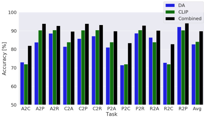
Figure 1. Accuracy on the OfficeHome dataset for unsupervised domain adaptation (blue), CLIP zero-shot predictions (green), and our combined version (black) integrating zero-shot predictions into UDA. In this work, we present a way to combine the knowledge from vision-language models with knowledge transferred via UDA from a source domain. It can be seen that the performance significantly improves.
图 1: OfficeHome数据集上无监督域适应(blue)、CLIP零样本预测(green)及我们融合零样本预测与UDA的方案(black)的准确率对比。本研究提出了一种将视觉语言模型知识与源域UDA迁移知识相结合的方法,可见性能显著提升。
In this work, we argue that rather than seeing these two methods as competing, combining the strengths of both of them achieves even better results. We combine the inherent knowledge of the vision-language models with the knowledge transferred from a source dataset through domain adaptation.
在本研究中,我们认为将这两种方法的优势相结合能取得更优效果,而非视它们为竞争关系。我们融合了视觉语言模型(Vision-Language Model)的固有知识与通过领域适应(Domain Adaptation)从源数据集迁移的知识。
To preserve the inherent knowledge of the visionlanguage model we employ a strong-weak guidance. The strong guidance is applied only for the most confident samples using the hard predictions (i.e. pseudo-label) in form of a source dataset expansion. Conversely, the weak guidance employs soft predictions and is applied to all samples in form of a knowledge distillation loss. We show that adjusting the output probabilities by accentuating the winning probabilities enhances the effectiveness of knowledge distillation.
为保留视觉语言模型的固有知识,我们采用强弱引导策略。强引导仅对置信度最高的样本应用,通过源数据集扩展形式的硬预测(即伪标签)实现。相反,弱引导采用软预测形式,以知识蒸馏损失作用于所有样本。研究表明,通过强化获胜概率来调整输出概率,能有效提升知识蒸馏的效果。
By combining our strong-weak guidance with a conventional unsupervised domain adaptation method we can significantly increase the performance as can be seen in Fig. 1. This highlights the potential of combining inherent knowledge of vision-language models with knowledge transferred from a source domain.
通过将我们的强弱引导与传统的无监督域适应方法相结合,可以显著提升性能,如图1所示。这凸显了将视觉语言模型的固有知识与从源域迁移的知识相结合的潜力。
While much research on domain adaptation with CLIP models has focused on adapting the text prompt, our method focuses on adapting the visual encoder, while maintaining its inherent knowledge. We show that these two approaches are complementary, and show that our method benefits from combining it with the prompt adaptation method DAPL [7].
虽然关于CLIP模型领域适应的研究多集中于调整文本提示(prompt),但我们的方法着重于调整视觉编码器(visual encoder),同时保留其固有知识。研究表明这两种方法具有互补性,我们的方法结合提示适应技术DAPL[7]能获得更优效果。
Our main contributions are:
我们的主要贡献包括:
2. Related works
2. 相关工作
2.1. Unsupervised domain adaptation
2.1. 无监督域适应
The goal of unsupervised domain adaptation is to overcome the domain shift between the source and the target dataset. Surveys for this task can be found in [40], [37]. One approach is to align the feature space distributions between the two datasets. Domain-adversarial neural network (DANN) [5] introduces an adversarial approach to achieve this. A domain classifier is trained to distinguish the feature space of source and target samples. The work introduced a gradient reversal layer. This layer inverts the gradients and thereby inverts the training objective, meaning that the backbone is trained to generate features that are indist ingui sh able for the domain classifier, generating so-called domain invariant features. BIWAA [29] introduces a feature re-weighting approach based on their contribution to the classifier. CDAN [17] extended DANN by multi linear conditioning the domain classifier with the classifier predictions. Moving semantic transfer network [31] introduced a moving semantic loss.
无监督域适应的目标是克服源数据集与目标数据集之间的域偏移问题。相关综述可参考[40]、[37]。其中一种方法是对齐两个数据集的特征空间分布。域对抗神经网络(DANN)[5]提出通过对抗方式实现这一目标:训练一个域分类器来区分源样本与目标样本的特征空间,并引入梯度反转层——该层通过反转梯度来逆转训练目标,使得主干网络生成域分类器无法区分的特征(即所谓域不变特征)。BIWAA[29]提出基于特征对分类器贡献度的重加权方法。CDAN[17]通过用分类器预测结果对域分类器进行多线性条件化扩展了DANN。移动语义传输网络[31]则引入了移动语义损失。
Another approach aims for the minimization of jointerror [36]. Others approaches employ information maximization or entropy minimization to generate more accurate target predictions. SHOT [16] exploits both information maximization and self-supervised pseudo-labeling to increase the performance of the target domain. SENTRY [23] uses prediction consistency among different augmentations of an image to either minimize its entropy or maximize it in case of inconsistent predictions.
另一种方法旨在最小化联合误差[36]。其他方法则采用信息最大化或熵最小化来生成更准确的目标预测。SHOT[16]结合了信息最大化和自监督伪标签技术,以提升目标域的性能。SENTRY[23]利用图像不同增强版本间的预测一致性,对预测一致的样本最小化其熵,而对不一致的样本则最大化其熵。
Following the rise of vision transformers approaches specially tailored for these backbones have gained popularity. TVT [33] introduced a Transfer ability Adaption Module that employs a patch-level domain disc rim in at or to measure the transfer ability of patch tokens, and injects learned transfer ability into the multi-head self- attention block of a transformer. CDTrans [32] introduced a triple-branch transformer framework with cross-attention between source and target domains. PMTrans [39] introduced PatchMix which builds an intermediate domain by mixing patches of source and target images. The mixing process uses a learnable Beta distribution and attention-based scoring function to assign label weights to each patch.
随着视觉Transformer的兴起,专门为这些骨干网络定制的方法日益流行。TVT [33] 提出了一个传输能力适配模块,该模块采用补丁级领域判别器来测量补丁Token的传输能力,并将学习到的传输能力注入Transformer的多头自注意力块中。CDTrans [32] 引入了一个三分支Transformer框架,具有源域和目标域之间的交叉注意力。PMTrans [39] 提出了PatchMix,通过混合源图像和目标图像的补丁来构建中间域。混合过程使用可学习的Beta分布和基于注意力的评分函数为每个补丁分配标签权重。
In our work, we employ CDAN [17] as our domain adaptation loss. While the performance is neither stateof-the-art for CNN-based nor transformer-based networks, it achieves reasonable performance for both architectures. [11] has shown that many algorithms developed for CNN backbones under perform for transformer-based backbones. On the other hand, most transformer-based algorithms explicitly make use of the network structure and cannot be employed for CNN-backbones.
在我们的工作中,我们采用CDAN [17]作为域适应损失函数。虽然该性能对于基于CNN或基于Transformer的网络都不是最先进的,但它在这两种架构上都实现了合理的性能。[11]表明,许多为CNN骨干网络开发的算法在基于Transformer的骨干网络上表现不佳。另一方面,大多数基于Transformer的算法明确利用了网络结构,无法用于CNN骨干网络。
2.2. Vision-language models
2.2. 视觉语言模型
CLIP [24] introduced a contrastive learning strategy between text and image pairs. It employs a text encoder and a visual encoder. Feature representations of positive pairs are pushed together, while unrelated or negative pairs are pushed apart. The usage of visual and language encoders enables zero-shot prediction. The class labels are encoded via the language encoder and serve as classifier. Usually, the class labels are combined with a pretext or ensemble of pretexts such as $\mathbf{\mu}_{\mathrm{\tinyR~}}$ photo of a ${{\mathrm{object}}}$ .’ to enhance the performance, where ${{\mathrm{object}}}$ is replaced with the respective classes. While CLIP collected the training dataset by constructing an allowlist of high-frequency visual concepts from Wikipedia, ALIGN [9] does not employ this step, but makes up for it by using a much larger, though noisier, dataset. BASIC [22] further increased the zero-shot prediction capabilities by further increasing data size, model size, and batch size. LiT [35] employs a pre-trained image encoder as visual backbone and aligns a text encoder to it. The vision encoder is frozen during the alignment. DFN [4] investigates data filtering networks to pool high-quality data from noisy curated web data.
CLIP [24] 提出了一种文本与图像对的对比学习策略。该方法采用文本编码器和视觉编码器,将正样本对的特征表示拉近,同时将无关或负样本对的特征推远。通过视觉与语言编码器的结合,实现了零样本预测能力。类别标签经由语言编码器编码后充当分类器,通常这些标签会与提示模板(如 $\mathbf{\mu}_{\mathrm{\tinyR~}}$ photo of a ${{\mathrm{object}}}$)或其组合相结合以提升性能,其中 ${{\mathrm{object}}}$ 会被替换为具体类别名称。CLIP通过从维基百科构建高频视觉概念白名单来收集训练数据,而ALIGN [9] 省去了这一步骤,转而使用规模更大但噪声更多的数据集进行补偿。BASIC [22] 通过进一步扩大数据规模、模型尺寸和批处理量,显著提升了零样本预测能力。LiT [35] 采用预训练图像编码器作为视觉骨干网络,并将文本编码器与之对齐,在对齐过程中保持视觉编码器参数冻结。DFN [4] 则研究了从带噪声的网络数据中筛选高质量数据的数据过滤网络。
In our work, we employ the CLIP pre-trained models due to their popularity. We employ the seven ImageNet templates subset published on the CLIP Git Hub.
在我们的工作中,由于CLIP预训练模型的广泛使用,我们采用了该模型。我们使用了CLIP GitHub上发布的七个ImageNet模板子集。
2.3. Domain adaptation for vision-language models
2.3. 视觉语言模型 (Vision-Language Models) 的领域自适应
Surprisingly there has not been much research on combining domain adaptation to vision-language models.
令人惊讶的是,关于将领域适应 (domain adaptation) 结合到视觉语言模型 (vision-language models) 中的研究并不多。
Few approaches make use of prompt learning [38]. This approach trains the prompt’s context words for the text encoder with learnable vectors while the encoder weights are frozen. DAPL [7] employs a prompt learning approach to learn domain-agnostic context variables and domainspecific context variables for unsupervised domain adaptation. This approach freezes the text and vision encoder during training. AD-CLIP [26] introduces a prompt learning scheme that entirely leverages the visual encoder of CLIP and introduces a small set of learnable projector networks. PADCLIP [12] aims for a debiasing zero-shot predictions and employs a self-training paradigm, we employ adjusted prediction scores instead of hard pseudo-labels and use an adversarial approach to overcome the domain gap. EUDA [13] employs prompt task-dependant tuning and a visual feature refinement module in combination with pseudo-labeling from semi-supervised class if i ers. MPA [3] takes a similar approach of prompt learning for multi-source unsupervised domain adaptation. In a first step, individual prompts are learned to minimize the domain gap through a contrastive loss. Then, MPA employs an auto-encoding process and aligns the learned prompts by maximizing the agreement of all the reconstructed prompts. DALLV [34] employs large language-vision models for the task of source-free video domain adaptation. They distill the world prior and complementary source model information into a student network tailored for the target. This approach also freezes the vision encoder and only learns an adapter on top of the vision encoder.
少数方法利用了提示学习[38]。该方法通过可学习向量训练文本编码器的提示上下文词,同时冻结编码器权重。DAPL[7]采用提示学习方法,针对无监督域适应任务学习领域无关上下文变量和领域特定上下文变量,训练过程中冻结文本和视觉编码器。AD-CLIP[26]提出完全利用CLIP视觉编码器的提示学习方案,并引入少量可学习的投影网络。PADCLIP[12]致力于消除零样本预测偏差,采用自训练范式——使用调整后的预测分数替代硬伪标签,并运用对抗方法克服领域差距。EUDA[13]结合半监督分类器的伪标签技术,采用任务依赖型提示调优和视觉特征精炼模块。MPA[3]对多源无监督域适应采用类似的提示学习方法:首先通过对比损失学习独立提示以最小化领域差距,随后利用自编码过程,通过最大化所有重构提示的一致性进行对齐。DALLV[34]运用大语言视觉模型完成无源视频域适应任务,将世界先验和互补源模型信息蒸馏到针对目标域定制的学生网络中,该方法同样冻结视觉编码器,仅学习视觉编码器顶部的适配器。
Unlike most of the above methods, we do not freeze the vision encoder during the training. While most of the mentioned methods focus on adapting the text prompts, we focus on adapting the visual extractor while retaining the inherent knowledge through our strong-weak guidance. We also show our method is complementary to and benefits from prompt learning methods.
与上述大多数方法不同,我们在训练期间不会冻结视觉编码器。虽然提到的方法主要侧重于调整文本提示,但我们通过强弱引导机制在保留固有知识的同时,重点优化视觉特征提取器。我们还证明该方法与提示学习方法具有互补性,并能从中受益。
3. Methodology
3. 方法论
In unsupervised domain adaptation, the goal is to transfer knowledge from a source dataset $\mathcal{D}{s}$ consisting of $n_{s}$ labeled images $\mathcal{D}{s}=(x_{i,s},y_{i,s}){i=1}^{n_{s}}$ to an unlabeled target dataset $D_{t}$ containing $n_{t}$ unlabeled data $\mathcal{D}{t}=\left(x_{i,t}\right){i=1}^{n_{t}}$ . In this work we focus on combining the inherent knowledge of vision-language models with the knowledge gained from the knowledge transfer of the source domain, meaning we further have access to the zero-shot predictions $y_{o}$ for each sample.
在无监督域适应中,目标是将知识从包含$n_{s}$个标注图像$\mathcal{D}{s}=(x_{i,s},y_{i,s}){i=1}^{n_{s}}$的源数据集$\mathcal{D}{s}$迁移到包含$n_{t}$个无标注数据$\mathcal{D}{t}=\left(x_{i,t}\right){i=1}^{n_{t}}$的无标注目标数据集$D_{t}$。本工作重点在于结合视觉语言模型(Vision-Language Model)的固有知识与源域知识迁移所获知识,这意味着我们还能获取每个样本的零样本(Zero-shot)预测结果$y_{o}$。
For the knowledge transfer from the source to the target domain, we employ the widely established adversarial domain adaptation method CDAN [17] as it was shown to be effective for both convolutional- and transformer-based network architectures [11].
为了将知识从源领域迁移到目标领域,我们采用了广泛使用的对抗性领域自适应方法CDAN [17],该方法已被证明对基于卷积和Transformer的网络架构均有效[11]。
To preserve the inherent knowledge of the visionlanguage model we employ a strong-weak guidance scheme. For the strong guidance, a hard pseudo-label is employed, but only for the most confident samples. We employ a source domain expansion inspired by GSDE [30] that copies the most confident target samples into the source domain with their predicted pseudo-label.
为保留视觉语言模型的固有知识,我们采用了强弱引导策略。强引导采用硬伪标签,但仅针对置信度最高的样本。受GSDE [30] 启发,我们实施了源域扩展策略:将置信度最高的目标样本及其预测伪标签复制到源域中。
For the weak guidance, we employ a knowledge distillation loss [8] using the zero-shot predictions. However, since the zero-shot predictions exhibit a relatively wide spread of probabilities among the classes, we first accentuate the winning probabilities. The process flow of our algorithm can be seen in Fig. 2.
对于弱监督部分,我们采用知识蒸馏损失 [8] 并利用零样本预测结果。但由于零样本预测在各类别上的概率分布较为分散,我们首先会强化优势类别的概率值。算法流程如图 2 所示。
We use the three losses:
我们采用以下三种损失函数:
$$
{\cal L}={\cal L}{C E}+{\cal L}{K D}+{\cal L}_{A D}
$$
$$
{\cal L}={\cal L}{C E}+{\cal L}{K D}+{\cal L}_{A D}
$$
where $L_{C E}$ is the classification loss for the source data, $L_{K D}$ is the knowledge distillation loss, and $L_{A D}$ is the adversarial adaptation loss. $L_{K D}$ and $L_{A D}$ are calculated for both source and target data. We further employ a strongly augmented version of source and target data, which are handled in the same way as the weakly augmented versions.
其中 $L_{C E}$ 是源数据的分类损失,$L_{K D}$ 是知识蒸馏损失,$L_{A D}$ 是对抗适应损失。$L_{K D}$ 和 $L_{A D}$ 均针对源数据和目标数据计算。我们进一步采用源数据和目标数据的强增强版本,其处理方式与弱增强版本相同。
We also show that our method is complementary to prompt learning methods by combining it with Domain Adaptation via Prompt Learning (DAPL) [7].
我们还展示了该方法与基于提示学习的领域自适应(Domain Adaptation via Prompt Learning, DAPL) [7] 结合使用时具有互补性。
3.1. Strong guidance - Source Domain Expansion:
3.1. 强引导 - 源域扩展:
For the strong guidance, we employ a source domain expansion strategy. The highest scoring zero-shot predictions are copied and appended to the source dataset with their respective pseudo-labels as pseudo-source data. We employ this source domain expansion strategy since it was shown to be more effective than simply adding a CE-loss for the respective target samples (as was shown in [30]). During training no distinction between source data and pseudosource data is made.
对于强引导,我们采用源域扩展策略。将零样本预测中得分最高的样本复制并附加到源数据集中,其对应的伪标签作为伪源数据。我们采用这种源域扩展策略,因为研究表明它比单纯为目标样本添加交叉熵损失更有效 [30]。在训练过程中,不对源数据和伪源数据进行区分。
The paper that inspired the strategy for our strong guidance employed the source domain expansion in an iterative procedure. The network was trained for several runs, each time with an increasing amount of pseudo-source data.
启发我们采用强引导策略的论文在迭代过程中运用了源域扩展方法。该网络经过多次训练,每次都会增加伪源数据的数量。
In this work, we experiment with 2 different versions. The first version trains the network a single time. The second version employs an iterative training scheme training for 2 runs. In the first run, the source domain expansion is done regarding the zero-shot predictions, and in the second run it is done regarding a mixture of zero-shot predictions and predictions generated from the previous run:
在本工作中,我们实验了两种不同版本。第一个版本对网络进行单次训练。第二个版本采用迭代训练方案,进行两次训练:第一次运行时,源域扩展基于零样本预测完成;第二次运行时,则基于零样本预测与前次运行生成预测的混合结果进行扩展:
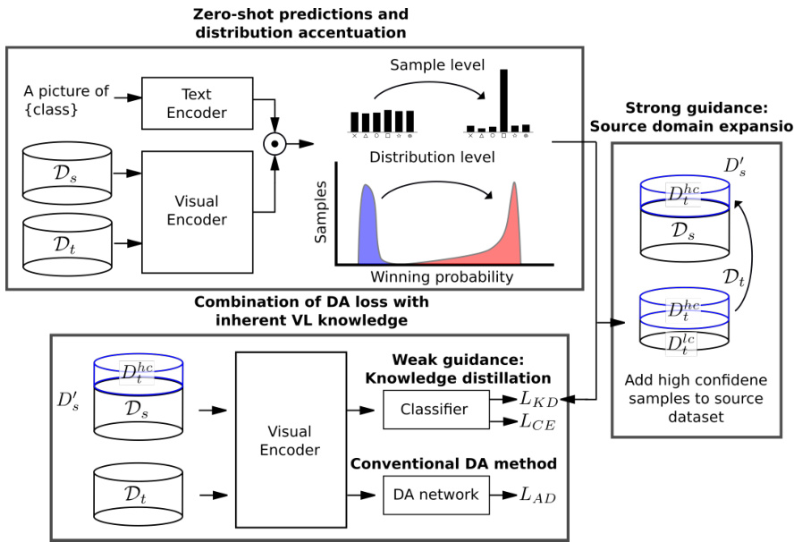
Figure 2. Process flow of our algorithm. In a first step, the zero-shot predictions of source $\mathcal{D}{s}$ and target $\mathcal{D}{t}$ dataset are estimated. We shift the zero-shot predictions distribution through a temperature parameter in the softmax to accentuate the winning probability. Based on the zero-shot predictions, we extend the source dataset with high confident target samples. These samples are treated as source data, with their respective pseudo-labels and represent the strong guidance of our method. The network is then trained using a classification loss $L_{C E}$ for the (expanded) source data, a knowledge distillation loss $L_{K D}$ employing the shifted zero-shot predictions $\tilde{y}{o}$ , and an adversarial adaptation loss $L_{D A}$ . The knowledge distillation loss represents the weak guidance of the method, as it is employed for all samples and uses the soft zero-shot predictions.
图 2: 本算法流程示意图。第一步先估计源数据集 $\mathcal{D}{s}$ 和目标数据集 $\mathcal{D}{t}$ 的零样本预测结果,通过softmax中的温度参数调整零样本预测分布以强化获胜概率。基于零样本预测,我们使用高置信度目标样本扩展源数据集,这些样本被视为带有伪标签的源数据,体现了本方法的强指导性。随后网络训练采用三项损失函数:(扩展后)源数据的分类损失 $L_{C E}$、基于调整后零样本预测 $\tilde{y}{o}$ 的知识蒸馏损失 $L_{K D}$,以及对抗适应损失 $L_{D A}$。其中知识蒸馏损失作为弱指导项,作用于所有样本并使用软化后的零样本预测结果。
$$
s(\hat{y})=p(y_{n-1})+\frac{1}{2}p(\tilde{y}_{o})
$$
$$
s(\hat{y})=p(y_{n-1})+\frac{1}{2}p(\tilde{y}_{o})
$$
where $s(\hat{y})$ depicts the scores of the samples for being chosen as pseudo-source samples, $p(y_{n-1})$ depicts the predictions of the previous run, and $p(\tilde{y}_{o})$ depicts the zero-shot predictions.
其中 $s(\hat{y})$ 表示样本被选为伪源样本的分数, $p(y_{n-1})$ 表示前一轮运行的预测结果, $p(\tilde{y}_{o})$ 表示零样本预测结果。
While the first version trains for a single run, and therefore no additional computational time is required, the second version trains for two runs, which require double the training time.
第一版训练只需单次运行,因此无需额外计算时间;而第二版训练需进行两次运行,所需训练时间翻倍。
3.2. Weak guidance - Knowledge distillation loss
3.2. 弱引导 - 知识蒸馏损失
For the weak guidance, we employ a knowledge distillation loss [8] using the zero-shot predictions. However, since the predictions are rather evenly spread among all classes, we accentuate the winning probabilities before employing them in the KD-loss (see Fig. 2). This is done through a temperature parameter $T$ in the softmax function. In a normal KD setting, the teacher’s winning prediction score usually tends to approach a one-hot vector. The goal is to mimic this setting while maintaining the relative prediction probabilities. To accomplish that we estimate the temperature parameter $T$ so that the mean winning probability over all source and target data equals to $\tau$ . We employ a value of $\tau=0.9$ in our experiments. In the estimation, we equally factor the source and target domain to further maintain the relative prediction confidence between the two domains.
对于弱监督,我们采用知识蒸馏损失[8]利用零样本预测。但由于预测结果在各类别间分布较为均匀,在应用于KD损失前会对获胜概率进行强化处理(见图2)。这一过程通过在softmax函数中引入温度参数$T$实现。在常规KD设置中,教师的获胜预测分数通常趋近于独热向量。我们的目标是在保持相对预测概率的同时模拟这种特性。为此,我们通过使所有源域和目标数据的平均获胜概率等于$\tau$来估算温度参数$T$,实验中采用$\tau=0.9$。估算时对源域和目标域进行等权处理,以进一步保持两域间的相对预测置信度。
$$
\frac{1}{2n_{s}}\sum_{n_{s}}\operatorname*{max}(\sigma(y_{o,i,s}/T))+\frac{1}{2n_{t}}\sum_{n_{t}}\operatorname*{max}(\sigma(y_{o,i,t}/T))=\tau
$$
$$
\frac{1}{2n_{s}}\sum_{n_{s}}\operatorname*{max}(\sigma(y_{o,i,s}/T))+\frac{1}{2n_{t}}\sum_{n_{t}}\operatorname*{max}(\sigma(y_{o,i,t}/T))=\tau
$$
$y_{o,i,s}$ depicts logits of the $i$ -th sample of the source data the $\sigma$ depicts the softmax-function. We then employ the adjusted zero-shot predictions for the knowledge distillation loss:
$y_{o,i,s}$ 表示源数据第 $i$ 个样本的对数几率,$\sigma$ 表示 softmax 函数。随后我们采用调整后的零样本预测来计算知识蒸馏损失:
$$
{\cal L}{K D}=D_{K L}(\tilde{y}_{o}||y)
$$
$$
{\cal L}{K D}=D_{K L}(\tilde{y}_{o}||y)
$$
where $D_{K L}$ is the Kullback-Leibler divergence loss, and $y$ is the output of the classifier of our network.
其中 $D_{K L}$ 是Kullback-Leibler散度损失,$y$ 是我们网络分类器的输出。
3.3. Adversarial loss
3.3. 对抗损失 (Adversarial loss)
We employ conditional adversarial domain adaptation loss CDAN:
我们采用条件对抗域适应损失 CDAN:
$$
L_{A D}=L_{B C E}(G_{d}((f_{i}\otimes p_{i}),d_{i}))
$$
$$
L_{A D}=L_{B C E}(G_{d}((f_{i}\otimes p_{i}),d_{i}))
$$
where $G_{d}$ is the domain classification network. $f_{i}$ are the features of sample $i$ , $p_{i}$ the class probabilities and $d_{i}$ the domain label. CDAN employs a gradient reversal layer to inverse the training objective. This means that while the domain classifier is trained to distinguish the domain (source or target) of the respective sample, the objective of the feature extractor is to extract features that are indistinguishable for the domain classifier, thereby generating domain invariant features.
其中 $G_{d}$ 是域分类网络,$f_{i}$ 表示样本 $i$ 的特征,$p_{i}$ 为类别概率,$d_{i}$ 为域标签。CDAN采用梯度反转层来反转训练目标:当域分类器被训练用于区分样本所属域(源域或目标域)时,特征提取器的目标则是生成域分类器无法区分的特征,从而产生域不变特征。
Table 1. Accuracy results on Office-Home dataset. The best results are displayed in bold and the runner-up results are underlined. Methods using a ResNet-50 backbone are on top, and methods using a transformer-based backbone are on the bottom. CLIP indicates zero-shot results of CLIP, and methods based on it are listed below it. Our methods are on the bottom, DAPL marks the combination with the prompt learning method. V1 stands for version 1 and V2 for version 2 respectively.
表 1: Office-Home数据集上的准确率结果。最佳结果以粗体显示,次优结果加下划线标注。使用ResNet-50主干网络的方法位于表格上部,基于Transformer主干网络的方法位于下部。CLIP标注了其零样本结果,基于它的方法列在其下方。我们的方法位于底部,DAPL表示与提示学习方法结合的版本。V1和V2分别代表版本1和版本2。
| 方法 - RN50 | A→C | A→P | A→R | C→A | C→P | C→R | P→A | P→C | P→R | R→A | R→C | R→P | 平均 |
|---|---|---|---|---|---|---|---|---|---|---|---|---|---|
| CDAN [17] | 50.7 | 70.6 | 76.0 | 57.6 | 70.0 | 70.0 | 57.4 | 50.9 | 77.3 | 70.9 | 56.7 | 81.6 | 65.8 |
| BIWAA-I[29] | 56.3 | 78.4 | 81.2 | 68.0 | 74.5 | 75.7 | 67.9 | 56.1 | 81.2 | 75.2 | 60.1 | 83.8 | 71.5 |
| Sentry [23] | 61.8 | 77.4 | 80.1 | 66.3 | 71.6 | 74.7 | 66.8 | 63.0 | 80.9 | 74.0 | 66.3 | 84.1 | 72.2 |
| GSDE [30] | 57.8 | 80.2 | 81.9 | 71.3 | 78.9 | 80.5 | 67.4 | 57.2 | 84.0 | 76.1 | 62.5 | 85.7 | 73.6 |
| PCL [14] | 60.8 | 79.8 | 81.6 | 70.1 | 78.9 | 78.9 | 69.9 | 60.7 | 83.3 | 77.1 | 66.4 | 85.9 | 74.5 |
| DAPL [7] | 54.1 | 84.3 | 84.8 | 74.4 | 83.7 | 85.0 | 74.5 | 54.6 | 84.8 | 75.2 | 54.7 | 83.8 | 74.5 |
| AD-CLIP [26] | 55.4 | 85.2 | 85.6 | 76.1 | 85.8 | 86.2 | 76.7 | 56.1 | 85.4 | 76.8 | 56.1 | 85.5 | 75.9 |
| PADCLIP [12] | 57.5 | 84.0 | 83.8 | 77.8 | 85.5 | 84.7 | 76.3 | 59.2 | 85.4 | 78.1 | 60.2 | 86.7 | 76.6 |
| EUDA [13] | 58.1 | 85.0 | 84.5 | 77.4 | 85.0 | 84.7 | 76.5 | 58.8 | 85.7 | 75.9 | 60.4 | 86.4 | 76.5 |
| SWGV1 | 64.3 | 86.2 | 86.8 | 78.8 | 87.6 | 86.6 | 79.4 | 64.5 | 86.9 | 80.9 | 66.1 | 88.9 | 79.7 |
| SWGV2 | 66.6 | 87.3 | 87.0 | 79.6 | 87.4 | 86.7 | 78.8 | 66.5 | 87.2 | 80.4 | 68.0 | 88.8 | 80.3 |
| SWG DAPL V1 | 70.8 | 89.8 | 88.9 | 81.0 | 89.9 | 89.0 | 81.2 | 70.8 | 89.3 | 84.0 | 74.0 | 92.2 | 83.4 |
| SWG DAPL V2 | 73.8 | 89.8 | 89.3 | 81.7 | 90.0 | 89.0 | 81.6 | 74.4 | 89.3 | 84.7 | 76.4 | 91.9 | 84.3 |
| 方法 -ViT | A→C | A→P | A→R | C→A | C→P | C→R | P→A | P→C | P→R | R→A | R→C | R→P | 平均 |
|---|---|---|---|---|---|---|---|---|---|---|---|---|---|
| CDAN [17] | 62.6 | 82.9 | 87.2 | 79.2 | 84.9 | 87.1 | 77.9 | 63.3 | 88.7 | 83.1 | 63.5 | 90.8 | 79.3 |
| SDAT [25] | 70.8 | 87.0 | 90.5 | 85.2 | 87.3 | 89.7 | 84.1 | 70.7 | 90.6 | 88.3 | 75.5 | 92.1 | 84.3 |
| SSRT [27] | 75.2 | 89.0 | 91.1 | 85.1 | 88.3 | 89.9 | 85.0 | 74.2 | 91.2 | 85.7 | 78.6 | 91.8 | 85.4 |
| PMTrans [39] | 81.3 | 92.9 | 92.8 | 88.4 | 93.4 | 93.2 | 87.9 | 80.4 | 93.0 | 89.0 | 80.9 | 94.8 | 89.0 |
| DAPL [7] | 70.6 | 90.2 | 91.0 | 84.9 | 89.2 | 90.9 | 84.8 | 90.6 | 84.8 | 70.1 | 90.8 | 84.0 | |
| AD-CLIP [26] | 70.9 | 92.5 | 92.1 | 85.4 | 92.4 | 92.5 | 86.7 | 70.5 | 93.0 | 86.9 | 72.6 | 93.8 | 86.1 |
| PADCLIP [12] | 76.4 | 90.6 | 90.8 | 86.7 | 92.3 | 92.0 | 86.0 | 74.5 | 91.5 | 86.9 | 79.1 | 93.1 | 86.7 |
| EUDA [13] | 78.2 | 90.4 | 91.0 | 87.5 | 91.9 | 92.3 | 86.7 | 79.7 | 90.9 | 86.4 | 79.4 | 93.5 | 87.3 |
| SWG V1 | |||||||||||||
| SWGV2 | 81.5 | 93.5 | 92.7 | 89.5 | 93.3 | 92.8 | 89.2 | 82.4 | 92.6 | 90.2 | 82.7 | 94.3 | 89.6 |
| SWG DAPL V1 | 81.6 | 93.6 | 92.7 | 89.6 | 93.3 | 93.1 | 89.1 | 83.1 | 92.9 | 90.4 | 83.1 | 94.1 | 89.7 |
| SWG DAPLV2 | 87.1 | 93.9 | 94.1 | 91.1 | 94.3 | 93.8 | 91.1 | 89.0 | 94.2 | 92.3 | 89.4 | 95.8 | 92.2 |
3.4. Further improvements:
3.4. 进一步改进:
3.4.1 Batch norm layer adjustment
3.4.1 批归一化层调整
The ResNet backbone employs batch norm layers. However, the distribution of the pre training data is vastly different than the data used for the domain adaptation. To overcome this problem we employ domain-specific BN layers as in [1] and adjust the BN layers to the statistics of the data of their respective domain similar to [15]. We estimate the average and mean for the source and target data for each batch norm layer and adjust the learnable parameters $\beta$ and $\gamma$ so that the running mean and var equals that of our training data (one adjusted to source domain and one to the target domain).
ResNet主干网络采用了批归一化(Batch Norm)层。然而预训练数据的分布与领域自适应所用数据存在显著差异。为解决这个问题,我们采用[1]中提出的领域特定BN层方案,并参照[15]的方法调整BN层使其适应各自领域数据的统计特性。我们为每个批归一化层估算源域和目标域数据的均值和方差,调整可学习参数$\beta$和$\gamma$,使得滑动均值与方差匹配训练数据(一组适配源域,另一组适配目标域)。
$$
\widetilde{\beta}=\beta-\left(\mu_{p}-\mu_{c}\right)*\frac{\gamma}{\sqrt{\sigma}_{p}})
$$
$$
\tilde{\gamma}=(\gamma\frac{\sqrt{\sigma_{c}}}{\sqrt{\sigma_{p}}})
$$
where $\mu_{p}$ and $\sigma_{p}$ represent the running mean and variance of the pre-trained model, and $\mu_{c}$ and $\sigma_{c}$ represent the estimated mean and variance of the training data. We want to highlight that this is only done for the ResNet backbone since the ViT backbone employs Layer Normalization instead of BN.
其中 $\mu_{p}$ 和 $\sigma_{p}$ 表示预训练模型的滑动均值和方差,$\mu_{c}$ 和 $\sigma_{c}$ 表示训练数据的估计均值和方差。需要强调的是,这仅针对 ResNet 主干网络实施,因为 ViT 主干网络采用层归一化 (Layer Normalization) 而非批量归一化 (BN)。
Table 2. Accuracy results on VisDA dataset. The best results are displayed in bold and the runner-up results are underlined. Methods using a ResNet-101 backbone are on top, and methods using a transformer-based backbone are on the bottom. CLIP indicates zero-shot results of CLIP, and methods based on it are listed below it. Our methods are on the bottom, DAPL marks the combination with the prompt learning method. V1 stands for version 1 and V2 for version 2 respectively.
表 2: VisDA数据集上的准确率结果。最佳结果以粗体显示,次优结果以下划线标注。使用ResNet-101主干网络的方法位于表格上半部分,基于Transformer主干网络的方法位于下半部分。CLIP标注了其零样本结果,基于CLIP的方法列在其下方。我们的方法位于底部,DAPL表示与提示学习方法结合的结果。V1代表版本1,V2代表版本2。
| Method - RN101 | plane | bcycl | bus | car | horse | knife | mcycl | person | plant | sktbrd | train | truck | Avg |
|---|---|---|---|---|---|---|---|---|---|---|---|---|---|
| CDAN [17] | 85.2 | 66.9 | 83.0 | 50.8 | 84.2 | 74.9 | 88.1 | 74.5 | 83.4 | 76.0 | 81.9 | 38.0 | 73.9 |
| STAR [18] | 95.0 | 84.0 | 84.6 | 73.0 | 91.6 | 91.8 | 85.9 | 78.4 | 94.4 | 84.7 | 87.0 | 42.2 | 82.7 |
| CAN [10] | 97.0 | 87.2 | 82.5 | 74.3 | 97.8 | 96.2 | 90.8 | 80.7 | 96.6 | 96.3 | 87.5 | 59.9 | 87.2 |
| CoVi [19] | 96.8 | 85.6 | 88.9 | 88.6 | 97.8 | 93.4 | 91.9 | 87.6 | 96.0 | 93.8 | 93.6 | 48.1 | 88.5 |
| DAPL [7] | 97.8 | 83.1 | 88.8 | 77.9 | 97.4 | 91.5 | 94.2 | 79.7 | 88.6 | 89.3 | 92.5 | 62.0 | 86.9 |
| AD-CLIP [26] | 98.1 | 83.6 | 91.2 | 76.6 | 98.1 | 93.4 | 96.0 | 81.4 | 86.4 | 91.5 | 92.1 | 64.2 | 87.7 |
| PADCLIP [12] | 96.7 | 88.8 | 87.0 | 82.8 | 97.1 | 93.0 | 91.3 | 83.0 | 95.5 | 91.8 | 91.5 | 63.0 | 88.5 |
| EUDA [13] | 97.2 | 89.3 | 87.6 | 83.1 | 98.4 | 95.4 | 92.2 | 82.5 | 94.9 | 93.2 | 91.3 | 64.7 | 89.2 |
| SWG V1 | 99.0 | 85.2 | 91.3 | 72.9 | 98.8 | 96.4 | 96.2 | 83.0 | 91.0 | 96.2 | 94.0 | 75.0 | 89.9 |
| SWGV2 | 98.9 | 87.2 | 91.6 | 73.8 | 98.8 | 96.1 | 96.3 | 83.2 | 91.8 | 95.7 | 94.2 | 74.5 | 90.2 |
| SWG DAPLV1 | 98.9 | 87.3 | 92.8 | 81.1 | 98.0 | 95.6 | 96.0 | 82.8 | 92.4 | 96.3 | 93.1 | 66.4 | 90.1 |
| SWG DAPLV2 | 98.9 | 87.5 | 92.3 | 82.5 | 98.3 | 94.2 | 95.7 | 80.7 | 91.8 | 96.8 | 94.5 | 66.0 | 89.9 |
| Method - ViT | plane | bcycl | bus | car | horse | knife | mcycl | person | plant | sktbrd | train | truck | Avg |
|---|---|---|---|---|---|---|---|---|---|---|---|---|---|
| PMTrans [39] | 99.4 | 88.3 | 88.1 | 78.9 | 98.8 | 98.3 | 95.8 | 70.3 | 94.6 | 98.3 | 96.3 | 48.5 | 88.0 |
| SSRT [27] | 98.9 | 87.6 | 89.1 | 84.8 | 98.3 | 98.7 | 96.3 | 81.1 | 94.8 | 97.9 | 94.5 | 43.1 | 88.8 |
| AdaCon [2] | 99.5 | 94.2 | 91.2 | 83.7 | 98.9 | 97.7 | 96.8 | 71.5 | 96.0 | 98.7 | 97.9 | 45.0 | 89.2 |
| DePT-D [6] | 99.4 | 93.8 | 94.4 | 87.5 | 99.4 | 98.0 | 96.7 | 74.3 | 98.4 | 98.5 | 96.6 | 51.0 | 90.7 |
| DAPL [7] | 99.2 | 92.5 | 93.3 | 75.4 | 98.6 | 92.8 | 95.2 | 82.5 | 89.3 | 96.5 | 95.1 | 63.5 | 89.5 |
| AD-CLIP [26] | 99.6 | 92.8 | 94.0 | 78.6 | 98.8 | 95.4 | 96.8 | 83.9 | 91.5 | 95.8 | 95.5 | 65.7 | 90.7 |
| PADCLIP [12] | 98.1 | 93.8 | 87.1 | 85.5 | 98.0 | 96.0 | 94.4 | 86.0 | 94.9 | 93.3 | 93.5 | 70.2 | 90.9 |
| EUDA [13] | 98.4 | 94.3 | 89.0 | 85.4 | 98.5 | 98.3 | 96.1 | 86.3 | 95.1 | 95.2 | 92.5 | 70.9 | 91.7 |
| SWGV1 | 99.8 | 93.8 | 93.7 | 73.7 | 99.6 | 98.3 | 97.3 | 82.1 | 91.0 | 99.1 | 96.8 | 70.0 | 91.3 |
| SWGV2 | 99.7 | 94.0 | 93.6 | 73.7 | 99.6 | 98.4 | 97.5 | 81.4 | 92.2 | 99.3 | 96.7 | 71.4 | 91.5 |
| SWG DAPLV1 | 99.6 | 94.9 | 94.6 | 78.3 | 99.1 | 98.4 | 96.7 | 85.9 | 92.7 | 99.1 | 95.8 | 69.4 | 92.0 |
| SWG DAPLV2 | 99.5 | 95.5 | 94.6 | 79.1 | 99.1 | 97.8 | 96.9 | 86.5 | 92.8 | 99.1 | 95.9 | 70.7 | 92.3 |
Table 3. Accuracy results on DomainNet dataset.
表 3: DomainNet数据集上的准确率结果
| MCD | clp | inf | pnt | qdr | rel | skt | Avg | SCDA | clp | inf | pnt | pb | rel | skt | Avg | CDTrans | clp | inf | pnt | qdr | rel | skt | Avg |
|---|---|---|---|---|---|---|---|---|---|---|---|---|---|---|---|---|---|---|---|---|---|---|---|
| clp | 15.4 | 25.5 | 3.3 | 44.6 | 31.2 | 24.0 | clp | 18.6 | 39.3 | 5.1 | 55.0 | 44.1 | 32.4 | clp | 29.4 | 57.2 | 26.0 | 72.6 | 58.1 48.7 | ||||
| inf | 24.1 | 24.0 | 1.6 | 35.2 | 19.7 | 20.9 | inf | 29.6 | 34.0 | 1.4 | 46.3 | 25.4 | 27.3 | inf | 57.0 | 54.4 | 12.8 | 69.5 | 48.4 | 48.4 | |||
| pnt | 31.1 | 14.8 | 1.7 | 48.1 | 22.8 | 23.7 | pnt | 44.1 | 19.0 | 2.6 | 56.2 | 42.0 | 32.8 | pnt | 62.9 | 27.4 | 15.8 | 72.1 | 53.9 | 46.4 | |||
| Jpb | 8.5 | 2.1 | 7.9 | 7.1 | 6.0 | Jpb | 30.0 | 4.9 | 15.0 | 25.4 | 19.8 | 19.0 | Jpb | 44.6 | 8.9 | 29.0 | 42.6 | 28.5 | 30.7 | ||||
| rel | 39.4 | 17.8 | 41.2 | 1.5 | 25.2 | 25.0 | rel | 54.0 | 22.5 | 51.9 | 2.3 | 42.5 | 34.6 | rel | 66.2 | 31.0 | 61.5 | 16.2 | 52.9 | 45.6 | |||
| skt | 37.3 | 12.6 | 27.2 | 4.1 | 34.5 | = | 23.1 | skt | 55.6 | 18.5 | 44.7 | 6.4 | 53.2 | 35.7 | skt | 69.0 | 29.6 | 59.0 | 27.2 | 72.5 | = | 51.5 | |
| Avg | 28.1 | 12.5 | 24.5 | 2.4 | 34.1 | 21.2 | 20.5 | Avg | 42.6 | 16.7 | 37.0 | 3.6 | 47.2 | 34.8 | 30.3 | Avg | 59.9 | 25.3 | 52.2 | 19.6 | 65.9 | 48.4 | 45.2 |
| SSRT | clp | inf | pnt | upb | rel | skt | Avg | PMTrans | clp | inf | pnt | Ipb | rel | skt | Avg | EUDA | clp | inf | pnt | pb | rel | skt | Avg |
|---|---|---|---|---|---|---|---|---|---|---|---|---|---|---|---|---|---|---|---|---|---|---|---|
| clp | 33.8 | 60.2 | 19.4 | 75.8 | 59.8 | 49.8 | clp | 34.2 | 62.7 | 32.5 | 79.3 | 63.7 | 54.5 | clp | 54.8 | 69.9 | 35.3 | 85.1 | 67.4 | 62.5 | |||
| inf | 55.5 | 54.0 | 9.0 | 68.2 | 44.7 | 46.3 | inf | 67.4 | = | 61.1 | 22.2 | 78.0 | 57.6 | 57.3 | inf | 70.2 | 68.5 | 16.6 | 82.2 | 65.9 | 60.7 | ||
| pnt | 61.7 | 28.5 | 8.4 | 71.4 | 55.2 | 45.0 | pnt | 69.7 | 33.5 | 23.9 | 79.8 | 61.2 | 53.6 | pnt | 72.4 | 54.6 | 29.5 | 83.0 | 66.4 | 61.2 | |||
| qdr | 42.5 | 8.8 | 24.2 | = | 37.6 | 33.6 | 29.3 | Jpb | 54.6 | 17.4 | 38.9 | 49.5 | 41.0 | 40.3 | qdr | 73.1 | 50.8 | 64.3 | = | 81.2 | 62.3 | 66.3 | |
| rel | 69.9 | 37.1 | 66.0 | 10.1 | 58.9 | 48.4 | rel | 74.1 | 35.3 | 70.0 | 25.4 | 61.1 | 53.2 | rel | 75.5 | 56.1 | 74.6 | 30.2 | 65.6 | 60.4 | |||
| skt Avg | 70.6 60.0 | 32.8 | 62.2 | 21.7 | 73.2 | 52.1 | skt | 73.8 67.9 | 33.0 | 62.6 | 30.9 | 77.5 | 55.6 | skt | 74.9 | 56.2 | 70.2 | 32.3 | 80.3 | 62.8 | |||
| 28.2 | 53.3 | 13.7 | 65.3 | 50.4 | 45.2 | Avg | 30.7 | 59.1 | 27.0 | 72.8 | 56.9 | 52.4 | Avg | 73.2 | 54.5 | 69.5 | 28.8 | 82.4 | 65.5 | 62.3 |
| PADCLIP | clp | inf | pnt | qdr | rel | skt | Avg | SWGV1 | clp | inf | pnt | Ipb | rel | skt | Avg | SWGV2 | clp | inf | pnt | qdr | rel | skt | Avg |
|---|---|---|---|---|---|---|---|---|---|---|---|---|---|---|---|---|---|---|---|---|---|---|---|
| clp | 55.1 | 71.1 | 36.8 | 84.2 | 68.1 | 63.1 | clp | 58.4 | 73.1 | 25.7 | 85.0 | 71.9 | 62.8 | clp | 58.2 | 74.0 | 30.4 | 85.4 | 72.7 | 64.2 | |||
| inf | 73.6 | 70.6 | 18.0 | 83.5 | 66.6 | 62.5 | inf | 78.7 79.6 | 58.3 | 73.1 | 24.7 | 84.8 | 70.8 | 66.4 | inf | 79.7 | 73.7 | 28.5 27.8 | 85.3 84.8 | 71.2 71.9 | 67.7 64.6 | ||
| pnt qdr | 75.4 74.6 | 54.3 53.6 |

Figure 3. Accuracy for adaptation of OfficeHome dataset for different source domain expansion percentages. The green line employs only the strong guidance, while the orange line employs both guidance. Additionally, the baselines of only using the adversarial domain adaptation (CDAN) and the CLIP zero-shot accuracy (ZS) are plotted.
图 3: OfficeHome数据集在不同源域扩展比例下的适应准确率。绿色线仅采用强引导,橙色线同时采用两种引导。此外还绘制了仅使用对抗域适应(CDAN)和CLIP零样本(ZS)准确率的基线。
3.4.2 Zero-shot predictions
3.4.2 零样本 (Zero-shot) 预测
To increase the quality of zero-shot predictions, we try to keep the original ratios of the images. The smaller side of an image gets resized to 224 pixels and the larger side gets resized by the same factor but rounded to the closes multiple of 16 - according to the patchsize of the ViT-backbone (32 for ResNet-backbone due to the attention pooling). We interpolate the positional embedding in order for the network to process the different image sizes.
为了提高零样本预测的质量,我们尝试保持图像的原始比例。图像的较短边会被调整为224像素,较长边则按相同比例调整,但四舍五入到最接近的16的倍数(ViT主干网络 (ViT-backbone) 的补丁大小为32,而ResNet主干网络 (ResNet-backbone) 由于注意力池化 (attention pooling) 的原因补丁大小为32)。我们对位置嵌入 (positional embedding) 进行插值,以便网络能够处理不同尺寸的图像。
3.4.3 DAPL
3.4.3 DAPL
Domain Adaptation via Prompt Learning (DAPL) [7] focuses on adapting the prompts of the text encoder. It freezes both text and visual encoder during the training. In contrast to this, our method focuses on adapting the visual encoder. We combine these two methods in a sequential manner. In a first step, we run the DAPL algorithm and use the adapted text prompts to estimate the probabilities for the source and target data, which are then employed instead of the zeroshot predictions.
通过提示学习进行域适应 (DAPL) [7] 专注于调整文本编码器的提示。该方法在训练期间冻结文本和视觉编码器。与之相反,我们的方法专注于调整视觉编码器。我们将这两种方法以顺序方式结合:首先运行 DAPL 算法,使用调整后的文本提示来估算源数据和目标数据的概率,随后用这些概率替代零样本预测结果。
4. Experiments
4. 实验
We evaluate our proposed method on three different domain adaptation benchmarks, Office-Home, VisDA, and DomainNet. We show that we can improve the baselines significantly.
我们在三个不同的领域适应基准测试(Office-Home、VisDA和DomainNet)上评估了提出的方法。结果表明,我们能够显著提升基线性能。
4.1. Experiment settings
4.1. 实验设置
Office-Home [28] contains 15,500 images of 65 cate- gories. The domains are Art (A), Clipart (C), Product (P), and Real-World (R). We evaluate all twelve possible adaptation tasks.
Office-Home [28] 包含65个类别的15,500张图像,涵盖艺术(A)、剪贴画(C)、商品(P)和真实场景(R)四个领域。我们评估了全部12种可能的迁移任务。
VisDA [21] is a challenging dataset for for synthetic-toreal domain adaptation. The synthetic source domain consists of 152397 images and the real-world target domain consists of 55388 images over 12 different classes.
VisDA [21] 是一个针对合成到真实域适应的挑战性数据集。合成源域包含152397张图像,真实世界目标域包含12个不同类别的55388张图像。

Figure 4. Accuracy for adaptation of OfficeHome $\mathbf{C}{\rightarrow}\mathbf{A}$ for different values for $\tau$ . None represents directly using the zero-shot predictions without adjusting the output probabilities. It can be seen that adjusting the probability distribution is fundamental for the knowledge distillation to work properly.
图 4: OfficeHome数据集 $\mathbf{C}{\rightarrow}\mathbf{A}$ 迁移任务在不同 $\tau$ 值下的准确率。"None"表示直接使用未经输出概率调整的零样本预测结果。可见调整概率分布是确保知识蒸馏正常工作的关键。
DomainNet [20] is a large-scale dataset with about 600,000 images from 6 different domains and 345 different classes. We evaluate all 30 possible adaptation tasks.
DomainNet [20] 是一个包含约60万张图像的大规模数据集,涵盖6个不同领域和345个类别。我们评估了全部30种可能的适应任务。
Implementation details: We built up our implementation on the CDAN implementation of [17]. We do all exper- iments with the CLIP-trained versions of the ResNet backbone and transformer backbone. For the ResNet backbone, we follow most other publications and employ ResNet-50 for OfficeHome and ResNet-101 for VisDA. For the transformer backbone, we employ ViT-B/16. We employ the seven ImageNet templates subset of the CLIP Git Hub page as text prompts for estimating the zero-shot predictions. For OfficeHome we train each run for 100 episodes, for VisDA and DomainNet we train for 50 episodes. For OfficeHome and DomainNet, we employ AdamW optimizer with a learning rate of $5e^{-6}$ for the backbone and $5e^{-5}$ for the newly initialized layers. For VisDA we employ a lower learning rate of $1e^{-6}$ , and $1e^{-5}$ respectively. We employ a batch size of 64. We load each image once with weak and once with strong data augmentation, but don’t discriminate between the augmentations in the processing pipeline. We run two different versions of our method. The first version (V1) trains with a source expansion set to $50%$ . The second version (V2) trains at first with a source expansion set to $33.3%$ in a first run, and $66.6%$ in a second run, where the first run employs the zero-shot predictions and the second a mixture between zero-shot and previous run predictions for the source expansion. Due to the two training runs, the second version requires about double the training time. We employ the official implementation of DAPL for the respective experiments.
实现细节:我们基于[17]的CDAN实现构建了我们的实现。所有实验均采用CLIP训练的ResNet主干和Transformer主干版本。对于ResNet主干,我们遵循大多数其他出版物,在OfficeHome上使用ResNet-50,在VisDA上使用ResNet-101。对于Transformer主干,我们采用ViT-B/16。我们使用CLIP GitHub页面的七个ImageNet模板子集作为文本提示来估计零样本预测。对于OfficeHome,每次运行训练100个周期,对于VisDA和DomainNet训练50个周期。对于OfficeHome和DomainNet,我们采用AdamW优化器,主干学习率为$5e^{-6}$,新初始化层学习率为$5e^{-5}$。对于VisDA,我们采用较低的学习率$1e^{-6}$和$1e^{-5}$。批处理大小为64。我们对每张图像分别应用弱数据增强和强数据增强加载一次,但在处理流程中不区分增强类型。我们运行了两种不同版本的方法。第一个版本(V1)训练时源扩展集设为$50%$。第二个版本(V2)首次运行时源扩展集设为$33.3%$,第二次运行时设为$66.6%$,其中第一次运行使用零样本预测,第二次运行使用零样本与先前运行预测的混合进行源扩展。由于需要两次训练运行,第二个版本的训练时间约为两倍。我们在相应实验中采用了DAPL的官方实现。
4.2. Results
4.2. 结果
Results for Office-Home: The results for the OfficeHome dataset are shown in Tab. 1. All versions of our method vastly outperform earlier work. The addition of DAPL improves the results by around $3-4%$ pts in the case of the ResNet backbone and around $2%$ pts for the ViT backbone. The second version using an iterative training scheme with 2 runs increases the accuracy in all cases, this comes however at the cost of roughly double the training time.
Office-Home数据集结果:表1展示了OfficeHome数据集的结果。我们方法的所有版本都大幅超越了先前的工作。加入DAPL后,ResNet主干网络的性能提升了约$3-4%$个百分点,ViT主干网络提升了约$2%$个百分点。采用2轮迭代训练方案的第二版本在所有情况下都提高了准确率,但代价是训练时间增加了约一倍。
Table 4. Effect of batch-norm layer adjustment. BN layer non adjusted (C), BN layer adjusted for source data (C-SAd), adjusted for target data (C-TAd), domain specific BN non adjusted $(\mathbf{D})$ , and domain specific layer adjusted to their specific domain D-STAd.
表4: 批归一化层调整效果。未调整BN层 (C)、针对源数据调整BN层 (C-SAd)、针对目标数据调整BN层 (C-TAd)、未调整的领域特定BN $(\mathbf{D})$、以及调整至各自特定领域的领域特定层D-STAd。
| 方法 | S | S-SAd | S-TAd | D | D-STAd |
|---|---|---|---|---|---|
| HO | 78.5 | 78.8 | 78.9 | 78.5 | 79.7 |
Results for VisDA-2017: The results for the VisDA2017 dataset are shown in Tab. 2. Our method just by itself already outperforms most of the earlier works. Our method slightly performs worse than EUDA only for the case of the ViT-backbone and without using DAPL. However, once we add DAPL, we significantly outperform the next bestperforming method for the ResNet and ViT backbone.
VisDA-2017结果:VisDA2017数据集的结果如表2所示。仅使用我们的方法就已超越大多数早期工作。在使用ViT主干网络且未采用DAPL时,本方法性能略逊于EUDA。但加入DAPL后,我们的方法在ResNet和ViT主干网络上均显著优于次优方案。
Results for DomainNet: The results for the DomainNet dataset are shown in Tab. 3. The CLIP-based adaptation methods clearly outperform conventional methods by upwards of $10%$ pts. Our method significantly outperforms current state-of-the-art methods, increasing the average accuracy by $1.4%$ pts or $2.4%$ pts respectively over the next best performing method. Version 2, the iterative version of our method increases the accuracy by $1%$ pts over version 1. This however comes again at the price of the increase in training time.
DomainNet数据集结果:DomainNet数据集的结果如表3所示。基于CLIP的适配方法明显优于传统方法,提升幅度超过10个百分点。我们的方法显著优于当前最先进的方法,平均准确率分别比次优方法提高了1.4或2.4个百分点。迭代版本(Version 2)比初始版本(Version 1)准确率提升了1个百分点,但这同样以增加训练时间为代价。
5. Ablation studies
5. 消融实验
Combination of strong and weak guidance The effect of combining the strong and weak guidance can be seen in Fig. 3. It should be noted in the case of $0%$ source expansion, the strong guidance is equivalent to CDAN, and the strong-weak guidance is equivalent to only weak guidance. The guidance vastly improves over the baselines, and the combination of both even further improves the results. According to the results we chose a source expansion of $50%$ in the single run experiments of our evaluations.
强弱引导结合的效果
强弱引导结合的效果如图 3 所示。需要注意的是,在源扩展率为 $0%$ 的情况下,强引导等同于 CDAN,而强弱引导组合则等同于仅使用弱引导。这种引导方式显著超越了基线方法,而两者的结合进一步提升了效果。根据实验结果,我们在评估的单次运行实验中选择了 $50%$ 的源扩展率。
Parameter for shifting the zero-shot predictions $\tau$ : The effect of the parameter $\tau$ is shown in Fig. 4. None means that no adjustment was applied to the zero-shot predictions. It can be seen that applying the ZS probably adjustment is essential for the method. Employing a target mean winning probability of $\tau=0.9$ increases the accuracy by $10.9\mathrm{pp}$ for ResNet and $6.2\mathrm{pp}$ for ViT backbone. For the ViT backbone, the accuracy increases constantly until a value of 0.9, for which the accuracy peaks. For the ResNet backbone, it seems that even higher values of $\tau$ yield better results. In all our experiments, we employ a value for $\tau$ of
零样本预测偏移参数 $\tau$ : 参数 $\tau$ 的效果如图 4 所示。None 表示未对零样本预测进行任何调整。可以看出,应用 ZS 概率调整对该方法至关重要。当目标平均获胜概率设为 $\tau=0.9$ 时,ResNet 骨干网络的准确率提升了 $10.9\mathrm{pp}$,ViT 骨干网络提升了 $6.2\mathrm{pp}$。对于 ViT 骨干网络,准确率持续上升直至 $\tau=0.9$ 达到峰值;而 ResNet 骨干网络在更高 $\tau$ 值时仍能获得更好结果。所有实验中我们采用的 $\tau$ 值为
Table 5. Combination of weak-strong guidance with other DA methods. The results shown are for the OfficeHome dataset. Besides CDAN, we employed MDD, SENTRY, and SSRT (transformer-based method).
| Method | CDAN | MDD | SENTRY | SSRT |
| ResNet ViT | 78.5 89.7 | 80.0 87.9 | 78.2 85.7 | 90.1 |
表 5: 弱-强引导与其他数据增强(DA)方法的组合。结果显示为OfficeHome数据集。除CDAN外,我们还采用了MDD、SENTRY和SSRT(基于Transformer的方法)。
| 方法 | CDAN | MDD | SENTRY | SSRT |
|---|---|---|---|---|
| ResNet ViT | 78.5 89.7 | 80.0 87.9 | 78.2 85.7 | 90.1 |
Table 6. Effect of ZS prediction quality on adaptation. The ZS predictions are generated with different combinations of text templates (Single vs Multiple) and image size (Rectangular vs ratio Preserving).
表 6: 零样本预测质量对适配效果的影响。零样本预测采用不同文本模板组合(单模板 vs 多模板)和图像尺寸(矩形裁剪 vs 比例保持)生成。
| S-R | M-R | S-P | M-P | ||
|---|---|---|---|---|---|
| ResNet | 零样本结果 | 70.3 77.3 | 73.5 78.4 | 73.0 78.8 | 75.3 79.7 |
| ViT | 零样本结果 | 80.4 88.7 | 83.2 89.3 | 83.2 89.1 | 84.2 89.7 |
0.9.
0.9.
Batchnorm layer adjustment: In Tab. 4 it can be seen that adjusting the BN layer to either source or target gains a small increase in performance. Changing the BN to domain specific BN does not improve the performance just by itself, the performance increases just in combination with adjusting each BN layer to its domain. The performance gain of $1.2%$ pts is quite considerable. But even without adjusting the BN layer, we still outperform all other methods.
批归一化层调整:在表4中可以看到,将BN层调整为源域或目标域都能带来小幅性能提升。单纯将BN改为域特定BN并不会提高性能,只有在结合为每个BN层调整其对应域时性能才会提升。1.2%的性能提升相当可观。但即使不调整BN层,我们的方法仍优于其他所有方法。
Combining the weak-strong guidance with other DA methods: In this part, we evaluated how well the weakstrong guidance fares other DA methods. We did not employ BN adjustment for this experiment. The results are shown in Tab. 5. While MDD outperforms CDAN for the ResNet backbone, it under performs for the transformer backbone. For ViT, choosing the transformer-based method SSRT performs best. CDAN performs good for both backbones.
结合强弱引导与其他数据增强(DA)方法:
本部分评估了强弱引导与其他DA方法的协同效果。实验未采用批量归一化(BN)调整。结果如表5所示:基于ResNet架构时MDD优于CDAN,但在Transformer架构下表现欠佳。对于ViT模型,基于Transformer的SSRT方法表现最佳。CDAN在两种架构下均表现良好。
Influence of quality of ZS predictions: In this part, we evaluated the influence of the quality of ZS predictions on the adaptation. We generated different ZS predictions with a combination of different text templates (single vs multiple) and image size (rectangular vs ratio preserving). Single template is ”a $^+$ cls” while multiple is the Image Net Small list from CLIP. Rectangular image size resizes the image to $224\mathrm{x}224$ , while ratio preserving resizes the smaller side to 224 and the larger side to its ratio preserving size (it uses adaptive input size). It can be seen (Tab. 6) that the quality of the zero-shot prediction has a big influence. However, while the difference between best and worst ZS prediction is $5%$ pts (ResNet); $3.8%$ pts (ViT), it’s only $2.4%$ pts; $1%$ pts after the adaption.
零样本(ZS)预测质量的影响:本部分评估了零样本预测质量对自适应的影响。我们通过组合不同文本模板(单一模板 vs 多模板)和图像尺寸(矩形调整 vs 比例保持)生成不同的零样本预测。单一模板采用"a $^+$ cls"格式,多模板则使用CLIP中的Image Net Small列表。矩形尺寸将图像调整为$224\mathrm{x}224$,比例保持则将短边调整为224像素,长边按比例自适应调整(使用自适应输入尺寸)。如表6所示,零样本预测质量影响显著。不过,虽然最佳与最差零样本预测之间的差距在ResNet上达到$5%$个百分点,ViT上为$3.8%$个百分点,但自适应后差距分别缩小至$2.4%$和$1%$个百分点。
6. Conclusion
6. 结论
In this work, we presented a novel way to combine the knowledge of vision-language models with knowledge gained from a source dataset through a strong-weak guidance scheme. For the strong guidance, we expand the source dataset with the most confident samples of the target dataset. Additionally, we employ a knowledge distillation loss as weak guidance. The strong guidance uses hard labels but is only applied to the most confident predictions from the target dataset. Conversely, the weak guidance is employed to the whole dataset but uses soft labels. For the domain adaptation loss, we employed CDAN as it is effective for both CNN and ViT-based backbones, but also show that other methods can be used. Furthermore, we showed that our method is complementary to prompt learning methods and a combination can further improve the accuracy.
在这项工作中,我们提出了一种新颖的方法,通过强弱引导机制将视觉语言模型的知识与源数据集获取的知识相结合。对于强引导,我们使用目标数据集置信度最高的样本扩展源数据集。同时,我们采用知识蒸馏损失作为弱引导。强引导使用硬标签,但仅应用于目标数据集中置信度最高的预测结果;而弱引导则应用于整个数据集,但使用软标签。在领域适应损失方面,我们采用了CDAN(因其对CNN和ViT骨干网络均有效),但也证明了其他方法的可行性。此外,我们发现该方法与提示学习方法具有互补性,二者结合可进一步提升准确率。
Acknowledgment
致谢
This work was partially supported by JST Moonshot R&D Grant Number JPMJPS2011, CREST Grant Number JPMJCR2015 and Basic Research Grant (Super AI) of Institute for AI and Beyond of the University of Tokyo.
本研究部分获得日本科学技术振兴机构(JST) Moonshot研发项目资助(编号JPMJPS2011)、CREST项目资助(编号JPMJCR2015)以及东京大学超越人工智能研究所基础研究经费(超级AI方向)支持。