Abstract

摘要

We propose a new algorithm, Mean Actor-Critic (MAC), for discrete-action continuous-state reinforcement learning. MAC is a policy gradient algorithm that uses the agent’s explicit representation of all action values to estimate the gradient of the policy, rather than using only the actions that were actually executed. We prove that this approach reduces variance in the policy gradient estimate relative to traditional actor-critic approaches. We show empirical results on two control domains and six Atari games, where MAC is competitive with state-of-the-art policy search methods.

我们提出了一种新算法——均值演员-评论家 (Mean Actor-Critic, MAC) ，用于离散动作连续状态的强化学习。MAC是一种策略梯度算法，它利用智能体对所有动作值的显式表示来估计策略梯度，而非仅使用实际执行的动作。我们证明，相较于传统演员-评论家方法，该方法能降低策略梯度估计的方差。我们在两个控制领域和六款Atari游戏上的实验结果表明，MAC与最先进的策略搜索方法具有竞争力。

Introduction

引言

In reinforcement learning (RL), two important classes of algorithms are value-function-based methods and policy search methods. Value-function-based methods maintain an estimate of the value of performing each action in each state, and choose the actions associated with the most value in their current state (Sutton and Barto 1998). By contrast, policy search algorithms maintain an explicit policy, and agents draw actions directly from that policy to interact with their environment (Sutton et al. 2000). A subset of policy search algorithms, policy gradient methods, represent the policy using a differentiable parameterized function approximator (for example, a neural network) and use stochastic gradient ascent to update its parameters to achieve more reward.

在强化学习(RL)中，两类重要算法是基于价值函数的方法和策略搜索方法。基于价值函数的方法会维护对每个状态下执行每个动作的价值估计，并选择当前状态下最具价值的关联动作 (Sutton和Barto 1998)。相比之下，策略搜索算法会维护一个显式策略，智能体直接从该策略中抽取动作与环境交互 (Sutton等人 2000)。策略搜索算法的一个子集——策略梯度方法，使用可微分的参数化函数逼近器(例如神经网络)来表示策略，并通过随机梯度上升来更新其参数以获得更多奖励。

To facilitate gradient ascent, the agent interacts with its environment according to the current policy and keeps track of the outcomes of its actions. From these (potentially noisy) sampled outcomes, the agent estimates the gradient of the objective function. A critical question here is how to compute an accurate gradient using these samples, which may be costly to acquire, while using as few sample interactions as possible.

为便于梯度上升，智能体根据当前策略与环境交互，并记录其行为结果。通过这些（可能存在噪声的）采样结果，智能体估算目标函数的梯度。此处关键问题在于如何利用这些获取成本较高且样本量尽可能少的交互数据，计算出精确的梯度。

Actor-critic algorithms compute the policy gradient using a learned value function to estimate expected future reward (Sutton et al. 2000; Konda and Tsitsiklis 2000). Since the expected reward is a function of the environment’s dynamics, which the agent does not know, it is typically estimated by executing the policy in the environment. Existing algorithms compute the policy gradient using the value of states the agent visits, and critically, these methods take into account only the actions the agent actually executes during environmental interaction.

行动者-评论家算法 (Actor-critic algorithms) 通过学习的价值函数来估计预期未来奖励，从而计算策略梯度 (Sutton et al. 2000; Konda and Tsitsiklis 2000)。由于预期奖励是环境动态的函数，而智能体并不知晓环境动态，通常通过在环境中执行策略来估计该函数。现有算法利用智能体访问的状态值计算策略梯度，关键在于这些方法仅考虑智能体在环境交互过程中实际执行的动作。

We propose a new policy gradient algorithm, Mean Actor-Critic (or MAC), for the discrete-action continuous-state case. MAC uses the agent’s policy distribution to average the value function over all actions, rather than using the action-values of only the sampled actions. We prove that, under modest assumptions, this approach reduces variance in the policy gradient estimates relative to traditional actor-critic approaches. We implement MAC using deep neural networks, and we show empirical results on two control domains and six Atari games, where MAC is competitive with state-of-the-art policy search methods.

我们提出了一种新的策略梯度算法——均值演员-评论家 (Mean Actor-Critic，简称MAC)，适用于离散动作连续状态场景。该方法利用智能体的策略分布对所有动作的价值函数进行平均，而非仅基于采样动作的动作价值。我们证明，在适度假设下，相较于传统演员-评论家方法，该方案能降低策略梯度估计的方差。基于深度神经网络实现了MAC，并在两个控制域和六款Atari游戏上进行了实验验证，结果表明MAC与最先进的策略搜索方法性能相当。

We note that the core idea behind MAC has also been independently and concurrently explored by Ciosek and Whiteson (2017). However, their results mainly focus on continuous action spaces and are more theoretical. We introduce a simpler proof of variance reduction that makes fewer assumptions, and we also show that the algorithm works well in discreteaction domains.

我们注意到，MAC背后的核心思想也被Ciosek和Whiteson (2017) 独立且同时进行了探索。然而，他们的结果主要集中在连续动作空间，并且更具理论性。我们引入了一个更简单的方差减少证明，该证明做出的假设更少，同时我们还展示了该算法在离散动作领域也能表现良好。

Background

背景

In ${\mathrm{RL}},$ we train an agent to select actions in its environment so that it maximizes some notion of longterm reward. We formalize the problem as a Markov decision process (MDP) (Puterman 1990), which we specify by the tuple $\langle\mathcal{S},\mathcal{s}{0},\mathcal{A},\mathcal{R},\mathcal{T},\gamma\rangle.$ , where $s$ is a set of states, $s_{0}\in~S$ is a fixed initial state, $\mathcal{A}$ is a set of discrete actions, the functions $\mathcal{R}:\mathcal{S}\times\mathcal{A}\rightarrow\mathbb{R}$ and $\mathcal{T}:\mathcal{S}\times\mathcal{A}\times\mathcal{S}\rightarrow[0,1]$ respectively describe the reward and transition dynamics of the environment, and $\gamma\in[0,1)$ is a discount factor representing the relative importance of immediate versus long-term rewards.

在 ${\mathrm{RL}}$ 中，我们训练一个智能体在其环境中选择动作，以最大化某种长期奖励的概念。我们将问题形式化为马尔可夫决策过程 (MDP) (Puterman 1990)，通过元组 $\langle\mathcal{S},\mathcal{s}{0},\mathcal{A},\mathcal{R},\mathcal{T},\gamma\rangle$ 来指定，其中 $s$ 是一组状态，$s_{0}\in~S$ 是固定的初始状态，$\mathcal{A}$ 是一组离散动作，函数 $\mathcal{R}:\mathcal{S}\times\mathcal{A}\rightarrow\mathbb{R}$ 和 $\mathcal{T}:\mathcal{S}\times\mathcal{A}\times\mathcal{S}\rightarrow[0,1]$ 分别描述了环境的奖励和转移动态，$\gamma\in[0,1)$ 是一个折扣因子，表示即时奖励与长期奖励的相对重要性。

More concretely, we denote the expected reward for performing action $a\in{\mathcal{A}}$ in state $s\in S$ as:

具体而言，我们将状态$s\in S$下执行动作$a\in{\mathcal{A}}$的预期奖励表示为：

$$
\begin{array}{r}{\mathcal{R}(s,a)=\mathbb{E}\left[r_{t+1}\middle\vert s_{t}=s,a_{t}=a\right],}\end{array}
$$

$$
\begin{array}{r}{\mathcal{R}(s,a)=\mathbb{E}\left[r_{t+1}\middle\vert s_{t}=s,a_{t}=a\right],}\end{array}
$$

and we denote the probability that performing action $a$ in state s results in state $s^{\prime}\in S$ as:

我们将在状态s执行动作$a$导致状态$s^{\prime}\in S$的概率表示为：

$$
\begin{array}{r}{\mathcal{T}(s,a,s^{\prime})=\operatorname*{Pr}(s_{t+1}=s^{\prime}\vert s_{t}=s,a_{t}=a).}\end{array}
$$

$$
\begin{array}{r}{\mathcal{T}(s,a,s^{\prime})=\operatorname*{Pr}(s_{t+1}=s^{\prime}\vert s_{t}=s,a_{t}=a).}\end{array}
$$

In the context of policy search methods, the agent maintains an explicit policy $\pi(\boldsymbol{a}|\boldsymbol{s};\boldsymbol{\theta})$ denoting the probability of taking action $a$ in state s under the policy $\pi$ parameterized by $\theta$ . Note that for each state, the policy outputs a probability distribution over the discrete set of actions: $\pi:S\overset{\cdot}{\to}\mathcal{P}(A)$ . At each timestep $t,$ the agent takes an action $a_{t}$ drawn from its policy $\pi(\cdot|s_{t};\theta).$ , then the environment provides a reward signal $r_{t}$ and transitions to the next state $s_{t+1}$ .

在策略搜索方法的背景下，智能体维护一个显式策略 $\pi(\boldsymbol{a}|\boldsymbol{s};\boldsymbol{\theta})$ ，表示在参数为 $\theta$ 的策略 $\pi$ 下，于状态 s 采取动作 $a$ 的概率。注意，对于每个状态，策略会输出离散动作集合上的概率分布： $\pi:S\overset{\cdot}{\to}\mathcal{P}(A)$ 。在每个时间步 $t,$ 智能体从其策略 $\pi(\cdot|s_{t};\theta).$ 中抽取动作 $a_{t}$ ，随后环境会提供奖励信号 $r_{t}$ 并转移到下一个状态 $s_{t+1}$ 。

The agent’s goal at every timestep is to maximize the sum of discounted future rewards, or simply return, which we define as:

智能体在每个时间步的目标是最大化未来奖励的折现总和，简称为回报，其定义为：

$$
G_{t}=\sum_{k=1}^{\infty}\gamma^{k-1}r_{t+k}.
$$

$$
G_{t}=\sum_{k=1}^{\infty}\gamma^{k-1}r_{t+k}.
$$

In a slight abuse of notation, we will also denote the total return for a trajectory $\tau$ as $G(\tau)$ , which is equal to $G_{0}$ for that same trajectory.

在不严格遵循符号规范的情况下，我们也将轨迹 $\tau$ 的总回报记为 $G(\tau)$ ，其值等于该轨迹的 $G_{0}$ 。

The agent’s policy induces a value function over the state space. The expression for return allows us to define both a state value function, $V^{\pi}(s)$ , and a stateaction value function, $Q^{\pi}(s,a)$ . Here, $V^{\bar{\pi}}(s)$ represents the expected return starting from state $s,$ and following the policy $\pi$ thereafter, and $Q^{\pi}(s,a)$ represents the expected return starting from s, executing action $a_{.}$ , and then following the policy $\pi$ thereafter:

智能体的策略在状态空间上导出一个价值函数。通过回报的表达式，我们可以定义状态价值函数 $V^{\pi}(s)$ 和状态动作价值函数 $Q^{\pi}(s,a)$ 。其中，$V^{\bar{\pi}}(s)$ 表示从状态 $s$ 开始并遵循策略 $\pi$ 的期望回报，而 $Q^{\pi}(s,a)$ 表示从状态 $s$ 开始执行动作 $a_{.}$ 后遵循策略 $\pi$ 的期望回报：

$$
V^{\pi}(s):=\mathbb{E}\left[G_{t}|s_{t}=s\right],
$$

$$
V^{\pi}(s):=\mathbb{E}\left[G_{t}|s_{t}=s\right],
$$

$$
\begin{array}{r}{Q^{\pi}(s,a):=\mathbb{E}{\pi}\left[G_{t}|s_{t}=s,a_{t}=a\right].}\end{array}
$$

$$
\begin{array}{r}{Q^{\pi}(s,a):=\mathbb{E}{\pi}\left[G_{t}|s_{t}=s,a_{t}=a\right].}\end{array}
$$

Note that:

注意：

$$
V^{\pi}(s)=\sum_{a\in\cal A}[\pi(a\vert s;\theta)Q^{\pi}(s,a)].
$$

$$
V^{\pi}(s)=\sum_{a\in\cal A}[\pi(a\vert s;\theta)Q^{\pi}(s,a)].
$$

The agent’s goal is to find a policy that maximizes the return for every timestep, so we define an objective function $J$ that allows us to score an arbitrary policy parameter $\theta$ :

智能体的目标是找到一个能在每个时间步最大化回报的策略，因此我们定义一个目标函数 $J$ 来评估任意策略参数 $\theta$ 的优劣：

$$
J(\theta)=\underset{\tau\sim P r(\tau\mid\theta)}{\mathbb{E}}\left[G(\tau)\right]=\sum_{\tau}P r(\tau|\theta)G(\tau),
$$

$$
J(\theta)=\underset{\tau\sim P r(\tau\mid\theta)}{\mathbb{E}}\left[G(\tau)\right]=\sum_{\tau}P r(\tau|\theta)G(\tau),
$$

where $\tau$ denotes a trajectory. Note that the probability of a specific trajectory depends on policy parameters as well as the dynamics of the environment. Our goal is to be able to compute the gradient of $J$ with respect

其中 $\tau$ 表示一条轨迹。需要注意的是，特定轨迹的概率取决于策略参数以及环境动态。我们的目标是能够计算 $J$ 关于

to the policy parameters $\theta$ :

策略参数 $\theta$ :

$$
\begin{array}{r l}{\nabla_{\theta}J(\theta)}&{=\phantom{-}\sum_{\eta}\nabla_{\theta}P r(\tau|\theta)G(\tau)}\ {::}&{=\phantom{-}\sum_{\tau}P r(\tau|\theta)\frac{\nabla_{\theta}P r(\tau|\theta)}{P r(\tau|\theta)}G(\tau)}\ {::=::}&{:\sum_{\tau}P r(\tau|\theta)\nabla_{\theta}\log P r(\tau|\theta)G(\tau)}\ {::=::}&{:\times\sim d^{\mathbb{E}}_{\boldsymbol{u},\sim\boldsymbol{u}\sim\boldsymbol{u}}[\nabla_{\theta}\log\pi(a|s;\theta)G_{0}]}\ {::=::}&{:\times\sim d^{\mathbb{E}}_{\boldsymbol{u},\sim\boldsymbol{u}\sim\boldsymbol{u}}[\nabla_{\theta}\log\pi(a|s;\theta)G_{t}]}\ {:::=::}&{:\times\sim d^{\mathbb{E}}_{\boldsymbol{u},\sim\boldsymbol{u}\sim\boldsymbol{u}}[\nabla_{\theta}\log\pi(a|s;\theta)Q^{\pi}(s,a)]}\end{array}
$$

$$
\begin{array}{r l}{\nabla_{\theta}J(\theta)}&{=\phantom{-}\sum_{\eta}\nabla_{\theta}P r(\tau|\theta)G(\tau)}\ {::}&{=\phantom{-}\sum_{\tau}P r(\tau|\theta)\frac{\nabla_{\theta}P r(\tau|\theta)}{P r(\tau|\theta)}G(\tau)}\ {::=::}&{:\sum_{\tau}P r(\tau|\theta)\nabla_{\theta}\log P r(\tau|\theta)G(\tau)}\ {::=::}&{:\times\sim d^{\mathbb{E}}_{\boldsymbol{u},\sim\boldsymbol{u}\sim\boldsymbol{u}}[\nabla_{\theta}\log\pi(a|s;\theta)G_{0}]}\ {::=::}&{:\times\sim d^{\mathbb{E}}_{\boldsymbol{u},\sim\boldsymbol{u}\sim\boldsymbol{u}}[\nabla_{\theta}\log\pi(a|s;\theta)G_{t}]}\ {:::=::}&{:\times\sim d^{\mathbb{E}}_{\boldsymbol{u},\sim\boldsymbol{u}\sim\boldsymbol{u}}[\nabla_{\theta}\log\pi(a|s;\theta)Q^{\pi}(s,a)]}\end{array}
$$

where $\begin{array}{r}{d^{\pi}(s)=\sum_{t=0}^{\infty}\gamma^{t}P r(s_{t}=s|s_{0},\pi)}\end{array}$ is the dis- counted state distribution. In the second and third lines we rewrite the gradient term using a score function. In the fourth line, we convert the summation to an expectation, and use the $G_{0}$ notation in place of $G(\tau)$ . Next, we make use of the fact that $\mathbb{E}[\mathbf{\dot{\boldsymbol{G}}}_{0}]=\mathbb{E}[\mathbf{\dot{\boldsymbol{G}}}_{t}],$ given by Williams (1992). Intuitively this makes sense, since the policy for a given state should depend only on the rewards achieved after that state. Finally, we invoke the definition that $Q^{\pi}(s,a)=\mathbb{E}[G_{t}]$ .

其中 $\begin{array}{r}{d^{\pi}(s)=\sum_{t=0}^{\infty}\gamma^{t}P r(s_{t}=s|s_{0},\pi)}\end{array}$ 表示折扣状态分布。在第二行和第三行中，我们使用评分函数重写了梯度项。第四行将求和转换为期望，并用 $G_{0}$ 替代 $G(\tau)$ 。接着，我们利用 Williams (1992) 提出的 $\mathbb{E}[\mathbf{\dot{\boldsymbol{G}}}_{0}]=\mathbb{E}[\mathbf{\dot{\boldsymbol{G}}}_{t}]$ 这一性质。直观上这是合理的，因为特定状态下的策略应仅取决于该状态后获得的奖励。最后，我们引入 $Q^{\pi}(s,a)=\mathbb{E}[G_{t}]$ 的定义。

A nice property of expectation (1) is that, given access to $Q^{\hat{\pi}}$ , the expectation can be estimated through implementing policy $\pi$ in the environment. Alternatively, we can estimate $Q^{\pi}$ using the return $G_{t}$ , which is an unbiased (and usually a high variance) sample of $Q^{\pi}$ . This is essentially the idea behind the REINFORCE algorithm (Williams 1992), which uses the following gradient estimator:

期望 (1) 的一个良好特性是，在给定访问 $Q^{\hat{\pi}}$ 的情况下，可以通过在环境中实施策略 $\pi$ 来估计期望。或者，我们可以使用回报 $G_{t}$ 来估计 $Q^{\pi}$，这是 $Q^{\pi}$ 的无偏 (但通常高方差) 样本。这本质上是 REINFORCE 算法 (Williams 1992) 背后的思想，该算法使用以下梯度估计器:

$$
\nabla_{\boldsymbol{\theta}}J(\boldsymbol{\theta})\approx\frac{1}{T}\sum_{t=1}^{T}G_{t}\nabla_{\boldsymbol{\theta}}\log\pi(a_{t}|s_{t};\boldsymbol{\theta}).
$$

$$
\nabla_{\boldsymbol{\theta}}J(\boldsymbol{\theta})\approx\frac{1}{T}\sum_{t=1}^{T}G_{t}\nabla_{\boldsymbol{\theta}}\log\pi(a_{t}|s_{t};\boldsymbol{\theta}).
$$

Alternatively, we can estimate $Q^{\pi}$ using some sort of function approximation: $\widehat{Q}(s,a;\omega)\approx\bar{Q^{\pi}}(s,a).$ , which results in variants of act obr-critic algorithms. Perhaps the simplest actor-critic algorithm approximates (1) as follows:

或者，我们可以通过某种函数近似来估计 $Q^{\pi}$：$\widehat{Q}(s,a;\omega)\approx\bar{Q^{\pi}}(s,a)$，这会衍生出各类行动者-评论者 (actor-critic) 算法的变体。最简单的行动者-评论者算法对(1)式的近似如下：

$$
\nabla_{\boldsymbol{\theta}}J(\boldsymbol{\theta})\approx\frac{1}{T}\sum_{t=1}^{T}\widehat{Q}(s_{t},a_{t};w)\nabla_{\boldsymbol{\theta}}\log\pi(a_{t}|s_{t};\boldsymbol{\theta}).
$$

$$
\nabla_{\boldsymbol{\theta}}J(\boldsymbol{\theta})\approx\frac{1}{T}\sum_{t=1}^{T}\widehat{Q}(s_{t},a_{t};w)\nabla_{\boldsymbol{\theta}}\log\pi(a_{t}|s_{t};\boldsymbol{\theta}).
$$

Note that value function approximation can, in general, bias the gradient estimation (Baxter and Bartlett 2001).

注意，价值函数近似通常会使梯度估计产生偏差 (Baxter and Bartlett 2001)。

One way of reducing variance in both REINFORCE and actor-critic algorithms is to use an additive control variate as a baseline (Williams 1992; Sutton et al. 2000; Greensmith, Bartlett, and Baxter 2004). The baseline function is typically a function that is fixed over actions, and so subtracting it from either the sampled returns or the estimated Q-values does not bias the gradient estimation. We refer to techniques that use such a baseline as advantage variations of the basic algorithms, since they approximate the advantage $A(s,a)$ of choosing action a over some baseline representing “typical”

降低REINFORCE和演员-评论家算法方差的一种方法是使用加法控制变量作为基线 (Williams 1992; Sutton et al. 2000; Greensmith, Bartlett, and Baxter 2004)。基线函数通常是固定于动作的函数，因此从采样回报或估计的Q值中减去它不会使梯度估计产生偏差。我们将使用这种基线的技术称为基本算法的优势变体，因为它们近似于选择动作a相对于代表"典型"行为的基线优势$A(s,a)$。

performance for the policy in state $s$ (Baird 1994). The update performed by advantage REINFORCE is:

状态 $s$ 下策略的性能 (Baird 1994)。advantage REINFORCE 执行的更新为:

$$
\theta\gets\theta+\alpha\sum_{t=1}^{T}(G_{t}-b)\nabla_{\theta}\log\pi(a_{t}|s_{t};\theta),
$$

$$
\theta\gets\theta+\alpha\sum_{t=1}^{T}(G_{t}-b)\nabla_{\theta}\log\pi(a_{t}|s_{t};\theta),
$$

where $b$ is a scalar baseline measuring the performance of the policy, such as a running average of the observed return over the past few episodes of interaction.

其中 $b$ 是一个衡量策略性能的标量基线 (baseline)，例如过去几次交互中观察到的回报的运行平均值。

Advantage actor-critic uses an approximation of the expected value of each state $s_{t}$ as its baseline: $\widehat{V}(s_{t}):=$ $\begin{array}{r}{\sum_{a}\boldsymbol{\pi}(a|s_{t};\theta)\boldsymbol{\widehat{Q}}(s_{t},a;\omega).}\end{array}$ , which leads to the f obllowing update rule:

优势演员-评论家方法使用每个状态 $s_{t}$ 的期望值近似作为基线: $\widehat{V}(s_{t}):=$ $\begin{array}{r}{\sum_{a}\boldsymbol{\pi}(a|s_{t};\theta)\boldsymbol{\widehat{Q}}(s_{t},a;\omega).}\end{array}$ ，从而得到以下更新规则:

$$
\theta\gets\theta+\alpha\sum_{t=1}^{T}\left(\widehat{Q}(s_{t},a_{t};\omega)-\widehat{V}(s_{t})\right)\nabla_{\theta}\log\pi(a_{t}|s_{t};\theta).
$$

$$
\theta\gets\theta+\alpha\sum_{t=1}^{T}\left(\widehat{Q}(s_{t},a_{t};\omega)-\widehat{V}(s_{t})\right)\nabla_{\theta}\log\pi(a_{t}|s_{t};\theta).
$$

Another way of estimating the advantage function is to use the TD-error signal $\delta=r_{t}+\gamma V\widecheck{(}s^{\prime})-V(s)$ . This approach is convenient, because it only requires estimating one set of parameters, namely for $V$ . However, because the TD-error is a sample of the advantage function $A(s,a)=Q^{\pi}(s,a)-V^{\pi}(\dot{s}),$ , this approach has higher variance (due to the environmental dynamics) than methods that explicitly compute $Q(s,a)^{\check{}}-V(s)$ . Moreover, given $Q$ and $\pi,\stackrel{\cdot}{V}$ can easily be computed as $\begin{array}{r}{V=\sum_{a}\pi(a|s)Q(s,a).}\end{array}$ , so in practice, it is still only necessary to estimate one set of parameters (for $Q$ ).

另一种估计优势函数的方法是使用时序差分误差信号 $\delta=r_{t}+\gamma V\widecheck{(}s^{\prime})-V(s)$。这种方法很方便，因为它只需要估计一组参数，即 $V$ 的参数。然而，由于时序差分误差是优势函数 $A(s,a)=Q^{\pi}(s,a)-V^{\pi}(\dot{s})$ 的一个样本，这种方法比显式计算 $Q(s,a)^{\check{}}-V(s)$ 的方法具有更高的方差（由于环境动态性）。此外，给定 $Q$ 和 $\pi$ 时，$\stackrel{\cdot}{V}$ 可以很容易地计算为 $\begin{array}{r}{V=\sum_{a}\pi(a|s)Q(s,a).}\end{array}$，因此在实践中仍然只需要估计一组参数（即 $Q$ 的参数）。

Mean Actor-Critic

Mean Actor-Critic

An overwhelming majority of recent actor-critic papers have computed the policy gradient using an estimate similar to Equation (3) (Degris, White, and Sutton 2012; Mnih et al. 2016; Wang et al. 2016). This estimate samples both states and actions from trajectories executed according to the current policy in order to compute the gradient of the objective function with respect to the policy weights.

绝大多数近期的行动者-评论家论文都采用了类似式(3)的估计来计算策略梯度 (Degris, White, and Sutton 2012; Mnih et al. 2016; Wang et al. 2016)。该估计方法根据当前策略执行的轨迹对状态和动作进行采样，以计算目标函数相对于策略权重的梯度。

Instead of using only the sampled actions, Mean Actor-Critic (MAC) explicitly computes the probability-weighted average over all $\mathrm{Q}.$ -values, for each state sampled from the trajectories. In doing so, MAC is able to produce an estimate of the policy gradient where the variance due to action sampling is reduced to zero. This is exactly the difference between computing the sample mean (whose variance is inversely proportional to the number of samples), and calculating the mean directly (which is simply a scalar with no variance).

均值行动者-评论家 (Mean Actor-Critic, MAC) 并非仅使用采样动作，而是显式计算从轨迹中采样的每个状态下所有 $\mathrm{Q}$ 值的概率加权平均。通过这种方式，MAC 能生成策略梯度的估计值，其中由动作采样引起的方差降为零。这正是计算样本均值 (其方差与样本数成反比) 和直接计算均值 (即无方差的标量) 之间的本质区别。

MAC is based on the observation that expectation (1), which we repeat here, can be rewritten in the following way:

MAC基于以下观察：期望(1) (此处重复)可以改写为如下形式：

$$
\begin{array}{r l}&{\nabla_{\theta}J(\theta)=\underset{s\sim d^{\pi},a\sim\pi}{\mathbb{E}}[\nabla_{\theta}\log\pi(a|s;\theta)Q^{\pi}(s,a)]}\ &{\quad\quad\quad=\underset{s\sim d^{\pi}}{\mathbb{E}}\Big[\underset{a\in A}{\sum}\pi(a|s;\theta)\nabla_{\theta}\log\pi(a|s;\theta)Q^{\pi}(s,a)\Big]}\ &{\quad\quad\quad=\underset{s\sim d^{\pi}}{\mathbb{E}}\Big[\underset{a\in A}{\sum}\nabla_{\theta}\pi(a|s;\theta)Q^{\pi}(s,a)\Big].\quad\quad\quad\quad(4)}\end{array}
$$

$$
\begin{array}{r l}&{\nabla_{\theta}J(\theta)=\underset{s\sim d^{\pi},a\sim\pi}{\mathbb{E}}[\nabla_{\theta}\log\pi(a|s;\theta)Q^{\pi}(s,a)]}\ &{\quad\quad\quad=\underset{s\sim d^{\pi}}{\mathbb{E}}\Big[\underset{a\in A}{\sum}\pi(a|s;\theta)\nabla_{\theta}\log\pi(a|s;\theta)Q^{\pi}(s,a)\Big]}\ &{\quad\quad\quad=\underset{s\sim d^{\pi}}{\mathbb{E}}\Big[\underset{a\in A}{\sum}\nabla_{\theta}\pi(a|s;\theta)Q^{\pi}(s,a)\Big].\quad\quad\quad\quad(4)}\end{array}
$$

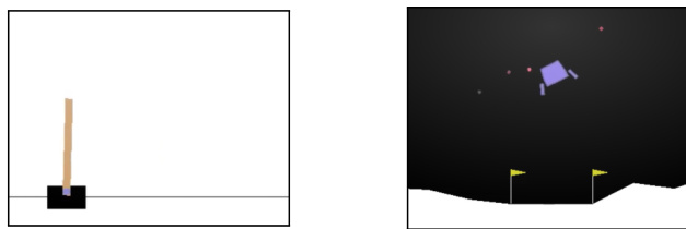
Figure 1: Screenshots of the classic control domains Cart Pole (left) and Lunar Lander (right)

图 1: 经典控制领域任务Cart Pole(左)和Lunar Lander(右)的界面截图

We can estimate (4) by sampling states from a trajectory and using function approximation:

我们可以通过从轨迹中采样状态并使用函数逼近来估计 (4) :

$$
\nabla_{\boldsymbol{\theta}}J(\boldsymbol{\theta})\approx\frac{1}{T}\sum_{t=0}^{T-1}\sum_{a\in\mathcal{A}}\nabla_{\boldsymbol{\theta}}\pi(a|s_{t};\boldsymbol{\theta})\widehat{Q}(s_{t},a;\omega).
$$

$$
\nabla_{\boldsymbol{\theta}}J(\boldsymbol{\theta})\approx\frac{1}{T}\sum_{t=0}^{T-1}\sum_{a\in\mathcal{A}}\nabla_{\boldsymbol{\theta}}\pi(a|s_{t};\boldsymbol{\theta})\widehat{Q}(s_{t},a;\omega).
$$

In our implementation, the inner summation is computed by combining two neural networks that represent the policy and state-action value function. The value function can be learned using a variety of methods, such as temporal-difference learning or Monte Carlo sampling. After performing a few updates to the value function, we update the parameters $\theta$ of the policy with the following update rule:

在我们的实现中，内部求和通过结合代表策略和状态-动作值函数的两个神经网络来计算。值函数可以通过多种方法学习，例如时序差分学习或蒙特卡洛采样。在对值函数进行几次更新后，我们使用以下更新规则来更新策略的参数 $\theta$：

$$
\theta\gets\theta+\alpha\sum_{t=0}^{T-1}\sum_{a\in\mathcal{A}}\nabla_{\theta}\pi(a|s_{t};\theta)\widehat{Q}(s_{t},a;\omega).
$$

$$
\theta\gets\theta+\alpha\sum_{t=0}^{T-1}\sum_{a\in\mathcal{A}}\nabla_{\theta}\pi(a|s_{t};\theta)\widehat{Q}(s_{t},a;\omega).
$$

To improve stability, repeated updates to the value and policy networks are interleaved, as in Generalized Policy Iteration (Sutton and Barto 1998).

为提高稳定性，我们对价值网络和策略网络进行交错重复更新，类似于广义策略迭代 (Sutton and Barto 1998) 的做法。

In traditional actor-critic approaches, which we refer to as sampled-action actor-critic, the only actions involved in the computation of the policy gradient estimate are those that were actually executed in the environment. In MAC, computing the policy gradient estimate will frequently involve actions that were not actually executed in the environment. This results in a trade-off between bias and variance. In domains where we can expect accurate Q-value predictions from our function approx im at or, despite not actually executing all of the relevant state-action pairs, MAC results in lower variance gradient updates and increased sample-efficiency. In domains where this assumption is not valid, MAC may perform worse than sampled-action actor-critic due to increased bias.

在传统的行动者-评论家方法（我们称之为采样行动行动者-评论家）中，参与策略梯度估计计算的动作仅限于那些实际在环境中执行的动作。而在MAC中，策略梯度估计的计算经常会涉及未实际执行的动作。这导致了偏差与方差之间的权衡。在我们能够从函数近似器中获得准确Q值预测的领域中，尽管并未实际执行所有相关的状态-动作对，MAC仍能实现更低方差的梯度更新和更高的样本效率。若这一假设不成立，由于偏差增加，MAC的表现可能不如采样行动行动者-评论家。

In some ways, MAC is similar to Expected Sarsa (Van Seijen et al. 2009). Expected Sarsa considers all next-actions $a_{t+1.}$ , then computes the expected TDerror, $\mathbb{E}[\delta]=~\dot{r}{t}+\gamma\mathbb{E}[Q(s_{t+1},a_{t+1})]-Q\dot{(}s_{t},a_{t}),$ and uses the resulting error signal to update the $Q$ function. By contrast, MAC considers all current-actions $^{a_{t},}$ and uses the corresponding $Q(s_{t},a_{t})$ values to update the policy directly.

在某些方面，MAC与Expected Sarsa (Van Seijen等人，2009)类似。Expected Sarsa考虑所有下一个动作$a_{t+1}$，然后计算期望TD误差$\mathbb{E}[\delta]=~\dot{r}{t}+\gamma\mathbb{E}[Q(s_{t+1},a_{t+1})]-Q\dot{(}s_{t},a_{t}),$并使用得到的误差信号更新$Q$函数。相比之下，MAC考虑所有当前动作$a_{t}$，并使用对应的$Q(s_{t},a_{t})$值直接更新策略。

It is natural to consider whether MAC could be improved by subtracting an action-independent baseline, as in sampled-action actor-critic and REINFORCE:

很自然地会考虑是否可以通过减去与动作无关的基线来改进MAC (Mean Actor-Critic) ，就像在采样动作演员-评论家 (sampled-action actor-critic) 和REINFORCE算法中那样：

$$
\nabla_{\boldsymbol{\theta}}J(\boldsymbol{\theta})=\underset{s\sim d^{\pi}}{\mathbb{E}}\Big[\sum_{\boldsymbol{a}\in\mathcal{A}}\nabla_{\boldsymbol{\theta}}\pi(\boldsymbol{a}|s;\boldsymbol{\theta})\Big(Q^{\pi}(s,\boldsymbol{a})-V^{\pi}(s)\Big)\Big].
$$

$$
\nabla_{\boldsymbol{\theta}}J(\boldsymbol{\theta})=\underset{s\sim d^{\pi}}{\mathbb{E}}\Big[\sum_{\boldsymbol{a}\in\mathcal{A}}\nabla_{\boldsymbol{\theta}}\pi(\boldsymbol{a}|s;\boldsymbol{\theta})\Big(Q^{\pi}(s,\boldsymbol{a})-V^{\pi}(s)\Big)\Big].
$$

However, we can simplify the expectation as follows:

然而，我们可以将期望简化为如下形式：

$$
\begin{array}{r l}&{\nabla_{\theta}J(\theta)=\underset{s\sim d^{\pi}}{\mathbb{E}}\Big[\underset{a\in\mathcal{A}}{\sum}\nabla_{\theta}\pi(a|s;\theta)Q^{\pi}(s,a)}\ &{\qquad-V^{\pi}(s)\nabla_{\theta}\underset{a\in\mathcal{A}}{\sum}\pi(a|s;\theta)\Big].}\end{array}
$$

$$
\begin{array}{r l}&{\nabla_{\theta}J(\theta)=\underset{s\sim d^{\pi}}{\mathbb{E}}\Big[\underset{a\in\mathcal{A}}{\sum}\nabla_{\theta}\pi(a|s;\theta)Q^{\pi}(s,a)}\ &{\qquad-V^{\pi}(s)\nabla_{\theta}\underset{a\in\mathcal{A}}{\sum}\pi(a|s;\theta)\Big].}\end{array}
$$

In doing so, we see that both $V^{\pi}(s)$ and the gradient operator can be moved outside of the summation, leaving just the sum of the action probabilities, which is always 1, and hence the gradient of the baseline term is always zero. This is true regardless of the choice of baseline, since the baseline cannot be a function of the actions or else it will bias the expectation. Thus, we see that subtracting a baseline is unnecessary in MAC, since it has no effect on the policy gradient estimate.

这样，我们发现$V^{\pi}(s)$和梯度算子都可以移到求和符号之外，剩下的只是动作概率之和（恒等于1），因此基线项的梯度始终为零。无论选择何种基线，这一结论都成立，因为基线不能是动作的函数，否则会偏置期望值。由此可见，在MAC中减去基线是多余的，因为它对策略梯度估计没有影响。

Analysis of Bias and Variance

偏差与方差分析

In this section we prove that MAC does not increase variance over sampled-action actor-critic (AC), and also, that given a fixed ${\widehat{Q}},$ both algorithms have the same bias. We start with tbhe bias result.

在本节中，我们证明MAC不会增加基于采样动作的演员-评论家(AC)方法的方差，并且给定固定的${\widehat{Q}}$时，两种算法具有相同的偏差。我们从偏差结果开始分析。

Theorem 1

定理 1

If the estimated Q-values, $\widehat{Q}(s,a;\omega)$ , for both MAC and AC are the same in ex pbectation, then the bias of MAC is equal to the bias of AC.

如果 MAC 和 AC 的估计 Q 值 $\widehat{Q}(s,a;\omega)$ 在期望上相同，那么 MAC 的偏差等于 AC 的偏差。

Proof

证明

See Appendix A.

见附录 A。

This result makes sense because in expectation, AC will choose all of the possible actions with some probability according to the policy. MAC simply calculates this expectation over actions explicitly. We now move to the variance result.

这一结果合乎预期，因为AC算法会依据策略以某种概率选择所有可能的动作。MAC则显式地计算了这些动作的期望值。接下来我们讨论方差结果。

Theorem 2

定理 2

If the estimated Q-values, $\widehat{Q}(s,a;\omega)$ , for both MAC and AC are the same in ex pebctation, and if $\widehat{Q}(s,a;\omega)$ is independent of $\widehat{Q}(s^{\prime},a^{\prime};\dot{\omega})$ for $(s,a)\neq(s^{\prime},a^{\prime})$ , then $\mathrm{Var}[\mathrm{M}\hat{\mathrm{A}}C]\leq\mathrm{Var}[\mathrm{AC}]$ . For deterministic policies, there is equality, and for stochastic policies the inequality is strict.

如果MAC和AC的估计Q值 $\widehat{Q}(s,a;\omega)$ 在期望上相同，且对于 $(s,a)\neq(s^{\prime},a^{\prime})$ ， $\widehat{Q}(s,a;\omega)$ 与 $\widehat{Q}(s^{\prime},a^{\prime};\dot{\omega})$ 相互独立，那么 $\mathrm{Var}[\mathrm{M}\hat{\mathrm{A}}C]\leq\mathrm{Var}[\mathrm{AC}]$ 。对于确定性策略，等式成立；对于随机策略，不等式严格成立。

Proof

证明

See Appendix B.

见附录 B。

Intuitively, we can see that for cases where the policy is deterministic, MAC’s formulation of the policy gradient is exactly equivalent to AC, and hence we can do no better than AC. For high-entropy policies, MAC will beat AC in terms of variance.

直观上可以看出，对于确定性策略的情况，MAC的策略梯度公式与AC完全等价，因此我们无法做得比AC更好。而对于高熵策略，MAC在方差方面会优于AC。

Algorithm	CartPole	LunarLander
REINFORCE	109.5±13.3	101.1 ±10.5
Adv.REINFORCE	121.8±11.2	114.7±8.1
Actor-Critic	138.7±13.2	124.6±5.1
Adv.Actor-Critic	157.4±6.4	162.8±14.9
MAC	178.3±7.6	163.5±12.8

算法	CartPole	LunarLander
REINFORCE	109.5±13.3	101.1±10.5
Adv.REINFORCE	121.8±11.2	114.7±8.1
Actor-Critic	138.7±13.2	124.6±5.1
Adv.Actor-Critic	157.4±6.4	162.8±14.9
MAC	178.3±7.6	163.5±12.8

Table 1: Performance summary of MAC vs. sampledaction policy gradient algorithms. Scores denote the mean performance of each algorithm over all trials and episodes.

表 1: MAC与抽样动作策略梯度算法的性能对比。分数表示各算法在所有试验和回合中的平均表现。

Experiments

实验

This section presents an empirical evaluation of MAC across three different problem domains. We first evaluate the performance of MAC versus popular policy gradient benchmarks on two classic control problems. We then evaluate MAC on a subset of Atari 2600 games and investigate its performance compared to state-ofthe-art policy search methods.

本节通过三个不同问题领域对MAC进行实证评估。我们首先在两个经典控制问题上比较MAC与主流策略梯度基准的性能表现。随后在Atari 2600游戏子集上评估MAC，并对比其与最先进策略搜索方法的性能表现。

Classic Control Experiments

经典控制实验

In order to determine whether MAC’s lower variance policy gradient estimate translates to faster learning, we chose two classic control problems, namely Cart Pole and Lunar Lander, and compared MAC’s performance against four standard sampled-action policy gradient algorithms. We used the open-source implementations of Cart Pole and Lunar Lander provided by OpenAI Gym (Brockman et al. 2016), in which both domains have continuous state spaces and discrete action spaces. Screenshots of the two domains are pro- vided in Figure 1.

为了验证MAC的低方差策略梯度估计是否能带来更快的收敛速度，我们选取了倒立摆(Cart Pole)和月球着陆器(Lunar Lander)两个经典控制问题，将MAC与四种标准采样动作策略梯度算法进行对比。实验采用OpenAI Gym (Brockman et al. 2016)提供的开源环境，这两个场景均具有连续状态空间和离散动作空间。图1展示了两个任务的界面截图。

For each problem domain, we implemented MAC using two independent neural networks, representing the policy and Q function. We then performed a hyper parameter search to determine the best network archi tec ture s, optimization method, and learning rates. Specifically, the hyper parameter search considered: 0, 1, 2, or 3 hidden layers; 50, 75, 100, or 300 neurons per layer; ReLU, Leaky ReLU (with leak factor 0.3), or tanh activation; SGD, RMSProp, Adam, or Adadelta as the optimization method; and a learning rate chosen from 0.0001, 0.00025, 0.0005, 0.001, 0.005, 0.01, or 0.05. To find the best setting, we ran 10 independent trials for each combination of hyper parameters and chose the setting with the best asymptotic performance over the 10 trials. We terminated each episode after 200 and 1000 timesteps (in Cart Pole and Lunar Lander, respectively), regardless of the state of the agent.

针对每个问题领域，我们采用两个独立的神经网络分别实现策略函数和Q函数的MAC系统。通过超参数搜索确定了最佳网络架构、优化方法和学习率。具体搜索范围包括：0/1/2/3个隐藏层；每层50/75/100/300个神经元；ReLU/Leaky ReLU(泄漏因子0.3)/tanh激活函数；SGD/RMSProp/Adam/Adadelta优化方法；以及从0.0001/0.00025/0.0005/0.001/0.005/0.01/0.05中选择学习率。每种超参数组合进行10次独立试验，选择10次试验中渐近性能最佳的组合。在Cart Pole和Lunar Lander环境中，分别设置200和1000个时间步长作为单次试验的终止条件，与智能体状态无关。

We compared MAC against four standard benchmarks: REINFORCE, advantage REINFORCE, actorcritic, and advantage actor-critic. We implemented the REINFORCE benchmarks using just a single neural network to represent the policy, and we implemented the actor-critic benchmarks using two networks to represent both the policy and Q function. For each benchmark algorithm, we then performed the same hyperparameter search that we had used for MAC.

我们将MAC与四种标准基准进行了比较：REINFORCE、优势REINFORCE、actor-critic以及优势actor-critic。我们仅使用单个神经网络来表示策略来实现REINFORCE基准，而actor-critic基准则采用两个网络分别表示策略和Q函数。针对每种基准算法，我们执行了与MAC相同的超参数搜索。

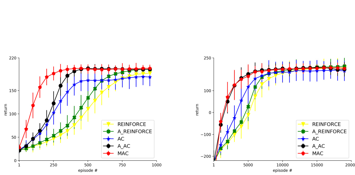
Figure 2: Performance comparison for CartPole (left) and Lunar Lander (right) of MAC vs. sampled-action policy gradient algorithms. Results are averaged over 100 independent trials.

图 2: MAC与采样动作策略梯度算法在CartPole(左)和Lunar Lander(右)任务上的性能对比。结果基于100次独立试验取平均值。

In order to keep the variance as low as possible for the advantage actor-critic benchmark, we explicitly computed the advantage function $A(s,a)=Q\dot{(}s,a)\stackrel{\smile}{-}$ $V(s)$ , where $\begin{array}{r}{V(s)=\sum_{a}\pi(a|s)Q(s,a).}\end{array}$ , rather than sampling it using the TD-error (see Section 2).

为了尽可能降低优势演员-评论家基准的方差，我们显式计算了优势函数 $A(s,a)=Q\dot{(}s,a)\stackrel{\smile}{-}$ $V(s)$ ，其中 $\begin{array}{r}{V(s)=\sum_{a}\pi(a|s)Q(s,a).}\end{array}$ ，而非使用TD误差进行采样(见第2节)。

Once we had determined the best hyper parameter settings for MAC and each of the benchmark algorithms, we then ran each algorithm for 100 independent trials. Figure 2 shows learning curves for the different algorithms, and Table 1 summarizes the results using the mean performance over trials and episodes. On Cart Pole, MAC learns substantially faster than all of the benchmarks, and on Lunar Lander, it performs competitively with the best benchmark algorithm, advantage actor-critic.

在确定MAC及各基准算法的最佳超参数设置后，我们对每个算法进行了100次独立试验。图2展示了不同算法的学习曲线，表1则汇总了各试验轮次和回合的平均性能结果。在Cart Pole任务中，MAC的学习速度显著快于所有基准算法；而在Lunar Lander任务中，其表现与最优基准算法优势行动者-评论家(advantage actor-critic)相当。

Atari Experiments

Atari 实验

To test whether MAC can scale to larger problem domains, we evaluated it on several Atari 2600 games using the Arcade Learning Environment (ALE) (Bellemare et al. 2013) and compared MAC’s performance against that of state-of-the-art policy search methods, namely, Trust Region Policy Optimization (TRPO) (Schulman et al. 2015), Evolutionary Strategies (ES) (Salimans et al. 2017), and Advantage Actor-Critic (A2C) (Wu et al. 2017). Due to the computational load inherent in training deep networks to play Atari games, we limited our experiments to a subset of six Atari games: Beamrider, Breakout, Pong, Q*bert, Seaquest and Space Invaders. These six games are commonly selected for tuning hyper parameters (Mnih et al. 2015; 2016; Wu et al. 2017), and thus provide a fair comparison against established benchmarks, despite our limited computational resources.

为测试MAC能否扩展到更大的问题领域，我们使用街机学习环境(ALE) (Bellemare et al. 2013)在多个Atari 2600游戏上评估其性能，并将MAC与最先进的策略搜索方法进行对比，包括信任域策略优化(TRPO) (Schulman et al. 2015)、进化策略(ES) (Salimans et al. 2017)和优势行动者-评论家(A2C) (Wu et al. 2017)。由于训练深度网络玩Atari游戏存在较高计算负荷，我们将实验限定在六个Atari游戏子集：Beamrider、Breakout、Pong、Q*bert、Seaquest和Space Invaders。这六款游戏常被用于超参数调优(Mnih et al. 2015; 2016; Wu et al. 2017)，因此即便在有限计算资源下，也能提供与既有基准的公平对比。

The MAC network architecture was derived from the OpenAI Baselines implementation of A2C (Wu et al. 2017). It uses three convolutional layers (size/stride/filters: 8/4/32, 4/2/64, 3/1/64), followed by a fully-connected layer (size 512), all with ReLU activation. A final fully-connected layer is split into two batches of N outputs each, where $_\mathrm{N}$ is the number of actions. One batch uses a linear activation and corresponds to the $\mathrm{Q}$ -values; the other batch uses a softmax activation and corresponds to the policy. We used this architecture for both the MAC results and the A2C results. The TRPO and ES results are taken from their respective papers.

MAC网络架构源自OpenAI Baselines对A2C的实现(Wu et al. 2017)。该架构包含三个卷积层(尺寸/步长/滤波器数: 8/4/32、4/2/64、3/1/64)，后接一个全连接层(尺寸512)，所有层均采用ReLU激活函数。最后的全连接层被分割为两组各N个输出(其中$_\mathrm{N}$表示动作数量)：一组采用线性激活函数对应$\mathrm{Q}$值，另一组采用softmax激活函数对应策略函数。我们在MAC和A2C实验结果中均采用此架构，TRPO与ES结果则分别引自其原始论文。

We trained the network using a variation of the multi-part loss function used in A2C (Wu et al. 2017). The value loss at each timestep was equal to the mean squared error between the observed reward and the Q-value of the selected action. The policy entropy loss was simply the negative entropy of the policy at each timestep. For the A2C experiments, the policy improvement loss was the negative log probability of the selected action times its advantage value. For the MAC experiments, the policy improvement loss became the negative sum of action probabilities times their associated $\mathrm{Q}.$ -values. The overall loss function was a linear combination of the policy improvement loss (coefficient 0.1), policy entropy loss (coefficient 0.001), and value loss (coefficient 0.5), and the network was trained using RMSProp with a learning rate of 1.5e3. These coefficients trade off the importance of learning good Q-values, improving the policy, and preventing the policy from converging prematurely. This configuration of hyper parameters was found to perform well experimentally for both methods after a small hyper parameter search. The only difference between the A2C and MAC implementations was to replace A2C’s sampled-action policy improvement loss with MAC’s sum-over-actions loss; the algorithms used exactly the same architecture and hyper parameters.

我们采用A2C (Wu et al. 2017) 中使用的多部分损失函数的变体来训练网络。每个时间步的价值损失等于观察到的奖励与所选动作Q值之间的均方误差。策略熵损失仅是每个时间步策略的负熵。在A2C实验中，策略改进损失是所选动作的负对数概率乘以其优势值。对于MAC实验，策略改进损失变为动作概率与其关联$\mathrm{Q}$值的负和。整体损失函数是策略改进损失（系数0.1）、策略熵损失（系数0.001）和价值损失（系数0.5）的线性组合，网络使用RMSProp进行训练，学习率为1.5e3。这些系数权衡了学习良好Q值、改进策略和防止策略过早收敛的重要性。经过少量超参数搜索后，发现这种超参数配置在两种方法中均表现良好。A2C和MAC实现之间的唯一区别是将A2C的采样动作策略改进损失替换为MAC的动作求和损失；两种算法使用完全相同的架构和超参数。

Table 2: Atari performance of MAC vs. policy search methods (random start condition). TRPO and ES results are from their respective papers (Schulman et al. 2015; Salimans et al. 2017). A2C and MAC results were obtained with modified versions of the OpenAI Baselines implementation of A2C (Wu et al. 2017).

Game	Random	TRPO	ES	A2C	MAC
BeamRider	363.9	1425.2	744.0	5846.0	6072.0
Breakout	1.7	10.8	9.5	370.9	372.7
Pong	-20.7	20.9	21.0	18.0	10.6
Q*bert	183.0	1973.5	147.5	1651.5	243.4
Seaquest	68.4	1908.6	1390.0	1702.5	1703.4
Space Invaders	148.0	568.4	678.5	1201.2	1173.1

表 2: MAC与策略搜索方法在Atari游戏中的性能对比(随机起始条件)。TRPO和ES的结果分别来自其原始论文(Schulman et al. 2015; Salimans et al. 2017)。A2C和MAC的结果是通过修改OpenAI Baselines中A2C的实现版本(Wu et al. 2017)获得的。

游戏	随机	TRPO	ES	A2C	MAC
BeamRider	363.9	1425.2	744.0	5846.0	6072.0
Breakout	1.7	10.8	9.5	370.9	372.7
Pong	-20.7	20.9	21.0	18.0	10.6
Q*bert	183.0	1973.5	147.5	1651.5	243.4
Seaquest	68.4	1908.6	1390.0	1702.5	1703.4
Space Invaders	148.0	568.4	678.5	1201.2	1173.1

For A2C and MAC, we trained a network for each game on 50 million frames of play, across 16 parallel threads, pausing every 200K frames to evaluate performance and compute learning curves. In each evaluation, we ran 16 agents in parallel, for 4500 frames (5 minutes) each, or 50 total episodes, whichever came first, and averaged the scores of the completed (or timed-out) episodes. Agents were trained and evaluated under the typical random start condition, where the game is initialized with a random number of no-op ALE actions (between 0 and 30) (Mnih et al. 2015). The A2C and MAC results in Table 2 come from the final evaluation after all 50M frames, and they are averaged across 5 trials involving separately trained networks. Learning curves for each game can be found in Figure in the Appendix. In addition to A2C, we also compared MAC against TRPO (results from a single trial) (Schulman et al. 2015), and ES (results averaged over 30 trials) (Salimans et al. 2017), and found that MAC performed competitively with all three benchmark algorithms.

对于A2C和MAC，我们在16个并行线程上为每个游戏训练了5000万帧的网络，每20万帧暂停一次以评估性能并计算学习曲线。每次评估时，我们并行运行16个智能体，每个运行4500帧（5分钟）或50个完整回合（以先达到者为准），并计算已完成（或超时）回合的平均得分。智能体的训练和评估均在典型的随机起始条件下进行，即游戏初始化时会执行0到30次随机无操作ALE动作 (Mnih et al. 2015)。表2中的A2C和MAC结果来自5000万帧训练后的最终评估，且为5次独立训练网络试验的平均值。各游戏的学习曲线详见附录中的图。除A2C外，我们还将MAC与TRPO（单次试验结果）(Schulman et al. 2015)和ES（30次试验平均值）(Salimans et al. 2017)进行对比，发现MAC与这三种基准算法相比具有竞争力。

Note that MAC’s performance on Pong and Q*bert was low relative to A2C. For Pong this was due to one of the five MAC trials obtaining a final score of -20.1 and pulling the average performance down significantly. The individual Pong scores for MAC were ${20.5,1\dot{9}.7,18.3,14.7,-20.1}$ ; the scores for A2C were ${19.4,19.4,19.3,16.3,15.6}$ . For Q*bert, the performance for both algorithms was much more variable. A2C scored 0.0 on 3 out of 5 trials, and MAC scored 0.0 on 2 out of 5 trials. The reason A2C’s average score is so much higher than MAC’s is that it had one lucky trial where it scored 7780.9 points. The individual ${\dot{Q}}^{*}$ bert scores for MAC were ${557.4,504.7,155.1,0.0,0.0}.$ ; the scores for A2C were ${7780.9,476.6,0.0,0.0,0.0}$ . Additional hyper parameter tuning might lead to improved performance; however, the purpose of this Atari experiment was mainly to show that MAC is competitive with state-of-the-art policy search algorithms, and these results seem to indicate that it is.

注意到MAC在《Pong》和《Qbert》上的表现相对于A2C较低。对于《Pong》，这是由于五次MAC试验中有一个最终得分为-20.1，显著拉低了平均表现。MAC在《Pong》中的具体得分为${20.5,1\dot{9}.7,18.3,14.7,-20.1}$，而A2C的得分为${19.4,19.4,19.3,16.3,15.6}$。对于《Qbert》，两种算法的表现波动更大。A2C在五次试验中有三次得分为0.0，而MAC在五次试验中有两次得分为0.0。A2C平均得分远高于MAC的原因是其有一次幸运的试验获得了7780.9分。MAC在《Q*bert》中的具体得分为${557.4,504.7,155.1,0.0,0.0}$，而A2C的得分为${7780.9,476.6,0.0,0.0,0.0}$。进一步的超参数调整可能会提升表现，但本次Atari实验的主要目的是展示MAC与最先进的策略搜索算法具有竞争力，而这些结果似乎表明了这一点。

Discussion

讨论

At its core, MAC offers a new way of computing the policy gradient that can substantially reduce variance and increase learning speed. There are a number of orthogonal improvements to policy gradient methods, such as using natural gradients (Kakade 2002; Peters and Schaal 2008), off-policy learning (Wang et al. 2016; Gu et al. 2016; Asadi and Williams 2016), secondorder methods (Furmston, Lever, and Barber 2016), and asynchronous exploration (Mnih et al. 2016). We have not investigated how MAC performs with these extensions; however, just as these improvements were added to basic actor-critic methods, they could be added to MAC as well, and we expect they would improve its performance in a similar way.

MAC 的核心在于提供了一种计算策略梯度 (policy gradient) 的新方法，能显著降低方差并提高学习速度。策略梯度方法存在许多正交改进方向，例如使用自然梯度 (Kakade 2002; Peters and Schaal 2008)、离策略学习 (Wang et al. 2016; Gu et al. 2016; Asadi and Williams 2016)、二阶方法 (Furmston, Lever, and Barber 2016) 以及异步探索 (Mnih et al. 2016)。我们尚未研究 MAC 如何与这些扩展结合使用；然而，正如这些改进被应用于基础的行动者-评论家 (actor-critic) 方法一样，它们也可以被整合到 MAC 中，我们预期它们会以类似的方式提升其性能。

A typical use-case for actor-critic algorithms is for problem domains with continuous actions, which are awkward for value-function-based methods (Sutton and Barto 1998). One approach to dealing with continuous actions is Deterministic Policy Gradients (DPG) (Silver et al. 2014; Lillicrap et al. 2015), which uses a determini stic policy to perform off-policy policy gradient updates. However, in settings where on-policy learning is necessary, using a deterministic policy leads to sub-optimal behavior (Sutton and Barto 1998), and hence a stochastic policy is typically used instead. The recently-introduced Expected Policy Gradients (EPG) (Ciosek and Whiteson 2017) addresses this problem by generalizing DPG for stochastic policies. However, while EPG has good experimental performance on domains with continuous action spaces, the authors do not provide experimental results for discrete domains. MAC’s discrete results and EPG’s continuous results are in some sense complementary.

演员-评论家 (actor-critic) 算法的典型应用场景是针对具有连续动作的问题领域，这对基于价值函数的方法来说较为棘手 (Sutton and Barto 1998)。处理连续动作的一种方法是确定性策略梯度 (Deterministic Policy Gradients, DPG) (Silver et al. 2014; Lillicrap et al. 2015)，它使用确定性策略执行离策略 (off-policy) 的策略梯度更新。然而，在需要同策略 (on-policy) 学习的场景中，使用确定性策略会导致次优行为 (Sutton and Barto 1998)，因此通常会改用随机策略。最近提出的期望策略梯度 (Expected Policy Gradients, EPG) (Ciosek and Whiteson 2017) 通过将 DPG 推广到随机策略来解决这个问题。不过，尽管 EPG 在连续动作空间领域表现出良好的实验性能，作者并未提供离散领域的实验结果。MAC 的离散结果与 EPG 的连续结果在某种意义上具有互补性。

Conclusion

结论

The basic formulation of policy gradient estimators presented here—where the gradient is estimated by averaging the state-action value function across actions—leads to a new family of actor-critic algorithms. This family has the advantage of not requiring an additional variance-reduction baseline, sub- stantially reducing the design effort required to apply them. It is also a natural fit with deep neural network function ap proxima tors, resulting in a network architecture that is identical to some sampled-action actorcritic algorithms, but with less variance.

这里介绍的政策梯度估计器基本公式——通过平均动作的状态-动作价值函数来估计梯度——催生了一个新的行动者-评论家 (actor-critic) 算法家族。该家族的优势在于无需额外的方差缩减基线，大幅降低了应用所需的设计工作量。它还能与深度神经网络函数逼近器自然契合，形成与某些采样动作行动者-评论家算法相同的网络架构，但方差更小。

Figure 3: Learning curves on six Atari games for A2C (blue) and MAC (orange). Vertical axis is score; horizontal axis is number of training frames (in millions). Results are averaged over 5 independent trials, and smoothed slightly for readability. Error bars represent standard deviation.

图 3: A2C (蓝色) 和 MAC (橙色) 在六款 Atari 游戏上的学习曲线。纵轴为得分；横轴为训练帧数 (单位：百万)。结果为 5 次独立试验的平均值，并经过轻微平滑处理以提高可读性。误差条表示标准差。

We prove that for stochastic policies, the MAC algorithm (the simplest member of the resulting family), reduces variance relative to traditional actor-critic approaches, while maintaining the same bias. Our neural network implementation of MAC either outperforms, or is competitive with, state-of-the-art policy search algorithms, and our experimental results show that MAC’s lower variance lead to dramatically faster training in some cases. In future work, we aim to develop this family of algorithms further by including typical elaborations of the basic actor-critic architecture like natural or second-order gradients. Our results so far suggest that our new approach is highly promising, and that extensions to it will provide even further improvement in performance.

我们证明，对于随机策略，MAC算法（该算法家族中最简单的成员）在保持相同偏差的同时，相比传统行动者-评论家方法降低了方差。我们的MAC神经网络实现要么优于、要么可与最先进的策略搜索算法相媲美，实验结果表明MAC的较低方差在某些情况下能显著加快训练速度。未来工作中，我们计划通过融入自然梯度或二阶梯度等典型行动者-评论家架构改进方案，进一步扩展该算法家族。目前结果表明我们的新方法极具前景，其扩展版本将带来更优异的性能表现。

References

参考文献

Wu, Y.; Mansimov, E.; Grosse, R. B.; Liao, S.; and Ba,J. 2017. Scalable trust-region method for deep reinforcement learning using kronecker-factored approximation. In Advances in neural information processing systems, 5285–5294.

Wu, Y.; Mansimov, E.; Grosse, R. B.; Liao, S.; and Ba, J. 2017. 使用克罗内克分解近似的可扩展信任域深度强化学习方法。In Advances in neural information processing systems, 5285–5294.

Appendix

附录

A. Proof of Theorem 1

A. 定理1的证明

Both AC and MAC are estimators of the true policy gradient (PG). Given a batch of data $D$ , we can write the bias of AC and MAC as:

AC和MAC都是真实策略梯度(PG)的估计器。给定一批数据$D$，我们可以将AC和MAC的偏差表示为：

$$
{\begin{array}{r l}{\mathrm{Bias}[\mathrm{AC}]=}&{\mathbb{E}_{_D}[A C]-\mathrm{PG}}\ {\mathrm{Bias}[\mathrm{MAC}]=}&{\mathbb{E}_{_D}[M A C]-\mathrm{PG}}\end{array}}
$$

$$
{\begin{array}{r l}{\mathrm{Bias}[\mathrm{AC}]=}&{\mathbb{E}_{_D}[A C]-\mathrm{PG}}\ {\mathrm{Bias}[\mathrm{MAC}]=}&{\mathbb{E}_{_D}[M A C]-\mathrm{PG}}\end{array}}
$$

For clarity, we will rewrite the AC and MAC expectations (1) and (4) to explicitly denote the way that each algorithm estimates the policy gradient, given a batch of data $D$ (with size $|D|.$ ):

为明确起见，我们将重写AC和MAC的期望(1)和(4)，以显式表示每种算法在给定数据批次$D$（大小为$|D|$）时对策略梯度的估计方式：

$$
\begin{array}{l}{\displaystyle\mathrm{AC}=\frac{1}{|D|}\sum_{(s,a)\in D}\nabla_{\theta}\log\pi(a|s;\theta)\widehat{Q}(s,a;\omega)}\ {\displaystyle\mathrm{MAC}=\frac{1}{|D|}\sum_{s\in D}\sum_{a\in\mathcal{A}}\pi(a|s;\theta)\nabla_{\theta}\log\pi(a|s;\theta)\widehat{Q}(s,a;\omega)}\end{array}
$$

Substituting (8) and (1) into Eqn. (6) gives:

将式(8) 和式(1) 代入式(6) 可得:

$$
\mathrm{Bias}[\mathrm{AC}]=\mathbb{E}{\boldsymbol{D}}\left[\frac{1}{|\boldsymbol{D}|}\sum_{t=1}^{|D|}\nabla_{\theta}\log\pi(a_{t}|s_{t};\theta)\widehat{Q}(s_{t},a_{t};\omega)\right]-\underbrace{\mathbb{E}}{s\sim d^{\pi},a\sim\pi}\left[\nabla_{\theta}\log\pi(a|s;\theta)Q^{\pi}(s,a)\right].
$$

$$
\mathrm{Bias}[\mathrm{AC}]=\mathbb{E}{\boldsymbol{D}}\left[\frac{1}{|\boldsymbol{D}|}\sum_{t=1}^{|D|}\nabla_{\theta}\log\pi(a_{t}|s_{t};\theta)\widehat{Q}(s_{t},a_{t};\omega)\right]-\underbrace{\mathbb{E}}{s\sim d^{\pi},a\sim\pi}\left[\nabla_{\theta}\log\pi(a|s;\theta)Q^{\pi}(s,a)\right].
$$

Since $D$ is sampled from trajectories that were carried out according to the policy, we can drop the dependence on $t$ inside the expectation, and rewrite (10) as follows:

由于 $D$ 是从根据策略执行的轨迹中采样的，我们可以去掉期望中对 $t$ 的依赖，并将 (10) 重写如下：

$$
\begin{array}{r l}&{\mathrm{iias}[\mathrm{AC}]=\frac{1}{|D|}\displaystyle\sum_{t=1}^{|D|}\Big(_{s\sim d^{\pi},a\sim\pi}\Big[\nabla_{\theta}\log\pi(a|s;\theta)\widehat{Q}(s,a;\omega)\Big]\Big)-\underset{s\sim d^{\pi},a\sim\pi}{\mathbb{E}}\Big[\nabla_{\theta}\log\pi(a|s;\theta)Q^{\pi}(s,a;\omega)\Big]}\ &{\quad\quad\quad=\underset{s\sim d^{\pi},a\sim\pi}{\mathbb{E}}\Big[\nabla_{\theta}\log\pi(a|s;\theta)\Big(\widehat{Q}(s,a;\omega)-Q^{\pi}(s,a)\Big)\Big]}\ &{\quad\quad\quad=\underset{s\sim d^{\pi}}{\mathbb{E}}\Big[\sum_{a\in A}\pi(a|s;\theta)\nabla_{\theta}\log\pi(a|s;\theta)\Big(\widehat{Q}(s,a;\omega)-Q^{\pi}(s,a)\Big)\Big]}\end{array}
$$

$$
\begin{array}{r l}&{\mathrm{iias}[\mathrm{AC}]=\frac{1}{|D|}\displaystyle\sum_{t=1}^{|D|}\Big(_{s\sim d^{\pi},a\sim\pi}\Big[\nabla_{\theta}\log\pi(a|s;\theta)\widehat{Q}(s,a;\omega)\Big]\Big)-\underset{s\sim d^{\pi},a\sim\pi}{\mathbb{E}}\Big[\nabla_{\theta}\log\pi(a|s;\theta)Q^{\pi}(s,a;\omega)\Big]}\ &{\quad\quad\quad=\underset{s\sim d^{\pi},a\sim\pi}{\mathbb{E}}\Big[\nabla_{\theta}\log\pi(a|s;\theta)\Big(\widehat{Q}(s,a;\omega)-Q^{\pi}(s,a)\Big)\Big]}\ &{\quad\quad\quad=\underset{s\sim d^{\pi}}{\mathbb{E}}\Big[\sum_{a\in A}\pi(a|s;\theta)\nabla_{\theta}\log\pi(a|s;\theta)\Big(\widehat{Q}(s,a;\omega)-Q^{\pi}(s,a)\Big)\Big]}\end{array}
$$

Now we turn our attention to MAC, and substitute (9) and (1) into Eqn. (7), to obtain:

现在我们将注意力转向MAC，并将(9)和(1)代入方程(7)，得到：

$$
\begin{array}{r l}{\mathrm{ias}[\mathbf{MAC}]=}&{\mathbb{E}{{D}}\left[\frac{1}{|D|}\displaystyle\sum_{t=1}^{D|}\sum_{a\in{\mathcal{A}}}\pi(a|s_{t};\theta)\nabla_{\theta}\log\pi(a|s_{t};\theta)\widehat{Q}(s_{t},a;\omega)\right]-\underset{s\sim d^{T},a\sim\pi}{\mathbb{E}}\left[\nabla_{\theta}\log\pi(a|s;\theta)\widehat{Q}(s_{t},a;\omega)\right]}\ &{=\frac{1}{|D|}\displaystyle\sum_{t=1}^{D|}\sum_{s\sim d^{\pi}}\Big[\sum_{a\in{\mathcal{A}}}\pi(a|s;\theta)\nabla_{\theta}\log\pi(a|s;\theta)\widehat{Q}(s,a;\omega)\Big]-\underset{s\sim d^{\pi}}{\mathbb{E}}\left[\nabla_{\theta}\log\pi(a|s;\theta)\widehat{Q}(s,a;\omega)\right]}\ &{=\underset{s\sim d^{\pi}}{\mathbb{E}}\left[\sum_{a\in{\mathcal{A}}}\pi(a|s;\theta)\nabla_{\theta}\log\pi(a|s;\theta)\widehat{Q}(s,a;\omega)\right]-\underset{s\sim d^{\pi}}{\mathbb{E}}\left[\sum_{a\in{\mathcal{A}}}\pi(a|s;\theta)\nabla_{\theta}\log\pi(a|s;\theta)\widehat{Q}(s,a;\omega)\right]}\ &{=\underset{s\sim d^{\pi}}{\mathbb{E}}\left[\sum_{a\in{\mathcal{A}}}\pi(a|s;\theta)\nabla_{\theta}\log\pi(a|s_{t};\theta)\left(\widehat{Q}(s,a;\omega)-Q^{\pi}(s,a)\right)\right]}\end{array}
$$

Comparing (13) and (17), we see that AC and MAC have the same bias.

比较 (13) 和 (17) 可知，AC 和 MAC 具有相同的偏差。

B. Proof of Theorem 2

B. 定理2的证明

For any random variable $Z_{.}$ , the variance $\mathrm{Var}[Z]$ can be written as:

对于任意随机变量 $Z_{.}$，其方差 $\mathrm{Var}[Z]$ 可表示为：

$$
\mathrm{Var}[Z]=\mathbb{E}\left[Z^{2}\right]-\mathbb{E}[Z]^{2}
$$

$$
\mathrm{Var}[Z]=\mathbb{E}\left[Z^{2}\right]-\mathbb{E}[Z]^{2}
$$

If we assume the estimated Q-values for MAC and AC are the same in expectation, then the squared expectation’s contribution to the variance of each algorithm will be equal. We are only interested in determining which estimator has lower variance, so we can drop the second term and simply compare $\mathbb{E}\left[Z^{2}\right]$ , the second moments.

如果我们假设MAC和AC的估计Q值在期望上相同，那么平方期望对每个算法方差的贡献将是相等的。我们只关心确定哪个估计器的方差更低，因此可以舍弃第二项，直接比较二阶矩$\mathbb{E}\left[Z^{2}\right]$。

Again we will employ the explicit definitions of the AC and MAC estimators, for a data set $D$ , given by (8) and (9), respectively.

我们将再次采用AC和MAC估计量的显式定义，对于数据集$D$，分别由(8)和(9)给出。

For ease of notation, we define the following two functions:

为便于表述，我们定义以下两个函数：

$$
\begin{array}{l}{{X(s,a)=\nabla_{\theta_{i}}\log\pi(a|s;\theta)\widehat{Q}(s,a;\omega)}}\ {{Y(s)=\displaystyle\mathbb{E}_{\pi}\left[X(s,a)\right]=\sum_{a\in U(s)}\pi(a|s;\theta)X(s,a)}}\end{array}
$$

$$
\begin{array}{l}{{X(s,a)=\nabla_{\theta_{i}}\log\pi(a|s;\theta)\widehat{Q}(s,a;\omega)}}\ {{Y(s)=\displaystyle\mathbb{E}_{\pi}\left[X(s,a)\right]=\sum_{a\in U(s)}\pi(a|s;\theta)X(s,a)}}\end{array}
$$

Here, $\theta_{i}$ represents a single parameter of the parameter vector $\theta$ . We consider an arbitrary choice of $i,$ so the following proof holds for all $i$ .

这里，$\theta_{i}$ 表示参数向量 $\theta$ 的单个参数。我们考虑任意选择的 $i$，因此以下证明对所有 $i$ 都成立。

The above expressions allow us to rewrite the AC and MAC estimators (Eqn. 8 & 9) in terms of $X(s,a)$ and $Y(s)$ :

上述表达式允许我们用$X(s,a)$和$Y(s)$重写AC和MAC估计量(式8和9):

$$
\begin{array}{c}{\displaystyle\mathrm{AC}{i}=\frac{1}{|D|}\sum_{(s,a)\in D}X(s,a)}\ {\displaystyle\mathrm{MAC}{i}=\frac{1}{|D|}\sum_{s\in D}\sum_{a\in U(s)}Y(s)}\end{array}
$$

$$
\begin{array}{c}{\displaystyle\mathrm{AC}{i}=\frac{1}{|D|}\sum_{(s,a)\in D}X(s,a)}\ {\displaystyle\mathrm{MAC}{i}=\frac{1}{|D|}\sum_{s\in D}\sum_{a\in U(s)}Y(s)}\end{array}
$$

For convenience, we drop the $i$ subscript for the rest of this analysis.

为方便起见，我们在后续分析中省略下标$i$。

Now we are ready to compare $\mathbb{E}{s,a}[\mathrm{AC}^{2}]$ vs. $\mathbb{E}_{s}[\mathrm{MAC}^{2}]$ .

现在我们准备比较 $\mathbb{E}{s,a}[\mathrm{AC}^{2}]$ 和 $\mathbb{E}{s}[\mathrm{MAC}^{2}]$。
By the assumption that $\widehat{Q}(s,a;\omega)$ is independent of $\widehat{Q}(s^{\prime},a^{\prime};\omega)$ for $(s,a)\neq(s^{\prime},a^{\prime}),$ we can distribute the expectation through $\mathbb{E}[X(s,a)X(s^{\prime},a^{\prime})]$ in line 3 on the left, to obbtain $\mathbb{E}[X(s,a)]\operatorname{\mathbb{E}}[X(s^{\prime},a^{\prime})]$ . In the last line, we can drop the second term in each expression, because they are the same. At this point we just need to compare $\mathbb{E}{s,a}[X(s,a)^{2})]$ vs. $\mathbb{E}_{s}[Y(s)^{2}]$ . In order to make this comparison, we make use of Jensen’s Inequality (Jensen 1906), which says that for a convex function $f$ and a vector $Z\in\mathbb{R}^{n}$ :

根据假设 $\widehat{Q}(s,a;\omega)$ 与 $\widehat{Q}(s^{\prime},a^{\prime};\omega)$ 在 $(s,a)\neq(s^{\prime},a^{\prime})$ 时相互独立，我们可以将左侧第3行的期望 $\mathbb{E}[X(s,a)X(s^{\prime},a^{\prime})]$ 分解为 $\mathbb{E}[X(s,a)]\operatorname{\mathbb{E}}[X(s^{\prime},a^{\prime})]$。最后一行中，由于各项第二项相同，可以将其省略。此时只需比较 $\mathbb{E}{s,a}[X(s,a)^{2})]$ 与 $\mathbb{E}_{s}[Y(s)^{2}]$。为此，我们运用Jensen不等式 (Jensen 1906)：对于凸函数 $f$ 和向量 $Z\in\mathbb{R}^{n}$，有：

$$
\mathbb{E}[f(Z)]\ge f(\mathbb{E}[Z])
$$

$$
\mathbb{E}[f(Z)]\ge f(\mathbb{E}[Z])
$$

We note that $f(z)=z^{2}$ is convex, and as such, the following holds:

我们注意到 $f(z)=z^{2}$ 是凸函数，因此以下结论成立：

$$
\forall_{s}\operatorname{\mathbb{E}}[X(s,a)^{2}]\geq(\operatorname{\mathbb{E}}[X(s,a)])^{2}\implies\forall_{s}\operatorname{\mathbb{E}}[X(s,a)^{2}]\geq Y(s)^{2}\implies\operatorname{\mathbb{E}}_{s,a}[X(s,a)^{2}]\geq\operatorname{\mathbb{E}}[Y(s)^{2}]
$$

$$
\forall_{s}\operatorname{\mathbb{E}}[X(s,a)^{2}]\geq(\operatorname{\mathbb{E}}[X(s,a)])^{2}\implies\forall_{s}\operatorname{\mathbb{E}}[X(s,a)^{2}]\geq Y(s)^{2}\implies\operatorname{\mathbb{E}}_{s,a}[X(s,a)^{2}]\geq\operatorname{\mathbb{E}}[Y(s)^{2}]
$$

Thus, we can conclude that $\mathrm{Var}[\mathrm{MAC}]\leq\mathrm{Var}[\mathrm{AC}]$ . Moreover, since $f(z)=z^{2}$ is strictly convex, this inequality is strict as long as $a$ is not almost surely constant for a given state. That means for deterministic policies, we have $\mathrm{Var}[\mathrm{MAC}]\stackrel{\sim}{=}\mathrm{Var}[\mathrm{AC}],$ , and for stochastic policies, $\mathrm{Var}[\mathrm{MAC}]<\mathrm{Var}[\mathrm{AC}]$ .

因此，我们可以得出结论：$\mathrm{Var}[\mathrm{MAC}]\leq\mathrm{Var}[\mathrm{AC}]$。此外，由于 $f(z)=z^{2}$ 是严格凸函数，只要给定状态下 $a$ 不是几乎必然为常数，该不等式严格成立。这意味着对于确定性策略，有 $\mathrm{Var}[\mathrm{MAC}]\stackrel{\sim}{=}\mathrm{Var}[\mathrm{AC}]$；而对于随机策略，则满足 $\mathrm{Var}[\mathrm{MAC}]<\mathrm{Var}[\mathrm{AC}]$。