GAN-based Anomaly Detection in Imbalance Problems
基于GAN的不平衡问题异常检测
Abstract. Imbalance problems in object detection are one of the key issues that affect the performance greatly. Our focus in this work is to address an imbalance problem arising from defect detection in industrial inspections, including the different number of defect and non-defect dataset, the gap of distribution among defect classes, and various sizes of defects. To this end, we adopt the anomaly detection method that is to identify unusual patterns to address such challenging problems. Especially generative adversarial network (GAN) and auto encoder-based approaches have shown to be effective in this field. In this work, 1) we propose a novel GAN-based anomaly detection model which consists of an auto encoder as the generator and two separate disc rim in at or s for each of normal and anomaly input; and 2) we also explore a way to effectively optimize our model by proposing new loss functions: Patch loss and Anomaly adversarial loss, and further combining them to jointly train the model. In our experiment, we evaluate our model on conventional benchmark datasets such as MNIST, Fashion MNIST, CIFAR 10/100 data as well as on real-world industrial dataset – smartphone case defects. Finally, experimental results demonstrate the effectiveness of our approach by showing the results of outperforming the current State-OfThe-Art approaches in terms of the average area under the ROC curve (AUROC).
摘要。目标检测中的不平衡问题是严重影响性能的关键因素之一。本研究重点解决工业检测中缺陷检测引发的三类不平衡问题:缺陷与非缺陷数据集的数量差异、缺陷类别间的分布差距以及缺陷尺寸的多样性。为此,我们采用识别异常模式的异常检测方法应对这些挑战。其中,基于生成对抗网络 (GAN) 和自动编码器的方法已在该领域展现出显著效果。本研究贡献包括:1) 提出新型GAN异常检测模型,采用自动编码器作为生成器,并分别为正常/异常输入配置独立判别器;2) 通过提出Patch loss和Anomaly adversarial loss两种新损失函数,探索模型优化路径,并实现联合训练。实验环节在MNIST、Fashion MNIST、CIFAR 10/100等基准数据集及智能手机外壳缺陷真实工业数据集上进行验证。最终,ROC曲线下平均面积 (AUROC) 指标显示,本方法性能优于当前最优方案。
1 Introduction
1 引言
The importance of the imbalance problems in machine learning is investigated widely and many researches have been trying to solve them [12],[20],[23],[28],[34]. For example, class imbalance in the dataset can dramatically skew the performance of class if i ers, introducing a prediction bias for the majority class [23]. Not only class imbalance, but various imbalance problems exist in data science. A general overview of imbalance problems is investigated in the literature [12],[20],[23],[28]. Specifically, the survey of various imbalance problems for object detection subject is described in the review paper [34].
机器学习中不平衡问题的重要性已被广泛研究,许多学者致力于解决此类问题 [12]、[20]、[23]、[28]、[34]。例如,数据集中的类别不平衡会显著扭曲分类器的性能,导致对多数类的预测偏差 [23]。数据科学领域不仅存在类别不平衡,还存在多种其他不平衡问题。文献 [12]、[20]、[23]、[28] 对不平衡问题进行了全面综述。具体而言,综述论文 [34] 详细探讨了目标检测领域中的各类不平衡问题。
We handle a couple of imbalance problems closely related to industrial defects detection in this paper. Surface defects of metal cases such as scratch, stamped, and stain are very unlikely to happen in the production process, thereby resulting in outstanding class imbalance. Besides, size of defects, loss scale, and disc rim in at or distribution al imbalances are covered as well. In order to prevent such imbalance problems, anomaly detection [8] approach is used. This method discards a small portion of the sample data and converts the problem into an anomaly detection framework. Considering the shortage and diversity of anomalous data, anomaly detection is usually modeled as a one-class classification problem, with the training dataset containing only normal data [40].
本文重点解决与工业缺陷检测密切相关的几类不平衡问题。金属外壳表面缺陷(如划痕、压痕、污渍)在生产过程中极少出现,导致严重的类别不平衡。此外,我们还涵盖了缺陷尺寸、损失量级以及盘缘分布不平衡等问题。为防止此类不平衡问题,采用异常检测[8]方法,该方法通过舍弃少量样本数据将问题转化为异常检测框架。鉴于异常数据的稀缺性和多样性,异常检测通常被建模为单分类问题,训练数据集仅包含正常数据[40]。
Reconstruction-based approaches [1],[41],[43] have been paid attention for anomaly detection. The idea behind this is that auto encoders can reconstruct normal data with small errors, while the reconstruction errors of anomalous data are usually much larger. Auto encoder [33] is adopted by most reconstructionbased methods which assume that normal and anomalous samples could lead to significantly different embeddings and thus differences in the corresponding reconstruction errors can be leveraged to differentiate the two types of samples [42]. Adversarial training is introduced by adding a disc rim in at or after auto encoders to judge whether its original or reconstructed image [10],[41]. Schlegl et al. [43] hypothesize that the latent vector of a GAN represents the true distribution of the data and remap to the latent vector by optimizing a pre-trained GAN-based on the latent vector. The limitation is the enormous computational complexity of remapping to this latent vector space. In a follow-up study, Zenati et al. [52] train a BiGAN model [4], which maps from image space to latent space jointly, and report statistically and computationally superior results on the MNIST benchmark dataset. Based on [43],[52], GANomaly [1] proposes a generic anomaly detection architecture comprising an adversarial training framework that employs adversarial auto encoder within an encoder-decoder-encoder pipeline, capturing the training data distribution within both image and latent vector space. However, the studies mentioned above have much room for improvement on performance for benchmark datasets such as Fashion-MNIST, CIFAR-10, and CIFAR-100.
基于重建的方法 [1][41][43] 在异常检测领域受到关注。其核心思想是自动编码器能以较小误差重建正常数据,而异常数据的重建误差通常显著更大。大多数基于重建的方法采用自动编码器 [33],假设正常与异常样本会产生显著不同的嵌入表示,从而利用重建误差差异区分两类样本 [42]。对抗训练通过向自动编码器添加判别器来判断原始图像或重建图像 [10][41]。Schlegl等人 [43] 提出假设:GAN的潜在向量代表数据的真实分布,并通过基于潜在向量优化预训练的GAN实现重映射。该方法的局限在于重映射到潜在向量空间的计算复杂度极高。后续研究中,Zenati等人 [52] 训练了双向GAN模型 [4],该模型实现图像空间与潜在空间的联合映射,在MNIST基准数据集上取得了统计与计算层面的优越结果。基于 [43][52] 的研究,GANomaly [1] 提出通用异常检测架构,采用编码器-解码器-编码器流水线中的对抗自动编码器框架,同时在图像空间和潜在向量空间捕获训练数据分布。然而上述研究在Fashion-MNIST、CIFAR-10和CIFAR-100等基准数据集上的性能仍有较大提升空间。
A novel GAN-based anomaly detection model by using a structurally separated framework for normal and anomaly data is proposed to improve the biased learning toward normal data. Also, new definitions of the patch loss and anomaly adversarial loss are introduced to enhance the efficiency for defect detection. First, this paper proves the validity of the proposed method for the benchmark data, and then expands it for the real-world data, the surface defects of the smartphone case. There are two types of data that are used in the experiments – classification benchmark datasets including MNIST, Fashion-MNIST, CIFAR10, CIFAR100, and a real-world dataset with the surface defects of the smartphone. The results of the experiments showed State-Of-The-Art performances in four benchmark dataset, and average accuracy of $99.03%$ in the real-world dataset of the smartphone case defects. To improve robustness and performance, we select the final model by conducting the ablation study. The result of the ablation study and the visualized images are described.
提出了一种基于生成对抗网络(GAN)的新型异常检测模型,该模型通过采用正常数据与异常数据的结构分离框架来改善对正常数据的偏置学习。同时,引入了块损失(patch loss)和异常对抗损失(anomaly adversarial loss)的新定义以提升缺陷检测效率。首先,本文验证了所提方法在基准数据上的有效性,随后将其扩展到真实场景数据——智能手机外壳表面缺陷检测。实验采用两类数据:分类基准数据集(包括MNIST、Fashion-MNIST、CIFAR10、CIFAR100)和智能手机表面缺陷的真实数据集。实验结果表明,该方法在四个基准数据集上达到最先进性能,并在智能手机外壳缺陷的真实数据集中取得平均99.03%的准确率。为增强鲁棒性和性能,我们通过消融实验筛选最终模型,并展示了消融研究结果与可视化图像。
In summary, our method provides the methodological improvements over the recent competitive researches, GANomaly[1] and ABC[51], and overcome the State-Of-The-Art results from GeoTrans[13] and ARNet[18] with significant gap.
总之,我们的方法在方法论上超越了近期竞争性研究GANomaly[1]和ABC[51],并以显著优势突破了GeoTrans[13]与ARNet[18]的最先进成果。
2 Related Works
2 相关工作
Imbalance problems
不平衡问题
A general review of Imbalance problems in deep learning is provided in [5]. There are lots of class imbalance examples in various areas such as computer vision [3],[19],[25],[48], medical diagnosis [16],[30] and others [6],[17],[36],[38] where this issue is highly significant and the frequency of one class can be much larger than another class. It has been well known that class imbalance can have a significant deleterious effect on deep learning [5]. The most straightforward and common approach is the use of sampling methods. Those methods operate on the data itself to increase its balance. Widely used and proven to be robust is oversampling [29]. The issue of class imbalance can be also tackled on the level of the classifier. In such a case, the learning algorithms are modified by introducing different weights to mis classification of examples from different classes [54] or explicitly adjusting prior class probabilities [26]. A systematic review on imbalance problems in object detection is presented in [34]. In here, total of eight different imbalance problems are identified and grouped four main types: class imbalance, scale imbalance, spatial imbalance, and objective imbalance. Problem based categorization of the methods used for imbalance problems is well organized also.
[5]对深度学习中的不平衡问题进行了全面综述。在计算机视觉[3][19][25][48]、医学诊断[16][30]及其他领域[6][17][36][38]存在大量类别不平衡案例,其中某一类别的出现频率可能远高于其他类别。众所周知,类别不平衡会对深度学习产生显著负面影响[5]。最直接常见的解决方法是采用采样技术,这类方法通过操作数据本身来提升平衡性,其中过采样[29]被广泛使用且证实具有鲁棒性。类别不平衡问题也可在分类器层面解决,例如通过为不同类别的误分类样本引入差异化权重[54]或显式调整先验类别概率[26]来修改学习算法。[34]系统综述了目标检测中的不平衡问题,共识别出八种不同类型并将其归纳为四大类:类别不平衡、尺度不平衡、空间不平衡和目标不平衡,同时基于问题类型对相关解决方法进行了系统梳理。
Anomaly detection
异常检测
For anomaly detection on images and videos, a large variety of methods have been developed in recent years [7],[9],[22],[32],[37],[49],[50],[55]. In this paper, we focus on anomaly detection in still images. Reconstruction-based anomaly detection [2],[10],[43],[44],[46] is the most popular approach. The method compress normal samples into a lower-dimensional latent space and then reconstruct them to approximate the original input data. It assume that anomalous samples will be distinguished through relatively high reconstruction errors compared with normal samples.
近年来,针对图像和视频的异常检测已发展出多种方法 [7][9][22][32][37][49][50][55]。本文主要研究静态图像中的异常检测。基于重建的异常检测 [2][10][43][44][46] 是目前最主流的方法,其原理是将正常样本压缩至低维潜在空间后进行重建以逼近原始输入数据。该方法假设异常样本会因重建误差显著高于正常样本而被识别。
Auto encoder and GAN-based anomaly detection
基于自编码器和GAN的异常检测
Auto encoder is an unsupervised learning technique for neural networks that learns efficient data encoding by training the network to ignore signal noise [46]. Generative adversarial network (GAN) proposed by Goodfellow et al. [15] is the approach co-training a pair networks, generator and disc rim in at or, to compete with each other to become more accurate in their predictions. As reviewed in [34], adversarial training has also been adopted by recent work within anomaly detection. More recent attention in the literature has been focused on the provision of adversarial training. Sabokrou et al. [41] employs adversarial training to optimize the auto encoder and leveraged its disc rim in at or to further enlarge the reconstruction error gap between normal and anomalous data. Furthermore, Akcay et al. [1] adds an extra encoder after auto encoders and leverages an extra MSE loss between the two different embeddings. Similarly, Wang et al. [45] employs adversarial training under a variation al auto encoder framework with the assumption that normal and anomalous data follow different Gaussian distribution. Gong et al. [14] augments the auto encoder with a memory module and developed an improved auto encoder called memory-augmented auto encoder to strengthen reconstructed errors on anomalies. Perera et al. [35] applies two adversarial disc rim in at or s and a classifier on a denoising auto encoder. By adding constraint and forcing each randomly drawn latent code to reconstruct examples like the normal data, it obtained high reconstruction errors for the anomalous data.
自编码器 (auto encoder) 是一种无监督学习的神经网络技术,通过训练网络忽略信号噪声来学习高效的数据编码[46]。Goodfellow等人[15]提出的生成对抗网络 (GAN) 采用成对网络(生成器和判别器)协同训练的方法,通过相互竞争提高预测准确性。如[34]所述,对抗训练近期也被应用于异常检测领域。文献中更多关注点集中在对抗训练的改进上:Sabokrou等人[41]利用对抗训练优化自编码器,并通过判别器进一步扩大正常数据与异常数据间的重构误差差距;Akcay等人[1]在自编码器后增加额外编码器,利用两种不同嵌入间的MSE损失函数;Wang等人[45]则在变分自编码器框架下实施对抗训练,假设正常与异常数据服从不同高斯分布;Gong等人[14]为自编码器添加记忆模块,开发出记忆增强型自编码器以强化异常重构误差;Perera等人[35]在去噪自编码器中应用双判别器和分类器,通过约束条件强制随机采样的潜码重构出类正常数据样本,从而获得异常数据的高重构误差。
3 Method
3 方法
3.1 Model Structures
3.1 模型结构
In order to implement anomaly detection, we propose a GAN-based generative model. The pipeline of the proposed architecture of training phase is shown in the Figure 1. The network structure of the Generator follows that of an autoencoder, and the Disc rim in at or consists of two identical structures to separately process the input data when it is normal or anomaly. In the training phase, the model learns to minimize reconstruction error when normal data is entered to the generator, and to maximize reconstruction error when anomaly data is entered. The loss used to minimize reconstruction error with normal image input is marked in blue color in four ways. Also, the loss used for maximizing the error with anomaly image input is marked in red color in two ways. In the inference phase, reconstruction error is used to detect anomalies as a criteria standard.The matrix maps in the right part of Figure 1 show that each value of the output matrix represents the probability of whether the corresponding image patch is real or fake. The way is used in PatchGAN [11] and it is totally different from Patch Loss we proposed in this paper.
为实现异常检测,我们提出了一种基于GAN的生成模型。训练阶段的架构流程如图1所示。生成器(Generator)的网络结构采用自编码器形式,判别器(Discriminator)由两个相同结构组成,分别处理正常和异常输入数据。训练阶段中,模型学习最小化正常数据输入时的重构误差,同时最大化异常数据输入时的重构误差。用于最小化正常图像输入重构误差的损失函数以四种蓝色标记方式呈现,而用于最大化异常图像输入误差的损失函数则以两种红色标记方式呈现。推理阶段采用重构误差作为异常检测的判定标准。图1右侧的矩阵图表明,输出矩阵的每个值代表对应图像块真伪的概率。该方法源自PatchGAN [11],与我们提出的Patch Loss存在本质差异。
3.2 Imbalance Problems in Reconstruction-based Anomaly Detection
3.2 基于重构的异常检测中的不平衡问题
In order to handle anomaly detection for defects inspection, the required imbalance characteristics are described. We define imbalance problems for defects as class imbalance, loss function scale imbalance, distribution al bias on the learning model, and imbalance in image and object (anomaly area) sizes. Table 1 summarizes the types of imbalance problems and solutions.
为了处理缺陷检测中的异常检测问题,我们描述了所需的不平衡特性。我们将缺陷的不平衡问题定义为类别不平衡、损失函数尺度不平衡、学习模型的分布偏差以及图像和对象(异常区域)大小的不平衡。表1总结了不平衡问题的类型及其解决方案。
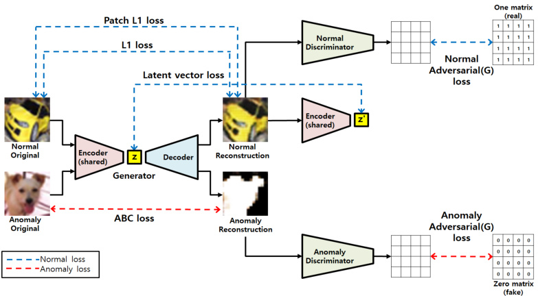
Fig. 1: Pipeline of the proposed approach for anomaly detection.
图 1: 所提出的异常检测方法流程。
Table 1: Imbalance problems and solutions of the proposed method
表 1: 所提方法的不平衡问题及解决方案
| 不平衡问题 | 解决方案 |
|---|---|
| 类别不平衡 | 基于k-means聚类的数据采样 (章节3.5) |
| 损失尺度不平衡 | 损失函数权重搜索 (章节3.4) |
| 判别器分布偏差 | 双判别器架构 (章节3.3) |
| 目标(缺陷)与图像的尺寸不平衡 | 基于重建的方法 |
Class imbalance
类别不平衡
Class imbalance is well known, and surface defects of metal cases such as scratch, stamped, and stain are very unlikely to happen in the production process, therefore resulting in outstanding class imbalance problems between normal and anomaly. Not only the number of normal and defective data is imbalanced, but also the frequency of occurrence differ among the types of defects such as scratch, stamped, and stain, so imbalance within each class exists in anomaly data. To resolve such class imbalance, data is partially sampled and used in training. Here, if the data is sampled randomly without considering its distribution, the entire data and the sampled data might not be balanced in their distribution. Therefore, in this paper,we use the method of dividing the entire data into several groups by k-means clustering, and then sample the same number of data within each group.
类别不平衡问题众所周知,金属外壳的表面缺陷(如划痕、压痕和污渍)在生产过程中极少发生,导致正常样本与异常样本之间存在显著的类别不平衡。不仅正常数据与缺陷数据数量失衡,划痕、压痕和污渍等各类缺陷的出现频率也存在差异,因此异常数据内部也存在类别不平衡。为解决此类不平衡问题,本研究采用部分采样数据进行训练。若随机采样而不考虑数据分布,整体数据与采样数据的分布可能仍不平衡。为此,本文采用k-means聚类将整体数据划分为若干组,然后在每组内抽取等量数据的采样方法。
Loss function scale imbalance
损失函数尺度不平衡
The proposed method uses the weighted sum of 6 types of loss functions to train the generator. The scale of the loss function used here is different, and even if the scale is the same, the effect on the learning is different. In addition, GAN contains a min-max problem that the generator and the disc rim in at or learn by competing against each other, making the learning difficult and unstable. The loss scales of the generator and the disc rim in at or should be sought at a similar rate to each other so that GAN is effectively trained. To handle such loss function scale imbalance problems, weights used in loss combination are explored by a grid search.
所提出的方法采用6种损失函数的加权和来训练生成器。此处使用的损失函数规模不同,即使规模相同,对学习的影响也有所差异。此外,GAN包含一个极小极大问题,即生成器与判别器通过相互竞争进行学习,这使得学习过程困难且不稳定。生成器与判别器的损失规模应以相近的速率进行调整,才能有效训练GAN。为处理此类损失函数规模不平衡问题,我们通过网格搜索探索了损失组合中使用的权重。
Disc rim in at or distribution al bias
判别器分布偏差
The loss will be used to update the generator differently for normal and anomaly data. When the reconstruction data is given to the disc rim in at or, the generator is trained to output 1 from normal data and 0 from anomaly data. Thus, when training from both normal and anomaly data, using a single disc rim in at or results in training the model to classify only normal images well. Separating discriminator for normal data and for anomaly data is necessary to solve this problem. This method only increases the parameters or computations of the model in the training phase, but not those in inference phase. As a result, there is no overall increase in memory usage or latency at the final inferences.
损失函数将分别用于更新生成器对正常数据和异常数据的处理。当重建数据输入判别器时,生成器的训练目标是使正常数据输出1、异常数据输出0。因此,在同时使用正常和异常数据训练时,单一判别器会导致模型仅擅长分类正常图像。为解决该问题,必须分别为正常数据和异常数据配置独立判别器。该方法仅在训练阶段增加模型参数量或计算量,推理阶段不会产生额外开销,因此最终推断时的内存占用和延迟不会整体增加。
Size imbalance between object(defect) and image
物体(缺陷)与图像之间的尺寸不平衡
Industrial defect data exhibits smaller size of defect compared to the size of the entire image. Objects in such data occupy very small portion of the image, making it closer to object detection rather than classification, so it is difficult to expect fair performance with classification methods. To solve this, we propose a method generating images to make the total reconstruction error bigger not affected by the size of the defect and the size of the entire image which contains the defect.
工业缺陷数据中,缺陷尺寸相对于整张图像往往较小。这类数据中的目标物体仅占据图像的极小部分,使其更接近目标检测任务而非分类任务,因此难以通过分类方法获得理想性能。为解决该问题,我们提出一种图像生成方法,通过增大整体重建误差来消除缺陷尺寸与含缺陷图像尺寸的影响。
3.3 Network Architecture
3.3 网络架构
The proposed model is a GAN-based network structure consisting of a generator and a disc rim in at or. The generator is in the form of an auto encoder to perform image to image translation. And a modified U-Net[39] structure is adopted, which has an effective delivery of features using a pyramid architecture. The disc rim in at or is a general CNN network, and two disc rim in at or s are used only in the training phase.
所提出的模型是一种基于GAN的网络结构,由生成器和判别器组成。生成器采用自编码器形式执行图像到图像的转换,并采用改进的U-Net[39]结构,该结构通过金字塔架构实现高效的特征传递。判别器为常规CNN网络,训练阶段仅使用两个判别器。
The generator is a symmetric network that consists of four 4 x 4 convolutions with stride 2 followed by four transposed convolutions. The total parameters of generator is composed of a sum of 0.38K, 2.08K, 8.26K. 32.9K, 32.83K, 16.42K, 4.11K, and 0.77K, that is 97.75K totally. The disc rim in at or is a general network that consists of three 4 x 4 convolutions with stride 2 followed by two 4 x 4 convolutions with stride 1. The total parameters of disc rim in at or is composed of a sum of 0.38K, 2.08K, 8.26K, 32.9K, and 32.77K, that is 76.39K.
生成器是一个对称网络,由四个步长为2的4x4卷积层和四个转置卷积层组成。生成器总参数量为0.38K、2.08K、8.26K、32.9K、32.83K、16.42K、4.11K和0.77K之和,总计97.75K。判别器是一个常规网络,由三个步长为2的4x4卷积层和两个步长为1的4x4卷积层组成。判别器总参数量为0.38K、2.08K、8.26K、32.9K和32.77K之和,总计76.39K。
3.4 Loss Function
3.4 损失函数
Total number of loss functions used in the proposed model is eight. Six losses for training of generator, one for normal disc rim in at or and another for anomaly disc rim in at or. The loss function for training of each disc rim in at or is adopted
所提模型共使用八个损失函数。其中六个用于生成器训练,一个用于正常判别器,另一个用于异常判别器。每个判别器的训练均采用相应损失函数。
from LSGAN [31] as shown in Eq. (1). It uses the a-b coding scheme for the disc rim in at or, where a and b are the labels for fake data and real data, respectively.
如式 (1) 所示,该方法借鉴了LSGAN [31] 的a-b编码方案,其中a和b分别代表伪造数据和真实数据的标签。
$$
\operatorname{min}{D}V_{\mathrm{LSGAN}}(D)=\left[\left(D(x)-b\right)^{2}\right]+\left[\left(D(G(x))-a\right)^{2}\right]
$$
$$
\operatorname{min}{D}V_{\mathrm{LSGAN}}(D)=\left[\left(D(x)-b\right)^{2}\right]+\left[\left(D(G(x))-a\right)^{2}\right]
$$
Six kinds of loss functions, as shown in from Eq. (2) to (8) are employed to train the generator. Among them, four losses are for normal images. First, L1 reconstruction error of generator for normal image is provided as shown in Eq. (2). It penalizes by measuring the L1 distance between the original $x$ and the generated images ( ${\hat{x}}=G(x)$ ) as defined in [1]:
采用六种损失函数(如式(2)至(8)所示)训练生成器。其中四种损失函数针对正常图像:首先计算正常图像的生成器L1重建误差(如式(2)所示),通过测量原始图像$x$与生成图像${\hat{x}}=G(x)$之间的L1距离进行惩罚,定义见[1]:
$$
\mathcal{L}{\mathrm{recon}}=|x-G(x)|_{1}
$$
$$
\mathcal{L}{\mathrm{recon}}=|x-G(x)|_{1}
$$
Second, the patch loss is newly proposed in this paper as shown in Eq. (3). Divide a normal image and a generated image separately into M patches and select the average of the biggest n reconstruction errors among all the patches.
其次,本文新提出的补丁损失如式(3)所示。将正常图像和生成图像分别划分为M个补丁,并选取所有补丁中前n个最大重建误差的平均值。
$$
\mathcal{L}{\mathrm{patch}}=f_{a v g}(n)(\left|\left|x_{p a t c h(i)}-G(x_{p a t c h(i)})\right|\right|_{1}),i=1,2,...,m
$$
$$
\mathcal{L}{\mathrm{patch}}=f_{a v g}(n)(\left|\left|x_{p a t c h(i)}-G(x_{p a t c h(i)})\right|\right|_{1}),i=1,2,...,m
$$
Third, latent vector loss [1] is calculated as the difference between latent vectors of generator for normal image and latent vectors of cascaded encoder for reconstruction image as shown in Eq. (4)
第三,潜在向量损失 [1] 的计算方式如公式 (4) 所示,即正常图像的生成器潜在向量与重建图像的级联编码器潜在向量之间的差值。
$$
\mathcal{L}{\mathrm{enc}}=|G_{E}(x)-G_{E}(G(x))|_{1}
$$
$$
\mathcal{L}{\mathrm{enc}}=|G_{E}(x)-G_{E}(G(x))|_{1}
$$
Eq. (5) defines the proposed adversarial loss for the generator update use in LSGAN[31], where $y$ denotes the value that G wants D to believe for fake data.
式 (5) 定义了 LSGAN [31] 中用于生成器更新的对抗损失,其中 $y$ 表示生成器希望判别器对伪造数据所置信的值。
$$
{min}{G}V_{LSGAN}(G)=[(D(G(x))-y)^{2}]
$$
Fourth, the adversarial loss used to update the generator is as shown in Eq. (6). The loss function intends to output a real label of 1 when a reconstruction image (fake) is into the disc rim in at or.
第四,用于更新生成器的对抗损失如式(6)所示。该损失函数旨在当重建图像(伪造)输入判别器时输出真实标签1。
$$
{min}{G}V_{LSGAN}(G)=[(D(G(x))-1)^{2}]
$$
Two remaining losses for anomaly images are as follows. One is anomaly adversarial loss for updating generator and the other is ABC [51] loss. Unlike a general adversarial loss of Eq (6), anomaly reconstruction image should be generated differently from real one to classify anomaly easily, the anomaly adversarial loss newly adopted in our work is as shown in Eq. (7).
异常图像的两个剩余损失如下:一是用于更新生成器的异常对抗损失,另一个是ABC [51]损失。与式(6)的一般对抗损失不同,异常重建图像应生成得与真实图像不同以便更容易分类异常,本文新采用的异常对抗损失如式(7)所示。
$$
{min}{G}V_{LSGAN}(G)=[(D(G(x))-0)^{2}]
$$
ABC loss as shown Eq. (8) is used here to maximize L1 reconstruction error $\mathcal{L}_{\boldsymbol{\theta}}(\cdot)$ for anomaly data. Because the difference between the reconstruction errors
此处采用式(8)所示的ABC损失函数,通过最大化异常数据的L1重建误差$\mathcal{L}_{\boldsymbol{\theta}}(\cdot)$来实现。由于重建误差之间的差异
for normal and anomaly data is large, the equation is modified by adding the exponetial and log function to solve the scale imbalance.
对于正常和异常数据差异较大的情况,通过引入指数函数和对数函数来修正方程,以解决尺度不平衡问题。
$$
\mathcal{L}{\mathrm{ABC}}=-\mathrm{log}(1-e^{-\mathcal{L}{\theta}(x_{i})})
$$
$$
\mathcal{L}{\mathrm{ABC}}=-\mathrm{log}(1-e^{-\mathcal{L}{\theta}(x_{i})})
$$
Total loss function consists of weighted sum of each loss. All losses for normal images are grouped together and same as for anomaly images. Those two group of losses are applied to update the weights of learning process randomly. The scale imbalances exist among the loss functions. Although the scale could be adjusted in same range, the effect might be different, so we explore the weight of each loss using the grid search. Because ABC loss can have the largest scale, the weighted sum of normal data is set more than twice as large as the weighted sum of anomaly data. In order to avoid huge and unnecessary search space, each weight of the loss functions is limited from 0.5∼1.5 range. Then the grid search is executed the each weight adjusting by 0.5. Total possible cases for the grid search is 314. The final explored weights of loss function are shown in Table 2.
总损失函数由各损失项的加权和构成。正常图像的所有损失归为一组,异常图像同理。这两组损失被随机用于更新学习过程的权重。各损失函数间存在尺度不平衡问题。虽然可将尺度调整至相同范围,但效果可能不同,因此我们采用网格搜索探索各损失权重。由于ABC损失可能具有最大尺度,正常数据的加权和被设定为异常数据的两倍以上。为避免庞大且不必要的搜索空间,各损失函数的权重限制在0.5∼1.5范围内,并以0.5为步长进行网格搜索,总搜索可能性为314种。最终探索的损失函数权重如表2所示。
Table 2: Weight combination of loss functions obtained by Grid search
表 2: 通过网格搜索获得的损失函数权重组合
| 常规重建L1损失 | ABC损失 | 常规对抗损失 | 常规重建分块L1损失 | 常规潜向量损失 | 异常对抗损失 |
|---|---|---|---|---|---|
| 1.5 | 0.5 | 0.5 | 1.5 | 0.5 | 1.0 |
3.5 Data Sampling
3.5 数据采样
As mentioned in section 3.2, the experimental datasets include imbalance problems. For benchmark datasets such as MNIST, Fashion-MNIST, CIFAR-10, and CIFAR-100, have a class imbalance problems presenting imbalance of data sampling. The real-world dataset, surface defects of smartphone case is not only the number of normal and defective data are imbalanced, but also the frequency of occurrences differs among the types of defects. Also the size of image and object (defect) is imbalanced too. To solve those imbalance problem, k-means clustering-based data sampling is performed to make balanced distribution of data. In learning stage for benchmark datasets, all data is used for normal case. In case of anomaly, the same number is sampled for each class so that the total number of data is similar to normal. At this time, k-means clustering is performed on each class, and data is sampled from each cluster in a distribution similar to the entire dataset. For anomaly case of defect dataset, data is sampled using the same method as the benchmark, and a number of normal data is sampled, equal to the number of data combined with the three kinds of defects - scratch, stamped and stain. Detail number of data is described in section 4.1
如第3.2节所述,实验数据集存在不平衡问题。对于MNIST、Fashion-MNIST、CIFAR-10和CIFAR-100等基准数据集,存在数据采样不平衡的类别不平衡问题。真实世界数据集智能手机外壳表面缺陷不仅正常与缺陷数据数量不平衡,各类缺陷的出现频率也存在差异,且图像与缺陷对象的尺寸也不均衡。为解决这些不平衡问题,采用基于k-means聚类的数据采样方法实现数据均衡分布。在基准数据集的学习阶段,正常情况使用全部数据;异常情况则对每个类别采样相同数量,使总数据量与正常情况相近。此时对每个类别执行k-means聚类,并按与整体数据集相似的分布从各簇中采样数据。对于缺陷数据集的异常情况,采用与基准数据集相同的采样方法,并采样与划痕、压痕、污渍三类缺陷数据总数相等的正常数据量。具体数据数量详见第4.1节
4 Experiments
4 实验
In this section, we perform substantial experiments to validate the proposed method for anomaly detection. We first evaluate our method on commonly used benchmark datasets - MNIST, Fashion-MNIST, CIFAR-10, and CIFAR100. Next, we conduct experiments on real-world anomaly detection dataset - smartphone case defect dataset. Then we present the respective effects of different designs of loss functions through ablation study.
在本节中,我们进行了大量实验以验证所提出的异常检测方法。首先在常用基准数据集(MNIST、Fashion-MNIST、CIFAR-10和CIFAR100)上评估方法性能,随后在真实场景的智能手机外壳缺陷数据集上进行测试。最后通过消融实验展示不同损失函数设计的具体影响。
4.1 Datasets
4.1 数据集
Datasets used in the experiments include of four standard image datasets: MNIST [27], Fashion-MNIST[47], CIFAR-10[24], and CIFAR-100[24]. Additional y smartphone case defect data is added to evaluate the performance in real-world environments.
实验中使用的数据集包括四个标准图像数据集:MNIST [27]、Fashion-MNIST [47]、CIFAR-10 [24] 和 CIFAR-100 [24]。此外还添加了智能手机外壳缺陷数据以评估现实环境中的性能。
For MNIST, Fashion-MNIST, CIFAR-10 data set, each class is defined as normal and the rest of nine classes are defined as anomaly. Total 10 experiments are performed by defining each 10 class once as normal. With CIFAR-100 dataset, one class is defined as normal and the remaining 19 classes are defined as anomaly among 20 super classes. Each superclass is defined as normal one by one, so in total 20 experiments were conducted. Also, in order to resolve imbalance in the number of normal data and anomaly data, and in distribution of sampled data, the method proposed in 3.5 is applied when sampling training data. 6000 normal and anomaly data images were used for training MNIST and Fashion-MNIST, and 5000 were used for CIFAR-10. Additionally, for MNIST and Fashion-MNIST, the images were resized into 32x32 so that the size of the feature can be the same when concatenating them in the network structure.
对于MNIST、Fashion-MNIST和CIFAR-10数据集,每个类别被定义为正常类,其余九个类别被定义为异常类。通过依次将10个类别中的每一个定义为正常类,共进行了10次实验。在使用CIFAR-100数据集时,20个超类中一个类别被定义为正常类,其余19个类别被定义为异常类。每个超类依次被定义为正常类,因此总共进行了20次实验。此外,为解决正常数据和异常数据数量不平衡以及采样数据分布不均的问题,在采样训练数据时应用了3.5节提出的方法。训练MNIST和Fashion-MNIST时使用了6000张正常和异常数据图像,CIFAR-10使用了5000张。另外,对于MNIST和Fashion-MNIST,图像被调整为32x32大小,以便在网络结构中拼接时特征尺寸保持一致。
Smartphone case defect dataset consists of normal, scratch, stamped and stain classes. And there are two main types of data set. The first dataset contains patch images that are cropped into 100x100 from their original size of 2192x1000 . The defective class is sampled in the same number as the class with the least number of data among defects by deploying the method from section 3.5, and the normal data is sampled in a similar number to that of the detective data. 900 images of normal data and 906 images of anomaly data were used for training, and 600 images of normal data and 150 images of anomaly data were used for testing. In the experiments, images were resized from 100x100 to 128x128. The second dataset consists of patch images cropped into 548x500. The same method of sampling as the 100x100 patch images is used. 1800 images of normal data and 1814 images of anomaly data are used for training, and 2045 images of normal data and 453 images of normal data are used for testing.
智能手机外壳缺陷数据集包含正常、划痕、压印和污渍四种类别。数据集主要分为两种类型:第一种数据集包含从原始尺寸2192x1000裁剪为100x100的局部图像。通过采用3.5节所述方法,缺陷类别采样数量与缺陷中最少数据的类别保持一致,正常数据采样数量与缺陷数据相近。训练集使用900张正常图像和906张异常图像,测试集使用600张正常图像和150张异常图像。实验中图像尺寸从100x100调整为128x128。第二种数据集包含裁剪为548x500的局部图像,采样方法与100x100局部图像相同。训练集使用1800张正常图像和1814张异常图像,测试集使用2045张正常图像和453张异常图像。
4.2 Experimental Setups
4.2 实验设置
Experimentation is performed using Intel Core i7-9700K $@$ 3.60GHz and NVIDIA geforce GTX 1080ti with Tensorflow 1.14 deep learning framework. For augmentation on MNIST, the method of randomly cropping 0∼2 pixels from the boundary and resizing again was used, while for Fashion-MNIST, images were vertically and horizontally flipped, randomly cropped 0∼2 pixels from their boundary, and resized again. Then, the images were rotated 90, 180, or 270 degrees. For CIFAR-10 and CIFAR-100, on top of the augmentation method utilized for Fashion-MNIST, hue, saturation, brightness, and contrast are varied as additional augmentation. For defective dataset, vertical flipping and horizontal flipping are used along with rotation of 90, 180, or 270 degrees.
实验采用Intel Core i7-9700K $@$ 3.60GHz处理器和NVIDIA GeForce GTX 1080ti显卡,搭配TensorFlow 1.14深度学习框架进行。对于MNIST数据集的数据增强,采用了从边界随机裁剪0∼2像素并重新调整大小的方法;而Fashion-MNIST则进行了垂直和水平翻转、从边界随机裁剪0∼2像素后重新调整大小,并旋转90、180或270度。针对CIFAR-10和CIFAR-100数据集,在Fashion-MNIST所用增强方法基础上,额外调整了色调、饱和度、亮度及对比度作为补充增强手段。缺陷数据集的处理则采用了垂直翻转、水平翻转以及90、180或270度的旋转操作。
Hyper parameters and details on augmentation are as follows Table 3.
超参数和数据增强细节如下表3。
Table 3: Hyper parameters used for model training
表 3: 模型训练使用的超参数
| 超参数 | 块重建误差参数:损失 (Eq. 3) | ||||||
|---|---|---|---|---|---|---|---|
| 训练轮数 | 批次大小 | 初始学习率 | 学习率衰减轮数 | 学习率衰减因子 | 块大小 | 步长 | 选取块数量 |
| 300 | 1 | 0.0001 | 50 | 0.5 | 16 | 8 | 3 |
4.3 Benchmarks Results
4.3 基准测试结果
In order to evaluate the performance of our proposed method, we conducted experiments on MNIST, Fashion-MNIST, CIFAR-10 and CIFAR-100. For estimating recognition rates of the trained model, AUROC(Area Under the Receiver Operating Characteristic) is used. Table 5 contains State-Of-The-Art studies and their recognition rates, and Figure 2 compares recognition rates, model parameters, and FPS on CIFAR-10 among the representative studies.
为了评估我们提出的方法性能,我们在MNIST、Fashion-MNIST、CIFAR-10和CIFAR-100数据集上进行了实验。使用AUROC(Area Under the Receiver Operating Characteristic)指标来评估训练模型的识别率。表5包含了当前最先进的研究及其识别率,图2比较了代表性研究在CIFAR-10上的识别率、模型参数和FPS。
According to Table 5, for the MNIST, the paper with highest performance among previous studies is ARNet, which presented average AUROC value of 98.3 for 10 classes, however our method obtains average AUROC of 99.7 with the proposed method. Also, ARNet have standard deviation of 1.78 while ours shows 0.16, therefore significantly reducing deviations among classes. For the Fashion-MNIST, ARNet previously performs the best with average AUROC of 93.9 and standard deviation of 4.7, but our method accomplishes much better results of average AUROC of 98.6 and standard deviation 1.20. For the CIFAR10, the average AUROC ARNet, so far as the best, with is 86.6 with standard deviation 5.35, but our method achieves quite better result of average AUROC of 90.6 with standard deviation 3.14. Lastly, for CIFAR-100, compared to the results from ARNet, which are average AUROC of 78.8 and standard deviation 8.82, the proposed method shows outstanding improvement of average AUROC 87.4 and standard deviation 4.80. In summary, four different datasets were used for evaluating the performance, and we achieve highly improved results from the previous State-Of-The-Arts studies in terms of recognition rate and learning stability on all the tested datasets.
根据表5,在MNIST数据集上,先前研究中表现最佳的论文是ARNet,其对10个类别的平均AUROC值为98.3,而我们的方法通过所提方案实现了99.7的平均AUROC。此外,ARNet的标准差为1.78,而我们的方法仅为0.16,显著降低了类别间的偏差。在Fashion-MNIST数据集上,ARNet此前以93.9的平均AUROC和4.7的标准差保持最优,但我们的方法取得了98.6的平均AUROC和1.20标准差的更优结果。对于CIFAR10数据集,当前最佳结果ARNet的平均AUROC为86.6(标准差5.35),而我们的方法实现了90.6的平均AUROC(标准差3.14)的显著提升。最后在CIFAR-100数据集上,相较于ARNet的78.8平均AUROC(标准差8.82),所提方法展现出87.4平均AUROC(标准差4.80)的卓越改进。总体而言,我们在四个不同测试集上的实验表明,该方法在所有数据集的识别率和学习稳定性方面均较现有最优研究取得了显著提升。
Figure 2 shows a graph that compares the performance of State-Of-TheArts researches regarding for average AUROC, FPS, and the number of model parameters used in inference. FPS is calculated as averaging total 10 estimations of processing time for 10,000 CIFAR-10 images. In the graph, the x-axis stands for FPS, i.e. how many images are inferred per second, and the y-axis represents AUROC( $%$ ), the recognition rate. The area of the circle of each method indicates the number of model parameters used in inference. The graph shows that our method has AUROC of $90.6%$ , which is 4% higher than that of ARNet, $86.6%$ , known to be the highest in the field. Among the papers mentioned, GeoTrans has the least number of model parameters, 1,216K. However, the model proposed in this paper require 98K parameters, which only 8% of those of GeoTrans therefore resulting in huge reduction. Finally in terms of FPS, ARNet was known to be the fastest with 270FPS, the proposed method was able to process with 532FPS, almost twice as fast.
图 2: 展示了当前最优研究的平均AUROC、FPS及推理所用模型参数量对比图。FPS通过10次处理10,000张CIFAR-10图像的平均耗时计算得出。图中横轴代表FPS (每秒推理图像数) ,纵轴表示AUROC( $%$ )识别率。各方法圆点面积对应推理所用模型参数量。数据显示,本方法AUROC达 $90.6%$ ,较领域最高记录ARNet的 $86.6%$ 提升4%。在提及的论文中,GeoTrans参数量最低(1,216K) ,而本文提出的模型仅需98K参数,为GeoTrans的8%,实现大幅精简。FPS方面,ARNet以270FPS保持最快记录,本方法则达到532FPS,速度提升近一倍。

Fig. 2: Comparison of AUROC, FPS, and model parameters for CIFAR10 dataset.
图 2: CIFAR10数据集的AUROC、FPS和模型参数对比。
Table 4: AUROC results for defect dataset ( $%$ )
表 4: 缺陷数据集的AUROC结果 ( $%$ )
| 数据集 | 训练集 | 测试集 |
|---|---|---|
| 100x1 100 patch缺陷 | 99.73 | 99.23 |
| 548x500 patch缺陷 | 99.74 | 98.84 |
4.4 Defect Dataset Results
4.4 缺陷数据集结果
Table 4 shows the experiment results with smartphone detective dataset. Testing for 100x100 patch images, the performance is absolutely high with AUROC( $%$ ) of 99.23. The bigger size of image data with 548x500 patch, much more difficult than of 100x100 patch data, is tested and shows very similar results of 98.84 still. Therefore, the superiority of our method is proved even in real-world smartphone detective dataset.
表 4 展示了智能手机检测数据集的实验结果。测试 100x100 图像块时性能极高,AUROC( $%$ )达到 99.23。针对更具挑战性的 548x500 大尺寸图像块(相比 100x100 数据难度显著提升)进行测试,仍保持 98.84 的相近结果。这证明我们的方法在真实智能手机检测数据集上仍具优越性。
Table 5: Comparison with the state-of-the-art literature in AUROC(%) for benchmark datasets
表 5: 基准数据集AUROC(%)与现有文献对比
| 数据集 | 方法 | 0 | 1 | 2 | 3 | 4 | 5 | 6 | 7 | 8 | 9 | avg | SD |
|---|---|---|---|---|---|---|---|---|---|---|---|---|---|
| MNIST | AE VAE[21] | 98.8 | 99.3 | 91.7 | 88.5 | 86.2 | 92.1 | 99.9 | 81.5 | 81.4 | 87.9 | 81.19 | 5.90 |
| AnoGAN[43] | 85.8 | 95.4 | 94.0 | 82.3 | 96.5 | 91.9 | 94.3 | 88.6 | 78.0 | 92.0 | 87.7 | 7.05 | |
| ADGAN[10] | 97.2 | 99.6 | 85.1 | 90.6 | 94.5 | 94.9 | 97.1 | 93.9 | 79.7 | 95.4 | 92.8 | 4.15 | |
| GANomaly[1] | 98.2 | 91.6 | 99.4 | 99.0 | 99.1 | 99.8 | 99.9 | 94.2 | 96.3 | 97.5 | 97.5 | 6.12 | |
| OCGAN[35] | 98.6 | 99.9 | 99.0 | 99.1 | 98.1 | 98.1 | 99.6 | 99.9 | 96.3 | 97.2 | 98.0 | 2.50 | |
| GeoTrans[13] | 99.9 | 99.9 | 99.7 | 99.8 | 99.7 | 99.8 | 99.7 | 99.7 | 99.5 | 99.4 | 99.7 | 0.16 | |
| ARNet[18] | 99.5 | 99.6 | 98.2 | 98.6 | 98.1 | 99.5 | 95.9 | 99.4 | 97.6 | 99.6 | 98.6 | 1.20 | |
| OURS | 57.1 | 54.9 | 59.9 | 62.3 | 63.9 | 57.0 | 68.1 | 53.8 | 64.4 | 48.6 | 59.0 | 5.84 | |
| Fashion-MNIST | AE | 41.4 | 57.1 | 56.0 | 48.3 | 61.9 | 50.1 | 73.3 | 60.5 | 53.8 | 51.2 | 52.2 | 5.95 |
| VAE[21] | 61.0 | 56.5 | 64.8 | 52.8 | 67.0 | 59.2 | 62.5 | 57.6 | 72.3 | 58.2 | 61.2 | 5.68 | |
| DAGMM[53] | 63.2 | 52.9 | 68.4 | 53.3 | 73.9 | 63.6 | 60.9 | 93.5 | 60.8 | 59.1 | 58.0 | 9.10 | |
| DSEBM[55] | 58.2 | 72.4 | 62.2 | 60.6 | 60.7 | 65.9 | 61.1 | 63.0 | 88.6 | 56.0 | 76.0 | 13.08 | |
| AnoGAN[43] | 74.7 | 95.7 | 78.1 | 75.7 | 53.1 | 64.0 | 62.0 | 72.3 | 57.5 | 82.0 | 65.6 | 9.52 | |
| ADGAN[10] | 78.5 | 89.8 | 86.1 | 77.4 | 90.5 | 84.5 | 89.2 | 92.9 | 92.0 | 85.5 | 86.6 | 8.52 | |
| GANomaly[1] | 92.6 | 93.6 | 86.9 | 85.4 | 89.5 | 87.8 | 93.5 | 91.0 | 94.6 | 91.7 | 90.6 | 3.14 | |
| GeoTrans[13] | 74.7 | 68.5 | 74.0 | 81.0 | 78.4 | 59.1 | 57.9 | 51.9 | 36.0 | 46.5 | 46.6 | 5.35 | |
| ARNet[18] | 77.5 | 70.0 | 62.4 | 76.2 | 77.7 | 64.0 | 86.9 | 65.6 | 82.7 | 90.2 | 85.9 | 8.11 | |
| OURS | 85.5 | 86.1 | 94.4 | 87.3 | 91.7 | 85.1 | 89.9 | 88.3 | 83.8 | 92.4 | 94.2 | 6.55 | |
| CIFAR-10 | AE | 62.1 | 46.4 | 62.7 | 59.6 | 42.7 | 66.8 | 49.8 | 45.4 | 57.2 | 52.6 | 44.0 | 9.36 |
| DAGMM[53] | 48.1 | 48.8 | 54.4 | 56.8 | 63.1 | 36.4 | 52.4 | 73.0 | 57.7 | 41.5 | 50.3 | 8.11 | |
| DSEBM[55] | 55.5 | 52.4 | 50.5 | 58.8 | 62.1 | 46.4 | 62.7 | 59.6 | 42.7 | 66.8 | 49.8 | 6.55 | |
| ADGAN[10] | 45.4 | 57.2 | 52.6 | 44.0 | 48.1 | 48.8 | 54.4 | 56.8 | 63.1 | 36.4 | 52.4 | 9.36 | |
| GANomaly[1] | 73.0 | 57.7 | 41.5 | 50.3 | 55.5 | 52.4 | 50.5 | 58.8 | 62.1 | 46.4 | 62.7 | 8.11 | |
| GeoTrans[13] | 59.6 | 42.7 | 66.8 | 49.8 | 45.4 | 57.2 | 52.6 | 44.0 | 48.1 | 48.8 | 54.4 | 6.55 | |
| ARNet[18] | 56.8 | 63.1 | 36.4 | 52.4 | 73.0 | 57.7 | 41.5 | 50.3 | 55.5 | 52.4 | 50.5 | 9.36 | |
| OURS | 58.8 | 62.1 | 46.4 | 62.7 | 59.6 | 42.7 | 66.8 | 49.8 | 45.4 | 57.2 | 52.6 | 8.11 |
4.5 Ablation Studies
4.5 消融实验
To understand how each loss affect GAN-based anomaly learning, we defined CIFAR-10 bird class as normal and the rest of the classes as anomaly, and conducted an ablation study. The network structure and learning parameters are the same as the experiments with the benchmarks, and training data is also sampled based on k-means clustering to 5000 normal and 5000 anomaly images. All of the given testing data from the dataset is used for testing. The results shows that the performance improves as each loss gets added to the basic auto encoder. In the Table 6, No.2(only ABC added) and No.7(all losses added) don’t show much difference in AUROC, $85.44%$ and $86.76%$ . However, from Figure 3 it can be found that reconstructed images exhibits significant difference. It visualizes the result of experiment No.2 and No.7 with normal data. In the case of ABC, the normal images could not be reconstructed similarly, so the center was made 0 due to loss from anomaly. On the other hand, experiment No.7 which exploited combination of the proposed losses reconstructed the image similarly to the original. The average error regarding reconstruction error map also shows difference of 2∼3 times.
为了解每种损失对基于GAN的异常学习的影响,我们将CIFAR-10鸟类类别定义为正常样本,其余类别作为异常样本进行消融实验。网络结构和学习参数与基准测试实验相同,训练数据同样通过k-means聚类采样得到5000张正常图像和5000张异常图像。测试阶段使用数据集中全部测试数据。结果表明,随着各项损失函数逐步加入基础自编码器,模型性能持续提升。表6中,实验2(仅添加ABC损失)与实验7(添加全部损失)的AUROC指标差异不大(85.44% vs 86.76%)。但如图3所示,两者的重建图像存在显著差异。该图可视化展示了实验2和实验7在正常数据上的重建效果:仅使用ABC损失时,正常图像无法被准确重建,由于异常损失的影响导致中心区域归零;而采用全部损失组合的实验7则能实现接近原始图像的重建效果。重建误差图的平均误差值也显示出2∼3倍的差异。
Table 6: Ablation study experiment results to confirm the impact of losses used in generator update $'A U R O C(%)\Big)$ )
表 6: 用于确认生成器更新中使用损失影响的消融研究实验结果 $'A U R O C(%)\Big)$
| No. | Auto Encoder | ABC | Normal | Generator Anomaly | Normal patch | Normal latent | AUROC |
|---|---|---|---|---|---|---|---|
| 1 | 64.68 | ||||||
| 2 | 85.44 | ||||||
| 3 | √ | √ | 65.74 | ||||
| 4 | √ | 65.93 | |||||
| 5 | 64.87 | ||||||
| 6 | √ | √ | 64.89 | ||||
| 7 | √ | √ | √ | √ | √ | 86.76 |

Fig. 3: Visualized results for No.2 and No.7 experiments in ablation study
图 3: 消融研究中2号与7号实验的可视化结果

Fig. 4: Visualization of experimental results on the Benchmark dataset & defect data (Original, reconstruction, reconstruction error map order from the left of each image)
图 4: Benchmark数据集和缺陷数据的实验结果可视化 (每张图像从左至右依次为: 原始图像、重建图像、重建误差图)
5 Conclusion
5 结论
We proposed a novel GAN-based anomaly detection model by using a new framework, newly defined loss functions, and optimizing their combinations. The discri minato rs for normal and anomaly are structurally separated to improve the learning that has been biased toward normal data. Also, a new definition of patch loss and anomaly adversarial loss, which are effective for fault detection was introduced and combined with the major losses proposed from previous studies to perform joint learning. In order to systemize the proportion of each loss in the combination, the weight of each loss was explored using the grid search. The main results of our experiments successfully demonstrated that the proposed method much further improves the AUROC for CIFAR-10 data compared to the results of State-Of-The-Art including GANomaly[1], GeoTrans[13] and ARNet[18]. Especially, we applied our method to real-world data set with surface defects of smartphone case and validated outstanding superiority of anomaly detection of the defects. In the future, we will try to extend our approach to a hierarchical anomaly detection scheme from pixel level to video level.
我们提出了一种基于GAN(生成对抗网络)的新型异常检测模型,该模型采用全新框架、新定义的损失函数并优化了它们的组合。通过结构分离正常与异常的判别器,改善了原本偏向正常数据的学习模式。同时引入对故障检测有效的补丁损失和异常对抗损失新定义,将其与先前研究提出的主要损失函数相结合进行联合学习。为系统化各损失函数的组合比例,我们采用网格搜索法探索了各损失权重。实验主要成果表明,相比GANomaly[1]、GeoTrans[13]和ARNet[18]等前沿方法,所提方案显著提升了CIFAR-10数据的AUROC指标。特别地,我们将该方法应用于智能手机外壳表面缺陷的真实数据集,验证了其在缺陷异常检测方面的卓越优势。未来将尝试将该方法扩展到从像素级到视频级的分层异常检测方案。