Input Perturbation Reduces Exposure Bias in Diffusion Models
Abstract
摘要
Denoising Diffusion Probabilistic Models have shown an impressive generation quality although their long sampling chain leads to high computational costs. In this paper, we observe that a long sampling chain also leads to an error accumulation phenomenon, which is similar to the exposure bias problem in auto regressive text generation. Specifically, we note that there is a discrepancy between training and testing, since the former is conditioned on the ground truth samples, while the latter is conditioned on the previously generated results. To alleviate this problem, we propose a very simple but effective training regu lari z ation, consisting in perturbing the ground truth samples to simulate the inference time prediction errors. We empirically show that, without affecting the recall and precision, the proposed input perturbation leads to a significant improvement in the sample quality while reducing both the training and the inference times. For instance, on CelebA $64\times64$ , we achieve a new state-of-theart FID score of 1.27, while saving $37.5%$ of the training time. The code is available at https: //github.com/forever208/DDPM-IP.
去噪扩散概率模型(Denoising Diffusion Probabilistic Models)虽然采样链较长导致计算成本较高,但其生成质量令人印象深刻。本文发现长采样链还会导致误差累积现象,这与自回归文本生成中的曝光偏差问题类似。具体而言,我们注意到训练与测试之间存在差异:前者以真实样本为条件,而后者则以先前生成的结果为条件。为缓解此问题,我们提出了一种简单有效的训练正则化方法,即通过扰动真实样本来模拟推理时的预测误差。实验表明,在不影响召回率和精确度的情况下,所提出的输入扰动方法显著提高了样本质量,同时减少了训练和推理时间。例如在CelebA $64\times64$ 数据集上,我们以节省 $37.5%$ 训练时间的代价,取得了1.27的最新FID分数。代码已开源:https://github.com/forever208/DDPM-IP。
1. Introduction
1. 引言
Denoising Diffusion Probabilistic Models (DDPMs) (SohlDickstein et al., 2015; Ho et al., 2020) are a new generative paradigm which is attracting a growing interest due to its very high-quality sample generation capabilities (Dhariwal & Nichol, 2021; Nichol et al., 2022; Ramesh et al., 2022). Differently from most existing generative methods which synthesize a new sample in a single step, DDPMs resemble the Langevin dynamics (Welling & Teh, 2011) and the generation process is based on a sequence of denoising steps, in which a synthetic sample is created starting from pure noise and auto regressive ly reducing the noise component. In more detail, during training, a real sample $\pmb{x}{0}$ is progressively destroyed in $T$ steps adding Gaussian noise (forward process). The sequence ${\pmb x}{0},...,{\pmb x}{t},...,{\pmb x}{T}$ so obtained, is used to train a deep denoising auto encoder $(\mu(\cdot))$ to invert the forward process: $\hat{\mathbf{\pmbx}}{t-1}=\mu(\mathbf{\pmbx}{t},t)$ . At inference time, the generation process is auto regressive because it depends on the previously generated samples: $\hat{\mathbf{x}}{t-1}=\mu(\hat{\mathbf{x}}_{t},t)$ (Sec. 3).
去噪扩散概率模型 (DDPMs) (SohlDickstein et al., 2015; Ho et al., 2020) 是一种新兴的生成范式,因其卓越的样本生成质量 (Dhariwal & Nichol, 2021; Nichol et al., 2022; Ramesh et al., 2022) 而受到广泛关注。与大多数单步生成样本的传统方法不同,DDPMs 采用类似朗之万动力学 (Welling & Teh, 2011) 的多步去噪策略:从纯噪声出发,通过自回归方式逐步降噪来合成样本。具体而言,在训练阶段,真实样本 $\pmb{x}{0}$ 会通过 $T$ 步高斯噪声添加被逐步破坏(前向过程)。由此获得的序列 ${\pmb x}{0},...,{\pmb x}{t},...,{\pmb x}{T}$ 用于训练深度去噪自编码器 $(\mu(\cdot))$ 以逆转前向过程:$\hat{\mathbf{\pmbx}}{t-1}=\mu(\mathbf{\pmbx}{t},t)$。在推理阶段,生成过程具有自回归特性,因为每一步生成都依赖于前序结果:$\hat{\mathbf{x}}{t-1}=\mu(\hat{\mathbf{x}}_{t},t)$(第3节)。
Despite the large success of DDPMs in different generative fields (Sec. 2), one of the main drawbacks of these models is their very long computational time, which depends on the large number of steps $T$ required at both the training and the inference stage. As recently emphasised in (Xiao et al., 2022), the fundamental reason why $T$ needs to be large is that each denoising step is assumed to be Gaussian, and this assumption holds only for small step sizes. Conversely, with larger step sizes, the prediction network $(\mu(\cdot))$ needs to solve a harder problem and it becomes progressively less accurate (Xiao et al., 2022). However, in this paper, we observe that there is a second phenomenon, related to the sampling chain, but partially in contrast with the first, which is the accumulation of these errors over the $T$ inference sampling steps. This is basically due to the discrepancy between the training and the inference stage, in which the latter generates a sequence of samples based on the results of the previous steps, hence possibly accumulating errors. In fact, at training time, $\mu(\cdot)$ is trained with a ground truth pair $({\pmb x}{t},{\pmb x}{t-1})$ and, given $\pmb{x}{t}$ , it learns to reconstruct $\pmb{x}{t-1}$ $(\mu(\pmb{x}{t},t))$ . However, at inference time, $\mu(\cdot)$ has no access to the “real” $\pmb{x}{t}$ , and its prediction depends on the previously generated $\hat{\pmb x}{t}$ $(\mu(\hat{\pmb x}{t},t))$ . This input mismatch between $\mu(\pmb{x}{t},t)$ , used during training, and $\mu(\hat{\mathbf{\boldsymbol{x}}}_{t},t)$ , used during testing, is similar to the exposure bias problem (Ranzato et al., 2016; Schmidt, 2019) shared by other auto regressive generative methods. For example, Rennie et al. (2017) argue that training a network to maximize the likelihood of the next ground-truth word given the previous ground-truth word (called “Teacher-Forcing” (Bengio et al., 2015)) results in error accumulation at inference time, since the model has never been exposed to its own predictions.
尽管 DDPM (Denoising Diffusion Probabilistic Models) 在不同生成领域取得了巨大成功 (第 2 节),但这些模型的主要缺点之一是计算时间非常长,这取决于训练和推理阶段所需的大量步骤 $T$。正如 (Xiao et al., 2022) 最近强调的那样,$T$ 需要很大的根本原因是每个去噪步骤都被假设为高斯分布,而这一假设仅适用于较小的步长。相反,步长较大时,预测网络 $(\mu(\cdot))$ 需要解决更困难的问题,并且其准确性会逐渐降低 (Xiao et al., 2022)。然而,在本文中,我们观察到第二种现象,它与采样链有关,但与第一种现象部分相反,即这些误差在 $T$ 个推理采样步骤中的累积。这基本上是由于训练和推理阶段之间的差异,后者基于前一步的结果生成一系列样本,因此可能累积误差。事实上,在训练时,$\mu(\cdot)$ 是用真实值对 $({\pmb x}{t},{\pmb x}{t-1})$ 训练的,给定 $\pmb{x}{t}$,它学会重建 $\pmb{x}{t-1}$ $(\mu(\pmb{x}{t},t))$。然而,在推理时,$\mu(\cdot)$ 无法访问“真实”的 $\pmb{x}{t}$,其预测依赖于之前生成的 $\hat{\pmb x}{t}$ $(\mu(\hat{\pmb x}{t},t))$。这种训练时使用的 $\mu(\pmb{x}{t},t)$ 和测试时使用的 $\mu(\hat{\mathbf{\boldsymbol{x}}}_{t},t)$ 之间的输入不匹配,类似于其他自回归生成方法共有的曝光偏差问题 (Ranzato et al., 2016; Schmidt, 2019)。例如,Rennie et al. (2017) 认为,训练网络以最大化给定前一个真实词的下一个真实词的概率(称为“教师强制” (Bengio et al., 2015))会导致推理时的误差累积,因为模型从未接触过自己的预测。
In this paper, we first empirically analyze this accumulation error phenomenon. For instance, we show that a standard DDPM (Dhariwal & Nichol, 2021), trained with $T$ steps, can generate better results using a number of inference steps $T^{\prime}<T$ (Sec. 6.2). A similar phenomenon was also observed by Nichol & Dhariwal (2021), but the authors did not provide an explanation for that. We believe that the reason for this apparently contrasting result is that while, on the one hand, longer chains can better satisfy the Gaussian assumption in the reverse diffusion process, on the other hand, they lead to a larger accumulation of errors.
本文首先通过实验分析了这种误差累积现象。例如,我们发现一个标准DDPM (Dhariwal & Nichol, 2021) 在使用$T$步训练时,通过$T^{\prime}<T$步推理反而能生成更好的结果(第6.2节)。Nichol & Dhariwal (2021) 也观察到类似现象,但作者未对此作出解释。我们认为这种看似矛盾的结果源于:虽然更长的马尔可夫链能更好地满足逆向扩散过程的高斯假设,但另一方面会导致更大的误差累积。
Second, in order to alleviate the exposure bias problem, we propose a surprisingly simple yet very effective method, which consists in explicitly modelling the prediction error during training. Specifically, at training time, we perturb $\pmb{x}{t}$ and we feed $\mu(\cdot)$ with a noisy version of $\pmb{x}{t}$ , this way simulating the training-inference discrepancy, and forcing the learned network to take into account possible inferencetime prediction errors. Note that our perturbation is different from the content-destroying forward process, because the new noise is not used in the ground truth prediction target (Sec. 5.2). The proposed method is a training regular iz ation which forces the network to smooth its prediction function: to solve the proposed task, two spatially close points $\pmb{x}{1}$ and $\pmb{x}{2}$ should lead to similar predictions $\mu(\pmb{x}{1},t)$ and $\mu(\pmb{x}_{2},t)$ This regular iz ation approach is similar to Mixup (Zhang et al., 2018) and the Vicinal Risk Minimization (VRM) principle (Chapelle et al., 2000), where a neighborhood around each sample in the training data is defined and then used to perturb that sample keeping fixed its target class label.
其次,为了缓解曝光偏差问题,我们提出了一种出奇简单却非常有效的方法,即在训练期间显式建模预测误差。具体而言,在训练时我们扰动 $\pmb{x}{t}$ ,并向 $\mu(\cdot)$ 输入带噪声的 $\pmb{x}{t}$ 版本,从而模拟训练-推理差异,迫使学习到的网络考虑推理阶段可能出现的预测误差。需注意的是,我们的扰动不同于破坏内容的前向过程,因为新增噪声不会用于真实预测目标(见第5.2节)。该方法是一种训练正则化手段,强制网络平滑其预测函数:为实现该任务目标,空间邻近点 $\pmb{x}{1}$ 和 $\pmb{x}{2}$ 应产生相似预测 $\mu(\pmb{x}{1},t)$ 和 $\mu(\pmb{x}_{2},t)$ 。此正则化方法类似于Mixup (Zhang et al., 2018) 和邻域风险最小化 (VRM) 原则 (Chapelle et al., 2000) ,二者通过定义训练数据中每个样本的邻域来扰动样本,同时保持其目标类别标签不变。
Third, we propose alternative solutions to the exposure bias problem for diffusion models, in which, rather than using input perturbation, we obtain a smoother prediction function $\mu(\cdot)$ by explicitly encouraging $\mu(\cdot)$ to be Lipschitz continuous (Sec. 5.4). The rationale behind this is that a Lipschitz continuous function $\mu(\cdot)$ generates small prediction differences between neighbouring points in its domain, leading to a DDPM which is more robust to the inference-time errors.
第三,我们针对扩散模型的曝光偏差问题提出了替代解决方案。不同于输入扰动方法,我们通过显式鼓励预测函数 $\mu(\cdot)$ 满足利普希茨连续性(见第5.4节)来获得更平滑的预测函数。其原理在于:利普希茨连续的 $\mu(\cdot)$ 函数会在其定义域内相邻点之间产生较小的预测差异,从而使DDPM对推理阶段的误差具有更强鲁棒性。
Finally, we empirically analyse all the proposed solutions and we show that, despite being all effective for improving the final generation quality, input perturbation is both more efficient and more effective than the explicit minimization of the Lipschitz constant in DDPMs (Sec. 6.1). Moreover, directly perturbing the network input at training time has no additional training overhead and this solution is very easy to be reproduced and plugged into existing DDPM frameworks: it can be obtained with just two lines of code without any change in the network architecture or the loss function. We call our method Denoising Diffusion Probabilistic Models with Input Perturbation (DDPM-IP) and we show that it can significantly improve the generation quality of state-of-theart DDPMs (Dhariwal & Nichol, 2021; Song et al., 2021a) and speed up the inference-time sampling. For instance, on the CIFAR10 (Krizhevsky et al., 2009), the ImageNet $32\times32$ (Chrabaszcz et al., 2017), the LSUN $64\times64$ (Yu et al., 2015) and the FFHQ $128\times128$ (Karras et al., 2019) datasets, DDPM-IP, with only 80 sampling steps, generates lower FID scores than the state-of-the-art ADM (Dhariwal & Nichol, 2021) with 1,000 steps, corresponding to a more than $12.5\times$ sampling acceleration.
最后,我们通过实证分析了所有提出的解决方案,并表明尽管这些方法都能有效提升最终生成质量,但在DDPM (Denoising Diffusion Probabilistic Models) 中,输入扰动 (input perturbation) 比显式最小化Lipschitz常数更高效且更有效(见第6.1节)。此外,在训练时直接扰动网络输入不会带来额外的训练开销,且该方案极易复现并集成到现有DDPM框架中:仅需两行代码即可实现,无需改变网络架构或损失函数。我们将该方法命名为带输入扰动的去噪扩散概率模型 (DDPM-IP),并证明它能显著提升前沿DDPM模型 (Dhariwal & Nichol, 2021; Song et al., 2021a) 的生成质量,同时加速推理阶段的采样。例如,在CIFAR10 (Krizhevsky et al., 2009)、ImageNet $32\times32$ (Chrabaszcz et al., 2017)、LSUN $64\times64$ (Yu et al., 2015) 和FFHQ $128\times128$ (Karras et al., 2019) 数据集上,仅用80次采样步骤的DDPM-IP所生成的FID分数,优于采用1,000次步骤的当前最佳ADM模型 (Dhariwal & Nichol, 2021),相当于实现了超过 $12.5\times$ 的采样加速。
In summary, our contributions are:
总之,我们的贡献包括:
• We show that there is an exposure bias problem in DDPMs which has not been investigated so far. • To alleviate this problem, we propose different regularization methods whose common goal is to smooth the prediction function, and we specifically suggest input perturbation (DDPM-IP) as the best and the simplest of such solutions. • Using common benchmarks, we show that DDPM-IP can significantly improve the generation quality and drastically speed up both training and inference.
• 我们发现DDPM中存在一个尚未被研究的曝光偏差问题。
• 为缓解该问题,我们提出了多种正则化方法,其共同目标是平滑预测函数,其中我们特别推荐输入扰动 (DDPM-IP) 作为最优且最简单的解决方案。
• 通过常用基准测试,我们证明DDPM-IP能显著提升生成质量,并大幅加速训练和推理过程。
2. Related Work
2. 相关工作
Diffusion models were introduced by Sohl-Dickstein et al. (2015) and later improved in (Song & Ermon, 2019; Ho et al., 2020; Song et al., 2021b; Nichol & Dhariwal, 2021). More recently, Dhariwal & Nichol (2021) have shown that DDPMs can yield higher-quality images than Generative Adversarial Networks (GANs) (Goodfellow et al., 2014; Brock et al., 2018). Similarly to GANs, the generation process in DDPMs can be both unconditional and conditioned. For instance, GLIDE (Nichol et al., 2022) learns to generate images according to an input textual sentence. Differently from GLIDE, where the diffusion model is defined on the image space, DALL E-2 (Ramesh et al. (2022)) uses a DDPM to learn a prior distribution on the CLIP (Radford et al., 2021) space. Text-to-image generation is explored also in Stable Diffusion (Rombach et al., 2021) and Imagen (Saharia et al., 2022). Apart from images, DDPMs can also be used with categorical distributions (Hoogeboom et al., 2021; Gu et al., 2021), in an audio domain (Mittal et al., 2021; Chen et al., 2021), in time series forecasting (Rasul et al., 2021) and in other generative tasks (Yang et al., 2022; Croitoru et al., 2022). Differently from previous work, our goal is not to propose an application-specific prediction network, but rather to investigate the training-testing discrepancy of the DDPMs and propose a solution which can be used in different application fields and jointly with different denoising architectures.
扩散模型由Sohl-Dickstein等人 (2015) 提出,后经 (Song & Ermon, 2019; Ho等人, 2020; Song等人, 2021b; Nichol & Dhariwal, 2021) 改进。Dhariwal & Nichol (2021) 最新研究表明,DDPM能生成比生成对抗网络 (GANs) (Goodfellow等人, 2014; Brock等人, 2018) 更高质量的图像。与GANs类似,DDPM的生成过程可分为无条件生成和条件生成。例如GLIDE (Nichol等人, 2022) 可根据输入文本生成图像。不同于在图像空间定义扩散模型的GLIDE,DALL·E-2 (Ramesh等人, 2022) 使用DDPM在CLIP (Radford等人, 2021) 空间学习先验分布。Stable Diffusion (Rombach等人, 2021) 和Imagen (Saharia等人, 2022) 也探索了文本到图像生成。除图像领域外,DDPM还可应用于类别分布 (Hoogeboom等人, 2021; Gu等人, 2021) 、音频领域 (Mittal等人, 2021; Chen等人, 2021) 、时间序列预测 (Rasul等人, 2021) 及其他生成任务 (Yang等人, 2022; Croitoru等人, 2022) 。与先前工作不同,我们的目标不是提出特定应用的预测网络,而是研究DDPM训练与测试的差异性,并提出可跨领域应用、兼容多种去噪架构的解决方案。
Accelerating the DDPM training or reducing the number of sampling steps $T$ (Sec. 1) have been thoroughly investigated due to their practical implications. For instance, Song et al. (2021a) propose Denoising Diffusion Implicit Models (DDIMs), based on a non-Markovian diffusion process, which can use a number of inference sampling steps smaller than those used at training time, without retraining the network. Salimans & Ho (2022) propose to distil the prediction network into new networks which progressively reduce the number of sampling steps. However, the disadvantage is the need of training multiple networks. Rombach et al. (2021) speed up sampling by splitting the process into a compression stage and a generation stage, and applying the DDPM on the compressed (latent) space. Hoogeboom et al. (2022) present an order-agnostic DDPM, inspired by XLNet (Yang et al., 2019), in which the sequence $\pmb{x}{0},...,\pmb{x}_{T}$ is randomly permuted at training time, leading to a partially parallel i zed sampling process. Chen et al. (2021) found that, instead of conditioning the prediction network $(\mu(\cdot))$ on a discrete diffusion step $t$ , it is beneficial to condition $\mu(\cdot)$ on a continuous noise level. Similarly, Kong & Ping (2021) introduce continuous diffusion steps, resulting in a unified framework for fast sampling. In order to use larger size sampling steps and a non-Gaussian reverse process (Sec. 1) Xiao et al. (2022) include an adversarial loss in DDPMs and propose Denoising Diffusion GANs. Karras et al. (2022) suggest using Heun’s second-order deterministic sampling method, leading to high quality results and fast sampling. Xu et al. (2022) accelerate the generation process of continuous normalizing flow using a Poisson flow generative model. Our approach is orthogonal to these previous works, and it can potentially be used jointly with most of them.
加速DDPM训练或减少采样步数$T$(第1节)因其实际意义已被深入研究。例如,Song等人(2021a)提出了基于非马尔可夫扩散过程的去噪扩散隐式模型(DDIM),该模型可使用少于训练时的推理采样步数,且无需重新训练网络。Salimans & Ho(2022)提出将预测网络蒸馏到逐步减少采样步数的新网络中,但缺点是需要训练多个网络。Rombach等人(2021)通过将过程分为压缩阶段和生成阶段,并在压缩(潜在)空间应用DDPM来加速采样。Hoogeboom等人(2022)受XLNet(Yang等人,2019)启发,提出了一种顺序无关的DDPM,其中序列$\pmb{x}{0},...,\pmb{x}_{T}$在训练时随机排列,实现了部分并行化的采样过程。Chen等人(2021)发现,相较于基于离散扩散步$t$的条件预测网络$(\mu(\cdot))$,基于连续噪声水平的条件$\mu(\cdot)$更有优势。类似地,Kong & Ping(2021)引入了连续扩散步,形成了快速采样的统一框架。为使用更大步长和非高斯逆向过程(第1节),Xiao等人(2022)在DDPM中加入对抗损失,提出了去噪扩散GAN。Karras等人(2022)建议采用Heun二阶确定性采样方法,实现了高质量结果和快速采样。Xu等人(2022)利用泊松流生成模型加速了连续归一化流的生成过程。我们的方法与这些先前工作正交,且有望与其中大多数方法联合使用。
3. Background
- 背景
Without loss of generality, we assume an image domain and we focus on DDPMs which define a diffusion process on the input space. Following (Nichol & Dhariwal, 2021; Dhariwal & Nichol, 2021), we assume that each pixel value is linearly scaled into $[-1,1]$ . Given a sample $\pmb{x}{0}$ from the data distribution $q(\pmb{x}{0})$ and a prefixed noise schedule $(\beta_{1},...,\beta_{T})$ , a DDPM defines the forward process as a Markov chain which starts from a real image ${\pmb x}{0}\sim q({\pmb x}_{0})$ and iterative ly adds Gaussian noise for $T$ diffusion steps:
在不失一般性的前提下,我们假设一个图像域,并专注于在输入空间定义扩散过程的DDPMs。遵循 (Nichol & Dhariwal, 2021; Dhariwal & Nichol, 2021) 的方法,我们假设每个像素值被线性缩放至 $[-1,1]$ 。给定来自数据分布 $q(\pmb{x}{0})$ 的样本 $\pmb{x}{0}$ 以及预定义的噪声调度 $(\beta_{1},...,\beta_{T})$ ,DDPM将前向过程定义为一条马尔可夫链,该链从真实图像 ${\pmb x}{0}\sim q({\pmb x}_{0})$ 开始,并迭代地添加高斯噪声进行 $T$ 步扩散:
$$
q(\pmb{x}{t}|\pmb{x}{t-1})=\mathcal{N}(\pmb{x}{t};\sqrt{1-\beta_{t}}\pmb{x}{t-1},\beta_{t}\pmb{I}),
$$
$$
q(\pmb{x}{t}|\pmb{x}{t-1})=\mathcal{N}(\pmb{x}{t};\sqrt{1-\beta_{t}}\pmb{x}{t-1},\beta_{t}\pmb{I}),
$$
$$
q(\pmb{x}{1:T}|\pmb{x}{0})=\prod_{t=1}^{T}q(\pmb{x}{t}|\pmb{x}_{t-1}),
$$
$$
q(\pmb{x}{1:T}|\pmb{x}{0})=\prod_{t=1}^{T}q(\pmb{x}{t}|\pmb{x}_{t-1}),
$$
until obtaining a completely noisy image $\pmb{x}_{T}\sim\mathcal{N}(\mathbf{0},I)$ . On the other hand, the reverse process is defined by transition probabilities parameterized by $\pmb\theta$ :
直至获得完全噪声图像 $\pmb{x}_{T}\sim\mathcal{N}(\mathbf{0},I)$。另一方面,反向过程由参数化转移概率 $\pmb\theta$ 定义:
$$
p_{\pmb\theta}(\pmb x_{t-1}|\pmb x_{t})=\mathcal N(\pmb x_{t-1};\mu_{\pmb\theta}(\pmb x_{t},t),\sigma_{t}\pmb I),
$$
$$
p_{\pmb\theta}(\pmb x_{t-1}|\pmb x_{t})=\mathcal N(\pmb x_{t-1};\mu_{\pmb\theta}(\pmb x_{t},t),\sigma_{t}\pmb I),
$$
其中 σt = 1βt 且 at = I = a 且 a = 1 - β
$$
\begin{array}{r}{\pmb{x}{t}=\sqrt{\bar{\alpha}{t}}\pmb{x}{0}+\sqrt{1-\bar{\alpha}_{t}}\pmb{\epsilon},}\end{array}
$$
$$
\begin{array}{r}{\pmb{x}{t}=\sqrt{\bar{\alpha}{t}}\pmb{x}{0}+\sqrt{1-\bar{\alpha}_{t}}\pmb{\epsilon},}\end{array}
$$
where $\epsilon$ is a noise vector $(\epsilon\sim\mathcal{N}(\mathbf{0},I))$ . Instead of predicting the mean of the forward process posterior (i.e., $\hat{\pmb x}{t-1}=\mu_{\pmb\theta}(\pmb x_{t},t))$ , Ho et al. (2020) propose to use a network $\epsilon_{\pmb{\theta}}(\cdot)$ which predicts the noise vector (e). Using $\epsilon_{\pmb{\theta}}(\cdot)$ and a simple $L_{2}$ loss function, the training objective becomes:
其中 $\epsilon$ 是噪声向量 $(\epsilon\sim\mathcal{N}(\mathbf{0},I))$ 。Ho 等人 (2020) 提出使用网络 $\epsilon_{\pmb{\theta}}(\cdot)$ 来预测噪声向量 (e),而非直接预测前向过程后验分布的均值 (即 $\hat{\pmb x}{t-1}=\mu_{\pmb\theta}(\pmb x_{t},t))$ 。通过采用 $\epsilon_{\pmb{\theta}}(\cdot)$ 和简单的 $L_{2}$ 损失函数,训练目标可表示为:
$$
\begin{array}{r}{L(\pmb\theta)=\mathbb{E}{\pmb x_{0}\sim q(\pmb x_{0}),\pmb\epsilon\sim\mathcal{N}(\pmb0,I),t\sim\mathbb{U}({1,...,T})}[||\pmb\epsilon-\pmb\epsilon_{\theta}(\pmb x_{t},t)||^{2}].}\end{array}
$$
$$
\begin{array}{r}{L(\pmb\theta)=\mathbb{E}{\pmb x_{0}\sim q(\pmb x_{0}),\pmb\epsilon\sim\mathcal{N}(\pmb0,I),t\sim\mathbb{U}({1,...,T})}[||\pmb\epsilon-\pmb\epsilon_{\theta}(\pmb x_{t},t)||^{2}].}\end{array}
$$
Note that, in Eq. 5, $\pmb{x}{t}$ and $\epsilon$ are ground-truth terms, while $\epsilon_{\pmb{\theta}}(\pmb{x}_{t},t)$ is the network prediction. Using Eq. 5, the training and the sampling algorithms are described in Alg. 1-2, respectively.
注意,在式5中,$\pmb{x}{t}$ 和 $\epsilon$ 是真实值项,而 $\epsilon_{\pmb{\theta}}(\pmb{x}_{t},t)$ 是网络预测值。通过式5,训练和采样算法分别在算法1-2中描述。
Algorithm 1 DDPM Standard Training
算法 1: DDPM 标准训练
Algorithm 2 DDPM Standard Sampling
算法 2 DDPM标准采样
4. Exposure Bias Problem in Diffusion Models
4. 扩散模型中的曝光偏差问题
Comparing line 4 of Alg. 1 with line 4 of Alg. 2, we note that the inputs of the prediction network $\epsilon_{\theta}(\cdot)$ are different between the training and the inference phase. Concretely, at training time, standard DDPMs use $\epsilon_{\pmb{\theta}}(\pmb{x}{t},t)$ , where $\pmb{x}{t}$ is a ground truth sample (Eq. 4). In contrast, at inference time, they use $\pmb{\epsilon}{\pmb{\theta}}(\hat{\pmb{x}}{t},t))$ , where $\hat{\pmb x}{t}$ is computed based on the output of $\epsilon_{\theta}(\cdot)$ at the previous sampling step ${\mathbf{t}+1}$ . As mentioned in Sec. 1, this leads to a training-inference discrepancy, which is similar to the exposure bias problem observed, e.g., in text generation models, in which the training generation is conditioned on a ground-truth sentence, while the testing generation is conditioned on the previously generated words (Ranzato et al., 2016; Schmidt, 2019; Ren- nie et al., 2017; Bengio et al., 2015). In order to quantify the error accumulation with respect to the number of inference sampling steps, we use a simple experiment in which we start from a (randomly selected) real image $\pmb{x}{0}$ , we compute $\pmb{x}_{t}$ using Eq. 4, and then apply the reverse process (Alg. 2)
比较算法1第4行与算法2第4行时,我们注意到预测网络 $\epsilon_{\theta}(\cdot)$ 的输入在训练阶段和推理阶段存在差异。具体而言,训练时标准DDPM采用 $\epsilon_{\pmb{\theta}}(\pmb{x}{t},t)$ (其中 $\pmb{x}{t}$ 是真实样本,见公式4),而推理时则使用 $\pmb{\epsilon}{\pmb{\theta}}(\hat{\pmb{x}}{t},t))$ (其中 $\hat{\pmb x}{t}$ 基于前一步采样 ${\mathbf{t}+1}$ 时 $\epsilon_{\theta}(\cdot)$ 的输出计算)。如第1节所述,这会导致训练-推理差异,类似于文本生成模型中的曝光偏差问题 (Ranzato et al., 2016; Schmidt, 2019; Rennie et al., 2017; Bengio et al., 2015) ——训练时生成基于真实语句,而测试时生成基于先前生成的词汇。为量化推理采样步数导致的误差累积,我们设计了一个简单实验:从(随机选取的)真实图像 $\pmb{x}{0}$ 出发,通过公式4计算 $\pmb{x}_{t}$ ,然后执行逆向过程(算法2)。
starting from $\pmb{x}{t}$ instead of a random ${\pmb x}{T}$ . This way, when $t$ is small enough, the network should be able to “recover” the path to $\pmb{x}{0}$ (the denoising task is easier). We quantify the total error accumulated in $t$ reverse diffusion steps by comparing the difference between the ground truth distribution $q(\pmb{x}{0})$ and the predicted distribution $q(\hat{\pmb x}_{0})$ using the FID scores in Tab. 1. The experiment was done using ADM (Dhariwal & Nichol, 2021) (trained with $T=1,000;$ ) and ImageNet $32\times32$ , and we compute the FID scores using $50\mathrm{k\Omega}$ samples. Tab. 1 (first row) shows that the longer the reverse process, the higher the FID scores, indicating the existence of an error accumulation which is larger with larger values of $t$ . In Appendix 5, we repeat this experiment using deterministic sampling, which quantifies the error accumulation removing the randomness from the sampling process.
从 $\pmb{x}{t}$ 开始而非随机 ${\pmb x}{T}$。这样当 $t$ 足够小时,网络应能"恢复"到 $\pmb{x}{0}$ 的路径(去噪任务更简单)。我们通过对比真实分布 $q(\pmb{x}{0})$ 与预测分布 $q(\hat{\pmb x}_{0})$ 的差异,使用表1中的FID分数量化了$t$步反向扩散累积的总误差。实验采用ADM (Dhariwal & Nichol, 2021)(训练时$T=1,000;$)和ImageNet $32\times32$数据集,使用$50\mathrm{k\Omega}$样本计算FID分数。表1(首行)显示反向过程越长,FID分数越高,表明误差累积现象存在且$t$值越大累积越显著。附录5中我们使用确定性采样重复该实验,通过消除采样过程的随机性来量化误差累积。
Table 1. An empirical estimate of the exposure bias on ImageNet $32\times32$ .
| Model | Number of reverse diffusion steps | ||||
| 100 | 300 | 500 | 700 | 1,000 | |
| ADM | 0.983 | 1.808 | 2.587 | 3.105 | 3.544 |
| ADM-IP (ours) | 0.972 | 1.594 | 2.198 | 2.539 | 2.742 |
表 1: ImageNet $32\times32$ 上曝光偏差的经验估计
| 模型 | 反向扩散步数 |
|---|---|
| 100 | |
| ADM | 0.983 |
| ADM-IP (ours) | 0.972 |
Finally, in Tab. 3 we will report the FID scores of ADM on different datasets, which show that most of the best results are obtained in the range from 100 to 300 sampling steps, despite all the models have been trained with 1,000 diffusion steps. These results confirm previous similar observations (Nichol & Dhariwal, 2021), and we believe that the reason for this apparently counter intuitive phenomenon, in which fewer sampling steps lead to a better generation quality, is due to the exposure bias problem. Indeed, while more sampling steps correspond to a reverse process which can be more easily approximated with a Gaussian distribution (Sec. 1), longer sampling trajectories produce a larger accumulation of the prediction errors. Hence, the range [100, 300] leads to a better generation quality because it presumably trades off these two opposing aspects.
最后,在表3中我们将报告ADM在不同数据集上的FID分数,这些结果表明尽管所有模型都经过1,000步扩散训练,但最佳结果大多出现在100至300采样步数范围内。这些结果验证了先前类似的观察结论 (Nichol & Dhariwal, 2021) ,我们认为这种看似反直觉的现象(即较少采样步数反而获得更优生成质量)源于曝光偏差问题。实际上,虽然更多采样步数对应着更易用高斯分布近似的逆向过程(第1节),但更长的采样轨迹会导致预测误差的更大累积。因此,[100, 300]区间能取得更好的生成质量,可能是由于平衡了这两个相互矛盾的因素。
5. Method
5. 方法
5.1. Regular iz ation with Input Perturbation
5.1. 基于输入扰动的正则化 (Regularization)
The solution we propose to alleviate the exposure bias problem is very simple: we explicitly model the prediction error using a Gaussian input perturbation at training time. More specifically, we assume that the error of the prediction network in the reverse process at time $t+1$ is normally distributed with respect to the ground-truth input $\pmb{x}{t}$ (see Sec. 5.3). This is simulated using a second, dedicated random noise vector ${\pmb\xi}\sim\mathcal{N}({\bf0},{\pmb I})$ , using which, we create a perturbed version $({\pmb y}{t})$ of $\pmb{x}_{t}$ :
我们提出的缓解曝光偏差问题的解决方案非常简单:在训练时使用高斯输入扰动显式建模预测误差。具体而言,我们假设反向过程中时间步$t+1$的预测网络误差相对于真实输入$\pmb{x}{t}$呈正态分布(参见第5.3节)。这通过第二个专用随机噪声向量${\pmb\xi}\sim\mathcal{N}({\bf0},{\pmb I})$进行模拟,并由此生成$\pmb{x}{t}$的扰动版本$({\pmb y}_{t})$:
$$
\begin{array}{r}{\pmb{y}{t}=\sqrt{\bar{\alpha}{t}}\pmb{x}{0}+\sqrt{1-\bar{\alpha}{t}}(\pmb{\epsilon}+\gamma_{t}\pmb{\xi}).}\end{array}
$$
$$
\begin{array}{r}{\pmb{y}{t}=\sqrt{\bar{\alpha}{t}}\pmb{x}{0}+\sqrt{1-\bar{\alpha}{t}}(\pmb{\epsilon}+\gamma_{t}\pmb{\xi}).}\end{array}
$$
For simplicity, we use a uniform noise schedule for $\xi$ by setting $\gamma_{0}=...=\gamma_{T}=\gamma $ . In fact, although selecting the best noise schedule $(\beta_{1},...,\beta_{T})$ in DDPMs is usually very important to get high-quality results (Ho et al., 2020; Chen et al., 2021), it is nevertheless an expensive hyper parameter tuning operation (Chen et al., 2021). Therefore, to avoid adding a second noise schedule $(\gamma_{0},...,\gamma_{T})$ to the training procedure, we opted for a simpler (although most likely suboptimal) solution, in which $\gamma_{t}$ does not vary depending on $t$ (more details in Sec. 5.3). In Alg. 3 we show the proposed training algorithm, in which $\pmb{x}_{t}$ is replaced by $\pmb{y}_{t}$ . In contrast, at inference time, we use Alg. 2 without any change.
为简化操作,我们对$\xi$采用统一的噪声调度,设$\gamma_{0}=...=\gamma_{T}=\gamma$。实际上,虽然在DDPM中选择最优噪声调度$(\beta_{1},...,\beta_{T})$对获得高质量结果通常至关重要 (Ho et al., 2020; Chen et al., 2021),但这仍是一项昂贵的超参数调优操作 (Chen et al., 2021)。因此,为避免在训练过程中引入第二个噪声调度$(\gamma_{0},...,\gamma_{T})$,我们选择了更简单(尽管很可能次优)的方案,即$\gamma_{t}$不随$t$变化(详见第5.3节)。算法3展示了提出的训练算法,其中$\pmb{x}_{t}$被替换为$\pmb{y}_{t}$。而在推理阶段,我们直接使用未经修改的算法2。
Algorithm 3 DDPM-IP: Training with input perturbation
| 1:repeat | |
| 2: | o ~ q(xo),t ~ U({1, .,T}) |
| 3: | ∈ ~ N(0, 1),≤ ~ N(0, I) |
| 4: | compute yt using Eq.6 |
| 5: | take a gradient descent step on Velle - eo(yt, t)I|2 |
| 6: until converged | |
算法 3 DDPM-IP: 带输入扰动的训练
| 1: 重复 |
| 2: o ~ q(xo), t ~ U({1, ., T}) |
| 3: ∈ ~ N(0, 1), ≤ ~ N(0, I) |
| 4: 使用公式 6 计算 yt |
| 5: 对 Velle - eo(yt, t)I|2 执行梯度下降步骤 |
| 6: 直到收敛 |
5.2. Discussion
5.2. 讨论
In this section, we analyze the difference between Alg. 3 and Alg. 1. Specifically, in line 5 of Alg. 3, we use $\pmb{y}{t}$ as the input of the prediction network $\epsilon_{\theta}(\cdot)$ but we keep using $\epsilon$ as the regression target. In other words, the new noise term $(\pmb{\xi})$ we introduce is used asymmetrically, because it is applied to the input but not to the prediction target (e). For this reason, Alg. 3 is not equivalent to choose a different value of $\epsilon$ in Alg. 1, where e is instead used symmetrically both in the forward process (Eq. 4) and as the target of the prediction network (line 4 of Alg. 1).
在本节中,我们分析算法3与算法1的区别。具体而言,在算法3的第5行中,我们使用 $\pmb{y}{t}$ 作为预测网络 $\epsilon_{\theta}(\cdot)$ 的输入,但继续将 $\epsilon$ 作为回归目标。换句话说,我们引入的新噪声项 $(\pmb{\xi})$ 是以非对称方式使用的,因为它仅作用于输入端而不作用于预测目标(e)。因此,算法3并不等同于在算法1中选择不同的 $\epsilon$ 值——在算法1中,e在前向过程(式4)和预测网络目标(算法1第4行)中均被对称使用。
This difference is schematically illustrated in Fig. 1, where, for both Alg. 1 (i.e., DDPM) and Alg. 3 (DDPM-IP), we show the corresponding pairs of input and target vectors of the prediction network (respectively, $(\pmb{x}{t},\pmb{\epsilon})$ and $\left(\pmb{y}{t},\pmb{\epsilon}\right),$ ). In the same figure, we also show a second version of Alg. 1 (called DDPM $y$ ), where we use the standard training protocol (Alg. 1) but change the noise variance in order to adhere to the same distribution generating $\pmb{y}{t}$ . In fact, it can be easy shown that ${\pmb y}_{t}$ in Alg. 3 is generated using the following distribution (see Appendix A.2 for a proof):
图1示意性地展示了这一差异,其中对于算法1 (即DDPM) 和算法3 (DDPM-IP) ,我们分别展示了预测网络的输入向量与目标向量对 ( $(\pmb{x}{t},\pmb{\epsilon})$ 和 $\left(\pmb{y}{t},\pmb{\epsilon}\right),$ ) 。在同一图中,我们还展示了算法1的另一个版本 (称为DDPM $y$ ) ,该版本采用标准训练协议 (算法1) 但调整了噪声方差以符合生成 $\pmb{y}{t}$ 的相同分布。实际上可以简单证明,算法3中的 ${\pmb y}_{t}$ 由以下分布生成 (证明见附录A.2) :
$$
q({\pmb y}{t}|{\pmb x}{0})=\mathcal{N}({\pmb y}{t};\sqrt{\bar{\alpha}{t}}{\pmb x}{0},(1-\bar{\alpha}_{t})(1+\gamma^{2}){\pmb I}).
$$
$$
q({\pmb y}{t}|{\pmb x}{0})=\mathcal{N}({\pmb y}{t};\sqrt{\bar{\alpha}{t}}{\pmb x}{0},(1-\bar{\alpha}_{t})(1+\gamma^{2}){\pmb I}).
$$
Hence, we can obtain the same input noise distribution of Alg. 3 in Alg. 1 using $\epsilon^{\prime}\sim\mathcal{N}(0,I)$ and:
因此,我们可以使用 $\epsilon^{\prime}\sim\mathcal{N}(0,I)$ 并在算法1中获得与算法3相同的输入噪声分布:
$$
\begin{array}{r}{{\pmb y}{t}=\sqrt{\bar{\alpha}{t}}{\pmb x}{0}+\sqrt{1-\bar{\alpha}_{t}}\sqrt{1+\gamma^{2}}{\pmb\epsilon}^{\prime}.}\end{array}
$$
$$
\begin{array}{r}{{\pmb y}{t}=\sqrt{\bar{\alpha}{t}}{\pmb x}{0}+\sqrt{1-\bar{\alpha}_{t}}\sqrt{1+\gamma^{2}}{\pmb\epsilon}^{\prime}.}\end{array}
$$
We call DDPM $\cdot y$ the version of Alg. 1 with this new noise distribution. DDPM $y$ is obtained from Alg. 1 using Eq. 8 in line 3 and replacing $\pmb{x}{t}$ with $\pmb{y}{t}$ and $\epsilon$ with $\epsilon^{\prime}$ in line 4. However, note that, for a given $\pmb{y}{t}$ , if $\pmb{\xi}\neq\mathbf{0}$ , then $\epsilon\neq\epsilon^{\prime}$ (see Fig. 1), thus, DDPM-IP and DDPM $y$ share the same input to $\epsilon_{\pmb{\theta}}(\cdot)$ , but they use different targets. In Appendix A.3, we empirically show that DDPM $_y$ is even worse than the standard DDPM.
我们将采用这种新噪声分布的算法1版本称为DDPM $\cdot y$。DDPM $y$ 是通过在算法1第3行使用公式8,并在第4行将 $\pmb{x}{t}$ 替换为 $\pmb{y}{t}$、$\epsilon$ 替换为 $\epsilon^{\prime}$ 而得到的。但需注意,对于给定的 $\pmb{y}{t}$,若 $\pmb{\xi}\neq\mathbf{0}$,则 $\epsilon\neq\epsilon^{\prime}$(见图1)。因此,DDPM-IP与DDPM $y$ 虽然向 $\epsilon_{\pmb{\theta}}(\cdot)$ 输入相同,但采用了不同的训练目标。附录A.3通过实验表明,DDPM $_y$ 的表现甚至逊于标准DDPM。
Intuitively, the proposed training protocol, DDPM-IP, decouples the noise vector $\epsilon^{\prime}$ actually generating $\pmb{y}{t}$ from the ground truth target vector $\epsilon$ which is asked to be predicted by $\epsilon_{\theta}(\cdot)$ . In order to solve this problem, $\epsilon_{\theta}(\cdot)$ needs to smooth its prediction function, reducing the difference between $\epsilon_{\pmb{\theta}}(\pmb{x}{t},t)$ and $\epsilon_{\pmb{\theta}}({\pmb y}_{t},t)$ , and this leads to a training regular iz ation which is similar to VRM (Sec. 1).
直观上,所提出的训练协议 DDPM-IP 将实际生成 $\pmb{y}{t}$ 的噪声向量 $\epsilon^{\prime}$ 与要求 $\epsilon_{\theta}(\cdot)$ 预测的真实目标向量 $\epsilon$ 解耦。为解决这一问题,$\epsilon_{\theta}(\cdot)$ 需要平滑其预测函数,减小 $\epsilon_{\pmb{\theta}}(\pmb{x}{t},t)$ 与 $\epsilon_{\pmb{\theta}}({\pmb y}_{t},t)$ 之间的差异,这会产生类似于 VRM (第1节) 的训练正则化效果。
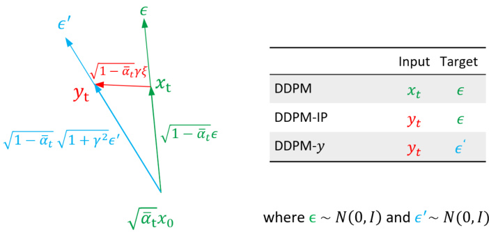
Figure 1. The inputs and the prediction targets are different in vanilla DDPM, DDPM-IP and DDPM- $\cdot y$ .
图 1: 原始 DDPM、DDPM-IP 和 DDPM-$\cdot y$ 的输入与预测目标存在差异。
5.3. Estimating the Prediction Error
5.3. 预测误差估计
In this section, we analyze the actual prediction error of $\epsilon_{\theta}(\cdot)$ and we use this analysis to choose the value of $\gamma$ in Eq. 6. Analogously to Sec. 4, we use ADM, trained using the standard algorithm Alg. 1 and two datasets: CIFAR10 and ImageNet $32\times32$ . At testing time, for a given $t$ and $\hat{\pmb{\epsilon}}=\pmb{\epsilon}{\pmb{\theta}}(\hat{\pmb{x}}{t},t)$ , we replace e with e in Eq. 4 and we compute the predicted $\hat{\pmb x}{0}$ . Finally, the prediction error at time $t$ is $\pmb{e}{t}=\hat{\pmb x}{0}-\pmb x_{0}$ . Note that using $\hat{\pmb x}{0}$ and $\pmb{x}{0}$ to estimate the error instead of comparing $\hat{\pmb x}{t}$ and $\pmb{x}{t}$ , has the advantage that the former is independent of scaling factors $(\sqrt{1-\bar{\alpha}{t}})$ and, thus, it makes the statistical analysis easier. Using different values of $t$ , uniformly selected in ${1,...,T}$ , we empirically verified that, for a given $t$ , $e_{t}$ is normally distributed: $e_{t}\sim$ $\mathcal{N}(\mathbf{0},\nu_{t}^{2}I)$ , with standard deviation $\nu_{t}$ (see Appendix A.5).
在本节中,我们分析 $\epsilon_{\theta}(\cdot)$ 的实际预测误差,并利用该分析选择公式6中 $\gamma$ 的值。与第4节类似,我们采用通过标准算法Alg. 1训练的ADM模型,分别在CIFAR10和ImageNet $32\times32$ 数据集上进行测试。测试时,对于给定的 $t$ 和 $\hat{\pmb{\epsilon}}=\pmb{\epsilon}{\pmb{\theta}}(\hat{\pmb{x}}{t},t)$ ,我们将公式4中的e替换为e来计算预测值 $\hat{\pmb x}{0}$ 。最终,时刻 $t$ 的预测误差为 $\pmb{e}{t}=\hat{\pmb x}{0}-\pmb x_{0}$ 。需要注意的是,使用 $\hat{\pmb x}{0}$ 和 $\pmb{x}{0}$ 而非 $\hat{\pmb x}{t}$ 与 $\pmb{x}{t}$ 来估计误差的优势在于:前者不受缩放因子 $(\sqrt{1-\bar{\alpha}{t}})$ 的影响,从而简化了统计分析。通过在 ${1,...,T}$ 中均匀选取不同的 $t$ 值,我们经验证发现对于给定 $t$ ,误差 $e_{t}$ 服从正态分布: $e_{t}\sim$ $\mathcal{N}(\mathbf{0},\nu_{t}^{2}I)$ ,其标准差为 $\nu_{t}$ (参见附录A.5)。
In Fig. 2 we plot the value of $\nu_{t}$ with respect to $t$ . The two curves corresponding to the two datasets are surprisingly close to each other. In principle, we could use this empirical analysis and set $\gamma_{t}=\nu_{t}$ in Eq. 6. In this way, when we perturb the input to $\epsilon_{\theta}(\cdot)$ , we empirically imitate its actual prediction error which is the base of the exposure bias problem. However, this choice would require a two-step training: first, using Alg. 1 to train the base model and empirically estimate $\nu_{t}$ for different $t$ . Then, using Alg. 3 with the estimated $\gamma_{t}$ schedule to retrain the model from scratch. To avoid this and make the whole procedure as simple as possible, we simply use a constant value $\gamma$ , independently of $t$ . This value was empirically set using a grid search on both CIFAR10 and ImageNet $32\times32$ on a small range of values covering the last half of the sampling trajectory. Specifically, we investigated the range $\nu_{t}\in[0,\mathbb{E}{t}[\nu_{t}]]=[0,0.2]$ (see Fig. 2), which was chosen following Karras et al. (2022), who showed that the last part of the inference trajectory has usually the largest impact on the Diffusion Model performance. We finally set $\gamma=0.1$ and, in the rest of this paper, we always use a constant $\gamma=0.1$ , regardless of the dataset and the baseline DDPM. Although a DDPM-specific $\gamma$ value would most likely lead to better quality results, we prefer to emphasise the ease of use of our proposal which does not depend on any other hyper parameter.
在图 2 中,我们绘制了 $\nu_{t}$ 随 $t$ 的变化曲线。两条对应不同数据集的曲线惊人地接近。理论上,我们可以利用这一实证分析结果,在公式 6 中设 $\gamma_{t}=\nu_{t}$。这样当我们对 $\epsilon_{\theta}(\cdot)$ 的输入施加扰动时,就能通过经验模拟其实际预测误差(这正是曝光偏差问题的根源)。但该方案需要分两步训练:首先使用算法 1 训练基础模型并经验性估算不同 $t$ 对应的 $\nu_{t}$,然后使用算法 3 配合估算出的 $\gamma_{t}$ 调度表从头开始重新训练模型。为简化流程,我们直接采用与 $t$ 无关的常量 $\gamma$。该值通过在 CIFAR10 和 ImageNet $32\times32$ 数据集上对采样轨迹后半段进行小范围网格搜索确定。具体而言,我们考察了 $\nu_{t}\in[0,\mathbb{E}{t}[\nu_{t}]]=[0,0.2]$ 区间(见图 2),该区间选择依据 Karras et al. (2022) 的研究——他们证明推理轨迹末段通常对扩散模型性能影响最大。最终我们设定 $\gamma=0.1$,且本文后续实验均固定使用该常量值(不区分数据集和基线 DDPM 模型)。虽然针对特定 DDPM 调整 $\gamma$ 可能获得更优结果,但我们更强调本方案的易用性——它不依赖任何其他超参数。
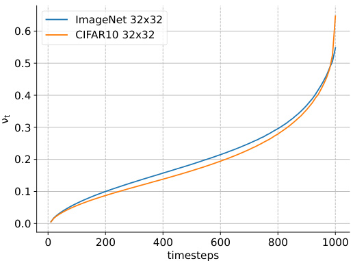
Figure 2. The inference time standard deviation $\nu_{t}$ of the prediction error of a pre-trained network with respect to the sampling step $t$ . The mean of the blue and the orange curve is 0.20 and 0.19, respectively.
图 2: 预训练网络预测误差的推理时间标准差 $\nu_{t}$ 与采样步长 $t$ 的关系。蓝色和橙色曲线的均值分别为 0.20 和 0.19。
5.4. Regular iz ation based on Lipschitz Continuous Functions
5.4. 基于Lipschitz连续函数的正则化
In this section, we propose two alternative solutions to the exposure bias problem which can help to better investigate the phenomenon. The goal is the same as in Sec. 5.1, i.e., we want to smooth the prediction function $\epsilon_{\theta}(\pmb{x}{t},t)$ to make it more robust with respect to local variations of $\pmb{x}{t}$ which are due to the inference-time prediction errors. To do so, instead of using input perturbation, we explicitly encourage $\epsilon_{\theta}(\cdot)$ to be Lipschitz continuous, i.e. to satisfy:
在本节中,我们提出了两种解决曝光偏差问题的替代方案,以帮助更好地研究这一现象。目标与第5.1节相同,即我们希望平滑预测函数 $\epsilon_{\theta}(\pmb{x}{t},t)$ ,使其对由推理时预测误差引起的 $\pmb{x}{t}$ 局部变化更具鲁棒性。为此,我们不使用输入扰动,而是明确鼓励 $\epsilon_{\theta}(\cdot)$ 满足Lipschitz连续性,即满足:
$$
||\epsilon_{\pmb\theta}({\pmb x},t)-\epsilon_{\pmb\theta}({\pmb y},t)||\leq K||{\pmb x}-{\pmb y}||,\forall({\pmb x},{\pmb y})
$$
$$
||\epsilon_{\pmb\theta}({\pmb x},t)-\epsilon_{\pmb\theta}({\pmb y},t)||\leq K||{\pmb x}-{\pmb y}||,\forall({\pmb x},{\pmb y})
$$
for a small constant $K$ . We implement this idea using two standard Lipschitz constant minimization methods: gradient penalty (Rifai et al., 2011; Gulrajani et al., 2017) and weight decay (Krogh & Hertz, 1991; Miyato et al., 2018). In both cases we do not perturb the input of $\epsilon_{\pmb{\theta}}(\cdot)$ , and we use the original training algorithm (Alg. 1), with the only difference being the loss function used in line 4, where the $L_{2}$ loss is used jointly with a regular iz ation term described below.
对于一个小的常数 $K$。我们采用两种标准的Lipschitz常数最小化方法实现这一思路:梯度惩罚 (Rifai et al., 2011; Gulrajani et al., 2017) 和权重衰减 (Krogh & Hertz, 1991; Miyato et al., 2018)。这两种情况下我们都不扰动 $\epsilon_{\pmb{\theta}}(\cdot)$ 的输入,且使用原始训练算法 (算法1),唯一区别在于第4行使用的损失函数,其中 $L_{2}$ 损失与下述正则化项联合使用。
Gradient penalty. In this case, the regular iz ation is based on the Frobenius norm of the Jacobian matrix (Rifai et al., 2011; Goodfellow et al., 2016), and the final loss is:
梯度惩罚 (Gradient penalty)。在这种情况下,正则化基于雅可比矩阵 (Jacobian matrix) 的 Frobenius 范数 (Rifai et al., 2011; Goodfellow et al., 2016),最终损失函数为:
$$
L_{G P}(\pmb\theta)=||\epsilon-\epsilon_{\pmb\theta}({\pmb x}{t},t)||^{2}+\lambda_{G P}\left|\frac{\partial\epsilon_{\pmb\theta}({\pmb x}{t},t)}{\partial{\pmb x}}\right|_{F}^{2},
$$
$$
L_{G P}(\pmb\theta)=||\epsilon-\epsilon_{\pmb\theta}({\pmb x}{t},t)||^{2}+\lambda_{G P}\left|\frac{\partial\epsilon_{\pmb\theta}({\pmb x}{t},t)}{\partial{\pmb x}}\right|_{F}^{2},
$$
where $\lambda_{G P}$ is the weight of the gradient penalty term. However, a gradient penalty regular iz ation is very slow (Yoshida & Miyato, 2017) because it involves one forward and two backward passes for each training step.
其中 $\lambda_{G P}$ 是梯度惩罚项的权重。然而,梯度惩罚正则化非常缓慢 (Yoshida & Miyato, 2017) ,因为每个训练步骤都需要一次前向传播和两次反向传播。
Weight decay. As shown in (Liu et al., 2022), Lipschitz continuity can also be encouraged using a weight decay regular iz ation (see Appendix A.6 for more details). In this case, the final loss is:
权重衰减。如 (Liu et al., 2022) 所示,权重衰减正则化也能促进 Lipschitz 连续性 (详见附录 A.6)。此时最终损失函数为:
$$
\begin{array}{r}{L_{W D}(\pmb{\theta})=||\pmb{\epsilon}-\pmb{\epsilon}{\pmb{\theta}}(\pmb{x}{t},t)||^{2}+\lambda_{W D}||\pmb{\theta}||^{2},}\end{array}
$$
$$
\begin{array}{r}{L_{W D}(\pmb{\theta})=||\pmb{\epsilon}-\pmb{\epsilon}{\pmb{\theta}}(\pmb{x}{t},t)||^{2}+\lambda_{W D}||\pmb{\theta}||^{2},}\end{array}
$$
where $\lambda_{W D}$ is the weight of the regular iz ation term.
其中 $\lambda_{W D}$ 是正则化项的权重。
6. Results
6. 结果
In this section, we evaluate the generation quality of the proposed solutions and we compare them with state-of-the-art DDPMs. We use unconditional image generation tasks on different datasets and standard metrics: the Fréchet Inception Distance (FID) (Heusel et al., 2017) and the Spatial Fréchet Inception Distance (sFID) (Nash et al., 2021). As a variant of FID, sFID uses spatial features rather than the standard pooled features to better capture spatial relationships, rewarding image distributions with a coherent high-level structure. As mentioned in Sec. 5.3, in all our experiments we use $\gamma=0.1$ without any dataset or baseline specific tuning of our only hyper parameter.
在本节中,我们评估所提出方案的生成质量,并将其与最先进的DDPM (Denoising Diffusion Probabilistic Models) 进行对比。我们在不同数据集上采用无条件图像生成任务及标准评估指标:Fréchet Inception Distance (FID) [20] 和 Spatial Fréchet Inception Distance (sFID) [21]。作为FID的变体,sFID通过使用空间特征而非标准池化特征来更好地捕捉空间关系,从而奖励具有连贯高层结构的图像分布。如第5.3节所述,所有实验均采用 $\gamma=0.1$ 的超参数设置,未针对任何数据集或基线进行特定调整。
6.1. Evaluation of the Different Proposed Solutions
6.1. 不同提案解决方案的评估
In this section, we empirically compare to each other the three regular iz ation methods proposed in Sec. 5 to alleviate the exposure bias problem. For all three approaches, we use the state-of-the-art diffusion model ADM (Dhariwal & Nichol, 2021) (without classifier guidance) as the baseline, and we call: (1) “ADM-IP” the version of ADM trained using Alg. 3, (2) “ADM-GP” the version of ADM trained using the gradient penalty, and (3) “ADM-WD” for the weight decay (Sec. 5.4). We use $\lambda_{G P}=1e-6$ and $\lambda_{W D}=0.03$ as the loss weights for ADM-GP and ADM-WD, respectively.
在本节中,我们通过实验对比第5章提出的三种缓解曝光偏差问题的正则化方法。所有实验均以最先进的扩散模型ADM (Dhariwal & Nichol, 2021) (无分类器引导) 为基线,并命名如下: (1) "ADM-IP" 表示采用算法3训练的ADM版本, (2) "ADM-GP" 表示采用梯度惩罚训练的ADM版本, (3) "ADM-WD" 表示采用权重衰减的版本 (第5.4节)。实验中设置ADM-GP的损失权重 $\lambda_{G P}=1e-6$,ADM-WD的损失权重 $\lambda_{W D}=0.03$。
For this experiment, we use CIFAR10 because ADM-GP is too time-consuming to be trained on larger datasets. The results in Tab. 2 show that all three models outperform the baseline in image quality, demonstrating the effectiveness of smoothing the prediction function using the proposed regular iz ation methods. However, training ADM-GP is too slow and cannot be scaled to larger datasets, thus we do not recommend this solution. Moreover, ADM-IP gets the best FID and sFID scores, thus, in the rest of this paper, we use the input perturbation approach described in Sec. 5.1 as our basic solution.
本次实验选用CIFAR10数据集,因为ADM-GP在更大规模数据集上的训练耗时过高。表2结果显示,三种模型在图像质量指标上均超越基线,验证了通过所提正则化方法平滑预测函数的有效性。但ADM-GP训练速度过慢且难以扩展至更大数据集,因此不建议采用该方案。此外,ADM-IP取得了最优的FID和sFID分数,故本文后续将采用5.1节所述的输入扰动方法作为基础解决方案。
Table 2. Comparison of different regular iz ation methods. All the models are tested using $T=1,000$ sampling steps.
表 2: 不同正则化方法的对比。所有模型均使用 $T=1,000$ 采样步数进行测试。
| Model | CIFAR10 32×32 |
|---|---|
| FID sFID | |
| ADM (baseline) | 2.99 4.76 |
| ADM-GP | 2.80 4.41 |
| ADM-WD | 2.82 4.61 |
| ADM-IP | 2.76 4.05 |
Finally, we use ADM-IP to quantify the reduction in the exposure bias following the protocol described in Sec. 4. The results reported in Tab. 1 show that ADM-IP leads to a significantly lower exposure bias than ADM, and this difference is larger with longer sampling sequences.
最后,我们按照第4节描述的方案使用ADM-IP来量化曝光偏差的减少。表1所示结果表明,ADM-IP导致的曝光偏差显著低于ADM,且采样序列越长,这种差异越大。
6.2. Main results
6.2. 主要结果
Comparison with DDPMs. We compare ADM-IP with ADM using CIFAR10, ImageNet $32\times32$ , LSUN tower $64\times64$ , CelebA $64\times64$ (Liu et al., 2015) and FFHQ $128\times128$ . Following prior work (Ho et al., 2020; Nichol & Dhariwal, 2021), we generate 50K samples for each trained model and we use the full training set to compute the reference distribution statistics, except for LSUN tower where (again following (Ho et al., 2020; Nichol & Dhariwal, 2021)) we use 50K training samples as the reference data. When training, we always use $T=1,000$ steps for all the models. At inference time, the results reported with $T^{\prime}<T$ sampling steps have been obtained using the respacing technique (Nichol & Dhariwal, 2021). As previously mentioned (see Sec. 5.3) we keep fixed $\gamma=0.1$ in all the experiments and the datasets. We refer to Appendix A.7 for the complete list of hyper parameters (e.g. the learning rate, the batch size, etc.) and network architecture settings, which are the same for both ADM and ADM-IP.
与DDPM的对比。我们将ADM-IP与ADM在CIFAR10、ImageNet $32\times32$、LSUN tower $64\times64$、CelebA $64\times64$ (Liu et al., 2015) 和 FFHQ $128\times128$ 数据集上进行对比。遵循先前工作 (Ho et al., 2020; Nichol & Dhariwal, 2021),我们为每个训练模型生成5万样本,并使用完整训练集计算参考分布统计量(LSUN tower除外,此处沿用 (Ho et al., 2020; Nichol & Dhariwal, 2021) 方法,采用5万训练样本作为参考数据)。训练时,所有模型均使用 $T=1,000$ 步。推理阶段,$T^{\prime}<T$ 采样步数的结果通过重间距技术 (Nichol & Dhariwal, 2021) 获得。如第5.3节所述,所有实验和数据集中固定 $\gamma=0.1$。完整超参数列表(如学习率、批次大小等)及网络架构设置(ADM与ADM-IP相同)详见附录A.7。
The results reported in Tab. 3 show that, independently of the dataset and the number of sampling steps $(T^{\prime}\leq T)$ , ADM-IP is always better than ADM in terms of both the FID and sFID metrics, sometimes drastically better. For instance, on LSUN, with $T^{\prime}=80$ , we have a more than 5 sFID score improvement with respect to ADM. On FFHQ $128\times128$ , with $T^{\prime}=1,000$ , we have almost 7 points of improvement compared to both the FID and the sFID scores. In addition to the experiments shown in Tab. 3, we used $T^{\prime}=900$ sampling steps and our ADM-IP on CelebA $64\times64$ , achieving a result of 1.27 FID, which is the new state-of-the-art performance for unconditional generation on this dataset.
表 3 中的结果表明,无论数据集和采样步数 $(T^{\prime}\leq T)$ 如何,ADM-IP 在 FID 和 sFID 指标上始终优于 ADM,有时甚至显著领先。例如,在 LSUN 数据集上,当 $T^{\prime}=80$ 时,ADM-IP 的 sFID 分数比 ADM 提高了 5 分以上。在 FFHQ $128\times128$ 数据集上,当 $T^{\prime}=1,000$ 时,FID 和 sFID 分数均提升了近 7 分。除表 3 所示的实验外,我们还使用 $T^{\prime}=900$ 采样步数和 ADM-IP 在 CelebA $64\times64$ 数据集上取得了 1.27 的 FID 分数,这是该数据集无条件生成任务的最新最优性能。
Table 3. Comparison between ADM and ADM-IP using models trained with $T=1,000$ sampling steps and tested with $T^{\prime}\leq T$ steps.
表 3. 使用 $T=1,000$ 采样步长训练并以 $T^{\prime}\leq T$ 步长测试的 ADM 与 ADM-IP 模型对比。
| 采样步长 (T') | 模型 | CIFAR10 | ImageNet 32 | LSUN tower 64 | CelebA 64 | FFHQ 128 | |||||
|---|---|---|---|---|---|---|---|---|---|---|---|
| FID | sFID | FID | sFID | FID | sFID | FID | sFID | FID | sFID | ||
| 1,000 | ADM (baseline) | 2.99 | 4.76 | 3.60 | 3.30 | 3.39 | 7.96 | 1.60 | 3.80 | 9.65 | 12.53 |
| ADM-IP (ours) | 2.76 | 4.05 | 2.87 | 2.39 | 2.68 | 6.04 | 1.31 | 3.38 | 2.98 | 5.59 | |
| 300 | ADM | 2.95 | 4.95 | 3.58 | 3.48 | 3.31 | 8.39 | 1.82 | 4.25 | 9.55 | 12.60 |
| ADM-IP | 2.67 | 4.14 | 2.74 | 2.58 | 2.60 | 5.98 | 1.43 | 3.36 | 3.74 | 5.97 | |
| 100 | ADM | 3.37 | 5.66 | 4.26 | 4.48 | 3.50 | 11.10 | 3.02 | 5.76 | 14.52 | 16.02 |
| ADM-IP | 2.70 | 4.51 | 3.24 | 3.13 | 2.79 | 6.56 | 2.21 | 4.33 | 5.94 | 7.90 | |
| 80 | ADM | 3.63 | 5.97 | 4.61 | 4.76 | 4.17 | 12.60 | 3.75 | 6.80 | 17.00 | 18.02 |
| ADM-IP | 2.93 | 4.69 | 3.57 | 3.33 | 2.95 | 6.93 | 2.67 | 4.69 | 6.89 | 8.79 |
Note that, for most datasets, both the baseline (ADM) and ADM-IP reach the best results with $T^{\prime}<T$ (specifically, with $T^{\prime}\in[100,300])$ . As mentioned in Sec. 4, this is most likely a confirmation of the exposure bias problem: a shorter sampling trajectory accumulates a smaller prediction error.
需要注意的是,对于大多数数据集,基线方法 (ADM) 和 ADM-IP 都在 $T^{\prime}<T$(具体而言,$T^{\prime}\in[100,300]$)时达到最佳效果。如第4节所述,这很可能印证了曝光偏差问题:较短的采样轨迹会累积更小的预测误差。
Besides generating significantly better images, ADM-IP converges much faster than the baseline during training in all the five datasets (see Fig. 3 and 4). For instance, on LSUN tower and CelebA, ADM-IP converges at 220K and 300K training iterations while ADM saturates around 300K and 480K iterations, respectively. Fig. 3 shows also that, even before convergence, ADM-IP quickly beats the ADM results obtained when the latter has converged. For instance, on CelebA, ADM-IP gets FID 1.51 at 120K training iterations, whereas ADM gets FID 1.6 at convergence (480K iterations), exhibiting a $4\mathbf{x}$ training speed-up. On the larger resolution FFHQ dataset, ADM receives FID 14.52 at convergence (420K iterations), while ADM-IP achieves a FID score of 8.81 with only 60K iterations: an improvement of 5.71 points with a $7\mathbf{x}$ training speed-up. Fig. 4 shows a similar trend for the CIFAR10 dataset. In this figure, we also plot the results of ADM-IP with different $\gamma$ values (Sec. 5.3).
除了生成质量显著更优的图像外,ADM-IP在所有五个数据集的训练过程中收敛速度都远快于基线方法(见图3和4)。例如在LSUN tower和CelebA数据集上,ADM-IP分别在22万次和30万次训练迭代时收敛,而ADM的收敛点约为30万次和48万次迭代。图3还显示,即使在收敛之前,ADM-IP也能快速超越ADM收敛后的结果。以CelebA为例,ADM-IP在12万次迭代时就取得FID 1.51,而ADM在收敛时(48万次迭代)的FID为1.6,实现了4倍训练加速。在更高分辨率的FFHQ数据集上,ADM收敛时(42万次迭代)的FID为14.52,而ADM-IP仅用6万次迭代就达到FID 8.81,在提升5.71个指标点的同时实现7倍训练加速。图4展示了CIFAR10数据集上的相似趋势,该图中我们还绘制了不同γ取值下ADM-IP的结果(见5.3节)。
The training iterations until convergence for each model are summarized in Tab. 4. The much faster convergence of our method is most likely due to the regular iz ation effect of the input perturbation. In fact, as commonly happens with regularization techniques (Zhang et al., 2018; Liu et al., 2021;
各模型直至收敛的训练迭代次数总结如表 4 所示。我们方法的更快收敛很可能归因于输入扰动 (input perturbation) 的正则化效应。事实上,正如正则化技术常见的情况 (Zhang et al., 2018; Liu et al., 2021;
Bales trier o et al., 2022), the proposed input perturbation also introduces an inductive bias in training. In our case, it is: close points in the domain of the prediction function should lead to similar outcomes. Our empirical results show that this bias helps the DDPM training.
Bales trier o等人(2022)提出的输入扰动方法也在训练中引入了归纳偏置。在我们的案例中表现为:预测函数定义域内相邻的点应当产生相似输出。实证结果表明这种偏置有助于DDPM训练。
Tab. 4 also shows that ADM-IP can drastically accelerate the inference process, i.e. obtaining better results than the baseline with shorter sampling trajectories. For example, with only 60 or 80 steps, ADM-IP gets a better or an equivalent FID than ADM (tested with the standard 1,000 sampling steps) on all datasets, except for CelebA, where ADM-IP needs 200 sampling steps to reach the same result. This comparison shows a remarkable 5x to $16.7\mathbf{X}$ speed-up of the inference stage, which is particularly significant for the larger resolution FFHQ dataset.
表 4 还显示,ADM-IP 能大幅加速推理过程,即在更短的采样轨迹下获得比基线更好的结果。例如,仅用 60 或 80 步时,ADM-IP 在所有数据集上的 FID 均优于或等同于 ADM (标准测试采用 1,000 采样步数) ,仅在 CelebA 数据集上需要 200 采样步才能达到相同结果。这一对比显示出推理阶段实现了惊人的 5 倍至 $16.7\mathbf{X}$ 加速,对于更高分辨率的 FFHQ 数据集尤为显著。
Finally, we measure the recall and precision for the generated samples using the method in Ky nk a an niemi et al. (2019). The results show that the recall and precision achieved by ADM and ADM-IP have no significant difference, which indicates that our input perturbation does not affect the sample diversity (see Appendix A.4).
最后,我们采用Ky nk a an niemi等人 (2019) 的方法测量生成样本的召回率与精确度。结果表明ADM与ADM-IP取得的召回率和精确度无显著差异,这说明我们的输入扰动不会影响样本多样性 (详见附录A.4)。
Comparison with DDIMs. In order to show the generality of our proposal, we use Alg. 3 with the Denoising Diffusion Implicit Models (DDIMs) proposed by Song et al. (2021a) (Sec. 2). We train both the baseline (DDIM) and our method (DDIM-IP) on CIFAR10 using the public code provided by Song et al. (2021a). Since training with DDIM is particularly slow, we use only CIFAR10 for this comparison. We use the default hyper parameters settings (e.g. $T=1,000;$ ) in their code and train both models for 1,600K iterations with batch size 128. We test the performance of the two models with both $\eta=0$ and $\eta=0.5$ , where $\eta$ is the coefficient of stochastic it y sampling in DDIMs. Also in this case, for our method (DDIM-IP) we use $\gamma=0.1$ without any fine-tuning.
与DDIMs的对比。为展示我们方案的通用性,我们采用Song等人(2021a)(第2节)提出的去噪扩散隐式模型(DDIMs)结合算法3进行实验。使用Song等人(2021a)公开代码在CIFAR10数据集上同时训练基线模型(DDIM)和我们的方法(DDIM-IP)。由于DDIM训练速度极慢,本次对比仅使用CIFAR10数据集。我们沿用代码默认超参数设置(如$T=1,000;$),以128的批次大小训练两个模型160万次迭代。测试时分别采用$\eta=0$和$\eta=0.5$两种配置($\eta$表示DDIMs中随机采样的系数)。本实验中我们的方法(DDIM-IP)直接采用$\gamma=0.1$参数,未进行任何微调。

Figure 3. FID scores with respect to the number of training iterations. Each FID value is computed using $T^{\prime}=1,000$ inference sampling steps, except for the FFHQ dataset, for which we used $T^{\prime}=100$ .
图 3: 不同训练迭代次数下的FID分数。除FFHQ数据集使用 $T^{\prime}=100$ 外,其余FID值均基于 $T^{\prime}=1,000$ 次推理采样步骤计算。

Figure 4. CIFAR10: FID scores with respect to the number of training iterations with different $\gamma$ values. Each FID score is computed using $T^{\prime}=100$ inference sampling steps.
图 4: CIFAR10: 不同γ值下FID分数随训练迭代次数的变化。每个FID分数均使用T′=100推理采样步数计算。
We report the results in Tab. 5, which show that DDIM-IP consistently obtains better FID scores than DDIM in all conditions (i.e., independently of the number of sampling steps and the value of $\eta$ ). Importantly, the fewer the sampling steps, the more the FID gain which is obtained with input perturbation. For instance, with $\eta=0.5$ , the FID gain of DDIM-IP is 7.16 with 10 sampling steps versus 0.89 with 1,000 sampling steps. Analogously, with $\eta:=:0$ and 10 sampling steps, DDIM-IP drastically improves DDIM with a 3.67 FID margin. Since the main advantage of DDIMs with respect to DDPMs is their reduced number of sampling steps (Song et al., 2021a), and they indeed are mainly used for accelerating the inference stage, input perturbation greatly matches this goal, and it significantly improves the sample quality of the implicit models in a short sampling sequence regime.
我们在表5中报告了结果,这些结果表明在所有条件下(即无论采样步数和$\eta$值如何)DDIM-IP始终比DDIM获得更好的FID分数。重要的是,采样步数越少,输入扰动带来的FID增益就越大。例如,当$\eta=0.5$时,DDIM-IP在10个采样步数下的FID增益为7.16,而在1,000个采样步数下仅为0.89。类似地,当$\eta=0$且采样步数为10时,DDIM-IP以3.67的FID差距显著优于DDIM。由于DDIM相对于DDPM的主要优势在于减少了采样步数(Song等人,2021a),并且它们确实主要用于加速推理阶段,因此输入扰动非常符合这一目标,并在短采样序列机制中显著提高了隐式模型的样本质量。
7. Conclusions
7. 结论
In this paper, we proposed DDPM-IP, a regular iz ation method for DDPM training which is based on input perturbation to explicitly model the prediction errors and alleviate the DDPM exposure bias problem. We empirically showed that DDPM-IP can significantly improve image quality and drastically reduce both the training and the inference time. The proposed method is straightforward and does not require any change in the network architecture or the specific loss function. This simplicity makes it very easy to be reproduced and plugged into existing DDPMs. Although we tested DDPM-IP only on an image domain, there are no domain-specific assumptions behind our method, hence we presume it can be more generally applied to other domains.
本文提出了DDPM-IP,这是一种基于输入扰动 (input perturbation) 的DDPM训练正则化方法,旨在显式建模预测误差并缓解DDPM的曝光偏差问题。实验表明,DDPM-IP能显著提升图像质量,并大幅减少训练和推理时间。该方法实现简单,无需改变网络架构或特定损失函数,这种简洁性使其易于复现并嵌入现有DDPM框架。尽管我们仅在图像领域测试了DDPM-IP,但该方法不依赖领域特定假设,因此我们推测其可更广泛地应用于其他领域。
Table 4. ADM-IP training and testing acceleration. Note that, for a single training iteration, ADM and ADM-IP take exactly the same amount of time, and the same is true for a single sampling step.
表 4: ADM-IP训练与测试加速。需注意,对于单次训练迭代,ADM和ADM-IP耗时完全相同,单次采样步骤亦是如此。
| 数据集 | 模型 | 训练迭代次数 | 采样步骤 | FID |
|---|---|---|---|---|
| CIFAR10 32×32 | ADM | 500K | 1,000 | 2.99 |
| ADM-IP | 460K | 80 | 2.93 | |
| ImageNet 32×32 | ADM | 4500K | 1,000 | 3.53 |
| LSUN tower 32×32 | ADM-IP | 4000K | 80 | 3.50 |
| ADM | 300K | 1,000 | 3.39 | |
| 64×64 | ADM-IP | 220K | 60 | 3.31 |
| CelabA 64×64 | ADM | 480K | 1,000 | 1.60 |
| ADM-IP | 300K | 200 | 1.53 | |
| FFHQ 128×128 | ADM | 420K | 1,000 | 9.65 |
| ADM-IP | 180K | 60 | 8.72 |
Table 5. CIFAR10: Comparison between DDIM and DDIM-IP using models trained with $T=1$ , 000 sampling steps and tested with $T^{\prime}\leq T$ steps.
表 5. CIFAR10: DDIM与DDIM-IP的对比,使用采样步数 $T=1$,000训练的模型,并在 $T^{\prime}\leq T$ 步数下测试。
| m1 | Model | Sampling steps (T') |
|---|---|---|
| 10 | ||
| 0 | DDIM | 14.21 |
| 0.5 | DDIM-IP DDIM | 10.54 |
| DDIM-IP | 17.24 10.06 |
Limitations. Since training DDPMs is very computationally heavy, in this paper we used only datasets with small resolution images. We leave the extension of our experiments to larger resolution images (and corresponding larger backbone networks) as a future work. However, we emphasize that our best results have been obtained with FFHQ $128\times128$ , which is the dataset with the largest resolution images we tested, which probably confirms that our regularization method is specifically effective with higher dimensional input spaces.
局限性。由于训练DDPM的计算量非常大,本文仅使用了低分辨率图像数据集。我们将实验扩展到更高分辨率图像(及相应更大的骨干网络)作为未来工作。但需要强调的是,我们的最佳结果是在FFHQ $128\times128$ 数据集上取得的,这是我们测试过的最高分辨率图像数据集,这可能证实了我们的正则化方法在高维输入空间中具有特殊效果。
Acknowledgments
致谢
This work has been supported by the European Union’s Horizon 2020 research and innovation programme under the Marie Skłodowska-Curie grant agreement No 955778. Moreover, we acknowledge the CINECA award under the
本研究获得欧盟"地平线2020"科研创新计划玛丽·斯克沃多夫斯卡-居里资助协议(No 955778)支持。同时感谢CINECA项目资助。
ISCRA initiative, for the availability of high-performance computing resources and support.
ISCRA计划,用于高性能计算资源的可用性及支持。
A. Appendix
A. 附录
A.1. Exposure Bias Analysis
A.1. 曝光偏差分析
In this section, we repeat the experiment in Sec. 4 by removing the randomness component of the sampling process in order to isolate the error of the reverse process which is due only to the prediction network. Specifically, we use again ADM (Dhariwal & Nichol, 2021) (trained with $T=1,000;$ ) and ImageNet $32\times32$ , and we directly measure the difference between a ground truth real image $\pmb{x}{0}$ and the predicted $\hat{\pmb x}{0}$ using a deterministic sampling, described in Alg. 4. In more detail, given a real image $\pmb{x}{0}$ , we first compute $\pmb{x}{t}$ by Eq. 4, then we use the pre-trained network $\epsilon_{\pmb{\theta}}$ (trained with the standard algorithm Alg. 1) to run the reverse diffusion for $t$ steps. Note that we adopt the equation in line 4 of Alg. 2 but we remove the stochastic term $\sigma_{t}\pm$ . Differently from the analogous experiment presented in Sec. 4, this deterministic reverse diffusion process allows the model to target the mode of $\pmb{x}{0}$ instead of favouring diversity (Luo, 2022). Finally, we use the average pixel-wise $L_{1}$ distance between $\pmb{x}{0}$ and $\hat{\pmb x}_{0}$ to estimate the cumulative error computed in the whole trajectory of $t$ steps. Note that, since each pixel is normalized in $[-1,1]$ (Sec. 3), then this distance is upper bounded by 2.
在本节中,我们复现了第4章的实验,通过移除采样过程中的随机性成分来单独分析仅由预测网络导致的反向过程误差。具体而言,我们再次使用ADM (Dhariwal & Nichol, 2021) (训练步长$T=1,000;$ )和ImageNet $32\times32$数据集,并采用算法4描述的确定性采样方法,直接测量真实图像$\pmb{x}{0}$与预测图像$\hat{\pmb x}{0}$之间的差异。详细流程如下:给定真实图像$\pmb{x}{0}$,先通过公式4计算$\pmb{x}{t}$,再使用预训练网络$\epsilon_{\pmb{\theta}}$ (基于标准算法1训练)执行$t$步反向扩散。需要注意的是,我们采用算法2第4行的方程但移除了随机项$\sigma_{t}\pm$。与第4章的对比实验不同,这种确定性反向扩散过程使模型能够瞄准$\pmb{x}{0}$的模态而非追求多样性 (Luo, 2022)。最终,我们通过$\pmb{x}{0}$与$\hat{\pmb x}{0}$之间的平均像素级$L_{1}$距离来估计$t$步完整轨迹的累积误差。由于每个像素值被归一化至$[-1,1]$区间 (第3章),该距离的理论上限为2。
Algorithm 4 Deterministic measurement of exposure bias
算法 4 曝光偏差的确定性测量
In Tab. 6, we report the exposure bias measured using $\bar{\delta_{t}}$ with respect to different trajectory lengths $(t)$ . This table shows that the error accumulates greatly as the number of reverse diffusion steps increases. In Fig. 5 we visualize a few pairs of images $(\pmb{x}{0},\hat{\pmb{x}}_{0})$ with the corresponding length of the diffusion trajectory $(t)$ . These images clearly show how large the error is accumulated with the diffusion chain getting longer.
在表6中,我们报告了使用$\bar{\delta_{t}}$测量的曝光偏差与不同轨迹长度$(t)$的关系。该表显示,随着反向扩散步骤数量的增加,误差会大幅累积。在图5中,我们可视化了几对图像$(\pmb{x}{0},\hat{\pmb{x}}_{0})$及其对应的扩散轨迹长度$(t)$。这些图像清晰地展示了随着扩散链变长,误差累积的程度有多大。
Table 6. A deterministic estimate of the exposure bias $(\bar{\delta_{t}})$ with respect to different lengths of the reverse diffusion trajectory. The error is upper bounded by 2.
表 6: 针对反向扩散轨迹不同长度的曝光偏差 $(\bar{\delta_{t}})$ 确定性估计。误差上限为2。
| 模型 | 反向扩散步数 |
|---|---|
| 100 | |
| ADM | 0.0539 |
A.2. Distribution of the Perturbed Input
A.2. 扰动输入的分布
In this section, we prove that $\pmb{y}{t}$ is Gaussian distributed as described in Eq. 7. Generally speaking, if $A\sim\mathcal N(\mu_{A},\sigma_{A}^{2})$ and $B\sim\mathcal N(\mu_{B},\sigma_{B}^{2})$ are two independent Gaussian distributed random variables, then its linear combination $S=a A+b B$ (with $a,b$ two scalars) is also Gaussian distributed:
在本节中,我们证明 $\pmb{y}{t}$ 如式7所述服从高斯分布。一般而言,若 $A\sim\mathcal N(\mu_{A},\sigma_{A}^{2})$ 和 $B\sim\mathcal N(\mu_{B},\sigma_{B}^{2})$ 是两个独立的高斯分布随机变量,则其线性组合 $S=a A+b B$ (其中 $a,b$ 为标量) 同样服从高斯分布:
$$
S\sim\mathcal{N}(a\mu_{A}+b\mu_{B},a^{2}\sigma_{A}^{2}+b^{2}\sigma_{B}^{2}).
$$
$$
S\sim\mathcal{N}(a\mu_{A}+b\mu_{B},a^{2}\sigma_{A}^{2}+b^{2}\sigma_{B}^{2}).
$$
In our case, we have that, for a given ${\pmb x}{0},{\pmb y}{t}$ is a linear combination of $\pmb{x}_{t}$ and $\xi$ , which are two independent, Gaussian distributed random variables:
在我们的案例中,对于给定的 ${\pmb x}{0}$,${\pmb y}{t}$ 是 $\pmb{x}_{t}$ 和 $\xi$ 的线性组合,这两个变量是独立且服从高斯分布的随机变量:

Figure 5. Visualization of the exposure bias problem with different diffusion chain lengths.
图 5: 不同扩散链长度下曝光偏差问题的可视化。
$$
\begin{array}{r}{q(\pmb{x}{t}|\pmb{x}{0})=\mathcal{N}(\pmb{x}{t};\sqrt{\bar{\alpha}{t}}\pmb{x}{0},(1-\bar{\alpha}{t})\pmb{I}),}\ {\pmb{\xi}\sim\mathcal{N}(\pmb{0},\pmb{I}),}\ {\pmb{y}{t}=\pmb{x}{t}+\sqrt{1-\bar{\alpha}_{t}}\gamma\pmb{\xi}.}\end{array}
$$
$$
\begin{array}{r}{q(\pmb{x}{t}|\pmb{x}{0})=\mathcal{N}(\pmb{x}{t};\sqrt{\bar{\alpha}{t}}\pmb{x}{0},(1-\bar{\alpha}{t})\pmb{I}),}\ {\pmb{\xi}\sim\mathcal{N}(\pmb{0},\pmb{I}),}\ {\pmb{y}{t}=\pmb{x}{t}+\sqrt{1-\bar{\alpha}_{t}}\gamma\pmb{\xi}.}\end{array}
$$
Hence, if in Eq. 12 we replace $S$ with $\pmb{y}{t},A$ with $\scriptstyle{\pmb{x}}{t}$ , $B$ with $\xi$ , and we use $a=1$ and $b=\sqrt{1-\bar{\alpha}_{t}}\gamma$ , we get:
因此,如果在方程 12 中将 $S$ 替换为 $\pmb{y}{t}$,$A$ 替换为 $\scriptstyle{\pmb{x}}{t}$,$B$ 替换为 $\xi$,并设 $a=1$ 和 $b=\sqrt{1-\bar{\alpha}_{t}}\gamma$,则可得到:
$$
\begin{array}{r}{q({\pmb y}{t}|{\pmb x}{0})=\mathcal{N}({\pmb y}{t};\sqrt{\bar{\alpha}{t}}{\pmb x}{0},(1-\bar{\alpha}{t}){\pmb I}+\gamma^{2}(1-\bar{\alpha}{t}){\pmb I})=}\ {=\mathcal{N}({\pmb y}{t};\sqrt{\bar{\alpha}{t}}{\pmb x}{0},(1-\bar{\alpha}_{t})(1+\gamma^{2}){\pmb I}).}\end{array}
$$
$$
\begin{array}{r}{q({\pmb y}{t}|{\pmb x}{0})=\mathcal{N}({\pmb y}{t};\sqrt{\bar{\alpha}{t}}{\pmb x}{0},(1-\bar{\alpha}{t}){\pmb I}+\gamma^{2}(1-\bar{\alpha}{t}){\pmb I})=}\ {=\mathcal{N}({\pmb y}{t};\sqrt{\bar{\alpha}{t}}{\pmb x}{0},(1-\bar{\alpha}_{t})(1+\gamma^{2}){\pmb I}).}\end{array}
$$
A.3. Ablation Study: Input Perturbation is not Equivalent to Using a Different Noise Variance
A.3. 消融研究:输入扰动不等同于使用不同噪声方差
The goal of this section is to empirically show that DDPM-IP is not equivalent to using a standard DDPM algorithm with a different noise distribution. Following the discussion in Sec. 5.2, and adopting the same terminology, we compare DDPM-IP with DDPM $\cdot y$ , where the latter is trained using the standard algorithm (Alg. 1) but adopting the noise distribution of ${\pmb y}_{t}$ . Tab. 7 shows that DDPM $\cdot y$ is even worse than DDPM.
本节旨在通过实验证明DDPM-IP与采用不同噪声分布的标准DDPM算法并不等效。根据第5.2节的讨论并沿用相同术语,我们将DDPM-IP与DDPM$\cdot y$进行对比(后者采用标准算法(算法1)训练,但使用${\pmb y}_{t}$的噪声分布)。表7显示DDPM$\cdot y$的表现甚至逊于标准DDPM。
Table 7. CIFAR10: comparing DDPM, DDPM $_y$ and DDPM-IP using different numbers of revers diffusion steps.
表 7. CIFAR10: 比较 DDPM、DDPM $_y$ 和 DDPM-IP 在不同反向扩散步数下的表现。
| 模型 | 输入 | 目标 | 80 步 FID | 80 步 sFID | 100 步 FID | 100 步 sFID | 300 步 FID | 300 步 sFID | 1000 步 FID | 1000 步 sFID |
|---|---|---|---|---|---|---|---|---|---|---|
| DDPM | 3t | E | 3.63 | 5.97 | 3.37 | 5.66 | 2.95 | 4.95 | 2.99 | 4.76 |
| DDPM-y | yt | E' | 4.24 | 6.51 | 3.90 | 6.23 | 3.21 | 5.39 | 3.25 | 5.04 |
| DDPM-IP | yt | E | 2.93 | 4.69 | 2.70 | 4.51 | 2.67 | 4.14 | 2.76 | 4.05 |
A.4. Recall and Precision
A.4. 召回率与精确率
We compare Recall and Precision for ADM and ADM-IP using the improved metrics (Ky nk a an niemi et al., 2019) and the code of Dhariwal & Nichol (2021). For each dataset and model, we generate 50,000 samples with 1,000 sampling steps. The results in Tab. 8 indicate that the Recall and Precision values achieved by ADM and ADM-IP have no significant difference, while ADM-IP gets slightly better results on CIFAR10 $32\times32$ and FFHQ $128\times128$ . Note that, due to the limited memory of our NVIDIA V100 16G GPU, we experienced an out-of-memory issue when computing Recall and Precision on the ImageNet $32\times32$ dataset, thus this result is not reported in Tab. 8.
我们采用改进后的指标 (Ky nk a an niemi等人, 2019) 和 Dhariwal & Nichol (2021) 的代码,对比了ADM和ADM-IP的召回率(Recall)与精确率(Precision)。针对每个数据集和模型,我们以1,000次采样步长生成了50,000个样本。表8结果显示,ADM与ADM-IP取得的召回率和精确率数值无显著差异,但ADM-IP在CIFAR10 $32\times32$ 和FFHQ $128\times128$ 数据集上略胜一筹。需要注意的是,由于NVIDIA V100 16G GPU的显存限制,我们在计算ImageNet $32\times32$ 数据集的召回率和精确率时遇到了内存溢出问题,因此该结果未在表8中呈现。
Table 8. Comparing Recall and Precision for ADM and ADM-IP on the four datasets using 1,000 sampling steps.
表 8: 在四个数据集上使用1,000采样步骤比较ADM和ADM-IP的召回率(Recall)和精确率(Precision)。
| 模型 | CIFAR10 32×32 | LSUN tower 64×64 | CelebA 64x64 | FFHQ 128×128 | ||||
|---|---|---|---|---|---|---|---|---|
| 召回率 | 精确率 | 召回率 | 精确率 | 召回率 | 精确率 | 召回率 | 精确率 | |
| ADM | 0.600 | 0.690 | 0.618 | 0.631 | 0.592 | 0.703 | 0.583 | 0.690 |
| ADM-IP | 0.606 | 0.696 | 0.612 | 0.640 | 0.601 | 0.700 | 0.585 | 0.703 |
A.5. Gaussian Prediction Error
A.5. 高斯预测误差
In this section, we use ImageNet $32\times32$ to empirically show that $\pmb{e}{t}\sim\mathcal{N}(\mathbf0,\nu_{t}^{2}I)$ (Sec. 5.3), i.e., that the prediction error is nearly isotropic Gaussian distributed. To do so, we need to prove that, for each $t$ and each input dimension (i.e., for each pixel and color channel) $i\in{1,...,M}$ , the pixel-wise error $(e_{t}^{i})$ follows $e_{t}^{i}\sim\mathcal N(0,\nu_{t}^{2})$ . To test this hypothesis, we uniformly select a subset of $100t$ values in ${1,...,T}$ using a stride of 10. Then, for each $t$ , we use 10K images and all the pixels to compute the pixel independent mean $\mu_{t}$ and variance $\nu_{t}^{2}$ of the error, which we use to standardize the error values for all the pixels $e_{t}^{i}$ (i.e., $\begin{array}{r}{\bar{e}{t}^{i}=\frac{e_{t}^{i}-\mu_{t}}{\nu_{t}^{2}},}\end{array}$ . Then, for each $i$ , we use 50 randomly selected $\bar{e}{t}^{i}$ values and the Shapiro–Wilk test (Shapiro & Wilk, 1965) to verify that they follow a standard normal distribution. The confidence level is set at $95%$ and we reject the null hypothesis if the $\mathsf{p}$ -value is less than 0.05. The null hypothesis was rejected only in a small minority of cases, confirming that the error $e_{t}$ is almost isotropic Gaussian distributed. Fig. 6 shows a few histogram examples for $e_{t}^{i}$ computed at different pixels.
在本节中,我们使用ImageNet $32\times32$ 数据集通过实验证明 $\pmb{e}{t}\sim\mathcal{N}(\mathbf0,\nu_{t}^{2}I)$ (第5.3节),即预测误差几乎呈各向同性高斯分布。为此,我们需要证明对于每个 $t$ 和每个输入维度(即每个像素和颜色通道) $i\in{1,...,M}$,像素级误差 $(e_{t}^{i})$ 满足 $e_{t}^{i}\sim\mathcal N(0,\nu_{t}^{2})$。为验证该假设,我们以步长10均匀选取 ${1,...,T}$ 中的 $100t$ 个值。接着,对于每个 $t$,我们使用1万张图像和所有像素计算误差的像素独立均值 $\mu_{t}$ 与方差 $\nu_{t}^{2}$,用于标准化所有像素的误差值 $e_{t}^{i}$ (即 $\begin{array}{r}{\bar{e}{t}^{i}=\frac{e_{t}^{i}-\mu_{t}}{\nu_{t}^{2}},}\end{array}$)。然后对每个 $i$,随机选取50个 $\bar{e}{t}^{i}$ 值,采用Shapiro-Wilk检验(Shapiro & Wilk, 1965)验证其是否符合标准正态分布。置信水平设为 $95%$,当 $\mathsf{p}$ 值小于0.05时拒绝零假设。仅在极少数情况下零假设被拒绝,证实误差 $e_{t}$ 基本符合各向同性高斯分布。图6展示了不同像素处计算的 $e_{t}^{i}$ 直方图示例。
A.6. Relation between the Lipschitz Constant Minimization and the Weight Decay Minimization
A.6. Lipschitz常数最小化与权重衰减最小化的关系
By definition, in Lipschitz continuos functions, the relation between the output difference $|f_{w}(x_{1})-f_{w}(x_{2})|$ and the input difference $|x_{1}-x_{2}|$ of two points is governed by a constant $K$ as follows:
根据定义,在Lipschitz连续函数中,两点输出差 $|f_{w}(x_{1})-f_{w}(x_{2})|$ 与输入差 $|x_{1}-x_{2}|$ 的关系由常数 $K$ 约束如下:
$$
\begin{array}{r}{\left|f_{w}(x_{1})-f_{w}(x_{2})\right|\le K\cdot\left|x_{1}-x_{2}\right|.}\end{array}
$$
$$
\begin{array}{r}{\left|f_{w}(x_{1})-f_{w}(x_{2})\right|\le K\cdot\left|x_{1}-x_{2}\right|.}\end{array}
$$
Since a neural network is usually a stack of layers, without loss of generality we consider a single layer neural network, $f(x)=R e L U(W x+b)$ , thus we have:
由于神经网络通常由多层堆叠而成,不失一般性地我们考虑单层神经网络 $f(x)=R e L U(W x+b)$ ,因此可得:
$$
\left|\boldsymbol{f}(\boldsymbol{W}x_{1}+\boldsymbol{b})-\boldsymbol{f}(\boldsymbol{W}x_{2}+\boldsymbol{b})\right|\le\boldsymbol{K}\cdot\left|\boldsymbol{x}{1}-\boldsymbol{x}_{2}\right|.
$$
$$
\left|\boldsymbol{f}(\boldsymbol{W}x_{1}+\boldsymbol{b})-\boldsymbol{f}(\boldsymbol{W}x_{2}+\boldsymbol{b})\right|\le\boldsymbol{K}\cdot\left|\boldsymbol{x}{1}-\boldsymbol{x}_{2}\right|.
$$
Using the first order term of Tylor Series to approximate the left side of the above equation, we get:
利用泰勒级数的一阶项近似上述等式左侧,可得:
$$
\left|{\frac{\partial f}{\partial y}}\cdot W(x_{1}-x_{2})\right|\leq K\cdot\left|x_{1}-x_{2}\right|,
$$
$$
\left|{\frac{\partial f}{\partial y}}\cdot W(x_{1}-x_{2})\right|\leq K\cdot\left|x_{1}-x_{2}\right|,
$$
where the details of Tylor Series approximation are:
泰勒级数近似的细节如下:
Since ∂∂fy is bounded by 1 when f = ReLU , we can ignore it, and we have:
由于当 f = ReLU 时 ∂∂fy 的边界为 1,我们可以忽略它,从而得到:
$$
\left|W(x_{1}-x_{2})\right|\leq K\left|x_{1}-x_{2}\right|.
$$
$$
\left|W(x_{1}-x_{2})\right|\leq K\left|x_{1}-x_{2}\right|.
$$
We now introduce the Spectral Norm $|W|{2}$ . According to the definition $\left|W\right|{2}=\operatorname*{max}_{x\neq0}{\frac{\left|W x\right|}{\left|x\right|}}$ , we have:
我们现在引入谱范数 (Spectral Norm) $|W|{2}$。根据定义 $\left|W\right|{2}=\operatorname*{max}_{x\neq0}{\frac{\left|W x\right|}{\left|x\right|}}$,可得:

Figure $^6$ . The empirical distribution of $e_{t}^{i}$ with different random values of $t$ and $i$ .
图 $^6$: 不同随机值 $t$ 和 $i$ 下 $e_{t}^{i}$ 的经验分布。
$$
\left|W(x_{1}-x_{2})\right|\leq\left|W\right|{2}\cdot\left|x_{1}-x_{2}\right|.
$$
$$
\left|W(x_{1}-x_{2})\right|\leq\left|W\right|{2}\cdot\left|x_{1}-x_{2}\right|.
$$
Comparing Eq. 21 with Eq. 22, we can use $|W|{2}$ as the Lipschitz constant $K$ . We can use the Frobenius Norm $|W|{F}$ to approximate the Spectral Norm $|W|_{2}$ because, using the Cauchy inequality, we have:
将式21与式22对比,可用 $|W|{2}$ 作为Lipschitz常数 $K$。由于根据柯西不等式存在关系 $|W|{2} \leq |W|{F}$,可采用Frobenius范数 $|W|{F}$ 来近似谱范数 $|W|_{2}$。
$$
|W x|\leq|W|_{F}\cdot|x|,
$$
$$
|W x|\leq|W|_{F}\cdot|x|,
$$
where the definition of the Frobenius Norm is: $\begin{array}{r}{|W|{F}=\sqrt{\sum_{i,j}w_{i,j}^{2}}}\end{array}$
Frobenius范数的定义为:$\begin{array}{r}{|W|{F}=\sqrt{\sum_{i,j}w_{i,j}^{2}}}\end{array}$
Thus, we can use the Frobenius Norm $|W|{F}$ to approximate the constant $K$ . Minimizing this constant during training is often implemented by adding a loss term $\lambda|W|{F}^{2}$ to the loss function. This loss term is exactly the Weight Decay according to the definition of $\begin{array}{r}{|W|{F}=\sqrt{\sum_{i,j}w_{i,j}^{2}}}\end{array}$ .
因此,我们可以使用Frobenius范数 $|W|{F}$ 来近似常数 $K$。在训练过程中最小化该常数,通常通过在损失函数中添加一项 $\lambda|W|{F}^{2}$ 来实现。根据 $\begin{array}{r}{|W|{F}=\sqrt{\sum_{i,j}w_{i,j}^{2}}}\end{array}$ 的定义,这一损失项正是权重衰减(Weight Decay)。
A.7. Hyper parameters
A.7. 超参数
For both ADM and ADM-IP, we use the hyper parameters specified in (Dhariwal & Nichol, 2021), except for LSUN tower, for which we used a resolution of $64\times64$ . The hyper parameter values are reported in Tab. 9. We train all the models using the AdamW optimizer (Loshchilov & Hutter, 2019). Furthermore, we use 16-bit precision and loss-scaling (Mic ike vici us et al., 2017) for mixed precision training, but keeping 32-bit weights, EMA, and the optimizer state. We use an EMA rate of 0.9999 for all the experiments. These settings are the same as in (Dhariwal & Nichol, 2021).
对于ADM和ADM-IP,我们采用了(Dhariwal & Nichol, 2021)中指定的超参数,但LSUN tower除外,其分辨率为$64\times64$。具体超参数值见表9。所有模型均使用AdamW优化器(Loshchilov & Hutter, 2019)进行训练。此外,混合精度训练采用16位精度和损失缩放(Micikevicius et al., 2017),但保持32位权重、EMA及优化器状态。所有实验的EMA率均为0.9999。这些设置与(Dhariwal & Nichol, 2021)保持一致。
We use Pytorch 1.8 (Paszke et al., 2019) and trained all the models on different NVIDIA Tesla V100s (16G memory). In more detail, we use 2 GPUs to train the models on CIFAR10 for 2 days, and 4 GPUs to train the models on ImageNet $32\times32$ for 34 days. For LSUN tower $64\times64$ , CelebA $64\times64$ and FFHQ $128\times128$ , we used 16 GPUs to train the models for 3 days, 5 days and 4 days, respectively.
我们使用 PyTorch 1.8 (Paszke et al., 2019) 并在不同的 NVIDIA Tesla V100 (16G 内存) 上训练所有模型。具体而言,我们使用 2 块 GPU 在 CIFAR10 上训练模型 2 天,使用 4 块 GPU 在 ImageNet $32\times32$ 上训练模型 34 天。对于 LSUN tower $64\times64$、CelebA $64\times64$ 和 FFHQ $128\times128$,我们分别使用 16 块 GPU 训练模型 3 天、5 天和 4 天。
Table 9. ADM and ADM-IP hyper parameter values
表 9. ADM 和 ADM-IP 超参数值
| CIFAR10 32×32 | ImageNet 32×32 | LSUN tower 64×64 | CelebA 64×64 | FFHQ 128×128 | |
|---|---|---|---|---|---|
| Diffusion steps | 1,000 | 1,000 | 1,000 | 1,000 | 1,000 |
| Noise schedule | cosine | cosine | cosine | cosine | cosine |
| Model size | 57M | 57M | 295M | 295M | 543M |
| Channels | 128 | 128 | 192 | 192 | 256 |
| Residual blocks | 3 | 3 | 3 | 3 | 3 |
| Channels multiple | 1,2,2,2 | 1,2,2,2 | 1,2,3,4 | 1,2,3,4 | 1,1,2,3,4 |
| Heads channels | 32 | 32 | 64 | 64 | 64 |
| Attention resolution | 16,8 | 16,8 | 32,16,8 | 32,16,8 | 32,16,8 |
| BigGAN up/downsample | True | True | True | True | True |
| Dropout | 0.3 | 0.3 | 0.1 | 0.1 | 0.1 |
| Batch size | 128 | 512 | 256 | 256 | 128 |
| Training iterations | 540K | 5000K | 340K | 540K | 480K |
| Training images | 50K | 1281K | 708K | 203K | 70K |
| Learning rate | 1e-4 | 1e-4 | 1e-4 | 1e-4 | 1e-4 |
Regarding the DDIM and DDIM-IP experiments, we use the default hyper parameters specified in the public code of Song et al. (2021a). We train both DDIM and DDIM-IP on CIFAR10 from scratch for 1600K iterations with batch size 128. The complete list of hyper parameters is shown in Tab. 10. We train DDPM/DDPM-IP with a single NVIDIA Tesla V100s (16G memory) for 8 days on a Pytorch 1.8 platform.
关于DDIM和DDIM-IP实验,我们采用Song等人(2021a)公开代码中指定的默认超参数。在CIFAR10数据集上,DDIM和DDIM-IP均从头开始训练1600K次迭代,批次大小为128。完整超参数列表如Tab. 10所示。我们在PyTorch 1.8平台上使用单块NVIDIA Tesla V100s(16G显存)对DDPM/DDPM-IP进行了为期8天的训练。
Table 10. DDIM and DDIM-IP hyper parameter values on CIFAR10 dataset
表 10: CIFAR10 数据集上的 DDIM 和 DDIM-IP 超参数值
| DiffusionSteps | 1000 | Variance type | fixed large |
|---|---|---|---|
| Noiseschedule | linear 128 | Emarate | 0.9999 |
| Channels | 1,2,2,2 | Batchsize | 128 |
| Channelsmultiple | 2 | Iterations | 1600K |
| Residualblocks | 16 | Trainingimages | 50K |
| Attentionresolution | Optimizer | Adam | |
| Dropout | 0.1 | Learning rate | 2e-4 |
A.8. Qualitative Comparison between ADM and ADM-IP
A.8. ADM与ADM-IP的定性对比
In this section, we qualitatively compare ADM with ADM-IP. For a fair comparison, we start sampling the same ${\pmb x}_{T}$ for both models. Fig. 7, 8, 9, 10, 11 show that the images generated by ADM-IP are usually comparable or better than those produced by ADM. For example, in Fig. 7, ADM fails to run into the bird, the boat and the dog modes in the first, the third and the sixth image on the second row. Similarly, in Fig. 9, ADM fails to complete the building in the fourth image on the second row. Moreover, the details and colors of the towers generated by ADM-IP are more visually realistic and appealing.
在本节中,我们定性比较了ADM与ADM-IP。为确保公平对比,我们使用相同的 ${\pmb x}_{T}$ 作为两个模型的采样起点。图7、8、9、10、11显示,ADM-IP生成的图像通常与ADM相当或更优。例如在图7中,ADM未能捕捉到第二行第一、三、六张图片中的鸟类、船只和犬类模式;类似地,在图9中,ADM未能完整生成第二行第四张图片中的建筑物。此外,ADM-IP生成的塔楼细节与色彩在视觉上更具真实感和吸引力。
Finally, on the FFHQ $128\times128$ dataset, the ADM generated samples suffer from overexposure and loss of background detail, whereas the ADM-IP samples do not (see Fig. 11).
最后,在FFHQ $128\times128$ 数据集上,ADM生成的样本存在过度曝光和背景细节丢失的问题,而ADM-IP样本则没有(见图11)。

(a) Samples generated by ADM trained on CIFAR10 (FID 2.99)
(a) 在CIFAR10上训练的ADM生成样本 (FID 2.99)

(b) Samples generated by ADM-IP trained on CIFAR10 (FID 2.76)
(b) 在CIFAR10上训练的ADM-IP生成样本 (FID 2.76)
Figure 7. CIFAR10, qualitative results. The samples are generated using 1,000 sampling steps.
图 7: CIFAR10定性结果。样本采用1,000次采样步骤生成。

(a) Samples generated by ADM trained on ImageNet $32\times32$ (FID 3.53)
图 1:
(a) 在 ImageNet $32\times32$ 数据集上训练的 ADM (Adversarial Diffusion Model) 生成的样本 (FID 3.53)

(b) Samples generated by ADM-IP trained on ImageNet $32\times32$ (FID 2.72)
图 1:
(b) 在 ImageNet $32\times32$ 数据集上训练的 ADM-IP 生成的样本 (FID 2.72)
Figure 8. ImageNet $32\times32$ , qualitative results. The samples are generated using 1,000 sampling steps.
图 8: ImageNet $32\times32$ 定性结果。样本使用1,000次采样步骤生成。
A.9. Additional Qualitative Results for ADM-IP
A.9. ADM-IP 的额外定性结果
We show additional images generated by our ADM-IP models trained on CIFAR10 (Fig. 12), ImageNet $32\times32$ (Fig. 13), LSUN tower $64\times64$ (Fig. 14), CelebA $64\times64$ (Fig. 15) and FFHQ $128\times128$ (Fig. 16). For each dataset, we used the best number of sampling steps as indicated in Tab. 3.
我们展示了由在CIFAR10 (图12)、ImageNet $32\times32$ (图13)、LSUN tower $64\times64$ (图14)、CelebA $64\times64$ (图15) 和 FFHQ $128\times128$ (图16) 上训练的ADM-IP模型生成的额外图像。对于每个数据集,我们使用了表3中所示的最佳采样步数。

(a) Samples generated by ADM trained on LSUN tower $64\times64$ (FID 3.39)
(a) 在LSUN tower $64\times64$ 数据集上训练的ADM生成样本 (FID 3.39)

(b) Samples generated by ADM-IP trained on LSUN tower $64\times64$ (FID 2.68)
(b) 在LSUN tower $64\times64$ 数据集上训练的ADM-IP生成样本 (FID 2.68)
Figure 9. LSUN tower $64\times64$ , qualitative results. The samples are generated using 1,000 sampling steps.
图 9: LSUN塔楼 $64\times64$ 定性结果。样本采用1,000次采样步骤生成。

(b) Samples generated by ADM-IP trained on CelebA $64\times64$ (FID 1.31)
(b) 在CelebA $64\times64$ 数据集上训练的ADM-IP生成样本 (FID 1.31)
Figure 10. CelebA $64\times64$ , qualitative results. The samples are generated using 1,000 sampling steps.
图 10: CelebA $64\times64$ 定性结果。样本使用1,000次采样步骤生成。

(a) Samples generated by ADM trained on FFHQ $128\times128$ (FID 9.65)
图 1:
(a) 基于FFHQ $128\times128$ 数据集训练的ADM生成样本 (FID 9.65)

(b) Samples generated by ADM-IP trained on FFHQ $128\times128$ (FID 2.98)
(b) 在FFHQ $128\times128$ 数据集上训练的ADM-IP生成样本 (FID 2.98)
Figure 11. FFHQ $128\times128$ , qualitative results. The samples are generated using 1,000 sampling steps.
图 11: FFHQ $128\times128$ 定性结果。样本使用1,000次采样步骤生成。

Figure 12. Samples generated by ADM-IP trained on CIFAR10 (FID 2.67 , 300 sampling steps)
图 12: 在 CIFAR10 上训练的 ADM-IP 生成样本 (FID 2.67,300 采样步数)

Figure 13. Samples generated by ADM-IP trained on ImageNet $32\times32$ (FID 2.66, 300 sampling steps)
图 13: 在ImageNet $32\times32$ 数据集上训练的ADM-IP生成样本 (FID 2.66, 300采样步数)

Figure 14. Samples generated by ADM-IP trained on LSUN tower $64\times64$ (FID 2.60 , 300 sampling steps)
图 14. 在LSUN tower $64\times64$数据集上训练的ADM-IP生成样本 (FID 2.60, 300采样步数)

Figure 15. Samples generated by ADM-IP trained on CelebA $64\times64$ (FID 1.27, 900 sampling steps)
图 15. 在CelebA $64\times64$ 数据集上训练的ADM-IP生成样本 (FID 1.27, 900采样步数)

Figure 16. Samples generated by ADM-IP trained on FFHQ $128\times128$ (FID 2.98, 1,000 sampling steps)
图 16: 在FFHQ $128\times128$ 数据集上训练的ADM-IP生成样本 (FID 2.98, 1,000采样步数)