Video Prediction Transformers without Recurrence or Convolution
无需循环或卷积的视频预测Transformer
Abstract
摘要
Video prediction has witnessed the emergence of RNNbased models led by ConvLSTM, and CNN-based models led by SimVP. Following the significant success of ViT, recent works have integrated ViT into both RNN and CNN frameworks, achieving improved performance. While we appreciate these prior approaches, we raise a fundamental question: Is there a simpler yet more effective solution that can eliminate the high computational cost of RNNs while addressing the limited receptive fields and poor genera liz ation of CNNs? How far can it go with a simple pure transformer model for video prediction? In this paper, we propose PredFormer, a framework entirely based on Gated Transformers. We provide a comprehensive analysis of 3D Attention in the context of video prediction. Extensive experiments demonstrate that PredFormer delivers state-of-the-art performance across four standard benchmarks. The significant improvements in both accuracy and efficiency highlight the potential of PredFormer as a strong baseline for real-world video prediction applications. The source code and trained models will be released at https://github.com/yy yuji n tang/PredFormer.
视频预测领域见证了以ConvLSTM为代表的RNN模型和以SimVP为代表的CNN模型的兴起。随着ViT取得重大成功,近期研究开始将ViT融入RNN与CNN框架,实现了性能提升。在肯定这些成果的同时,我们提出一个根本性问题:是否存在一种更简单高效的解决方案,既能消除RNN的高计算成本,又能解决CNN感受野有限和泛化能力不足的问题?一个简单的纯Transformer模型在视频预测任务中究竟能走多远?本文提出PredFormer——完全基于门控Transformer的框架,并对视频预测中的3D Attention机制进行全面分析。大量实验表明,PredFormer在四个标准基准测试中均达到最先进性能。其在精度和效率上的显著提升,彰显了该框架作为现实世界视频预测应用强基线的潜力。源代码与训练模型将发布于https://github.com/yyyujintang/PredFormer。
1. Introduction
1. 引言
Video Prediction [4, 9, 36], also named as Spatio-Temporal predictive learning [27, 28, 34, 35] involves learning spatial and temporal patterns by predicting future frames based on past observations. This capability is essential for various applications, including weather forecasting [3, 22, 23], traffic flow prediction [7, 37], precipitation nowcasting [8, 25] and human motion forecasting [33, 43].
视频预测 [4, 9, 36](也称为时空预测学习 [27, 28, 34, 35])涉及通过基于过去观测预测未来帧来学习时空模式。这一能力对天气预报 [3, 22, 23]、交通流预测 [7, 37]、临近降水预报 [8, 25] 和人体运动预测 [33, 43] 等多种应用至关重要。
Despite the success of various video prediction methods, they often struggle to balance computational cost and performance. On the one hand, high-powered recurrent-based methods [4, 25, 29, 30, 34, 37, 40] rely heavily on autoregressive RNN frameworks, which face significant limitations in parallel iz ation and computational efficiency. On the other hand, efficient recurrent-free methods [9, 27], such as those based on the $\operatorname{SimVP}$ framework, use CNNs in an encoder-decoder architecture but are constrained by local receptive fields, limiting their s cal ability and generalization. The ensuing question is Can we develop a framework that autonomously learns s patio temporal dependencies without relying on inductive bias?
尽管各种视频预测方法取得了成功,但它们往往难以平衡计算成本和性能。一方面,基于循环神经网络的高性能方法 [4, 25, 29, 30, 34, 37, 40] 严重依赖自回归RNN框架,在并行化和计算效率方面存在显著局限。另一方面,高效的免循环方法 [9, 27](如基于 $\operatorname{SimVP}$ 框架的方案)采用CNN编码器-解码器架构,但受限于局部感受野,制约了其扩展能力和泛化性。随之而来的问题是:能否开发一个不依赖归纳偏置、自主学时空依赖关系的框架?
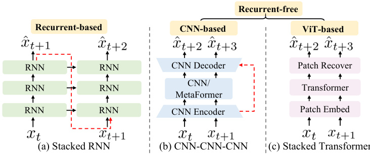
Figure 1. Main categories of video prediction framework. (a) Recurrent-based Framework (b) CNN Encoder-Decoder-based Recurrent-free Framework. (c) Pure transformer-based Recurrentfree Framework.
图 1: 视频预测框架的主要类别。(a) 基于循环的框架 (b) 基于CNN编码器-解码器的无循环框架。(c) 基于纯Transformer的无循环框架。
An intuitive solution directly adopts a pure transformer [32] structure, as it is an efficient alternative to RNNs and has better s cal ability than CNNs. Transformers have demonstrated remarkable success in visual tasks [1, 2, 6, 17, 31]. Previous video prediction methods try to combine Swin Transformer [17] in recurrent-based frameworks such as SwinLSTM [29] and integrate MetaFormer [41] as a temporal translator in recurrent-free CNN-based encoderdecoder frameworks such as OpenSTL [28]. Despite these advances, pure transformer-based architecture remains under explored mainly due to the challenges of capturing spatial and temporal relationships within a unified framework. While merging spatial and temporal dimensions and applying full attention is conceptually straightforward, it is computationally expensive because of the quadratic scaling of attention with sequence length. Several recent methods [1, 2, 31] decouple full attention and show that spatial and temporal relations can be treated separately in a factorized or interleaved manner to reduce complexity.
一种直观的解决方案是直接采用纯Transformer [32]结构,因其能高效替代RNN且比CNN具备更优的扩展性。Transformer在视觉任务中已展现出卓越成效 [1, 2, 6, 17, 31]。现有视频预测方法尝试将Swin Transformer [17] 整合到基于循环的框架(如SwinLSTM [29]),或将MetaFormer [41] 作为时序转换器集成到无循环的CNN编码器-解码器框架(如OpenSTL [28])。尽管取得进展,纯Transformer架构仍未被充分探索,主要源于在统一框架中捕获时空关系的挑战。虽然合并时空维度并应用全局注意力在概念上简单,但由于注意力机制随序列长度呈二次方增长,计算成本高昂。近期若干方法 [1, 2, 31] 通过解耦全局注意力,证明时空关系可通过因子化或交错方式分别处理以降低复杂度。
In this work, we propose PredFormer, a pure transformer-based architecture for video prediction. PredFormer dives into the decomposition of spatial and temporal transformers, integrating self-attention with gated linear units [5] to more effectively capture complex s patio temporal dynamics. In addition to retaining spatial-temporal full attention encoder and factorized encoder strategies for both spatial-first and temporal-first configurations, we introduce six novel interleaved s patio temporal transformer architectures, resulting in nine configurations. We explore how far this simple framework can go with different strategies of 3D Attention. This comprehensive investigation pushes the boundaries of current models and sets valuable benchmarks for spatial-temporal modeling.
在本工作中,我们提出了PredFormer,一种基于纯Transformer架构的视频预测方法。PredFormer深入探索了空间与时间Transformer的分解机制,通过将自注意力(self-attention)与门控线性单元[5]相结合,更有效地捕捉复杂的时空动态特性。除了保留时空全注意力编码器以及针对空间优先和时间优先配置的分解编码器策略外,我们引入了六种新颖的交错时空Transformer架构,最终形成九种配置方案。我们探究了这一简单框架在不同3D注意力策略下的性能极限。这项全面研究突破了现有模型的边界,为时空建模确立了有价值的基准。
Notably, PredFormer achieves state-of-the-art performance across four benchmark datasets, including synthetic prediction of moving objects, real-world human motion prediction, traffic flow prediction and weather forecasting, outperforming previous methods by a substantial margin without relying on complex model architectures or specialized loss functions.
值得注意的是,PredFormer在四个基准数据集上均实现了最先进的性能表现,涵盖移动物体合成预测、真实世界人体运动预测、交通流量预测和天气预报任务。其性能显著超越先前方法,且无需依赖复杂模型架构或专用损失函数。
The main contributions can be summarized as follows:
主要贡献可归纳如下:
2. Related Work
2. 相关工作
Recurrent-based video prediction. Recent advancements in recurrent-based video prediction models have integrated CNNs, ViTs, and Vision Mamba [16] into RNNs, employing various strategies to capture s patio temporal relationships. ConvLSTM [25], evolving from FC-LSTM [26], innovative ly integrates convolutional operations into the LSTM framework. PredNet [19] leverages deep recurrent convolutional neural networks with bottom-up and topdown connections to predict future video frames. PredRNN [34] introduces the S patio temporal LSTM (STLSTM) unit, which effectively captures and memorizes spatial and temporal representations by propagating hidden states horizontally and vertically. PredRNN $^{++}$ [35] incorporates a gradient highway unit and Causal LSTM to address the vanishing gradient problem and adaptively capture temporal dependencies. E3D-LSTM [36] extends the memory capabilities of ST-LSTM by integrating 3D convolutions. The MIM model [37] further refines the STLSTM by re imagining the forget gate with dual recurrent units and utilizing differential information between hidden states. CrevNet [40] employs a CNN-based reversible architecture to decode complex s patio temporal patterns. PredRNNv2 [38] enhances PredRNN by introducing a memory decoupling loss and a curriculum learning strategy. MAU [4] adds a motion-aware unit to capture dynamic motion information. SwinLSTM [29] integrates the Swin Transformer [17] module into the LSTM architecture, while VMRNN [30] extends this by incorporating the Vision Mamba module. Unlike these approaches, PredFormer is a recurrent-free method that offers superior efficiency.
基于循环网络的视频预测。近期基于循环网络的视频预测模型将CNN、ViT和Vision Mamba [16]整合到RNN中,采用多种策略捕捉时空关系。ConvLSTM [25]由FC-LSTM [26]演进而来,创新地将卷积运算融入LSTM框架。PredNet [19]利用具有自底向上和自顶向下连接的深度循环卷积神经网络预测未来视频帧。PredRNN [34]提出时空LSTM (STLSTM)单元,通过水平和垂直传播隐藏状态有效捕捉并记忆时空表征。PredRNN++ [35]引入梯度高速公路单元和因果LSTM,以解决梯度消失问题并自适应捕捉时间依赖性。E3D-LSTM [36]通过整合3D卷积扩展了ST-LSTM的记忆能力。MIM模型 [37]通过用双循环单元重构遗忘门并利用隐藏状态间的差分信息,进一步改进了STLSTM。CrevNet [40]采用基于CNN的可逆架构解码复杂时空模式。PredRNNv2 [38]通过引入记忆解耦损失和课程学习策略增强PredRNN。MAU [4]添加运动感知单元以捕捉动态运动信息。SwinLSTM [29]将Swin Transformer [17]模块集成到LSTM架构中,而VMRNN [30]则通过整合Vision Mamba模块扩展了这一方法。与这些方法不同,PredFormer是一种无循环结构的高效方案。
Recurrent-free video prediction. Recent recurrent-free models, e.g., SimVP [9], are developed based on a CNNbased encoder-decoder with a temporal translator. TAU [27] builds upon this by separating temporal attention into static intra-frame and dynamic inter-frame components, introducing a differential divergence loss to supervise interframe variations. OpenSTL [28] integrates a MetaFormer model as the temporal translator. Additionally, PhyDNet [10] incorporates physical principles into CNN architectures, while DMVFN [13] introduces a dynamic multiscale voxel flow network to enhance video prediction performance. Earth Former [8] presents a 2D CNN encoderdecoder architecture with cuboid attention.WAST [21] proposes a wavelet-based method, coupled with a waveletdomain High-Frequency Focal Loss. In contrast to prior methods, PredFormer advances video prediction with its recurrent-free, pure transformer-based architecture, leveraging a global receptive field to achieve superior performance, outperforming prior models without relying on complex architecture designs or specialized loss.
无循环视频预测。近期无循环模型如SimVP[9]基于CNN编码器-解码器架构并配备时序转换器开发。TAU[27]在此基础上将时序注意力分解为静态帧内与动态帧间组件,引入差分发散损失来监督帧间变化。OpenSTL[28]整合了MetaFormer模型作为时序转换器。PhyDNet[10]将物理原理融入CNN架构,DMVFN[13]则提出动态多尺度体素流网络以提升视频预测性能。EarthFormer[8]采用带立方体注意力的2D CNN编码器-解码器架构。WAST[21]提出基于小波变换的方法,配合小波域高频焦点损失。与现有方法不同,PredFormer通过无循环的纯Transformer架构推进视频预测,利用全局感受野实现卓越性能,无需依赖复杂架构设计或专用损失函数即超越先前模型。
Recurrent-based approaches struggle with parallel iz ation and performance, while CNN-based recurrent-free methods often sacrifice s cal ability and generalization despite their strong inductive biases. In contrast to prior methods, PredFormer advances video prediction with its recurrent-free, pure transformer-based architecture, leveraging a global receptive field to achieve superior performance, outperforming prior models without relying on complex model designs or specialized loss designs.
基于循环神经网络的方法难以实现并行化和性能提升,而基于CNN的无循环方法虽然具有强归纳偏置,却常常牺牲可扩展性和泛化能力。与先前方法不同,PredFormer采用无循环的纯Transformer架构推进视频预测任务,通过全局感受野实现卓越性能,在不依赖复杂模型设计或专用损失函数的情况下超越现有模型。
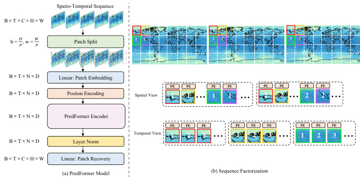
Figure 2. Overview of the PredFormer framework.
图 2: PredFormer框架概览
Vision Transformer (ViT). ViT [6] has demonstrated exceptional performance on various vision tasks. In video processing, TimeS former [2] investigates the factorization of spatial and temporal self-attention and proposes that divided attention where temporal and spatial attention are applied separately yields the best accuracy. ViViT [1] explores factorized encoders, self-attention, and dot product mechanisms, concluding that a factorized encoder with spatial attention applied first performs better. On the other hand, TSViT [31] finds that a factorized encoder prioritizing temporal attention achieves superior results. Latte [20] investigates factorized encoders and factorized self-attention mechanisms, incorporating both spatial-first and spatialtemporal parallel designs, within the context of latent diffusion transformers for video generation. Despite these advancements, most existing models focus primarily on video classification, with limited research on applying ViTs to spatio-temporal predictive learning. Moving beyond earlier methods that focus on factorizing self-attention, PredFormer explores the decomposition of spatial and temporal transformers at a deeper level by integrating self-attention with gated linear units and introducing innovative interleaved designs, allowing for a more robust capture of complex s patio temporal dynamics.
视觉Transformer (ViT)。ViT [6] 在各种视觉任务中展现出卓越性能。在视频处理领域,TimeSformer [2] 研究了空间与时间自注意力 (self-attention) 的分解机制,提出时序注意力与空间注意力分离应用的分治策略能获得最佳精度。ViViT [1] 探索了分解式编码器、自注意力机制和点积运算,发现优先应用空间注意力的分解编码器表现更优。而TSViT [31] 则证明优先时序注意力的分解编码器效果更佳。Latte [20] 在视频生成的潜在扩散Transformer框架下,同时研究了空间优先与时空并行的分解编码器及自注意力机制设计。尽管取得这些进展,现有模型仍主要聚焦视频分类任务,将ViT应用于时空预测学习的研究较为有限。与早期聚焦自注意力分解的方法不同,PredFormer 通过将自注意力与门控线性单元结合,并引入创新的交错式设计,在更深层次实现时空Transformer的分解,从而更稳健地捕捉复杂时空动态。
3. Method
3. 方法
To systematically analyze the transformer structure of the network model in spatial-temporal predictive learning, we propose the PredFormer as a general model design, as shown in Fig 2. In the following sections, we introduce the pure transformer-based architecture in Sec 3.1. Next, we describe the Gated Transformer Block (GTB) in Sec 3.2. Finally, we present how to use GTB to build a PredFormer layer and architecture variants in Sec 3.3.
为系统分析时空预测学习中网络模型的Transformer结构,我们提出了通用模型设计PredFormer,如图2所示。在后续章节中,我们将在3.1节介绍纯Transformer架构,在3.2节阐述门控Transformer块(GTB),最后在3.3节说明如何利用GTB构建PredFormer层及其架构变体。
3.1. Pure Transformer Based Architecture
3.1. 基于纯Transformer的架构
Patch Embedding. Follow the ViT design, PredFormer splits a sequence of frames $\mathcal{X}$ into a sequence of $N=$ $\left\lfloor{\frac{H}{p}}\right\rfloor\left\lfloor{\frac{W}{p}}\right\rfloor$ equally sized, non-overlapping patches of size $p$ , each of which is flattened into a 1D tokens. These tokens are then linearly projected into hidden dimensions $D$ and processed by a layer normalization (LN) layer, resulting in a tensor ′ RB×T ×N×D.
分块嵌入 (Patch Embedding)。遵循 ViT 设计,PredFormer 将帧序列 $\mathcal{X}$ 分割为 $N=$ $\left\lfloor{\frac{H}{p}}\right\rfloor\left\lfloor{\frac{W}{p}}\right\rfloor$ 个尺寸为 $p$ 的等大非重叠分块,每个分块被展平为 1D Token。这些 Token 随后通过线性投影映射到隐藏维度 $D$,并经过层归一化 (LN) 层处理,最终生成张量 ′ RB×T ×N×D。
Position Encoding. Unlike typical ViT approach, which employs learnable position embeddings, we incorporate a s patio temporal position encoding (PE) generated by sinusoidal functions with absolute coordinates for each patch.
位置编码 (Position Encoding)。与典型 ViT 方法使用可学习位置嵌入不同,我们采用由正弦函数生成的时空位置编码 (PE),为每个图像块分配绝对坐标。
PredFormer Encoder. The 1D tokens are then processed by a PredFormer Encoder for feature extraction. PredFormer Encoder is stacked by Gated Transformer Blocks in various manners.
PredFormer编码器。随后,一维Token会通过PredFormer编码器进行特征提取。PredFormer编码器由门控Transformer块以多种方式堆叠而成。
Patch Recovery. Since our encoder is based on a pure gated transformer, without convolution or resolution reduction, global context is modeled at every layer. This allows it to be paired with a simple decoder, forming a powerful prediction model. After the encoder, a linear layer serves as the decoder, projecting the hidden dimensions back to recover the 1D tokens to 2D patches.
补丁恢复。由于我们的编码器基于纯门控Transformer,不含卷积或分辨率降低操作,因此每一层都能建模全局上下文。这使得它可以与简单的解码器配对,形成强大的预测模型。在编码器之后,线性层作为解码器,将隐藏维度投影回原始空间,从而将一维Token恢复为二维补丁。
3.2. Gated Transformer Block
3.2. 门控Transformer模块
The Standard Transformer model [32] alternates between Multi-Head Attention (MSA) and Feed-Forward Networks (FFN). The attention mechanism for each head is defined as:
标准Transformer模型 [32] 在多头注意力机制 (MSA) 和前馈网络 (FFN) 之间交替进行。每个注意力头的计算机制定义为:
$$
{\mathrm{Attention}}(\mathbf{Q},\mathbf{K},\mathbf{V})={\mathrm{Softmax}}\left({\frac{\mathbf{Q}\mathbf{K}^{\top}}{\sqrt{d_{k}}}}\right)\mathbf{V},
$$
$$
{\mathrm{Attention}}(\mathbf{Q},\mathbf{K},\mathbf{V})={\mathrm{Softmax}}\left({\frac{\mathbf{Q}\mathbf{K}^{\top}}{\sqrt{d_{k}}}}\right)\mathbf{V},
$$
where in self-attention, the queries $\mathbf{Q}$ , keys $\mathbf{K}$ , and values $\mathbf{V}$ are linear projections of the input $\mathbf{X}$ , represented as $\mathbf{Q}=\mathbf{X}\mathbf{W}_{q}$ , $\mathbf{K}~=~\mathbf{X}\mathbf{W}_{k}$ , and $\mathbf{V}~=~\mathbf{X}\mathbf{W}_{v}$ , with ${\bf X},{\bf Q},{\bf K},{\bf V}\in\mathbb{R}^{N\times d}$ . The FFN then processes each position in the sequence by applying two linear transformations.
在自注意力机制中,查询 $\mathbf{Q}$ 、键 $\mathbf{K}$ 和值 $\mathbf{V}$ 是输入 $\mathbf{X}$ 的线性投影,表示为 $\mathbf{Q}=\mathbf{X}\mathbf{W}_{q}$ 、 $\mathbf{K}~=~\mathbf{X}\mathbf{W}_{k}$ 和 $\mathbf{V}~=~\mathbf{X}\mathbf{W}_{v}$ ,其中 ${\bf X},{\bf Q},{\bf K},{\bf V}\in\mathbb{R}^{N\times d}$ 。随后,前馈神经网络 (FFN) 通过应用两次线性变换处理序列中的每个位置。
Gated Linear Units (GLUs) [5], often used in place of simple linear transformations, involve the element-wise product of two linear projections, with one projection passing through a sigmoid function. Various GLU variants control the flow of information by substituting the sigmoid with other non-linear functions. For instance, SwiGLU [24] replaces the sigmoid with the Swish activation function (SiLU) [11], as shown in $\operatorname{Eq}2$ .
门控线性单元 (GLUs) [5] 通常用于替代简单的线性变换,它通过对两个线性投影进行逐元素乘积来实现,其中一个投影会经过sigmoid函数处理。不同的GLU变体通过用其他非线性函数替代sigmoid来控制信息流动。例如,SwiGLU [24] 使用Swish激活函数 (SiLU) [11] 替代sigmoid,如 $\operatorname{Eq}2$ 所示。
$$
\begin{array}{c}{{\operatorname{Swish}_{\beta}(x)=x\sigma(\beta x)}}\ {{\operatorname{SwiGLU}(x,W,V,b,c,\beta)=\operatorname{Swish}_{\beta}(x W+b)\otimes(x V+c)}}\end{array}
$$
$$
\begin{array}{c}{{\operatorname{Swish}_{\beta}(x)=x\sigma(\beta x)}}\ {{\operatorname{SwiGLU}(x,W,V,b,c,\beta)=\operatorname{Swish}_{\beta}(x W+b)\otimes(x V+c)}}\end{array}
$$
SwiGLU has been demonstrated to outperform Multi-layer Perce ptr on s (MLPs) in various natural language processing tasks[24]. Inspired by the SwiGLU’s success in these tasks, our Gated Transformer Block (GTB), incorporates MSA followed by a SwiGLU-based FFN, as illustrated in
SwiGLU 已被证明在各种自然语言处理任务中表现优于多层感知机 (MLP) [24]。受 SwiGLU 在这些任务中成功的启发,我们的门控 Transformer 模块 (GTB) 采用了多头自注意力机制 (MSA) 后接基于 SwiGLU 的前馈网络 (FFN),如图
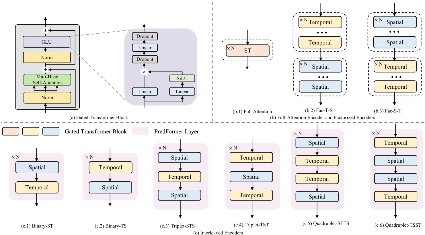
Figure 3. (a) Gated Transformer Block (b) Full Attention Encoder and Factorized Encoders (c) Interleaved Encoders with Binary, Triplet, and Quadrupled design
图 3: (a) 门控Transformer模块 (b) 全注意力编码器与因子化编码器 (c) 采用二元、三元及四元设计的交错编码器
Fig 3(a). GTB is defined as:
图 3(a): GTB 定义为:
$$
\begin{array}{c}{\mathbf{Y}^{l}=\mathbf{M}\mathbf{S}\mathbf{A}(\mathbf{L}\mathbf{N}(\mathbf{Z}^{l}))+\mathbf{Z}^{l}}\ {\mathbf{Z}^{l+1}=\mathbf{S}\mathrm{wiGLU}(\mathbf{L}\mathbf{N}(\mathbf{Y}^{l}))+\mathbf{Y}^{l}}\end{array}
$$
$$
\begin{array}{c}{\mathbf{Y}^{l}=\mathbf{M}\mathbf{S}\mathbf{A}(\mathbf{L}\mathbf{N}(\mathbf{Z}^{l}))+\mathbf{Z}^{l}}\ {\mathbf{Z}^{l+1}=\mathbf{S}\mathrm{wiGLU}(\mathbf{L}\mathbf{N}(\mathbf{Y}^{l}))+\mathbf{Y}^{l}}\end{array}
$$
3.3. Variants of PredFormer
3.3. PredFormer的变体
Modeling s patio temporal dependencies in video prediction is challenging, as the balance between spatial and temporal information differs significantly across tasks and datasets. Developing flexible and adaptive models that can accommodate varying dependencies and scales is thus critical. To address these, we explore both full-attention encoders and factorized encoders with spatial-first (Fac-S-T) and temporal-first (Fac-T-S) configurations, as shown in Fig 3(b). In addition, we introduce six interleaved models based on PredFormer layer, enabling dynamic interaction across multiple scales.
建模视频预测中的时空依赖性具有挑战性,因为空间与时间信息之间的平衡在不同任务和数据集间差异显著。因此,开发能够适应不同依赖关系和尺度的灵活自适应模型至关重要。为此,我们探索了全注意力编码器以及采用空间优先 (Fac-S-T) 和时间优先 (Fac-T-S) 配置的因子化编码器,如图 3(b) 所示。此外,我们基于 PredFormer 层引入了六种交错模型,实现跨多尺度的动态交互。
A PredFormer layer is a module capable of simultaneously processing spatial and temporal information. Building on this design principle, we propose three interleaved s patio temporal paradigms, Binary, Triplet, and Quadrupled, which sequentially model the relation from spatial and temporal views.
PredFormer层是一种能够同时处理空间和时间信息的模块。基于这一设计原则,我们提出了三种交错的空间-时间范式:二元(Binary)、三元(Triplet)和四元(Quadrupled),依次从空间和时间视角建模关系。
Ultimately, they yield six distinct architectural configurations. A detailed illustration of these nine variants is provided in Fig 3.
最终,他们得出了六种不同的架构配置。图3详细展示了这九种变体。
For full attention layers, given input X ∈ RB×T ×N×D, attention is computed over the sequence of length $T\times N$ . As illustrated in Fig 3 (b.1), we merge and flatten the spatial and temporal tokens to compute attention through several stacked $\mathrm{GTB}_{s t}$ .
对于全注意力层,给定输入X ∈ RB×T ×N×D,注意力计算在长度为$T\times N$的序列上进行。如图3 (b.1)所示,我们将空间和时序token合并并展平,通过多个堆叠的$\mathrm{GTB}_{st}$计算注意力。
For Binary layers, each GTB block processes temporal or spatial sequence independently, which we denote as a binary-TS or binary-ST layer. The input is first reshaped, and processed through $\mathbf{G}\mathbf{\dot{T}}\mathbf{B}{t}^{1}$ , where attention is applied over the temporal sequence. The tensor is then reshaped back to restore the temporal order. Subsequently, spatial attention is applied using another $\mathbf{GTB}_{s}^{2}$ , where the tensor is flattened along the temporal dimension and processed.
对于二元层 (Binary layers),每个GTB块独立处理时间或空间序列,我们分别称之为二元-TS层或二元-ST层。输入首先被重塑,并通过 $\mathbf{G}\mathbf{\dot{T}}\mathbf{B}{t}^{1}$ 进行处理,其中注意力机制应用于时间序列。随后张量被重塑回原始时序。接着使用另一个 $\mathbf{GTB}_{s}^{2}$ 应用空间注意力机制,此时张量沿时间维度展开并进行处理。
For Triplet and Quadruplet layers, additional blocks are stacked on top of the Binary structure. Triplet-TST captures more temporal dependencies, while Triplet-STS focuses more on spatial dependencies, both using the same number of parameters. The Quadruplet layer combines two Binary layers in different orders.
对于Triplet和Quadruplet层,会在Binary结构之上叠加额外的模块。Triplet-TST通过相同参数量捕获更多时间依赖性,而Triplet-STS则更侧重空间依赖性。Quadruplet层通过不同顺序组合两个Binary层实现功能拓展。
4. Experiments
4. 实验
We present extensive evaluations of PredFormer and stateof-the-art methods. We conduct experiments across synthetic and real-world scenarios, including long-term prediction(moving object trajectory prediction and weather forecasting), and short-term prediction(traffic flow prediction and human motion prediction). The statistics of the data set are presented in the Tab 1. These datasets have different spatial resolutions, temporal frames, and intervals, which determine their different s patio temporal dependencies.
我们对PredFormer和最先进方法进行了广泛评估。实验涵盖合成场景和真实场景,包括长期预测(移动物体轨迹预测和天气预报)和短期预测(交通流量预测和人体运动预测)。数据集统计信息如 表1 所示。这些数据集具有不同的空间分辨率、时间帧和间隔,这决定了它们不同的时空依赖性。
Table 1. Benchmark datasets for PredFormer.
表 1: PredFormer的基准数据集
| 数据集 | 训练集大小 | 测试集大小 | 通道数 | 高度 | 宽度 | TT'I | 间隔 |
|---|---|---|---|---|---|---|---|
| MovingMNIST | 10,000 | 10,000 | 1 | 64 | 64 | 1010 | |
| Human3.6m | 73404 | 8582 | 3 | 256 | 256 | 44 frame | |
| WeatherBench-S | 52559 | 17495 | 1 | 32 | 64 | 121230min | |
| TaxiBJ | 20,461 | 500 | 2 | 32 | 32 | 441hour |
Implementation Details Our method is implemented in PyTorch. The experiments are conducted on a single 24GB NVIDIA RTX 3090.
实现细节
我们的方法基于 PyTorch 实现,实验在单张 24GB NVIDIA RTX 3090 显卡上完成。
PredFormer is optimized using the AdamW [18] optimizer with an L2 loss, a weight decay of 1e-2, and a learning rate selected from ${5\mathrm{e}{-}4,1\mathrm{e}{-}3}$ for best performance. OneCycle scheduler is used for Moving MNIST and TaxiBJ, while the Cosine scheduler is applied for Human3.6m and Weather Bench. Dropout [12] and stochastic depth [14] regular iz ation prevent over fitting. Further hyper parameter details are provided in the Appendix. For different PredFormer variants, we maintain a constant number of GTB blocks to ensure comparable parameters. In cases where the Triplet model cannot be evenly divided, we use the number of GTB blocks closest to the others.
PredFormer 使用 AdamW [18] 优化器进行优化,采用 L2 损失函数,权重衰减为 1e-2,学习率从 ${5\mathrm{e}{-}4,1\mathrm{e}{-}3}$ 中选择以获得最佳性能。Moving MNIST 和 TaxiBJ 数据集使用 OneCycle 调度器,而 Human3.6m 和 Weather Bench 数据集采用 Cosine 调度器。通过 Dropout [12] 和随机深度 (stochastic depth) [14] 正则化防止过拟合。更多超参数细节见附录。对于不同 PredFormer 变体,我们保持 GTB 块数量恒定以确保参数可比性。若 Triplet 模型无法均分,则使用最接近其他模型的 GTB 块数量。
Evaluation Metrics We assess model performance using a suite of metrics. (1) Pixel-wise error is measured using Mean Squared Error (MSE), Mean Absolute Error (MAE), and Root Mean Squared Error (RMSE). (2) Predicted frame quality is evaluated using the structural similarity index measure (SSIM) metric [39]. Lower MSE, MAE, and RMSE values, combined with higher SSIM, signify better predictions. (3) Computational efficiency is assessed by the number of parameters, floating-point operations (FLOPs), and inference speed in frames per second (FPS) on a NVIDIA A6000 GPU. This evaluation framework comprehensively evaluates accuracy and efficiency.
评估指标
我们使用一组指标评估模型性能。(1) 像素级误差通过均方误差 (MSE)、平均绝对误差 (MAE) 和均方根误差 (RMSE) 衡量。(2) 预测帧质量采用结构相似性指数 (SSIM) [39] 进行评估。更低的 MSE、MAE 和 RMSE 值结合更高的 SSIM 值代表更优的预测效果。(3) 计算效率通过参数量、浮点运算量 (FLOPs) 及在 NVIDIA A6000 GPU 上的每秒推理帧数 (FPS) 进行评估。该评估框架全面衡量了准确性与效率。
4.1. Synthetic Moving Object Prediction
4.1. 合成移动物体预测
Moving MNIST. The moving MNIST dataset [26] serves as a benchmark synthetic dataset for evaluating sequence reconstruction models. We follow [26] to generate Moving MNIST sequences with 20 frames, using the initial 10 frames for input and the subsequent 10 frames as the prediction target. We adopt 10000 sequences for training, and for fair comparisons, we use the pre-generated 10000 sequences [9] for validation.
移动MNIST。移动MNIST数据集 [26] 是用于评估序列重建模型的基准合成数据集。我们按照 [26] 的方法生成包含20帧的移动MNIST序列,其中前10帧作为输入,后10帧作为预测目标。训练集采用10000个序列,为公平比较,验证集使用预生成的10000个序列 [9]。
On the Moving MNIST dataset, following prior work [9, 27], we train our models for 2000 epochs and report our results in Tab 2. We train OpenSTL methods with ViT and Swin Transformer as temporal translators for 2000 epochs as recurrent-free baselines. We cite other results from each original paper for a fair comparison.
在Moving MNIST数据集上,遵循先前工作[9,27],我们将模型训练2000个周期并在表2中报告结果。我们使用ViT和Swin Transformer作为时序转换器训练OpenSTL方法2000个周期,作为无循环基线。为公平比较,其他结果引自各原始论文。
Table 2. Quantitative comparison on Moving MNIST. Each model observes 10 frames and predicts the subsequent 10 frames. We highlight the best experimental results in bold red and the second-best in blue.
表 2: Moving MNIST定量对比。各模型观测10帧并预测后续10帧。最优实验结果用红色加粗标出,次优结果用蓝色标出。
| 方法 | 参数量(M) | 计算量(G) | 帧率(FPS) | MSE↓ | MAE↓ | SSIM↑ |
|---|---|---|---|---|---|---|
| ConvLSTM | 15.0 | 56.8 | 113 | 103.3 | 182.9 | 0.707 |
| PredRNN | 23.8 | 116.0 | 54 | 56.8 | 126.1 | 0.867 |
| PredRNN++ | 38.6 | 171.7 | 38 | 46.5 | 106.8 | 0.898 |
| MIM | 38.0 | 179.2 | 37 | 44.2 | 101.1 | 0.910 |
| E3D-LSTM | 51.0 | 298.9 | 18 | 41.3 | 86.4 | 0.910 |
| PhyDNet | 3.1 | 15.3 | 182 | 24.4 | 70.3 | 0.947 |
| MAU | 4.5 | 17.8 | 201 | 27.6 | 86.5 | 0.937 |
| PredRNNv2 | 24.6 | 708.0 | 24 | 48.4 | 129.8 | 0.891 |
| SwinLSTM | 20.2 | 69.9 | 62 | 17.7 | - | 0.962 |
| SimVP | 58.0 | 19.4 | 209 | 23.8 | 68.9 | 0.948 |
| TAU | 44.7 | 16.0 | 283 | 19.8 | 60.3 | 0.957 |
| OpenSTL_ViT | 46.1 | 16.9 | 290 | 19.0 | 60.8 | 0.955 |
| OpenSTL_Swin | 46.1 | 16.9 | 290 | 18.3 | 59.0 | 0.960 |
| PredFormer | - | - | - | - | - | - |
| Full Attention | 25.3 | 21.2 | 254 | 17.3 | 56.0 | 0.962 |
| Fac-S-T | 25.3 | 16.5 | 368 | 20.6 | 63.5 | 0.955 |
| Fac-T-S | 25.3 | 16.5 | 370 | 16.9 | 55.8 | - |
| Binary-TS | 25.3 | 16.5 | - | - | - | 0.963 |
| Binary-ST | 25.3 | - | 301 | 12.8 | 46.1 | 0.972 |
| Triplet-TST | 25.3 | 16.5/16.4 | 316/312 | 13.4 | 47.1 | 0.971 |
| Triplet-STS | 25.3 | 16.5 | 321 | 13.1 | 46.7 | 0.972 |
| Quadruplet-TSST | 25.3 | 16.5 | 302 | 12.4 | 44.6 | 0.973 |
| Quadruplet-STTS | 25.3 | 16.4 | 322 | 12.4 | 44.9 | 0.973 |
Compared to $\mathrm{{SimVP}}$ PredFormer achieves substantial performance gains while maintaining a lightweight structure. Specifically, it reduces MSE by $48%$ (from 23.8 to 12.4), significantly improving prediction accuracy. Meanwhile, PredFormer requires far fewer parameters (25.3M vs. $58.0\mathbf{M}$ in $\mathrm{SimVP}$ ) and operates with lower FLOPs (16.5G vs. 19.4G), showcasing its superior efficiency.
与 $\mathrm{{SimVP}}$ 相比,PredFormer 在保持轻量级结构的同时实现了显著的性能提升。具体而言,它将 MSE (均方误差) 降低了 $48%$ (从 23.8 降至 12.4),显著提高了预测精度。与此同时,PredFormer 所需的参数量更少 (25.3M vs. $\mathrm{SimVP}$ 的 $58.0\mathbf{M}$),且运算量更低 (16.5G vs. 19.4G FLOPs),展现了其卓越的效率。
Notably, even when $\operatorname{SimVP}$ incorporates ViT and Swin Transformer as the temporal translator, its performance remains far below that of PredFormer. This is because, while $\operatorname{SimVP}$ benefits from the inductive bias of using CNNs as the encoder and decoder, this design inherently limits the model’s performance ceiling. In contrast, PredFormer effectively models global s patio temporal dependencies, allowing it to surpass these constraints and achieve superior predictive accuracy.
值得注意的是,即使当 $\operatorname{SimVP}$ 采用 ViT 和 Swin Transformer 作为时序翻译器时,其性能仍远低于 PredFormer。这是因为,虽然 $\operatorname{SimVP}$ 受益于使用 CNN 作为编码器和解码器的归纳偏置,但这种设计本质上限制了模型的性能上限。相比之下,PredFormer 能有效建模全局时空依赖性,从而突破这些限制并实现更优的预测精度。
Compared to SwinLSTM, PredFormer achieves higher accuracy. Although SwinLSTM outperforms SimVP in terms of MSE (17.7 vs. 23.8), its reliance on an RNN-based structure results in significantly higher computational cost. SwinLSTM exhibits high FLOPs (69.9G) and lower FPS, making it less efficient for large-scale deployment. This highlights the limitations of recurrent structures in video prediction, whereas PredFormer, with its recurrence-free transformer framework, achieves both higher accuracy and superior efficiency.
与SwinLSTM相比,PredFormer实现了更高的精度。尽管SwinLSTM在MSE指标上优于SimVP (17.7 vs. 23.8),但其基于RNN的结构导致计算成本显著增加。SwinLSTM具有较高的FLOPs (69.9G)和较低的FPS,使其在大规模部署时效率较低。这凸显了循环结构在视频预测中的局限性,而采用无循环Transformer架构的PredFormer同时实现了更高精度和更优效率。
Among the PredFormer variants, Quadruplet-TSST achieves the best MSE of 12.4, followed closely by Quadruplet-STTS. These results highlight PredFormer’s ability to fully leverage global information fully, further validating its effectiveness in video prediction.
在PredFormer的变体中,Quadruplet-TSST以12.4的MSE取得了最佳表现,紧随其后的是Quadruplet-STTS。这些结果凸显了PredFormer充分利用全局信息的能力,进一步验证了其在视频预测中的有效性。
Table 3. Quantitative comparison on Human3.6m. Each model observes 4 frames and predicts the subsequent 4 frames.
For * models, we add a skip connection for each PredFormer Layer for stable training.
表 3. Human3.6m数据集上的定量比较。各模型观察4帧并预测后续4帧。
| 方法 | 参数量(M) | 计算量(G) | FPS | MSE← | MAE↓ | SSIM↑ | PSNR↑ | LPIPS↓ |
|---|---|---|---|---|---|---|---|---|
| ConvLSTM | 15.5 | 347.0 | 52 | 125.5 | 1566.7 | 0.9813 | 33.40 | 0.03557 |
| PredNet | 12.5 | 13.7 | 176 | 261.9 | 1625.3 | 0.9786 | 31.76 | 0.03264 |
| PredRNN | 24.6 | 704.0 | 25 | 113.2 | 1458.3 | 0.9831 | 33.94 | 0.03245 |
| PredRNN++ | 39.3 | 1033.0 | 18 | 110.0 | 1452.2 | 0.9832 | 34.02 | 0.03196 |
| MIM | 47.6 | 1051.0 | 17 | 112.1 | 1467.1 | 0.9829 | 33.97 | 0.03338 |
| E3D-LSTM | 60.9 | 542.0 | 7 | 143.3 | 1442.5 | 0.9803 | 32.52 | 0.04133 |
| PhyDNet | 4.2 | 19.1 | 57 | 125.7 | 1614.7 | 0.9804 | 33.05 | 0.03709 |
| MAU | 20.2 | 105.0 | 6 | 127.3 | 1577.0 | 0.9812 | 33.33 | 0.03561 |
| PredRNNv2 | 24.6 | 708.0 | 24 | 114.9 | 1484.7 | 0.9827 | 33.84 | 0.03334 |
| SimVP | 41.2 | 197.0 | 26 | 115.8 | 1511.5 | 0.9822 | 33.73 | 0.03467 |
| TAU | 37.6 | 182.0 | 26 | 113.3 | 1390.7 | 0.9839 | 34.03 | 0.02783 |
| OpenSTL_ViT | 28.3 | 239.0 | 17 | 136.3 | 1603.5 | 0.9796 | 33.10 | 0.03729 |
| OpenSTL_Swin | 38.8 | 188.0 | 28 | 133.2 | 1599.7 | 0.9799 | 33.16 | 0.03766 |
| PredFormer | - | - | - | - | - | - | - | - |
| Full Attention | 12.7 | 155.0 | 16 | 113.9 | 1412.4 | 0.9833 | 33.98 | 0.03279 |
| Fac-S-T | 12.7 | 65.0 | 76 | 153.4 | 1630.7 | 0.9784 | 32.30 | 0.04676 |
| Fac-T-S | 12.7 | 65.0 | 75 | 118.4 | 1504.7 | 0.9820 | 33.67 | 0.03284 |
| Binary-TS | 12.7 | 65.0 | 75 | 111.2 | 1380.4 | 0.9838 | 34.13 | 0.03008 |
| Binary-ST | 12.7 | 65.0 | 78 | 112.7 | 1386.3 | 0.9836 | 34.07 | 0.03017 |
| Triplet-TST* | 12.7 | 60.8 | 88 | 112.4 | 1406.2 | 0.9834 | 34.05 | 0.02748 |
| Triplet-STS* | 12.7 | 69.3 | 64 | 111.8 | 1410.3 | 0.9834 | 34.07 | 0.02933 |
| Quadruplet-TSST | 12.7 | 65.0 | 72 | 110.9 | 1380.3 | 0.9839 | 34.14 | 0.03069 |
| Quadruplet-STTS | 12.7 | 65.0 | 74 | 113.4 | 1405.7 | 0.9835 | 34.04 | 0.02918 |
标有*的模型在每层PredFormer中增加了跳跃连接以稳定训练。
4.2. Real-world Human Motion Prediction
4.2. 真实世界人体运动预测
Human3.6m. The Human3.6M dataset [15] comprises 3.6 million unique human poses with their corresponding images, serving as a benchmark for motion prediction tasks. Human motion prediction is particularly challenging due to high resolution input and complex human movement dynamics. Following OpenSTL [28], we downsample the dataset from $1000{\times}1000{\times}3$ to $256\times256\times3$ . We use four observations to predict the next four frames.
Human3.6m。Human3.6M数据集 [15] 包含360万组独特人体姿态及其对应图像,是运动预测任务的基准数据集。由于高分辨率输入和复杂人体运动动力学特性,人体运动预测具有显著挑战性。依照OpenSTL [28] 的方法,我们将数据集从 $1000{\times}1000{\times}3$ 下采样至 $256\times256\times3$ ,使用四帧观察数据来预测后续四帧。
Compared to $\mathrm{{SimVP},}$ PredFormer Quadruplet-TSST reduces MSE from 115.8 to 110.9, significantly improving human motion prediction. At the same time, PredFormer requires only $12.7\mathbf{M}$ parameters, much fewer than SimVP’s $41.2\mathbf{M}$ . Furthermore, its computational cost is only 65G FLOPs, less than one third of SimVP’s 197G, while maintaining a higher inference speed.
与 $\mathrm{{SimVP},}$ 相比,PredFormer Quadruplet-TSST 将 MSE 从 115.8 降至 110.9,显著提升了人体运动预测性能。同时,PredFormer 仅需 $12.7\mathbf{M}$ 参数量,远低于 SimVP 的 $41.2\mathbf{M}$。此外,其计算成本仅为 65G FLOPs,不到 SimVP 197G 的三分之一,同时保持了更高的推理速度。
PredFormer also substantially reduces the computational cost compared to PredRNN $^{++}$ . While PredRNN $++$ requires 1033G FLOPs, PredFormer Quadruplet-TSST achieves comparative MSE and superior MAE and SSIM using only one-tenth of the computation.
PredFormer 相比 PredRNN$^{++}$ 还大幅降低了计算成本。PredRNN$^{++}$ 需要 1033G FLOPs,而 PredFormer Quadruplet-TSST 仅用十分之一的计算量就达到了相当的 MSE (均方误差) 和更优的 MAE (平均绝对误差) 与 SSIM (结构相似性指数)。
Compared to OpenSTL-ViT and OpenSTL-Swin Transformer, which rely on ViT-based architectures but struggle with prediction accuracy, PredFormer utilizes the Transformer structures more effectively for video prediction. OpenSTL-ViT and OpenSTL-Swin both perform worse than $\mathrm{{SimVP},}$ indicating that simply applying Transformers does not guarantee strong results. In contrast, PredFormer outperforms them while maintaining an efficient design, demonstrating its capability in s patio temporal modeling.
与依赖基于ViT架构但在预测精度上表现不佳的OpenSTL-ViT和OpenSTL-Swin Transformer相比,PredFormer更有效地利用了Transformer结构进行视频预测。OpenSTL-ViT和OpenSTL-Swin的表现均逊于$\mathrm{{SimVP},}$,这表明简单地应用Transformer并不能保证获得强劲的结果。相比之下,PredFormer在保持高效设计的同时表现更优,展现了其在时空建模方面的能力。
Table 4. Quantitative comparison on TaxiBJ. Each model observes 4 frames and predicts the subsequent 4 frames.
表 4. TaxiBJ数据集上的量化对比。各模型观测4帧并预测后续4帧。
| 方法 | 参数量(M) | 计算量(G) | FPS | MSE↓ | MAE↓ | SSIM↑ |
|---|---|---|---|---|---|---|
| ConvLSTM | 15.0 | 20.7 | 815 | 0.485 | 17.7 | 0.978 |
| PredRNN | 23.7 | 42.4 | 416 | 0.464 | 16.9 | 0.977 |
| PredRNN++ | 38.4 | 63.0 | 301 | 0.448 | 16.9 | 0.971 |
| MIM | 37.9 | 64.1 | 275 | 0.429 | 16.6 | 0.971 |
| E3D-LSTM | 51.0 | 98.2 | 60 | 0.432 | 16.9 | 0.979 |
| PhyDNet | 3.1 | 5.6 | 982 | 0.362 | 15.5 | 0.983 |
| PredRNNv2 | 23.7 | 42.6 | 378 | 0.383 | 15.5 | 0.983 |
| SwinLSTM | 2.9 | 1.3 | 1425 | 0.303 | 15.0 | 0.984 |
| SimVP | 13.8 | 3.6 | 533 | 0.414 | 16.2 | 0.982 |
| TAU | 9.6 | 2.5 | 1268 | 0.344 | 15.6 | 0.983 |
| OpenSTL_ViT | 9.7 | 2.8 | 1301 | 0.317 | 15.2 | 0.984 |
| OpenSTL_Swin | 9.7 | 2.6 | 1506 | 0.313 | 15.1 | 0.985 |
| PredFormer | - | - | - | - | - | - |
| Full Attention | 8.4 | 2.4 | 2438 | 0.316 | 14.6 | 0.985 |
| Fac-S-T | 8.4 | 2.2 | 3262 | 0.320 | 15.2 | 0.984 |
| Fac-T-S | 8.4 | 2.2 | 3224 | 0.283 | 14.4 | 0.985 |
| Binary-TS | 8.4 | 2.2 | 3192 | 0.286 | 14.6 | 0.985 |
| Binary-ST | 8.4 | 2.2 | 3172 | 0.277 | 14.3 | 0.986 |
| Triplet-TST | 6.3 | 1.6 | 4348 | 0.293 | 14.7 | 0.985 |
| Triplet-STS | 6.3 | 1.6 | 4249 | 0.277 | 14.3 | 0.986 |
| Quadruplet-TSST | 8.4 | 2.2 | 3230 | 0.284 | 14.4 | 0.986 |
| Quadruplet-STTS | 8.4 | 2.2 | 3259 | 0.293 | 14.6 | 0.985 |
4.3. Traffic Flow Prediction
4.3. 交通流量预测
TaxiBJ. TaxiBJ [42] includes GPS data from taxis and mete oro logical data in Beijing. Each data frame is visualized as a $32\times32\times2$ heatmap, where the third dimension encapsulates the inflow and outflow of traffic within a designated area. Following previous work [42], we allocate the final four weeks’ data for testing, utilizing the preceding data for training. Our prediction model uses four sequential observations to forecast the subsequent four frames.
TaxiBJ
TaxiBJ [42] 包含北京出租车GPS数据和气象数据。每个数据帧可视化为一个 $32\times32\times2$ 热力图,其中第三维度表示指定区域内的交通流入量和流出量。遵循先前工作 [42],我们分配最后四周数据进行测试,并使用之前的数据进行训练。我们的预测模型使用四个连续观测值来预测后续四个帧。
Compared to SimVP, PredFormer significantly improves the accuracy of the prediction, reducing the MSE from 0.414 to 0.277 $(33%)$ while using fewer parameters (8.4M vs 13.8M) and a lower computational cost (2.2G FLOPs vs. 3.6G FLOPs). Despite this efficiency, PredFormer also dramatically increases inference speed, with FPS rising from 533 in $\operatorname{SimVP}$ to 4249.
与SimVP相比,PredFormer显著提升了预测精度,将MSE从0.414降至0.277 $(33%)$,同时使用更少的参数(8.4M vs 13.8M)和更低的计算成本(2.2G FLOPs vs. 3.6G FLOPs)。尽管效率更高,PredFormer还大幅提升了推理速度,FPS从 $\operatorname{SimVP}$ 的533提升至4249。
Furthermore, OpenSTL-ViT and OpenSTL-Swin, which adopt ViT-based architectures as temporal translators, achieve MSEs of 0.317 and 0.313, both worse than PredFormer’s best results. This suggests that using CNNs for the encoder and decoder provides strong inductive bias but inherently limits the model’s performance ceiling. Among the variants of PredFormer, Binary-ST and Triplet-STS achieve the best MSE of 0.277.
此外,采用基于ViT架构作为时间转换器的OpenSTL-ViT和OpenSTL-Swin分别取得了0.317和0.313的MSE值,均逊于PredFormer的最佳结果。这表明使用CNN作为编码器和解码器虽能提供强归纳偏置,但本质上限制了模型的性能上限。在PredFormer的变体中,Binary-ST和Triplet-STS以0.277的MSE达到了最优表现。
Table 5. Quantitative comparison on Weather Bench(T2m). Each model observes 12 frames and predicts the subsequent 12 frames.
表 5. Weather Bench(T2m)定量比较。各模型观测12帧并预测后续12帧。
| 方法 | 参数量(M) | 计算量(G) | 帧率(FPS) | MSE↓ | MAE↓ | SSIM↑ |
|---|---|---|---|---|---|---|
| ConvLSTM | 14.9 | 136.0 | 46 | 1.521 | 0.7949 | 1.233 |
| PredRNN | 23.6 | 278.0 | 22 | 1.331 | 0.7246 | 1.154 |
| PredRNN++ | 38.3 | 413 | 15 | 1.634 | 0.7883 | 1.278 |
| MIM | 37.8 | 109.0 | 126 | 1.784 | 0.8716 | 1.336 |
| PhyDNet | 3.1 | 36.8 | 177 | 285.9 | 8.7370 | 16.91 |
| MAU | 5.5 | 39.6 | 237 | 1.251 | 0.7036 | 1.119 |
| PredRNNv2 | 23.6 | 279.0 | 22 | 1.545 | 0.7986 | 1.243 |
| SimVP | 14.8 | 8.0 | 196 | 1.238 | 0.7037 | 1.113 |
| TAU | 12.2 | 6.7 | 229 | 1.162 | 0.6707 | 1.078 |
| OpenSTL_ViT | 12.4 | 8.0 | 432 | 1.146 | 0.6712 | 1.070 |
| OpenSTL_Swin | 12.4 | 6.9 | 581 | 1.143 | 0.6735 | 1.069 |
| PredFormer | - | - | - | - | - | - |
| Full Attention | 5.3 | 17.8 | 177 | 1.126 | 0.6540 | 1.061 |
| Fac-S-T | 5.3 | 8.5 | 888 | 1.783 | 0.8688 | - |
| Fac-T-S | 5.3 | 8.5 | 860 | 1.100 | 0.6469 | 1.335 |
| Binary-TS | 5.3 | 8.6 | 837 | 1.115 | 0.6508 | 1.049 |
| Binary-ST | 5.3 | 8.6 | 847 | 1.140 | 0.6571 | 1.056 |
| Triplet-TST | 4.0 | 6.3 | 1064 | 1.108 | 0.6492 | 1.068 |
| Triplet-STS | 4.0 | 6.5 | 1001 | 1.149 | - | 1.053 |
| - | - | - | 802 | 1.116 | 0.6658 | 1.072 |
| Quadruplet-TSST | 5.3 | 8.6 | - | - | 0.6510 | 1.057 |
| Quadruplet-STTS | 5.3 | 8.6 | 858 | 1.118 | 0.6507 | 1.057 |
4.4. Weather Forecasting
4.4. 天气预报
Weather Bench. Climate prediction is a critical challenge in s patio temporal predictive learning. The WeatherBench [23] dataset provides a comprehensive global weather forecasting resource, covering various climatic factors. In our experiments, we utilize Weather Bench-S, a single-variable setup where each climatic factor is trained independently. We focus on temperature prediction at a $5.625^{\circ}$ resolution ( $32\times64$ grid points). The model is trained on data spanning 2010-2015, validated on data from 2016, and tested on data from 2017-2018, all with a one-hour temporal interval. We input the first 12 frames and predict the subsequent 12 frames in this setting.
Weather Bench。气候预测是时空预测学习中的关键挑战。WeatherBench [23] 数据集提供了全面的全球天气预报资源,涵盖多种气候因子。在我们的实验中,我们使用 Weather Bench-S 单变量设置,其中每个气候因子独立训练。我们专注于 $5.625^{\circ}$ 分辨率 ( $32\times64$ 网格点) 下的温度预测。模型在 2010-2015 年的数据上训练,在 2016 年的数据上验证,并在 2017-2018 年的数据上测试,所有数据时间间隔为一小时。在此设置下,我们输入前 12 帧并预测后续 12 帧。
On Weather Bench $(\mathrm{T}2\mathrm{m})$ , RNN-based models like ConvLSTM and PredRNN have high computational costs but poor performance. PredRNN and PredRNNv2 reach 278.0G and 279.0G FLOPs, yet their MSE remains at 1.331 and 1.545, respectively, highlighting the inefficiency of RNN structures for this task.
在Weather Bench $(\mathrm{T}2\mathrm{m})$ 任务上,基于RNN的模型如ConvLSTM和PredRNN计算成本高但性能不佳。PredRNN和PredRNNv2分别达到278.0G和279.0G FLOPs,而它们的MSE仍停留在1.331和1.545,凸显了RNN结构对此任务的低效性。
$\operatorname{SimVP}$ reduces parameter count to half of PredRNN, lowers FLOPs to 8.0G, and achieves an improved MSE of 1.238, making it more efficient than RNN models. PredFormer further improves performance, using only half the parameters of SimVP while maintaining similar or lower FLOPs, achieving the best MSE of 1.100. The Fac-T-S and Triplet-TST variants deliver the top results. It also demonstrates a significant FPS advantage, with Binary-TS and Triplet-TST achieving 837 and 1064 FPS, respectively, compared to SimVP’s 196, highlighting the model’s superior efficiency in both computation and prediction speed.
$\operatorname{SimVP}$ 将参数量减少至PredRNN的一半,FLOPs降至8.0G,并将MSE提升至1.238,效率优于RNN模型。PredFormer进一步优化性能,仅使用SimVP一半的参数量,在保持相近或更低FLOPs的同时,取得了1.100的最佳MSE。其中Fac-T-S和Triplet-TST变体表现最为突出。该模型还展现出显著的FPS优势,Binary-TS和Triplet-TST分别达到837和1064 FPS,远超SimVP的196 FPS,凸显了其在计算效率和预测速度上的双重优越性。
Table 6. Ablation on PredFormer Layer Number on Moving MNIST.
表 6. PredFormer 层数在 Moving MNIST 上的消融实验
| TSSTLayer | Paras(M) | Flops(G) | FPS | MSE√N | MAE√S | SSIM↑ |
|---|---|---|---|---|---|---|
| 2 | 8.5 | 5.5 | 887 | 20.1 | 65.2 | 0.955 |
| 3 | 12.7 | 8.3 | 621 | 16.2 | 55.1 | 0.965 |
| 4 | 16.9 | 11.0 | 457 | 13.5 | 47.9 | 0.970 |
| 5 | 21.1 | 13.7 | 376 | 12.7 | 45.5 | 0.972 |
| 6 | 25.3 | 16.5 | 302 | 12.4 | 44.6 | 0.973 |
| 7 | 29.5 | 19.2 | 277 | 12.3 | 44.2 | 0.973 |
| 8 | 33.7 | 22.0 | 240 | 11.7 | 41.8 | 0.975 |
Table 7. Ablation on Gate Linear Unit and Position Encoding.
表 7: 门控线性单元与位置编码的消融实验
| 模型 | WeatherBench(T2m) MSE√MAE√RMSE√ | TaxiBJ MSE←MAE↓ |
|---|---|---|
| PredFormer | 1.100 | 0.6489 |
| SwiGLU→MLP | 1.171 | 0.6707 |
| PE:Abs→Learnable | 1.164 | 0.6771 |
Table 8. Ablation on Dropout and Stochastic Depth.
表 8: Dropout与随机深度的消融实验
| WeatherBench(T2m) | TaxiBJ | ||
|---|---|---|---|
| Model DP+UniSD | MSE√MAE↓RMSE√ 1.100 | 1.049 | MSE√MAE↓ 0.277 14.3 |
| 0.6489 | 15.1 | ||
| W/oReg + DP | 1.244 0.7057 1.210 0.6887 | 1.115 1.100 | 0.319 0.283 |
| + Uni SD | 1.156 0.6573 | 1.075 | 14.5 0.288 14.6 |
| +DP+LinearSD | 1.138 0.6533 | 1.067 | 0.299 14.8 |
4.5. Ablation Study and Discussion
4.5. 消融研究与讨论
PredFormer Layer Number. We conduct an ablation study on the number of TSST layers in PredFormer to evaluate its s cal ability and potential for performance improvement, as shown in Tab 6. The results show that as the number of layers increases, PredFormer continues to achieve better results, surpassing the 6-layer TSST configuration reported in Tab 2. With 2 TSST layers, PredFormer already outperforms SimVP, achieving a lower MSE of 20.1 while maintaining high efficiency. When increasing to 3 layers, PredFormer surpasses TAU, OpenSTL-ViT, and OpenSTL-Swin, achieving a lower MSE of 16.2 while requiring only half the FLOPs of these models and delivering twice their FPS. With 8 layers, PredFormer achieves an MSE of 11.7, which represents a $51%$ MSE reduction compared to SimVP. This substantial improvement demonstrates the s cal ability of PredFormer.
PredFormer层数研究。我们对PredFormer中TSST层数进行消融实验,以评估其扩展能力和性能提升潜力,如表6所示。结果表明随着层数增加,PredFormer持续取得更优结果,超越了表2中报告的6层TSST配置。当采用2层TSST时,PredFormer已优于SimVP,在保持高效的同时实现20.1的更低MSE。增至3层时,PredFormer超越了TAU、OpenSTL-ViT和OpenSTL-Swin,仅需这些模型一半的FLOPs便实现16.2的更低MSE,并提供两倍的FPS。当层数达到8层时,PredFormer取得11.7的MSE,较SimVP实现51%的MSE降低。这一显著改进证明了PredFormer的扩展能力。
We conduct ablation studies on our PredFormer model design and summarize the results in Tab 7 and Tab 8. We choose the best Triplet-STS model on TaxiBJ, and the best Fac-T-S model on Weather Bench as baselines.
我们对PredFormer模型设计进行了消融研究,并将结果总结在表7和表8中。在TaxiBJ数据集上选择最佳Triplet-STS模型,在Weather Bench数据集上选择最佳Fac-T-S模型作为基线。
Gate Linear Unit. Replacing SwiGLU with a standard MLP results in a notable performance degradation. On TaxiBJ, the MSE rises from 0.277 to 0.306, and on WeatherBench from 1.100 to 1.171. This consistent performance degradation highlights the critical role of the gating mechanism in modeling complex s patio temporal dynamics.
门控线性单元。将 SwiGLU 替换为标准 MLP 会导致性能显著下降。在 TaxiBJ 上,MSE 从 0.277 上升到 0.306,在 WeatherBench 上从 1.100 上升到 1.171。这种一致的性能下降凸显了门控机制在建模复杂时空动态中的关键作用。

Figure 4. Visualization s on (a) Moving MNIST and (b) TaxiBJ. Error $=$ |Prediction − Target|. We amplify the error for better comparison.
图 4: (a) Moving MNIST 和 (b) TaxiBJ 的可视化结果。误差 $=$ |预测值 − 目标值|。我们放大了误差以便更好地进行比较。
Position Encoding. Additionally, the performance deteriorates when we replace the absolute positional encoding in our model with the learnable s patio temporal encoding commonly used in ViT. On Moving TaxiBJ, the MSE rises from 0.277 to 0.288, and on Weather Bench from 1.100 to 1.164. These ablation experiments consistently reveal similar trends across all three datasets, emphasizing the robustness of our Position Encoding designs.
位置编码 (Position Encoding)。此外,当我们将模型中的绝对位置编码替换为ViT常用的可学习时空编码时,性能会下降。在Moving TaxiBJ数据集上,MSE从0.277上升到0.288;在Weather Bench数据集上,MSE从1.100上升到1.164。这些消融实验在三个数据集上都显示出相似的趋势,充分证明了我们设计的位置编码具有鲁棒性。
Model Regular iz ation. Pure transformer architectures like ViT generally require large datasets for effective training, and over fitting can become challenging when applied to smaller datasets. In our experiments, over fitting is noticeable on Weather Bench and TaxiBJ. We experiment with different regular iz ation techniques in Tab 8 and find that both dropout(DP) and stochastic depth (SD) individually improve performance compared to no regular iz ation. However, the combination of the two provides the best results. Unlike conventional ViT practices, which use a linearly scaled drop path rate across different depths, a uniform drop path rate performs significantly better for our tasks. We adopt the exact regular iz ation setting for all nine variants.
模型正则化。纯Transformer架构(如ViT)通常需要大型数据集进行有效训练,在小规模数据集上容易出现过拟合现象。我们在Weather Bench和TaxiBJ数据集上观察到明显的过拟合情况。表8展示了不同正则化技术的实验效果:相比无正则化基线,丢弃法(DP)和随机深度(SD)均能单独提升性能,但二者组合时效果最佳。与传统ViT采用线性缩放丢弃路径率的做法不同,我们发现统一丢弃路径率在本任务中表现更优。所有九个模型变体均采用相同的正则化配置。
Visualization. Fig 4, 5 and 6 provide a visual comparison of PredFormer’s prediction results and prediction errors with Ground Truth. For Moving MNIST, our model accurately captures digit trajectories, with significantly lower accumulated error compared to TAU. On TaxiBJ, PredFormer effectively reconstructs the intricate spatial structures of traffic patterns, reducing high-frequency noise present in TAU’s predictions. On Weather Bench, PredFormer achieves sharper and more precise temperature forecasts, with error heatmaps showing lower deviations in critical regions. Lastly, for Human3.6m, PredFormer consistently preserves fine-grained motion details, demonstrating superior temporal coherence in video prediction. Additional visualization s are provided in the supplementary material.
可视化。图4、5和6直观对比了PredFormer的预测结果、预测误差与真实值(Ground Truth)的差异。在Moving MNIST数据集上,我们的模型精准捕捉了数字运动轨迹,其累积误差显著低于TAU。对于TaxiBJ数据集,PredFormer有效重构了交通流复杂的空间结构,减少了TAU预测中存在的高频噪声。在Weather Bench数据集上,PredFormer实现了更清晰精确的温度预测,其误差热力图显示关键区域偏差更低。最后在Human3.6m数据集中,PredFormer始终能保持细粒度的运动细节,展现出更优的视频预测时序连贯性。补充材料中提供了更多可视化结果。
Discussion for PredFormer Variants. Despite our indepth analysis of the s patio temporal decomposition, the optimal model is not definite due to the different spatiotemporal dependent properties of the datasets. We recommend starting with the Quadruplet-TSST model for diverse video prediction tasks, which consistently performs well across datasets and configurations. PredFormer uses fixed hyperparameters for spatial and temporal GTBs, leveraging the s cal ability of the Transformer architecture. By simply adjusting the number of PredFormer layers, optimal results can be achieved with minimal tuning.
PredFormer变体的讨论。尽管我们对时空分解进行了深入分析,但由于数据集具有不同的时空依赖特性,最优模型尚无定论。我们建议针对多样化视频预测任务优先采用Quadruplet-TSST模型,该模型在各类数据集和配置中均表现稳定。PredFormer采用固定超参数处理空间与时间GTBs (Gated Transformer Blocks),充分发挥了Transformer架构的可扩展性 (scalability)。仅需调整PredFormer层数,即可通过极简调参获得最优结果。

Figure 5. Visualization s on Weather Bench for global temperature F of romer recasting.
图 5. Weather Bench 上全球温度 F 的重铸可视化结果。

Figure 6. Visualization s on TaxiBJ and Human3.6m.
图 6: TaxiBJ 和 Human3.6m 数据集上的可视化结果。
5. Conclusion
5. 结论
In this paper, we introduce PredFormer, a pure transformerbased framework designed for video prediction. Our in-depth analysis extends the understanding of spatialtemporal transformer factorization, moving beyond existing video ViT frameworks. Through rigorous experiments across diverse benchmarks, PredFormer shows unparalleled performance and efficiency, surpassing previous models by a large margin. Our results show that: (1) Interleaved spatio temporal transformer architectures establish new bench- marks, excelling across multiple datasets. (2) Factorized temporal-first encoders significantly outperform both full spatial-temporal attention encoders and Factorized spatialfirst configurations. (3) Implementing dropout and uniform stochastic depth concurrently leads to superior performance enhancements on over fitting datasets. (4) Absolute position encoding consistently outperforms learnable alterna- tives across all benchmarks. In summary, PredFormer not only establishes a strong baseline for real-world applications but also provides a new paradigm for video prediction with recurrent-free and convolution-free design.
本文提出PredFormer,一种基于纯Transformer的视频预测框架。我们通过深入分析拓展了对时空Transformer分解的理解,超越了现有视频ViT框架的局限。在多样化基准测试中的严格实验表明,PredFormer展现出无与伦比的性能与效率,大幅超越先前模型。研究结果显示:(1) 交错式时空Transformer架构创造了新基准,在多个数据集上表现卓越;(2) 时序优先的分解编码器显著优于完整时空注意力编码器与空间优先分解配置;(3) 同步实施dropout与均匀随机深度策略,在过拟合数据集上实现了更优的性能提升;(4) 绝对位置编码在所有基准测试中持续优于可学习替代方案。总体而言,PredFormer不仅为实际应用建立了强基准线,还通过无循环、无卷积的设计为视频预测提供了新范式。
References
参考文献
Video Prediction Transformers without Recurrence or Convolution Supplementary Material
无需循环或卷积的视频预测Transformer补充材料
6. Problem Definition
6. 问题定义
Video prediction is to learn spatial and temporal patterns by predicting future frames based on past observations. Given a sequence of frames $\mathcal{X}^{t:T}={\pmb{x}^{i}}_{t-T+1}^{t}$ , which encapsulates the last $T$ frames leading up to time $t$ , the goal is to forecast the following $T^{\prime}$ frames $y^{t+1:T^{\prime}}={\bar{x^{i}}}_{t+1}^{t+1+T^{\prime}}$ starting from time $t+1$ . The input and the output sequence are represented as tensors X t:T ∈ RT ×C×H×W and $\mathcal{V}^{t+1:T^{\prime}}\in\mathbb{R}^{T^{\prime}\times C\times H\times W}$ , where $C,H$ , and $W$ denote channel, height, and width of frames, respectively. The $T$ and $T^{\prime}$ are the input and output frame numbers. For brevity, we use $\mathcal{X}$ and $\mathcal{V}$ to denote $\mathcal{X}^{t:T}$ and $y^{t+1:T^{\prime}}$ in the following sections.
视频预测旨在通过基于过去观测预测未来帧来学习时空模式。给定帧序列 $\mathcal{X}^{t:T}={\pmb{x}^{i}}_{t-T+1}^{t}$ (包含时间 $t$ 之前最后 $T$ 帧),目标是预测从时间 $t+1$ 开始的后续 $T^{\prime}$ 帧 $y^{t+1:T^{\prime}}={\bar{x^{i}}}_{t+1}^{t+1+T^{\prime}}$。输入输出序列分别表示为张量 X t:T ∈ RT ×C×H×W 和 $\mathcal{V}^{t+1:T^{\prime}}\in\mathbb{R}^{T^{\prime}\times C\times H\times W}$,其中 $C,H,W$ 分别表示帧的通道数、高度和宽度。$T$ 和 $T^{\prime}$ 为输入输出帧数。后文为简洁起见,用 $\mathcal{X}$ 和 $\mathcal{V}$ 分别表示 $\mathcal{X}^{t:T}$ 和 $y^{t+1:T^{\prime}}$。
Generally, we adopt a deep model equipped with learnable parameters ${\mathcal{F}}_{\Theta}$ for future frame prediction. The optimal set of parameters $\Theta^{*}$ is obtained by solving the optimization problem:
通常,我们采用一个带有可学习参数 ${\mathcal{F}}_{\Theta}$ 的深度模型来进行未来帧预测。最优参数集 $\Theta^{*}$ 通过求解以下优化问题获得:

where $\mathcal{L}$ is the loss function measuring the difference between the prediction and the ground truth.
其中 $\mathcal{L}$ 是衡量预测值与真实值差异的损失函数。
7. Data Transform
7. 数据转换
We provide a detailed description of the data transformation with PredFormer Binary-ST Layer in Eq 5. The data transformations for other variants follow a similar process.
我们在式5中详细描述了PredFormer Binary-ST层的数据转换过程。其他变体的数据转换遵循类似流程。

8. Experiment Setting
8. 实验设置
We provide our hyper parameter setting in Tab 9. For Moving MNIST, we use 24 GTB blocks for all PredFormer vari- ants, which means 6 Quadruplet-TSST layers, 8 TripletTST layers, and 12 Binary-TS layers, respectively. For the TaxiBJ and Weather Bench datasets, we use 6 GTB blocks for the Triplet variants and 8 GTB blocks for the other variants.
我们在表9中提供了超参数设置。对于Moving MNIST数据集,所有PredFormer变体均使用24个GTB模块,即分别包含6个Quadruplet-TSST层、8个TripletTST层和12个Binary-TS层。针对TaxiBJ和Weather Bench数据集,Triplet变体使用6个GTB模块,其他变体则使用8个GTB模块。
Table 9. Hyper parameter Setting.
表 9. 超参数设置
| 超参数 | Moving MNISTTaxiBJ | WeatherBenchHuman3.6m | |
|---|---|---|---|
| 训练超参数 | |||
| 批量大小 (Batch Size) | 16 | 16 | 16 |
| 学习率 (Learning Rate) | 1e-3 | 1e-3 | 5e-4 Cosine |
| 学习率调度器 (Learning Scheduler) | Onecycle | Onecycle Adamw | Adamw |
| 优化器权重衰减 (Optimizer Weight Decay) | Adamw | ||
| 训练轮数 (Training Epochs) | 1e-2 2000 | 1e-2 200 | 1e-2 50 |
| 模型超参数 | |||
| 分块大小 (Patch Size) | 8 | 4 | 4 |
| GTB 块数及维度 (GTB Blocks GTB Dim) | 24 | {6,8} | {6,8} |
| GTB 头数 (GTB Heads) | 256 8 | 256 8 | 256 8 |
| SwiGLU 隐藏维度 (SwiGLU Hidden Dim) | 1024 | 1024 | 512 |
| 注意力丢弃率 (Attention Dropout) | 0.0 | 0.1 | 0.1 |
| SwiGLU 丢弃率 (SwiGLU Dropout) | 0.0 | 0.1 | 0.1 |
| 路径丢弃率 (Drop Path Rate) | |||
| 0.0 | 0.1 | 0.25 |
9. More Visualization s
9. 更多可视化内容
Fig 7(a) and (b) depict the inflow and outflow at the same time step. In this case, the fourth frame shows significantly less traffic flow than the previous frames. Constrained by the inductive bias of CNNs, TAU continues to predict high traffic levels. In contrast, our PredFormer demonstrates superior generalization by accurately capturing this abrupt change. This capability highlights PredFormer’s potential to handle extreme cases, which could be particularly valuable in applications like traffic flow prediction and weather forecasting.
图 7(a) 和 (b) 展示了同一时间步的流入与流出情况。在该案例中,第四帧显示的交通流量明显低于前几帧。受 CNN (Convolutional Neural Network) 归纳偏置的限制,TAU 仍持续预测高流量水平。相比之下,我们的 PredFormer 通过准确捕捉这一突变展现了更优的泛化能力。这一特性凸显了 PredFormer 在处理极端案例方面的潜力,对于交通流量预测和天气预报等应用场景具有特殊价值。

Figure 7. Visualization s on TaxiBJ InFlow and OutFlow. We amplify the error for better comparison.
图 7: TaxiBJ 流入量与流出量的可视化效果。我们放大了误差以便于比较。