NO ROUTING NEEDED BETWEEN CAPSULES
胶囊间无需路由
ABSTRACT
摘要
Most capsule network designs rely on traditional matrix multiplication between capsule layers and computationally expensive routing mechanisms to deal with the capsule dimensional entanglement that the matrix multiplication introduces. By using Homogeneous Vector Capsules (HVCs), which use element-wise multiplication rather than matrix multiplication, the dimensions of the capsules remain un entangled. In this work, we study HVCs as applied to the highly structured MNIST dataset in order to produce a direct comparison to the capsule research direction of Geoffrey Hinton, et al. In our study, we show that a simple convolutional neural network using HVCs performs as well as the prior best performing capsule network on MNIST using $5.5\times$ fewer parameters, $4\times$ fewer training epochs, no reconstruction sub-network, and requiring no routing mechanism. The addition of multiple classification branches to the network establishes a new state of the art for the MNIST dataset with an accuracy of $99.87%$ for an ensemble of these models, as well as establishing a new state of the art for a single model $(99.83%$ accurate).
大多数胶囊网络设计依赖于胶囊层之间的传统矩阵乘法以及计算成本高昂的路由机制,以应对矩阵乘法引入的胶囊维度纠缠问题。通过采用同质向量胶囊 (HVCs) —— 该技术使用逐元素乘法而非矩阵乘法 —— 胶囊的维度得以保持解耦状态。本研究将HVCs应用于高度结构化的MNIST数据集,旨在与Geoffrey Hinton等人提出的胶囊研究方向进行直接对比。实验表明:使用HVCs的简单卷积神经网络在MNIST数据集上取得了与先前最佳性能胶囊网络相当的准确率,同时实现了 $5.5\times$ 参数缩减、 $4\times$ 训练周期减少、无需重建子网络且完全规避路由机制。通过为网络添加多重分类分支,这些模型的集成实现了 $99.87%$ 准确率,单个模型也达到 $99.83%$ 准确率,双双创下MNIST数据集的最新性能记录。
Keywords Capsules, Convolutional Neural Network (CNN), Homogeneous Vector Capsules (HVCs), MNIST
关键词 胶囊 (Capsules)、卷积神经网络 (CNN)、同质向量胶囊 (HVCs)、MNIST
1 Introduction and Related Work
1 引言与相关工作
Capsules (vector-valued neurons) have become a more active area of research since [1], which demonstrated near state of the art performance on MNIST [2] classification (at $99.75%,$ by using capsules and a routing algorithm to determine which capsules in a previous layer feed capsules in the subsequent layer. MNIST is a classic image classification dataset of hand-written digits consisting of 60,000 training images and 10,000 validation images. Studying MNIST, due to the more highly structured content as compared to many other image datasets, allows for the use of more informed data augmentation techniques and, when using capsules, the ability to investigate the capsules’ interpret ability. In [3], the authors extended their work by conducting experiments with an alternate routing algorithm. Research in capsules has since focused mostly on various computationally expensive routing algorithms ([4][5]). In [6], we proposed a capsule design that used element-wise multiplication between capsules in subsequent layers and relied on back propagation to do the work that prior capsule designs were relying on routing mechanisms for. We referred to this capsule design as homogeneous vector capsules (HVCs). In this work, we directly extend the work of [7] and [1] on capsules applied to MNIST by applying HVCs to MNIST. By using this capsule design, we avoid the the computationally expensive routing mechanisms of prior capsule work and we surpass the performance of [1] on MNIST, all while requiring $5.5\times$ fewer parameters, $4\times$ fewer epochs of training, and using no reconstruction sub-network.
胶囊(向量值神经元)自[1]以来成为更活跃的研究领域,该研究在MNIST[2]分类任务中实现了接近最先进的性能(准确率达99.75%),通过使用胶囊和路由算法来确定前一层的哪些胶囊为后续层提供输入。MNIST是一个经典的手写数字图像分类数据集,包含60,000张训练图像和10,000张验证图像。由于MNIST相比其他图像数据集具有更高结构化的内容,研究它可以使用更有针对性的数据增强技术,并在使用胶囊时能够探究胶囊的可解释性。在[3]中,作者通过采用另一种路由算法进行实验扩展了他们的工作。此后,胶囊研究主要集中在各种计算成本高昂的路由算法上([4][5])。在[6]中,我们提出了一种胶囊设计,利用后续层胶囊间的逐元素乘法,并依赖反向传播来完成先前胶囊设计中由路由机制承担的工作。我们将这种胶囊设计称为同质向量胶囊(HVCs)。在本工作中,我们直接将[7]和[1]关于胶囊应用于MNIST的研究扩展到通过HVCs应用于MNIST。采用这种胶囊设计,我们避免了先前胶囊工作中计算成本高昂的路由机制,并在MNIST上超越了[1]的性能,同时仅需5.5倍更少的参数、4倍更少的训练周期,且不使用任何重建子网络。
Many of the best performing convolutional neural networks (CNNs) of the past several years have explored multiple paths from input to classification [8][9][10][11][12][13]. The idea behind multiple path designs is to enable one or more of the following to contribute to the final classification: (a) different levels of abstraction, (b) different effective receptive fields, and (c) valuable information learned early to flow more easily to the classification stage.
过去几年性能最优异的卷积神经网络(CNN)多数都探索了从输入到分类的多路径架构[8][9][10][11][12][13]。多路径设计的核心理念在于通过以下一种或多种方式提升最终分类性能:(a) 不同层级的特征抽象,(b) 差异化的有效感受野,(c) 使早期学习到的重要信息更顺畅地传递至分类阶段。
In [10] (and subsequent extensions [14][15][16][17]) the authors added extra paths through the network with residual blocks which are meta-layers that contained one or more convolutional operations as well as a “skip connection” that allowed information learned earlier in the network to skip over the convolutional operations. Similarly, in [8] and [9], the authors presented a network architecture that made heavy use of inception blocks, which are meta-layers that branch from a previous layer into anywhere from 3 to 6 branches of varying layers of convolutions. Then the branches were merged back together by concatenating the filters of those branches. Let $n$ be the average number of branches of different length (in terms of successive convolutions) and $m$ be the number of successive inception blocks. Then $n\times m$ effective receptive fields and levels of abstraction are present at the output of the final inception block. Additionally, the designs presented in both of these papers included two output stems (one branching out before going through additional inception blocks and the other after all inception blocks) each producing classification predictions. These classifications were combined via static weighting to produce the final prediction. In contrast to the aforementioned work, in this work, we present a network design that produces 3 output stems, each coming after a different number of convolutions, and thus representing different effective receptive fields and levels of abstraction. We conduct experiments that include statically weighted combinations as in [8] and [9]. We then go further and investigate learning the branch weights simultaneously with all of the other network parameters via back propagation. Again, in contrast to the aforementioned work, in these experiments, each of the separate classifications were performed with capsules rather than simple fully connected layers.
在[10] (及后续扩展研究[14][15][16][17]) 中,作者通过残差块(residual blocks)向网络添加了额外路径,这些元层包含一个或多个卷积运算以及"跳跃连接"(skip connection),使得网络早期学习的信息可以跳过卷积运算。类似地,在[8]和[9]中,作者提出了一种大量使用初始块(inception blocks)的网络架构,这些元层从前一层分支成3到6个具有不同卷积层数的分支,然后通过连接这些分支的滤波器将分支重新合并。设$n$为不同长度(连续卷积数)分支的平均数量,$m$为连续初始块的数量,则在最终初始块输出端存在$n\times m$个有效感受野和抽象层级。此外,这两篇论文提出的设计都包含两个输出主干(一个在通过额外初始块之前分支,另一个在所有初始块之后),每个主干都产生分类预测。这些分类通过静态加权组合产生最终预测。与上述工作不同,本研究提出的网络设计包含3个输出主干,每个主干位于不同数量的卷积运算之后,因此代表不同的有效感受野和抽象层级。我们进行了包含静态加权组合的实验(如[8][9]所述),并进一步研究通过反向传播同时学习分支权重与所有其他网络参数的方法。再次强调,与前述工作不同,本实验中每个独立分类都使用胶囊(capsules)而非简单的全连接层完成。
Our analysis of the existing literature shows that of the many branching methods explored, those that produced multiple final classifications merged those classifications via static weighting, which presupposes the relative importance of each output. In this work we include and compare the results of both statically weighting the classification branches and learning the weights of the classification branches via back propagation.
我们对现有文献的分析表明,在探索的众多分支方法中,那些产生多个最终分类的方法通过静态加权合并这些分类,这预设了每个输出的相对重要性。在本工作中,我们纳入并比较了通过静态加权分类分支和通过反向传播学习分类分支权重的结果。
1.1 Our Contribution
1.1 我们的贡献
Our contribution is as follows:
我们的贡献如下:
2 Proposed Network Design
2 提出的网络设计
The starting point for the network design was a conventional convolutional neural network following many widely used practices. These include stacked $3\times3$ convolutions, each of which with ReLU [18] activation preceded by batch normalization [19]. We also followed the common practice of increasing the number of filters in each subsequent convolutional operation relative to the previous one. Specifically, our first convolution uses 32 filters and each subsequent convolution uses 16 more filters than the previous one. Additionally, the final operation before classification was to softmax the logits and to use categorical cross entropy for calculating loss.
网络设计的起点是遵循多种广泛实践的常规卷积神经网络。这些实践包括堆叠的 $3\times3$ 卷积,每个卷积前都进行批归一化 (batch normalization) [19] 并使用 ReLU [18] 激活。我们还遵循了在后续卷积操作中相对于前一次增加滤波器数量的常见做法。具体来说,我们的第一次卷积使用 32 个滤波器,之后每次卷积比前一次多使用 16 个滤波器。此外,分类前的最终操作是对 logits 进行 softmax 并使用分类交叉熵计算损失。
One common design element found in many convolutional neural networks which we intentionally avoided was the use of any pooling operations. We agree with Geoffrey Hinton’s assessment [20] of pooling (a method of down-sampling) as an operation to be avoided due to the information it “throws away”. With the MNIST data being only $28\times28$ , we have no need to down-sample. In choosing not to down-sample, we face the potential dilemma of how to reduce the dimensionality as we descend deeper into the network. This dilemma is solved by choosing not to zero-pad the convolution operations and thus each convolution operation by its nature reduces the dimensionality by 2 in both the horizontal and vertical dimensions. We deem choosing not to zero-pad as preferable in its own right in that zero padding effectively adds information not present in the original sample.
在许多卷积神经网络中常见但我们有意避免的一个设计元素是使用任何池化(pooling)操作。我们认同Geoffrey Hinton对池化(一种下采样方法)的评价[20],认为应该避免这种操作,因为它会"丢弃"信息。由于MNIST数据只有$28\times28$大小,我们不需要进行下采样。选择不下采样时,我们面临一个潜在难题:随着网络深度增加,如何降低维度。这个难题通过选择不对卷积操作进行零填充(zero-pad)来解决,因此每次卷积操作本质上会在水平和垂直维度各减少2个像素。我们认为不进行零填充本身就更可取,因为零填充实际上会添加原始样本中不存在的信息。
Rather than having a single monolithic design such that each operation in our network feeds into the next operation and only the next operation, we chose to create multiple branches. After the first two sets of three convolutions, in addition to feeding to the subsequent convolution, we also branched off the output to be forwarded on to an additional operation (detailed next). Thus, after all convolutions have been performed, we have three branches in our network.
我们没有采用单一的模块化设计让网络中的每个操作只输入到下一个操作,而是选择创建多个分支。在前两组三次卷积之后,除了输入到后续卷积外,我们还分支出输出并转发到额外的操作(具体见下文)。因此,在所有卷积执行完毕后,网络中形成了三个分支。
For each branch, rather than flattening the outputs of the convolutions into scalar neurons, we instead transformed each filter into a vector to form the first capsule in a pair of homogeneous vector capsules. This operation is represented by “Caps 1(a)”, “Caps 2(a)” and “Caps 3(a)” in Figure 1.
对于每个分支,我们不是将卷积的输出展平为标量神经元,而是将每个滤波器转换为向量,形成一对同构向量胶囊中的第一个胶囊。该操作在图 1 中由 "Caps 1(a)"、"Caps 2(a)" 和 "Caps 3(a)" 表示。
We then performed element-wise multiplication of each of those capsules with a set of weight vectors (one for each class) of the same length. This results in ntimesm weight vectors where $n$ is the number of capsules transformed from filter maps and $m$ is the number of classes. We summed, per class $(m)$ , each of the $n$ vectors to form the second capsule in each pair of homogeneous vector capsules. After this that we applied batch normalization and then ReLU activation. The process elucidated in this paragraph is represented by “Caps 1(b)”, “Caps 2(b)” and “Caps 3(b)” in Figure 1.
然后,我们对每个胶囊与一组相同长度的权重向量(每个类别对应一个)进行逐元素相乘。这将生成 n×m 个权重向量,其中 $n$ 是从特征图转换而来的胶囊数量,$m$ 是类别数量。我们按类别 $(m)$ 对 $n$ 个向量进行求和,形成每对同构向量胶囊中的第二个胶囊。随后应用批量归一化和ReLU激活。本段所述过程在图1中由"Caps 1(b)"、"Caps 2(b)"和"Caps 3(b)"表示。
After the pairs of capsules for each breach, the second capsule vector in each pair is reduced to a single value per clas by summing the components of the vector. These values can be thought of as the branch-level logits.
在对每个违规行为的胶囊对处理后,每对中的第二个胶囊向量通过求和向量分量被简化为每个类别的单一值。这些值可视为分支级逻辑值。
Before classifying, the three branch-level sets of logits need to be reconciled with the fact that each image only belongs to one class. This is accomplished by stacking each class’s branch-level logits into vectors of length 3. Then, each vector is reduced by summation to a single value to form the final set of logits to be classified from. Figure 1 shows the high-level view of the entire network.
在分类之前,需要将三个分支级别的logits集合与每张图像仅属于一个类别的事实进行协调。这是通过将每个类别的分支级别logits堆叠成长度为3的向量来实现的。然后,通过求和将每个向量缩减为单个值,形成最终的分类logits集合。图1展示了整个网络的高层视图。
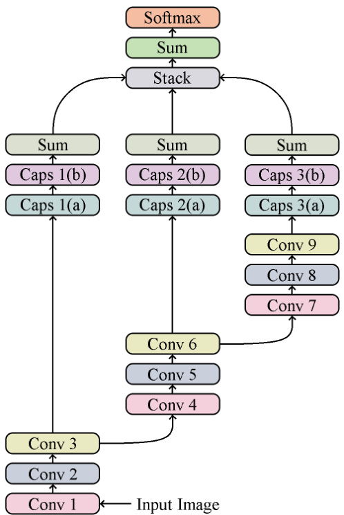
Figure 1: The proposed network from input to classification.
图 1: 从输入到分类的所提网络。
In [6], we experimented with a variety of methods for constructing the first layer of capsules out of the preceding filter maps. In this work, we limited our experiments to 2 of these methods (see Figure 2). The first method constructs each capsule from each distinct feature map (a method that, for brevity, we will refer to as XY-Derived Capsules in this work), whereas the second method constructs each capsule from each distinct $x$ and $y$ coordinate of the combination of all of the feature maps (a method that, for brevity, we will refer to as Z-Derived Capsules in this work).
在[6]中,我们尝试了多种从前置特征图构建胶囊网络首层的方法。本研究中,我们将实验范围限定为其中两种方法(见图2)。第一种方法从各独立特征图生成每个胶囊(为简洁起见,本文称之为XY派生胶囊),而第二种方法则从所有特征图组合的每个独立$x$和$y$坐标生成每个胶囊(为简洁起见,本文称之为Z派生胶囊)。
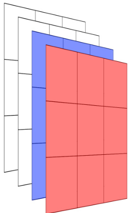
(a) In this example, the 4 filter maps have been converted into four 9-dimensional capsules, each made from an entire feature map. The first 2 of 4 such capsules are highlighted in red and blue respectively. For the sake of brevity, we will refer to this throughout the remainder of this work as using XY-Derived Capsules.
(a) 在本例中,4个滤波器映射图被转换为四个9维胶囊 (capsule),每个胶囊由整个特征图构成。其中前两个胶囊分别用红色和蓝色高亮显示。为简洁起见,在后续内容中我们将这种处理方式统称为XY派生胶囊 (XY-Derived Capsules)。
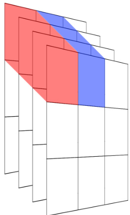
(b) In this example, the 4 filter maps have been converted into a single 4- dimensional capsule for each distinct $x$ and $y$ coordinate of the feature maps. The first 2 of 9 such capsules are highlighted in red and blue respectively. For the sake of brevity, we will refer to this throughout the remainder of this work as using Z-Derived Capsules.
(b) 在本示例中,4个滤波器映射已转换为针对特征图每个独立$x$和$y$坐标的4维胶囊。图中9个此类胶囊的前2个分别用红色和蓝色高亮显示。为简洁起见,本文后续部分将统一称之为Z派生胶囊 (Z-Derived Capsules)。
Figure 2: Illustrating the construction of capsules from $43\times3$ filter maps. These are the processes denoted by “Caps 1(a)”, “Caps 2(a)”, and “Caps 3(a)” in Figure 1.
图 2: 展示从 $43\times3$ 滤波器映射构建胶囊的过程。这些对应于图 1 中标注为 "Caps 1(a)"、"Caps 2(a)" 和 "Caps 3(a)" 的处理步骤。
We used no weight decay regular iz ation [21], a staple regular iz ation method that improves generalization by penalizing the emergence of large weight values. Nor did we use any form of dropout regular iz ation [22][23] which are regular iz ation methods designed to stop the co-adaptation of weights. We also did not use a reconstruction sub-network as in [1]. These decisions were made in order to investigate the generalization properties of our novel network design elements in the absence of other techniques associated with good generalization. In addition, we intentionally left out any form of “routing” algorithm as in [1] and [3], preferring to rely on traditional trainable weights and back propagation.
我们没有使用权重衰减正则化 [21] (一种通过惩罚大权重值出现来提升泛化能力的经典正则化方法),也未采用任何形式的dropout正则化 [22][23] (这类正则化方法旨在阻止权重间的协同适应)。同时,我们未像文献[1]那样引入重构子网络。这些设计决策是为了在剥离其他已知提升泛化性能的技术条件下,纯粹验证我们提出的新型网络架构元素的泛化特性。此外,我们刻意避开了文献[1][3]中的各类"路由"算法,选择仅依赖传统的可训练权重与反向传播机制。
3 Experimental Setup
3 实验设置
3.1 Merge Strategies
3.1 合并策略
In [8] and [9], the authors chose to give static, predetermined weights to both output branches and then added them together. In our case, for both capsules configurations from Figure 2, we conducted three separate experiments of 32 trials each in order to investigate the effects of predetermined equal weighting of the branch outputs compared to learning the branch weights via back propagation:
在[8]和[9]中,作者选择为两个输出分支赋予静态预定义权重后进行相加。针对图2中的两种胶囊配置,我们分别进行了三组实验(每组32次试验),以研究分支输出预定义等权重方案与通过反向传播学习分支权重方案的效果差异:
3.2 Data Augmentation
3.2 数据增强
Most (but not all [24][25]) of the state of the art MNIST results achieved over the past decade have used data augmentation [26][23][13]. In addition to the network design, a major part of our work involved applying an effective data augmentation strategy that included transformations informed specifically by the domain of the data. For example, we wanted to be sure we did not rotate our images into being more like a different class (e.g. rotating an image of the digit 2 by 180 degrees to create something that would more closely resemble a malformed 5). Nor did we want to translate the image content off of the canvas and perhaps cut off the left side of an 8 and thus create a 3. Choosing data augmentation techniques specific to the domain of interest is not without precedent (see for example [13] and [1], both of which used data augmentation techniques specific to MNIST).
过去十年间,大多数(但非全部[24][25])最先进的MNIST研究成果都采用了数据增强技术[26][23][13]。除网络设计外,我们工作的主要部分在于实施了一套针对数据领域特性定制的高效数据增强策略。例如,我们需要确保图像旋转不会导致类别混淆(如将数字2旋转180度生成类似畸形5的图像),同时避免平移操作使图像内容移出画布(如截断数字8左侧形成类似3的图案)。这种针对特定领域选择数据增强方法并非没有先例(参见[13]和[1],两者均采用了专为MNIST设计的数据增强技术)。
By modern standards, in terms of dataset size, MNIST has a relatively low number of training images. As such, judicious use of appropriate data augmentation techniques is important for achieving a high level of general iz ability in a given model. In terms of structure, hand-written digits show a wide variety in their rotation relative to some shared true “north”, position within the canvas, width relative to their height, and the connected ness of the strokes used to create them. Throughout training for all trials, every training image in every epoch was subjected to a series of four operations in order to simulate a greater variety of the values for these properties.
以现代标准衡量,MNIST 的训练图像数量相对较少。因此,明智地采用适当的数据增强技术对于模型实现高水平泛化能力至关重要。从结构上看,手写数字在以下方面表现出高度多样性:相对于共同基准方向的旋转角度、画布中的位置、宽高比以及笔画连贯性。在所有试验的训练过程中,每个 epoch 的每张训练图像都会经过四种操作处理,以模拟这些属性的更广泛取值。
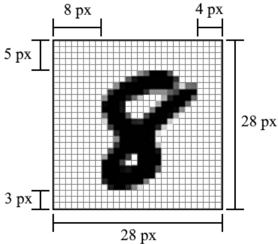
Figure 3: Example MNIST digit w/annotated margins.
图 3: 带标注边距的MNIST数字示例。
- Width. Third, we randomly adjusted each training image’s width. MNIST images are normalized to be within a $20\times20$ central patch of the $28\times28$ canvas. This normalization is ratio-preserving, so all images are 20 pixels in the height dimension but vary in the number of pixels in the width dimension. This variance not only occurs across digits, but intra-class as well, as different peoples’ handwriting can be thinner or wider than average. In order to train on a wider variety of these widths, we randomly compressed each image’s width and then added equal zero padding on either side, leaving the digit’s center where it was prior. This was inspired by a similar approach adopted in [13]. In our work, we compressed the width of each sample randomly within a range of $0-25%$ .
- 宽度。第三,我们随机调整了每张训练图像的宽度。MNIST图像被归一化到$28\times28$画布的$20\times20$中心区域内。这种归一化保持了比例不变,因此所有图像在高度维度上均为20像素,但在宽度维度上的像素数各不相同。这种差异不仅存在于不同数字之间,同类数字内部也存在,因为不同人的笔迹可能比平均值更细或更宽。为了训练模型适应更丰富的宽度变化,我们随机压缩每张图像的宽度,然后在两侧添加等量零填充,保持数字中心位置不变。这一方法灵感来源于[13]采用的类似策略。在本研究中,我们将每个样本的宽度随机压缩$0-25%$的范围。
- Random Erasure. Fourth, we randomly erased (setting to 0) a $4\times4$ grid of pixels chosen from the central $20\times20$ grid of pixels in each training image. The $\mathrm{X}$ and $\mathrm{Y}$ coordinates of the patch were drawn independently from a random uniform distribution. This was inspired by the random erasing data augmentation method in [27]. The intention behind this method was to expose the model to a greater variety of (simulated) connected ness within the strokes that make up the digits. An alternative interpretation would be to see this as a kind of feature-space dropout.
- 随机擦除。 第四,我们在每个训练图像中心 $20\times20$ 像素网格内随机选取一个 $4\times4$ 像素网格进行擦除(置零)。 该补丁的 $\mathrm{X}$ 和 $\mathrm{Y}$ 坐标从随机均匀分布中独立抽取。 该方法灵感来源于[27]提出的随机擦除数据增强技术。 其设计初衷是让模型接触更多笔画连接方式的(模拟)变体,这些笔画构成了数字。 另一种理解方式可将其视为特征空间层面的dropout。
3.3 Training
3.3 训练
We followed the training methodology from [6] and trained with the Adam optimizer [28] using all of the default/recommended parameter values, including the base learning rate of 0.001. Also, as in both [6] and [1], we exponentially decayed the base learning rate. For our experiments, which trained for 300 epochs, we applied an exponential decay to the learning rate at a rate of 0.98 per epoch.
我们遵循[6]中的训练方法,使用Adam优化器[28]进行训练,采用全部默认/推荐参数值(包括0.001的基础学习率)。与[6]和[1]相同,我们对基础学习率进行了指数衰减。在300轮训练的实验中,我们以每轮0.98的速率对学习率实施指数衰减。
Test accuracy was measured using the exponential moving average of prior weights with a decay rate of 0.999. [29]
测试准确率采用权重指数移动平均法测量,衰减率为0.999。[29]
4 Experimental Results
4 实验结果
4.1 Individual Models
4.1 个体模型
For both of the capsule construction methods (see Figure 2) and each of the three merge strategies (see subsection 3.1) we ran 32 trials. Each trial had weights randomly initialized prior to training and, due to the stochastic nature of the data augmentation, a different set of training images. As a result, training progressed to different points in the loss surface resulting in a range of values for the top accuracies that were achieved on the test set. See Table 1.
对于两种胶囊构建方法(参见图2)和三种合并策略(参见3.1小节)的每种组合,我们进行了32次试验。每次试验在训练前都随机初始化权重,并且由于数据增强的随机性,训练图像集也不同。因此,训练过程会到达损失曲面的不同位置,导致在测试集上获得的最高准确率存在一定范围的波动。参见表1。
Table 1: Test Accuracy of the Individual Models
表 1: 各独立模型的测试准确率
| HVC配置 | 实验 | 最小值 | 最大值 | 均值 | 标准差 |
|---|---|---|---|---|---|
| 使用XY衍生胶囊 | NotLearnable | 99.71% | 99.79% | 0.997500 | 0.0002190 |
| RandomInit. | 99.72% | 99.78% | 0.997512 | 0.0001499 | |
| Ones Init. | 99.70% | 99.77% | 0.997397 | 0.0001885 | |
| 使用Z衍生胶囊 | NotLearnable | 99.74% | 99.81% | 0.997731 | 0.0001825 |
| RandomInit. | 99.73% | 99.80% | 0.997684 | 0.0002023 | |
| Ones Init. | 99.72% | 99.83% | 0.997747 | 0.0002509 |
In all cases, using the Z-Derived Capsules was superior to using the XY-Derived Capsules. For Z-Derived Capsules, no merge strategy produced statistically significantly superior test accuracy. For XY-Derived Capsules, the only statistically significant test accuracy result was that the Ones Init. strategy produced inferior accuracy. It should be noted that, though no strategy produced statistically significantly superior test accuracies, when branches were allowed to learn their weights, the weights learned were statistically significant. (Bold indicates a surpassing of the previous state of the art for individual models on MNIST.) (SD abbreviates Standard Deviation)
在所有情况下,使用Z派生胶囊 (Z-Derived Capsules) 的表现均优于XY派生胶囊 (XY-Derived Capsules)。对于Z派生胶囊,没有任何合并策略能在测试准确率上产生统计学显著优势。对于XY派生胶囊,唯一具有统计学显著性的测试准确率结果是Ones Init.策略表现较差。需要指出的是,尽管没有策略能带来统计学显著更高的测试准确率,但当允许分支学习其权重时,所学得的权重具有统计学显著性。(加粗部分表示该模型在MNIST数据集上超越了先前单个模型的最优水平。) (SD为标准差缩写)
4.2 Ensembles
4.2 集成方法
Ensembling multiple models together and predicting based on the majority vote among the ensembled models routinely outperforms the individual models’ performances. Ensembling can refer to either completely different model architectures with different weights or the same model architecture after being trained multiple times and finding different sets of weights that correspond to different locations in the loss surface. The previous state of the art of $99.82%$ was achieved using an ensemble of 30 different randomly generated model architectures [30]. Our ensembling method used the same architecture but with different weights. We calculated the majority vote of the predictions for all possible combinations of the weights produced by the 32 trials. See Table 2.
将多个模型集成在一起,并通过集成模型中的多数投票进行预测,其性能通常优于单个模型的表现。集成可以指完全不同的模型架构(具有不同权重),也可以指同一模型架构经过多次训练后找到对应于损失曲面不同位置的多组权重。此前99.82%的最先进结果是通过集成30种不同随机生成的模型架构实现的[30]。我们的集成方法使用相同架构但不同权重,计算了32次试验产生的所有权重组合的预测多数投票结果。见表2。
Table 2: Test Accuracy of the Ensembles
Shown here are the number of ensembles that were generated that either matched the previous state of the art of $99.82%$ or exceeded it.
表 2: 集成模型的测试准确率
| 99.87% | 99.86% | 99.85% | 99.84% | 99.83% | 99.82% | |
|---|---|---|---|---|---|---|
| 使用XY衍生的胶囊 | ||||||
| NotLearnable | 0 | 0 | 0 | 0 | 4 | 1,183 |
| RandomInit. | 0 | 0 | 0 | 0 | 21 | 2,069 |
| OnesInit. | 0 | 0 | 0 | 1 | 19 | 1,292 |
| 使用Z衍生的胶囊 | ||||||
| NotLearnable | 184 | 4,029 | 89,384 | 1,587,152 | 17,746,467 | 121,731,146 |
| Random Init. | 0 | 1,226 | 533,318 | 17,319,668 | 148,600,238 | 554,104,195 |
| OnesInit. | 64 | 9,920 | 1,113,217 | 34,635,994 | 426,947,909 | 1,279,126,811 |
这里展示的是达到或超过先前最高水平 $99.82%$ 的集成模型数量。
4.3 Branch Weights
4.3 分支权重
What follows are visualization s of the final branch weights (after 300 epochs of training) for each of the branches in all 32 trials of the experiment wherein the branch weights were initialized to one for both HVC configurations.
以下是实验中所有32次试验的最终分支权重(经过300个训练周期后)的可视化结果,其中两种HVC配置的分支权重初始值均设为1。
In Figure 4, we see that for all trials, the ratio between the all three learned branch weights is consistent, demonstrating that the amount of contribution from each branch plays a significant role. In Figure 5, we see a similar, though less pronounced consistency between the first branch’s weight and the other two branches, however, branches two and three show no significant difference. Strikingly, when using XY-Derived Capsules we see that branch three (the one having gone through all nine convolutions) has learned to be a more significant contributor. When using Z-Derived Capsules, branch one (the one having gone through only three convolutions) has learned to be a more significant contributor, but only slightly. Indeed, in the latter configuration, the contributions from all three branches is much more equal.
在图4中,我们看到所有试验中三个学习分支权重的比例保持一致,表明每个分支的贡献量起着重要作用。图5显示第一分支权重与其他两个分支之间存在相似但较不明显的关联性,然而第二和第三分支之间没有显著差异。引人注目的是,使用XY派生胶囊时,第三分支(经过全部九次卷积的路径)贡献度显著提升;而使用Z派生胶囊时,第一分支(仅经过三次卷积的路径)贡献度仅略微增加。实际上,后一种配置中三个分支的贡献度更为均衡。
The experiments with randomly initialized branch weights showed the same relative weight of the branches for the magnitude of the weights learned. However, when the initial random branch weight was a negative number, it learned the negative value of that magnitude, and back propagation took care of flipping the signs of weights as needed further up the network.
随机初始化分支权重的实验显示,各分支在学习权重大小上具有相同的相对权重。然而,当初始随机分支权重为负数时,网络会学习该大小的负值,反向传播会根据需要在网络更高层调整权重的符号。

Figure 4: Final branch weights (after 300 epochs) for all 32 trials of the experiment using XYDerived Capsules and for which the branch weights were initialized to one.
图 4: 使用 XYDerived Capsules 进行的所有 32 次实验中最终分支权重 (经过 300 个训练周期) 的结果,这些实验的分支权重初始值均设为 1。

Figure 5: Final branch weights (after 300 epochs) for all 32 trials of the experiment using Z-Derived Capsules and for which the branch weights were initialized to one.
图 5: 使用Z-Derived Capsules进行的所有32次实验中最终分支权重(经过300个训练周期)的分布情况,这些实验的分支权重初始值均设为1。
Because the models using Z-Derived Capsules are clearly superior to XY-Derived Capsules, unless otherwise stated, all analyses throughout the remainder of this work will restrict attention to these 96 trials, and thus, when the text reads “all 96 trials”, it should be understood that this refers to all 96 trials using Z-Derived Capsules.
由于采用Z轴衍生胶囊(Z-Derived Capsules)的模型明显优于XY轴衍生胶囊,除非另有说明,本文后续所有分析将仅关注这96次试验。因此,文中提及"全部96次试验"时,均特指使用Z轴衍生胶囊的96次试验。
4.4 Troublesome Digits
4.4 棘手的数字
Across all 96 trials there was total agreement on 9,912 out of the 10,000 test samples. There were only 14 digits that were mis classified more often than not across all 96 trials. This shows that although the accuracies of the models in the three experiments were quite similar, the different merge strategies of the three experiments did have a significant effect on classification. Across all 96 trials, only 5 samples were mis classified in all models. Those samples, as numbered by the order they appear in the MNIST test dataset (starting from 0) are 1901, 2130, 2597, 3422, and 6576.
在全部96次试验中,10,000个测试样本中有9,912个达成完全一致分类。仅有14个数字在超过半数试验中被误判。这表明尽管三个实验中的模型准确率非常接近,但不同的合并策略对分类结果产生了显著影响。所有试验中仅有5个样本被全部模型误判,这些样本按MNIST测试集出现顺序编号(从0开始)分别为1901、2130、2597、3422和6576。

Figure 6: The Most Troublesome Digits
图 6: 最难识别的数字
4.5 MNIST State of the Art
4.5 MNIST 最新技术进展
In Table 3 we present a comparison of previous state of the art MNIST results for both single model evaluations and ensembles along with the results achieved in our experiments.
表3: 我们展示了先前最先进的MNIST单模型评估与集成方法结果,并与本实验所得结果进行对比。
Table 3: Current and Previous MNIST State of the Art Results
表 3: 当前与先前 MNIST 最佳结果对比
| 论文 | 年份 | 准确率 |
|---|---|---|
| 单模型 | ||
| Dynamic Routing Between Capsules [1] | 2017 | 99.75% |
| Let's keep it simple, Using simple architectures to outperform deeper and more complex architectures [24] | 2016 | 99.75% |
| Batch-Normalized Maxout Network in Network [25] | 2015 | 99.76% |
| APAC: Augmented PAttern Classification with Neural Networks [26] | 2015 | 99.77% |
| Multi-Column Deep Neural Networks for Image Classification [13] | 2012 | 99.77% |
| 采用本工作提出的方法 | 2021 | 99.83% |
| 集成模型 | ||
| Regularization of Neural Networks using DropConnect [23] | 2013 | 99.79% |
| RMDL: Random Multimodel Deep Learning for Classification [30] | 2018 | 99.82% |
| 采用本工作提出的集成方法 | 2021 | 99.87% |
How long a model takes to train is an important factor to consider when evaluating a neural network. Indeed, it is an enabling factor during initial experimentation as faster training leads to a greater exploration of the design space. In Table 4 we present a comparison of the number of epochs of training used in experiments for the results achieved in the networks shown in Table 3. Across all 96 trials, the design achieved peak accuracy in an average of 168 epochs, with a minimum peak achieved in 38 epochs and a maximum peak achieved at epoch 296. Since, all trials were allowed to run for up to 300 epochs, that is the number reported in Table 4.
在评估神经网络时,模型的训练时长是一个重要考量因素。实际上,它在初期实验中起到关键推动作用,因为更快的训练速度能带来更广阔的设计空间探索。表4展示了为实现表3中网络结果所采用的训练周期数对比。在全部96次试验中,该设计平均经过168个周期达到峰值准确率,最短38个周期即达峰值,最长则需要296个周期。由于所有试验均被允许运行至多300个周期,因此表4中统一报告该数值。
4.6 Interpreting Capsules’ Dimensions
4.6 解读胶囊的维度
By adding a reconstruction sub-network to the overall network, it can be trained not just to classify the input digits, but also to reconstruct them. Then, by following the method in [1], we can examine the effects of perturbing individual dimensions of the second set of capsules in a pair of HVCs. The experiments using Z-Derived Capsules had capsules with 64, 112, and 160 dimensions. When perturbing only one of that many dimensions the changes to the resulting constructed images are very subtle. So we ran another experiment with no branches, reconstruction, and using multiple 8-dimensional capsules for each distinct $x$ and $y$ coordinate of the feature maps. By perturbing one of only eight dimensions the effects are more visible and allows us to interpret the meaning of values in the digits’ capsules (see Table 5).
通过在整体网络中添加一个重建子网络,可以训练其不仅能对输入数字进行分类,还能重建它们。接着,按照[1]中的方法,我们可以研究扰动一对HVC中第二组胶囊的单个维度所产生的影响。使用Z-Derived Capsules的实验采用了64、112和160维的胶囊。当仅扰动众多维度中的一个时,重构图像的改变非常细微。因此,我们进行了另一项实验,不使用分支和重建,而是为特征图的每个不同$x$和$y$坐标使用多个8维胶囊。通过仅扰动八个维度中的一个,效果更加明显,使我们能够解释数字胶囊中值的含义(见表5)。
Table 4: Epochs of Training
Neither [24] nor [25] report on how many epochs their designs were trained for.
表 4: 训练轮次
| 论文 | 训练轮次 |
|---|---|
| DynamicRoutingBetween Capsules[1] | 1,200 |
| APAC:Augmented PAttern ClassificationwithNeuralNetworks[26] | 15.000 |
| Multi-Column Deep Neural Networks for Image Classification[13] | 800 |
| Regularization of Neural Networks using DropConnect[23] | 1,200 |
| RMDL:Random Multimodel Deep Learning for Classification[30] | 120 |
| The method proposed in this work | 300 |
[24]和[25]均未报告其设计的训练轮次。
Table 5: Dimensional Perturbations
Each row shows the reconstruction when one of the 8 dimensions in a digit’s capsule is perturbed by intervals of 0.1 in the range [-0.5, 0.5].
表 5: 维度扰动
| 向右倾斜 | |
| 顶部卷曲及下部环高度 | 8882222222 |
| 下部笔画长度 | 3333333333 |
| 单笔画顶部角度 | hhhhhh |
| 下部双曲线角度锐度 | |
| 整体数字宽度 | 99999 |
| 笔画起始部分的"钩" | 777777 |
| 下部环宽度 | 88888888 |
| 倾斜角度 | 9999999 A |
每行展示当数字胶囊中8个维度之一在[-0.5, 0.5]范围内以0.1为间隔扰动时的重建结果。
4.7 Ablation Experiments
4.7 消融实验
In each of the following set of experiments, we compared the first 10 trials of the 32 trials for the Ones Init. merge strategy with 10 trials each of the additional experiments.
在以下每组实验中,我们将Ones Init合并策略的32次试验中的前10次,与其他各项实验的10次试验进行对比。
In [1], the authors used a custom loss function they called margin loss combined with the mean squared error of the difference between the input images and the result of reconstructing them. In our work and with our design, we chose to rely solely on categorical cross-entropy and not to use a reconstruction loss, as reconstruction adds a considerable number of parameters to the model (2.1M). We ran two additional experiments to understand the effect of our choice of loss strategy (which used categorical cross-entropy and no reconstruction). The first used margin loss and reconstruction, and the second used categorical cross-entropy and reconstruction. There was no statistically significant difference among the three loss methods (see Table 6).
在[1]中,作者采用了一种自定义的边际损失函数(margin loss),并结合输入图像与重建结果之间的均方误差。而在我们的研究和设计中,我们选择仅依赖分类交叉熵,不使用重建损失,因为重建会给模型增加大量参数(210万)。我们进行了两组补充实验来验证损失策略选择(仅使用分类交叉熵且无重建)的影响:第一组采用边际损失加重建,第二组采用分类交叉熵加重建。三种损失方法之间不存在统计学显著差异(见表6)。
Table 6: Comparison of Loss Methods
表 6: 损失方法对比
| 损失方法 | 平均准确率 | 标准差 |
|---|---|---|
| 分类交叉熵 (无重建) | 99.7741% | 0.000186455 |
| 分类交叉熵 (带重建) | 99.7740% | 0.000245764 |
| 间隔损失 (带重建) | 99.7820% | 0.000198997 |
In order to understand the relative importance of using HVCs vs. a fully connected layer and 3 branches vs. a single branch, we ran a series of experiments that ablated these components of the architecture. Table 7 shows that HVCs are statistically significantly superior to a fully connected layer for both 1 and 3 branches, and shows that 3 branches are superior to 1 branch for both HVCs and a fully connected layer.
为了理解使用HVC (Hierarchical View Convolution) 与全连接层、3分支结构与单分支结构的相对重要性,我们进行了一系列消融实验来验证这些架构组件的影响。表7显示,无论是1分支还是3分支结构,HVC在统计显著性上都优于全连接层;同时,无论采用HVC还是全连接层,3分支结构均优于单分支结构。
Table 7: Comparison of Network Structures
表 7: 网络结构对比
| 网络结构 | 平均准确率 | 标准差 |
|---|---|---|
| 使用HVCs和3分支 | 99.7741% | 0.000186455 |
| 使用HVCs和1分支 | 99.7140% | 0.000185472 |
| 使用全连接层和3分支 | 99.7550% | 0.000111803 |
| 使用全连接层和1分支 | 99.6870% | 0.000141774 |
In [1], the authors used translation, by a maximum of 2-pixels, as the only data augmentation method. In our work, we devised a method for translating by up to the full margin available in any given direction. We compared the effect of using only 2-pixel translation, only maximum margin translation, and our full suite of data augmentation methods. Using the full suite of data augmentation methods was shown to be statistically superior to either of the other two methods. Much to our surprise, we found that the 2-pixel translation method just barely crossed the threshold of being statistically significantly superior to the full margin translation method (see Table 8).
在[1]中,作者仅采用最大2像素平移作为唯一的数据增强方法。本研究中,我们开发了一种可在任意方向实现全边距平移的方法。通过对比仅使用2像素平移、仅使用最大边距平移以及完整数据增强方案的效果,结果表明采用完整数据增强方案在统计上显著优于前两种方法。令人意外的是,2像素平移法仅以微弱优势跨过统计显著性阈值,略优于全边距平移法 (见表8)。
The result we obtained by when using 2-pixel translation as the only data augmentation strategy allows for a direct comparison to the work of [1]. We obtained the same level of accuracy as they did, but using $5.5\times$ fewer parameters, $4\times$ fewer training epochs, no reconstruction sub-network, and requiring no routing mechanism.
我们仅使用2像素平移作为数据增强策略得到的结果,可直接与[1]的研究进行对比。在达到相同准确率的同时,我们的方法参数减少了5.5倍、训练周期缩短了4倍,且无需重建子网络和路由机制。
Table 8: Comparison of Data Augmentation Strategies
表 8: 数据增强策略对比
| 数据增强策略 | 平均准确率 | 标准差 |
|---|---|---|
| 平移(全边界)、旋转、宽度调整和随机擦除 | 99.7741% | 0.000186455 |
| 仅平移(最大2像素) (如[1]所述) | 99.7570% | 0.000195192 |
| 仅平移(使用全边界) | 99.7430% | 0.000118743 |
4.8 Additional Datasets
4.8 其他数据集
In order to better understand the effect of the Z-Derived HVCs and additional branches, we ran additional sets of paired experiments for several additional datasets wherein the first set of experiments in a pair used the network design as described in this work and the second set of experiments excluded the Z-Derived HVCs and additional branches. These second sets of experiments thus use a very small and typical convolutional neural network with $93\times3$ convolutions and a final fully connected layer.
为了更好地理解Z-Derived HVCs和附加分支的效果,我们针对多个额外数据集运行了多组成对实验:每组实验中的第一组采用本文所述的网络设计,第二组则移除Z-Derived HVCs和附加分支。因此第二组实验仅使用极简的典型卷积神经网络架构,包含 $93\times3$ 卷积层和最终全连接层。
For MNIST and Fashion-MNIST we used the data augmentation strategy discussed in subsection 3.2. For CIFAR-10 and CIFAR-100, this data augmentation strategy is inappropriate, so we used a very typical strategy of randomly flipping the images horizontally and applying random adjustments to brightness, contrast, hue, and saturation.
对于MNIST和Fashion-MNIST数据集,我们采用了3.2小节讨论的数据增强策略。而对于CIFAR-10和CIFAR-100数据集,该策略并不适用,因此我们采用了更典型的增强方法:随机水平翻转图像,并对亮度、对比度、色调和饱和度进行随机调整。
For all four datasets, the model that included Z-Derived HVCs and 3 branches achieved the higher mean accuracy with statistical significance (see Table 9).
在全部四个数据集中,包含Z-Derived HVCs和三分支结构的模型均以统计显著性获得了更高的平均准确率 (见表9)。
The fact that the accuracies for Fashion-MNIST [31], CIFAR-10, and CIFAR-100 [32] were not competitive with current state of the art for those datasets is not especially surprising for several reasons. First, our network was designed for optimal accuracy on classification of Arabic numerals which are highly structured and significantly simpler than the types of data in the other three datasets. Second, due to the significantly simpler nature of MNIST, we used a small number of parameters for our network (1.5M). For comparison, models competitive with state of the art for CIFAR-10 and CIFAR-100 use 10s and even 100s of millions of parameters. Finally, models competitive with state of the art for CIFAR-10 and CIFAR-100 use additional training data beyond the canonical set for each, and we used no additional training data.
Fashion-MNIST [31]、CIFAR-10和CIFAR-100 [32]的准确率未达到这些数据集当前最先进水平,这一事实并不特别令人意外,原因如下。首先,我们的网络专为阿拉伯数字分类而设计,这些数字具有高度结构化且比其他三个数据集中的数据类型简单得多。其次,由于MNIST的复杂性显著较低,我们为网络使用了少量参数(150万)。作为对比,在CIFAR-10和CIFAR-100上达到最先进水平的模型使用了数千万甚至数亿参数。最后,这些先进模型还使用了各自标准训练集之外的额外数据,而我们未使用任何额外训练数据。
Table 9: Effects of Z-Derived HVCs and Branching on Additional Datasets
MNIST results come from the same experiments detailed in Table 7 and are repeated here to facilitate ease of comparison We conducted 10 trials of each unique type of experiment in order to establish statistical significance.
表 9: Z派生HVC和分支结构在附加数据集上的效果
| 数据集 | 网络架构 | 最大值 | 平均值 | 标准差 | p值 |
|---|---|---|---|---|---|
| MNIST | Z派生HVC和3分支 | 99.81% | 99.7741% | 0.0001864 | 1.824 × 10⁻⁷ |
| 全连接层和1分支 | 99.71% | 99.6870% | 0.0001417 | ||
| Fashion-MNIST | Z派生HVC和3分支 | 93.89% | 93.6850% | 0.0016391 | 5.243 × 10⁻⁶ |
| 全连接层和1分支 | 93.36% | 93.0410% | 0.0014616 | ||
| CIFAR-10 | Z派生HVC和3分支 | 89.23% | 88.9290% | 0.0015514 | 0.020898 |
| 全连接层和1分支 | 89.06% | 88.7500% | 0.0017515 | ||
| CIFAR-100 | Z派生HVC和3分支 | 64.15% | 63.8260% | 0.0026743 | 6.859 × 10⁻⁶ |
| 全连接层和1分支 | 62.96% | 62.3760% | 0.0035046 |
MNIST结果来自表7所述相同实验,为便于比较在此重复列出。我们为每种实验类型进行了10次试验以确立统计显著性。
5 Conclusion
5 结论
In this work, we proposed using a simple convolutional neural network and established design principles as a basis for a network architecture. We then presented a design that branched out of the series of stacked convolutions at different points to capture different levels of abstraction and effective receptive fields, and from these branches, rather than flattening to individual scalar neurons, used Homogeneous Vector Capsules instead.
在本工作中,我们提出使用简单的卷积神经网络并建立设计原则作为网络架构的基础。随后展示了一种设计:在不同节点从堆叠卷积序列中分支出多条路径,以捕捉不同层次的抽象特征和有效感受野。这些分支并非展平为单个标量神经元,而是采用同质向量胶囊 (Homogeneous Vector Capsules) 结构。
We also investigated three different methods of merging the output of the branches back into a single set of logits. Each of the three merge strategies generated models that could be ensembled to create new state of the art results.
我们还研究了三种不同的方法将分支输出合并回单一logits集合。这三种合并策略生成的模型均可通过集成方法创造出新的最先进成果。
Beyond the network architecture, we proposed a robust and domain specific data augmentation strategy aimed at simulating a wider variety of renderings of the digits.
除了网络架构之外,我们提出了一种鲁棒且针对特定领域的数据增强策略,旨在模拟数字更广泛的渲染效果。
In doing this work, we established new MNIST state of the art accuracies for both a single model and an ensemble. In addition to the network design and augmentation strategy, the ability to use an adaptive gradient descent method [6] allowed us to achieve this on consumer hardware (2x NVIDIA GeForce GTX 1080 Tis in an otherwise unremarkable workstation) and was an enabling factor in both initial explorations and the training of all 322 trials of experiments referenced in this work.
在进行这项工作时,我们为单一模型和集成模型均建立了新的MNIST最高准确率记录。除了网络设计和数据增强策略外,使用自适应梯度下降方法 [6] 的能力使我们能够在消费级硬件(工作站中配置的2块NVIDIA GeForce GTX 1080 Ti显卡)上实现这一目标,这也是本工作引用的322次实验初始探索和全部训练过程中的关键赋能因素。
References
参考文献
[32] A. Krizhevsky. Learning Multiple Layers of Features from Tiny Images. Tech. rep. 2009.
[32] A. Krizhevsky. 从微小图像中学习多层特征. 技术报告. 2009.
The code used for all experiments and summary level data is publicly available on GitHub at: https://github.com/AdamByerly/BMCNNwHFCs
所有实验和汇总级数据所使用的代码已在GitHub上公开:https://github.com/AdamByerly/BMCNNwHFCs
A Appendix
附录
A.1 Digits Disagreed Upon
A.1 存在分歧的数字
What follows is the complete set of 88 digits that were predicted correctly by at least one model and incorrectly by at least one model. These in combination with the digits from Figure 6 represent the complete set of digits that were not predicted correctly by all 96 trials. Each image is captioned first by the class label in the test data set associated with the image, then the number of trials that predicted it correctly, and last the index of the digit in the test data. For example, the first image presented below has a class label of 3, 95 trials predicted that correctly, and it exists at index 87 in the MNIST test data.
以下是至少一个模型预测正确且至少一个模型预测错误的88个数字的完整集合。这些数字与图6中的数字共同构成了所有96次试验中未能全部预测正确的数字全集。每张图片的说明依次为:测试数据集中与该图片关联的类别标签、预测正确的试验次数,以及该数字在测试数据中的索引。例如,下面展示的第一张图片类别标签为3,有95次试验预测正确,它在MNIST测试数据中的索引为87。
