Combining Deep Reinforcement Learning and Search for Imperfect-Information Games

结合深度强化学习与搜索应对非完美信息博弈

Noam Brown∗ Anton Bakhtin∗ Adam Lerer Qucheng Gong Facebook AI Research {noambrown,yolo,alerer,qucheng}@fb.com

Abstract

摘要

The combination of deep reinforcement learning and search at both training and test time is a powerful paradigm that has led to a number of successes in single-agent settings and perfect-information games, best exemplified by AlphaZero. However, prior algorithms of this form cannot cope with imperfect-information games. This paper presents ReBeL, a general framework for self-play reinforcement learning and search that provably converges to a Nash equilibrium in any two-player zerosum game. In the simpler setting of perfect-information games, ReBeL reduces to an algorithm similar to AlphaZero. Results in two different imperfect-information games show ReBeL converges to an approximate Nash equilibrium. We also show ReBeL achieves superhuman performance in heads-up no-limit Texas hold’em poker, while using far less domain knowledge than any prior poker AI.

深度强化学习与训练及测试时搜索的结合是一种强大范式，已在单智能体环境和完美信息博弈中取得多项突破性成果，AlphaZero 便是最佳例证。然而，此类现有算法无法处理非完美信息博弈。本文提出ReBeL框架——一种自博弈强化学习与搜索的通用框架，可证明能在任何两人零和博弈中收敛至纳什均衡。在完美信息博弈的简化场景下，ReBeL会退化为类似AlphaZero的算法。两个不同非完美信息博弈的实验表明，ReBeL能收敛至近似纳什均衡。我们还证明ReBeL在无限注德州扑克单挑对局中实现了超越人类的表现，且所需领域知识远少于以往任何扑克AI。

1 Introduction

1 引言

Combining reinforcement learning with search at both training and test time $\mathbf{RL+}$ Search) has led to a number of major successes in AI in recent years. For example, the AlphaZero algorithm achieves state-of-the-art performance in the perfect-information games of Go, chess, and shogi [55].

结合强化学习与训练和测试阶段的搜索（RL+搜索）近年来在人工智能领域取得了一系列重大突破。例如，AlphaZero算法在围棋、国际象棋和将棋等完美信息博弈中实现了最先进的性能[55]。

However, prior $\mathrm{RL}+\mathrm{S}$ earch algorithms do not work in imperfect-information games because they make a number of assumptions that no longer hold in these settings. An example of this is illustrated in Figure 1a, which shows a modified form of Rock-Paper-Scissors in which the winner receives two points (and the loser loses two points) when either player chooses Scissors [15]. The figure shows the game in a sequential form in which player 2 acts after player 1 but does not observe player 1’s action.

然而，现有的 $\mathrm{RL}+\mathrm{S}$ 搜索算法在非完美信息博弈中失效，因为它们依赖的若干假设在此类场景下不再成立。图 1a 展示了一个改编版的石头剪刀布游戏：当任意一方选择剪刀时，胜者得两分（败者扣两分）[15]。该图以序贯形式呈现游戏流程——玩家2在玩家1行动后做出决策，但无法观测到玩家1的选择。

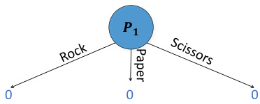
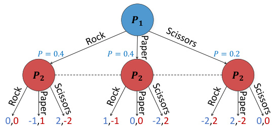
(1a) Variant of Rock-Paper-Scissors in which the opti- (1b) The player 1 subgame when using perfectmal player 1 policy is $(\mathrm{R}{=}0.4$ , $\mathrm{P{=}0.4}$ , $\mathrm{S}{=}0.2$ ). Terminal information one-ply search. Leaf values are detervalues are color-coded. The dotted lines mean player 2 mined by the full-game equilibrium. There is insuffidoes not know which node they are in. cient information for finding $\mathrm{R=0.4}$ , $\mathrm{P{=}0.4}$ , $\scriptstyle{\mathrm{S}=0.2}$ ).

图 1:
(1a) 石头剪刀布的变体游戏，其中最优玩家1策略为 $(\mathrm{R}{=}0.4$ , $\mathrm{P{=}0.4}$ , $\mathrm{S}{=}0.2$ )。终端信息值用颜色编码。虚线表示玩家2不知道所处节点。
(1b) 使用完美单层搜索时的玩家1子博弈。叶节点值由完整游戏均衡确定。缺乏足够信息来找到 $\mathrm{R=0.4}$ , $\mathrm{P{=}0.4}$ , $\scriptstyle{\mathrm{S}=0.2}$ )。

The optimal policy for both players in this modified version of the game is to choose Rock and Paper with $40%$ probability, and Scissors with $20%$ . In that case, each action results in an expected value of zero. However, as shown in Figure 1b, if player 1 were to conduct one-ply lookahead search as is done in perfect-information games (in which the equilibrium value of a state is substituted at a leaf node), then there would not be enough information for player 1 to arrive at this optimal policy.

在这个修改版的游戏中，双方玩家的最优策略是以40%的概率选择石头和布，以20%的概率选择剪刀。在这种情况下，每个动作的期望值为零。然而，如图1b所示，如果玩家1像完全信息博弈那样进行一步前瞻搜索（即在叶节点处用状态的均衡值替代），那么玩家1将无法获得足够信息来得出这一最优策略。

This illustrates a critical challenge of imperfect-information games: unlike perfect-information games and single-agent settings, the value of an action may depend on the probability it is chosen. Thus, a state defined only by the sequence of actions and observations does not have a unique value and therefore existing RL+Search algorithms such as AlphaZero are not sound in imperfectinformation games. Recent AI breakthroughs in imperfect-information games have highlighted the importance of search at test time [40, 12, 14, 37], but combining RL and search during training in imperfect-information games has been an open problem.

这揭示了不完美信息博弈的一个关键挑战：与完美信息博弈和单智能体设置不同，某个行动的价值可能取决于其被选择的概率。因此，仅由行动和观察序列定义的状态并不具备唯一价值，这使得现有RL+搜索算法（如AlphaZero）在不完美信息博弈中缺乏理论保证。近期不完美信息博弈领域的AI突破凸显了测试阶段搜索的重要性[40,12,14,37]，但如何在训练过程中将强化学习与搜索相结合仍是一个悬而未决的难题。

This paper introduces ReBeL (Recursive Belief-based Learning), a general RL $^{+}$ Search framework that converges to a Nash equilibrium in two-player zero-sum games. ReBeL builds on prior work in which the notion of “state” is expanded to include the probabilistic belief distribution of all agents about what state they may be in, based on common knowledge observations and policies for all agents. Our algorithm trains a value network and a policy network for these expanded states through self-play reinforcement learning. Additionally, the algorithm uses the value and policy network for search during self play.

本文介绍ReBeL(基于递归信念的学习)，这是一个通用的强化学习(RL$^{+}$)搜索框架，可在双人零和博弈中收敛至纳什均衡。ReBeL建立在先前研究基础上，将"状态"概念扩展为包含所有智能体基于公共知识观察和策略对可能所处状态的概率信念分布。我们的算法通过自我对弈强化学习为这些扩展状态训练价值网络和策略网络。此外，该算法在自我对弈过程中利用价值网络和策略网络进行搜索。

ReBeL provably converges to a Nash equilibrium in all two-player zero-sum games. In perfectinformation games, ReBeL simplifies to an algorithm similar to AlphaZero, with the major difference being in the type of search algorithm used. Experimental results show that ReBeL is effective in large-scale games and defeats a top human professional with statistical significance in the benchmark game of heads-up no-limit Texas hold’em poker while using far less expert domain knowledge than any previous poker AI. We also show that ReBeL approximates a Nash equilibrium in Liar’s Dice, another benchmark imperfect-information game, and open source our implementation of it.2

ReBeL在所有两人零和博弈中可证明收敛至纳什均衡。在完美信息博弈中，ReBeL简化为类似AlphaZero的算法，主要区别在于所使用的搜索算法类型。实验结果表明，ReBeL在大规模博弈中表现优异，并在德州扑克单挑无限注这一基准游戏中以统计显著性击败顶尖人类职业选手，同时使用的专家领域知识远少于以往任何扑克AI。我们还证明ReBeL能在另一基准非完美信息博弈"骗子骰"中逼近纳什均衡，并开源了相关实现。[20]

2 相关工作

At a high level, ReBeL resembles past RL $^{+}$ Search algorithms used in perfect-information games [59, 56, 1, 55, 50]. These algorithms train a value network through self play. During training, a search algorithm is used in which the values of leaf nodes are determined via the value function. Additionally, a policy network may be used to guide search. These forms of RL $+$ Search have been critical to achieving superhuman performance in benchmark perfect-information games. For example, so far no AI agent has achieved superhuman performance in Go without using search at both training and test time. However, these RL $^{+}$ Search algorithms are not theoretically sound in imperfect-information games and have not been shown to be successful in such settings.

从高层次来看，ReBeL类似于过去用于完美信息博弈的RL$^{+}$搜索算法[59, 56, 1, 55, 50]。这些算法通过自我对弈训练价值网络。在训练过程中，搜索算法会使用价值函数确定叶节点值，同时可能采用策略网络来引导搜索。这类RL$+$搜索形式对实现基准完美信息博弈的超人类表现至关重要。例如，迄今为止，没有任何AI智能体能在围棋中不借助训练和测试阶段的搜索就达到超人类水平。然而，这些RL$^{+}$搜索算法在不完美信息博弈中缺乏理论依据，也尚未被证明能在此类场景中取得成功。

A critical element of our imperfect-information RL $^{+}$ Search framework is to use an expanded notion of “state”, which we refer to as a public belief state (PBS). PBSs are defined by a common-knowledge belief distribution over states, determined by the public observations shared by all agents and the policies of all agents. PBSs can be viewed as a multi-agent generalization of belief states used in partially observable Markov decision processes (POMDPs) [31]. The concept of PBSs originated in work on decentralized multi-agent POMDPs [43, 45, 19] and has been widely used since then in imperfect-information games more broadly [40, 20, 53, 29].

我们不完全信息强化学习 $^{+}$ 搜索框架的一个关键要素是使用扩展的"状态"概念，即公共信念状态 (public belief state, PBS)。PBS由对状态的共同知识信念分布定义，该分布由所有智能体共享的公共观测和所有智能体的策略决定。PBS可视为部分可观测马尔可夫决策过程 (POMDPs) [31] 中信念状态的多智能体泛化。PBS概念源于去中心化多智能体POMDPs的研究 [43, 45, 19]，此后被广泛应用于更广泛的不完全信息博弈领域 [40, 20, 53, 29]。

ReBeL builds upon the idea of using a PBS value function during search, which was previously used in the poker AI DeepStack [40]. However, DeepStack’s value function was trained not through self-play RL, but rather by generating random PBSs, including random probability distributions, and estimating their values using search. This would be like learning a value function for Go by randomly placing stones on the board. This is not an efficient way of learning a value function because the vast majority of randomly generated situations would not be relevant in actual play. DeepStack coped with this by using handcrafted features to reduce the dimensionality of the public belief state space, by sampling PBSs from a distribution based on expert domain knowledge, and by using domain-specific abstractions to circumvent the need for a value network when close to the end of the game.

ReBeL基于在搜索过程中使用公共信念状态 (PBS) 值函数的理念，这一方法曾用于扑克AI DeepStack [40]。然而，DeepStack的值函数并非通过自我对弈强化学习训练，而是通过生成随机PBS（包括随机概率分布）并利用搜索估算其值得出。这就像通过在棋盘上随机落子来学习围棋的值函数。由于绝大多数随机生成的情境与实际对局无关，这种学习方式效率低下。DeepStack通过三种方式应对该问题：使用手工设计特征降低公共信念状态空间维度、基于专家领域知识从特定分布中采样PBS，以及在接近终局时采用领域特定抽象来规避值网络的需求。

An alternative approach for depth-limited search in imperfect-information games that does not use a value function for PBSs was used in the Pluribus poker AI to defeat elite humans in multiplayer poker [15, 14]. This approach trains a population of “blueprint” policies without using search. At test time, the approach conducts depth-limited search by allowing each agent to choose a blueprint policy from the population at leaf nodes. The value of the leaf node is the expected value of each agent playing their chosen blueprint policy against all the other agents’ choice for the rest of the game. While this approach has been successful in poker, it does not use search during training and therefore requires strong blueprint policies to be computed without search. Also, the computational cost of the search algorithm grows linearly with the number of blueprint policies.

在不完美信息游戏中，Pluribus扑克AI采用了一种无需为公共信念状态(PBS)构建价值函数的深度受限搜索替代方案，从而在多人扑克比赛中击败人类精英选手[15,14]。该方法通过训练一组"蓝图"策略种群（训练阶段不使用搜索），在测试阶段通过允许每个智能体在叶节点选择种群中的蓝图策略来实现深度受限搜索。叶节点价值等于每个智能体采用所选蓝图策略与其他智能体后续策略选择进行博弈的期望值。虽然该方法在扑克领域取得成功，但由于训练阶段未使用搜索，必须预先计算出强效的蓝图策略。此外，搜索算法的计算成本会随蓝图策略数量线性增长。

3 Notation and Background

3 符号与背景

We assume that the rules of the game and the agents’ policies (including search algorithms) are common knowledge [2].3 That is, they are known by all agents, all agents know they are known by all agents, etc. However, the outcome of stochastic algorithms (i.e., the random seeds) are not known. In Section 6 we show how to remove the assumption that we know another player’s policy.

我们假设游戏规则和智能体的策略(包括搜索算法)是共同知识 [2]。也就是说，所有智能体都知道这些信息，所有智能体都知道其他智能体也知道这些信息，以此类推。然而，随机算法(即随机种子)的结果是未知的。在第6节中，我们将展示如何移除"知道其他玩家策略"这一假设。

Our notation is based on that of factored observation games [34] which is a modification of partially observable stochastic games [26] that distinguishes between private and public observations. We consider a game with $\mathcal{N}={1,2,...,N}$ agents.

我们的符号体系基于分解观测博弈 [34]，这是对部分可观测随机博弈 [26] 的改进，区分了私有观测和公共观测。我们考虑一个有 $\mathcal{N}={1,2,...,N}$ 个智能体的博弈。

A world state $w\in\mathcal{W}$ is a state in the game. $\mathcal{A}=\mathcal{A}_ {1}\times\mathcal{A}_ {2}\times\ldots\times\mathcal{A}_ {N}$ is the space of joint actions. $\mathcal{A}_ {i}(w)$ denotes the legal actions for agent $i$ at $w$ and $a=(a_{1},a_{2},...,a_{N})\in\mathcal{A}$ denotes a joint action. After a joint action $a$ is chosen, a transition function $\tau$ determines the next world state $w^{\prime}$ drawn from the probability distribution $\mathscr{T}(w,a)\in\Delta\mathcal{W}$ . After joint action $a$ , agent $i$ receives a reward $\mathcal{R}_{i}(w,a)$ .

世界状态 $w\in\mathcal{W}$ 是游戏中的一个状态。联合动作空间定义为 $\mathcal{A}=\mathcal{A}_ {1}\times\mathcal{A}_ {2}\times\ldots\times\mathcal{A}_ {N}$。$\mathcal{A}_ {i}(w)$ 表示智能体 $i$ 在状态 $w$ 下的合法动作集合，而 $a=(a_{1},a_{2},...,a_{N})\in\mathcal{A}$ 代表一个联合动作。当联合动作 $a$ 被选定后，转移函数 $\tau$ 根据概率分布 $\mathscr{T}(w,a)\in\Delta\mathcal{W}$ 确定下一个世界状态 $w^{\prime}$。执行联合动作 $a$ 后，智能体 $i$ 将获得奖励 $\mathcal{R}_{i}(w,a)$。

Upon transition from world state $w$ to $w^{\prime}$ via joint action $a$ , agent $i$ receives a private observation from a function $\mathcal{O}_ {\mathrm{priv}(i)}(w,a,w^{\prime})$ . Additionally, all agents receive a public observation from a function $\mathcal{O}_{\mathrm{pub}}(w,a,w^{\prime})$ . Public observations may include observations of publicly taken actions by agents. For example, in many recreational games, including poker, all betting actions are public.

当从世界状态 $w$ 通过联合动作 $a$ 转移到 $w^{\prime}$ 时，智能体 $i$ 会从函数 $\mathcal{O}_ {\mathrm{priv}(i)}(w,a,w^{\prime})$ 获得一个私有观察值。此外，所有智能体还会从函数 $\mathcal{O}_{\mathrm{pub}}(w,a,w^{\prime})$ 接收到一个公共观察值。公共观察值可能包括对智能体公开执行动作的观察。例如，在许多休闲游戏中（包括扑克），所有下注动作都是公开的。

A history (also called a trajectory) is a finite sequence of legal actions and world states, denoted $h=(w^{0},a^{0},w^{1},a^{1},...,w^{t})$ . An infostate (also called an action-observation history $({\bf A O H});$ for agent $i$ is a sequence of an agent’s observations and actions $s_{i}=(O_{i}^{0},a_{i}^{0},O_{i}^{1},a_{i}^{1},...,O_{i}^{t})$ where $\begin{array}{r}{\bar{O_{i}^{k}}=\left(\mathcal{O}_ {\mathrm{priv}(i)}\bar{(}w^{k-1},a^{k-1},\bar{w^{k}}),\mathcal{O}_ {\mathrm{pub}}(w^{k-1},a^{k-1},w^{k})\right)}\end{array}$ . The unique infostate corresponding to a history $h$ for agent $i$ is denoted $s_{i}(h)$ . The set of histories that correspond to $s_{i}$ is denoted $\mathcal{H}(s_{i})$ .

历史（也称为轨迹）是一个由合法动作和世界状态构成的有限序列，记作 $h=(w^{0},a^{0},w^{1},a^{1},...,w^{t})$。信息状态（也称为动作-观察历史 $({\bf A O H})$）对智能体 $i$ 而言是其观察与动作的序列 $s_{i}=(O_{i}^{0},a_{i}^{0},O_{i}^{1},a_{i}^{1},...,O_{i}^{t})$，其中 $\begin{array}{r}{\bar{O_{i}^{k}}=\left(\mathcal{O}_ {\mathrm{priv}(i)}\bar{(}w^{k-1},a^{k-1},\bar{w^{k}}),\mathcal{O}_ {\mathrm{pub}}(w^{k-1},a^{k-1},w^{k})\right)}\end{array}$。与历史 $h$ 对应的智能体 $i$ 的唯一信息状态记作 $s_{i}(h)$，而对应于 $s_{i}$ 的所有历史集合记作 $\mathcal{H}(s_{i})$。

A public state is a sequence $s_{\mathrm{pub}}=(O_{\mathrm{pub}}^{0},O_{\mathrm{pub}}^{1},...,O_{\mathrm{pub}}^{t})$ of public observations. The unique public state corresponding to a history $h$ and an infostate $s_{i}$ is denoted $s_{\mathrm{pub}}(h)$ and $s_{\mathrm{pub}}(s_{i})$ , respectively. The set of histories that match the sequence of public observation of $s_{\mathrm{pub}}$ is denoted $\mathcal{H}(s_{\mathrm{pub}})$ .

公共状态是一个由公共观察组成的序列 $s_{\mathrm{pub}}=(O_{\mathrm{pub}}^{0},O_{\mathrm{pub}}^{1},...,O_{\mathrm{pub}}^{t})$ 。与历史 $h$ 和信息状态 $s_{i}$ 对应的唯一公共状态分别表示为 $s_{\mathrm{pub}}(h)$ 和 $s_{\mathrm{pub}}(s_{i})$ 。与公共状态 $s_{\mathrm{pub}}$ 的公共观察序列匹配的历史集合记为 $\mathcal{H}(s_{\mathrm{pub}})$ 。

For example, consider a game where two players roll two six-sided dice each. One die of each player is publicly visible; the other die is only observed by the player who rolled it. Suppose player 1 rolls a 3 and a 4 (with 3 being the hidden die), and player 2 rolls a 5 and a 6 (with 5 being the hidden die). The history (and world state) is $h=((3,4),(5,\dot{6}))$ . The set of histories corresponding to player 2’s infostate is $[\mathcal{H}(s_2) = { \big((x,4),(5,6)\big) \mid x \in {1,2,3,4,5,6} }]$ , so $|\mathcal{H}(s_{2})|=6$ . The set of histories corresponding to $s_{\mathrm{pub}}$ is $[\mathcal{H}(s_{\mathrm{pub}}) = { \big((x,4),(y,6)\big) \mid x \in {1,2,3,4,5,6} }]$ , so $|\mathcal{H}(s_{\mathrm{pub}})|=36$ .

例如，考虑一个游戏，两名玩家各自掷两个六面骰子。每位玩家有一个骰子是公开可见的；另一个骰子只有掷骰的玩家自己能看到。假设玩家1掷出3和4（其中3是隐藏骰子），玩家2掷出5和6（其中5是隐藏骰子）。此时历史（及世界状态）为$h=((3,4),(5,\dot{6}))$。与玩家2信息状态对应的历史集合为$[\mathcal{H}(s_2) = { \big((x,4),(5,6)\big) \mid x \in {1,2,3,4,5,6} }]$，因此$|\mathcal{H}(s_{2})|=6$。与公共状态$s_{\mathrm{pub}}$对应的历史集合为$[\mathcal{H}(s_{\mathrm{pub}}) = { \big((x,4),(y,6)\big) \mid x \in {1,2,3,4,5,6} }]$，故$|\mathcal{H}(s_{\mathrm{pub}})|=36$。

Public states provide an easy way to reason about common knowledge in a game. All agents observe the same public sequence $s_{\mathrm{pub}}$ , and therefore it is common knowledge among all agents that the true history is some $h\in\mathcal{H}(s_{\mathrm{pub}})$ .

公共状态为游戏中的公共知识推理提供了便捷方式。所有智能体观测到相同的公共序列$s_{\mathrm{pub}}$，因此所有智能体都明确知晓真实历史是某个$h\in\mathcal{H}(s_{\mathrm{pub}})$。

An agent’s policy $\pi_{i}$ is a function mapping from an infostate to a probability distribution over actions. A policy profile $\pi$ is a tuple of policies $\left(\pi_{1},\pi_{2},...,\pi_{N}\right)$ . The expected sum of future rewards (also called the expected value (EV)) for agent $i$ in history $h$ when all agents play policy profile $\pi$ is denoted $v_{i}^{\pi}(h)$ . The EV for the entire game is denoted $v_{i}(\pi)$ . A Nash equilibrium is a policy profile such that no agent can achieve a higher EV by switching to a different policy [42]. Formally, $\pi^{ * }$ is a Nash equilibrium if for every agent $i$ , $v_{i}(\pi^{ * })=\mathrm{max}_ {\pi_{i}}v_{i}(\pi_{i},\pi_{-i}^{ * })$ where $\pi_{-i}$ denotes the policy of all agents other than $i$ . A Nash equilibrium policy is a policy $\pi_{i}^{ * }$ that is part of some Nash equilibrium $\pi^{*}$ .

智能体的策略 $\pi_{i}$ 是一个从信息状态映射到动作概率分布的函数。策略组合 $\pi$ 是策略的元组 $\left(\pi_{1},\pi_{2},...,\pi_{N}\right)$。当所有智能体采用策略组合 $\pi$ 时，智能体 $i$ 在历史 $h$ 中的未来奖励期望总和（也称为期望值 (EV)）记为 $v_{i}^{\pi}(h)$。整个游戏的期望值记为 $v_{i}(\pi)$。纳什均衡是指不存在任何智能体可以通过切换到不同策略来获得更高期望值的策略组合 [42]。形式上，如果对于每个智能体 $i$ 都有 $v_{i}(\pi^{ * })=\mathrm{max}_ {\pi_{i}}v_{i}(\pi_{i},\pi_{-i}^{ * })$，则 $\pi^{ * }$ 是纳什均衡，其中 $\pi_{-i}$ 表示除 $i$ 之外所有智能体的策略。纳什均衡策略是指属于某个纳什均衡 $\pi^{ * }$ 的策略 $\pi_{i}^{*}$。

A subgame is defined by a root history $h$ in a perfect-information game and all histories that can be reached going forward. In other words, it is identical to the original game except it starts at $h$ .

子博弈由一个完美信息博弈中的根历史 $h$ 及所有可到达的未来历史定义。换句话说，它与原博弈完全相同，只是从 $h$ 开始。

A depth-limited subgame is a subgame that extends only for a limited number of actions into the future. Histories at the bottom of a depth-limited subgame (i.e., histories that have no legal actions in the depth-limited subgame) but that have at least one legal action in the full game are called leaf nodes. In this paper, we assume for simplicity that search is performed over fixed-size depth-limited subgame (as opposed to Monte Carlo Tree Search, which grows the subgame over time [23]).

深度受限子博弈是指仅在有限数量的未来动作范围内延伸的子博弈。位于深度受限子博弈底部（即在该子博弈中无合法动作）但在完整博弈中至少有一个合法动作的历史节点称为叶节点。本文为简化起见，假设搜索是在固定大小的深度受限子博弈上进行的（与蒙特卡洛树搜索不同，后者会随时间扩展子博弈 [23]）。

A game is two-player zero-sum $(2{\bf p}{\bf05})$ if there are exactly two players and $\mathcal{R}_ {1}(w,a)=-\mathcal{R}_ {2}(w,a)$ for every world state $w$ and action $a$ . In $2\mathrm{p}0\mathrm{s}$ perfect-information games, there always exists a Nash equilibrium that depends only on the current world state $w$ rather than the entire history $h$ . Thus, in 2p0s perfect-information games a policy can be defined for world states and a subgame can be defined as rooted at a world state. Additionally, in 2p0s perfect-information games every world state $w$ has a unique value $v_{i}(w)$ for each agent $i$ , where $\bar{v_{1}(w)}=-v_{2}(w)$ , defined by both agents playing a Nash equilibrium in any subgame rooted at that world state. Our theoretical and empirical results are limited to 2p0s games, though related techniques have been empirically successful in some settings with more players [14]. A typical goal for RL in 2p0s perfect-information games is to learn $v_{i}$ . With that value function, an agent can compute its optimal next move by solving a depth-limited subgame that is rooted at its current world state and where the value of every leaf node $z$ is set to $v_{i}(z)$ [54, 49].

游戏是双人零和 $(2{\bf p}{\bf05})$ 的，当且仅当存在两个玩家且对于每个世界状态 $w$ 和动作 $a$ 满足 $\mathcal{R}_ {1}(w,a)=-\mathcal{R}_ {2}(w,a)$。在 $2\mathrm{p}0\mathrm{s}$ 完全信息博弈中，总存在一个仅依赖于当前世界状态 $w$ 而非完整历史 $h$ 的纳什均衡。因此，在双人零和完全信息博弈中，策略可针对世界状态定义，而子博弈可定义为以世界状态为根节点。此外，在这类博弈中，每个世界状态 $w$ 对每个智能体 $i$ 都有唯一值 $v_{i}(w)$（其中 $\bar{v_{1}(w)}=-v_{2}(w)$），该值由双方在该世界状态为根的子博弈中执行纳什均衡策略决定。我们的理论与实证结果仅限于双人零和博弈，尽管相关技术在更多玩家的场景中也有成功案例[14]。双人零和完全信息博弈中强化学习的典型目标是学习 $v_{i}$。通过该价值函数，智能体可通过求解以当前世界状态为根、且所有叶节点 $z$ 的值设为 $v_{i}(z)$ 的深度受限子博弈来计算最优下一步动作[54, 49]。

4 From World States to Public Belief States

4 从世界状态到公共信念状态

In this section we describe a mechanism for converting any imperfect-information game into a continuous state (and action) space perfect-information game where the state description contains the probabilistic belief distribution of all agents. In this way, techniques that have been applied to perfectinformation games can also be applied to imperfect-information games (with some modifications).

本节我们将介绍一种机制，可将任何不完美信息博弈转化为连续状态(及动作)空间的完美信息博弈，其中状态描述包含所有智能体的概率信念分布。通过这种方式，原本应用于完美信息博弈的技术(经适当调整后)也可适用于不完美信息博弈。

For intuition, consider a game in which one of 52 cards is privately dealt to each player. On each turn, a player chooses between three actions: fold, call, and raise. Eventually the game ends and players receive a reward. Now consider a modification of this game in which the players cannot see their private cards; instead, their cards are seen by a “referee”. On a player’s turn, they announce the probability they would take each action with each possible private card. The referee then samples an action on the player’s behalf from the announced probability distribution for the player’s true private card. When this game starts, each player’s belief distribution about their private card is uniform random. However, after each action by the referee, players can update their belief distribution about which card they are holding via Bayes’ Rule. Likewise, players can update their belief distribution about the opponent’s private card through the same operation. Thus, the probability that each player is holding each private card is common knowledge among all players at all times in this game.

为了直观理解，设想一个游戏：每位玩家会私下分到52张牌中的一张。每轮玩家需在三个动作中选择：弃牌(fold)、跟注(call)或加注(raise)。游戏结束后玩家将获得奖励。现在考虑这个游戏的变体：玩家无法看到自己的底牌，而是由"裁判"查看。轮到玩家时，他们需声明自己持有每张可能的底牌时采取各动作的概率。裁判随后根据玩家真实底牌对应的概率分布，代其抽样执行一个动作。游戏开始时，玩家对自己底牌的信念分布是均匀随机的。但每当裁判执行动作后，玩家可通过贝叶斯法则更新对自己所持底牌的信念分布。同理，玩家也能通过相同操作更新对对手底牌的信念分布。因此，在这个游戏中，每位玩家持有各底牌的概率始终是所有玩家的共同知识。

A critical insight is that these two games are strategically identical, but the latter contains no private information and is instead a continuous state (and action) space perfect-information game. While players do not announce their action probabilities for each possible card in the first game, we assume (as stated in Section 3) that all players’ policies are common knowledge, and therefore the probability that a player would choose each action for each possible card is indeed known by all players. Of course, at test time (e.g., when our agent actually plays against a human opponent) the opponent does not actually announce their entire policy and therefore our agent does not know the true probability distribution over opponent cards. We later address this problem in Section 6.

关键洞察在于，这两款游戏在策略上是完全相同的，但后者不包含任何私有信息，而是一个连续状态（及行动）空间的完美信息博弈。虽然玩家在第一个游戏中不会公布每种可能卡牌对应的行动概率，但我们假设（如第3节所述）所有玩家的策略都是共同知识，因此每位玩家针对每种可能卡牌选择各个行动的概率确实为所有玩家所知。当然，在测试阶段（例如当我们的AI智能体实际与人类对手对战时）对手并不会真正公布其完整策略，因此我们的智能体并不知道对手卡牌的真实概率分布。我们将在第6节解决这个问题。

We refer to the first game as the discrete representation and the second game as the belief representation. In the example above, a history in the belief representation, which we refer to as a public belief state (PBS), is described by the sequence of public observations and 104 probabilities (the probability that each player holds each of the 52 possible private card); an “action” is described by 156 probabilities (one per discrete action per private card). In general terms, a PBS is described by a joint probability distribution over the agents’ possible infostates [43, 45, 19].5 Formally, let $S_{i}(s_{\mathrm{pub}})$ be the set of infostates that player $i$ may be in given a public state $s_{\mathrm{pub}}$ and let $\Delta S_{1}(s_{\mathrm{pub}})$ denote a probability distribution over the elements of $S_{1}(s_{\mathrm{pub}})$ . Then PBS $\beta=(\Delta S_{1}(s_{\mathrm{pub}}),...,\Delta S_{N}(s_{\mathrm{pub}}))$ .6 In perfect-information games, the discrete representation and belief representation are identical.

我们将第一种游戏称为离散表示，第二种游戏称为信念表示。在上面的例子中，信念表示中的历史（我们称之为公共信念状态 (PBS)）由公共观察序列和104个概率（每位玩家持有52种可能私有牌中每张牌的概率）描述；一个"动作"由156个概率（每个私有牌对应的每个离散动作的概率）描述。一般来说，PBS通过智能体可能信息状态的联合概率分布来描述[43, 45, 19]。形式化地，设$S_{i}(s_{\mathrm{pub}})$为给定公共状态$s_{\mathrm{pub}}$时玩家$i$可能处于的信息状态集合，$\Delta S_{1}(s_{\mathrm{pub}})$表示$S_{1}(s_{\mathrm{pub}})$元素的概率分布。那么PBS $\beta=(\Delta S_{1}(s_{\mathrm{pub}}),...,\Delta S_{N}(s_{\mathrm{pub}}))$。在完美信息博弈中，离散表示和信念表示是相同的。

Since a PBS is a history of the perfect-information belief-representation game, a subgame can be rooted at a PBS.7 The discrete-representation interpretation of such a subgame is that at the start of the subgame a history is sampled from the joint probability distribution of the PBS, and then the game proceeds as it would in the original game. The value for agent $i$ of PBS $\beta$ when all players play policy profile $\pi$ is $\begin{array}{r}{V_{i}^{\pi}(\beta)=\sum_{h\in\mathcal{H}(s_{\mathrm{pub}}(\beta))}\overline{{(p(h|\beta)v_{i}^{\pi}(h))}}}\end{array}$ . Just as world states have unique values in 2p0s perfect-information ga mes, in 2p0s games (both perfect-information and imperfect-information) every PBS $\beta$ has a unique value $V_{i}(\beta)$ for each agent $i$ , where $V_{1}(\beta)=-V_{2}(\beta)$ , defined by both players playing a Nash equilibrium in the subgame rooted at the PBS.

由于PBS (Public Belief State) 是完美信息信念表示博弈的历史记录，子博弈可以根植于某个PBS。7 这类子博弈的离散表示解释为：在子博弈开始时，从PBS的联合概率分布中采样一个历史记录，随后博弈按照原始游戏规则进行。当所有玩家采用策略组合π时，智能体i在PBS β上的价值函数为$\begin{array}{r}{V_{i}^{\pi}(\beta)=\sum_{h\in\mathcal{H}(s_{\mathrm{pub}}(\beta))}\overline{{(p(h|\beta)v_{i}^{\pi}(h))}}}\end{array}$。正如世界状态在二人零和完美信息博弈中具有唯一值，在二人零和博弈（包括完美信息与不完美信息）中，每个PBS β对每个智能体i都存在唯一值$V_{i}(\beta)$，其中$V_{1}(\beta)=-V_{2}(\beta)$，该值由双方在根植于该PBS的子博弈中采用纳什均衡策略所定义。

Since any imperfect-information game can be viewed as a perfect-information game consisting of PBSs (i.e., the belief representation), in theory we could approximate a solution of any 2p0s imperfectinformation game by running a perfect-information $\mathrm{RL+}$ Search algorithm on a disc ret iz ation of the belief representation. However, as shown in the example above, belief representations can be very high-dimensional continuous spaces, so conducting search (i.e., approximating the optimal policy in a depth-limited subgame) as is done in perfect-information games would be intractable. Fortunately, in 2p0s games, these high-dimensional belief representations are convex optimization problems. ReBeL leverages this fact by conducting search via an iterative gradient-ascent-like algorithm.

由于任何不完美信息博弈都可以被视为由PBS（即信念表示）组成的完美信息博弈，理论上我们可以通过在信念表示的离散化上运行完美信息的$\mathrm{RL+}$搜索算法来近似求解任何2p0s不完美信息博弈的解。然而，如上例所示，信念表示可能是非常高维的连续空间，因此像在完美信息博弈中那样进行搜索（即在深度受限的子博弈中近似最优策略）将是难以处理的。幸运的是，在2p0s博弈中，这些高维信念表示是凸优化问题。ReBeL利用这一事实，通过类似迭代梯度上升的算法进行搜索。

ReBeL’s search algorithm operates on super gradients (the equivalent of sub gradients but for concave functions) of the PBS value function at leaf nodes, rather than on PBS values directly. Specifically, the search algorithms require the values of infostates for PBSs [16, 40]. In a 2p0sum game, the value of infostate $s_{i}$ in $\beta$ assuming all other players play Nash equilibrium $\pi^{*}$ is the maximum value that player $i$ could obtain for $s_{i}$ through any policy in the subgame rooted at $\beta$ . Formally,

ReBeL的搜索算法在叶节点上操作PBS值函数的超梯度（相当于凹函数的次梯度），而非直接操作PBS值。具体而言，搜索算法需要PBS中信息状态的值[16, 40]。在2人零和游戏中，假设其他玩家均采用纳什均衡策略$\pi^{*}$时，信息状态$s_{i}$在$\beta$下的值表示玩家$i$在$\beta$为根的子游戏中通过任何策略能为$s_{i}$获得的最大值。形式化定义为：

$$
{v_{i}^{\pi^{ * }}}(s_{i}|\beta)=\operatorname*{max}_ {\pi_{i}}\sum_{h\in\mathcal{H}(s_{i})}p(h|s_{i},\beta_{-i}){v_{i}^{\langle\pi_{i},\pi_{-i}^{*}\rangle}}(h)
$$

where $p(h|s_{i},\beta_{-i})$ is the probability of being in history $h$ assuming $s_{i}$ is reached and the joint probability distribution over infostates for players other than $i$ is $\beta_{-i}$ . Theorem 1 proves that infostate values can be interpreted as a super gradient of the PBS value function in $2\mathrm{p}0\mathrm{s}$ games.

其中 $p(h|s_{i},\beta_{-i})$ 表示在到达 $s_{i}$ 且其他玩家信息状态的联合概率分布为 $\beta_{-i}$ 时处于历史 $h$ 的概率。定理1证明了在二人零和(2p0s)游戏中，信息状态值可解释为 PBS 价值函数的一个超梯度。

Theorem 1. For any PB $\boldsymbol{\cdot}\boldsymbol{S}\beta=\left(\beta_{1},\beta_{2}\right)$ (for the beliefs over player 1 and 2 infostates respectively) and any policy $\pi^{*}$ that is a Nash equilibrium of the subgame rooted at $\beta$ ,

定理1. 对于任意信念分布PB $\boldsymbol{\cdot}\boldsymbol{S}\beta=\left(\beta_{1},\beta_{2}\right)$ (分别表示玩家1和玩家2信息状态的信念) 以及任意策略 $\pi^{*}$ (该策略是根植于 $\beta$ 的子博弈纳什均衡)

$$
v_{1}^{\pi^{*}}(s_{1}|\beta)=V_{1}(\beta)+\bar{g}\cdot\hat{s}_{1}
$$

where $\bar{g}$ is a super gradient of an extension of $V_{1}(\beta)$ to un normalized belief distributions and $\hat{s}_ {1}$ is the unit vector in direction $s_{1}$ .

其中 $\bar{g}$ 是 $V_{1}(\beta)$ 扩展到非归一化置信分布的超梯度，$\hat{s}_ {1}$ 是 $s_{1}$ 方向上的单位向量。

All proofs are presented in the appendix.

所有证明见附录。

Since ReBeL’s search algorithm uses infostate values, so rather than learn a PBS value function ReBeL instead learns an infostate-value function $\widehat{\boldsymbol{v}}:\boldsymbol{B}\rightarrow\mathbb{R}^{|S_{1}|+|S_{2}|}$ that directly approximates for each $s_{i}$ the average of the sampled $v_{i}^{\pi^{*}}\left(s_{i}|\beta\right)$ values produced by ReBeL at $\beta$ .8

由于ReBeL的搜索算法使用信息状态值，因此它不学习PBS值函数，而是学习一个信息状态值函数$\widehat{\boldsymbol{v}}:\boldsymbol{B}\rightarrow\mathbb{R}^{|S_{1}|+|S_{2}|}$，该函数直接近似于ReBeL在$\beta$处生成的采样$v_{i}^{\pi^{*}}\left(s_{i}|\beta\right)$值的平均值。8

5 Self Play Reinforcement Learning and Search for Public Belief States

5 自我对弈强化学习与公共信念状态搜索

In this section we describe ReBeL and prove that it approximates a Nash equilibrium in $2\mathrm{p0s}$ games. At the start of the game, a depth-limited subgame rooted at the initial PBS $\beta_{r}$ is generated. This subgame is solved (i.e., a Nash equilibrium is approximated) by running $T$ iterations of an iterative equilibrium-finding algorithm in the discrete representation of the game, but using the learned value network $\hat{v}$ to approximate leaf values on every iteration. During training, the infostate values at $\beta_{r}$ computed during search are added as training examples for $\hat{v}$ and (optionally) the subgame policies are added as training examples for the policy network. Next, a leaf node $z$ is sampled and the process repeats with the PBS at $z$ being the new subgame root. Appendix B shows detailed pseudocode.

在本节中，我们将描述ReBeL算法，并证明其在$2\mathrm{p0s}$博弈中能逼近纳什均衡。游戏开始时，会生成一个以初始PBS $\beta_{r}$为根的深度受限子博弈。该子博弈的求解（即逼近纳什均衡）通过在游戏的离散表示中运行$T$次迭代的均衡求解算法实现，但每次迭代都使用学习到的价值网络$\hat{v}$来估算叶节点值。训练过程中，搜索期间计算出的$\beta_{r}$处信息状态值会被添加为$\hat{v}$的训练样本，（可选地）子博弈策略也会被添加为策略网络的训练样本。接着，采样一个叶节点$z$，并以$z$处的PBS作为新的子博弈根节点重复此过程。附录B提供了详细的伪代码。

Algorithm 1 ReBeL: RL and Search for Imperfect-Information Games

function SELFPLAY(βB,0",O",D",D")	→ β is the current PBS
while !IsTERMINAL(Br) do G ← CONSTRUCTSUBGAME(Br)
π, πtwam ←INITIALIZEPOLICY(G, 0")	twarm = O and π° is uniform if no warm start
G ← SETLEAFVALUES(G,π, twarm, 0")
u(βr)COMPUTEEV(G,πtwarm)
tsample ~ unif{twarm + 1, T}
for t = (twarm + 1)..T do
if t = tsample then
	β SAMPLELEAF(G, πt-1) >SampleoneormultipleleafPBSs
1πt	πt UPDATEPOLICY(G,πt-1)
t+1π
GSETLEAFVALUES(G,π,π,0")
u(βr)←u(βr)+	COMPUTEEV(G,π)
Add {βr, v(Br)} to D	> Add to value net training data
for β ∈ G do
	> Loop over the PBS at every public state in G
Add {β, π(β)} to D"	> Add to policy net training data (optional)

算法1 ReBeL: 非完美信息博弈中的强化学习与搜索

函数 SELFPLAY(βB,0",O",D",D")	→ β 是当前 PBS
while !IsTERMINAL(Br) do G ← CONSTRUCTSUBGAME(Br)
π, πtwam ←INITIALIZEPOLICY(G, 0")	twarm = O 且若无热启动则 π° 为均匀分布
G ← SETLEAFVALUES(G,π, twarm, 0")
u(βr)COMPUTEEV(G,πtwarm)
tsample ~ unif{twarm + 1, T}
for t = (twarm + 1)..T do
if t = tsample then
	β SAMPLELEAF(G, πt-1) > 采样一个或多个叶节点 PBS
1πt	πt UPDATEPOLICY(G,πt-1)
t+1π
GSETLEAFVALUES(G,π,π,0")
u(βr)←u(βr)+	COMPUTEEV(G,π)
Add {βr, v(Br)} to D	> 添加到价值网络训练数据
for β ∈ G do
	> 遍历 G 中每个公共状态的 PBS
Add {β, π(β)} to D"	> 添加到策略网络训练数据 (可选)

5.1 Search in a depth-limited imperfect-information subgame

5.1 深度受限不完全信息子博弈中的搜索

In this section we describe the search algorithm ReBeL uses to solve depth-limited subgames. We assume for simplicity that the depth of the subgame is pre-determined and fixed. The subgame is solved in the discrete representation and the solution is then converted to the belief representation. There exist a number of iterative algorithms for solving imperfect-information games [5, 61, 28, 36, 35]. We describe ReBeL assuming the counter factual regret minimization - decomposition (CFR-D) algorithm is used [61, 16, 40]. CFR is the most popular equilibrium-finding algorithm for imperfect-information games, and CFR-D is an algorithm that solves depth-limited subgames via CFR. However, ReBeL is flexible with respect to the choice of search algorithm and in Section 8 we also show experimental results for fictitious play (FP) [5].

在本节中，我们将介绍ReBeL用于求解深度受限子游戏的搜索算法。为简化起见，我们假设子游戏的深度是预先确定且固定的。该子游戏在离散表示中求解，随后将解转换为信念表示。目前存在多种用于求解非完美信息博弈的迭代算法[5, 61, 28, 36, 35]。我们假设使用反事实遗憾最小化分解(CFR-D)算法来描述ReBeL[61, 16, 40]。CFR是非完美信息博弈中最流行的均衡求解算法，而CFR-D是通过CFR求解深度受限子游戏的算法。不过ReBeL对搜索算法的选择具有灵活性，在第8节中我们还展示了虚拟对局(FP)的实验结果[5]。

On each iteration $t$ , CFR-D determines a policy profile $\pi^{t}$ in the subgame. Next, the value of every discrete representation leaf node $z$ is set to $\hat{v}(s_{i}(z)|\beta_{z}^{\pi^{t}})$ , where $\beta_{z}^{\pi^{t}}$ denotes the PBS at $z$ when agents play according to $\pi^{t}$ . This means that the value of a leaf node during search is conditional on $\pi^{t}$ . Thus, the leaf node values change every iteration. Given $\pi^{t}$ and the leaf node values, each infostate in $\beta_{r}$ has a well-defined value. This vector of values, denoted $v^{\pi^{t}}(\beta_{r})$ , is stored. Next, CFR-D chooses a new policy profile $\pi^{t+1}$ , and the process repeats for $T$ iterations.

在每次迭代 $t$ 中，CFR-D 会确定子游戏中的策略组合 $\pi^{t}$。接着，每个离散表示叶节点 $z$ 的值被设为 $\hat{v}(s_{i}(z)|\beta_{z}^{\pi^{t}})$，其中 $\beta_{z}^{\pi^{t}}$ 表示当智能体按 $\pi^{t}$ 行动时 $z$ 处的 PBS (Public Belief State)。这意味着搜索过程中叶节点的值取决于 $\pi^{t}$，因此叶节点值会随每次迭代变化。给定 $\pi^{t}$ 和叶节点值后，$\beta_{r}$ 中的每个信息状态都有明确定义的值。这组值记为 $v^{\pi^{t}}(\beta_{r})$ 并存储。随后，CFR-D 选择新的策略组合 $\pi^{t+1}$，该过程重复进行 $T$ 次迭代。

When using CFR-D, the average policy profile $\bar{\pi}^{T}$ converges to a Nash equilibrium as $T\to\infty$ , rather than the policy on the final iteration. Therefore, after running CFR-D for $T$ iterations in the subgame rooted at PBS $\beta_{r}$ , the value vector $(\textstyle\sum_{t=1}^{T}v^{\pi^{t}}(\beta_{r}))/T$ is added to the training data for $\hat{v}(\beta_{r})$ .

使用CFR-D时，平均策略轮廓$\bar{\pi}^{T}$会随着$T\to\infty$收敛至纳什均衡，而非最终迭代的策略。因此，在PBS $\beta_{r}$为根的子游戏中进行$T$次CFR-D迭代后，将值向量$(\textstyle\sum_{t=1}^{T}v^{\pi^{t}}(\beta_{r}))/T$加入$\hat{v}(\beta_{r})$的训练数据。

Appendix I introduces CFR-AVG, a modification of CFR-D that sets the value of leaf node $z$ to $\hat{v}(s_{i}(z)|\beta_{z}^{\bar{\pi}^{t}})$ rather than $\hat{v}(s_{i}(z)|\beta_{z}^{\pi^{t}})$ , where $\bar{\pi}^{t}$ denotes the average policy profile up to iteration $t$ CFR-AVG addresses some weaknesses of CFR-D.

附录I介绍了CFR-AVG，这是对CFR-D的一种改进，它将叶节点$z$的值设为$\hat{v}(s_{i}(z)|\beta_{z}^{\bar{\pi}^{t}})$而非$\hat{v}(s_{i}(z)|\beta_{z}^{\pi^{t}})$，其中$\bar{\pi}^{t}$表示截至迭代$t$的平均策略组合。CFR-AVG解决了CFR-D的一些弱点。

5.2 Self-play reinforcement learning

5.2 自我对弈强化学习

We now explain how ReBeL trains a PBS value network through self play. After solving a subgame rooted at PBS $\beta_{r}$ via search (as described in Section 5.1), the value vector for the root infostates is added to the training dataset for $\hat{v}$ . Next, a leaf PBS $\beta_{r}^{\prime}$ is sampled and a new subgame rooted at $\beta_{r}^{\prime}$ is solved. This process repeats until the game ends.

我们现在解释ReBeL如何通过自我对弈训练PBS价值网络。在通过搜索解决以PBS $\beta_{r}$ 为根的子游戏后（如第5.1节所述），根信息状态的值向量会被添加到 $\hat{v}$ 的训练数据集中。接着，采样一个叶节点PBS $\beta_{r}^{\prime}$ ，并解决以 $\beta_{r}^{\prime}$ 为根的新子游戏。这一过程会重复进行，直到游戏结束。

Since the subgames are solved using an iterative algorithm, we want $\hat{v}$ to be accurate for leaf PBSs on every iteration. Therefore, a leaf node $z$ is sampled according to $\pi^{t}$ on a random iteration $t\sim\mathrm{unif}{0,T-1}$ , where $T$ is the number of iterations of the search algorithm.9 To ensure sufficient exploration, one agent samples random actions with pro babi lili ty $\epsilon>0$ .10 In CFR-D $\beta_{r}^{\prime}=\beta_{z}^{\pi^{t}}$ , while in CFR-AVG and FP $\beta_{r}^{\prime}=\beta_{z}^{\bar{\pi}^{t}}$ .

由于子博弈是通过迭代算法求解的，我们希望 $\hat{v}$ 在每次迭代中对叶节点PBS都保持准确。因此，在随机迭代次数 $t\sim\mathrm{unif}{0,T-1}$ 时，会根据策略 $\pi^{t}$ 采样一个叶节点 $z$ ，其中 $T$ 是搜索算法的迭代次数。为确保充分探索，一个智能体会以概率 $\epsilon>0$ 采样随机动作。在CFR-D中 $\beta_{r}^{\prime}=\beta_{z}^{\pi^{t}}$ ，而在CFR-AVG和FP中 $\beta_{r}^{\prime}=\beta_{z}^{\bar{\pi}^{t}}$ 。

Theorem 2 states that, with perfect function approximation, running Algorithm 1 will produce a value network whose error is bounded by $\mathcal{O}(\textstyle{\frac{1}{\sqrt{T}}})$ for any PBS that could be encountered during play, where $T$ is the number of CFR iterations being run in subgames.

定理 2 指出，在具备完美函数逼近的情况下，运行算法 1 将生成一个值网络，其误差对于对局过程中可能遇到的任何 PBS (Perfect Bayesian Solution) 均以 $\mathcal{O}(\textstyle{\frac{1}{\sqrt{T}}})$ 为界，其中 $T$ 表示子游戏中运行的 CFR (Counterfactual Regret Minimization) 迭代次数。

Theorem 2. Consider an idealized value approx im at or that returns the most recent sample of the value for sampled PBSs, and 0 otherwise. Running Algorithm $I$ with $T$ iterations of CFR in each subgame will produce a value approx im at or that has error of at mos t √CT for any PBS that could be encountered during play, where $C$ is a game-dependent constant.

定理2：考虑一个理想化的价值近似器，该近似器对采样的PBS返回最新样本值，否则返回0。在子博弈中运行算法 $I$ 并进行 $T$ 次CFR迭代后，所产生的价值近似器对于游戏中可能遇到的任何PBS，其误差至多为√CT，其中 $C$ 为依赖游戏的常数。

ReBeL as described so far trains the value network through boots trapping. One could alternatively train the value network using rewards actually received over the course of the game when the agents do not go off-policy. There is a trade-off between bias and variance between these two approaches [51].

目前为止描述的ReBeL通过自助法(bootstrapping)训练价值网络。另一种方法是当AI智能体(AI Agent)不偏离策略时，使用游戏过程中实际获得的奖励来训练价值网络。这两种方法在偏差和方差之间存在权衡[51]。

5.3 Adding a policy network

5.3 添加策略网络

Algorithm 1 will result in $\hat{v}$ converging correctly even if a policy network is not used. However, initializing the subgame policy via a policy network may reduce the number of iterations needed to closely approximate a Nash equilibrium. Additionally, it may improve the accuracy of the value network by allowing the value network to focus on predicting PBS values over a more narrow domain.

算法1将导致$\hat{v}$正确收敛，即使不使用策略网络。然而，通过策略网络初始化子博弈策略可能会减少紧密逼近纳什均衡所需的迭代次数。此外，它还可以通过让价值网络专注于在更窄的范围内预测PBS值来提高价值网络的准确性。

Algorithm 1 can train a policy network $\hat{\Pi}:\beta\rightarrow(\Delta\mathcal{A})^{|S_{1}|+|S_{2}|}$ by adding ${\bar{\pi}}^{T}(\beta)$ for each PBS $\beta$ in the subgame to a training dataset each time a subgame is solved (i.e., $T$ iterations of CFR have been run in the subgame). Appendix J describes a technique, based on [10], for warm starting equilibrium finding given the initial policy from the policy network.

算法1可以通过每次求解子博弈时（即在子博弈中运行了$T$次CFR迭代），将子博弈中每个PBS $\beta$对应的${\bar{\pi}}^{T}(\beta)$添加到训练数据集，从而训练策略网络$\hat{\Pi}:\beta\rightarrow(\Delta\mathcal{A})^{|S_{1}|+|S_{2}|}$。附录J描述了一种基于[10]的技术，用于在给定策略网络初始策略的情况下热启动均衡求解。

6 Playing According to an Equilibrium at Test Time

6 测试时按均衡策略执行

This section proves that running Algorithm 1 at test time with an accurately trained PBS value network will result in playing a Nash equilibrium policy in expectation even if we do not know the opponent’s policy. During self play training we assumed, as stated in Section 3, that both players’ policies are common knowledge. This allows us to exactly compute the PBS we are in. However, at test time we do not know our opponent’s entire policy, and therefore we do not know the PBS. This is a problem for conducting search, because search is always rooted at a PBS. For example, consider again the game of modified Rock-Paper-Scissors illustrated in Figure 1a. For simplicity, assume that $\hat{v}$ is perfect. Suppose that we are player 2 and player 1 has just acted. In order to now conduct search as player 2, our algorithm requires a root PBS. What should this PBS be?

本节证明，在测试时使用准确训练的PBS值网络运行算法1，即使不知道对手的策略，也能在预期中执行纳什均衡策略。在自我对弈训练中，如第3节所述，我们假设双方策略是共同知识。这使得我们能够精确计算所处的PBS。然而在测试时，我们并不知道对手的完整策略，因此无法确定PBS。这对执行搜索造成了障碍，因为搜索总是以PBS为根节点。例如，再次观察图1a所示的改进版石头剪刀布游戏。为简化说明，假设$\hat{v}$是完美的。假设我们是玩家2，且玩家1刚完成行动。此时若要作为玩家2执行搜索，算法需要一个根PBS。这个PBS应当是什么？

An intuitive choice, referred to as unsafe search [25, 22], is to first run CFR for $T$ iterations for player 1’s first move (for some large $T$ ), which results in a player 1 policy such as $(R=0.4001,P=$ $0.3999,S=0.2)$ . Unsafe search passes down the beliefs resulting from that policy, and then computes our optimal policy as player 2. This would result in a policy of $(R=0,P=1,S=0)$ for player 2. Clearly, this is not a Nash equilibrium. Moreover, if our opponent knew we would end up playing this policy (which we assume they would know since we assume they know the algorithm we run to generate the policy), then they could exploit us by playing $(R=0,P=0,S=1)$ .

一种直观的选择，称为不安全搜索 [25, 22]，是首先为玩家1的第一步行动运行$T$次CFR迭代（对于某个较大的$T$值），这会得到一个如$(R=0.4001,P=0.3999,S=0.2)$的玩家1策略。不安全搜索将该策略产生的信念传递下去，然后计算作为玩家2的最优策略。这将导致玩家2的策略为$(R=0,P=1,S=0)$。显然，这并非纳什均衡。此外，如果对手知道我们最终会采用该策略（我们假设他们会知道，因为他们知晓我们用于生成策略的算法），他们便可以通过采用$(R=0,P=0,S=1)$的策略来利用我们。

This problem demonstrates the need for safe search, which is a search algorithm that ensures we play a Nash equilibrium policy in expectation. Importantly, it is not necessary for the policy that the algorithm outputs to always be a Nash equilibrium. It is only necessary that the algorithm outputs a Nash equilibrium policy in expectation. For example, in modified Rock-Paper-Scissors it is fine for an algorithm to output a policy of $100%$ Rock, so long as the probability it outputs that policy is $40%$ .

该问题说明了安全搜索的必要性，这种搜索算法能确保我们在期望中执行纳什均衡策略。关键点在于：算法输出的策略本身不必始终是纳什均衡，只需在期望中输出纳什均衡策略即可。例如在改良版石头剪刀布游戏中，算法完全可以输出 $100%$ 出石头的策略，只要该策略被输出的概率是 $40%$ 即可。

All past safe search approaches introduce additional constraints to the search algorithm [16, 41, 11, 57]. Those additional constraints hurt performance in practice compared to unsafe search [16, 11] and greatly complicate search, so they were never fully used in any competitive agent. Instead, all previous search-based imperfect-information game agents used unsafe search either partially or entirely [40, 12, 15, 14, 53]. Moreover, using prior safe search techniques at test time may result in the agent encountering PBSs that were not encountered during self-play training and therefore may result in poor approximations from the value and policy network.

所有过往的安全搜索方法都会给搜索算法引入额外约束[16, 41, 11, 57]。这些额外约束在实际应用中会损害性能[16, 11]，并使搜索过程复杂化，因此从未在任何竞争性智能体中完全使用。相反，所有先前基于搜索的非完美信息博弈智能体都部分或完全采用了非安全搜索[40, 12, 15, 14, 53]。此外，在测试时使用先前的安全搜索技术可能导致智能体遇到自对弈训练中未出现的策略绑定状态(PBS)，从而可能从价值和策略网络中获得较差的近似结果。

We now prove that safe search can be achieved without any additional constraints by simply running the same algorithm at test time that we described for training. This result applies regardless of how the value network was trained and so can be applied to prior algorithms that use PBS value functions [40, 53]. Specifically, when conducting search at test time we pick a random iteration and assume all players’ policies match the policies on that iteration. Theorem 3, the proof of which is in Section G, states that once a value network is trained according to Theorem 2, using Algorithm 1 at test time (without off-policy exploration) will approximate a Nash equilibrium.

我们现在证明，安全搜索无需任何额外约束即可实现，只需在测试时运行与训练相同的算法。这一结果适用于任何价值网络的训练方式，因此可应用于之前使用PBS价值函数的算法[40, 53]。具体而言，在测试时进行搜索时，我们随机选择一个迭代周期，并假设所有玩家的策略与该周期的策略一致。定理3（证明见附录G）表明：当价值网络根据定理2完成训练后，在测试时使用算法1（不进行离策略探索）将能逼近纳什均衡。

Theorem 3. If Algorithm 1 is run at test time with no off-policy exploration, a value network with error at most $\delta$ for any leaf PBS that was trained to convergence as described in Theorem 2, and with $T$ iterations of CFR being used to solve subgames, then the algorithm plays a $\begin{array}{r}{(\delta C_{1}+\frac{\delta C_{2}}{\sqrt{T}})}\end{array}$ -Nash equilibrium, where $C_{1},C_{2}$ are game-specific constants.

定理3. 如果在测试时运行算法1且不进行离策略探索，使用对任意叶节点PBS(Partial Block Sequence)误差不超过$\delta$的价值网络(该网络按定理2所述训练至收敛)，并采用$T$次CFR(Counterfactual Regret Minimization)迭代求解子博弈，则该算法将达成$\begin{array}{r}{(\delta C_{1}+\frac{\delta C_{2}}{\sqrt{T}})}\end{array}$-纳什均衡，其中$C_{1},C_{2}$为博弈特定常数。

Since a random iteration is selected, we may select a very early iteration, or even the first iteration, in which the policy is extremely poor. This can be mitigated by using modern equilibrium-finding algorithms, such as Linear CFR [13], that assign little or no weight to the early iterations.

由于随机选择迭代次数，我们可能会选中非常早期的迭代，甚至是第一次迭代，此时策略效果极差。这一问题可以通过使用现代均衡求解算法（如Linear CFR [13]）来缓解，这类算法几乎不给早期迭代分配权重。

7 Experimental Setup

7 实验设置

We measure exploit ability of a policy $\pi^{ * }$ , which is $\begin{array}{r}{\sum_{i\in\mathcal{N}}\operatorname*{max}_ {\pi}v_{i}(\pi,\pi_{-i}^{*})/|\mathcal{N}|}\end{array}$ . All CFR experiments use alternating-updates Linear CFR [13]. All $\mathrm{FP}$ experiments use alternating-updates Linear Optimistic FP, which is a novel variant we present in Appendix H.

我们测量策略 $\pi^{ * }$ 的可利用性，其计算公式为 $\begin{array}{r}{\sum_{i\in\mathcal{N}}\operatorname*{max}_ {\pi}v_{i}(\pi,\pi_{-i}^{*})/|\mathcal{N}|}\end{array}$。所有CFR实验均采用交替更新的线性CFR [13]。所有 $\mathrm{FP}$ 实验均采用交替更新的线性乐观FP，这是我们在附录H中提出的新变体。

We evaluate on the benchmark imperfect-information games of heads-up no-limit Texas hold’em poker (HUNL) and Liar’s Dice. The rules for both games are provided in Appendix C. We also evaluate our techniques on turn endgame hold’em (TEH), a variant of no-limit Texas hold’em in which both players automatically check/call for the first two of the four betting rounds in the game.

我们在头部无限注德州扑克(HUNL)和Liar's Dice这两个不完全信息博弈基准上进行了评估。两种游戏的规则详见附录C。我们还对回合残局德州扑克(TEH)进行了技术评估，这是无限注德州扑克的一个变种，在该游戏中前两轮(共四轮)下注阶段双方玩家将自动选择过牌/跟注。

In HUNL and TEH, we reduce the action space to at most nine actions using domain knowledge of typical bet sizes. However, our agent responds to any “off-tree” action at test time by adding the action to the subgame [15, 14]. The bet sizes and stack sizes are randomized during training. For TEH we train on the full game and measure exploit ability on the case of both players having $\$20,000$ , unperturbed bet sizes, and the first four board cards being
. For HUNL, our agent uses far less domain knowledge than any prior competitive AI agent. Appendix D discusses the poker domain knowledge we leveraged in ReBeL.

在HUNL和TEH中，我们利用典型下注尺度的领域知识将动作空间缩减至最多九个动作。但我们的AI智能体在测试时通过将"离树"动作添加到子游戏[15, 14]中来应对任何非常规动作。训练过程中会随机化下注尺度和筹码量。对于TEH，我们在完整游戏上进行训练，并在双方玩家持有$20,000、未扰动下注尺度且前四张公共牌为
的情况下评估可剥削性。在HUNL中，我们的AI智能体使用的领域知识远少于任何先前的竞争性AI智能体。附录D讨论了我们在ReBeL中运用的扑克领域知识。

We approximate the value and policy functions using artificial neural networks. Both networks are MLPs with GeLU [27] activation functions and LayerNorm [3]. Both networks are trained with Adam [32]. We use pointwise Huber loss as the criterion for the value function and mean squared error (MSE) over probabilities for the policy. In preliminary experiments we found MSE for the value network and cross entropy for the policy network did worse. See Appendix E for the hyper parameters.

我们使用人工神经网络近似值函数和策略函数。两个网络均为采用GeLU [27]激活函数和LayerNorm [3]的多层感知机(MLP)，均使用Adam [32]进行训练。值函数采用逐点Huber损失作为准则，策略函数采用概率均方误差(MSE)。初步实验表明，值网络使用MSE损失、策略网络使用交叉熵的效果较差。超参数设置详见附录E。

We use PyTorch [46] to train the networks. We found data generation to be the bottleneck due to the sequential nature of the FP and CFR algorithms and the evaluation of all leaf nodes on each iteration. For this reason we use a single machine for training and up to 128 machines with 8 GPUs each for data generation.

我们使用PyTorch [46]训练网络。由于FP和CFR算法的顺序性以及每次迭代需评估所有叶节点，数据生成成为瓶颈。为此，我们采用单台机器进行训练，同时使用多达128台配备8块GPU的机器并行生成数据。

8 Experimental Results

8 实验结果

Figure 2 shows ReBeL reaches a level of exploit ability in TEH equivalent to running about 125 iterations of full-game tabular CFR. For context, top poker agents typically use between 100 and 1,000 tabular CFR iterations [4, 40, 12, 15, 14]. Our self-play algorithm is key to this success; Figure 2 shows a value network trained on random PBSs fails to learn anything valuable.

图 2 显示 ReBeL 在 TEH 中达到的利用能力水平相当于运行约 125 次完整游戏表格 CFR (Counterfactual Regret Minimization) 。作为对比，顶级扑克AI智能体通常使用 100 到 1,000 次表格 CFR 迭代 [4, 40, 12, 15, 14] 。我们的自博弈算法是这一成功的关键；图 2 表明在随机 PBSs 上训练的价值网络未能学到任何有价值的内容。

Table 1 shows results for ReBeL in HUNL. We compare ReBeL to Baby Tartan ian 8 [9] and Slumbot, prior champions of the Computer Poker Competition, and to the local best response (LBR) [39] algorithm. We also present results against Dong Kim, a top human HUNL expert that did best among the four top humans that played against Libratus. Kim played 7,500 hands. Variance was reduced by using AIVAT [17]. ReBeL played faster than 2 seconds per hand and never needed more than 5 seconds for a decision.

表 1: 展示了ReBeL在HUNL中的结果。我们将ReBeL与此前计算机扑克竞赛的冠军Baby Tartan ian 8 [9]和Slumbot，以及局部最佳响应 (LBR) [39]算法进行了比较。同时列出了与人类HUNL顶尖专家Dong Kim的对战结果——他在与Libratus对战的四位人类高手中表现最佳。Kim共进行了7,500手牌局，通过使用AIVAT [17]降低了方差。ReBeL每手决策速度均快于2秒，且单次决策从未超过5秒。

Beyond just poker, Table 2 shows ReBeL also converges to an approximate Nash in several versions of Liar’s Dice. Of course, tabular CFR does better than ReBeL when using the same number of CFR iterations, but tabular CFR quickly becomes intractable to run as the game grows in size.

除了扑克之外，表2显示ReBeL在几种版本的Liar's Dice中也收敛到了近似纳什均衡。当然，在使用相同CFR迭代次数时，表格化CFR的表现优于ReBeL，但随着游戏规模扩大，表格化CFR很快就会变得难以运行。

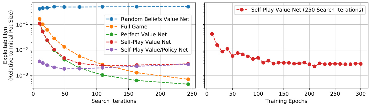
Figure 2: Convergence of different techniques in TEH. All subgames are solved using CFR-AVG. Perfect Value Net uses an oracle function to return the exact value of leaf nodes on each iteration. Self-Play Value Net uses a value function trained through self play. Self-Play Value/Policy Net additionally uses a policy network to warm start CFR. Random Beliefs trains the value net by sampling PBSs at random.

图 2: TEH中不同技术的收敛情况。所有子博弈均采用CFR-AVG求解。完美价值网络(Perfect Value Net)使用预言函数在每次迭代时返回叶节点的精确值。自博弈价值网络(Self-Play Value Net)采用通过自我对弈训练的价值函数。自博弈价值/策略网络(Self-Play Value/Policy Net)额外使用策略网络预热启动CFR。随机信念(Random Beliefs)通过随机采样PBSs训练价值网络。

Bot Name	Slumbot	BabyTartanian8 [9]	LBR [39]	Top Humans
DeepStack [40]			383± 112
Libratus [12]		63 ± 14		147 ± 39
Modicum [15]	11 ± 5	6±3
ReBeL (Ours)	45 ± 5	9±4	881 ± 94	165±69

Bot Name	Slumbot	BabyTartanian8 [9]	LBR [39]	Top Humans
DeepStack [40]			383± 112
Libratus [12]		63 ± 14		147 ± 39
Modicum [15]	11 ± 5	6±3
ReBeL (Ours)	45 ± 5	9±4	881 ± 94	165±69

Table 1: Head-to-head results of our agent against benchmark bots Baby Tartan ian 8 and Slumbot, as well as top human expert Dong Kim, measured in thousandths of a big blind per game. We also show performance against LBR [39] where the LBR agent must call for the first two betting rounds, and can either fold, call, bet $1\times$ pot, or bet all-in on the last two rounds. The $\pm$ shows one standard deviation. For Libratus, we list the score against all top humans in aggregate; Libratus beat Dong Kim by 29 with an estimated $\pm$ of 78.

表 1: 我们的AI智能体与基准机器人Baby Tartan ian 8、Slumbot以及人类顶尖专家Dong Kim的对战结果，以每局大盲注的千分之一为单位。我们还展示了与LBR [39] 的对战表现，其中LBR智能体在前两轮下注时必须跟注，后两轮可选择弃牌、跟注、下注1倍底池或全押。$\pm$ 表示一个标准差。对于Libratus，我们列出其对抗所有顶尖人类玩家的综合得分；Libratus以29分优势战胜Dong Kim，估计标准差为78。

Algorithm	1x4f	1x5f	1x6f	2x3f
Full-game FP	0.012	0.024	0.039	0.057
Full-game CFR	0.001	0.001	0.002	0.002
ReBeLFP	0.041	0.020	0.040	0.020
ReBeL CFR-D	0.017	0.015	0.024	0.017

算法	1x4f	1x5f	1x6f	2x3f
全游戏 FP	0.012	0.024	0.039	0.057
全游戏 CFR	0.001	0.001	0.002	0.002
ReBeLFP	0.041	0.020	0.040	0.020
ReBeL CFR-D	0.017	0.015	0.024	0.017

Table 2: Exploit ability of different algorithms of 4 variants of Liar’s Dice: 1 die with 4, 5, or 6 faces and 2 dice with 3 faces. The top two rows represent baseline numbers when a tabular version of the algorithms is run on the entire game for 1,024 iterations. The bottom 2 lines show the performance of ReBeL operating on subgames of depth 2 with 1,024 search iterations. For exploit ability computation of the bottom two rows, we averaged the policies of 1,024 play through s and thus the numbers are upper bounds on exploit ability.

表 2: 不同算法在4种变体骰子游戏(Liar's Dice)中的剥削能力：1颗4/5/6面骰和2颗3面骰。前两行表示算法在完整游戏上运行1,024次迭代时的基准数值。后两行显示ReBeL在深度为2的子游戏中运行1,024次搜索迭代的表现。计算后两行剥削能力时，我们平均了1,024次对局的策略，因此这些数值是剥削能力的上限。

9 Conclusions

9 结论

We present ReBeL, an algorithm that generalizes the paradigm of self-play reinforcement learning and search to imperfect-information games. We prove that ReBeL computes an approximate Nash equilibrium in two-player zero-sum games, demonstrate convergence in Liar’s Dice, and demonstrate that it produces superhuman performance in the benchmark game of heads-up no-limit Texas hold’em.

我们提出ReBeL算法，该算法将自我对弈强化学习和搜索范式推广至不完全信息博弈。我们证明ReBeL能在两人零和博弈中计算近似纳什均衡，在Liar's Dice游戏中展示收敛性，并在德州扑克单挑无限注基准测试中实现超越人类的表现。

ReBeL has some limitations that present avenues for future research. Most prominently, the input to its value and policy functions currently grows linearly with the number of infostates in a public state. This is intractable in games such as Recon Chess [44] that have strategic depth but very little common knowledge. ReBeL’s theoretical guarantees are also limited only to two-player zero-sum games.

ReBeL存在一些局限性，为未来研究提供了方向。最突出的是，其价值和策略函数的输入目前会随着公共状态中信息状态数量的增加而线性增长。这在诸如Recon Chess [44]等具有战略深度但共同知识极少的游戏中是难以处理的。此外，ReBeL的理论保证也仅限于两人零和游戏。

Nevertheless, ReBeL achieves low exploit ability in benchmark games and superhuman performance in heads-up no-limit Texas hold’em while leveraging far less expert knowledge than any prior bot. We view this as a major step toward developing universal techniques for multi-agent interactions.

然而，ReBeL在基准游戏中实现了较低的利用度，并在单挑无限注德州扑克中展现出超人类表现，同时比以往任何机器人都更少依赖专家知识。我们认为这是开发多智能体交互通用技术的重要一步。

Broader Impact

更广泛的影响

We believe ReBeL is a major step toward general equilibrium-finding algorithms that can be deployed in large-scale multi-agent settings while requiring relatively little domain knowledge. There are numerous potential future applications of this work, including auctions, negotiations, cyber security, and autonomous vehicle navigation, all of which are imperfect-information multi-agent interactions.

我们相信ReBeL是迈向通用均衡求解算法的重要一步，该算法可在需要较少领域知识的情况下部署于大规模多智能体场景。这项工作未来在拍卖、谈判、网络安全和自动驾驶导航等诸多不完美信息多智能体交互领域具有潜在应用前景。

The most immediate risk posed by this work is its potential for cheating in recreational games such as poker. While AI algorithms already exist that can achieve superhuman performance in poker, these algorithms generally assume that participants have a certain number of chips or use certain bet sizes. Retraining the algorithms to account for arbitrary chip stacks or unanticipated bet sizes requires more computation than is feasible in real time. However, ReBeL can compute a policy for arbitrary stack sizes and arbitrary bet sizes in seconds.

这项研究最直接的风险在于它可能在扑克等娱乐游戏中助长作弊行为。虽然现有AI算法已能在扑克游戏中实现超人类表现，但这些算法通常假设参与者拥有固定筹码量或采用特定下注规模。若需针对任意筹码量或意外下注规模重新训练算法，其计算量远超实时可行性。而ReBeL能在数秒内计算出适用于任意筹码量和任意下注规模的策略。

Partly for this reason, we have decided not to release the code for poker. We instead open source our implementation for Liar’s Dice, a recreational game that is not played as competitively by humans. The implementation in Liar’s Dice is also easier to understand and the size of Liar’s Dice can be more easily adjusted, which we believe makes the game more suitable as a domain for research.

部分出于这个原因，我们决定不发布扑克游戏的代码。相反，我们开源了骰子谎言(Liar's Dice)的实现，这是一款人类竞技性不强的休闲游戏。骰子谎言的实现更易于理解，且游戏规模可灵活调整，我们认为这使其更适合作为研究领域。

References

参考文献

A List of contributions

贡献列表

This paper makes several contributions, which we summarize here.

本文的主要贡献如下。

B Pseudocode for ReBeL

B ReBeL 伪代码

Algorithm 2 presents ReBeL in more detail.

算法 2 详细展示了 ReBeL。

We define the average of two policies to be the policy that is, in expectation, identical to picking one of the two policies and playing that policy for the entire game. Formally, if $\pi=\alpha\pi_{1}+(1-\alpha)\pi_{2}$ , then $\begin{array}{r}{\pi(s_{i})=\frac{\left(x_{i}^{\pi_{1}}(s_{i})\alpha\right)\pi_{1}(s_{i})+\left(x_{i}^{\pi_{2}}(s_{i})(1-\alpha)\right)\pi_{2}(s_{i})}{x_{i}^{\pi_{1}}(s_{i})\alpha+x_{i}^{\pi_{2}}(s_{i})(1-\alpha)}}\end{array}$ where $x_{i}^{\pi_{1}}(s_{i})$ is the product of the probabilities for all agent $i$ actions leading to $s_{i}$ . Formally, $x_{i}^{\pi}(s_{i})$ of infostate $s_{i}=(O_{i}^{0},a_{i}^{0},O_{i}^{1},a_{i}^{1},...,O_{i}^{t})$ is $x_{i}^{\pi}(s_{i}){\stackrel{.}{=}}\Pi_{t}(a_{i}^{t})$ .

我们将两种策略的平均值定义为：在期望意义上等同于从两种策略中随机选取一种，并在整个游戏中执行该策略的策略。形式上，若$\pi=\alpha\pi_{1}+(1-\alpha)\pi_{2}$，则$\begin{array}{r}{\pi(s_{i})=\frac{\left(x_{i}^{\pi_{1}}(s_{i})\alpha\right)\pi_{1}(s_{i})+\left(x_{i}^{\pi_{2}}(s_{i})(1-\alpha)\right)\pi_{2}(s_{i})}{x_{i}^{\pi_{1}}(s_{i})\alpha+x_{i}^{\pi_{2}}(s_{i})(1-\alpha)}}\end{array}$。其中$x_{i}^{\pi_{1}}(s_{i})$表示智能体$i$所有导致$s_{i}$状态的动作概率乘积。对于信息状态$s_{i}=(O_{i}^{0},a_{i}^{0},O_{i}^{1},a_{i}^{1},...,O_{i}^{t})$，其$x_{i}^{\pi}(s_{i})$可形式化表示为$x_{i}^{\pi}(s_{i}){\stackrel{.}{=}}\Pi_{t}(a_{i}^{t})$。

C Description of Games used for Evaluation

C 用于评估的游戏说明

C.1 Heads-up no-limit Texas hold’em poker (HUNL)

C.1 无限注德州扑克单挑赛 (HUNL)

HUNL is the two-player version of no-limit Texas hold’em poker, which is the most popular variant of poker in the world. For each “hand” (game) of poker, each player has some number of chips (the stack) in front of them. In our experiments, stack size varies during training between $\$5,000$ and $\$25,000$ but during testing is always $\$20,000$ , as is standard in the AI research community. Before play begins, Player 1 commits a small blind of $\$50$ to the pot and Player 2 commits a big blind of $\$100$ to the pot.

HUNL是无限制德州扑克的两人对战版本，这是全球最流行的扑克变体。每手牌局中，每位玩家面前都有一定数量的筹码（即记分牌）。在我们的实验中，训练阶段的筹码量在$\$5,000$到$\$25,000$之间浮动，但测试阶段固定为$\$20,000$，这是AI研究领域的标准设定。游戏开始前，玩家1需向底池投入小盲注$\$50$，玩家2需投入大盲注$\$100$。

lgorithm2ReBeL

function REBEL-LINEAR-CFR-D(βr,0",θ,D,D") > β is the current PBS while!IsTERMINAL(Br)do G ← CONSTRUCTSUBGAME(βr)

π, πtwam ←INITIALIZEPOLICY(G, 0") twarm = O and π° is uniform if no warm start G← SETLEAFVALUES(βr, πtwam , 0)

v(βr) < COMPUTEEV(G, πtwarm)

tsample ~ linear{twarm + 1, T} for t = (twarm + 1)..T do

if t = tsample then

β ← SAMPLELEAF(G, πt-1) > Sample one or multiple leaf PBSs πt UPDATEPOLICY(G,πt-1)

G SETLEAFVALUES(Br,πt,0")

u(βr)←u(βr)+ 2 COMPUTEEV(G, πt)

Add {βr,v(βr)} to Dv > Add to value net training data for β ∈G do > Loop over the PBS at every public state in G

Add {β, π(β)} to D" > Add to policy net training data (optional)

βr←βr

function SETLEAFVALUES(β, π, 0")

if IsLEAF(β) then for s E β do > For each infostate s corresponding to β v(si) =0(silβ,0)

算法2 ReBeL

function REBEL-LINEAR-CFR-D(βr,0",θ,D,D") > β为当前PBS
while!IsTERMINAL(Br)do
G ← CONSTRUCTSUBGAME(βr)
π, πtwam ←INITIALIZEPOLICY(G, 0") twarm = O且π°为均匀分布（若无热启动）
G← SETLEAFVALUES(βr, πtwam , 0)
v(βr) < COMPUTEEV(G, πtwarm)
tsample ~ linear{twarm + 1, T}
for t = (twarm + 1)..T do
if t = tsample then
β ← SAMPLELEAF(G, πt-1) > 采样一个或多个叶节点PBS
πt UPDATEPOLICY(G,πt-1)
G SETLEAFVALUES(Br,πt,0")
u(βr)←u(βr)+ 2 COMPUTEEV(G, πt)
将{βr,v(βr)}添加至Dv > 添加到价值网络训练数据
for β ∈G do > 遍历G中每个公共状态的PBS
将{β, π(β)}添加至D" > 添加到策略网络训练数据（可选）
βr←βr

function SETLEAFVALUES(β, π, 0")
if IsLEAF(β) then
for s E β do > 对于每个对应β的信息状态s
v(si) =0(silβ,0)

Once players commit their blinds, they receive two private cards from a standard 52-card deck. The first of four rounds of betting then occurs. On each round of betting, players take turns deciding whether to fold, call, or raise. If a player folds, the other player receives the money in the pot and the hand immediately ends. If a player calls, that player matches the opponent’s number of chips in the pot. If a player raises, that player adds more chips to the pot than the opponent. The initial raise of the round must be at least $\$100$ , and every subsequent raise on the round must be at least as large as the previous raise. A player cannot raise more than either player’s stack size. A round ends when both players have acted in the round and the most recent player to act has called. Player 1 acts first on the first round. On every subsequent round, player 2 acts first.

玩家下完盲注后，会从标准52张牌组中获得两张底牌。随后进行四轮下注中的第一轮。在每轮下注中，玩家轮流决定是否弃牌、跟注或加注。若玩家弃牌，对手将赢得底池筹码并立即结束当前牌局。若玩家跟注，则该玩家需匹配对手在底池中的筹码数。若玩家加注，则该玩家需投入比对手更多的筹码。首轮加注金额至少为$100，且同一轮后续每次加注金额不得低于前次加注额度。玩家加注金额不得超过任一玩家的剩余筹码量。当双方完成行动且最后行动方选择跟注时，该轮下注结束。第一轮由玩家1率先行动，后续每轮均由玩家2首先行动。

Upon completion of the first round of betting, three community cards are publicly revealed. Upon completion of the second betting round, another community card is revealed, and upon completion of the third betting round a final fifth community card is revealed. After the fourth betting round, if no player has folded, then the player with the best five-card poker hand, formed from the player’s two private cards and the five community cards, is the winner and takes the money in the pot. In case of a tie, the money is split.

第一轮下注结束后，公开亮出三张公共牌。第二轮下注结束后，再亮出一张公共牌；第三轮下注结束后，亮出最后第五张公共牌。第四轮下注后，若无人弃牌，则玩家用自己两张底牌与五张公共牌组成最优五张扑克牌组合，牌面最佳者赢得底池。若出现平局，则平分底池资金。

C.2 Turn endgame hold’em (TEH)

C.2 德州扑克终局对决 (TEH)

TEH is identical to HUNL except both players automatically call for the first two betting rounds, and there is an initial $\$1,000$ per player in the pot at the start of the third betting round. We randomize the stack sizes during training to be between $\$5,000$ and $\$50,000$ per player. The action space of TEH is reduced to at most three raise sizes $0.5\times$ pot, $1\times$ pot, or all-in for the first raise in a round, and $0.75\times$ pot or all-in for subsequent raises), but the raise sizes for non-all-in raises are randomly perturbed by up to $\pm0.1\times$ pot each game during training. Although we train on randomized stack sizes, bet sizes, and board cards, we measure exploit ability on the case of both players having $\$20,000$ , unperturbed bet sizes, and the first four board cards being $3667\bigcirc\mathrm{T}{\bigcirc}\mathrm{K}\pmb{\phi}$ . In this way we can train on a massive game while still measuring NashConv tractably. Even without the randomized stack and bet sizes, TEH has roughly $2\cdot10^{11}$ infostates.

TEH与HUNL完全相同，唯一的区别是前两轮下注阶段双方自动选择跟注，且在第三轮下注开始时每位玩家初始底池为$1,000。训练期间我们将每位玩家的筹码量随机设定在$5,000到$50,000之间。TEH的动作空间被缩减为每轮首次加注最多三种规模（0.5倍底池、1倍底池或全押），后续加注则为0.75倍底池或全押），但非全押加注的规模在训练期间每局会随机扰动±0.1倍底池。虽然训练时采用随机筹码量、下注规模和公共牌，但我们测量剥削性时设定双方筹码量均为$20,000、未扰动下注规模，且前四张公共牌为3667◯T◯K𝜙。通过这种方式，我们既能训练超大规模对局，又能有效计算NashConv。即使不采用随机筹码和下注规模，TEH仍包含约2·10¹¹个信息状态。

C.3 Liar’s Dice

C.3 骗子骰子

Liar’s Dice is a two-player zero-sum game in our experiments, though in general it can be played with more than two players. At the beginning of a game each player privately rolls $d$ dice with $f$ faces each. After that a betting stage starts where players take turns trying to predict how many dice of a specific kind there are among all the players, e.g., 4 dice with face 5. A player’s bid must either be for more dice than the previous player’s bid, or the same number of dice but a higher face. The round ends when a player challenges the previous bid (a call of liar). If all players together have at least as many dice of the specified face as was predicted by the last bid, then the player who made the bid wins. Otherwise the player who challenged the bid wins. We use the highest face as a wild face, i.e., dice with this face count towards a bid for any face.

在我们的实验中，诈唬骰子(Liar's Dice)是一个双人零和游戏，不过通常也可以多人参与。游戏开始时，每位玩家私下掷出$d$颗$f$面的骰子。随后进入叫分阶段，玩家轮流预测所有玩家骰子中特定点数的总数（例如4个5点骰）。玩家的叫分必须比前一位玩家叫的骰子数量更多，或骰子数量相同但点数更高。当有玩家质疑前一个叫分（即喊"诈唬"）时，回合结束。若所有玩家的骰子中确实存在至少与最后叫分相符的指定点数骰，则叫分者获胜；否则质疑者获胜。我们将最大点数设为万能骰，即该点数的骰子可计入任何点数的叫分。

D Domain Knowledge Leveraged in our Poker AI Agent

D 我们的扑克AI智能体所运用的领域知识

The most prominent form of domain knowledge in our ReBeL poker agent is the simplification of the action space during self play so that there are at most 8 actions at each decision point. The bet sizes are hand-chosen based on conventional poker wisdom and are fixed fractions of the pot, though each bet size is perturbed by $\pm0.1\times$ pot during training to ensure diversity in the training data.

在我们的ReBeL扑克AI智能体中，最突出的领域知识形式是在自我对弈期间简化动作空间，使每个决策点最多只有8个动作。下注量根据传统扑克策略手动选择，且固定为底池的特定比例，不过在训练期间每个下注量会以$\pm0.1\times$底池的幅度进行扰动，以确保训练数据的多样性。

We specifically chose not to leverage domain knowledge that has been widely used in previous poker AI agents:

我们特意选择不利用先前扑克AI智能体中广泛使用的领域知识：

• All prior top poker agents, including DeepStack [40], Libratus [12], and Pluribus [14], have used information abstraction to bucket similar infostates together based on domain-specific features [30, 21, 6]. Even when computing an exact policy, such as during search or when solving a poker game in its entirety [24, 4], past agents have used lossless abstraction in which strategically identical infostates are bucketed together. For example, a flush of spades may be strategically identical to a flush of hearts. Our agent does not use any information abstraction, whether lossy or lossless. The agent computes a unique policy for each infostate. The agent’s input to its value and policy

• 所有先前的顶级扑克AI智能体，包括DeepStack [40]、Libratus [12]和Pluribus [14]，都使用信息抽象（information abstraction）技术，基于领域特定特征将相似的信息状态（infostates）分组处理 [30, 21, 6]。即便在计算精确策略时（例如在搜索过程中或完整求解扑克游戏时 [24, 4]），过往的AI智能体也采用无损抽象（lossless abstraction）方式，将策略上完全等同的信息状态归为一组。例如，黑桃同花可能与红桃同花在策略上是完全相同的。我们的AI智能体不使用任何形式的信息抽象（无论是有损还是无损），而是为每个信息状态计算独立策略。该智能体对其价值和策略网络的输入...

E Hyper parameters

E 超参数

In this section we provide details of the value and policy networks and the training procedures.

在本节中，我们将详细介绍价值网络 (value network) 和策略网络 (policy network) 的结构及训练流程。

We approximate the value and policy functions using artificial neural networks. The input to the value network consists of three components for both games: agent index, representation of the public state, and a probability distribution over infostates for both agents. For poker, the public state representation consists of the board cards and the common pot size divided by stack size; for Liar’s Dice it is the last bid and the acting agent. The output of the network is a vector of values for each possible infostate of the indexed agent, e.g., each possible poker hand she can hold.

我们使用人工神经网络来近似价值函数和策略函数。价值网络的输入包含三个组成部分（适用于两种游戏）：智能体索引、公共状态表示以及两个智能体的信息状态概率分布。对于扑克游戏，公共状态表示由公共牌和底池大小除以筹码量构成；对于骗子骰游戏，则是最近一次叫价和当前行动智能体。网络输出是一个向量，表示索引智能体每个可能信息状态的价值，例如她可能持有的每一手扑克牌。

We trained a policy network only for poker. The policy network state representation additionally contains pot size fractions for both agents separately as well as a flag for whether there have been any bets so far in the round. The output is a probability distribution over the legal actions for each infostate.

我们训练了一个仅针对扑克的策略网络。该策略网络的状态表示额外包含两个智能体各自的底池大小比例，以及一个标志位用于表示当前回合是否已有下注行为。输出结果是针对每个信息状态下合法动作的概率分布。

As explained in section 7 we use Multilayer perceptron with GeLU [27] activation functions and LayerNorm [3] for both value and policy networks.

如第7节所述，我们在价值和策略网络中均采用带GeLU [27]激活函数的多层感知机及LayerNorm [3]。

For poker we represent the public state as a concatenation of a vector of indices of the board cards, current pot size relative to the stack sizes, and binary flag for the acting player. The size of the full input is

在扑克游戏中，我们将公共状态表示为以下内容的拼接：桌面牌索引向量、当前底池大小相对于筹码堆大小的比例，以及行动玩家的二进制标志位。完整输入的大小为

$$
[1(\text{agent index}) + 1(\text{acting agent}) + 1(\text{pot}) + 5(\text{board}) + 2 \times 1326(\text{infostate beliefs})]
$$

We use card embedding for the board cards similar to [7] and then apply MLP. Both the value and the policy networks contain 6 hidden layers with 1536 layers each. For all experiments we set the probability to explore a random action to $\epsilon=25%$ (see Section 5.2). To store the training data we use a simple circular buffer of size 12M and sample uniformly. Since our action abstraction contains at most 9 legal actions, the size of the target vector for the policy network is 9 times bigger than one used for the value network. In order to make it manageable, we apply linear quantization to the policy values. As initial data is produced with a random value network, we remove half of the data from the replay buffer after 20 epochs.

我们采用类似[7]的方法对公共牌进行卡牌嵌入(card embedding)，然后应用多层感知机(MLP)。价值网络和策略网络均包含6个隐藏层，每层1536个神经元。所有实验中，我们将随机探索动作的概率设置为$\epsilon=25%$(参见5.2节)。训练数据存储采用容量为1200万的简单循环缓冲区，并进行均匀采样。由于我们的动作抽象最多包含9个合法动作，策略网络的目标向量尺寸是价值网络的9倍。为便于处理，我们对策略值采用线性量化。由于初始数据由随机价值网络生成，我们在20个训练周期后从回放缓冲区移除了半数数据。

For the full game we train the network with Adam optimizer with learning rate $3\times10^{-4}$ and halved the learning rate every 800 epochs. One epoch is 2,560,000 examples and the batch size 1024. We used 90 DGX-1 machines, each with $8\times32\mathrm{GB}$ Nvidia V100 GPUs for data generation. We report results after 1,750 epochs. For TEH experiments we use higher initial learning rate $4\times10^{-4}$ , but halve it every 100 epochs. We report results after 300 epochs.

在完整游戏中，我们使用学习率为 $3\times10^{-4}$ 的Adam优化器训练网络，并每800个周期将学习率减半。每个周期包含2,560,000个样本，批次大小为1024。数据生成阶段使用了90台DGX-1机器，每台配备 $8\times32\mathrm{GB}$ 的Nvidia V100 GPU。最终结果在1,750个周期后汇报。针对TEH实验，我们采用更高的初始学习率 $4\times10^{-4}$ ，但每100个周期减半一次。实验结果在300个周期后汇报。

For Liar’s Dice we represent the state as a concatenation of a one hot vector for the last bid and binary flag for the acting player. The size of the full input is

在《骗子骰》游戏中，我们将状态表示为最后叫骰点数的独热编码向量与当前行动玩家二进制标志的连接。完整输入的尺寸为

$$
[1(\text{agent index}) + 1(\text{acting agent}) + n_{\text{dice}}n_{\text{faces}}(\text{last bid}) + 2n_{\text{faces}}n_{\text{dice}}(\text{infostate beliefs})]
$$

The value network contains 2 hidden layers with 256 layers each. We train the network with Adam optimizer with learning rate $3\times10^{-4}$ and halved the learning rate every 400 epochs. One epoch is 25,600 examples and the batch size 512. During both training and evaluation we run the search algorithm for 1024 iterations. We use single GPU for training and 60 CPU threads for data generation. We trained the network for 1000 epochs. To reduce the variance in RL $^+$ Search results, we evaluated the three last checkpoints and reported averages in table 2.

价值网络包含2个隐藏层，每层256个节点。我们使用学习率为 $3\times10^{-4}$ 的Adam优化器进行训练，并每400个周期将学习率减半。每个周期包含25,600个样本，批次大小为512。在训练和评估阶段，我们都运行1024次搜索算法迭代。训练使用单块GPU，数据生成使用60个CPU线程。网络共训练了1000个周期。为降低RL$^+$搜索结果的方差，我们评估了最后三个检查点并在表2中报告了平均值。

E.1 Human Experiments for HUNL

E.1 无限注德州扑克人类实验

We evaluated our HUNL agent against Dong Kim, a top human professional specializing in HUNL. Kim was one of four humans that played against Libratus [12] in the man-machine competition which Libratus won. Kim lost the least to Libratus. However, due to high variance, it is impossible to statistically compare the performance of the individual humans that participated in the competition.

我们让HUNL智能体与专攻HUNL的顶尖人类职业选手Dong Kim进行了对抗测试。Kim曾是人机大战中对抗Libratus [12] 的四位人类选手之一（该比赛以Libratus获胜告终）。Kim是当时对阵Libratus时输分最少的选手。但由于方差过高，无法从统计学角度比较参赛选手间的个体表现差异。

A total of 7,500 hands were played between Kim and the bot. Kim was able to play from home at his own pace on any schedule he wanted. He was also able to play up to four games simultaneously against the bot. To in centi viz e strong play, Kim was offered a base compensation of $\$1\pm\S0.05x$ for each hand played, where $x$ signifies his average win/loss rate in terms of big blinds per hundred hands played. Kim was guaranteed a minimum of $\$0.75$ per hand and could earn no more than $\text{\$2}$ per hand. Since final compensation was based on the variance-reduced score rather than the raw score, Kim was not aware of his precise performance during the experiment.

Kim与机器人总共进行了7500手牌局。Kim可以在家中按自己的节奏自由安排时间进行游戏，还能同时与机器人进行最多四局对战。为了激励高水平发挥，Kim每完成一手牌可获得基础报酬 $\$1\pm\S0.05x$ ，其中 $x$ 代表其每百手牌的大盲注盈亏率。保底报酬为每手 $\$0.75$ ，上限为每手 $\text{\$2}$ 。由于最终报酬基于方差缩减分数而非原始分数，Kim在实验期间无法知晓自己的精确表现。

The bot played at an extremely fast pace. No decision required more than 5 seconds, and the bot on average plays faster than 2 seconds per hand in self play. To speed up play even further, the bot cached subgames it encountered on the preflop. When the same subgame was encountered again, it would simply reuse the solution it had already computed previously.

该AI以极快的速度进行游戏。每个决策耗时不超过5秒，在自我对弈中平均每手牌仅需不到2秒。为了进一步加速游戏进程，AI会缓存遇到的翻牌前子游戏(subgame)。当再次遇到相同子游戏时，它直接复用之前计算好的解决方案。

Kim’s variance-reduced score, which we report in Section 8, was a loss of $165\pm69$ where the $\pm$ indicates one standard error. His raw score was a loss of $358\pm188$ .

Kim的方差缩减得分（我们将在第8节报告）为损失 $165\pm69$，其中 $\pm$ 表示一个标准误差。他的原始得分为损失 $358\pm188$。

F 与价值函数相关的证明（定理 1）

We start by proving some preliminary Lemmas. For simplicity, we will sometimes prove results for only one player, but the results hold WLOG for both players.

我们首先证明一些预备引理。为简化起见，有时仅针对单方玩家进行证明，但根据对称性 (WLOG) 结论对双方玩家均成立。

For some policy profile $\pi=(\pi_{1},\pi_{2})$ , let $v_{i}^{\pi}(\beta):B\rightarrow\mathbb{R}^{|S_{i}|}$ be a function that takes as input a PBS and outputs infostate values for player $i$ .

对于某些策略组合 $\pi=(\pi_{1},\pi_{2})$，设 $v_{i}^{\pi}(\beta):B\rightarrow\mathbb{R}^{|S_{i}|}$ 为一个函数，该函数以 PBS 为输入并输出玩家 $i$ 的信息状态值。

Proof. This follows directly from the definition of $v_{i}^{\pi}(s_{i}|\beta)$ along with the definition of $V_{1}$ ,

证明。这直接源于$v_{i}^{\pi}(s_{i}|\beta)$的定义以及$V_{1}$的定义。

$$
V_{1}^{\pi_{2}}(\beta)=\sum_{s_{1}\in S_{1}(s_{\mathrm{pub}})}\beta_{1}(s_{1})v_{1}(s_{1}|\beta,(B R(\pi_{2}),\pi_{2}))
$$

Lemma 2. $\begin{array}{r}{V_{1}(\beta)=\operatorname*{min}_ {\pi_{2}}V_{1}^{\pi_{2}}(\beta)}\end{array}$ , and the set of $\pi_{2}$ that attain $V_{1}(\beta)$ at $\beta_{0}$ are precisely the Nash equilibrium policies at $\beta_{0}$ . This also implies that $V_{1}(\beta)$ is concave.

引理 2. $\begin{array}{r}{V_{1}(\beta)=\operatorname*{min}_ {\pi_{2}}V_{1}^{\pi_{2}}(\beta)}\end{array}$，且在 $\beta_{0}$ 处达到 $V_{1}(\beta)$ 的 $\pi_{2}$ 策略集合恰好是 $\beta_{0}$ 处的纳什均衡策略。这也意味着 $V_{1}(\beta)$ 是凹函数。

Proof. By definition, the Nash equilibrium at $\beta$ is the minimum among all choices of $\pi_{2}$ of the value to player 1 of her best response to $\pi_{2}$ . Any $\pi_{2}$ that achieves this Nash equilibrium value when playing a best response is a Nash equilibrium policy.

证明。根据定义，在$\beta$处的纳什均衡是玩家1对所有$\pi_{2}$选择的最佳响应值中的最小值。任何在最佳响应时达到该纳什均衡值的$\pi_{2}$即为纳什均衡策略。

From Lemma 1, we know that each $V_{1}^{\pi_{2}}(\beta)$ is linear, which implies that $V_{1}(\beta)$ is concave since any function that is the minimum of linear functions is concave. 口

根据引理1，我们知道每个$V_{1}^{\pi_{2}}(\beta)$都是线性的，这意味着$V_{1}(\beta)$是凹函数，因为任何作为线性函数最小值的函数都是凹的。口

Figure 3: Illustration of Lemma 2. In this simple example, the subgame begins with some probability $\beta(h e a d s)$ of a coin being heads-up, which player 1 observes. Player 2 then guesses if the coin is heads or tails, and wins if he guesses correctly. The payoffs for Player 2’s pure strategies are shown as the lines marked $\pi_{2}^{h e a d s}$ and $\pi_{2}^{t a i l s}$ . The payoffs for a mixed strategy is a linear combination of the pure strategies. The value for player 1 is the minimum among all the lines corresponding to player 2 strategies, denoted by the solid lines.

图 3: 引理2的图示。在这个简单示例中，子博弈开始时硬币正面朝上的概率为$\beta(h e a d s)$，玩家1观察到该信息。玩家2随后猜测硬币是正面还是反面，猜对即获胜。玩家2纯策略的收益用标记为$\pi_{2}^{h e a d s}$和$\pi_{2}^{t a i l s}$的线条表示。混合策略的收益是纯策略的线性组合。玩家1的收益值是对应于玩家2所有策略线条中的最小值，用实线表示。

Now we can turn to proving the Theorem.

现在我们可以着手证明该定理。

Consider a function $\tilde{V}_ {1}$ that is an extension of $V_{1}$ to un normalized probability distributions over $S_{1}$ and $S_{2}$ ; i.e. $\tilde{V}_ {i}((s_{p u b},b_{1},b_{2}))=V_{i}((s_{\mathrm{pub}},b_{1}/|b_{1}|_ {1},b_{2}/|b_{2}|_ {1}))$ . $\tilde{V}_ {i}=V_{i}$ on the simplex of valid beliefs, but we extend it in this way to $\mathbb{R}_ {\geq0}^{|s_{1}|}\setminus\vec{0}$ so that we can consider gradients w.r.t. $p(s_{1})$ .

考虑一个函数 $\tilde{V}_ {1}$，它是 $V_{1}$ 对 $S_{1}$ 和 $S_{2}$ 上非归一化概率分布的扩展；即 $\tilde{V}_ {i}((s_{p u b},b_{1},b_{2}))=V_{i}((s_{\mathrm{pub}},b_{1}/|b_{1}|_ {1},b_{2}/|b_{2}|_ {1}))$。在有效信念的单纯形上 $\tilde{V}_ {i}=V_{i}$，但我们以这种方式将其扩展到 $\mathbb{R}_ {\geq0}^{|s_{1}|}\setminus\vec{0}$，以便考虑关于 $p(s_{1})$ 的梯度。

We will use the term ‘super gradient’ to be the equivalent of the sub gradient for concave functions. Formally, $g$ is a super gradient of concave function $F$ at $x_{0}$ iff for any $x$ in the domain of $F$ ,

我们将用“超梯度 (super gradient)”这一术语来表示凹函数的次梯度等价概念。形式上，$g$ 是凹函数 $F$ 在 $x_{0}$ 处的超梯度，当且仅当对于 $F$ 定义域内的任意 $x$，

$$
F(x)-F(x_{0})\leq g\cdot(x-x_{0}).
$$

Also, $s u p e r g(F)=-s u b g(-F)$ .

此外，$s u p e r g(F)=-s u b g(-F)$。

Theorem (Restatement of Theorem 1). For any belief $\beta=(\beta_{1},\beta_{2})$ (for the beliefs over player 1 and 2 infostates respectively) and any policy $\pi^{*}$ that is a Nash equilibrium of the subgame rooted at $\beta$ ,

定理 (定理1重述). 对于任意信念 $\beta=(\beta_{1},\beta_{2})$ (分别表示玩家1和玩家2信息状态的信念) 以及任意在 $\beta$ 为根的子博弈中构成纳什均衡的策略 $\pi^{*}$ ,

$$
v_{1}^{\pi^{*}}(s_{1}|\beta)=V_{1}(\beta)+\bar{g}\cdot\hat{s}_{1}
$$

for some super gradient $\bar{g}$ of $\tilde{V}_ {1}(\beta)$ with respect to $\beta_{1}$ , where $\hat{s}_ {1}$ is the unit vector in direction $s_{1}$

对于 $\tilde{V}_ {1}(\beta)$ 关于 $\beta_{1}$ 的某个超梯度 $\bar{g}$ ，其中 $\hat{s}_ {1}$ 是方向 $s_{1}$ 上的单位向量

Proof. Lemma 2 shows that $V_{1}(\beta)$ is a concave function in $\beta_{1}$ , and its extension $\tilde{V}$ off the simplex is constant perpendicular to the simplex, so $\tilde{V}$ is concave as well. Therefore the notion of a super gradient is well-defined.

证明。引理 2 表明 $V_{1}(\beta)$ 是 $\beta_{1}$ 的凹函数，其在单纯形外的扩展 $\tilde{V}$ 垂直于单纯形方向为常数，因此 $\tilde{V}$ 也是凹函数。故超梯度概念是良定义的。

Now, consider some policy profile $\pi^{ * }=(\pi_{1}^{ * },\pi_{2}^{ * })$ that is a Nash equilibrium of $G(\beta_{0}).:V_{1}^{\pi_{2}^{*}}$ is a linear function and tangent to $V_{1}$ at $\beta_{0}$ ; therefore, its gradient is a super gradient of $V_{1}$ at $\beta_{0}$ . Its gradient is

现在考虑某个策略组合 $\pi^{ * }=(\pi_{1}^{ * },\pi_{2}^{ * })$ ，它是 $G(\beta_{0})$ 的纳什均衡。 $V_{1}^{\pi_{2}^{*}}$ 是一个线性函数，且在 $\beta_{0}$ 处与 $V_{1}$ 相切；因此，它的梯度是 $V_{1}$ 在 $\beta_{0}$ 处的超梯度。其梯度为

$$
\begin{array}{c l}{{\displaystyle\nabla_{\beta_{1}}V_{1}^{\pi^{ * }}(\beta)=\nabla_{\beta_{1}}\sum_{s_{1}\in S_{1}(s_{\mathrm{pub}})}\beta_{1}(s_{1}){v_{1}^{\pi^{ * }}}_ {}(s_{1}|\beta)}}\ {{\displaystyle=\sum_{s_{1}\in S_{1}(s_{\mathrm{pub}})}\hat{s}_ {1}{v_{1}^{\pi^{ * }}}_ {}(s_{1}|\beta)+\beta(s_{1})\nabla_{\beta_{1}}{v^{\pi^{ * }}}_ {}(s_{1}|\beta)}}\ {{\displaystyle=\sum_{s_{1}\in S_{1}(s_{\mathrm{pub}})}\hat{s}_ {1}{v_{1}^{\pi^{*}}}_ {}(s_{1}|\beta)}}\end{array}
$$

Equation 6 follows from the fact that for a fixed opponent policy $\pi_{2}^{ * }$ , each player 1 infostate $s_{1}$ is an independent MDP whose value $v_{1}^{\pi_{2}^{*}}(s_{1}|\beta)$ doesn’t depend on the probabilities $\beta_{1}$ of being in the different infostates (although it might depend on $\beta_{2}$ since player 1 doesn’t observe these).

式6成立的原因在于，对于固定的对手策略$\pi_{2}^{ * }$，玩家1的每个信息状态$s_{1}$都是一个独立的马尔可夫决策过程(MDP)，其值函数$v_{1}^{\pi_{2}^{*}}(s_{1}|\beta)$不依赖于处于不同信息状态的概率$\beta_{1}$（尽管它可能依赖于$\beta_{2}$，因为玩家1无法观测到这些信息）。

Note also that the gradient of $V_{1}^{\pi_{2}^{ * }}$ is correct even when some infostates $s_{1}$ have probability 0, due to the fact that we defined $v_{1}^{\pi_{2}}(s_{1}|\beta)$ as the value of player 1 playing a best response to $\pi_{2}$ at each infostate $s_{1}$ (rather than just playing the equilibrium policy $\pi_{1}^{*}$ , which may play arbitrarily at unvisited infostates).

还需注意的是，即使某些信息状态 $s_{1}$ 的概率为0，$V_{1}^{\pi_{2}^{ * }}$ 的梯度仍然是正确的。这是因为我们将 $v_{1}^{\pi_{2}}(s_{1}|\beta)$ 定义为玩家1在每个信息状态 $s_{1}$ 下对 $\pi_{2}$ 采取最佳响应(而非仅遵循均衡策略 $\pi_{1}^{*}$ ——该策略可能在未访问的信息状态下任意行动)时的价值。

Finally, let’s compute $g\cdot\hat{s}_ {1}$ at some $\beta_{1}$ on the simplex (i.e. $|\beta_{1}|_{1}=1;$ ).

最后，我们在单纯形上的某个 $\beta_{1}$ 处（即 $|\beta_{1}|_ {1}=1;$ ）计算 $g\cdot\hat{s}_{1}$。

我们完成了。

G 子博弈求解相关证明 (定理 2 和 3)

Lemma 3. Running Algorithm 1 for $N\rightarrow\infty$ times in a depth-limited subgame rooted at PBS $\beta_{r}$ will compute an infostate value vector $v_{i}^{\pi^{ * }}(\beta_{r})$ corresponding to the values of the infostates when $\pi^{ * }$ is played in the (not depth-limited) subgame rooted at $\beta_{r}$ , where $\pi^{*}$ is a √CT -Nash equilibrium for some constant $C$ .

引理 3. 在根节点为PBS $\beta_{r}$ 的深度受限子博弈中运行算法1 $N\rightarrow\infty$ 次，将计算出信息状态值向量 $v_{i}^{\pi^{ * }}(\beta_{r})$ ，该向量对应于在根节点为 $\beta_{r}$ 的(非深度受限)子博弈中执行策略 $\pi^{ * }$ 时的信息状态值。其中 $\pi^{*}$ 是某个常数 $C$ 对应的√CT -纳什均衡策略。

Proof. A key part of our proof is the insight that Algorithm 1 resembles the CFR-D algorithm from [16] if Algorithm 1 were modified such that there was no random sampling and every call to the value network was replaced with a recursive call to the CFR-D algorithm.

证明。我们证明的一个关键部分在于认识到，如果对算法1进行修改，使其不进行随机采样，并将每次对价值网络的调用替换为对CFR-D算法的递归调用，那么算法1就类似于[16]中的CFR-D算法。

Suppose the subgame rooted at $\beta_{r}$ extends to the end of the game and therefore there are no calls to the neural network. Then CFR is proven to compute a $\frac{C}{\sqrt{T}}$ -Nash equilibrium [61], which we will call $\pi^{ * }$ , and Algorithm 1 will indeed learn a value vector $v_{i}^{\pi^{ * }}(\beta_{r})$ for $\beta_{r}$ corresponding to the infostate values of $\beta_{r}$ when $\pi^{*}$ is played in the subgame. Thus, the base case for the inductive proof holds.

假设以$\beta_{r}$为根的子博弈延续到游戏结束且不调用神经网络。根据证明[61]，CFR能够计算出$\frac{C}{\sqrt{T}}$纳什均衡（记作$\pi^{ * }$），此时算法1确实会学习到一个价值向量$v_{i}^{\pi^{ * }}(\beta_{r})$，该向量对应于当$\pi^{*}$在子博弈中执行时$\beta_{r}$的信息状态值。因此，归纳证明的基准情况成立。

Now suppose we have a depth-limited subgame rooted at $\beta_{r}$ . Assume that for every leaf PBS ${\beta_{z}^{\pi}}^{t}$ for iterations $t\leq T$ , where $\pi^{t}$ is the policy in the subgame on iteration $t$ , that we have already computed an infostate value vector $v_{i}^{\pi^{ * }}(\beta_{z}^{\pi^{t}})$ corresponding to the values of the infostates in ${\beta_{z}^{\pi}}^{t}$ when $\pi^{ * }$ is played in the subgame rooted at $\beta_{z}^{\pi^{t}}$ , where $\pi^{*}$ is a $\frac{C}{\sqrt{T}}$ -Nash equilibrium for some constant $C$ . Assume also that Lemma 3 holds for all leaf PBSs βzπT +1.

现在假设我们有一个以 $\beta_{r}$ 为根的深度受限子博弈。假设对于每次迭代 $t\leq T$ 的叶节点 PBS ${\beta_{z}^{\pi}}^{t}$ (其中 $\pi^{t}$ 是第 $t$ 次迭代时子博弈的策略)，我们已经计算出了一个信息状态值向量 $v_{i}^{\pi^{ * }}(\beta_{z}^{\pi^{t}})$，该向量对应 ${\beta_{z}^{\pi}}^{t}$ 中信息状态在以 $\beta_{z}^{\pi^{t}}$ 为根的子博弈中采用 $\pi^{ * }$ 策略时的值，其中 $\pi^{*}$ 是某个常数 $C$ 对应的 $\frac{C}{\sqrt{T}}$ -纳什均衡。同时假设引理3对所有叶节点 PBS $\beta_{z}^{\pi^{T +1}}$ 都成立。

First, for leaf PBSs that neither player reaches with positive probability, the values for the leaf PBS have no affect on CFR or the values computed for the root infostates because CFR weights the values by the probability the player reaches the PBS [61].

首先，对于双方玩家到达概率均为零的叶节点 PBS (Public Belief State)，其取值不会影响 CFR (Counterfactual Regret Minimization) 或根信息状态的估值计算，因为 CFR 会通过玩家到达 PBS 的概率对估值进行加权 [61]。

Now consider a leaf PBS $\beta_{z}^{\pi^{T+1}}$ that some player reaches with positive probability. Since $v_{i}^{\pi^{ * }}(\beta_{z}^{\pi^{t}})$ has already been computed for all $\beta_{z}^{\pi^{t}}$ and since we are running a deterministic algorithm, so $v_{i}^{\pi^{ * }}(\beta_{z}^{\pi^{t}})$ will not change with subsequent calls of Algorithm 1 on $\beta_{z}^{\pi^{t}}$ for all $t\leq T$ . Thus, $\pi^{t}$ will be the same for all $t\leq T$ . Since Algorithm 1 samples a random CFR iteration, and since the leaf PBS $\beta_{z}^{\pi^{T+1}}$ is sampled with positive probability for some player when iteration $T+1$ is sampled, so the algorithm will sample $\bar{\beta_{z}^{\pi^{T+1}}}N^{j}$ times, where $N^{\prime}\to\infty$ as $N\rightarrow\infty$ . Since Lemma 3 holds for $\beta_{z}^{\pi^{\bar{T}+1}}$ , so eventually $v_{i}^{\pi^{*}}(\beta_{z}^{\pi^{T+1}})$ will be computed for $\beta_{z}^{\pi^{T+1}}$ . Therefore, due to CFR-D [16], Lemma 3 will hold for $\beta_{r}$ and the inductive step is proven. 口

现在考虑某个玩家以正概率到达的叶节点 PBS $\beta_{z}^{\pi^{T+1}}$。由于对于所有 $\beta_{z}^{\pi^{t}}$ 的 $v_{i}^{\pi^{ * }}(\beta_{z}^{\pi^{t}})$ 已经计算完成，并且我们运行的是确定性算法，因此对于所有 $t\leq T$，后续在 $\beta_{z}^{\pi^{t}}$ 上调用算法 1 时 $v_{i}^{\pi^{ * }}(\beta_{z}^{\pi^{t}})$ 不会改变。因此，对于所有 $t\leq T$，$\pi^{t}$ 将保持不变。由于算法 1 随机采样一个 CFR 迭代，并且当采样到迭代 $T+1$ 时，叶节点 PBS $\beta_{z}^{\pi^{T+1}}$ 对某个玩家以正概率被采样，因此算法将采样 $\bar{\beta_{z}^{\pi^{T+1}}}N^{j}$ 次，其中 $N^{\prime}\to\infty$ 当 $N\rightarrow\infty$ 时。由于引理 3 对 $\beta_{z}^{\pi^{\bar{T}+1}}$ 成立，因此最终会为 $\beta_{z}^{\pi^{T+1}}$ 计算出 $v_{i}^{\pi^{*}}(\beta_{z}^{\pi^{T+1}})$。因此，根据 CFR-D [16]，引理 3 对 $\beta_{r}$ 成立，归纳步骤得证。口

Theorem (Restatement of Theorem 2). Consider an idealized value approx im at or that returns the most recent sample of the value for sampled PBSs, and 0 otherwise. Running Algorithm $I$ with $T$ iterations of CFR in each subgame will produce a value approx im at or that produces values that correspond to a √CT -equilibrium policy for any PBS that could be encountered during play, where C is a game-dependent constant.

定理 (定理2重述). 考虑一个理想化的价值近似器，该近似器对采样的PBS返回其最新样本值，否则返回0。在每个子游戏中运行CFR算法 $I$ 次迭代，共进行 $T$ 次迭代，将产生一个价值近似器。对于游戏过程中可能遇到的任何PBS，该近似器产生的值对应于√CT均衡策略，其中C是一个与游戏相关的常数。

Proof. Since we run Algorithm 1 for $N\rightarrow\infty$ times at the root of the game, so by Lemma 3, Theorem 2 is true. 口

证明。由于我们在游戏根节点处运行算法1 $N\rightarrow\infty$ 次，因此根据引理3，定理2成立。口

Theorem (Restatement of Theorem 3). If Algorithm 1 is run at test time with no off-policy exploration, a value network that has error at most $\delta$ for any leaf PBS, and with $T$ iterations of CFR being used to solve subgames, then the algorithm plays $a$ $\begin{array}{r}{(\delta\dot{C}_ {1}+\frac{\delta C_{2}}{\sqrt{T}})}\end{array}$ -Nash equilibrium, where $C_{1},C_{2}$ are game-specific constants.

定理 (定理3重述). 如果在测试时运行算法1时不进行离策略探索, 且对于任何叶节点PBS值网络的误差最多为$\delta$, 同时使用$T$次CFR迭代求解子博弈, 则该算法将达成$a$ $\begin{array}{r}{(\delta\dot{C}_ {1}+\frac{\delta C_{2}}{\sqrt{T}})}\end{array}$-纳什均衡, 其中$C_{1},C_{2}$为博弈特定常数。

Proof. We prove the theorem inductively. Consider first a subgame near the end of the game that is not depth-limited. I.e., it has no leaf nodes. Clearly, the policy $\pi^{*}$ that Algorithm 1 using CFR plays in expectation is a $\frac{k_{1}}{\sqrt{T}}$ -Nash equilibrium for game-specific constant $k_{1}$ in this subgame.

证明。我们通过归纳法证明该定理。首先考虑一个接近游戏末尾且不受深度限制的子游戏，即该子游戏没有叶节点。显然，算法1使用反事实遗憾最小化(CFR)策略$\pi^{*}$在该子游戏中以期望方式达到特定游戏常数$k_{1}$的$\frac{k_{1}}{\sqrt{T}}$ -纳什均衡。

Rather than play the average policy over all $T$ iterations $\bar{\pi}^{T}$ , one can equivalently pick a random iteration $t\sim\mathrm{uniform}{1,T}$ and play according to $\pi^{t}$ , the policy on iteration $t$ . This algorithm is also a $\frac{k_{1}}{\sqrt{T}}$ -Nash equilibrium in expectation.

与在所有$T$次迭代中执行平均策略$\bar{\pi}^{T}$不同，可以等效地随机选择一个迭代$t\sim\mathrm{uniform}{1,T}$并执行该次迭代的策略$\pi^{t}$。该算法在期望意义上同样是一个$\frac{k_{1}}{\sqrt{T}}$-纳什均衡。

Next, consider a depth-limited subgame $G$ such that for any leaf PBS $\beta^{t}$ on any CFR iteration $t$ , the policy that Algorithm 1 plays in the subgame rooted at $\beta^{t}$ is in expectation a $\delta$ -Nash equilibrium in the subgame. If one computes a policy for $G$ using tabular CFR-D [16] (or, as discussed in Section I, using CFR-AVG), then by Theorem 2 in [16], the average policy over all iterations is $k_{2}\delta+\frac{k_{3}}{\sqrt{T}}$ -Nash equilibrium.

接下来，考虑一个深度受限的子博弈 $G$，使得对于任何 CFR 迭代 $t$ 上的任意叶节点 PBS $\beta^{t}$，算法 1 在以 $\beta^{t}$ 为根的子博弈中执行的策略在期望上是一个 $\delta$-纳什均衡。如果使用表格化 CFR-D [16] (或如第一节所述，使用 CFR-AVG) 为 $G$ 计算策略，那么根据 [16] 中的定理 2，所有迭代的平均策略是一个 $k_{2}\delta+\frac{k_{3}}{\sqrt{T}}$-纳什均衡。

Just as before, rather than play according to this average policy $\bar{\pi}^{T}$ , one can equivalently pick a random iteration $t\sim\mathrm{uniform}{1,T}$ and play according to $\pi^{t}$ . Doing so would also result in a $\begin{array}{r}{k_{2}\delta+\frac{k_{3}}{\sqrt{T}}}\end{array}$ -Nash equilibrium in expectation. This is exactly what Algorithm 1 does.

与之前一样，与其按照这个平均策略 $\bar{\pi}^{T}$ 行动，可以等价地随机选择一个迭代 $t\sim\mathrm{uniform}{1,T}$ 并按照 $\pi^{t}$ 行动。这样做同样会在期望中得到一个 $\begin{array}{r}{k_{2}\delta+\frac{k_{3}}{\sqrt{T}}}\end{array}$ -纳什均衡。这正是算法1所实现的。

Since there are a finite number of “levels” in a game, which is a game-specific constant, Algorithm 1 plays according to a $\begin{array}{r}{\delta C_{1}+\frac{\delta C_{2}}{\sqrt{T}}}\end{array}$ δ√C2 -Nash equilibrium.

由于游戏中存在有限数量的"关卡"，这是一个游戏特定的常数，算法1按照$\begin{array}{r}{\delta C_{1}+\frac{\delta C_{2}}{\sqrt{T}}}\end{array}$ δ√C2 -纳什均衡进行游戏。

H Fictitious Linear Optimistic Play

H 虚构线性乐观博弈

Fictitious Play (FP) [5] is an extremely simple iterative algorithm that is proven to converge to a Nash equilibrium in two-player zero-sum games. However, in practice it does so at an extremely slow rate. On the first iteration, all agents choose a uniform policy $\pi_{i}^{\mathbf{\bar{0}}}$ and the average policy $\bar{\pi}_ {i}^{0}$ is set identically. On each subsequent iteration $t$ , agents compute a best response to the other agents’ average policy $\pi_{i}^{t}=\mathrm{argmax}_ {\pi_{i}}^{-}v_{i}(\pi_{i},\bar{\pi}_ {-i}^{t-1})$ and update their average policies to be $\begin{array}{r}{\bar{\pi}_ {i}^{t}=\bar{\frac{t-1}{t}}\bar{\pi}_ {i}^{t-1}+\bar{\frac{1}{t}}\bar{\pi}_{i}^{t}}\end{array}$ 1 πt. As $t\to\infty$ , $\bar{\pi}^{t}$ converges to a Nash equilibrium in two-player zero-sum games.

虚拟对局 (FP) [5] 是一种极其简单的迭代算法，被证明能在两人零和博弈中收敛至纳什均衡。然而在实际应用中，其收敛速度极其缓慢。在首次迭代时，所有智能体选择统一策略 $\pi_{i}^{\mathbf{\bar{0}}}$ ，并将平均策略 $\bar{\pi}_ {i}^{0}$ 设为相同值。在后续每个迭代步骤 $t$ 中，智能体计算对其他智能体平均策略的最佳响应 $\pi_{i}^{t}=\mathrm{argmax}_ {\pi_{i}}^{-}v_{i}(\pi_{i},\bar{\pi}_ {-i}^{t-1})$ ，并将平均策略更新为 $\begin{array}{r}{\bar{\pi}_ {i}^{t}=\bar{\frac{t-1}{t}}\bar{\pi}_ {i}^{t-1}+\bar{\frac{1}{t}}\bar{\pi}_{i}^{t}}\end{array}$ 1 πt。当 $t\to\infty$ 时， $\bar{\pi}^{t}$ 在两人零和博弈中收敛至纳什均衡。

It has also been proven that a family of algorithms similar to FP known as generalized weakened fictitious play (GWFP) also converge to a Nash equilibrium so long as they satisfy certain properties [60, 38], mostly notably that in the limit the policies on each iteration converge to best responses.

还证实，与FP类似的一系列算法，即广义弱虚拟博弈 (GWFP) ，只要满足某些特性 [60, 38] ，尤其是每次迭代的策略最终收敛于最佳响应，也能收敛到纳什均衡。

In this section we introduce a novel variant of FP we call Fictitious Linear Optimistic Play (FLOP) which is a form of GWFP. FLOP is inspired by related variants in CFR, in particular Linear CFR [13]. FLOP converges to a Nash equilibrium much faster than FP while still being an extremely simple algorithm. However, variants of CFR such as Linear CFR and Discounted CFR [13] still converge much faster in most large-scale games.

在本节中，我们介绍一种称为虚构线性乐观博弈 (Fictitious Linear Optimistic Play, FLOP) 的 FP 新变体，它是 GWFP 的一种形式。FLOP 的灵感来自 CFR 的相关变体，特别是线性 CFR [13]。FLOP 比 FP 更快收敛到纳什均衡，同时仍保持极简算法特性。然而，在大多数大规模游戏中，诸如线性 CFR 和折扣 CFR [13] 等 CFR 变体的收敛速度仍远快于 FLOP。

In FLOP, the initial policy $\pi_{i}^{0}$ is uniform. On each subsequent iteration $t$ , agents compute a best response to an optimistic [18, 47, 58] form of the opponent’s average policy in which $\pi_{-i}^{t-1}$ is given extra weight: π = argmaxπ, U(πu, 2π $\begin{array}{r}{\pi_{i}^{t}=\mathrm{argmax}_ {\pi_{i}}v_{i}(\pi_{i},\frac{t}{t+2}\bar{\pi}_ {-i}^{t-1}+\frac{2}{t+2}\pi_{-i}^{t-1})}\end{array}$ . The average policy is up−dated to be $\begin{array}{r}{\bar{\pi}_ {i}^{t}=\frac{t-1}{t+1}\bar{\pi}_ {i}^{t-1}+\frac{2}{t+1}\pi_{i}^{t}}\end{array}$ . Theorem 4 proves that FLOP is a form of GWFP and therefore converges to a Nash equilibrium as $t\to\infty$ .

在FLOP中，初始策略$\pi_{i}^{0}$是均匀的。在每次后续迭代$t$中，智能体会计算对对手平均策略乐观形式[18, 47, 58]的最佳响应，其中$\pi_{-i}^{t-1}$被赋予额外权重：$\begin{array}{r}{\pi_{i}^{t}=\mathrm{argmax}_ {\pi_{i}}v_{i}(\pi_{i},\frac{t}{t+2}\bar{\pi}_ {-i}^{t-1}+\frac{2}{t+2}\pi_{-i}^{t-1})}\end{array}$。平均策略更新为$\begin{array}{r}{\bar{\pi}_ {i}^{t}=\frac{t-1}{t+1}\bar{\pi}_ {i}^{t-1}+\frac{2}{t+1}\pi_{i}^{t}}\end{array}$。定理4证明FLOP是GWFP的一种形式，因此当$t\to\infty$时会收敛至纳什均衡。

Theorem 4. FLOP is a form of Generalized Weakened Fictitious Play.

定理4：FLOP是一种广义弱化虚拟博弈 (Generalized Weakened Fictitious Play) 的形式。

Proof Asume that the range of payoffsin the game is M. Since π = argmaxπ, U(T 2 $\frac{2}{t+2}\pi_{-i}^{t-1})$ , so $\boldsymbol{\pi}_ {i}^{t}$ is an $\epsilon_{t}$ -best response to $\bar{\pi}_ {-i}^{t-1}$ where $\begin{array}{r}{\epsilon_{t}<M\frac{2}{t+2}}\end{array}$ and $\epsilon_{t}\rightarrow0$ as $t\to\infty$ . −Thus, FLOP is a form of GWFP with $\begin{array}{r}{\alpha_{t}=\frac{2}{t}}\end{array}$ . 口

证明假设游戏中的收益范围为M。由于π = argmaxπ, U(T 2 $\frac{2}{t+2}\pi_{-i}^{t-1})$ ，因此 $\boldsymbol{\pi}_ {i}^{t}$ 是 $\bar{\pi}_ {-i}^{t-1}$ 的 $\epsilon_{t}$ -最佳响应，其中 $\begin{array}{r}{\epsilon_{t}<M\frac{2}{t+2}}\end{array}$ 且 $\epsilon_{t}\rightarrow0$ 当 $t\to\infty$ 时。因此，FLOP是GWFP的一种形式，其中 $\begin{array}{r}{\alpha_{t}=\frac{2}{t}}\end{array}$ 。口

I CFR-AVG: CFR Decomposition using Average Strategy

I CFR-AVG: 基于平均策略的CFR分解

On each iteration $t$ of CFR-D, the value of every leaf node $z$ is set to $\hat{v}\big(s_{i}(z)|\beta_{z}^{\pi^{t}}\big)$ . Other than changing the values of leaf nodes every iteration, CFR-D is otherwise identical to CFR. If $T$ iterations of CFR-D are conducted with a value network that has error at most $\delta$ for each infostate value, then $\bar{\pi}^{T}$ has exploit ability of at most $k_{1}\delta+k_{2}/\sqrt{T}$ where $k_{1}$ and $k_{2}$ are game-specific constants [40].

在CFR-D的每次迭代$t$中，每个叶节点$z$的值被设为$\hat{v}\big(s_{i}(z)|\beta_{z}^{\pi^{t}}\big)$。除了每次迭代改变叶节点值外，CFR-D与CFR完全相同。若使用值网络进行$T$次CFR-D迭代，且每个信息状态值的误差至多为$\delta$，则$\bar{\pi}^{T}$的 exploitability 至多为$k_{1}\delta+k_{2}/\sqrt{T}$，其中$k_{1}$和$k_{2}$为游戏特定常数[40]。

Since it is the average policy profile $\bar{\pi}^{t}$ , not $\pi^{t}$ , that converges to a Nash equilibrium as $t\to\infty$ , and since the leaf PBSs are set based on $\pi^{t}$ , the input to the value network $\hat{v}$ may span the entire domain of inputs even as $t\to\infty$ . For example, suppose in a Nash equilibrium $\pi^{ * }$ the probability distribution at $\beta_{z}^{\pi^{ * }}$ was uniform. Then the probability distribution at $\beta_{z}^{\pi^{t}}$ for any individual iteration $t$ could be anything, because regardless of what the probability distribution is, the average over all iterations could still be uniform in the end. Thus, $\hat{v}$ may need to be accurate over the entire domain of inputs rather than just the subspace near $\beta_{z}^{\pi^{*}}$ .

由于当 $t\to\infty$ 时收敛到纳什均衡的是平均策略剖面 $\bar{\pi}^{t}$ 而非 $\pi^{t}$ ，且叶节点的 PBS (Policy-Based Subgame) 是基于 $\pi^{t}$ 设置的，因此即使 $t\to\infty$ 时，价值网络 $\hat{v}$ 的输入仍可能覆盖整个输入域。例如，假设在纳什均衡 $\pi^{ * }$ 中 $\beta_{z}^{\pi^{ * }}$ 处的概率分布是均匀的，那么对于任意单次迭代 $t$ ， $\beta_{z}^{\pi^{t}}$ 处的概率分布可能是任意的——因为无论单次分布如何，所有迭代的平均结果最终仍可能保持均匀。因此， $\hat{v}$ 可能需要在整个输入域而不仅仅是 $\beta_{z}^{\pi^{*}}$ 附近的子空间上保持准确性。

In CFR-AVG, leaf values are instead set according to the average policy $\bar{\pi}^{t}$ on iteration $t$ . When a leaf PBS is sampled, the leaf node is sampled with probability determined by $\pi^{t}$ , but the PBS itself is defined using $\bar{\pi}^{t}$ .

在CFR-AVG中，叶节点值根据迭代$t$时的平均策略$\bar{\pi}^{t}$设定。当采样到叶节点PBS时，该叶节点按$\pi^{t}$确定的概率采样，但PBS本身使用$\bar{\pi}^{t}$定义。

Figure 4: Exploit ability of different algorithms of 4 variants of Liar’s Dice: 1 die with 4, 5, or 6 faces and 2 dice with 3 faces. For all games FLOP outperforms Linear FP, but does not match the convergence of Linear CFR.

图 4: 四种不同变体骰子游戏(Liar's Dice)中各算法的利用能力对比：1颗4/5/6面骰与2颗3面骰场景。在所有游戏中，FLOP算法均优于Linear FP，但未能达到Linear CFR的收敛水平。

igure 5: Exploit ability of different algorithms for Turn Endgame Hold’em.

图 5: 不同算法在Turn Endgame Hold'em中的利用能力。

We first describe the tabular form of CFR-D [16]. Consider a game $G^{\prime}$ and a depth-limited subgame $G$ , where both $G^{\prime}$ and $G$ share a root but $G$ extends only a limited number of actions into the future. Suppose that $T$ iterations of a modified form of CFR are conducted in $G^{\prime}$ . On each iteration $t\leq T$ , the policy $\pi(s_{i})$ is set according to CFR for each $s_{i}\in G$ . However, for every infostate $s_{i}^{\prime}\in G^{\prime}\backslash G$ , the policy is set differently than what CFR would call for. At each leaf public state $s_{\mathrm{pub}}^{\prime}$ of $G$ , we solve a subgame rooted at $\beta_{s_{\mathrm{pub}}^{\prime}}^{\pi^{t}}$ by running $T^{\prime}$ iterations of CFR. For each $s_{i}^{\prime}$ in the subgame rooted at βπ $\beta_{s_{\mathrm{pub}}^{\prime}}^{\pi^{t}}$ , we set $\pi^{t}(s_{i}^{\prime})=\bar{\pi}^{T}(s_{i}^{\prime})$ (where $\pi^{t}(s_{i}^{\prime})$ is the policy for the infostate in $G$ and $\bar{\pi}^{T}(s_{i}^{\prime})$ is the policy for the infostate in the subgame rooted at $\beta_{s_{\mathrm{pub}}^{\prime}}^{\pi^{t}})$ . It is proven that as $T^{\prime}\to\infty$ , CFR-D converges to a $\textstyle O({\frac{1}{\sqrt{T}}})$ -Nash equilibrium [16].

我们首先描述CFR-D [16]的表格形式。考虑一个游戏$G^{\prime}$和一个深度受限的子游戏$G$，其中$G^{\prime}$和$G$共享一个根节点，但$G$仅延伸到未来有限数量的动作。假设在$G^{\prime}$中执行了$T$次改进形式的CFR迭代。在每次迭代$t\leq T$时，对于每个$s_{i}\in G$，策略$\pi(s_{i})$按照CFR设置。然而，对于每个信息状态$s_{i}^{\prime}\in G^{\prime}\backslash G$，策略的设置方式与CFR要求的不同。在$G$的每个叶子公共状态$s_{\mathrm{pub}}^{\prime}$处，我们通过运行$T^{\prime}$次CFR迭代来求解以$\beta_{s_{\mathrm{pub}}^{\prime}}^{\pi^{t}}$为根的子游戏。对于在以$\beta_{s_{\mathrm{pub}}^{\prime}}^{\pi^{t}}$为根的子游戏中的每个$s_{i}^{\prime}$，我们设置$\pi^{t}(s_{i}^{\prime})=\bar{\pi}^{T}(s_{i}^{\prime})$（其中$\pi^{t}(s_{i}^{\prime})$是$G$中信息状态的策略，$\bar{\pi}^{T}(s_{i}^{\prime})$是以$\beta_{s_{\mathrm{pub}}^{\prime}}^{\pi^{t}}$为根的子游戏中信息状态的策略）。证明当$T^{\prime}\to\infty$时，CFR-D收敛于一个$\textstyle O({\frac{1}{\sqrt{T}}})$纳什均衡 [16]。

CFR-AVG is identical to CFR-D, except the subgames that are solved on each iteration $t$ are rooted at βt rather than βsπ′t . Theorem 5 proves that CFR-AVG achieves the same bound on convergence to a Nash equilibrium as CFR-D.

CFR-AVG 与 CFR-D 完全相同，唯一的区别在于每次迭代 $t$ 中求解的子游戏是基于 βt 而非 βsπ′t 。定理5证明 CFR-AVG 在收敛至纳什均衡方面能达到与 CFR-D 相同的界限。

Theorem 5. Suppose that $T$ iterations of CFR-AVG are run in a depth-limited subgame, where on each iteration $t\leq T$ the subgame rooted at each leaf PBS $\beta_{s_{p u b}^{\prime}}^{\bar{\pi}^{t}}$ is solved completely. Then $\bar{\pi}^{T}$ is $a$ $\frac{C}{\sqrt{T}}$ -Nash equilibrium for a game-specific constant $C$ .

定理 5. 假设在深度受限子博弈中运行了 $T$ 次 CFR-AVG 迭代，其中每次迭代 $t\leq T$ 时，以每个叶节点 PBS $\beta_{s_{p u b}^{\prime}}^{\bar{\pi}^{t}}$ 为根的子博弈都被完全求解。那么 $\bar{\pi}^{T}$ 是一个 $a$ $\frac{C}{\sqrt{T}}$ -纳什均衡，其中 $C$ 为博弈特定常数。

CFR-AVG has a number of potential benefits over CFR-D:

CFR-AVG 相比 CFR-D 具有多项潜在优势：

While CFR-AVG is theoretically sound, we modify its implementation in our experiments to make it more efficient in a way that has not been proven to be theoretically sound. The reason for this is that while the input to the value network is $\beta_{s_{\mathrm{pub}}^{\prime}}^{\bar{\pi}^{t}}$ (i.e., the leaf PBS corresponding to $\bar{\pi}^{t}$ being played in $G$ , the output needs to be the value of each infostate $s_{i}$ given that $\pi^{t}$ is played in $G$ . Thus, unlike CFR-D and FP, in CFR-AVG there is a mismatch between the input policy and the output policy.

虽然 CFR-AVG 在理论上是合理的，但我们在实验中对其实现进行了修改，以提高效率，但这种修改方式尚未被证明在理论上是合理的。原因在于，尽管价值网络的输入是 $\beta_{s_{\mathrm{pub}}^{\prime}}^{\bar{\pi}^{t}}$ (即在 $G$ 中执行 $\bar{\pi}^{t}$ 对应的叶节点 PBS (Public Belief State) ) ，但输出需要是在 $G$ 中执行 $\pi^{t}$ 时每个信息状态 $s_{i}$ 的价值。因此，与 CFR-D 和 FP 不同，CFR-AVG 的输入策略和输出策略之间存在不匹配。

One way to cope with this is to have the input consist of both $\beta_{s_{\mathrm{pub}}^{\prime}}^{\bar{\pi}^{t}}$ and $\beta_{s_{\mathrm{pub}}^{\prime}}^{\pi^{t}}$ . However, we found this performed relatively poorly in preliminary experiments when trained through self play.

一种应对方法是让输入同时包含 $\beta_{s_{\mathrm{pub}}^{\prime}}^{\bar{\pi}^{t}}$ 和 $\beta_{s_{\mathrm{pub}}^{\prime}}^{\pi^{t}}$ 。但在自对弈训练的初步实验中，我们发现这种方法的性能相对较差。

Instead, on iteration $t-1$ we store the output from $\hat{v}(s_{i}|\beta_{s_{\mathrm{pub}}^{\prime}}^{\bar{\pi}^{t-1}})$ for each $s_{i}$ and on iteration $t$ we set $v^{t}(s_{i})$ to be $t\hat{v}(s_{i}|\beta_{s_{\mathrm{pub}}^{\prime}}^{\bar{\pi}^{t}})-(t-1)\hat{v}(s_{i}|\beta_{s_{\mathrm{pub}}^{\prime}}^{\bar{\pi}^{t-1}})$ (in vanilla CFR). The motivation for this is that $\pi^{t}=t\bar{\pi}^{t}-(t-1)\bar{\pi}^{t-1}$ . If $v^{t}(h)=v^{t-1}(h)$ for each history $h$ in the leaf PBS, then this modification of CFR-AVG is sound. Since $v^{t}(h)=v^{t-1}(h)$ when $h$ is a full-game terminal node (i.e., it has no actions), this modified form of CFR-AVG is identical to CFR in a non-depth-limited game. However, that is not the case in a depth-limited subgame, and it remains an open question whether this modified form of CFR-AVG is theoretically sound in depth-limited subgames. Empirically, however, we found that it converges to a Nash equilibrium in turn endgame hold’em for every set of parameters (e.g., bet sizes, stack sizes, and initial beliefs) that we tested.

相反，在迭代 $t-1$ 时，我们为每个 $s_{i}$ 存储 $\hat{v}(s_{i}|\beta_{s_{\mathrm{pub}}^{\prime}}^{\bar{\pi}^{t-1}})$ 的输出，并在迭代 $t$ 时将 $v^{t}(s_{i})$ 设为 $t\hat{v}(s_{i}|\beta_{s_{\mathrm{pub}}^{\prime}}^{\bar{\pi}^{t}})-(t-1)\hat{v}(s_{i}|\beta_{s_{\mathrm{pub}}^{\prime}}^{\bar{\pi}^{t-1}})$ (原始 CFR 中)。这样做的动机是 $\pi^{t}=t\bar{\pi}^{t}-(t-1)\bar{\pi}^{t-1}$。如果叶节点 PBS 中的每个历史 $h$ 都满足 $v^{t}(h)=v^{t-1}(h)$，那么这种 CFR-AVG 的修改是合理的。当 $h$ 是完整游戏的终止节点 (即没有后续动作) 时，$v^{t}(h)=v^{t-1}(h)$ 成立，因此在非深度限制游戏中，这种修改后的 CFR-AVG 与 CFR 完全相同。然而，在深度限制的子游戏中情况并非如此，这种修改后的 CFR-AVG 在深度限制子游戏中是否理论合理仍是一个开放性问题。不过，我们通过实验发现，在我们测试的所有参数组合 (例如下注大小、筹码量和初始信念) 下，该方法都能在德州扑克终局中收敛至纳什均衡。

Figure 6 shows the performance of CFR-D, CFR-AVG, our modified form of CFR-AVG, and FP in TEH when using an oracle function for the value network. It also shows the performance of CFR-D, our modified form of CFR-AVG, and FP in TEH when using a value network trained through self-play. Surprisingly, the theoretically sound form of CFR-AVG does worse than CFR-D when using an oracle function. However, the modified form of CFR-AVG does better than CFR-D when using an oracle function and also when trained through self play.

图 6 展示了在 TEH 中使用价值网络预言函数时 CFR-D、CFR-AVG、我们改进的 CFR-AVG 形式以及 FP 的表现。同时展示了通过自我对弈训练的价值网络下 CFR-D、我们改进的 CFR-AVG 形式以及 FP 在 TEH 中的表现。令人惊讶的是，理论上更严谨的 CFR-AVG 形式在使用预言函数时表现反而比 CFR-D 差。然而，改进后的 CFR-AVG 形式无论是使用预言函数还是通过自我对弈训练，表现均优于 CFR-D。

Figure 6: Left: comparison of CFR-D, CFR-AVG, modified CFR-AVG, and FP using an oracle value network which returns exact values for leaf PBSs. Right: comparison of CFR-D, modified CFR-AVG, and FP using a value network learned through 300 epochs of self play.

图 6: 左: 使用返回叶节点 PBS 精确值的预言值网络 (oracle value network) 对比 CFR-D、CFR-AVG、改进型 CFR-AVG 和 FP 的表现。右: 使用经过 300 轮自我对弈训练的值网络 (value network) 对比 CFR-D、改进型 CFR-AVG 和 FP 的表现。

We also trained a model on HUNL with training parameters that were identical to the one reported in Section 8, but using CFR-D rather than CFR-AVG. That model lost to Baby Tartan ian 8 by $10\pm3$ whereas the CFR-AVG model won by $9\pm4$ . The CFR-D model also beat Slumbot by $39\pm6$ whereas the CFR-AVG model won by $45\pm5$ .

我们还训练了一个基于HUNL的模型，其训练参数与第8节报告的一致，但使用的是CFR-D而非CFR-AVG。该模型以$10\pm3$的差距输给了Baby Tartanian8，而CFR-AVG模型则以$9\pm4$的优势获胜。此外，CFR-D模型以$39\pm6$的比分击败了Slumbot，而CFR-AVG模型的胜出优势为$45\pm5$。

I.1 Proof of Theorem 5

I.1 定理 5 的证明

Our proof closely follows from [16] and [40].

我们的证明严格遵循[16]和[40]。

Proof. Let $R^{t}(s_{i})$ be the (cumulative) regret of infostates $s_{i}$ on iteration $t$ . We show that the regrets of all infostates in $G^{\prime}$ are bounded by $O({\sqrt{T}})$ and therefore the regret of the entire game is bounded by $O({\sqrt{T}})$ .

证明。设 $R^{t}(s_{i})$ 为第 $t$ 次迭代时信息状态 $s_{i}$ 的（累积）遗憾。我们证明 $G^{\prime}$ 中所有信息状态的遗憾均以 $O({\sqrt{T}})$ 为界，因此整个博弈的遗憾也以 $O({\sqrt{T}})$ 为界。

First, consider the infostates in $G$ . Since their policies are chosen according to CFR each iteration, their regrets are bounded by $O({\sqrt{T}})$ regardless of the policies played in descendant infostates.

首先，考虑博弈树 $G$ 中的信息状态。由于它们的策略在每次迭代中都是根据 CFR 选择的，因此无论后代信息状态中采取何种策略，它们的遗憾值都被限制在 $O({\sqrt{T}})$ 以内。

Next consider an infostate $s_{i}\in G^{\prime}\backslash G$ . We prove inductively that $R^{t}(s_{i})\leq0$ . Let $\beta^{\pi^{t}}$ be the PBS at the root of the subgame containing $s_{i}$ in CFR-D, and $\beta^{\bar{\pi}^{t}}$ be the PBS at the root of the subgame containing $s_{i}$ in CFR-AVG. On the first iteration, $\beta^{\pi^{t}}=\beta^{\bar{\pi}^{t}}$ . Since we assume CFR-AVG computes an exact equilibrium in the subgame rooted at $\beta^{\bar{\pi}^{t}}=\beta^{\pi^{t}}$ , so $R^{t}(s_{i})=0$ on the first iteration.

接下来考虑信息状态$s_{i}\in G^{\prime}\backslash G$。我们通过归纳法证明$R^{t}(s_{i})\leq0$。设$\beta^{\pi^{t}}$为CFR-D中包含$s_{i}$的子博弈根节点的PBS (public belief state)，$\beta^{\bar{\pi}^{t}}$为CFR-AVG中包含$s_{i}$的子博弈根节点的PBS。在第一次迭代时，$\beta^{\pi^{t}}=\beta^{\bar{\pi}^{t}}$。由于我们假设CFR-AVG在根节点为$\beta^{\bar{\pi}^{t}}=\beta^{\pi^{t}}$的子博弈中计算出精确均衡，因此在第一次迭代时$R^{t}(s_{i})=0$。

Next, we prove $R^{t+1}(s_{i})\leq R^{t}(s_{i})$ . We define $a^{*,t}$ as

接下来，我们证明 $R^{t+1}(s_{i})\leq R^{t}(s_{i})$ 。定义 $a^{*,t}$ 为

$$
a_{i}^{*,t}=\underset{a_{i}}{\operatorname{argmax}}\sum_{t^{\prime}=0}^{t}v^{t^{\prime}}\left(s_{i},a_{i}\right)
$$

By definition of regret,

根据遗憾值的定义，

$$
R^{t+1}(s_{i})=\sum_{t^{\prime}=0}^{t+1}\left(v^{t^{\prime}}(s_{i},a_{i}^{*,t+1})-v^{t^{\prime}}(s_{i})\right)
$$

Separating iteration $t+1$ from the summation we get

将迭代 $t+1$ 从求和中分离出来可得

$$
R^{t+1}(s_{i})=\sum_{t^{\prime}=0}^{t}\left(v^{t^{\prime}}(s_{i},a_{i}^{* ,t+1})-v^{t^{\prime}}(s_{i})\right)+\left(v^{t+1}(s_{i},a_{i}^{*,t+1})-v^{t+1}(s_{i})\right)
$$

By definition of $a_{i}^{* ,t}$ we know $\begin{array}{r}{\sum_{t^{\prime}=0}^{t}v^{t^{\prime}}(s_{i},a_{i}^{* ,t+1})\leq\sum_{t^{\prime}=0}^{t}v^{t^{\prime}}(s_{i},a_{i}^{*,t}),}\end{array}$ so

根据 $a_{i}^{* ,t}$ 的定义可知 $\begin{array}{r}{\sum_{t^{\prime}=0}^{t}v^{t^{\prime}}(s_{i},a_{i}^{* ,t+1})\leq\sum_{t^{\prime}=0}^{t}v^{t^{\prime}}(s_{i},a_{i}^{*,t}),}\end{array}$ 因此

$$
R^{t+1}(s_{i})\leq\sum_{t^{\prime}=0}^{t}\left(v^{t^{\prime}}(s_{i},a_{i}^{* ,t})-v^{t^{\prime}}(s_{i})\right)+\left(v^{t+1}(s_{i},a_{i}^{*,t+1})-v^{t+1}(s_{i})\right)
$$

Since $\begin{array}{r}{\sum_{t^{\prime}=0}^{t}\left(v^{t^{\prime}}(s_{i},a_{i}^{*,t})-v^{t^{\prime}}(s_{i})\right)}\end{array}$ is the definition of $R^{t}(s_{i})$ we get

由于 $\begin{array}{r}{\sum_{t^{\prime}=0}^{t}\left(v^{t^{\prime}}(s_{i},a_{i}^{*,t})-v^{t^{\prime}}(s_{i})\right)}\end{array}$ 是 $R^{t}(s_{i})$ 的定义，我们得到

$$
R^{t+1}(s_{i})\le R^{t}(s_{i})+\big(v^{t+1}(s_{i},a_{i}^{*,t+1})-v^{t+1}(s_{i})\big)
$$

Since $\pi^{t+1}=\pi^{* ,t+1}$ in the subgame where $\pi^{* ,t+1}$ is an exact equilibrium of the subgame rooted at $\beta^{\bar{\pi}^{t+1}}$ , so $\pi^{t+1}$ is a best response to $\bar{\pi}^{t+1}$ in the subgame and therefore $v^{t+1}(s_{i},a_{i}^{*,t+1})=v^{t+1}(s_{i})$ . Thus,

由于在子博弈中 $\pi^{t+1}=\pi^{* ,t+1}$ ，其中 $\pi^{* ,t+1}$ 是基于 $\beta^{\bar{\pi}^{t+1}}$ 的精确均衡策略，因此 $\pi^{t+1}$ 是该子博弈中对 $\bar{\pi}^{t+1}$ 的最佳响应，从而有 $v^{t+1}(s_{i},a_{i}^{*,t+1})=v^{t+1}(s_{i})$ 。于是，

$$
R^{t+1}(s_{i})\leq R^{t}(s_{i})
$$

J CFR Warm Start Algorithm Used

J CFR 热启动算法应用

Our warm start technique for CFR is based on [10], which requires only a policy profile to warm start CFR soundly. That techniques computes a “soft” best response to the policy profile, which results in instantaneous regrets for each infostate. Those instantaneous regrets are scaled up to be equivalent to some number of CFR iterations. However, that technique requires careful parameter tuning to achieve good performance in practice.

我们对CFR的预热启动技术基于[10]的研究，该方法仅需策略配置文件即可有效预热CFR。该技术通过计算针对策略配置文件的"软"最优响应，从而为每个信息状态生成瞬时遗憾值。这些瞬时遗憾值会被按比例放大，使其等效于若干次CFR迭代的效果。然而，该技术在实际应用中需要精细调整参数才能获得良好性能。

We instead use a simplified warm start technique in which an exact best response to the policy profile is computed. That best response results in instantaneous regrets at each infostate. Those regrets are scaled up by a factor of 15 to imitate 15 CFR iterations. Similarly, the average policy effectively assumes that the warm start policy was played for the first 15 iterations of CFR. CFR then proceeds as if 15 iterations have already occurred.

我们转而采用一种简化的热启动技术，即计算针对策略组合的精确最佳响应。该最佳响应会在每个信息状态产生瞬时遗憾值。我们将这些遗憾值放大15倍，以模拟15次CFR迭代的效果。同样地，平均策略实质上假设热启动策略已在CFR的前15次迭代中使用。此后CFR继续运行时，会默认已完成了15次迭代。

[论文翻译]结合深度强化学习与搜索应对非完美信息博弈

原文地址：https://arxiv.org/pdf/2007.13544v2