DYNAMICS-AWARE UNSUPERVISED DISCOVERY OF SKILLS

动态感知的无监督技能发现

Archit Sharma, Shixiang Gu, Sergey Levine, Vikash Kumar, Karol Hausman Google Brain {architsh,shanegu,slevine,vikashplus,karol haus man}@google.com

Archit Sharma、Shixiang Gu、Sergey Levine、Vikash Kumar、Karol Hausman Google Brain {architsh,shanegu,slevine,vikashplus,karolhausman}@google.com

ABSTRACT

摘要

Conventionally, model-based reinforcement learning (MBRL) aims to learn a global model for the dynamics of the environment. A good model can potentially enable planning algorithms to generate a large variety of behaviors and solve diverse tasks. However, learning an accurate model for complex dynamical systems is difficult, and even then, the model might not generalize well outside the distribution of states on which it was trained. In this work, we combine model-based learning with model-free learning of primitives that make modelbased planning easy. To that end, we aim to answer the question: how can we discover skills whose outcomes are easy to predict? We propose an unsupervised learning algorithm, Dynamics-Aware Discovery of Skills (DADS), which simultaneously discovers predictable behaviors and learns their dynamics. Our method can leverage continuous skill spaces, theoretically, allowing us to learn infinitely many behaviors even for high-dimensional state-spaces. We demonstrate that zero-shot planning in the learned latent space significantly outperforms standard MBRL and model-free goal-conditioned RL, can handle sparsereward tasks, and substantially improves over prior hierarchical RL methods for unsupervised skill discovery. We have open-sourced our implementation at: https://github.com/google-research/dads

传统上，基于模型的强化学习 (MBRL) 旨在学习环境的全局动力学模型。一个优秀的模型有望让规划算法生成多样行为并解决不同任务。然而，为复杂动态系统学习精确模型十分困难，且即便获得准确模型，其在训练状态分布之外也可能泛化不佳。本研究将基于模型的学习与无需模型的技能基元学习相结合，使基于模型的规划更易实现。为此，我们试图解答：如何发现结果易于预测的技能？我们提出无监督学习算法——动态感知技能发现 (DADS)，它能同步发现可预测行为并学习其动力学规律。该方法理论上可利用连续技能空间，即使在高维状态空间下也能学习无限多种行为。实验表明，在所学潜空间进行零样本规划显著优于标准MBRL和基于目标的免模型RL，能处理稀疏奖励任务，并大幅改进了现有无监督技能发现的层次化RL方法。项目代码已开源：https://github.com/google-research/dads

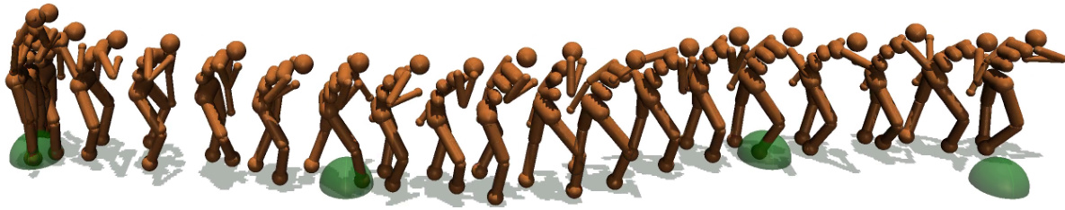
Figure 1: A humanoid agent discovers diverse locomotion primitives without any reward using DADS. We show zero-shot generalization to downstream tasks by composing the learned primitives using model predictive control, enabling the agent to follow an online sequence of goals (green markers) without any additional training.

图 1: 人形智能体通过DADS无奖励机制自主发现多样化运动基元。我们展示了通过模型预测控制组合所学基元的零样本下游任务泛化能力，使智能体无需额外训练即可跟随在线目标序列 (绿色标记) 。

1 INTRODUCTION

1 引言

Deep reinforcement learning (RL) enables autonomous learning of diverse and complex tasks with rich sensory inputs, temporally extended goals, and challenging dynamics, such as discrete gameplaying domains (Mnih et al., 2013; Silver et al., 2016), and continuous control domains including locomotion (Schulman et al., 2015; Heess et al., 2017) and manipulation (Rajeswaran et al., 2017; Kalashnikov et al., 2018; Gu et al., 2017). Most of the deep RL approaches learn a Q-function or a policy that are directly optimized for the training task, which limits their generalization to new scenarios. In contrast, MBRL methods (Li & Todorov, 2004; Deisenroth & Rasmussen, 2011; Watter et al., 2015) can acquire dynamics models that may be utilized to perform unseen tasks at test time. While this capability has been demonstrated in some of the recent works (Levine et al., 2016; Nagabandi et al., 2018; Chua et al., 2018b; Kurutach et al., 2018; Ha & Schmid huber,

深度强化学习 (RL) 能够通过丰富的感官输入、时间延伸目标和具有挑战性的动态环境，自主完成多样且复杂的任务，例如离散游戏领域 (Mnih et al., 2013; Silver et al., 2016) 以及包括运动控制 (Schulman et al., 2015; Heess et al., 2017) 和操作任务 (Rajeswaran et al., 2017; Kalashnikov et al., 2018; Gu et al., 2017) 在内的连续控制领域。大多数深度强化学习方法通过学习直接针对训练任务优化的 Q 函数或策略，这限制了它们对新场景的泛化能力。相比之下，基于模型的强化学习 (MBRL) 方法 (Li & Todorov, 2004; Deisenroth & Rasmussen, 2011; Watter et al., 2015) 能够获取动态模型，这些模型可用于在测试时执行未见过的任务。尽管这种能力已在一些近期工作中得到验证 (Levine et al., 2016; Nagabandi et al., 2018; Chua et al., 2018b; Kurutach et al., 2018; Ha & Schmidhuber,

2018), learning an accurate global model that works for all state-action pairs can be exceedingly challenging, especially for high-dimensional system with complex and discontinuous dynamics. The problem is further exacerbated as the learned global model has limited generalization outside of the state distribution it was trained on and exploring the whole state space is generally infeasible. Can we retain the flexibility of model-based RL, while using model-free RL to acquire proficient low-level behaviors under complex dynamics?

2018年)，学习一个适用于所有状态-动作对的精确全局模型可能极具挑战性，尤其是对于具有复杂且不连续动态的高维系统。当所学全局模型在其训练状态分布之外的泛化能力有限，且探索整个状态空间通常不可行时，问题会进一步加剧。我们能否在保留基于模型的强化学习灵活性的同时，利用无模型强化学习在复杂动态下获取熟练的低层行为？

While learning a global dynamics model that captures all the different behaviors for the entire statespace can be extremely challenging, learning a model for a specific behavior that acts only in a small part of the state-space can be much easier. For example, consider learning a model for dynamics of all gaits of a quadruped versus a model which only works for a specific gait. If we can learn many such behaviors and their corresponding dynamics, we can leverage model-predictive control to plan in the behavior space, as opposed to planning in the action space. The question then becomes: how do we acquire such behaviors, considering that behaviors could be random and unpredictable? To this end, we propose Dynamics-Aware Discovery of Skills (DADS), an unsupervised RL framework for learning low-level skills using model-free RL with the explicit aim of making model-based control easy. Skills obtained using DADS are directly optimized for predictability, providing a better representation on top of which predictive models can be learned. Crucially, the skills do not require any supervision to learn, and are acquired entirely through autonomous exploration. This means that the repertoire of skills and their predictive model are learned before the agent has been tasked with any goal or reward function. When a task is provided at test-time, the agent utilizes the previously learned skills and model to immediately perform the task without any further training.

虽然学习一个能捕捉整个状态空间所有不同行为的全局动态模型极具挑战性，但针对只在状态空间小范围内运作的特定行为学习模型则简单得多。例如，比较学习四足动物所有步态动态的模型与仅适用于特定步态的模型。如果我们能学习多种此类行为及其对应动态，就能利用模型预测控制在行为空间进行规划，而非动作空间规划。随之而来的问题是：考虑到行为可能随机且不可预测，我们如何获取这些行为？为此，我们提出动态感知技能发现(DADS)——一个通过无模型强化学习来获取底层技能的无监督强化学习框架，其明确目标是简化基于模型的控制。通过DADS获得的技能直接针对可预测性进行优化，为学习预测模型提供了更好的表征基础。关键在于，这些技能的学习无需任何监督，完全通过自主探索获得。这意味着技能库及其预测模型是在智能体被赋予任何目标或奖励函数之前就已习得的。当测试阶段提供任务时，智能体可立即调用预先学习的技能和模型来执行任务，无需额外训练。

The key contribution of our work is an unsupervised reinforcement learning algorithm, DADS, grounded in mutual-information-based exploration. We demonstrate that our objective can embed learned primitives in continuous spaces, which allows us to learn a large, diverse set of skills. Crucially, our algorithm also learns to model the dynamics of the skills, which enables the use of model-based planning algorithms for downstream tasks. We adapt the conventional model predictive control algorithms to plan in the space of primitives, and demonstrate that we can compose the learned primitives to solve downstream tasks without any additional training.

我们工作的核心贡献是一种基于互信息探索的无监督强化学习算法DADS。研究表明，该目标函数能够在连续空间中嵌入习得的基元技能，从而学习到大量多样化的技能组合。关键创新在于，该算法还能同步学习技能动态模型，这使得基于模型的规划算法能够直接应用于下游任务。我们改进了传统模型预测控制算法，使其能够在基元技能空间中进行规划，并验证了无需额外训练即可组合已学习技能来解决下游任务的能力。

2 PRELIMINARIES

2 预备知识

Mutual information can been used as an objective to encourage exploration in reinforcement learning (Houthooft et al., 2016; Mohamed & Rezende, 2015). According to its definition, $\mathcal{I}(X;Y)\stackrel{}{=}$ ${\mathcal{H}}(X)-{\mathcal{H}}(X\mid Y)$ , maximizing mutual information $\mathcal{T}$ with respect to $Y$ amounts to maximizing the entropy $\mathcal{H}$ of $X$ while minimizing the conditional entropy ${\mathcal{H}}(X\mid Y)$ . In the context of RL, $X$ is usually a function of the state and $Y$ a function of actions. Maximizing this objective encourages the state entropy to be high, making the underlying policy to be exploratory. Recently, multiple works (Eysenbach et al., 2018; Gregor et al., 2016; Achiam et al., 2018) apply this idea to learn diverse skills which maximally cover the state space.

互信息可作为强化学习中鼓励探索的目标函数 (Houthooft et al., 2016; Mohamed & Rezende, 2015)。根据其定义 $\mathcal{I}(X;Y)\stackrel{}{=}$ ${\mathcal{H}}(X)-{\mathcal{H}}(X\mid Y)$，最大化关于 $Y$ 的互信息 $\mathcal{T}$ 等价于最大化 $X$ 的熵 $\mathcal{H}$ 同时最小化条件熵 ${\mathcal{H}}(X\mid Y)$。在强化学习背景下，$X$ 通常是状态的函数，$Y$ 是动作的函数。最大化该目标函数会促使状态熵保持较高水平，从而使底层策略具有探索性。近期多项研究 (Eysenbach et al., 2018; Gregor et al., 2016; Achiam et al., 2018) 应用这一思想来学习能最大程度覆盖状态空间的多样化技能。

To leverage planning-based control, MBRL estimates the true dynamics of the environment by learning a model $\hat{p}(s^{\prime}\mid\bar{s},a)$ . This allows it to predict a trajectory of states $\hat{\tau}_ {H}=\left(s_{t},\hat{s}_ {t+1},,\dots\hat{s}_{t+H}\right)$ resulting from a sequence of actions without any additional interaction with the environment. While model-based RL methods have been demonstrated to be sample efficient compared to their modelfree counterparts, learning an effective model for the whole state-space is challenging. An openproblem in model-based RL is to incorporate temporal abstraction in model-based control, to enable high-level planning and move-away from planning at the granular level of actions.

为利用基于规划的控制，MBRL通过学习模型$\hat{p}(s^{\prime}\mid\bar{s},a)$来估计环境的真实动态。这使得它能够预测由一系列动作产生的状态轨迹$\hat{\tau}_ {H}=\left(s_{t},\hat{s}_ {t+1},,\dots\hat{s}_{t+H}\right)$，而无需与环境进行额外交互。尽管基于模型的强化学习方法已被证明比无模型方法更具样本效率，但为整个状态空间学习有效模型具有挑战性。基于模型强化学习中的一个开放问题是在基于模型的控制中融入时间抽象，以实现高层级规划并摆脱动作粒度的规划。

These seemingly unrelated ideas can be combined into a single optimization scheme, where we first discover skills (and their models) without any extrinsic reward and then compose these skills to optimize for the task defined at test time using model-based planning. At train time, we assume a Markov Decision Process (MDP) $\mathcal{M}_ {1}\equiv(\mathcal{S},\mathcal{A},p)$ . The state space $s$ and action space $\mathcal{A}$ are assumed to be continuous, and the $\mathcal{A}$ bounded. We assume the transition dynamics $p$ to be stochastic, such that $p:S\times{\mathcal{A}}\times{\mathcal{S}}\mapsto[0,\infty)$ . We learn a skill-conditioned policy $\pi(a\mid s,z)$ , where the skills $z$ belongs to the space $\mathcal{Z}$ , detailed in Section 3. We assume that the skills are sampled from a prior $p(z)$ over $\mathcal{Z}$ . We simultaneously learn a skill-conditioned transition function $q(s^{\prime}\mid s,z)$ , coined as skill-dynamics, which predicts the transition to the next state $s^{\prime}$ from the current state $s$ for the skill $z$ under the given dynamics $p$ . At test time, we assume an MDP $\mathcal{M}_ {2}\equiv(\mathcal{S},\mathcal{A},p,r)$ , where $S,{\cal A},p$ match those defined in $\mathcal{M}_ {1}$ , and the reward function $r:S\times A\mapsto(-\infty,\infty)$ . We plan in $\mathcal{Z}$ using $q(s^{\prime}\mid s,z)$ to compose the learned skills $z$ for optimizing $r$ in $\mathcal{M}_{2}$ , which we detail in Section 4.

这些看似无关的概念可以整合为单一的优化方案：首先在无外部奖励的情况下发现技能（及其模型），然后利用基于模型的规划在测试时将这些技能组合起来优化任务。训练时，我们假设一个马尔可夫决策过程 (MDP) $\mathcal{M}_ {1}\equiv(\mathcal{S},\mathcal{A},p)$。状态空间 $s$ 和动作空间 $\mathcal{A}$ 为连续空间，且 $\mathcal{A}$ 有界。假设转移动态 $p$ 是随机的，即 $p:S\times{\mathcal{A}}\times{\mathcal{S}}\mapsto[0,\infty)$。我们学习一个技能条件策略 $\pi(a\mid s,z)$，其中技能 $z$ 属于空间 $\mathcal{Z}$（详见第3节）。假设技能从 $\mathcal{Z}$ 上的先验分布 $p(z)$ 中采样得到。同时学习一个技能条件转移函数 $q(s^{\prime}\mid s,z)$（称为技能动态），用于在给定动态 $p$ 下预测技能 $z$ 从当前状态 $s$ 到下一状态 $s^{\prime}$ 的转移。测试时，假设存在 MDP $\mathcal{M}_ {2}\equiv(\mathcal{S},\mathcal{A},p,r)$，其中 $S,{\cal A},p$ 与 $\mathcal{M}_ {1}$ 定义一致，奖励函数为 $r:S\times A\mapsto(-\infty,\infty)$。我们在 $\mathcal{Z}$ 空间利用 $q(s^{\prime}\mid s,z)$ 进行规划，组合已学习技能 $z$ 以优化 $\mathcal{M}_{2}$ 中的 $r$（详见第4节）。

3 DYNAMICS-AWARE DISCOVERY OF SKILLS (DADS)

3 动态感知技能发现 (DADS)

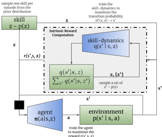
Figure 2: The agent $\pi$ interacts with the environment to produce a transition $s\rightarrow s^{\prime}$ . Intrinsic reward is computed by computing the transition probability under $q$ for the current skill $z$ , compared to random samples from the prior $p(\bar{z})$ . The agent maximizes the intrinsic reward computed for a batch of episodes, while $q$ maximizes the log-probability of the actual transitions of $(s,z)\to s^{\prime}$ .

图 2: 智能体 $\pi$ 与环境交互产生状态转移 $s\rightarrow s^{\prime}$。内在奖励通过计算当前技能 $z$ 在 $q$ 下的转移概率，并与先验分布 $p(\bar{z})$ 的随机样本进行比较得出。智能体最大化由一批回合计算得到的内在奖励，同时 $q$ 最大化实际状态转移 $(s,z)\to s^{\prime}$ 的对数概率。

We use the information theoretic paradigm of mutual information to obtain our unsupervised skill discovery algorithm. In particular, we propose to maximize the mutual information between the next state $s^{\prime}$ and current skill $z$ conditioned on the current state $s$ .

我们采用互信息的信息论范式来开发无监督技能发现算法。具体而言，我们提出最大化下一状态$s^{\prime}$与当前技能$z$在给定当前状态$s$条件下的互信息。

$$
\begin{array}{r}{\mathbb{Z}(s^{\prime};z\mid s)=\mathcal{H}(z\mid s)-\mathcal{H}(z\mid s^{\prime},s)}\ {=\mathcal{H}(s^{\prime}\mid s)-\mathcal{H}(s^{\prime}\mid s,z)}\end{array}
$$

Mutual information in Equation 1 quantifies how much can be known about $s^{\prime}$ given $z$ and $s$ , or symmetrically, $z$ given the transition from $s\rightarrow s^{\prime}$ . From Equation 2, maximizing this objective corresponds to maximizing the diversity of transitions produced in the environment, that is denoted by the entropy $\mathcal{H}(s^{\prime}\mid s)$ , while making $z$ informative about the next state $s^{\prime}$ by minimizing the entropy $\mathcal{H}(s^{\prime}\mid s,z)$ . Intuitively, skills $z$ can be interpreted as abstracted action sequences which are identifiable by the transitions generated in the environment (and not just by the current state). Thus, optimizing this mutual information can be understood as encoding a diverse set of skills in the latent space $\mathcal{Z}$ , while making the transitions for a given $z\in{\mathcal{Z}}$ predictable. We use the entropydecomposition in Equation 2 to connect this objective with model-based control.

式1中的互信息量化了在给定$z$和$s$时能获知多少关于$s^{\prime}$的信息（对称地，也可量化在状态转移$s\rightarrow s^{\prime}$时能获知多少关于$z$的信息）。根据式2，最大化该目标函数等价于最大化环境中状态转移的多样性（即熵$\mathcal{H}(s^{\prime}\mid s)$），同时通过最小化熵$\mathcal{H}(s^{\prime}\mid s,z)$使$z$能有效预测下一状态$s^{\prime}$。直观上，技能$z$可解释为被环境生成的状态转移（而非仅当前状态）所标识的抽象动作序列。因此，优化该互信息可理解为在潜在空间$\mathcal{Z}$中编码多样化的技能集，同时确保给定$z\in{\mathcal{Z}}$时的状态转移具有可预测性。我们利用式2的熵分解将此目标函数与基于模型的控制建立关联。

We want to optimize the our skill-conditioned controller $\pi(a\mid s,z)$ such that the latent space $z\sim p(z)$ is maximally informative about the transitions $s\to s^{\prime}$ . Using the definition of conditional mutual information, we can rewrite Equation 2 as:

我们想要优化技能条件控制器 $\pi(a\mid s,z)$，使得潜在空间 $z\sim p(z)$ 能最大化地反映状态转移 $s\to s^{\prime}$ 的信息。利用条件互信息的定义，我们可以将公式2重写为：

$$
\mathcal{Z}(s^{\prime};z\mid s)=\int p(z,s,s^{\prime})\log\frac{p(s^{\prime}\mid s,z)}{p(s^{\prime}\mid s)}d s^{\prime}d s d z
$$

We assume the following generative model: $p(z,s,s^{\prime})=p(z)p(s\mid z)p(s^{\prime}\mid s,z)$ , where $p(z)$ is user specified prior over $\mathcal{Z}$ , $p(s|z)$ denotes the stationary state-distribution induced by $\pi(a\mid s,z)$ for a skill $z$ and $p(s^{\prime}\mid s,z)$ denotes the transition distribution under skill $z$ . Note, $p(s^{\prime}\mid s,z)=$ $\begin{array}{r}{\int p(s^{\prime}\mid s,a)\pi(a\mid\dot{s},z)d a}\end{array}$ is intractable to compute because the underlying dynamics are unknown. However, we can variation ally lower bound the objective as follows:

我们假设以下生成模型：$p(z,s,s^{\prime})=p(z)p(s\mid z)p(s^{\prime}\mid s,z)$，其中$p(z)$是用户指定的$\mathcal{Z}$上的先验分布，$p(s|z)$表示由技能$z$的策略$\pi(a\mid s,z)$诱导的稳态分布，$p(s^{\prime}\mid s,z)$表示技能$z$下的转移分布。注意，$p(s^{\prime}\mid s,z)=$$\begin{array}{r}{\int p(s^{\prime}\mid s,a)\pi(a\mid\dot{s},z)d a}\end{array}$由于底层动态未知而难以计算。然而，我们可以通过以下方式变分下界目标：

$$
\begin{array}{r l}&{\mathbb{Z}(s^{\prime};z\mid s)=\mathbb{E}_ {z,s,s^{\prime}\sim p}\Big[\log\frac{p(s^{\prime}\mid s,z)}{p(s^{\prime}\mid s)}\Big]}\ &{\qquad=\mathbb{E}_ {z,s,s^{\prime}\sim p}\Big[\log\frac{q_{\phi}(s^{\prime}\mid s,z)}{p(s^{\prime}\mid s)}\Big]+\mathbb{E}_ {s,z\sim p}\Big[\mathcal{D}_ {K L}(p(s^{\prime}\mid s,z)\mid\mid q_{\phi}(s^{\prime}\mid s,z))\Big]}\ &{\qquad\geq\mathbb{E}_ {z,s,s^{\prime}\sim p}\Big[\log\frac{q_{\phi}(s^{\prime}\mid s,z)}{p(s^{\prime}\mid s)}\Big]}\end{array}
$$

where we have used the non-negativity of KL-divergence, that is $\mathcal{D}_ {K L}\geq0$ . Note, skill-dynamics $q_{\phi}$ represents the variation al approximation for the transition function $p(s^{\prime}\mid s,z)$ , which enables model-based control as described in Section 4. Equation 4 suggests an alternating optimization between $q_{\phi}$ and $\pi$ , summarized in Algorithm 1. In every iteration:

其中我们利用了KL散度的非负性，即 $\mathcal{D}_ {K L}\geq0$ 。注意，技能动态 $q_{\phi}$ 表示对转移函数 $p(s^{\prime}\mid s,z)$ 的变分近似，如第4节所述，这支持基于模型的控制。公式4提出了 $q_{\phi}$ 和 $\pi$ 之间的交替优化，如算法1所总结。在每次迭代中：

(Tighten variation al lower bound) We minimize $D_{K L}(p(s^{\prime}\mid s,z)\mid\mid q_{\phi}(s^{\prime}\mid s,z))$ with respect to the parameters $\phi$ on $z,s\sim p$ to tighten the lower bound. For general function ap proxima tors like neural networks, we can write the gradient for $\phi$ as follows:

(收紧变分下界) 我们最小化 $D_{K L}(p(s^{\prime}\mid s,z)\mid\mid q_{\phi}(s^{\prime}\mid s,z))$ 关于参数 $\phi$ 在 $z,s\sim p$ 上的取值，以收紧下界。对于神经网络等通用函数逼近器，可将 $\phi$ 的梯度表示为:

$$
\begin{array}{r}{\nabla_{\phi}\mathbb{E}_ {s,z}[\mathcal{D}_ {K L}(p(s^{\prime}\mid s,z)\mid\mid q_{\phi}(s^{\prime}\mid s,z))]=\nabla_{\phi}\mathbb{E}_ {z,s,s^{\prime}}\Big[\log\frac{p(s^{\prime}\mid s,z)}{q_{\phi}(s^{\prime}\mid s,z)}\Big]}\ {=-\mathbb{E}_ {z,s,s^{\prime}}\Big[\nabla_{\phi}\log q_{\phi}(s^{\prime}\mid s,z)\Big]}\end{array}
$$

which corresponds to maximizing the likelihood of the samples from $p$ under $q_{\phi}$ .

这相当于在 $q_{\phi}$ 下最大化来自 $p$ 的样本的似然。

(Maximize approximate lower bound) After fitting $q_{\phi}$ , we can optimize $\pi$ to maximize $\mathbb{E}_ {z,s,s^{\prime}}[\log q_{\phi}(s^{\prime}\mid s,z)-\log p(s^{\prime}\mid s)]$ . Note, this is a reinforcement-learning style optimization with a reward function $\log q_{\phi}(s^{\prime}\mid s,z)-\log p(s^{\prime}\mid s)$ . However, $\log p(s^{\prime}\mid s)$ is intractable to compute, so we approximate the reward function for $\pi$ :

（最大化近似下界）拟合 $q_{\phi}$ 后，我们可以优化 $\pi$ 以最大化 $\mathbb{E}_ {z,s,s^{\prime}}[\log q_{\phi}(s^{\prime}\mid s,z)-\log p(s^{\prime}\mid s)]$。注意，这是一个强化学习风格的优化，其奖励函数为 $\log q_{\phi}(s^{\prime}\mid s,z)-\log p(s^{\prime}\mid s)$。然而，$\log p(s^{\prime}\mid s)$ 难以计算，因此我们为 $\pi$ 近似奖励函数：

$$
r_{z}(s,a,s^{\prime})=\log\frac{q_{\phi}(s^{\prime}\mid s,z)}{\sum_{i=1}^{L}q_{\phi}(s^{\prime}\mid s,z_{i})}+\log L,\quad z_{i}\sim p(z).
$$

The approximation is motivated as follows: $\begin{array}{r}{p(s^{\prime}\mid s)=\int p(s^{\prime}\mid s,z)p(z\mid s)d z\approx\int q_{\phi}(s^{\prime}\mid}\end{array}$ $\begin{array}{r}{s,z)p(z)d z\approx\frac{1}{L}\sum_{i=1}^{L}q_{\phi}(s^{\prime}\mid s,z_{i})}\end{array}$ for $z_{i}\sim p(z)$ , where $L$ denotes the number o mples from the prior. We are using the marginal of variation al approximation $p(z)$ imate the marginal distribution of transitions. We discuss this approximation in Appendix C. Note, the final reward function $r_{z}$ encourages the policy $\pi$ to produce transitions that are (a) predictable under $q_{\phi}$ (predictability) and (b) different from the transitions produced under $z_{i}\sim p(z)$ (diversity).

该近似方法的动机如下：$\begin{array}{r}{p(s^{\prime}\mid s)=\int p(s^{\prime}\mid s,z)p(z\mid s)d z\approx\int q_{\phi}(s^{\prime}\mid}\end{array}$ $\begin{array}{r}{s,z)p(z)d z\approx\frac{1}{L}\sum_{i=1}^{L}q_{\phi}(s^{\prime}\mid s,z_{i})}\end{array}$ 其中 $z_{i}\sim p(z)$，$L$ 表示从先验分布中采样的数量。我们使用变分近似的边缘分布 $p(z)$ 来近似转移的边缘分布。该近似方法的讨论详见附录C。需注意，最终奖励函数 $r_{z}$ 会激励策略 $\pi$ 产生符合以下特性的状态转移：(a) 在 $q_{\phi}$ 下可预测（可预测性），(b) 与 $z_{i}\sim p(z)$ 下产生的转移不同（多样性）。

To generate samples from $p(z,s,s^{\prime})$ , we use the rollouts from the current policy $\pi$ for multiple samples $z\sim p(z)$ in an episodic setting for a fixed horizon $T$ . We also introduce entropy regularization for $\pi(a\mid s,z)$ , which encourages the policy to discover action-sequences with similar state-transitions and to be clustered under the same skill $z$ , making the policy robust besides encouraging exploration (Haarnoja et al., 2018a). The use of entropy regular iz ation can be justified from an information bottleneck perspective as discussed for Information Maximization algorithm in (Mohamed & Rezende, 2015). This is even more extensively discussed from the graphical model perspective in Appendix B, which connects unsupervised skill discovery and information bottleneck literature, while also revealing the temporal nature of skills $z$ . Details corresponding to implementation and hyper parameters are discussed in Appendix A.

为了从 $p(z,s,s^{\prime})$ 生成样本，我们在固定时间范围 $T$ 的情景设置中，使用当前策略 $\pi$ 的多次采样 $z\sim p(z)$ 进行滚动计算。我们还对 $\pi(a\mid s,z)$ 引入了熵正则化 (entropy regularization) ，这鼓励策略发现具有相似状态转移的动作序列，并将其聚类到同一技能 $z$ 下，从而在促进探索的同时增强策略的鲁棒性 (Haarnoja et al., 2018a) 。从信息瓶颈 (information bottleneck) 的角度来看，熵正则化的使用是合理的，如 (Mohamed & Rezende, 2015) 中关于信息最大化算法 (Information Maximization algorithm) 的讨论所示。附录 B 从图模型的角度对此进行了更广泛的讨论，将无监督技能发现与信息瓶颈文献联系起来，同时揭示了技能 $z$ 的时间特性。实现细节和超参数相关内容详见附录 A。

4 PLANNING USING SKILL DYNAMICS

4 基于技能动态的规划

Given the learned skills $\pi(a\mid s,z)$ and their respective skill-transition dynamics $q_{\phi}(s^{\prime}\mid s,z)$ , we can perform model-based planning in the latent space $\mathcal{Z}$ to optimize for a reward $r$ that is given to the agent at test time. Note, that this essentially allows us to perform zero-shot planning given the unsupervised pre-training procedure described in Section 3.

给定学习到的技能 $\pi(a\mid s,z)$ 及其各自的技能转移动态 $q_{\phi}(s^{\prime}\mid s,z)$，我们可以在潜在空间 $\mathcal{Z}$ 中进行基于模型的规划，以优化测试时赋予智能体的奖励 $r$。值得注意的是，这本质上使我们能够基于第3节描述的无监督预训练过程进行零样本 (Zero-shot) 规划。

In order to perform planning, we employ the model-predictive-control (MPC) paradigm Garcia et al. (1989), which in a standard setting generates a set of action plans $P_{k}=(a_{k,1},...a_{k,H})\sim P$ for a planning horizon $H$ . The MPC plans can be generated due to the fact that the planner is able to simulate the trajectory $\hat{\tau}_ {k}=\left(s_{k,1},a_{k,1}...s_{k,H+1}\right)$ assuming access to the transition dynamics ${\hat{p}}(s^{\prime}\mid s,a)$ . In addition, each plan computes the reward $r(\hat{\tau}_ {k})$ for its trajectory according to the reward function $r$ that is provided for the test-time task. Following the MPC principle, the planner selects the best plan according to the reward function $r$ and executes its first action $a_{1}$ . The planning algorithm repeats this procedure for the next state iterative ly until it achieves its goal.

为了进行规划，我们采用了模型预测控制 (MPC) 范式 [Garcia et al. (1989)]，在标准设置下，它会为规划周期 $H$ 生成一组动作计划 $P_{k}=(a_{k,1},...a_{k,H})\sim P$。MPC 计划之所以能够生成，是因为规划器能够模拟轨迹 $\hat{\tau}_ {k}=\left(s_{k,1},a_{k,1}...s_{k,H+1}\right)$，前提是可以访问转移动态 ${\hat{p}}(s^{\prime}\mid s,a)$。此外，每个计划会根据为测试时任务提供的奖励函数 $r$ 计算其轨迹的奖励 $r(\hat{\tau}_ {k})$。根据 MPC 原则，规划器会按照奖励函数 $r$ 选择最佳计划并执行其第一个动作 $a_{1}$。规划算法会在下一个状态重复此过程，直到达成目标。

We use a similar strategy to design an MPC planner to exploit previously-learned skill-transition dynamics $q_{\phi}(s^{\prime}\mid s,z)$ . Note that unlike conventional model-based RL, we generate a plan $P_{k}={}$ $\big(z_{k,1},\dots:z_{k,H_{P}}\big)$ in the latent space $\mathcal{Z}$ as opposed to the action space $\mathcal{A}$ that would be used by a standard planner. Since the primitives are temporally meaningful, it is beneficial to hold a primitive for a horizon $H_{Z}>1$ , unlike actions which are usually held for a single step. Thus, effectively, the planning horizon for our latent space planner is $H=H_{P}\times H_{Z}$ , enabling longer-horizon planning using fewer primitives. Similar to the standard MPC setting, the latent space planner simulates the trajectory $\hat{\tau}_ {k}=\left(s_{k,1},z_{k,1},a_{k,1},s_{k,2},z_{k,2},a_{k,2},\dots s_{k,H+1}\right)$ and computes the reward $r(\hat{\tau}_ {k})$ . After a small number of trajectory samples, the planner selects the first latent action $z_{1}$ of the best plan, executes it for $H_{Z}$ steps in the environment, and the repeats the process until goal completion.

我们采用类似策略设计了一个MPC规划器，以利用先前学习的技能转移动态$q_{\phi}(s^{\prime}\mid s,z)$。需要注意的是，与传统基于模型的强化学习不同，我们在潜在空间$\mathcal{Z}$中生成计划$P_{k}={}$$\big(z_{k,1},\dots:z_{k,H_{P}}\big)$，而非标准规划器使用的动作空间$\mathcal{A}$。由于基元具有时序意义，保持一个基元持续$H_{Z}>1$步长比单步执行动作更具优势。因此，潜在空间规划器的有效规划范围为$H=H_{P}\times H_{Z}$，使得用更少基元实现更长跨度规划成为可能。与标准MPC设置类似，该规划器模拟轨迹$\hat{\tau}_ {k}=\left(s_{k,1},z_{k,1},a_{k,1},s_{k,2},z_{k,2},a_{k,2},\dots s_{k,H+1}\right)$并计算奖励$r(\hat{\tau}_ {k})$。经过少量轨迹采样后，规划器选择最优计划的第一个潜在动作$z_{1}$，在环境中执行$H_{Z}$步，然后重复该过程直至达成目标。

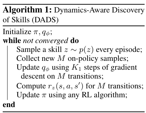
Figure 3: At test time, the planner executes simulates the transitions in environment using skill-dynamics $q$ , and updates the distribution of plans according to the computed reward on the simulated trajectories. After a few updates to the plan, the first primitive is executed in the environment using the learned agent $\pi$ .

图 3: 在测试阶段，规划器使用技能动力学 $q$ 模拟环境中的状态转移，并根据模拟轨迹上的计算奖励更新计划分布。经过几次计划更新后，第一个基元动作通过已学习的智能体 $\pi$ 在环境中执行。

The latent planner $P$ maintains a distribution of latent plans, each of length $H_{P}$ . Each element in the sequence represents the distribution of the primitive to be executed at that time step. For continuous spaces, each element of the sequence can be modelled using a normal distribution, $\mathcal{N}(\mu_{1},\Sigma),\dots\mathcal{N}(\mu_{H_{P}},\Sigma)$ . We refine the planning distributions for $R$ steps, using $K$ samples of latent plans $P_{k}$ , and compute the $r_{k}$ for the simulated trajectory $\hat{\tau}_{k}$ . The update for the parameters follows that in Model Predictive Path Integral (MPPI) controller Williams et al. (2016):

潜在规划器 $P$ 维持着一组长度为 $H_{P}$ 的潜在计划分布。序列中的每个元素代表该时间步要执行的基本动作分布。对于连续空间，序列的每个元素可以用正态分布建模，即 $\mathcal{N}(\mu_{1},\Sigma),\dots\mathcal{N}(\mu_{H_{P}},\Sigma)$。我们通过采样 $K$ 个潜在计划 $P_{k}$，对规划分布进行 $R$ 步优化，并计算模拟轨迹 $\hat{\tau}_ {k}$ 的奖励 $r_{k}$。参数更新遵循模型预测路径积分 (MPPI) 控制器的规则 (Williams et al., 2016)：

$$
\mu_{i}=\sum_{k=1}^{K}\frac{\exp(\gamma r_{k})}{\sum_{p=1}^{K}\exp(\gamma r_{p})}z_{k,i}\quad\forall i=1,\dots{\cal H}_{P}
$$

While we keep the covariance matrix of the distributions fixed, it is possible to update that as well as shown in Williams et al. (2016). We show an overview of the planning algorithm in Figure 3, and provide more implementation details in Appendix A.

虽然我们保持分布的协方差矩阵固定，但也可以按照 Williams 等人 (2016) 所示的方法进行更新。我们在图 3 中展示了规划算法的概览，并在附录 A 中提供了更多实现细节。

5 相关工作

Central to our method is the concept of skill discovery via mutual information maximization. This principle, proposed in prior work that utilized purely model-free unsupervised RL methods (Daniel et al., 2012; Florensa et al., 2017; Eysenbach et al., 2018; Gregor et al., 2016; Warde-Farley et al., 2018; Thomas et al., 2018), aims to learn diverse skills via a disc rim inability objective: a good set of skills is one where it is easy to distinguish the skills from each other, which means they perform distinct tasks and cover the space of possible behaviors. Building on this prior work, we distinguish our skills based on how they modify the original uncontrolled dynamics of the system. This simultaneously encourages the skills to be both diverse and predictable. We also demonstrate that constraining the skills to be predictable makes them more amenable for hierarchical composition and thus, more useful on downstream tasks.

我们方法的核心是通过互信息最大化实现技能发现。这一原则源自先前采用纯无模型无监督强化学习方法的研究 (Daniel et al., 2012; Florensa et al., 2017; Eysenbach et al., 2018; Gregor et al., 2016; Warde-Farley et al., 2018; Thomas et al., 2018) ，其目标是通过可判别性目标学习多样化技能：优质的技能组合应易于相互区分，这意味着它们执行不同任务并覆盖可能的行为空间。基于这些研究基础，我们根据技能如何改变系统原始非受控动态来区分技能。这种方法同时促进技能的多样性和可预测性。我们还证明，约束技能的可预测性使其更适用于层次化组合，从而在下游任务中更具实用性。

Another line of work that is conceptually close to our method copes with intrinsic motivation (Oudeyer & Kaplan, 2009; Oudeyer et al., 2007; Schmid huber, 2010) which is used to drive the agent’s exploration. Examples of such works include empowerment Klyubin et al. (2005); Mohamed & Rezende (2015), count-based exploration Bellemare et al. (2016); Oh et al. (2015); Tang et al. (2017); Fu et al. (2017), information gain about agent’s dynamics Stadie et al. (2015) and forward-inverse dynamics models Pathak et al. (2017). While our method uses an informationtheoretic objective that is similar to these approaches, it is used to learn a variety of skills that can be directly used for model-based planning, which is in contrast to learning a better exploration policy for a single skill.

另一项在概念上与我们方法相近的工作涉及内在动机 (Oudeyer & Kaplan, 2009; Oudeyer et al., 2007; Schmidhuber, 2010)，用于驱动智能体的探索。这类工作的例子包括赋能 (Klyubin et al., 2005; Mohamed & Rezende, 2015)、基于计数的探索 (Bellemare et al., 2016; Oh et al., 2015; Tang et al., 2017; Fu et al., 2017)、关于智能体动态的信息增益 (Stadie et al., 2015) 以及前向-逆向动态模型 (Pathak et al., 2017)。虽然我们的方法使用了与这些方法类似的信息论目标，但它用于学习多种可直接用于基于模型规划的技能，这与为单一技能学习更好的探索策略形成对比。

The skills discovered using our approach can also provide extended actions and temporal abstraction, which enable more efficient exploration for the agent to solve various tasks, reminiscent of hierarchical RL (HRL) approaches. This ranges from the classic option-critic architecture (Sutton et al., 1999; Stolle & Precup, 2002; Perkins et al., 1999) to some of the more recent work (Bacon et al., 2017; Vezhnevets et al., 2017; Nachum et al., 2018; Hausman et al., 2018). However, in contrast to end-to-end HRL approaches (Heess et al., 2016; Peng et al., 2017), we can leverage a stable, two-phase learning setup. The primitives learned through our method provide action and temporal abstraction, while planning with skill-dynamics enables hierarchical composition of these primitives, bypassing many problems of end-to-end HRL.

通过我们的方法发现的技能还能提供扩展动作和时间抽象能力，使得智能体在解决各类任务时能进行更高效的探索，这让人联想到分层强化学习 (HRL) 方法。这类方法涵盖从经典选项-评论家架构 (Sutton et al., 1999; Stolle & Precup, 2002; Perkins et al., 1999) 到近年研究 (Bacon et al., 2017; Vezhnevets et al., 2017; Nachum et al., 2018; Hausman et al., 2018) 。但与端到端HRL方法 (Heess et al., 2016; Peng et al., 2017) 不同，我们采用了稳定的两阶段学习框架：通过本方法学习的基础技能提供动作与时间抽象能力，而基于技能动力学的规划则实现了这些基础技能的分层组合，从而规避了端到端HRL的诸多问题。

In the second phase of our approach, we use the learned skill-transition dynamics models to perform model-based planning - an idea that has been explored numerous times in the literature. Model-based reinforcement learning has been traditionally approached with methods that are well-suited for lowdata regimes such as Gaussian Processes (Rasmussen, 2003) showing significant data-efficiency gains over model-free approaches (Deisenroth et al., 2013; Kamthe & Deisenroth, 2017; Kocijan et al., 2004; Ko et al., 2007). More recently, due to the challenges of applying these methods to highdimensional state spaces, MBRL approaches employs Bayesian deep neural networks (Nagabandi et al., 2018; Chua et al., 2018b; Gal et al., 2016; Fu et al., 2016; Lenz et al., 2015) to learn dynamics models. In our approach, we take advantage of the deep dynamics models that are conditioned on the skill being executed, simplifying the modelling problem. In addition, the skills themselves are being learned with the objective of being predictable, further assists with the learning of the dynamics model. There also have been multiple approaches addressing the planning component of MBRL including linear controllers for local models (Levine et al., 2016; Kumar et al., 2016; Chebotar et al., 2017), uncertainty-aware (Chua et al., 2018b; Gal et al., 2016) or deterministic planners (Nagabandi et al., 2018) and stochastic optimization methods (Williams et al., 2016). The main contribution of our work lies in discovering model-based skill primitives that can be further combined by a standard model-based planner, therefore we take advantage of an existing planning approach - Model Predictive Path Integral (Williams et al., 2016) that can leverage our pre-trained setting.

在我们方法的第二阶段，利用学习到的技能转移动态模型进行基于模型的规划——这一思路在文献中已被多次探讨。传统上，基于模型的强化学习采用高斯过程 (Gaussian Processes) [Rasmussen, 2003] 等适用于低数据量场景的方法，相比无模型方法展现出显著的数据效率优势 [Deisenroth et al., 2013; Kamthe & Deisenroth, 2017; Kocijan et al., 2004; Ko et al., 2007]。近年来，针对高维状态空间的建模挑战，基于模型的强化学习方法开始采用贝叶斯深度神经网络 [Nagabandi et al., 2018; Chua et al., 2018b; Gal et al., 2016; Fu et al., 2016; Lenz et al., 2015] 来学习动态模型。我们的方法利用以执行技能为条件的深度动态模型，简化了建模问题。此外，技能本身以可预测性为目标进行学习，进一步辅助动态模型的学习。针对基于模型强化学习的规划环节，现有方法包括局部模型的线性控制器 [Levine et al., 2016; Kumar et al., 2016; Chebotar et al., 2017]、不确定性感知 [Chua et al., 2018b; Gal et al., 2016] 或确定性规划器 [Nagabandi et al., 2018] 以及随机优化方法 [Williams et al., 2016]。本工作的核心贡献在于发现可被标准基于模型规划器进一步组合的模型化技能基元，因此我们采用现有规划方法——模型预测路径积分 (Model Predictive Path Integral) [Williams et al., 2016]，该方法能有效利用我们的预训练设置。

6 EXPERIMENTS

6 实验

Through our experiments, we aim to demonstrate that: (a) DADS as a general purpose skill discovery algorithm can scale to high-dimensional problems; (b) discovered skills are amenable to hierarchical composition and; (c) not only is planning in the learned latent space feasible, but it is competitive to strong baselines. In Section 6.1, we provide visualization s and qualitative analysis of the skills learned using DADS. We demonstrate in Section 6.2 and Section 6.4 that optimizing the primitives for predictability renders skills more amenable to temporal composition that can be used for Hierarchical RL.We benchmark against state-of-the-art model-based RL baseline in Section 6.3, and against goal-conditioned RL in Section 6.5.

通过实验，我们旨在证明：(a) DADS作为一种通用技能发现算法能够扩展到高维问题；(b) 发现的技能适合分层组合；(c) 在学习的潜在空间中进行规划不仅可行，而且能与强基线方法竞争。在6.1节中，我们提供了使用DADS学习技能的可视化及定性分析。6.2节和6.4节证明，通过优化基元可预测性可使技能更适用于时序组合，从而用于分层强化学习。6.3节我们对比了最先进的基于模型的强化学习基线方法，6.5节则对比了目标条件强化学习方法。

6.1 QUALITATIVE ANALYSIS

6.1 定性分析

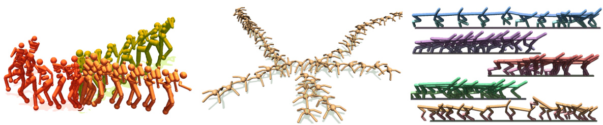
Figure 4: Skills learned on different MuJoCo environments in the OpenAI gym. DADS can discover diverse skills without any extrinsic rewards, even for problems with high-dimensional state and action spaces.

图 4: 在OpenAI gym的不同MuJoCo环境中学习到的技能。DADS无需任何外部奖励即可发现多样化技能，即便面对高维状态和动作空间的问题也是如此。

In this section, we provide a qualitative discussion of the unsupervised skills learned using DADS. We use the MuJoCo environments (Todorov et al., 2012) from the OpenAI gym as our test-bed (Brockman et al., 2016). We find that our proposed algorithm can learn diverse skills without any reward, even in problems with high-dimensional state and actuation, as illustrated in Figure 4. DADS can discover primitives for Half-Cheetah to run forward and backward with multiple different gaits, for Ant to navigate the environment using diverse locomotion primitives and for Humanoid to walk using stable locomotion primitives with diverse gaits and direction. The videos of the discovered primitives are available at: https://sites.google.com/view/dads-skill

在本节中，我们定性讨论使用DADS学习的无监督技能。我们以OpenAI gym中的MuJoCo环境 [Todorov et al., 2012] 作为测试平台 [Brockman et al., 2016] 。如图4所示，我们发现所提算法能在无奖励条件下学习多样化技能，即使在高维状态与执行机构的问题中。DADS能为Half-Cheetah发现前进/后退的多步态运动基元，为Ant发现多种移动基元以实现环境导航，并为人形机器人(Humanoid)发现具有多样步态和方向的稳定运动基元。技能发现视频详见: https://sites.google.com/view/dads-skill

Qualitatively, we find the skills discovered by DADS to be predictable and stable, in line with implicit constraints of the proposed objective. While the Half-Cheetah will learn to run in both backward and forward directions, DADS will d is in centi viz e skills which make Half-Cheetah flip owing to the reduced predictability on landing. Similarly, skills discovered for Ant rarely flip over, and tend to provide stable navigation primitives in the environment. This also in centi viz es the Humanoid, which is characteristically prone to collapsing and extremely unstable by design, to discover gaits which are stable for sustainable locomotion.

定性地看，我们发现DADS发现的技能具有可预测性和稳定性，符合所提出目标的隐含约束。虽然Half-Cheetah会学习向前和向后奔跑，但DADS会优先选择那些使Half-Cheetah翻转的技能，因为着陆时的可预测性降低。类似地，为Ant发现的技能很少会翻转，并倾向于在环境中提供稳定的导航原语。这也促使Humanoid（其设计特性容易倒塌且极不稳定）发现适合持续运动的稳定步态。

One of the significant advantages of the proposed objective is that it is compatible with continuous skill spaces, which has not been shown in prior work on skill discovery (Eysenbach et al., 2018). Not only does this allow us to embed a large and diverse set of skills into a compact latent space, but also the smoothness of the learned space allows us to interpolate between behaviors generated in the environment. We demonstrate this on the Ant environment (Figure 5), where we learn two-dimensional continuous skill space with a uniform prior over $(-1,1)$ in each dimension, and compare it to a discrete skill space with a uniform prior over 20 skills. Similar to Eysenbach et al. (2018), we restrict the observation space of the skill-dynamics $q$ to the cartesian coordinates $(x,y)$ . We hereby call this the $x$ -y prior, and discuss its role in Section 6.2.

所提目标函数的一大显著优势在于其兼容连续技能空间，这一特性在先前技能发现研究中尚未得到验证 (Eysenbach et al., 2018)。这不仅使我们能够将大量多样化技能嵌入紧凑的潜在空间，所学空间的平滑性还支持对环境生成行为进行插值。我们在Ant环境中对此进行了演示 (图5)：通过在每个维度上建立(-1,1)均匀先验的二维连续技能空间，并与20个离散技能的均匀先验空间进行对比。与Eysenbach等人(2018)类似，我们将技能动力学q的观测空间限制在笛卡尔坐标(x,y)内。此处称其为x-y先验，其作用将在6.2节讨论。

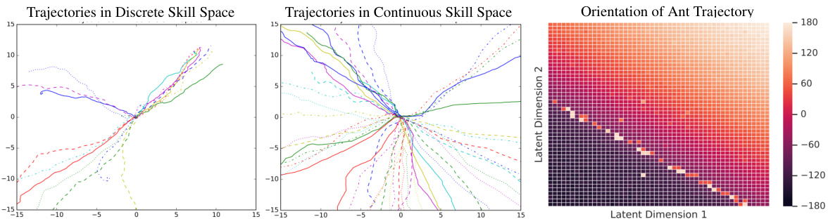
Figure 5: (Left, Centre) X-Y traces of Ant skills and (Right) Heatmap to visualize the learned continuous skill space. Traces demonstrate that the continuous space offers far greater diversity of skills, while the heatmap demonstrates that the learned space is smooth, as the orientation of the X-Y trace varies smoothly as a function of the skill.

图 5: (左, 中) 蚂蚁技能的X-Y轨迹和 (右) 可视化学习连续技能空间的热力图。轨迹表明连续空间提供了更大的技能多样性，而热力图显示学习空间是平滑的，因为X-Y轨迹的方向会随着技能参数平滑变化。

In Figure 5, we project the trajectories of the learned Ant skills from both discrete and continuous spaces onto the Cartesian plane. From the traces of the skills, it is clear that the continuous latent space can generate more diverse trajectories. We demonstrate in Section 6.3, that continuous primitives are more amenable to hierarchical composition and generally perform better on downstream tasks. More importantly, we observe that the learned skill space is semantically meaningful. The heatmap in Figure 5 shows the orientation of the trajectory (with respect to the $x$ -axis) as a function of the skill $z\in{\mathcal{Z}}$ , which varies smoothly as $z$ is varied, with explicit interpolations shown in Appendix D.

在图5中，我们将离散和连续空间中学到的Ant技能轨迹投影到笛卡尔平面上。从技能轨迹可以明显看出，连续潜在空间能生成更多样化的路径。第6.3节将证明，连续基元更适用于层次化组合，且通常在下游任务中表现更优。更重要的是，我们观察到所学技能空间具有语义意义。图5中的热力图展示了轨迹方向(相对于$x$轴)随技能$z\in{\mathcal{Z}}$变化的函数关系，当$z$变化时方向会平滑过渡，具体插值示例见附录D。

6.2 SKILL VARIANCE ANALYSIS

6.2 技能差异分析

In an unsupervised skill learning setup, it is important to optimize the primitives to be diverse. However, we argue that diversity is not sufficient for the learned primitives to be useful for downstream tasks. Primitives must exhibit low-variance behavior, which enables long-horizon composition of the learned skills in a hierarchical setup. We analyze the variance of the $x{-}y$ trajectories in the environment, where we also benchmark the variance of the primitives learned by DIAYN (Eysenbach et al., 2018). For DIAYN, we use the $x{-}y$ prior for the skill-disc rim in at or, which biases the discovered skills to diversify in the x-y space. This step was necessary for that baseline to obtain a competitive set of navigation skills. Figure 6 (Top-Left) demonstrates that DADS, which optimizes the primitives for predictability and diversity, yields significantly lower-variance primitives when compared to DIAYN, which only optimizes for diversity. This is starkly demonstrated in the plots of X-Y traces of skills learned in different setups. Skills learned by DADS show significant control over the trajectories generated in the environment, while skills from DIAYN exhibit high variance in the environment, which limits their utility for hierarchical control. This is further demonstrated quantitatively in Section 6.4.

在无监督技能学习设置中，优化基元以实现多样性至关重要。但我们认为，仅靠多样性不足以使所学基元对下游任务有用。基元必须表现出低方差行为，才能在分层设置中实现所学技能的长期组合。我们分析了环境中$x{-}y$轨迹的方差，并对比了DIAYN (Eysenbach et al., 2018) 所学基元的方差基准。对于DIAYN，我们在技能判别器中使用$x{-}y$先验，使发现的技能偏向于在x-y空间多样化。这一步骤是该基线获得具有竞争力的导航技能集的必要条件。图6（左上）显示，同时优化可预测性和多样性的DADS，与仅优化多样性的DIAYN相比，产生的基元方差显著更低。在不同设置中学到的技能X-Y轨迹图中，这一点表现得尤为明显。DADS学到的技能对环境生成的轨迹表现出显著控制力，而DIAYN技能在环境中表现出高方差，这限制了它们在分层控制中的实用性。第6.4节进一步定量论证了这一点。

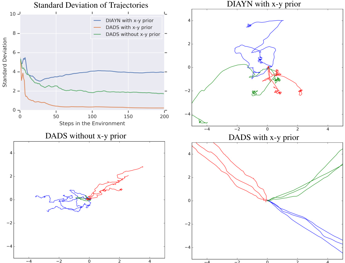
Figure 6: (Top-Left) Standard deviation of Ant’s position as a function of steps in the environment, averaged over multiple skills and normalized by the norm of the position. (Top-Right to Bottom-Left Clockwise) X-Y traces of skills learned using DIAYN with $x{-}y$ prior, DADS with $x{-}y$ prior and DADS without x-y prior, where the same color represents trajectories resulting from the execution of the same skill $z$ in the environment. High variance skills from DIAYN offer limited utility for hierarchical control.

图 6: (左上) 蚂蚁位置的标准差随环境中步数的变化曲线，经多技能平均并按位置范数归一化。(右上至左下顺时针方向) 分别展示使用带$x{-}y$先验的DIAYN、带$x{-}y$先验的DADS以及无$x{-}y$先验的DADS学习到的技能在X-Y平面上的轨迹，同色轨迹表示环境中执行同一技能$z$产生的路径。DIAYN生成的高方差技能在分层控制中实用性有限。

While optimizing for predictability already significantly reduces the variance of the trajectories generated by a primitive, we find that using the $x{-}y$ prior with DADS brings down the skill variance even further. For quantitative benchmarks in the next sections, we assume that the Ant skills are learned using an $x{-}y$ prior on the observation space, for both DADS and DIAYN.

在优化可预测性已显著降低基础动作生成的轨迹方差的基础上，我们发现结合DADS使用$x{-}y$先验能进一步缩小技能方差。针对后续章节的量化基准测试，我们假设Ant技能的学习均采用观测空间的$x{-}y$先验，该方法同时适用于DADS与DIAYN。

6.3 MODEL-BASED REINFORCEMENT LEARNING

6.3 基于模型的强化学习

The key utility of learning a parametric model $q_{\phi}(s^{\prime}|s,z)$ is to take advantage of planning algorithms for downstream tasks, which can be extremely sample-efficient. In our setup, we can solve testtime tasks in zero-shot, that is without any learning on the downstream task. We compare with the state-of-the-art model-based RL method (Chua et al., 2018a), which learns a dynamics model parameterized as $p(s^{\prime}|s,a)$ , on the task of the Ant navigating to a specified goal with a dense reward. Given a goal $g$ , reward at any position $u$ is given by $r(\bar{u})=-|g-\bar{u}|_{2}$ . We benchmark our method against the following variants:

学习参数化模型 $q_{\phi}(s^{\prime}|s,z)$ 的核心价值在于能够利用规划算法处理下游任务，这种方式具有极高的样本效率。在我们的框架中，可以零样本解决测试阶段任务，即无需对下游任务进行任何学习。我们与基于模型的最先进强化学习方法 (Chua et al., 2018a) 进行对比，该方法学习的动态模型参数化为 $p(s^{\prime}|s,a)$ ，测试任务为蚂蚁在密集奖励环境下导航至指定目标。给定目标 $g$ 时，任意位置 $\bar{u}$ 的奖励由 $r(\bar{u})=-|g-\bar{u}|_{2}$ 计算。我们通过以下变体对本方法进行基准测试：

• Random-MBRL (rMBRL): We train the model $p(s^{\prime}|s,a)$ on randomly collected trajectories, and test the zero-shot generalization of the model on a distribution of goals.

• 随机MBRL (rMBRL): 我们在随机收集的轨迹上训练模型 $p(s^{\prime}|s,a)$, 并在目标分布上测试该模型的零样本泛化能力。

• Weak-oracle MBRL (WO-MBRL): We train the model $p(s^{\prime}|s,a)$ on trajectories generated by the planner to navigate to a goal, randomly sampled in every episode. The distribution of goals during training matches the distribution at test time. • Strong-oracle MBRL (SO-MBRL): We train the model $p(s^{\prime}|s,a)$ on a trajectories generated by the planner to navigate to a specific goal, which is fixed for both training and test time.

• 弱预言机MBRL (WO-MBRL)：我们在规划器生成的轨迹上训练模型 $p(s^{\prime}|s,a)$，使智能体能够导航到每轮随机采样的目标。训练期间的目标分布与测试时保持一致。
• 强预言机MBRL (SO-MBRL)：我们在规划器生成的轨迹上训练模型 $p(s^{\prime}|s,a)$，使智能体导航至固定目标，该目标在训练和测试阶段保持不变。

Amongst the variants, only the rMBRL matches our assumptions of having an unsupervised taskagnostic training. Both WO-MBRL and SO-MBRL benefit from goal-directed exploration during training, a significant advantage over DADS, which only uses mutual-information-based exploration.

在众多变体中，只有rMBRL符合我们关于无监督任务无关训练的假设。WO-MBRL和SO-MBRL都受益于训练期间的目标导向探索，这一显著优势超越了仅使用基于互信息探索的DADS。

We use ∆ = PtH=1 H−r(gu)2 as the metric, which represents the distance to the goal g averaged over the episode (wit h the same fixed horizon $H$ for all models and experiments), normalized by the initial distance to the goal $g$ . Therefore, lower $\Delta$ indicates better performance and $0<\Delta\leq1$ (assuming the agent goes closer to the goal). The test set of goals is fixed for all the methods, sampled from $[-15,15]^{2}$ .

我们使用∆ = PtH=1 H−r(gu)2作为指标，它表示在整个回合中到目标g的平均距离（所有模型和实验均采用相同的固定时间范围$H$），并通过初始到目标$g$的距离进行归一化。因此，较低的$\Delta$表示性能更好，且$0<\Delta\leq1$（假设智能体更接近目标）。所有方法的测试目标集均固定，采样自$[-15,15]^{2}$。

Figure 7 demonstrates that the zero-shot planning significantly outperforms all model-based RL baselines, despite the advantage of the baselines being trained on the test goal(s). For the experiment depicted in Figure 7 (Right), DADS has an unsupervised pre-training phase, unlike SO-MBRL which is training directly for the task. A comparison with Random-MBRL shows the significance of mutual-information-based exploration, especially with the right parameter iz ation and priors. This experiment also demonstrates the advantage of learning a continuous space of primitives, which outperforms planning on discrete primitives.

图7表明，零样本规划显著优于所有基于模型的强化学习基线，尽管基线模型在测试目标上经过了训练。在图7(右)所示的实验中，DADS具有无监督预训练阶段，这与直接针对任务进行训练的SO-MBRL不同。与Random-MBRL的对比显示了基于互信息探索的重要性，特别是在正确的参数化和先验条件下。该实验还证明了学习连续基元空间的优势，其性能优于离散基元上的规划。

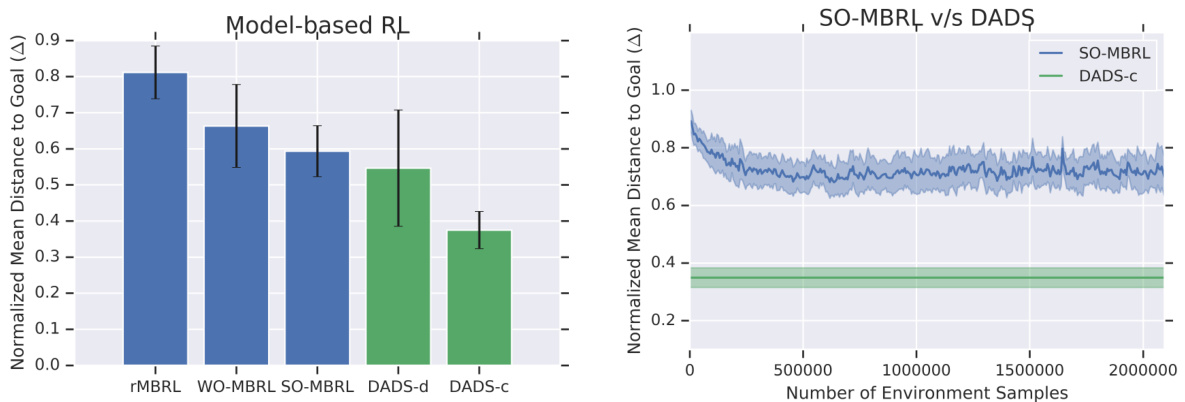
Figure 7: (Left) The results of the MPPI controller on skills learned using DADS-c (continuous primitives) and DADS-d (discrete primitives) significantly outperforms state-of-the-art model-based RL. (Right) Planning for a new task does not require any additional training and outperforms model-based RL being trained for the specific task.

图 7: (左) 使用DADS-c(连续基元)和DADS-d(离散基元)学习技能后，MPPI控制器的结果显著优于最先进的基于模型的强化学习。(右) 针对新任务的规划无需任何额外训练，其表现优于针对特定任务训练的基于模型的强化学习。

6.4 HIERARCHICAL CONTROL WITH UNSUPERVISED PRIMITIVES

6.4 基于无监督基元的层次化控制

We benchmark hierarchical control for primitives learned without supervision, against our proposed scheme using an MPPI based planner on top of DADS-learned skills. We persist with the task of Ant-navigation as described in 6.3. We benchmark against Hierarchical DIAYN (Eysenbach et al., 2018), which learns the skills using the DIAYN objective, freezes the low-level policy and learns a meta-controller that outputs the skill to be executed for the next $H_{Z}$ steps. We provide the $x{-}y$ prior to the DIAYN’s disc imina tor while learning the skills for the Ant agent. The performance of the meta-controller is constrained by the low-level policy, however, this hierarchical scheme is agnostic to the algorithm used to learn the low-level policy. To contrast the quality of primitives learned by the DADS and DIAYN, we also benchmark against Hierarchical DADS, which learns a meta-controller the same way as Hierarchical DIAYN, but learns the skills using DADS.

我们对无监督学习的原始分层控制进行了基准测试，并与我们提出的方案进行了对比。我们的方案在DADS学习技能的基础上使用了基于MPPI的规划器。我们延续了6.3节中描述的蚂蚁导航任务。我们以分层DIAYN (Eysenbach et al., 2018) 作为基准，该方法通过DIAYN目标学习技能，冻结底层策略并学习一个元控制器，该控制器输出接下来 $H_{Z}$ 步要执行的技能。在为蚂蚁智能体学习技能时，我们向DIAYN的判别器提供了 $x{-}y$ 先验。元控制器的性能受限于底层策略，但该分层方案对学习底层策略的算法是不可知的。为了对比DADS和DIAYN学习的原始技能质量，我们还以分层DADS作为基准，该方法与分层DIAYN学习元控制器的方式相同，但使用DADS学习技能。

From Figure 8 (Left) We find that the meta-controller is unable to compose the skills learned by DIAYN, while the same meta-controller can learn to compose skills by DADS to navigate the Ant to different goals. This result seems to confirm our intuition described in Section 6.2, that the high variance of the DIAYN skills limits their temporal compositional it y. Interestingly, learning a RL meta-controller reaches similar performance to the MPPI controller, taking an additional 200, 000 samples per goal.

从图 8 (左) 我们发现元控制器无法组合 DIAYN 学习的技能，而相同的元控制器可以通过组合 DADS 学习的技能来引导 Ant 到达不同目标。这一结果似乎验证了我们在 6.2 节的直觉：DIAYN 技能的高方差性限制了其时间组合能力。值得注意的是，学习 RL 元控制器达到了与 MPPI 控制器相近的性能，但每个目标需要额外采样 200, 000 次。

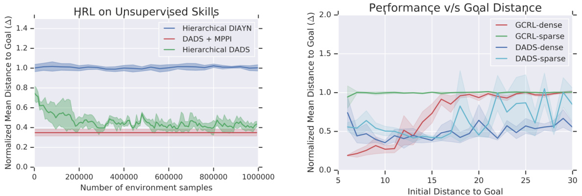
Figure 8: (Left) A RL-trained meta-controller is unable to compose primitive learned by DIAYN to navigate Ant to a goal, while it succeeds to do so using the primitives learned by DADS. (Right) Goal-Conditioned RL (GCRL-dense/sparse) does not generalize outside its training distribution, while MPPI controller on learned skills (DADS-dense/sparse) experiences significantly smaller degrade in performance.

图 8: (左) 经过强化学习训练的元控制器无法组合由DIAYN习得的原始动作来引导Ant到达目标，而使用DADS学习的原始动作则能成功实现。(右) 目标条件强化学习(GCRL-dense/sparse)在训练分布之外无法泛化，而基于习得技能的MPPI控制器(DADS-dense/sparse)性能下降幅度显著更小。

6.5 GOAL-CONDITIONED RL

6.5 目标条件强化学习

To demonstrate the benefits of our approach over model-free RL, we benchmark against goalconditioned RL on two versions of Ant-navigation: (a) with a dense reward $r(u)$ and (b) with a sparse reward $r(u)=1$ if $|u-g|_{2}\leq\epsilon$ , else 0. We train the goal-conditioned RL agent using soft actor-critic, where the state variable of the agent is augmented with $u-g$ , the position delta to the goal. The agent gets a randomly sampled goal from $[-10,10]^{2}$ at the beginning of the episode.

为了展示我们的方法相较于无模型强化学习(RL)的优势，我们在两种版本的蚂蚁导航任务上对目标条件强化学习进行了基准测试：(a) 使用密集奖励 $r(u)$ ，(b) 使用稀疏奖励 $r(u)=1$ （当 $|u-g|_{2}\leq\epsilon$ 时），否则为0。我们采用软演员-评论家算法训练目标条件强化学习智能体，其状态变量通过目标位置差 $u-g$ 进行扩展。每轮训练开始时，智能体会从 $[-10,10]^{2}$ 范围内随机采样一个目标。

In Figure 8 (Right), we measure the average performance of the all the methods as a function of the initial distance of the goal, ranging from 5 to 30 metres. For dense reward navigation, we observe that while model-based planning on DADS-learned skills degrades smoothly as the initial distance to goal to increases, goal-conditioned RL experiences a sudden deterioration outside the goal distribution it was trained on. Even within the goal distribution observed during training of goal-conditioned RL model, skill-space planning performs competitively to it. With sparse reward navigation, goal-conditioned RL is unable to navigate, while MPPI demonstrates comparable performance to the dense reward up to about 20 metres. This highlights the utility of learning task-agnostic skills, which makes them more general while showing that latent space planning can be leveraged for tasks requiring long-horizon planning.

在图 8 (右) 中，我们测量了所有方法的平均性能随目标初始距离 (5 至 30 米) 的变化情况。对于密集奖励导航，我们观察到基于 DADS 学习技能的模型规划性能会随着目标初始距离的增加而平稳下降，而目标条件强化学习 (goal-conditioned RL) 在训练目标分布之外会出现突然的性能恶化。即使在目标条件强化学习模型的训练目标分布范围内，技能空间规划的表现也与其相当。在稀疏奖励导航中，目标条件强化学习无法完成导航任务，而 MPPI 在 20 米范围内的表现与密集奖励相当。这凸显了学习任务无关技能的优势：它们更具通用性，同时表明潜空间规划可用于需要长程规划的任务。

7 CONCLUSION

7 结论

We have proposed a novel unsupervised skill learning algorithm that is amenable to model-based planning for hierarchical control on downstream tasks. We show that our skill learning method can scale to high-dimensional state-spaces, while discovering a diverse set of low-variance skills. In addition, we demonstrated that, without any training on the specified task, we can compose the learned skills to outperform competitive model-based baselines that were trained with the knowledge of the test tasks. We plan to extend the algorithm to work with off-policy data, potentially using relabelling tricks (An dry ch owicz et al., 2017; Nachum et al., 2018) and explore more nuanced planning algorithms. We plan to apply the hereby-introduced method to different domains, such as manipulation and enable skill/model discovery directly from images.

我们提出了一种新颖的无监督技能学习算法，该算法适用于下游任务分层控制的基于模型的规划。我们证明，我们的技能学习方法能够扩展到高维状态空间，同时发现一组多样化的低方差技能。此外，我们还展示了，在未对指定任务进行任何训练的情况下，我们可以组合所学技能，以超越那些在测试任务知识基础上训练的基于模型的竞争基线。我们计划将该算法扩展到适用于离策略数据，可能会使用重新标记技巧 (An dry ch owicz et al., 2017; Nachum et al., 2018)，并探索更细致的规划算法。我们计划将本文提出的方法应用于不同领域，例如操作任务，并直接从图像中实现技能/模型发现。

8 ACKNOWLEDGEMENTS

8 致谢

We would like to thank Evan Liu, Ben Eysenbach, Anusha Nagabandi for their help in reproducing the baselines for this work. We are thankful to Ben Eysenbach for their comments and discussion on the initial drafts. We would also like to acknowledge Ofir Nachum, Alex Alemi, Daniel Freeman, Yiding Jiang, Allan Zhou and other colleagues at Google Brain for their helpful feedback and discussions at various stages of this work. We are also thankful to Michael Ahn and others in Adept team for their support, especially with the infrastructure setup and scaling up the experiments.

我们要感谢Evan Liu、Ben Eysenbach和Anusha Nagabandi在复现本工作基线时提供的帮助。感谢Ben Eysenbach对初稿提出的意见与讨论。同时，我们也要感谢Ofir Nachum、Alex Alemi、Daniel Freeman、Yiding Jiang、Allan Zhou以及Google Brain的其他同事在本工作各个阶段给予的有益反馈和讨论。此外，特别感谢Michael Ahn及Adept团队其他成员的支持，尤其是在基础设施搭建和实验扩展方面提供的帮助。

REFERENCES

参考文献

Benjamin Eysenbach, Abhishek Gupta, Julian Ibarz, and Sergey Levine. Diversity is all you need: Learning skills without a reward function. arXiv preprint arXiv:1802.06070, 2018.

Benjamin Eysenbach、Abhishek Gupta、Julian Ibarz 和 Sergey Levine。《多样性即所需：无需奖励函数学习技能》。arXiv预印本 arXiv:1802.06070，2018年。

Carlos Florensa, Yan Duan, and Pieter Abbeel. Stochastic neural networks for hierarchical reinforcement learning. arXiv preprint arXiv:1704.03012, 2017.

Carlos Florensa、Yan Duan 和 Pieter Abbeel。用于分层强化学习的随机神经网络。arXiv预印本 arXiv:1704.03012，2017。

Nir Friedman, Ori Mosenzon, Noam Slonim, and Naftali Tishby. Multivariate information bottleneck. In Proceedings of the Seventeenth conference on Uncertainty in artificial intelligence, pp. 152–161. Morgan Kaufmann Publishers Inc., 2001.

Nir Friedman、Ori Mosenzon、Noam Slonim 和 Naftali Tishby。多元信息瓶颈 (Multivariate Information Bottleneck)。载于《第十七届人工智能不确定性会议论文集》第152-161页。Morgan Kaufmann出版社，2001年。

Justin Fu, Sergey Levine, and Pieter Abbeel. One-shot learning of manipulation skills with online dynamics adaptation and neural network priors. In 2016 IEEE/RSJ International Conference on Intelligent Robots and Systems (IROS), pp. 4019–4026. IEEE, 2016.

Justin Fu、Sergey Levine 和 Pieter Abbeel。基于在线动态适应与神经网络先验的单次操作技能学习。收录于 2016 年 IEEE/RSJ 智能机器人与系统国际会议 (IROS)，第 4019–4026 页。IEEE，2016。

Justin Fu, John Co-Reyes, and Sergey Levine. Ex2: Exploration with exemplar models for deep reinforcement learning. In I. Guyon, U. V. Luxburg, S. Bengio, H. Wallach, R. Fergus, S. Vishwanath an, and R. Garnett (eds.), Advances in Neural Information Processing Systems 30, pp. 2577–2587. Curran Associates, Inc., 2017. URL http://papers.nips.cc/paper/ 6851-ex2-exploration-with-exemplar-models-for-deep-reinforcement-learning. pdf.

Justin Fu、John Co-Reyes 和 Sergey Levine。EX2：基于范例模型的深度强化学习探索。载于 I. Guyon、U. V. Luxburg、S. Bengio、H. Wallach、R. Fergus、S. Vishwanath an 和 R. Garnett (编) ，《神经信息处理系统进展 30》，第 2577–2587 页。Curran Associates 公司，2017。URL http://papers.nips.cc/paper/6851-ex2-exploration-with-exemplar-models-for-deep-reinforcement-learning.pdf。

Yarin Gal, Rowan McAllister, and Carl Edward Rasmussen. Improving pilco with bayesian neural network dynamics models. In Data-Efficient Machine Learning workshop, ICML, volume 4, 2016.

Yarin Gal、Rowan McAllister 和 Carl Edward Rasmussen。利用贝叶斯神经网络动力学模型改进 PILCO。收录于《数据高效机器学习研讨会》，ICML，第4卷，2016年。

Carlos E Garcia, David M Prett, and Manfred Morari. Model predictive control: theory and practicea survey. Automatica, 25(3):335–348, 1989.

Carlos E Garcia、David M Prett 和 Manfred Morari。模型预测控制：理论与实践的综述。Automatica, 25(3):335–348, 1989.

Karol Gregor, Danilo Jimenez Rezende, and Daan Wierstra. Variation al intrinsic control. arXiv preprint arXiv:1611.07507, 2016.

Karol Gregor、Danilo Jimenez Rezende 和 Daan Wierstra. 变分内在控制. arXiv 预印本 arXiv:1611.07507, 2016.

Shixiang Gu, Ethan Holly, Timothy Lillicrap, and Sergey Levine. Deep reinforcement learning for robotic manipulation with asynchronous off-policy updates. In 2017 IEEE International Conference on Robotics and Automation (ICRA), pp. 3389–3396. IEEE, 2017.

Shixiang Gu、Ethan Holly、Timothy Lillicrap和Sergey Levine。基于异步离策略更新的机器人操作深度强化学习。发表于《2017年IEEE机器人与自动化国际会议(ICRA)》，第3389-3396页。IEEE，2017年。

David Ha and Juirgen Schmid huber. Recurrent world models facilitate policy evolution. In Advances in Neural Information Processing Systems, pp. 2455–2467, 2018.

David Ha 和 Juirgen Schmidhuber. 循环世界模型促进策略进化. 载于《神经信息处理系统进展》, 第2455–2467页, 2018.

Tuomas Haarnoja, Aurick Zhou, Pieter Abbeel, and Sergey Levine. Soft actor-critic: Off- policy maximum entropy deep reinforcement learning with a stochastic actor. arXiv preprint arXiv:1801.01290, 2018a.

Tuomas Haarnoja, Aurick Zhou, Pieter Abbeel, 和 Sergey Levine. Soft actor-critic: 随机行动者的离策略最大熵深度强化学习. arXiv预印本 arXiv:1801.01290, 2018a.

Tuomas Haarnoja, Aurick Zhou, Kristian Hart ika inen, George Tucker, Sehoon Ha, Jie Tan, Vikash Kumar, Henry Zhu, Abhishek Gupta, Pieter Abbeel, and Sergey Levine. Soft actor-critic algorithms and applications. CoRR, abs/1812.05905, 2018b. URL http://arxiv.org/abs/ 1812.05905.

Tuomas Haarnoja、Aurick Zhou、Kristian Hartikainen、George Tucker、Sehoon Ha、Jie Tan、Vikash Kumar、Henry Zhu、Abhishek Gupta、Pieter Abbeel 和 Sergey Levine。Soft actor-critic算法与应用。CoRR, abs/1812.05905, 2018b。URL http://arxiv.org/abs/1812.05905。

Karol Hausman, Jost Tobias Spring e nberg, Ziyu Wang, Nicolas Heess, and Martin Riedmiller. Learning an embedding space for transferable robot skills. In International Conference on Learning Representations, 2018. URL https://openreview.net/forum?id $\equiv$ rk07ZXZRb.

Karol Hausman、Jost Tobias Springenberg、Ziyu Wang、Nicolas Heess 和 Martin Riedmiller。学习可迁移机器人技能的嵌入空间。收录于国际学习表征会议，2018年。URL https://openreview.net/forum?id $\equiv$ rk07ZXZRb。

Nicolas Heess, Greg Wayne, Yuval Tassa, Timothy Lillicrap, Martin Riedmiller, and David Silver. Learning and transfer of modulated locomotor controllers. arXiv preprint arXiv:1610.05182, 2016.

Nicolas Heess、Greg Wayne、Yuval Tassa、Timothy Lillicrap、Martin Riedmiller 和 David Silver。调制运动控制器的学习与迁移。arXiv预印本 arXiv:1610.05182，2016。

Nicolas Heess, Srinivasan Sriram, Jay Lemmon, Josh Merel, Greg Wayne, Yuval Tassa, Tom Erez, Ziyu Wang, SM Eslami, Martin Riedmiller, et al. Emergence of locomotion behaviours in rich environments. arXiv preprint arXiv:1707.02286, 2017.

Nicolas Heess, Srinivasan Sriram, Jay Lemmon, Josh Merel, Greg Wayne, Yuval Tassa, Tom Erez, Ziyu Wang, SM Eslami, Martin Riedmiller, 等. 丰富环境中运动行为的涌现. arXiv预印本 arXiv:1707.02286, 2017.

Rein Houthooft, Xi Chen, Yan Duan, John Schulman, Filip De Turck, and Pieter Abbeel. Curiosity-driven exploration in deep reinforcement learning via bayesian neural networks. CoRR, abs/1605.09674, 2016. URL http://arxiv.org/abs/1605.09674.

Rein Houthooft、Xi Chen、Yan Duan、John Schulman、Filip De Turck 和 Pieter Abbeel。基于贝叶斯神经网络 (Bayesian Neural Networks) 的深度强化学习好奇心驱动探索。CoRR, abs/1605.09674, 2016。URL http://arxiv.org/abs/1605.09674。

Robert A Jacobs, Michael I Jordan, Steven J Nowlan, Geoffrey E Hinton, et al. Adaptive mixtures of local experts. Neural computation, 3(1):79–87, 1991.

Robert A Jacobs、Michael I Jordan、Steven J Nowlan、Geoffrey E Hinton 等。自适应局部专家混合。Neural computation, 3(1):79–87, 1991。

Dmitry Kalashnikov, Alex Irpan, Peter Pastor, Julian Ibarz, Alexander Herzog, Eric Jang, Deirdre Quillen, Ethan Holly, Mrinal Kala krishna n, Vincent Vanhoucke, et al. Qt-opt: Scalable deep reinforcement learning for vision-based robotic manipulation. arXiv preprint arXiv:1806.10293, 2018.

Dmitry Kalashnikov、Alex Irpan、Peter Pastor、Julian Ibarz、Alexander Herzog、Eric Jang、Deirdre Quillen、Ethan Holly、Mrinal Kalakrishnan、Vincent Vanhoucke等。Qt-opt: 可扩展的深度强化学习在基于视觉的机器人操作中的应用。arXiv预印本 arXiv:1806.10293, 2018。

Pierre-Yves Oudeyer, Frdric Kaplan, and Verena V Hafner. Intrinsic motivation systems for au

Pierre-Yves Oudeyer、Frdric Kaplan 和 Verena V Hafner。自主行为的内在动机系统

Emanuel Todorov, Tom Erez, and Yuval Tassa. Mujoco: A physics engine for model-based control. In 2012 IEEE/RSJ International Conference on Intelligent Robots and Systems, pp. 5026–5033. IEEE, 2012.

Emanuel Todorov、Tom Erez 和 Yuval Tassa。Mujoco: 基于模型控制的物理引擎。收录于2012年IEEE/RSJ智能机器人与系统国际会议论文集，第5026–5033页。IEEE，2012年。

Alexander Sasha Vezhnevets, Simon Osindero, Tom Schaul, Nicolas Heess, Max Jaderberg, David Silver, and Koray Ka vuk cuo g lu. Feudal networks for hierarchical reinforcement learning. In Proceedings of the 34th International Conference on Machine Learning-Volume 70, pp. 3540– 3549. JMLR. org, 2017.

Alexander Sasha Vezhnevets、Simon Osindero、Tom Schaul、Nicolas Heess、Max Jaderberg、David Silver 和 Koray Kavukcuoglu。用于分层强化学习的封建网络 (Feudal Networks)。见《第34届国际机器学习会议论文集》第70卷，第3540–3549页。JMLR.org，2017年。

David Warde-Farley, Tom Van de Wiele, Tejas Kulkarni, Catalin Ionescu, Steven Hansen, and Volodymyr Mnih. Unsupervised control through non-parametric disc rim i native rewards. arXiv preprint arXiv:1811.11359, 2018.

David Warde-Farley、Tom Van de Wiele、Tejas Kulkarni、Catalin Ionescu、Steven Hansen 和 Volodymyr Mnih。基于非参数判别奖励的无监督控制。arXiv预印本 arXiv:1811.11359，2018。

Manuel Watter, Jost Spring e nberg, Joschka Boedecker, and Martin Riedmiller. Embed to control: A locally linear latent dynamics model for control from raw images. In Advances in neural information processing systems, pp. 2746–2754, 2015.

Manuel Watter、Jost Springenberg、Joschka Boedecker 和 Martin Riedmiller。从原始图像到控制：一种局部线性潜在动力学模型。载于《神经信息处理系统进展》，第2746-2754页，2015年。

Grady Williams, Paul Drews, Brian Goldfain, James M Rehg, and Evangelos A Theodorou. Aggressive driving with model predictive path integral control. In 2016 IEEE International Conference on Robotics and Automation (ICRA), pp. 1433–1440. IEEE, 2016.

Grady Williams、Paul Drews、Brian Goldfain、James M Rehg 和 Evangelos A Theodorou。基于模型预测路径积分控制的激进驾驶。载于《2016年IEEE机器人与自动化国际会议(ICRA)》，第1433-1440页。IEEE，2016年。

A IMPLEMENTATION DETAILS

实现细节

All of our models are written in the open source Tensorflow-Agents (Sergio Guadarrama, Anoop Ko ratti kara, Oscar Ramirez, Pablo Castro, Ethan Holly, Sam Fishman, Ke Wang, Ekaterina Gonina, Chris Harris, Vincent Vanhoucke, Eugene Brevdo, 2018), based on Tensorflow (Abadi et al., 2015).

我们所有的模型均基于 Tensorflow (Abadi et al., 2015) ，采用开源框架 Tensorflow-Agents (Sergio Guadarrama, Anoop Korattikara, Oscar Ramirez, Pablo Castro, Ethan Holly, Sam Fishman, Ke Wang, Ekaterina Gonina, Chris Harris, Vincent Vanhoucke, Eugene Brevdo, 2018) 实现。

A.1 SKILL SPACES

A.1 技能空间

When using discrete spaces, we parameter ize $\mathcal{Z}$ as one-hot vectors. These one-hot vectors are randomly sampled from the uniform prior $\textstyle p(z)={\frac{1}{D}}$ , where $D$ is the number of skills. We experiment with $D\leq128$ . For discrete skills learnt for MuJoCo Ant in Section 6.3, we use $D=20$ . For continuous spaces, we sample $z\sim\mathrm{Uniform}(-1,1)^{D}$ . We experiment with $D=2$ for Ant learnt with x-y prior, $D=3$ for Ant learnt without x-y prior (that is full observation space), to $D=5$ for Humanoid on full observation spaces. The skills are sampled once in the beginning of the episode and fixed for the rest of the episode. However, it is possible to resample the skill from the prior within the episode, which allows for every skill to experience a different distribution than the initi aliz ation distribution. This also encourages discovery of skills which can be composed temporally. However, this increases the hardness of problem, especially if the skills are re-sampled from the prior frequently.

在使用离散空间时，我们将$\mathcal{Z}$参数化为独热向量 (one-hot vectors)。这些独热向量从均匀先验$\textstyle p(z)={\frac{1}{D}}$中随机采样，其中$D$表示技能数量。我们实验了$D\leq128$的情况。在第6.3节为MuJoCo Ant学习的离散技能中，我们使用$D=20$。对于连续空间，我们采样$z\sim\mathrm{Uniform}(-1,1)^{D}$。我们实验了从$x-y$先验学习的Ant使用$D=2$，无$x-y$先验（即完整观察空间）学习的Ant使用$D=3$，到完整观察空间下Humanoid使用$D=5$的情况。技能在每轮开始时采样一次并在该轮剩余时间内固定。然而，也可以在轮次内从先验重新采样技能，这使得每个技能能经历不同于初始化的分布。这也鼓励发现可以随时间组合的技能。但这样做会增加问题难度，尤其是当技能频繁从先验重新采样时。

A.2 AGENT

A.2 通用人工智能 (AGI)

We use SAC as the optimizer for our agent $\pi(a\mid s,z)$ , in particular, EC-SAC (Haarnoja et al., 2018b). The $s$ input to the policy generally excludes global co-ordinates $(x,y)$ of the centre-ofmass, available for a lot of en vi rome nts in OpenAI gym, which helps produce skills agnostic to the location of the agent. We restrict to two hidden layers for our policy and critic networks. However, to improve the expressivity of skills, it is beneficial to increase the capacity of the networks. The hidden layer sizes can vary from (128, 128) for Half-Cheetah to (512, 512) for Ant and (1024, 1024) for Humanoid. The critic $Q(s,a,z)$ is similarly parameterized. The target function for critic $Q$ is updated every iteration using a soft updates with co-efficient of 0.005. We use Adam (Kingma & Ba, 2014) optimizer with a fixed learning rate of $3e-4$ , and a fixed initial entropy co-efficient $\beta=0.1$ . While the policy is parameterized as a normal distribution $\mathcal{N}(\mu(s,z),\Sigma(s,z))$ where $\Sigma$ is a diagonal covariance matrix, it undergoes through tanh transformation, to transform the output to the range $(-1,1)$ and constrain to the action bounds.

我们采用SAC作为智能体$\pi(a\mid s,z)$的优化器，具体来说是EC-SAC (Haarnoja et al., 2018b)。策略的输入$s$通常不包含质心的全局坐标$(x,y)$（该信息在OpenAI gym的许多环境中可用），这有助于生成与智能体位置无关的技能。我们将策略网络和评论家网络的隐藏层限制为两层，但为了提高技能的表达能力，增加网络容量是有益的。隐藏层大小从Half-Cheetah的(128, 128)到Ant的(512, 512)以及Humanoid的(1024, 1024)不等。评论家$Q(s,a,z)$采用类似的参数化方式，其目标函数每次迭代通过系数为0.005的软更新进行更新。我们使用Adam (Kingma & Ba, 2014)优化器，固定学习率为$3e-4$，初始熵系数固定为$\beta=0.1$。策略参数化为正态分布$\mathcal{N}(\mu(s,z),\Sigma(s,z))$，其中$\Sigma$为对角协方差矩阵，并经过tanh变换将输出范围转换至$(-1,1)$以符合动作边界约束。

A.3 SKILL-DYNAMICS

A.3 技能动态 (SKILL-DYNAMICS)

Skill-dynamics, denoted by $q(s^{\prime}\mid s,z)$ , is parameterized by a deep neural network. A common trick in model-based RL is to predict the $\Delta s=s^{\prime}-s$ , rather than the full state $s^{\prime}$ . Hence, the prediction network is $q(\Delta s\mid s,z)$ . Note, both parameter iz at ions can represent the same set of functions. However, the latter will be easy to learn as $\Delta s$ will be centred around 0. We exclude the global coordinates from from the state input to $q$ . However, we can (and we still do) predict $\Delta_{x},\Delta_{y}$ , because reward functions for goal-based navigation generally rely on the position prediction from the model. This represents another benefit of predicting state-deltas, as we can still predict changes in position without explicitly knowing the global position.

技能动态学，用 $q(s^{\prime}\mid s,z)$ 表示，通过深度神经网络参数化。基于模型的强化学习中常见技巧是预测 $\Delta s=s^{\prime}-s$ 而非完整状态 $s^{\prime}$，因此预测网络为 $q(\Delta s\mid s,z)$。需注意，这两种参数化方式可表示相同的函数集，但后者更易学习，因为 $\Delta s$ 会以0为中心分布。我们将全局坐标从 $q$ 的状态输入中排除，但仍可（且实际仍在）预测 $\Delta_{x},\Delta_{y}$，因为基于目标的导航任务通常依赖模型的位置预测。这体现了预测状态增量的另一优势：即便不明确知晓全局位置，仍能预测位置变化。

The output distribution is modelled as a Mixture-of-Experts (Jacobs et al., 1991). We fix the number of experts to be 4. We model each expert as a Gaussian distribution. The input $(s,z)$ goes through two hidden layers (the same capacity as that of policy and critic networks, for example (512, 512) for Ant). The output of the two hidden layers is used as an input to the mixture-of-experts, which is linearly transformed to output the parameters of the Gaussian distribution, and a discrete distribution over the experts using a softmax distribution. In practice, we fix the covariance matrix of the Gaussian experts to be an identity matrix, so we only need to output the means for the experts. We use batch-normalization for both input and the hidden layers. We normalize the output targets using their batch-average and batch-standard deviation, similar to batch-normalization.

输出分布被建模为专家混合模型 (Mixture-of-Experts) (Jacobs et al., 1991)。我们将专家数量固定为4，并将每个专家建模为高斯分布。输入 $(s,z)$ 经过两个隐藏层（与策略网络和评论网络的容量相同，例如Ant任务中为(512, 512)）。这两个隐藏层的输出作为专家混合模型的输入，通过线性变换输出高斯分布的参数，并使用softmax分布输出专家离散分布。实际应用中，我们将高斯专家的协方差矩阵固定为单位矩阵，因此只需输出专家的均值。我们对输入和隐藏层使用批量归一化 (batch-normalization)，并使用批平均和批标准差对输出目标进行归一化，类似于批量归一化的操作。

A.4 OTHER HYPER PARAMETERS

A.4 其他超参数

The episode horizon is generally kept shorter for stable agents like Ant (200), while longer for unstable agents like Humanoid (1000). For Ant, longer episodes do not add value, but Humanoid can benefit from longer episodes as it helps it filter skills which are unstable. The optimization scheme is on-policy, and we collect 2000 steps for Ant and 4000 steps for Humanoid in one iteration. The intuition is to experience trajectories generated by multiple skills (approximately 10) in a batch. Re-sampling skills can enable experiencing larger number of skills. Once a batch of episodes is collected, the skill-dynamics is updated using Adam optimizer with a fixed learning rate of $3e-4$ . The batch size is 128, and we carry out 32 steps of gradient descent. To compute the intrinsic reward, we need to resample the prior for computing the denominator. For continuous spaces, we set $L=500$ . For discrete spaces, we can marginal ize over all skills. After the intrinsic reward is computed, the policy and critic networks are updated for 128 steps with a batch size of 128. The intuition is to ensure that every sample in the batch is seen for policy and critic updates about $3-4$ times in expectation.

对于稳定智能体如Ant (200)，通常将回合时长设得较短，而不稳定智能体如Humanoid (1000)则采用较长回合。Ant的较长回合并无增益，但Humanoid能通过延长回合过滤不稳定技能。优化方案采用同策略(on-policy)，每轮迭代收集2000步(Ant)和4000步(Humanoid)数据，旨在单批次内体验约10种技能生成的轨迹。通过重采样技能可接触更多技能组合。收集整批回合数据后，使用固定学习率$3e-4$的Adam优化器更新技能动力学，批大小为128并执行32步梯度下降。计算内在奖励时需对先验分布重采样求得分母项：连续空间设$L=500$，离散空间则对所有技能求边际分布。计算完内在奖励后，策略网络与评价网络以128批大小更新128步，确保批次样本在策略和评价更新中平均被处理$3-4$次。

A.5 PLANNING AND EVALUATION SETUPS

A.5 规划与评估设置

For evaluation, we fix the episode horizon to 200 for all models in all evaluation setups. Depending upon the size of the latent space and planning horizon, the number of samples from the planning distribution $P$ is varied between $10-200$ . For $H_{P}=1,H_{Z}=10$ and a $2D$ latent space, we use 50 samples from the planning distribution $P$ . The co-efficient $\gamma$ for MPPI is fixed to 10. We use a setting of $H_{P}=1$ and $H_{Z}=10$ for dense-reward navigation, in which case we set the number of refine steps $R=10$ . However, for sparse reward navigation it is important to have a longer horizon planning, in which case we set $H_{P}=4,H_{Z}=25$ with a higher number of samples from the planning distribution (200 from $P$ ). Also, when using longer planning horizons, we found that smoothing the sampled plans help. Thus, if the sampled plan is $z_{1},z_{2},z_{3},z_{4}...,$ we smooth the plan to make $\dot{z_{2}}=\beta z_{1}\dot{+}(1-\beta)z_{2}$ and so on, with $\beta=0.9$ .

在评估阶段，我们将所有模型在所有评估设置中的每轮步长固定为200步。根据潜在空间大小和规划范围的不同，从规划分布$P$中采样的样本数量在$10-200$之间变化。对于$H_{P}=1,H_{Z}=10$的二维潜在空间，我们从规划分布$P$中抽取50个样本。MPPI算法的系数$\gamma$固定为10。在密集奖励导航任务中，我们采用$H_{P}=1$和$H_{Z}=10$的参数配置，此时设定优化步数$R=10$。但对于稀疏奖励导航任务，采用更长规划范围至关重要，因此我们设置$H_{P}=4,H_{Z}=25$并从规划分布$P$中抽取更多样本（200个）。此外，当使用较长规划范围时，我们发现平滑采样计划能提升效果。具体而言，若采样计划为$z_{1},z_{2},z_{3},z_{4}...,$，则通过$\dot{z_{2}}=\beta z_{1}\dot{+}(1-\beta)z_{2}$等方式平滑处理（其中$\beta=0.9$），后续节点依此类推。

For hierarchical controllers being learnt on top of low-level unsupervised primitives, we use PPO (Schulman et al., 2017) for discrete action skills, while we use SAC for continuous skills. We keep the number of steps after which the meta-action is decided as 10 (that is $H_{Z}=10$ ). The hidden layer sizes of the meta-controller are (128, 128). We use a learning rate of 1e-4 for PPO and 3e-4 for SAC.

对于在低层无监督基元之上学习的分层控制器，我们使用PPO (Schulman等人，2017) 来训练离散动作技能，而使用SAC来训练连续技能。我们将元动作决策间隔步数保持为10 (即 $H_{Z}=10$ )。元控制器的隐藏层大小为(128, 128)。PPO的学习率设为 1e-4，SAC的学习率设为 3e-4 。

For our model-based RL baseline PETS, we use an ensemble size of 3, with a fixed planning horizon of 20. For the model, we use a neural network with two hidden layers of size 400. In our experiments, we found that MPPI outperforms CEM, so we report the results using the MPPI as our controller.

对于我们基于模型的强化学习基线方法PETS，我们使用包含3个模型的集成，并固定规划时域为20步。模型结构采用具有两个隐藏层（每层400个节点）的神经网络。实验发现MPPI控制器的性能优于CEM，因此最终采用MPPI作为控制器汇报结果。

B GRAPHICAL MODELS, INFORMATION BOTTLENECK AND UNSUPERVISED SKILL LEARNING

B 图模型、信息瓶颈与无监督技能学习

We now present a novel perspective on unsupervised skill learning, motivated from the literature on information bottleneck. This section takes inspiration from (Alemi & Fischer, 2018), which helps us provide a rigorous justification for our objective proposed earlier. To obtain our unsupervised RL objective, we setup a graphical model $P$ as shown in Figure 9, which represents the distribution of trajectories generated by a given policy $\pi$ . The joint distribution is given by:

我们现在从信息瓶颈 (information bottleneck) 文献中获得启发，提出一种无监督技能学习的新视角。本节借鉴了 (Alemi & Fischer, 2018) 的研究，为我们先前提出的目标提供了严格的理论依据。为了推导无监督强化学习目标，我们建立了如图 9 所示的概率图模型 $P$ ，它表示给定策略 $\pi$ 生成轨迹的分布。联合分布由以下公式给出:

$$
p(s_{1},a_{1}\ldots a_{T-1},s_{T},z)=p(z)p(s_{1})\prod_{t=1}^{T-1}\pi(a_{t}|s_{t},z)p(s_{t+1}|s_{t},a_{t}).
$$

Figure 9: Graphical model for the world $P$ in which the trajectories are generated while interacting with the environment. Shaded nodes represent the distributions we optimize.

图 9: 轨迹在与环境交互时生成的世界 $P$ 的图形模型。阴影节点表示我们优化的分布。

Figure 10: Graphical model for the world $N$ which is the desired representation of the world.

图 10: 世界 $N$ 的图模型，这是世界的理想表示形式。

We setup another graphical model $N$ , which represents the desired model of the world. In particular, we are interested in approximating $p(s^{\prime}|s,z)$ , which represents the transition function for a particular primitive. This abstraction helps us get away from knowing the exact actions, enabling model-based planning in behavior space (as discussed in the main paper). The joint distribution for $N$ shown in Figure 10 is given by:

我们建立了另一个图形模型 $N$，它表示期望的世界模型。具体而言，我们关注近似 $p(s^{\prime}|s,z)$，这代表特定基元的转移函数。这种抽象使我们无需了解具体动作，从而实现在行为空间中进行基于模型的规划（如主论文所述）。图 10 中 $N$ 的联合分布由下式给出：

$$
\eta(s_{1},a_{1},\ldots s_{T},a_{T},z)=\eta(z)\eta(s_{1})\prod_{t=1}^{T-1}\eta(a_{t})\eta(s_{t+1}|s_{t},z).
$$

The goal of our approach is to optimize the distribution $\pi(\boldsymbol{a}|\boldsymbol{s},\boldsymbol{z})$ in the graphical model $P$ to minimize the distance between the two distributions, when transforming to the representation of the graphical model $Z$ . In particular, we are interested in minimizing the KL divergence between $p$ and $\eta$ , that is $\mathcal{D}_{K L}(p||\eta)$ . Note, if $N$ had the same structure as $P$ , the information lost in projection would be 0 for any valid $P$ . Interestingly, we can exploit the following result from in Friedman et al. (2001) to setup the objective for $\pi$ , without explicitly knowing $\eta$ :

我们方法的目标是优化图模型 $P$ 中的分布 $\pi(\boldsymbol{a}|\boldsymbol{s},\boldsymbol{z})$，以最小化在转换为图模型 $Z$ 表示时两个分布之间的距离。具体而言，我们希望最小化 $p$ 和 $\eta$ 之间的KL散度，即 $\mathcal{D}_{K L}(p||\eta)$。值得注意的是，如果 $N$ 与 $P$ 具有相同的结构，对于任何有效的 $P$，投影中的信息损失都将为0。有趣的是，我们可以利用Friedman等人(2001) [20] 的以下结果为 $\pi$ 设定目标，而无需显式知道 $\eta$：

$$
\operatorname*{min}_ {\eta}{\mathcal{D}}_ {K L}({p}||\eta)={\mathcal{I}}_ {P}-{\mathcal{I}}_{N},
$$

where $\mathcal{T}_ {P}$ and $\mathcal{T}_ {N}$ represents the multi-information for distribution $P$ on the respective graphical models. Note, $\begin{array}{r}{\operatorname*{min}_ {\eta\in N}\mathcal{D}_ {K L}(p||\eta)}\end{array}$ , which is the reverse information projection (Csiszar $&$ Matus, 2003). The multi-information (Slonim et al., 2005) for a graphical model $G$ with nodes $g_{i}$ is defined as:

其中 $\mathcal{T}_ {P}$ 和 $\mathcal{T}_ {N}$ 分别表示分布 $P$ 在对应图模型上的多信息量。注意，$\begin{array}{r}{\operatorname*{min}_ {\eta\in N}\mathcal{D}_ {K L}(p||\eta)}\end{array}$ 是反向信息投影 (Csiszar $&$ Matus, 2003)。对于包含节点 $g_{i}$ 的图模型 $G$，其多信息量 (Slonim et al., 2005) 定义为：

$$
\mathcal{I}_ {G}=\sum_{i}I(g_{i};P a(g_{i})),
$$

where $P a(g_{i})$ denotes the nodes upon which $g_{i}$ has direct conditional dependence in $G$ . Using this definition, we can compute the multi-information terms:

其中 $P a(g_{i})$ 表示 $g_{i}$ 在 $G$ 中具有直接条件依赖关系的节点。利用此定义，我们可以计算多信息项：

$$
\mathcal{Z}_ {P}=\sum_{t=1}^{T}I(a_{t};{s_{t},z})+\sum_{t=2}^{T}I(s_{t};{s_{t-1},a_{t-1}})\quad\mathrm{and}\quad\mathcal{Z}_ {N}=\sum_{t=2}^{T}I(s_{t};{s_{t-1},z}).
$$

Following the Optimal Frontier argument in (Alemi & Fischer, 2018), we introduce Lagrange multipliers $\beta_{t}\ge0,\delta_{t}\ge0$ for the information terms in $\mathcal{T}_{P}$ to setup an objective $R(\pi)$ to be maximized with respect to $\pi$ :

根据 (Alemi & Fischer, 2018) 中的最优边界 (Optimal Frontier) 论点，我们为 $\mathcal{T}_ {P}$ 中的信息项引入拉格朗日乘数 $\beta_{t}\ge0,\delta_{t}\ge0$，以建立一个关于 $\pi$ 的最大化目标 $R(\pi)$：

$$
R(\pi)=\sum_{t=1}^{T-1}I(s_{t+1};{s_{t},z})-\beta_{t}I(a_{t};{s_{t},z})-\delta_{t}\mathcal{Z}(s_{t+1};{s_{t},a_{t}})
$$

As the underlying dynamics are fixed and unknown, we simplify the optimization by setting $\delta_{t}={}$ 0 which intuitively corresponds to us neglecting the unchangeable information of the underlying dynamics. This gives us

由于底层动态是固定且未知的，我们通过设定 $\delta_{t}={}$ 0 来简化优化过程，这直观上相当于忽略了底层动态中不可改变的信息。由此我们得到

$$
\begin{array}{c}{{\displaystyle R(\pi)=\sum_{t=1}^{T-1}I(s_{t+1};{s_{t},z})-\beta_{t}I(a_{t};{s_{t},z})}}\ {{\displaystyle\geq\sum_{t=1}^{T-1}I(s_{t+1};z\mid s_{t})-\beta_{t}I(a_{t};{s_{t},z})}}\end{array}
$$

Here, we have used the chain rule of mutual information: $\displaystyle\mathcal{T}(s_{t+1};{s_{t},z})=~\mathcal{T}(s_{t+1};s_{t})~+$ ${\mathcal{T}}(s_{t+1};z\mid s_{t})\geq{\mathcal{T}}(s_{t+1};z\mid s_{t})$ , resulting from the non-negativity of mutual information. This yield us an information bottleneck style objective where we maximize the mutual information motivated in Section 3, while minimizing $\mathcal{I}(a_{t};{s_{t},z})$ . We can show that the minimization of the latter mutual information corresponds to entropy regular iz ation of $\pi(\boldsymbol{a}_ {t}\mid\boldsymbol{s}_{t},\boldsymbol{z})$ , as follows:

这里，我们使用了互信息的链式法则：$\displaystyle\mathcal{T}(s_{t+1};{s_{t},z})=~\mathcal{T}(s_{t+1};s_{t})~+$ ${\mathcal{T}}(s_{t+1};z\mid s_{t})\geq{\mathcal{T}}(s_{t+1};z\mid s_{t})$，这源于互信息的非负性。由此我们得到了一个信息瓶颈风格的目标函数，即在最大化第3节提出的互信息的同时，最小化 $\mathcal{I}(a_{t};{s_{t},z})$。可以证明，后者的最小化对应于对 $\pi(\boldsymbol{a}_ {t}\mid\boldsymbol{s}_{t},\boldsymbol{z})$ 进行熵正则化，如下所示：

$$
\begin{array}{r l}&{\mathcal{Z}(a_{t};{s_{t},z})=\mathbb{E}_ {a_{t}\sim\pi(a_{t}|s_{t},z),s_{t},z\sim p}\left[\log\frac{\pi(a_{t}\mid s_{t},z)}{\pi(a_{t})}\right]}\ &{\qquad=\mathbb{E}_ {a_{t}\sim\pi(a_{t}|s_{t},z),s_{t},z\sim p}\left[\log\frac{\pi(a_{t}\mid s_{t},z)}{p(a_{t})}\right]-\mathcal{D}_ {K L}(\pi(a_{t})\mid\mid p(a_{t}))}\ &{\qquad\leq\mathbb{E}_ {a_{t}\sim\pi(a_{t}|s_{t},z),s_{t},z\sim p}\left[\log\frac{\pi(a_{t}\mid s_{t},z)}{p(a_{t})}\right]}\end{array}
$$

for some arbitrary distribution $\log p(a_{t})$ (for example uniform). Again, we have used the nonnegativity of $\mathcal{D}_{K L}$ to get the inequality. We use Equation 19 in Equation 16 to get:

对于某个任意分布 $\log p(a_{t})$ (例如均匀分布)。同样地，我们利用了 $\mathcal{D}_{K L}$ 的非负性来得到不等式。我们将方程19代入方程16得到：

$$
R(\pi)\geq\sum_{t=1}^{T-1}{\mathcal{Z}}(s_{t+1};z\mid s_{t})-\beta_{t}\mathbb{E}_ {a_{t}\sim\pi(a_{t}\mid s_{t},z),s_{t},z\sim p}{\Big[}\log\pi(a_{t}\mid s_{t},z){\Big]}
$$

where we have ignored $p(a_{t})$ as it is a constant with respect to optimization for $\pi$ . This motivates the use of entropy regular iz ation. We can follow the arguments in Section 3 to obtain an approximate lower bound for $\mathbb{Z}(s_{t+1};z\mid s_{t})$ . The above discussion shows how DADS can be motivated from a graphical modelling perspective, while justifying the use of entropy regular iz ation from an information bottleneck perspective. This objective also explicates the temporally extended nature of $z$ , and how it corresponds to a sequence of actions producing a predictable sequence of transitions in the environment.

我们忽略了 $p(a_{t})$，因为它对于 $\pi$ 的优化是一个常数。这促使我们使用熵正则化。我们可以遵循第3节的论点，得到 $\mathbb{Z}(s_{t+1};z\mid s_{t})$ 的近似下界。上述讨论展示了如何从图模型的角度推导DADS，同时从信息瓶颈的角度证明了熵正则化的合理性。这一目标还阐明了 $z$ 的时间扩展性质，以及它如何对应于在环境中产生可预测状态转换序列的一系列动作。

Figure 11: Graphical model for the world $P$ representing the stationary state, action distribution. Shaded nodes represent the distributions we optimize.

图 11: 表征稳态和动作分布的世界模型 $P$ 的图模型。阴影节点表示我们优化的分布。

Figure 12: Graphical model for the world $N$ using which we is the representation we are interested in.

图 12: 世界 $N$ 的图形模型，这是我们感兴趣的表示方式。

We can carry out the exercise for the reward function in Eysenbach et al. (2018) (DIAYN) to provide a graphical model interpretation of the objective used in the paper. To conform with objective in the paper, we assume to be sampling to be state-action pairs from skill-conditioned stationary distributions in the world $P$ , rather than trajectories. The objective to be maximized is given by:

我们可以针对Eysenbach等人(2018)(DIAYN)中的奖励函数进行推导，为该论文使用的目标函数提供图模型解释。为符合论文目标，假设从世界$P$中的技能条件稳态分布采样状态-动作对，而非轨迹。需最大化的目标函数为：

$$
\begin{array}{r l}&{R(\pi)=-\mathcal{T}_ {P}+\mathcal{T}_ {Q}}\ &{\quad\quad=-I(a;{s,z})+I(z;s)}\ &{\quad\quad=\mathbb{E}_ {\pi}[\log\frac{p(z|s)}{p(z)}-\log\frac{\pi(a|s,z)}{\pi(a)}]}\ &{\quad\quad\geq\mathbb{E}_ {\pi}[\log q_{\phi}(z|s)-\log p(z)-\log\pi(a|s,z)]=R(\pi,q_{\phi})}\end{array}
$$

where we have used the variation al inequalities to replace $p(z|s)$ with $q_{\phi}(z|s)$ and $\pi(a)$ with a uniform prior over bounded actions $p(a)$ (which is ignored as a constant).

我们利用变分不等式将 $p(z|s)$ 替换为 $q_{\phi}(z|s)$ ，并将 $\pi(a)$ 替换为有界动作上的均匀先验 $p(a)$ (作为常数忽略)。

C APPROXIMATING THE REWARD FUNCTION

C 近似奖励函数

We revisit Equation 4 and the resulting approximate reward function constructed in Equation 6. The maximization objective for policy was:

我们重新审视方程4以及在方程6中构建的近似奖励函数。策略的最大化目标为：

$$
R(\pi\mid q_{\phi})=\mathbb{E}_ {z,s,s^{\prime}}[\log q_{\phi}(s^{\prime}\mid s,z)-\log p(s^{\prime}\mid s)]
$$

The computational problem arises from the intractability of $\begin{array}{r}{p(s^{\prime}\mid s)=\int p(s^{\prime}\mid s,z)p(z\mid s)d z}\end{array}$ , where both $p(s^{\prime}\mid s,z)$ and $p(z\mid s)\propto p(s\mid z)p(z)$ are intractable. Unfortunately, any variation al approximation results in an improper lower bound for the objective. To see that:

计算问题源于 $\begin{array}{r}{p(s^{\prime}\mid s)=\int p(s^{\prime}\mid s,z)p(z\mid s)d z}\end{array}$ 的难解性，其中 $p(s^{\prime}\mid s,z)$ 和 $p(z\mid s)\propto p(s\mid z)p(z)$ 都难以处理。遗憾的是，任何变分近似都会导致目标函数的下界不准确。具体表现为：

$$
\begin{array}{r l}&{R(\pi\mid q_{\phi})=\mathbb{E}_ {z,s,s^{\prime}}\bigl[\log q_{\phi}(s^{\prime}\mid s,z)-\log q(s^{\prime}\mid s)\bigr]-\mathcal{D}_ {K L}(p(s^{\prime}\mid s)\mid\mid q(s^{\prime}\mid s))}\ &{\qquad\le\mathbb{E}_ {z,s,s^{\prime}}\bigl[\log q_{\phi}(s^{\prime}\mid s,z)-\log q(s^{\prime}\mid s)\bigr]}\end{array}
$$

where the inequality goes the wrong way for any variation al approximation $q(s^{\prime}\mid s)$ . Our approxima tion can be seen as a special instantiation of $q(s^{\prime}\mid s)\stackrel{-}{=}\int q_{\phi}(s^{\prime}\mid\stackrel{.}{s},z)p(z)d z$ . This approximation is simple to compute as generating samples from the prior $p(z)$ is inexpensive and effectively requires only a forward pass through $q_{\phi}$ . Reusing $q_{\phi}$ to approximate $p(s^{\prime}\mid s)$ makes intuitive sense because we want $q_{\phi}$ to reasonably approximate $p(s^{\prime}\mid s,z)$ (which is why we collect large batches of data and take multiple steps of gradient descent for fitting $q_{\phi}$ ). While sampling from the prior $p(z)$ is crude, sampling $p(z\mid s)$ can be computationally prohibitive. For a certain class of problems, especially locomotion, sampling from $p(z)$ is a reasonable approximation as well. We want our primitives/skills to be usable from any state, which is especially the case with locomotion. Empirically, we have found our current approximation provides satisfactory results. We also discuss some other potential solutions (and their limitations):

其中不等式方向对于任意变分近似 $q(s^{\prime}\mid s)$ 都是错误的。我们的近似可视为 $q(s^{\prime}\mid s)\stackrel{-}{=}\int q_{\phi}(s^{\prime}\mid\stackrel{.}{s},z)p(z)d z$ 的特殊实例化。这种近似计算简单，因为从先验 $p(z)$ 生成样本成本低廉，实际上只需对 $q_{\phi}$ 进行一次前向传播。复用 $q_{\phi}$ 来近似 $p(s^{\prime}\mid s)$ 具有直观意义，因为我们希望 $q_{\phi}$ 能合理近似 $p(s^{\prime}\mid s,z)$ (这正是我们收集大批量数据并采用多步梯度下降拟合 $q_{\phi}$ 的原因)。虽然从先验 $p(z)$ 采样较为粗糙，但采样 $p(z\mid s)$ 可能在计算上不可行。对于特定类型的问题（尤其是运动控制），从 $p(z)$ 采样也是合理的近似——我们希望基元/技能可从任意状态启用，运动控制正是典型场景。实证表明，当前近似方案能提供满意结果。我们还讨论了其他潜在解决方案（及其局限性）：

(a) One could potentially use another network $q_{\beta}(z\mid s)$ to approximate $p(z\mid s)$ by minimizing $\mathbb{E}_ {s,z\sim p}\big[D_{K L}(p(z\mid s)\mid\mid q_{\beta}(z\mid s))\big]$ . Note, the resulting approximation would still be an improper lower bound for $R(\pi\mid q_{\phi})$ . However, sampling from this $q_{\beta}$ might result in a better approximation than sampling from the prior $p(z)$ for some problems.

(a) 可以尝试使用另一个网络 $q_{\beta}(z\mid s)$ 来近似 $p(z\mid s)$ ，通过最小化 $\mathbb{E}_ {s,z\sim p}\big[D_{K L}(p(z\mid s)\mid\mid q_{\beta}(z\mid s))\big]$ 。需要注意的是，这种近似结果对于 $R(\pi\mid q_{\phi})$ 仍然是一个不正确的下界。然而，在某些问题中，从 $q_{\beta}$ 采样可能比从先验分布 $p(z)$ 采样得到更好的近似效果。

(b) We can bypass the computational intractability of $p(s^{\prime}\mid s)$ by exploiting the variation al lower bounds from Agakov (2004). We use the following inequality, used in Hausman et al. (2018):

(b) 我们可以通过利用Agakov (2004) 提出的变分下界来规避 $p(s^{\prime}\mid s)$ 的计算难题。我们采用Hausman等人 (2018) 使用的不等式:

$$
\mathcal{H}(x)\geq\int p(x,z)\log\frac{q(z|x)}{p(x,z)}d x d z
$$

where $q$ is a variation al approximation to the posterior $p(z|x)$ .

其中 $q$ 是后验分布 $p(z|x)$ 的变分近似。

$$
\begin{array}{r l}&{I(s^{\prime};z|s)=-\mathcal{H}(s^{\prime}|s,z)+\mathcal{H}(s^{\prime}|s)}\ &{\qquad\geq{\mathbb E}_ {z,s,s^{\prime}\sim p}\big[\log q_{\phi}(s^{\prime}|s,z)\big]+{\mathbb E}_ {z,s,s^{\prime}\sim p}\big[\log q_{\alpha}(z|s^{\prime},s)\big]+\mathcal{H}(s^{\prime},z|s)}\ &{\qquad={\mathbb E}_ {z,s,s^{\prime}\sim p}\big[\log q_{\phi}(s^{\prime}|s,z)+\log q_{\alpha}(z|s^{\prime},s)\big]+\mathcal{H}(s^{\prime},z|s)}\end{array}
$$

where we have used the inequality for $\mathcal{H}(s^{\prime}|s)$ to introduce the variation al posterior for skill inference $q_{\alpha}(z\mid s^{\prime},s)$ besides the conventional variation al lower bound to introduce $q(s^{\prime}\mid s,z)$ . Further decomposing the leftover entropy:

我们利用 $\mathcal{H}(s^{\prime}|s)$ 的不等式，在传统变分下界引入 $q(s^{\prime}\mid s,z)$ 之外，还为技能推断引入了变分后验 $q_{\alpha}(z\mid s^{\prime},s)$ 。进一步分解剩余熵：

$$
\begin{array}{r}{\mathcal{H}(s^{\prime},z|s)=\mathcal{H}(z|s)+\mathcal{H}(s^{\prime}|s,z)}\end{array}
$$

Reusing the variation al lower bound for marginal entropy from Agakov (2004), we get:

利用Agakov (2004)中边际熵的变分下界，我们得到：

$$
\begin{array}{r l}&{\displaystyle\mathcal{H}(s^{\prime}|s,z)\geq\mathbb{E}_{s,z}\Big[\int p(s^{\prime},a|s,z)\log\frac{q(a|s^{\prime},s,z)}{p(s^{\prime},a|s,z)}d s^{\prime}d a\Big]}\ &{\displaystyle\qquad=-\log c+\mathcal{H}(s^{\prime},a|s,z)}\ &{\displaystyle\qquad=-\log c+\mathcal{H}(s^{\prime}|s,a,z)+\mathcal{H}(a|s,z)}\end{array}
$$

Since, the choice of posterior is upon us, we can choose $q(a|s^{\prime},s,z)=1/c$ to induce a uniform distribution for the bounded action space. For $\mathcal{H}(s^{\prime}|s,a,z)$ , notice that the underlying dynamics $p(s^{\prime}|s,a)$ are independent of $z$ , but the actions do depend upon $z$ . Therefore, this corresponds to entropy-regularized RL when the dynamics of the system are deterministic. Even for stochastic dynamics, the analogy might be a good approximation , assuming the underlying dynamics are not very entropic. The final objective (making this low-entropy dynamics assumption) can be written as:

既然后验的选择权在我们手中，我们可以设定 $q(a|s^{\prime},s,z)=1/c$ 来为有界动作空间诱导均匀分布。对于 $\mathcal{H}(s^{\prime}|s,a,z)$ ，注意到底层动态 $p(s^{\prime}|s,a)$ 独立于 $z$ ，但动作确实依赖于 $z$ 。因此，当系统动态为确定性时，这对应于熵正则化的强化学习。即使对于随机动态，若假设底层动态熵值不高，该类比仍可能成为良好近似。最终目标（基于此低熵动态假设）可表述为：

$$
\begin{array}{r}{I(s^{\prime};z|s)\ge\mathbb{E}_ {s}\mathbb{E}_ {p(s^{\prime},z|s)}[\log q_{\phi}(s^{\prime}|s,z)+\log q_{\alpha}(z|s^{\prime},s)-\log p(z|s)]+\mathcal{H}(a|s,z)}\end{array}
$$

While this does bypass the intractability of $p(s^{\prime}\mid s)$ , it runs into the intractable $p(z\mid s)$ , despite deploying significant mathematical machinery and additional assumptions. Any variation al approximation for $\bar{p(z\mid s)}$ would again result in an improper lower bound for $\mathcal{I}(s^{\prime};z\mid s)$ .

虽然这绕过了$p(s^{\prime}\mid s)$的难解性，但即便运用了复杂的数学工具和额外假设，仍会遭遇难解的$p(z\mid s)$。任何针对$\bar{p(z\mid s)}$的变分近似最终仍会导致$\mathcal{I}(s^{\prime};z\mid s)$的下界不准确。

(c) One way to a make our approximation $q(s^{\prime}\mid s)$ to more closely resemble $p(s^{\prime}\mid s)$ is to change our generative model $p(z,s,s^{\prime})$ . In particular, if we resample $z\sim p(z)$ for every timestep of the rollout from $\pi$ , we can indeed write $\bar{p}(z\mid s)=p(z)$ . Note, $p(s^{\prime}\mid s)$ is still intractable to compute, but marginal i zing $q_{\phi}(s^{\prime}\mid s,z)$ over $p(z)$ becomes a better approximation of $p(s^{\prime}\mid s)$ . However, this severely dampens the interpretation of our latent space $\mathcal{Z}$ as temporally extended actions (or skills). It becomes better to interpret the latent space $\mathcal{Z}$ as dimensional reduction of action space. Empirically, we found that this significantly throttles the learning, not yielding useful or interpret able skills.

(c) 让近似分布 $q(s^{\prime}\mid s)$ 更接近真实分布 $p(s^{\prime}\mid s)$ 的一种方法是修改生成模型 $p(z,s,s^{\prime})$。具体而言，如果在策略 $\pi$ 的每次 rollout 时都重新采样 $z\sim p(z)$，就能得到 $\bar{p}(z\mid s)=p(z)$。需注意 $p(s^{\prime}\mid s)$ 仍难以计算，但用 $p(z)$ 对 $q_{\phi}(s^{\prime}\mid s,z)$ 进行边缘化后，会得到更接近 $p(s^{\prime}\mid s)$ 的近似结果。不过，这会严重削弱隐空间 $\mathcal{Z}$ 作为时序扩展动作（或技能）的解释性。此时更宜将隐空间 $\mathcal{Z}$ 理解为动作空间的降维表示。实证研究表明，这种方式会显著抑制学习过程，无法产生有用或可解释的技能。

D INTERPOLATION IN CONTINUOUS LATENT SPACE

D 连续潜在空间中的插值

Figure 13: Interpolation in the continuous primitive space learned using DADS on the Ant environment corresponds to interpolation in the trajectory space. (Left) Interpolation from $z=[1.0,1.0]$ (solid blue) to $z\dot{=}[-1.0,1.0]$ (dotted cyan); (Middle) Interpolation from $z\bar{=}[1.0,1.0]$ (solid blue) to $z\dot{=}[-1.0,-1.0]$ (dotted cyan); (Right) Interpolation from $z=[\bar{1}.0,1.0]$ (solid blue) to $z=[1.0,-1.0]$ (dotted cyan).

图 13: 在Ant环境中使用DADS学习的连续原始空间插值对应于轨迹空间插值。(左) 从$z=[1.0,1.0]$(实线蓝色)到$z\dot{=}[-1.0,1.0]$(虚线青色)的插值；(中) 从$z\bar{=}[1.0,1.0]$(实线蓝色)到$z\dot{=}[-1.0,-1.0]$(虚线青色)的插值；(右) 从$z=[\bar{1}.0,1.0]$(实线蓝色)到$z=[1.0,-1.0]$(虚线青色)的插值。

E MODEL PREDICTION

E 模型预测

From Figure 14, we observe that skill-dynamics can provide robust state-predictions over long planning horizons. When learning skill-dynamics with $x-y$ prior, we observe that the error in prediction rises slower with horizon as compared to the norm of the actual position. This provides strong evidence of cooperation between the primitives and skill-dynamics learned using DADS with $x-y$ prior. As the error-growth for skill-dynamics learned on full-observation space is sub-exponential, similar argument can be made for DADS without $x-y$ prior as well (albeit to a weaker extent).

从图 14 中我们可以观察到，技能动力学 (skill-dynamics) 能够在长规划范围内提供稳健的状态预测。当使用 $x-y$ 先验学习技能动力学时，我们发现预测误差随规划范围的增加而上升的速度比实际位置范数的增长更慢。这为使用 $x-y$ 先验的 DADS 学习的基本动作与技能动力学之间的协作提供了有力证据。由于在全观测空间学习的技能动力学的误差增长是次指数的，类似的结论也可以适用于不使用 $x-y$ 先验的 DADS (尽管程度较弱)。

Figure 14: (Left) Prediction error in the Ant’s co-ordinates (normalized by the norm of the actual position) for skill-dynamics. (Right) X-Y traces of actual trajectories (colored) compared to trajectories predicted by skill-dynamics (dotted-black) for different skills.

图 14: (左) 技能动力学在蚂蚁坐标上的预测误差(以实际位置范数归一化)。(右) 不同技能的实际轨迹(彩色)与技能动力学预测轨迹(黑色虚线)的X-Y轨迹对比。

[论文翻译]动态感知的无监督技能发现

原文地址：https://arxiv.org/pdf/1907.01657v2