AN IMAGE IS WORTH 16X16 WORDS: TRANSFORMERS FOR IMAGE RECOGNITION AT SCALE
一张图像等价于16x16个词:大规模图像识别中的Transformer应用
Alexey Do sov it ski y∗,†, Lucas Beyer∗, Alexander Kolesnikov∗, Dirk Weiss en born∗, Xiaohua Zhai∗, Thomas Unter thin er, Mostafa Dehghani, Matthias Minderer, Georg Heigold, Sylvain Gelly, Jakob Uszkoreit, Neil Houlsby∗,†
Alexey Dosovitskiy∗,†, Lucas Beyer∗, Alexander Kolesnikov∗, Dirk Weissenborn∗, Xiaohua Zhai∗, Thomas Unterthiner, Mostafa Dehghani, Matthias Minderer, Georg Heigold, Sylvain Gelly, Jakob Uszkoreit, Neil Houlsby∗,†
∗equal technical contribution, †equal advising Google Research, Brain Team {a do sov it ski y, neil hou ls by}@google.com
∗同等技术贡献,†共同指导
Google Research, Brain Team {a do sov it ski y, neil hou ls by}@google.com
ABSTRACT
摘要
While the Transformer architecture has become the de-facto standard for natural language processing tasks, its applications to computer vision remain limited. In vision, attention is either applied in conjunction with convolutional networks, or used to replace certain components of convolutional networks while keeping their overall structure in place. We show that this reliance on CNNs is not necessary and a pure transformer applied directly to sequences of image patches can perform very well on image classification tasks. When pre-trained on large amounts of data and transferred to multiple mid-sized or small image recognition benchmarks (ImageNet, CIFAR-100, VTAB, etc.), Vision Transformer (ViT) attains excellent results compared to state-of-the-art convolutional networks while requiring substantially fewer computational resources to train.1
虽然Transformer架构已成为自然语言处理任务的事实标准,但其在计算机视觉领域的应用仍然有限。在视觉领域,注意力机制要么与卷积网络结合使用,要么用于替换卷积网络的某些组件,同时保持其整体结构不变。我们证明这种对CNN的依赖并非必要,直接应用于图像块序列的纯Transformer在图像分类任务上也能表现出色。当在大规模数据上进行预训练并迁移至多个中型或小型图像识别基准测试(如ImageNet、CIFAR-100、VTAB等)时,视觉Transformer(ViT)相比最先进的卷积网络能取得优异成果,同时训练所需的计算资源显著减少[1]。
1 INTRODUCTION
1 引言
Self-attention-based architectures, in particular Transformers (Vaswani et al., 2017), have become the model of choice in natural language processing (NLP). The dominant approach is to pre-train on a large text corpus and then fine-tune on a smaller task-specific dataset (Devlin et al., 2019). Thanks to Transformers’ computational efficiency and s cal ability, it has become possible to train models of unprecedented size, with over 100B parameters (Brown et al., 2020; Lepikhin et al., 2020). With the models and datasets growing, there is still no sign of saturating performance.
基于自注意力 (self-attention) 的架构,尤其是 Transformer [20],已成为自然语言处理 (NLP) 领域的首选模型。主流方法是在大型文本语料库上进行预训练,然后在较小的任务特定数据集上进行微调 [8]。得益于 Transformer 的计算效率和可扩展性,训练参数量超过 1000 亿的超大规模模型已成为可能 [3, 16]。随着模型和数据集的不断增长,其性能仍未出现饱和迹象。
In computer vision, however, convolutional architectures remain dominant (LeCun et al., 1989; Krizhevsky et al., 2012; He et al., 2016). Inspired by NLP successes, multiple works try combining CNN-like architectures with self-attention (Wang et al., 2018; Carion et al., 2020), some replacing the convolutions entirely (Rama chandra n et al., 2019; Wang et al., 2020a). The latter models, while theoretically efficient, have not yet been scaled effectively on modern hardware accelerators due to the use of specialized attention patterns. Therefore, in large-scale image recognition, classic ResNetlike architectures are still state of the art (Mahajan et al., 2018; Xie et al., 2020; Kolesnikov et al., 2020).
然而在计算机视觉领域,卷积架构仍占据主导地位 (LeCun et al., 1989; Krizhevsky et al., 2012; He et al., 2016)。受自然语言处理领域成功的启发,多项研究尝试将类CNN架构与自注意力机制相结合 (Wang et al., 2018; Carion et al., 2020),有些研究则完全取代了卷积运算 (Ramachandran et al., 2019; Wang et al., 2020a)。后一类模型虽然在理论上高效,但由于采用特殊注意力模式,尚未在现代硬件加速器上实现有效扩展。因此在大规模图像识别任务中,经典的ResNet类架构仍保持最先进水平 (Mahajan et al., 2018; Xie et al., 2020; Kolesnikov et al., 2020)。
Inspired by the Transformer scaling successes in NLP, we experiment with applying a standard Transformer directly to images, with the fewest possible modifications. To do so, we split an image into patches and provide the sequence of linear embeddings of these patches as an input to a Transformer. Image patches are treated the same way as tokens (words) in an NLP application. We train the model on image classification in supervised fashion.
受Transformer在自然语言处理(NLP)领域规模化成功的启发,我们尝试以最小修改将标准Transformer直接应用于图像。具体而言,我们将图像分割为若干图块(patch),并将这些图块的线性嵌入序列作为Transformer的输入。图像块的处理方式与NLP应用中的token(单词)完全一致。我们以监督学习方式训练该模型进行图像分类任务。
When trained on mid-sized datasets such as ImageNet without strong regular iz ation, these models yield modest accuracies of a few percentage points below ResNets of comparable size. This seemingly discouraging outcome may be expected: Transformers lack some of the inductive biases inherent to CNNs, such as translation e qui variance and locality, and therefore do not generalize well when trained on insufficient amounts of data.
在中型数据集(如ImageNet)上训练时,若未采用强正则化措施,这些模型的准确率会略低于同等规模的ResNets,差距约为几个百分点。这种看似不尽人意的结果或许在意料之中:Transformer缺乏CNN固有的归纳偏置(如平移等变性和局部性),因此在数据量不足时泛化能力较差。
However, the picture changes if the models are trained on larger datasets (14M-300M images). We find that large scale training trumps inductive bias. Our Vision Transformer (ViT) attains excellent results when pre-trained at sufficient scale and transferred to tasks with fewer datapoints. When pre-trained on the public ImageNet-21k dataset or the in-house JFT-300M dataset, ViT approaches or beats state of the art on multiple image recognition benchmarks. In particular, the best model reaches the accuracy of $88.55%$ on ImageNet, $90.72%$ on ImageNet-ReaL, $94.55%$ on CIFAR-100, and $77.63%$ on the VTAB suite of 19 tasks.
然而,当模型在更大规模的数据集(1400万至3亿张图像)上训练时,情况发生了变化。我们发现大规模训练可以超越归纳偏差。我们的视觉Transformer (ViT) 在经过充分规模的预训练并迁移到数据点较少的任务时,取得了优异的结果。当在公开的ImageNet-21k数据集或内部JFT-300M数据集上进行预训练时,ViT在多个图像识别基准测试中接近或超越了现有技术水平。具体而言,最佳模型在ImageNet上达到了88.55%的准确率,在ImageNet-ReaL上达到90.72%,在CIFAR-100上达到94.55%,在包含19个任务的VTAB套件上达到77.63%。
2 RELATED WORK
2 相关工作
Transformers were proposed by Vaswani et al. (2017) for machine translation, and have since become the state of the art method in many NLP tasks. Large Transformer-based models are often pre-trained on large corpora and then fine-tuned for the task at hand: BERT (Devlin et al., 2019) uses a denoising self-supervised pre-training task, while the GPT line of work uses language modeling as its pre-training task (Radford et al., 2018; 2019; Brown et al., 2020).
Transformer 由 Vaswani 等人 (2017) 提出用于机器翻译,此后成为众多自然语言处理任务的最先进方法。基于 Transformer 的大模型通常在大规模语料上进行预训练,然后针对具体任务进行微调:BERT (Devlin 等人, 2019) 采用去噪自监督预训练任务,而 GPT 系列模型则以语言建模作为预训练任务 (Radford 等人, 2018; 2019; Brown 等人, 2020)。
Naive application of self-attention to images would require that each pixel attends to every other pixel. With quadratic cost in the number of pixels, this does not scale to realistic input sizes. Thus, to apply Transformers in the context of image processing, several approximations have been tried in the past. Parmar et al. (2018) applied the self-attention only in local neighborhoods for each query pixel instead of globally. Such local multi-head dot-product self attention blocks can completely replace convolutions (Hu et al., 2019; Rama chandra n et al., 2019; Zhao et al., 2020). In a different line of work, Sparse Transformers (Child et al., 2019) employ scalable approximations to global selfattention in order to be applicable to images. An alternative way to scale attention is to apply it in blocks of varying sizes (Weiss en born et al., 2019), in the extreme case only along individual axes (Ho et al., 2019; Wang et al., 2020a). Many of these specialized attention architectures demonstrate promising results on computer vision tasks, but require complex engineering to be implemented efficiently on hardware accelerators.
将自注意力机制 (self-attention) 直接应用于图像时,需要每个像素关注所有其他像素。由于计算成本与像素数量的平方成正比,这种方法难以扩展到实际输入尺寸。因此,在图像处理领域应用 Transformer 时,过去曾尝试过多种近似方法。Parmar 等人 (2018) 仅在每个查询像素的局部邻域内应用自注意力机制,而非全局范围。这种局部多头点积自注意力模块可以完全替代卷积操作 (Hu 等人, 2019; Ramachandran 等人, 2019; Zhao 等人, 2020)。另一项工作中,稀疏 Transformer (Child 等人, 2019) 采用可扩展的全局自注意力近似方法以适应图像处理需求。另一种扩展注意力机制的方法是将其应用于不同尺寸的块中 (Weissenborn 等人, 2019),极端情况下仅沿单个轴向应用 (Ho 等人, 2019; Wang 等人, 2020a)。这些专用注意力架构大多在计算机视觉任务中展现出优异效果,但需要复杂的工程实现才能在硬件加速器上高效运行。
Most related to ours is the model of Cordonnier et al. (2020), which extracts patches of size $2\times2$ from the input image and applies full self-attention on top. This model is very similar to ViT, but our work goes further to demonstrate that large scale pre-training makes vanilla transformers competitive with (or even better than) state-of-the-art CNNs. Moreover, Cordonnier et al. (2020) use a small patch size of $2\times2$ pixels, which makes the model applicable only to small-resolution images, while we handle medium-resolution images as well.
与我们工作最相关的是Cordonnier等人 (2020) 提出的模型,该模型从输入图像中提取 $2\times2$ 尺寸的图块并应用全自注意力机制。该模型与ViT非常相似,但我们的研究进一步证明大规模预训练能使原始Transformer模型达到 (甚至超越) 最先进CNN的性能。此外,Cordonnier等人 (2020) 使用了 $2\times2$ 像素的小尺寸图块,这使得该模型仅适用于低分辨率图像,而我们的方法还能处理中等分辨率图像。
There has also been a lot of interest in combining convolutional neural networks (CNNs) with forms of self-attention, e.g. by augmenting feature maps for image classification (Bello et al., 2019) or by further processing the output of a CNN using self-attention, e.g. for object detection (Hu et al., 2018; Carion et al., 2020), video processing (Wang et al., 2018; Sun et al., 2019), image classification (Wu et al., 2020), unsupervised object discovery (Locatello et al., 2020), or unified text-vision tasks (Chen et al., 2020c; Lu et al., 2019; Li et al., 2019).
将卷积神经网络 (CNNs) 与自注意力机制相结合的研究也引起了广泛关注,例如通过增强图像分类的特征图 (Bello et al., 2019) ,或利用自注意力进一步处理 CNN 的输出,应用于目标检测 (Hu et al., 2018; Carion et al., 2020) 、视频处理 (Wang et al., 2018; Sun et al., 2019) 、图像分类 (Wu et al., 2020) 、无监督目标发现 (Locatello et al., 2020) 或统一文本-视觉任务 (Chen et al., 2020c; Lu et al., 2019; Li et al., 2019) 。
Another recent related model is image GPT (iGPT) (Chen et al., 2020a), which applies Transformers to image pixels after reducing image resolution and color space. The model is trained in an unsupervised fashion as a generative model, and the resulting representation can then be fine-tuned or probed linearly for classification performance, achieving a maximal accuracy of $72%$ on ImageNet.
另一个近期相关模型是图像GPT (iGPT) (Chen等人, 2020a),它在降低图像分辨率和颜色空间后将Transformer应用于图像像素。该模型以无监督方式作为生成式模型进行训练,所得表征可通过微调或线性探测来评估分类性能,在ImageNet上实现了72%的最高准确率。
Our work adds to the increasing collection of papers that explore image recognition at larger scales than the standard ImageNet dataset. The use of additional data sources allows to achieve state-ofthe-art results on standard benchmarks (Mahajan et al., 2018; Touvron et al., 2019; Xie et al., 2020). Moreover, Sun et al. (2017) study how CNN performance scales with dataset size, and Kolesnikov et al. (2020); Djolonga et al. (2020) perform an empirical exploration of CNN transfer learning from large scale datasets such as ImageNet-21k and JFT-300M. We focus on these two latter datasets as well, but train Transformers instead of ResNet-based models used in prior works.
我们的工作为探索超越标准ImageNet数据集规模的大规模图像识别研究增添了新的文献。利用额外数据源可在标准基准测试中实现最先进的结果 (Mahajan等人, 2018; Touvron等人, 2019; Xie等人, 2020) 。此外,Sun等人 (2017) 研究了CNN性能如何随数据集规模扩展,而Kolesnikov等人 (2020) 和Djolonga等人 (2020) 则对从ImageNet-21k和JFT-300M等大规模数据集进行CNN迁移学习展开了实证探索。我们同样聚焦于这两个数据集,但采用Transformer架构进行训练,而非先前研究中基于ResNet的模型。
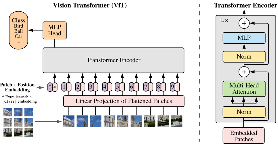
Figure 1: Model overview. We split an image into fixed-size patches, linearly embed each of them, add position embeddings, and feed the resulting sequence of vectors to a standard Transformer encoder. In order to perform classification, we use the standard approach of adding an extra learnable “classification token” to the sequence. The illustration of the Transformer encoder was inspired by Vaswani et al. (2017).
图 1: 模型概览。我们将图像分割为固定大小的图像块 (patch),对每个块进行线性嵌入,添加位置编码,并将得到的向量序列输入标准 Transformer 编码器。为了执行分类任务,我们采用标准方法:在序列中添加一个可学习的"分类标记" (classification token)。Transformer 编码器的示意图灵感来自 Vaswani 等人 (2017) [20]。
3 METHOD
3 方法
In model design we follow the original Transformer (Vaswani et al., 2017) as closely as possible. An advantage of this intentionally simple setup is that scalable NLP Transformer architectures – and their efficient implementations – can be used almost out of the box.
在模型设计上,我们尽可能遵循原版Transformer (Vaswani et al., 2017) 。这种刻意保持简洁的设置有个优势:可扩展的NLP Transformer架构及其高效实现几乎可以直接使用。
3.1 VISION TRANSFORMER (VIT)
3.1 VISION TRANSFORMER (VIT)
An overview of the model is depicted in Figure 1. The standard Transformer receives as input a 1D sequence of token embeddings. To handle 2D images, we reshape the image $\mathbf{x}\in\mathbb{R}^{H\times W\times^{*}C}$ into a sequence of flattened 2D patches $\mathbf{x}_{p}\in\mathbb{R}^{N\times(P^{2}\cdot C)}$ , where $(H,W)$ is the resolution of the original image, $C$ is the number of channels, $(P,P)$ is the resolution of each image patch, and $N=H W/P^{2}$ is the resulting number of patches, which also serves as the effective input sequence length for the Transformer. The Transformer uses constant latent vector size $D$ through all of its layers, so we flatten the patches and map to $D$ dimensions with a trainable linear projection (Eq. 1). We refer to the output of this projection as the patch embeddings.
模型概览如图 1 所示。标准 Transformer 接收一维 token 嵌入序列作为输入。为处理二维图像,我们将图像 $\mathbf{x}\in\mathbb{R}^{H\times W\times^{*}C}$ 重塑为扁平化的二维图像块序列 $\mathbf{x}_{p}\in\mathbb{R}^{N\times(P^{2}\cdot C)}$ ,其中 $(H,W)$ 是原始图像分辨率, $C$ 是通道数, $(P,P)$ 是每个图像块的分辨率, $N=H W/P^{2}$ 是生成的图像块数量,同时也作为 Transformer 的有效输入序列长度。Transformer 在所有层中使用恒定的潜在向量大小 $D$ ,因此我们将图像块展平并通过可训练的线性投影映射到 $D$ 维 (公式 1)。我们将此投影的输出称为图像块嵌入。
Similar to BERT’s [class] token, we prepend a learnable embedding to the sequence of embedded patches $(\mathbf{z}_ {\mathrm{0}}^{\mathrm{0}}=\mathbf{x}_ {\mathrm{class}})$ , whose state at the output of the Transformer encoder $(\mathbf{\bar{z}}_ {L}^{0})$ serves as the image representation y (Eq. 4). Both during pre-training and fine-tuning, a classification head is attached to $\mathbf{z}_{L}^{0}$ . The classification head is implemented by a MLP with one hidden layer at pre-training time and by a single linear layer at fine-tuning time.
类似于BERT的[class] token,我们在嵌入补丁序列前添加一个可学习的嵌入 $(\mathbf{z}_ {\mathrm{0}}^{\mathrm{0}}=\mathbf{x}_ {\mathrm{class}})$ ,其在Transformer编码器输出端的状态 $(\mathbf{\bar{z}}_ {L}^{0})$ 作为图像表示y(公式4)。在预训练和微调阶段,分类头均连接到 $\mathbf{z}_{L}^{0}$ 。该分类头在预训练时由带单隐藏层的MLP实现,微调时则由单个线性层实现。
Position embeddings are added to the patch embeddings to retain positional information. We use standard learnable 1D position embeddings, since we have not observed significant performance gains from using more advanced 2D-aware position embeddings (Appendix D.4). The resulting sequence of embedding vectors serves as input to the encoder.
位置嵌入 (position embeddings) 会添加到块嵌入 (patch embeddings) 中以保留位置信息。我们使用标准的可学习一维位置嵌入,因为我们没有观察到使用更先进的二维感知位置嵌入能带来显著的性能提升 (附录 D.4)。生成的嵌入向量序列将作为编码器的输入。
The Transformer encoder (Vaswani et al., 2017) consists of alternating layers of multi headed selfattention (MSA, see Appendix A) and MLP blocks (Eq. 2, 3). Layernorm (LN) is applied before every block, and residual connections after every block (Wang et al., 2019; Baevski & Auli, 2019).
Transformer编码器 (Vaswani et al., 2017) 由多头自注意力机制 (MSA, 见附录A) 和MLP模块 (公式2、3) 的交替层组成。每个模块前应用层归一化 (LN),每个模块后接残差连接 (Wang et al., 2019; Baevski & Auli, 2019)。
The MLP contains two layers with a GELU non-linearity.
MLP包含两层,带有GELU非线性激活函数。
$$
\begin{array}{r l r l}&{\mathbf{z}_ {0}=[\mathbf{x}_ {\mathrm{class}};\mathbf{x}_ {p}^{1}\mathbf{E};\mathbf{x}_ {p}^{2}\mathbf{E};\cdot\cdot\cdot;\mathbf{x}_ {p}^{N}\mathbf{E}]+\mathbf{E}_ {p o s},}&&{\mathbf{E}\in\mathbb{R}^{(P^{2}\cdot C)\times D},\mathbf{E}_ {p o s}\in\mathbb{R}^{(N+1)\times D}}\ &{\mathbf{z}_ {\ell}^{\prime}\in\mathrm{MSA}(\mathrm{LN}(\mathbf{z}_ {\ell-1}))+\mathbf{z}_ {\ell-1},}&&{\ell=1\dots L}\ &{\mathbf{z}_ {\ell}=\mathrm{MLP}(\mathrm{LN}(\mathbf{z}_ {\ell}^{\prime}))+\mathbf{z}_ {\ell}^{\prime},}&&{\ell=1\dots L}\ &{\mathbf{y}=\mathrm{LN}(\mathbf{z}_{L}^{0})}\end{array}
$$
$$
\begin{array}{r l r l}&{\mathbf{z}_ {0}=[\mathbf{x}_ {\mathrm{class}};\mathbf{x}_ {p}^{1}\mathbf{E};\mathbf{x}_ {p}^{2}\mathbf{E};\cdot\cdot\cdot;\mathbf{x}_ {p}^{N}\mathbf{E}]+\mathbf{E}_ {p o s},}&&{\mathbf{E}\in\mathbb{R}^{(P^{2}\cdot C)\times D},\mathbf{E}_ {p o s}\in\mathbb{R}^{(N+1)\times D}}\ &{\mathbf{z}_ {\ell}^{\prime}\in\mathrm{MSA}(\mathrm{LN}(\mathbf{z}_ {\ell-1}))+\mathbf{z}_ {\ell-1},}&&{\ell=1\dots L}\ &{\mathbf{z}_ {\ell}=\mathrm{MLP}(\mathrm{LN}(\mathbf{z}_ {\ell}^{\prime}))+\mathbf{z}_ {\ell}^{\prime},}&&{\ell=1\dots L}\ &{\mathbf{y}=\mathrm{LN}(\mathbf{z}_{L}^{0})}\end{array}
$$
Inductive bias. We note that Vision Transformer has much less image-specific inductive bias than CNNs. In CNNs, locality, two-dimensional neighborhood structure, and translation e qui variance are baked into each layer throughout the whole model. In ViT, only MLP layers are local and translationally e qui variant, while the self-attention layers are global. The two-dimensional neighborhood structure is used very sparingly: in the beginning of the model by cutting the image into patches and at fine-tuning time for adjusting the position embeddings for images of different resolution (as described below). Other than that, the position embeddings at initialization time carry no information about the 2D positions of the patches and all spatial relations between the patches have to be learned from scratch.
归纳偏置 (Inductive bias)。我们注意到 Vision Transformer 相比 CNN 具有更少的图像特定归纳偏置。在 CNN 中,局部性、二维邻域结构和平移等变性被固化在模型的每一层中。而在 ViT 中,只有 MLP 层具有局部性和平移等变性,而自注意力层是全局的。二维邻域结构的使用非常有限:仅在模型开始时将图像切割成块 (patch),以及在微调时调整不同分辨率图像的位置嵌入 (position embeddings)(如下所述)。除此之外,初始化时的位置嵌入不包含任何关于图像块二维位置的信息,所有块之间的空间关系都必须从头学习。
Hybrid Architecture. As an alternative to raw image patches, the input sequence can be formed from feature maps of a CNN (LeCun et al., 1989). In this hybrid model, the patch embedding projection $\mathbf{E}$ (Eq. 1) is applied to patches extracted from a CNN feature map. As a special case, the patches can have spatial size 1x1, which means that the input sequence is obtained by simply flattening the spatial dimensions of the feature map and projecting to the Transformer dimension. The classification input embedding and position embeddings are added as described above.
混合架构 (Hybrid Architecture)。作为原始图像块的替代方案,输入序列可由CNN (LeCun et al., 1989) 的特征图构成。该混合模型中,块嵌入投影 $\mathbf{E}$ (式1) 作用于从CNN特征图提取的块。特殊情况下,这些块可采用1x1空间尺寸,此时通过简单展平特征图空间维度并投影至Transformer维度即可获得输入序列。分类输入嵌入与位置嵌入按前述方式添加。
3.2 FINE-TUNING AND HIGHER RESOLUTION
3.2 微调与更高分辨率
Typically, we pre-train ViT on large datasets, and fine-tune to (smaller) downstream tasks. For this, we remove the pre-trained prediction head and attach a zero-initialized $D\times K$ feed forward layer, where $K$ is the number of downstream classes. It is often beneficial to fine-tune at higher resolution than pre-training (Touvron et al., 2019; Kolesnikov et al., 2020). When feeding images of higher resolution, we keep the patch size the same, which results in a larger effective sequence length. The Vision Transformer can handle arbitrary sequence lengths (up to memory constraints), however, the pre-trained position embeddings may no longer be meaningful. We therefore perform 2D interpolation of the pre-trained position embeddings, according to their location in the original image. Note that this resolution adjustment and patch extraction are the only points at which an inductive bias about the 2D structure of the images is manually injected into the Vision Transformer.
通常,我们会在大型数据集上对ViT进行预训练,然后针对(较小的)下游任务进行微调。为此,我们会移除预训练的预测头,并附加一个零初始化的$D\times K$前馈层,其中$K$是下游类别数。在比预训练更高分辨率下进行微调通常效果更佳 (Touvron et al., 2019; Kolesnikov et al., 2020)。当输入更高分辨率的图像时,我们保持图像块(patch)大小不变,这会导致有效序列长度增加。Vision Transformer能够处理任意序列长度(受内存限制),但预训练的位置嵌入可能不再有意义。因此,我们会根据预训练位置嵌入在原始图像中的位置进行二维插值。请注意,这种分辨率调整和图像块提取是唯一需要手动将关于图像二维结构的归纳偏置注入Vision Transformer的环节。
4 EXPERIMENTS
4 实验
We evaluate the representation learning capabilities of ResNet, Vision Transformer (ViT), and the hybrid. To understand the data requirements of each model, we pre-train on datasets of varying size and evaluate many benchmark tasks. When considering the computational cost of pre-training the model, ViT performs very favourably, attaining state of the art on most recognition benchmarks at a lower pre-training cost. Lastly, we perform a small experiment using self-supervision, and show that self-supervised ViT holds promise for the future.
我们评估了ResNet、Vision Transformer (ViT) 和混合架构的表征学习能力。为理解各模型的数据需求,我们在不同规模的数据集上进行预训练,并评估多项基准任务。当考虑模型预训练的计算成本时,ViT表现优异,以更低的预训练成本在多数识别基准上达到最优水平。最后,我们进行了小规模自监督实验,结果表明自监督ViT具有未来发展潜力。
4.1 SETUP
4.1 设置
Datasets. To explore model s cal ability, we use the ILSVRC-2012 ImageNet dataset with 1k classes and 1.3M images (we refer to it as ImageNet in what follows), its superset ImageNet-21k with 21k classes and 14M images (Deng et al., 2009), and JFT (Sun et al., 2017) with $18\mathrm{k\Omega}$ classes and 303M high-resolution images. We de-duplicate the pre-training datasets w.r.t. the test sets of the downstream tasks following Kolesnikov et al. (2020). We transfer the models trained on these dataset to several benchmark tasks: ImageNet on the original validation labels and the cleaned-up ReaL labels (Beyer et al., 2020), CIFAR-10/100 (Krizhevsky, 2009), Oxford-IIIT Pets (Parkhi et al., 2012), and Oxford Flowers-102 (Nilsback & Zisserman, 2008). For these datasets, pre-processing follows Kolesnikov et al. (2020).
数据集。为探究模型的可扩展性,我们采用了以下数据集:包含1k类别和130万张图像的ILSVRC-2012 ImageNet数据集(下文简称ImageNet)、其超集ImageNet-21k(含21k类别和1400万张图像)(Deng et al., 2009),以及包含$18\mathrm{k\Omega}$类别和3.03亿张高分辨率图像的JFT数据集(Sun et al., 2017)。我们按照Kolesnikov et al. (2020)的方法对预训练数据集进行下游任务测试集去重处理。将在这些数据集上训练的模型迁移至多个基准任务:原始验证标签和经过清理的ReaL标签(Beyer et al., 2020)的ImageNet、CIFAR-10/100(Krizhevsky, 2009)、Oxford-IIIT Pets(Parkhi et al., 2012)和Oxford Flowers-102(Nilsback & Zisserman, 2008)。这些数据集的预处理流程遵循Kolesnikov et al. (2020)的方案。
Table 1: Details of Vision Transformer model variants.
| Model | Layers | Hidden size D | MLP size | Heads | Params |
| ViT-Base | 12 | 768 | 3072 | 12 | 86M |
| ViT-Large | 24 | 1024 | 4096 | 16 | 307M |
| ViT-Huge | 32 | 1280 | 5120 | 16 | 632M |
表 1: Vision Transformer模型变体详情。
| 模型 | 层数 | 隐藏层大小 D | MLP 大小 | 注意力头数 | 参数量 |
|---|---|---|---|---|---|
| ViT-Base | 12 | 768 | 3072 | 12 | 86M |
| ViT-Large | 24 | 1024 | 4096 | 16 | 307M |
| ViT-Huge | 32 | 1280 | 5120 | 16 | 632M |
We also evaluate on the 19-task VTAB classification suite (Zhai et al., 2019b). VTAB evaluates low-data transfer to diverse tasks, using 1 000 training examples per task. The tasks are divided into three groups: Natural – tasks like the above, Pets, CIFAR, etc. Specialized – medical and satellite imagery, and Structured – tasks that require geometric understanding like localization.
我们还对包含19项任务的VTAB分类套件 (Zhai et al., 2019b) 进行了评估。VTAB通过每项任务使用1000个训练样本,评估低数据量向多样化任务的迁移能力。这些任务分为三组:自然类 (Natural) —— 包含上述宠物分类、CIFAR等类似任务;专业类 (Specialized) —— 涵盖医学和卫星图像;结构化类 (Structured) —— 需要几何理解能力的任务(如定位)。
Model Variants. We base ViT configurations on those used for BERT (Devlin et al., 2019), as summarized in Table 1. The “Base” and “Large” models are directly adopted from BERT and we add the larger “Huge” model. In what follows we use brief notation to indicate the model size and the input patch size: for instance, ViT-L/16 means the “Large” variant with $16\times16$ input patch size. Note that the Transformer’s sequence length is inversely proportional to the square of the patch size, thus models with smaller patch size are computationally more expensive.
模型变体。我们基于BERT (Devlin et al., 2019) 的配置设计了ViT架构,如表1所示。"Base"和"Large"模型直接沿用BERT的设置,并新增了更大的"Huge"模型。后续我们将使用简写表示模型规模和输入图像块(patch)尺寸:例如ViT-L/16表示采用$16\times16$输入块尺寸的"Large"变体。需注意Transformer的序列长度与块尺寸平方成反比,因此较小块尺寸的模型计算开销更大。
For the baseline CNNs, we use ResNet (He et al., 2016), but replace the Batch Normalization layers (Ioffe & Szegedy, 2015) with Group Normalization (Wu & He, 2018), and used standardized convolutions (Qiao et al., 2019). These modifications improve transfer (Kolesnikov et al., 2020), and we denote the modified model “ResNet (BiT)”. For the hybrids, we feed the intermediate feature maps into ViT with patch size of one “pixel”. To experiment with different sequence lengths, we either (i) take the output of stage 4 of a regular ResNet50 or (ii) remove stage 4, place the same number of layers in stage 3 (keeping the total number of layers), and take the output of this extended stage 3. Option (ii) results in a $4\mathbf{x}$ longer sequence length, and a more expensive ViT model.
对于基线CNN,我们采用ResNet (He et al., 2016),但将批量归一化层 (Ioffe & Szegedy, 2015) 替换为组归一化 (Wu & He, 2018),并使用标准化卷积 (Qiao et al., 2019)。这些改进提升了迁移性能 (Kolesnikov et al., 2020),我们将改进后的模型称为"ResNet (BiT)"。在混合架构中,我们将中间特征图输入到补丁尺寸为1个"像素"的ViT中。为测试不同序列长度,我们:(i) 使用常规ResNet50第4阶段的输出,或(ii) 移除第4阶段,在阶段3放置相同数量的层(保持总层数不变),并取扩展后阶段3的输出。方案(ii)会产生$4\mathbf{x}$的序列长度增长,并构建计算成本更高的ViT模型。
Training & Fine-tuning. We train all models, including ResNets, using Adam (Kingma & Ba, 2015) with $\beta_{1}=0.9$ , $\beta_{2}=0.999$ , a batch size of 4096 and apply a high weight decay of 0.1, which we found to be useful for transfer of all models (Appendix D.1 shows that, in contrast to common practices, Adam works slightly better than SGD for ResNets in our setting). We use a linear learning rate warmup and decay, see Appendix B.1 for details. For fine-tuning we use SGD with momentum, batch size 512, for all models, see Appendix B.1.1. For ImageNet results in Table 2, we fine-tuned at higher resolution: 512 for ViT-L/16 and 518 for ViT-H/14, and also used Polyak & Juditsky (1992) averaging with a factor of 0.9999 (Rama chandra n et al., 2019; Wang et al., 2020b).
训练与微调。我们使用Adam (Kingma & Ba, 2015)训练所有模型(包括ResNets),参数设为$\beta_{1}=0.9$、$\beta_{2}=0.999$,批大小为4096,并采用0.1的高权重衰减(附录D.1显示,与常规做法不同,在我们的设置中Adam对ResNets的表现略优于SGD)。学习率采用线性预热与衰减策略,详见附录B.1。微调阶段对所有模型使用带动量的SGD,批大小为512(见附录B.1.1)。表2中的ImageNet结果采用更高分辨率微调:ViT-L/16为512,ViT-H/14为518,并应用Polyak & Juditsky (1992)提出的0.9999系数平均法(Ramachandran et al., 2019; Wang et al., 2020b)。
Metrics. We report results on downstream datasets either through few-shot or fine-tuning accuracy. Fine-tuning accuracies capture the performance of each model after fine-tuning it on the respective dataset. Few-shot accuracies are obtained by solving a regularized least-squares regression problem that maps the (frozen) representation of a subset of training images to ${-1,1}^{K}$ target vectors. This formulation allows us to recover the exact solution in closed form. Though we mainly focus on fine-tuning performance, we sometimes use linear few-shot accuracies for fast on-the-fly evaluation where fine-tuning would be too costly.
指标。我们通过少样本或微调准确率报告下游数据集的结果。微调准确率反映了模型在相应数据集上微调后的性能表现。少样本准确率通过求解一个正则化最小二乘回归问题获得,该问题将(冻结的)训练图像子集表征映射到${-1,1}^{K}$目标向量。这种表述方式使我们能以闭式解的形式获得精确解。虽然我们主要关注微调性能,但在微调成本过高时,也会使用线性少样本准确率进行快速即时评估。
4.2 COMPARISON TO STATE OF THE ART
4.2 与现有技术的对比
We first compare our largest models – ViT-H/14 and ViT-L/16 – to state-of-the-art CNNs from the literature. The first comparison point is Big Transfer (BiT) (Kolesnikov et al., 2020), which performs supervised transfer learning with large ResNets. The second is Noisy Student (Xie et al., 2020), which is a large Efficient Net trained using semi-supervised learning on ImageNet and JFT300M with the labels removed. Currently, Noisy Student is the state of the art on ImageNet and BiT-L on the other datasets reported here. All models were trained on TPUv3 hardware, and we report the number of TPUv3-core-days taken to pre-train each of them, that is, the number of TPU v3 cores (2 per chip) used for training multiplied by the training time in days.
我们首先将最大的模型——ViT-H/14和ViT-L/16——与文献中最先进的CNN进行比较。第一个对比点是Big Transfer (BiT) (Kolesnikov et al., 2020),它使用大型ResNet进行监督迁移学习。第二个是Noisy Student (Xie et al., 2020),这是一个在ImageNet和无标签的JFT300M上通过半监督学习训练的大型Efficient Net。目前,Noisy Student在ImageNet上是最先进的,而BiT-L在本文报告的其他数据集上表现最佳。所有模型均在TPUv3硬件上训练,我们报告了预训练每个模型所消耗的TPUv3-core-days数,即用于训练的TPU v3核心数(每芯片2个)乘以训练天数。
Table 2 shows the results. The smaller ViT-L/16 model pre-trained on JFT-300M outperforms BiT-L (which is pre-trained on the same dataset) on all tasks, while requiring substantially less computational resources to train. The larger model, ViT-H/14, further improves the performance, especially on the more challenging datasets – ImageNet, CIFAR-100, and the VTAB suite. Interestingly, this
表 2 展示了结果。在 JFT-300M 数据集上预训练的较小模型 ViT-L/16 在所有任务上都优于 BiT-L (同样在该数据集上预训练) ,同时训练所需的计算资源显著减少。更大的 ViT-H/14 模型进一步提升了性能,尤其在更具挑战性的数据集上——ImageNet、CIFAR-100 和 VTAB 套件。值得注意的是...
| Ours-JFT (ViT-H/14) | Ours-JFT (ViT-L/16) | Ours-I21k (ViT-L/16) | BiT-L (ResNet152x4) | Noisy Student (EfficientNet-L2) | |
| ImageNet | 88.55±0.04 | 87.76±0.03 | 85.30±0.02 | 87.54± 0.02 | 88.4/88.5 |
| ImageNet ReaL | 90.72±0.05 | 90.54±0.03 | 88.62±0.05 | 90.54 | 90.55 |
| CIFAR-10 | 99.50±0.06 | 99.42±0.03 | 99.15±0.03 | 99.37±0.06 | |
| CIFAR-100 | 94.55±0.04 | 93.90±0.05 | 93.25±0.05 | 93.51±0.08 | |
| Oxford-IlITPets | 97.56±0.03 | 97.32±0.11 | 94.67 ±0.15 | 96.62±0.23 | |
| OxfordFlowers-102 | 99.68±0.02 | 99.74±0.00 | 99.61±0.02 | 99.63±0.03 | |
| VTAB (19 tasks) | 77.63±0.23 | 76.28±0.46 | 72.72±0.21 | 76.29 ±1.70 | 一 |
| TPUv3-core-days | 2.5k | 0.68k | 0.23k | 9.9k | 12.3k |
| Ours-JFT (ViT-H/14) | Ours-JFT (ViT-L/16) | Ours-I21k (ViT-L/16) | BiT-L (ResNet152x4) | Noisy Student (EfficientNet-L2) | |
|---|---|---|---|---|---|
| ImageNet | 88.55±0.04 | 87.76±0.03 | 85.30±0.02 | 87.54±0.02 | 88.4/88.5 |
| ImageNet ReaL | 90.72±0.05 | 90.54±0.03 | 88.62±0.05 | 90.54 | 90.55 |
| CIFAR-10 | 99.50±0.06 | 99.42±0.03 | 99.15±0.03 | 99.37±0.06 | |
| CIFAR-100 | 94.55±0.04 | 93.90±0.05 | 93.25±0.05 | 93.51±0.08 | |
| Oxford-IlITPets | 97.56±0.03 | 97.32±0.11 | 94.67±0.15 | 96.62±0.23 | |
| OxfordFlowers-102 | 99.68±0.02 | 99.74±0.00 | 99.61±0.02 | 99.63±0.03 | |
| VTAB (19 tasks) | 77.63±0.23 | 76.28±0.46 | 72.72±0.21 | 76.29±1.70 | — |
| TPUv3-core-days | 2.5k | 0.68k | 0.23k | 9.9k | 12.3k |
Table 2: Comparison with state of the art on popular image classification benchmarks. We report mean and standard deviation of the accuracies, averaged over three fine-tuning runs. Vision Transformer models pre-trained on the JFT-300M dataset outperform ResNet-based baselines on all datasets, while taking substantially less computational resources to pre-train. ViT pre-trained on the smaller public ImageNet-21k dataset performs well too. ∗Slightly improved $88.5%$ result reported in Touvron et al. (2020).
表 2: 主流图像分类基准的性能对比。我们报告了三次微调运行的平均准确率及其标准差。在 JFT-300M 数据集上预训练的 Vision Transformer 模型在所有数据集上都优于基于 ResNet 的基线模型,同时所需的预训练计算资源显著减少。在较小的公开数据集 ImageNet-21k 上预训练的 ViT 也表现良好。*Touvron 等人 (2020) 报告了略微提升的 $88.5%$ 结果。

Figure 2: Breakdown of VTAB performance in Natural, Specialized, and Structured task groups.
图 2: VTAB在自然(Natural)、专业(Specialized)和结构化(Structured)任务组中的性能分解。
model still took substantially less compute to pre-train than prior state of the art. However, we note that pre-training efficiency may be affected not only by the architecture choice, but also other parameters, such as training schedule, optimizer, weight decay, etc. We provide a controlled study of performance vs. compute for different architectures in Section 4.4. Finally, the ViT-L/16 model pre-trained on the public ImageNet-21k dataset performs well on most datasets too, while taking fewer resources to pre-train: it could be trained using a standard cloud TPUv3 with 8 cores in approximate ly 30 days.
模型的预训练计算量仍远低于此前的最先进水平。但需注意,预训练效率不仅受架构选择影响,还与其他参数相关,如训练计划、优化器、权重衰减等。我们在第4.4节针对不同架构进行了性能与计算资源的对照研究。最后,基于公开ImageNet-21k数据集预训练的ViT-L/16模型在多数数据集上表现优异,且预训练资源消耗更低:使用8核标准云TPUv3约30天即可完成训练。
Figure 2 decomposes the VTAB tasks into their respective groups, and compares to previous SOTA methods on this benchmark: BiT, VIVI – a ResNet co-trained on ImageNet and Youtube (Tschannen et al., 2020), and S4L – supervised plus semi-supervised learning on ImageNet (Zhai et al., 2019a). ViT-H/14 outperforms BiT-R152x4, and other methods, on the Natural and Structured tasks. On the Specialized the performance of the top two models is similar.
图 2: 将VTAB任务分解为各自组别,并与该基准测试中的先前SOTA方法进行比较:BiT、VIVI(在ImageNet和YouTube上联合训练的ResNet)(Tschannen et al., 2020),以及S4L(ImageNet上的监督加半监督学习)(Zhai et al., 2019a)。ViT-H/14在自然和结构化任务上优于BiT-R152x4及其他方法。在专业任务上,前两名模型的性能相近。
4.3 PRE-TRAINING DATA REQUIREMENTS
4.3 预训练数据要求
The Vision Transformer performs well when pre-trained on a large JFT-300M dataset. With fewer inductive biases for vision than ResNets, how crucial is the dataset size? We perform two series of experiments.
视觉Transformer (Vision Transformer) 在大型JFT-300M数据集上预训练时表现优异。相比ResNets,其视觉归纳偏置更少,那么数据集规模有多关键?我们进行了两组实验。
First, we pre-train ViT models on datasets of increasing size: ImageNet, ImageNet-21k, and JFT300M. To boost the performance on the smaller datasets, we optimize three basic regular iz ation parameters – weight decay, dropout, and label smoothing. Figure 3 shows the results after finetuning to ImageNet (results on other datasets are shown in Table 5)2. When pre-trained on the smallest dataset, ImageNet, ViT-Large models under perform compared to ViT-Base models, despite (moderate) regular iz ation. With ImageNet-21k pre-training, their performances are similar. Only with JFT-300M, do we see the full benefit of larger models. Figure 3 also shows the performance region spanned by BiT models of different sizes. The BiT CNNs outperform ViT on ImageNet, but with the larger datasets, ViT overtakes.
首先,我们在逐渐增大的数据集上预训练ViT模型:ImageNet、ImageNet-21k和JFT300M。为了提高在较小数据集上的性能,我们优化了三个基本正则化参数——权重衰减、dropout和标签平滑。图3展示了在ImageNet上微调后的结果(其他数据集的结果见表5)。当在最小的数据集ImageNet上预训练时,尽管进行了(适度)正则化,ViT-Large模型的性能仍低于ViT-Base模型。使用ImageNet-21k预训练时,它们的性能相似。只有在JFT-300M上,我们才能看到更大模型的全部优势。图3还展示了不同尺寸BiT模型的性能范围。BiT CNN在ImageNet上优于ViT,但在更大的数据集上,ViT实现了反超。
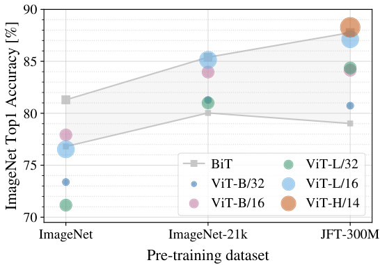
Figure 3: Transfer to ImageNet. While large ViT models perform worse than BiT ResNets (shaded area) when pre-trained on small datasets, they shine when pre-trained on larger datasets. Similarly, larger ViT variants overtake smaller ones as the dataset grows.
图 3: 迁移到 ImageNet。当在小型数据集上进行预训练时,大型 ViT 模型的表现不如 BiT ResNets (阴影区域),但在更大数据集上预训练时表现出色。同样,随着数据集的增大,更大的 ViT 变体会超越较小的变体。
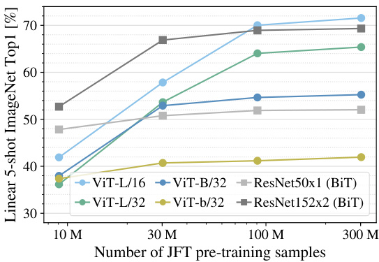
Figure 4: Linear few-shot evaluation on ImageNet versus pre-training size. ResNets perform better with smaller pre-training datasets but plateau sooner than ViT, which performs better with larger pre-training. ViT-b is ViT-B with all hidden dimensions halved.
图 4: ImageNet 上线性少样本评估与预训练规模的关系。ResNet 在较小预训练数据集上表现更好但会更快达到瓶颈,而 ViT 在更大规模预训练时表现更优。ViT-b 指将所有隐藏维度减半的 ViT-B 模型。
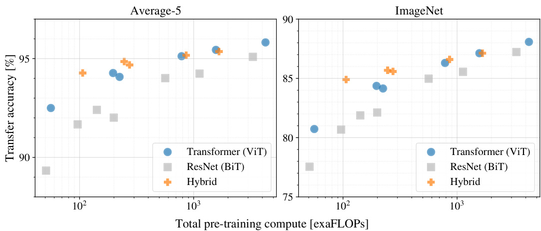
Figure 5: Performance versus pre-training compute for different architectures: Vision Transformers, ResNets, and hybrids. Vision Transformers generally outperform ResNets with the same computational budget. Hybrids improve upon pure Transformers for smaller model sizes, but the gap vanishes for larger models.
图 5: 不同架构的性能与预训练计算量对比:Vision Transformer、ResNet 及混合架构。在相同计算预算下,Vision Transformer 通常优于 ResNet。对于较小模型,混合架构比纯 Transformer 有所提升,但随着模型规模增大,这种差距逐渐消失。
Second, we train our models on random subsets of 9M, 30M, and 90M as well as the full JFT300M dataset. We do not perform additional regular iz ation on the smaller subsets and use the same hyper-parameters for all settings. This way, we assess the intrinsic model properties, and not the effect of regular iz ation. We do, however, use early-stopping, and report the best validation accuracy achieved during training. To save compute, we report few-shot linear accuracy instead of full finetuning accuracy. Figure 4 contains the results. Vision Transformers overfit more than ResNets with comparable computational cost on smaller datasets. For example, ViT-B/32 is slightly faster than ResNet50; it performs much worse on the 9M subset, but better on $90\mathbf{M}+$ subsets. The same is true for Res Net 152 x 2 and ViT-L/16. This result reinforces the intuition that the convolutional inductive bias is useful for smaller datasets, but for larger ones, learning the relevant patterns directly from data is sufficient, even beneficial.
其次,我们在900万、3000万、9000万随机子集以及完整的JFT300M数据集上训练模型。对于较小子集不进行额外正则化处理,所有设置均采用相同超参数。这种方式能评估模型的内在特性,而非正则化效果。不过我们采用了早停策略,并报告训练期间达到的最佳验证准确率。为节省算力,报告的是少样本线性准确率而非完整微调准确率。图4展示了结果:在计算成本相近的情况下,视觉Transformer(ViT)在小数据集上比ResNet更容易过拟合。例如ViT-B/32略快于ResNet50,在900万子集上表现差很多,但在9000万以上子集表现更优。ResNet152x2与ViT-L/16也呈现相同规律。这一结果印证了直觉:卷积归纳偏置对小数据集很有用,但对大数据集而言,直接从数据中学习相关模式不仅足够,甚至更具优势。
Overall, the few-shot results on ImageNet (Figure 4), as well as the low-data results on VTAB (Table 2) seem promising for very low-data transfer. Further analysis of few-shot properties of ViT is an exciting direction of future work.
总体而言,ImageNet上的少样本结果(图 4)和VTAB上的低数据量结果(表 2)在极低数据迁移场景中表现良好。进一步分析ViT的少样本特性是未来工作的一个有趣方向。
4.4 SCALING STUDY
4.4 扩展性研究
We perform a controlled scaling study of different models by evaluating transfer performance from JFT-300M. In this setting data size does not bottleneck the models’ performances, and we assess performance versus pre-training cost of each model. The model set includes: 7 ResNets, R50x1, R50x2 R101x1, $\mathrm{R}152\mathrm{x}1$ , $\mathbf{R}152\mathbf{x}2$ , pre-trained for 7 epochs, plus $\mathbf{R}152\mathbf{x}2$ and ${\tt R}200{\tt X}3$ pre-trained for 14 epochs; 6 Vision Transformers, ViT-B/32, B/16, L/32, L/16, pre-trained for 7 epochs, plus L/16 and H/14 pre-trained for 14 epochs; and 5 hybrids, R50+ViT-B/32, B/16, L/32, L/16 pretrained for 7 epochs, plus $\mathrm{R}50\mathrm{+ViT\mathrm{-L}}/16$ pre-trained for 14 epochs (for hybrids, the number at the end of the model name stands not for the patch size, but for the total dow sampling ratio in the ResNet backbone).
我们通过评估从JFT-300M迁移的性能,对不同模型进行了受控扩展研究。在此设置下,数据规模不会成为模型性能的瓶颈,我们评估了各模型性能与预训练成本的关系。模型集包括:7个ResNet(R50x1、R50x2、R101x1、$\mathrm{R}152\mathrm{x}1$、$\mathbf{R}152\mathbf{x}2$预训练7个周期,外加$\mathbf{R}152\mathbf{x}2$和${\tt R}200{\tt X}3$预训练14个周期);6个Vision Transformer(ViT-B/32、B/16、L/32、L/16预训练7个周期,外加L/16和H/14预训练14个周期);以及5个混合模型(R50+ViT-B/32、B/16、L/32、L/16预训练7个周期,外加$\mathrm{R}50\mathrm{+ViT\mathrm{-L}}/16$预训练14个周期)(对于混合模型,模型名称末尾的数字不代表分块大小,而是ResNet主干中的总降采样率)。
Figure 5 contains the transfer performance versus total pre-training compute (see Appendix D.5 for details on computational costs). Detailed results per model are provided in Table 6 in the Appendix. A few patterns can be observed. First, Vision Transformers dominate ResNets on the performance/compute trade-off. ViT uses approximately $2-4\times$ less compute to attain the same performance (average over 5 datasets). Second, hybrids slightly outperform ViT at small computational budgets, but the difference vanishes for larger models. This result is somewhat surprising, since one might expect convolutional local feature processing to assist ViT at any size. Third, Vision Transformers appear not to saturate within the range tried, motivating future scaling efforts.
图5展示了迁移性能与总预训练计算量的关系(计算成本详情参见附录D.5)。附录中的表6提供了每个模型的详细结果。我们可以观察到几个规律:首先,在性能/计算量权衡方面,Vision Transformer明显优于ResNet。ViT只需消耗约$2-4\times$的计算量即可达到相同性能(5个数据集的平均值)。其次,在较小计算预算时,混合模型略优于ViT,但随着模型规模增大差异逐渐消失。这个结果有些出人意料,因为人们可能认为卷积局部特征处理对各种规模的ViT都有帮助。第三,Vision Transformer在实验规模范围内尚未出现饱和现象,这为未来的扩展研究提供了动力。
4.5 INSPECTING VISION TRANSFORMER
4.5 视觉Transformer (Vision Transformer) 解析
To begin to understand how the Vision Transformer processes image data, we analyze its internal representations. The first layer of the Vision Transformer linearly projects the flattened patches into a lower-dimensional space (Eq. 1). Figure 7 (left) shows the top principal components of the the learned embedding filters. The components resemble plausible basis functions for a low-dimensional representation of the fine structure within each patch.
为了理解Vision Transformer如何处理图像数据,我们分析了其内部表示。Vision Transformer的第一层将展平的图像块线性投影到低维空间(式1)。图7(左)展示了学习到的嵌入过滤器的主要主成分。这些成分类似于每个图像块内部精细结构的低维表示中合理的基函数。
After the projection, a learned position embedding is added to the patch representations. Figure 7 (center) shows that the model learns to encode distance within the image in the similarity of position embeddings, i.e. closer patches tend to have more similar position embeddings. Further, the row-column structure appears; patches in the same row/column have similar embeddings. Finally, a sinusoidal structure is sometimes apparent for larger grids (Appendix D). That the position embeddings learn to represent 2D image topology explains why hand-crafted 2D-aware embedding variants do not yield improvements (Appendix D.4).
投影后,学习得到的位置嵌入会添加到图像块表示中。图7(中)显示,模型学会通过位置嵌入的相似性来编码图像内的距离,即相邻图像块往往具有更相似的位置嵌入。此外,行列结构开始显现:同一行/列的图像块具有相似的嵌入。最后,对于较大网格,有时会出现正弦结构(附录D)。位置嵌入能学习表示二维图像拓扑结构,这解释了为什么手工设计的二维感知嵌入变体未能带来改进(附录D.4)。
Self-attention allows ViT to integrate information across the entire image even in the lowest layers. We investigate to what degree the network makes use of this capability. Specifically, we compute the average distance in image space across which information is integrated, based on the attention weights (Figure 7, right). This “attention distance” is analogous to receptive field size in CNNs.
自注意力机制使ViT即使在最底层也能整合整个图像的信息。我们研究了网络在多大程度上利用了这种能力。具体而言,我们基于注意力权重计算了图像空间中信息整合的平均距离(图7右)。这种"注意力距离"类似于CNN中的感受野大小。
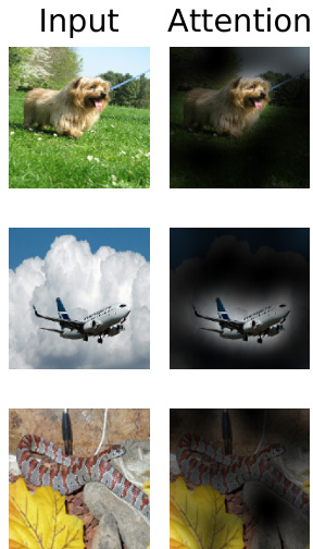
Figure 6: Representative examples of attention from the output token to the input space. See Appendix D.7 for details.
图 6: 输出token对输入空间的注意力代表性示例。详情参见附录 D.7。
We find that some heads attend to most of the image already in the lowest layers, showing that the ability to integrate information globally is indeed used by the model. Other attention heads have consistently small attention distances in the low layers. This highly localized attention is less pronounced in hybrid models that apply a ResNet before the Transformer (Figure 7, right), suggesting that it may serve a similar function as early convolutional layers in CNNs. Further, the attention distance increases with network depth. Globally, we find that the model attends to image regions that are semantically relevant for classification (Figure 6).
我们发现,一些注意力头(attention head)在最底层就已经关注到图像的大部分区域,这表明模型确实具备全局信息整合能力。其他注意力头在低层网络始终保持着较小的注意力距离。这种高度局部化的注意力特性,在采用Transformer前先使用ResNet的混合模型中表现较弱(图7右),暗示其功能可能类似于CNN中的早期卷积层。此外,注意力距离会随着网络深度增加而增大。整体而言,模型关注的图像区域与分类任务具有语义相关性(图6)。
4.6 SELF-SUPERVISION
4.6 自监督学习
Transformers show impressive performance on NLP tasks. However, much of their success stems not only from their excellent s cal ability but also from large scale self-supervised pre-training (Devlin et al., 2019; Radford et al., 2018). We also perform a preliminary exploration on masked patch prediction for self-supervision, mimicking the masked language modeling task used in BERT. With self-supervised pre-training, our smaller ViT-B/16 model achieves $79.9%$ accuracy on ImageNet, a significant improvement of $2%$ to training from scratch, but still $4%$ behind supervised pre-training. Appendix B.1.2 contains further details. We leave exploration of contrastive pre-training (Chen et al., 2020b; He et al., 2020; Bachman et al., 2019; Hénaff et al., 2020) to future work.
Transformer在自然语言处理任务中展现出卓越性能。然而,其成功不仅源于出色的扩展能力,更得益于大规模自监督预训练 (Devlin et al., 2019; Radford et al., 2018)。我们初步探索了掩码补丁预测的自监督方法,模拟BERT中使用的掩码语言建模任务。通过自监督预训练,我们较小的ViT-B/16模型在ImageNet上达到79.9%准确率,相比从头训练显著提升2%,但仍比监督预训练低4%。附录B.1.2包含更多细节。对比预训练 (Chen et al., 2020b; He et al., 2020; Bachman et al., 2019; Hénaff et al., 2020) 的探索将留待未来工作。
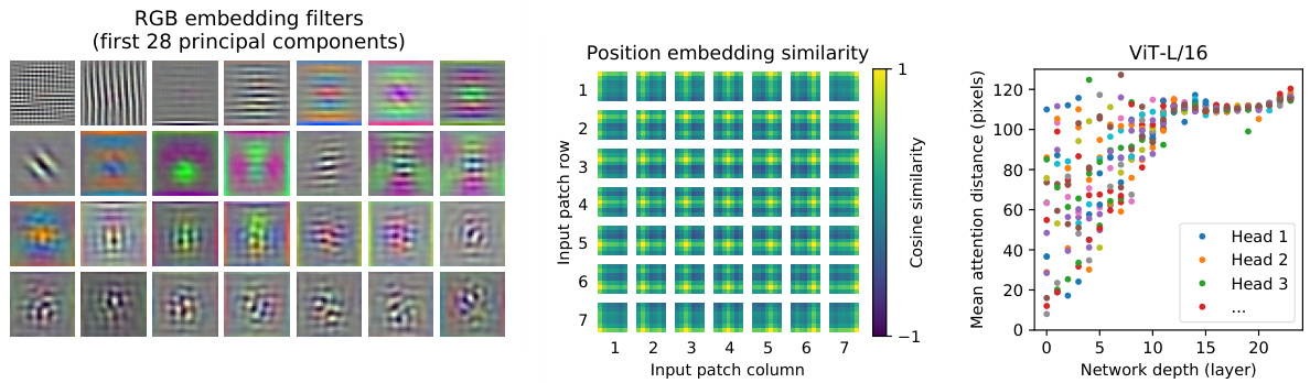
Figure 7: Left: Filters of the initial linear embedding of RGB values of ViT-L/32. Center: Similarity of position embeddings of ViT-L/32. Tiles show the cosine similarity between the position embedding of the patch with the indicated row and column and the position embeddings of all other patches. Right: Size of attended area by head and network depth. Each dot shows the mean attention distance across images for one of 16 heads at one layer. See Appendix D.7 for details.
图 7: 左: ViT-L/32 对 RGB 值初始线性嵌入的滤波器。中: ViT-L/32 位置嵌入的相似性。每个图块显示指定行列的补丁位置嵌入与所有其他补丁位置嵌入之间的余弦相似度。右: 注意力区域大小与网络深度的关系。每个点表示某一层 16 个头在图像上的平均注意力距离。详见附录 D.7。
5 CONCLUSION
5 结论
We have explored the direct application of Transformers to image recognition. Unlike prior works using self-attention in computer vision, we do not introduce image-specific inductive biases into the architecture apart from the initial patch extraction step. Instead, we interpret an image as a sequence of patches and process it by a standard Transformer encoder as used in NLP. This simple, yet scalable, strategy works surprisingly well when coupled with pre-training on large datasets. Thus, Vision Transformer matches or exceeds the state of the art on many image classification datasets, whilst being relatively cheap to pre-train.
我们探索了将Transformer直接应用于图像识别的方法。与之前计算机视觉领域使用自注意力机制的研究不同,除了初始的图像块提取步骤外,我们没有在架构中引入任何针对图像的归纳偏置。相反,我们将图像视为一系列图像块的序列,并使用自然语言处理中标准的Transformer编码器进行处理。这种简单但可扩展的策略,在结合大型数据集预训练时表现出惊人的效果。因此,Vision Transformer在许多图像分类数据集上达到或超越了当前最优水平,同时预训练成本相对较低。
While these initial results are encouraging, many challenges remain. One is to apply ViT to other computer vision tasks, such as detection and segmentation. Our results, coupled with those in Carion et al. (2020), indicate the promise of this approach. Another challenge is to continue exploring selfsupervised pre-training methods. Our initial experiments show improvement from self-supervised pre-training, but there is still large gap between self-supervised and large-scale supervised pretraining. Finally, further scaling of ViT would likely lead to improved performance.
虽然这些初步结果令人鼓舞,但许多挑战仍然存在。其一是将ViT应用于其他计算机视觉任务,如检测和分割。我们的结果与Carion等人 (2020) 的研究共同表明了这种方法的潜力。另一个挑战是继续探索自监督预训练方法。我们的初步实验显示自监督预训练带来了改进,但自监督与大规模监督预训练之间仍存在较大差距。最后,进一步扩展ViT的规模可能会带来性能提升。
ACKNOWLEDGEMENTS
致谢
The work was performed in Berlin, Zurich, and Amsterdam. We thank many colleagues at Google for their help, in particular Andreas Steiner for crucial help with the infrastructure and the opensource release of the code; Joan Puigcerver and Maxim Neumann for help with the large-scale training infrastructure; Dmitry Lepikhin, Aravindh Mahendran, Daniel Keysers, Mario Lucic, Noam Shazeer, Ashish Vaswani, and Colin Raffel for useful discussions.
工作在柏林、苏黎世和阿姆斯特丹进行。我们感谢谷歌众多同事的帮助,特别是Andreas Steiner在基础设施和代码开源发布方面的关键支持;Joan Puigcerver和Maxim Neumann在大规模训练基础设施上的协助;以及Dmitry Lepikhin、Aravindh Mahendran、Daniel Keysers、Mario Lucic、Noam Shazeer、Ashish Vaswani和Colin Raffel的有益讨论。
REFERENCES
参考文献
Samira Abnar and Willem Zuidema. Quantifying attention flow in transformers. In ACL, 2020.
Samira Abnar 和 Willem Zuidema. 量化Transformer中的注意力流. 载于ACL, 2020.
Philip Bachman, R Devon Hjelm, and William Buchwalter. Learning representations by maximizing mutual information across views. In NeurIPS, 2019.
Philip Bachman、R Devon Hjelm 和 William Buchwalter。通过跨视图最大化互信息学习表征。收录于 NeurIPS,2019年。
ICML, 2020.
ICML,2020。
Sergey Ioffe and Christian Szegedy. Batch normalization: Accelerating deep network training by reducing internal covariate shift. 2015.
Sergey Ioffe 和 Christian Szegedy. 批量归一化 (Batch Normalization): 通过减少内部协变量偏移加速深度网络训练. 2015.
CVPR, 2020.
CVPR,2020。
Table 3: Hyper parameters for training. All models are trained with a batch size of 4096 and learning rate warmup of $10\mathrm{k\Omega}$ steps. For ImageNet we found it beneficial to additionally apply gradient clipping at global norm 1. Training resolution is 224.
| Models | Dataset | Epochs | Base LR | LR decay | Weight decay | Dropout |
| ViT-B/{16,32} | JFT-300M | 7 | 8·10-4 | linear | 0.1 | 0.0 |
| ViT-L/32 | JFT-300M | 7 | 6·10-4 | linear | 0.1 | 0.0 |
| ViT-L/16 | JFT-300M | 7/14 | 4·10-4 | linear | 0.1 | 0.0 |
| ViT-H/14 | JFT-300M | 14 | 3·10-4 | linear | 0.1 | 0.0 |
| R50x{1,2} | JFT-300M | 7 | 10-3 | linear | 0.1 | 0.0 |
| R101x1 | JFT-300M | 7 | 8·10-4 | linear | 0.1 | 0.0 |
| R152x{1,2} | JFT-300M | 7 | 6·10-4 | linear | 0.1 | 0.0 |
| R50+ViT-B/{16,32} | JFT-300M | 7 | 8·10-4 | linear | 0.1 | 0.0 |
| R50+ViT-L/32 | JFT-300M | 7 | 2·10-4 | linear | 0.1 | 0.0 |
| R50+ViT-L/16 | JFT-300M | 7/14 | 4·10-4 | linear | 0.1 | 0.0 |
| ViT-B/{16,32} | ImageNet-21k | 90 | 10-3 | linear | 0.03 | 0.1 |
| ViT-L/{16,32} | ImageNet-21k | 30/90 | 10-3 | linear | 0.03 | 0.1 |
| ViT-* | ImageNet | 300 | 3·10-3 | cosine | 0.3 | 0.1 |
表 3: 训练超参数。所有模型均以4096的批量大小和 $10\mathrm{k\Omega}$ 步数的学习率预热进行训练。对于ImageNet数据集,我们发现额外应用全局范数为1的梯度裁剪效果更佳。训练分辨率为224。
| 模型 | 数据集 | 训练轮数 | 基础学习率 | 学习率衰减 | 权重衰减 | Dropout |
|---|---|---|---|---|---|---|
| ViT-B/{16,32} | JFT-300M | 7 | 8·10-4 | linear | 0.1 | 0.0 |
| ViT-L/32 | JFT-300M | 7 | 6·10-4 | linear | 0.1 | 0.0 |
| ViT-L/16 | JFT-300M | 7/14 | 4·10-4 | linear | 0.1 | 0.0 |
| ViT-H/14 | JFT-300M | 14 | 3·10-4 | linear | 0.1 | 0.0 |
| R50x{1,2} | JFT-300M | 7 | 10-3 | linear | 0.1 | 0.0 |
| R101x1 | JFT-300M | 7 | 8·10-4 | linear | 0.1 | 0.0 |
| R152x{1,2} | JFT-300M | 7 | 6·10-4 | linear | 0.1 | 0.0 |
| R50+ViT-B/{16,32} | JFT-300M | 7 | 8·10-4 | linear | 0.1 | 0.0 |
| R50+ViT-L/32 | JFT-300M | 7 | 2·10-4 | linear | 0.1 | 0.0 |
| R50+ViT-L/16 | JFT-300M | 7/14 | 4·10-4 | linear | 0.1 | 0.0 |
| ViT-B/{16,32} | ImageNet-21k | 90 | 10-3 | linear | 0.03 | 0.1 |
| ViT-L/{16,32} | ImageNet-21k | 30/90 | 10-3 | linear | 0.03 | 0.1 |
| ViT-* | ImageNet | 300 | 3·10-3 | cosine | 0.3 | 0.1 |
APPENDIX
附录
A MULTIHEAD SELF-ATTENTION
多头自注意力机制
Standard qkv self-attention (SA, Vaswani et al. (2017)) is a popular building block for neural architectures. For each element in an input sequence $\mathbf{z}\in\dot{\mathbb{R}}^{N\times\dot{D}}$ , we compute a weighted sum over all values $\mathbf{v}$ in the sequence. The attention weights $A_{i j}$ are based on the pairwise similarity between two elements of the sequence and their respective query $\mathbf{q}^{i}$ and key ${\bf k}^{j}$ representations.
标准qkv自注意力机制 (SA, Vaswani et al. (2017) [20]) 是神经架构中的常用模块。对于输入序列 $\mathbf{z}\in\dot{\mathbb{R}}^{N\times\dot{D}}$ 中的每个元素,我们计算序列中所有值 $\mathbf{v}$ 的加权和。注意力权重 $A_{i j}$ 基于序列中两个元素之间的成对相似度及其各自的查询 $\mathbf{q}^{i}$ 和键 ${\bf k}^{j}$ 表示。
$$
\begin{array}{r l}&{[{\bf q},{\bf k},{\bf v}]={\bf z}{\bf U}_ {q k v}\qquad{\bf U}_ {q k v}\in\mathbb{R}^{D\times3D_{h}},}\ &{A=\mathrm{softmax}\left({\bf q}{\bf k}^{\top}/\sqrt{D_{h}}\right)\qquad\quad A\in\mathbb{R}^{N\times N},}\ &{\qquad\mathrm{SA}({\bf z})=A{\bf v}.}\end{array}
$$
$$
\begin{array}{r l}&{[{\bf q},{\bf k},{\bf v}]={\bf z}{\bf U}_ {q k v}\qquad{\bf U}_ {q k v}\in\mathbb{R}^{D\times3D_{h}},}\ &{A=\mathrm{softmax}\left({\bf q}{\bf k}^{\top}/\sqrt{D_{h}}\right)\qquad\quad A\in\mathbb{R}^{N\times N},}\ &{\qquad\mathrm{SA}({\bf z})=A{\bf v}.}\end{array}
$$
Multihead self-attention (MSA) is an extension of SA in which we run $k$ self-attention operations, called “heads”, in parallel, and project their concatenated outputs. To keep compute and number of parameters constant when changing $k$ , $D_{h}$ (Eq. 5) is typically set to $D/k$ .
多头自注意力 (Multihead Self-Attention, MSA) 是自注意力 (SA) 的扩展形式,通过并行运行 $k$ 个称为"头"的自注意力操作,并对它们的拼接输出进行投影。为确保在调整 $k$ 时计算量和参数量保持不变,通常将 $D_{h}$ (公式5) 设为 $D/k$。
$$
\mathrm{MSA}(\mathbf{z})=[\mathrm{SA}_ {1}(z);\mathrm{SA}_ {2}(z);\cdots,\mathrm{SA}_ {k}(z)]\mathbf{U}_ {m s a}\qquad\mathbf{U}_ {m s a}\in\mathbb{R}^{k\cdot D_{h}\times D}
$$
$$
\mathrm{MSA}(\mathbf{z})=[\mathrm{SA}_ {1}(z);\mathrm{SA}_ {2}(z);\cdots,\mathrm{SA}_ {k}(z)]\mathbf{U}_ {m s a}\qquad\mathbf{U}_ {m s a}\in\mathbb{R}^{k\cdot D_{h}\times D}
$$
B EXPERIMENT DETAILS
B 实验细节
B.1 TRAINING
B.1 训练
Table 3 summarizes our training setups for our different models. We found strong regular iz ation to be key when training models from scratch on ImageNet. Dropout, when used, is applied after every dense layer except for the the qkv-projections and directly after adding positional- to patch embeddings. Hybrid models are trained with the exact setup as their ViT counterparts. Finally, all training is done on resolution 224.
表 3 总结了不同模型的训练设置。我们发现,在 ImageNet 上从头训练模型时,强正则化 (regularization) 是关键。使用 Dropout 时,除 qkv 投影层外,每个密集层后都会应用 Dropout,并在添加位置嵌入 (positional embedding) 到块嵌入 (patch embedding) 后直接应用。混合模型采用与 ViT 对应模型完全相同的设置进行训练。最后,所有训练均在 224 分辨率下完成。
B.1.1 FINE-TUNING
B.1.1 微调
We fine-tune all ViT models using SGD with a momentum of 0.9. We run a small grid search over learning rates, see learning rate ranges in Table 4. To do so, we use small sub-splits from the training set ( $10%$ for Pets and Flowers, $2%$ for CIFAR, $1%$ ImageNet) as development set and train on the remaining data. For final results we train on the entire training set and evaluate on the respective test data. For fine-tuning ResNets and hybrid models we use the exact same setup, with the only exception of ImageNet where we add another value 0.06 to the learning rate sweep. Additionally,
我们使用动量为0.9的SGD对所有ViT模型进行微调。我们在学习率范围内进行了小规模网格搜索,具体范围见表4。为此,我们从训练集中划分出小型子集(Pets和Flowers数据集取10%,CIFAR取2%,ImageNet取1%)作为开发集,并在剩余数据上进行训练。最终结果是在完整训练集上训练后,在对应测试数据上评估得出。对于ResNets和混合模型的微调,除ImageNet数据集额外增加0.06的学习率扫描值外,其余设置完全相同。
| Dataset | Steps | Base LR |
| ImageNet | 20000 | {0.003,0.01,0.03,0.06} |
| CIFAR100 | 10000 | {0.001,0.003,0.01,0.03} |
| CIFAR10 | 10000 | 0.001,0.003,0.01,0.03} |
| Oxford-IlITPets | 500 | 0.001,0.003,0.01,0.03} |
| OxfordFlowers-102 | 500 | {0.001,0.003,0.01,0.03} |
| VTAB(19 tasks) | 2500 | 0.01 |
| 数据集 | 步数 | 基础学习率 |
|---|---|---|
| ImageNet | 20000 | {0.003,0.01,0.03,0.06} |
| CIFAR100 | 10000 | {0.001,0.003,0.01,0.03} |
| CIFAR10 | 10000 | 0.001,0.003,0.01,0.03} |
| Oxford-IIITPets | 500 | 0.001,0.003,0.01,0.03} |
| OxfordFlowers-102 | 500 | {0.001,0.003,0.01,0.03} |
| VTAB(19 tasks) | 2500 | 0.01 |
Table 4: Hyper parameters for fine-tuning. All models are fine-tuned with cosine learning rate decay, a batch size of 512, no weight decay, and grad clipping at global norm 1. If not mentioned otherwise, fine-tuning resolution is 384.
表 4: 微调超参数。所有模型均采用余弦学习率衰减进行微调,批次大小为512,无权重衰减,梯度裁剪全局范数为1。除非另有说明,微调分辨率均为384。
for ResNets we also run the setup of Kolesnikov et al. (2020) and select the best results across this run and our sweep. Finally, if not mentioned otherwise, all fine-tuning experiments run at 384 resolution (running fine-tuning at different resolution than training is common practice (Kolesnikov et al., 2020)).
对于ResNet,我们还运行了Kolesnikov等人 (2020) 的实验设置,并从中选取最佳结果。最后,除非另有说明,所有微调实验均在384分辨率下进行(训练与微调采用不同分辨率是常见做法 (Kolesnikov et al., 2020))。
When transferring ViT models to another dataset, we remove the whole head (two linear layers) and replace it by a single, zero-initialized linear layer outputting the number of classes required by the target dataset. We found this to be a little more robust than simply re-initializing the very last layer.
在将ViT模型迁移到另一个数据集时,我们会移除整个头部(两个线性层),并将其替换为一个零初始化的单线性层,该层的输出数量与目标数据集所需的类别数相匹配。我们发现这种方法比简单地重新初始化最后一层要更稳健一些。
For VTAB we follow the protocol in Kolesnikov et al. (2020), and use the same hyper parameter setting for all tasks. We use a learning rate of 0.01 and train for 2500 steps (Tab. 4). We chose this setting by running a small sweep over two learning rates and two schedules, and selecting the setting with the highest VTAB score on the 200-example validation sets. We follow the pre-processing used in Kolesnikov et al. (2020), except that we do not use task-specific input resolutions. Instead we find that Vision Transformer benefits most from a high resolution $(384\times384)$ for all tasks.
对于VTAB,我们遵循Kolesnikov等人 (2020) 的协议,并对所有任务使用相同的超参数设置。我们采用0.01的学习率并训练2500步 (表4)。该设置是通过对两种学习率和两种调度方案进行小范围扫描,并选择在200样本验证集上获得最高VTAB分数的配置而确定的。我们沿用了Kolesnikov等人 (2020) 的预处理方法,但未使用任务特定的输入分辨率。相反,我们发现Vision Transformer在所有任务中都能从高分辨率 $(384\times384)$ 获得最佳效果。
B.1.2 SELF-SUPERVISION
B.1.2 自监督学习
We employ the masked patch prediction objective for preliminary self-supervision experiments. To do so we corrupt $50%$ of patch embeddings by either replacing their embeddings with a learnable [mask] embedding $(80%)$ , a random other patch embedding $(10%)$ or just keeping them as is $(10%)$ . This setup is very similar to the one used for language by Devlin et al. (2019). Finally, we predict the 3-bit, mean color (i.e., 512 colors in total) of every corrupted patch using their respective patch representations.
我们采用掩码补丁预测目标进行初步自监督实验。具体做法是:对50%的补丁嵌入进行破坏处理,其中80%替换为可学习的[mask]嵌入,10%替换为随机其他补丁嵌入,剩余10%保持原样。该设置与Devlin等人(2019)在语言领域采用的方法高度相似。最后,我们利用各补丁的表征来预测每个被破坏补丁的3位均值颜色(即总计512种颜色)。
We trained our self-supervised model for 1M steps (ca. 14 epochs) with batch size 4096 on JFT. We use Adam, with a base learning rate of $2\cdot10^{-4}$ , warmup of $10\mathrm{k\Omega}$ steps and cosine learning rate decay. As prediction targets for pre training we tried the following settings: 1) predicting only the mean, 3bit color (i.e., 1 prediction of 512 colors), 2) predicting a $4\times4$ downsized version of the $16\times16$ patch with 3bit colors in parallel (i.e., 16 predictions of 512 colors), 3) regression on the full patch using L2 (i.e., 256 regressions on the 3 RGB channels). Surprisingly, we found that all worked quite well, though L2 was slightly worse. We report final results only for option 1) because it has shown best few-shot performance. We also experimented with $15%$ corruption rate as used by Devlin et al. (2019) but results were also slightly worse on our few-shot metrics.
我们在JFT数据集上以4096的批量大小训练了自监督模型100万步(约14个周期)。采用Adam优化器,基础学习率为$2\cdot10^{-4}$,经过$10\mathrm{k\Omega}$步的热身后采用余弦学习率衰减。预训练阶段尝试了以下预测目标设置:1) 仅预测均值,3位色深(即对512种颜色做1次预测);2) 并行预测$16\times16$图像块经$4\times4$下采样后的3位色深版本(即对512种颜色做16次预测);3) 使用L2损失对完整图像块进行回归(即对RGB三通道进行256次回归)。出乎意料的是,三种方案效果均较好,但L2略逊。由于方案1在少样本指标上表现最优,我们仅报告该方案的最终结果。我们还尝试了Devlin等人(2019)采用的15%数据损坏率,但在少样本评估指标上效果也稍差。
Lastly, we would like to remark that our instantiation of masked patch prediction doesn’t require such an enormous amount of pre training nor a large dataset such as JFT in order to lead to similar performance gains on ImageNet classification. That is, we observed diminishing returns on downstream performance after $100\mathrm{k\Omega}$ pre training steps, and see similar gains when pre training on ImageNet.
最后需要说明的是,我们采用的掩码图像块预测方法无需海量预训练数据(如JFT数据集)或超长训练周期,就能在ImageNet分类任务上实现相近的性能提升。具体而言,我们发现当下游性能在预训练步数达到$100\mathrm{k\Omega}$后会出现收益递减现象,且仅使用ImageNet进行预训练也能获得类似效果。
C ADDITIONAL RESULTS
C 附加结果
We report detailed results corresponding to the figures presented in the paper. Table 5 corresponds to Figure 3 from the paper and shows transfer performance of different ViT models pre-trained on datasets of increasing size: ImageNet, ImageNet-21k, and JFT-300M. Table 6 corresponds to
我们报告了与论文中图表相对应的详细结果。表5对应论文中的图3,展示了在不同规模数据集(ImageNet、ImageNet-21k和JFT-300M)上预训练的ViT模型迁移性能。表6对应
Table 5: Top1 accuracy (in $%$ ) of Vision Transformer on various datasets when pre-trained on ImageNet, ImageNet-21k or JFT300M. These values correspond to Figure 3 in the main text. Models are fine-tuned at 384 resolution. Note that the ImageNet results are computed without additional techniques (Polyak averaging and 512 resolution images) used to achieve results in Table 2.
| ViT-B/16 | ViT-B/32 | ViT-L/16 | ViT-L/32 | ViT-H/14 | ||
| ImageNet | CIFAR-10 | 98.13 | 97.77 | 97.86 | 97.94 | |
| CIFAR-100 | 87.13 | 86.31 | 86.35 | 87.07 | ||
| ImageNet | 77.91 | 73.38 | 76.53 | 71.16 | ||
| ImageNet ReaL | 83.57 | 79.56 | 82.19 | 77.83 | ||
| Oxford Flowers-102 | 89.49 | 85.43 | 89.66 | 86.36 | ||
| Oxford-IIIT-Pets | 93.81 | 92.04 | 93.64 | 91.35 | ||
| ImageNet-21k | CIFAR-10 | 98.95 | 98.79 | 99.16 | 99.13 | 99.27 |
| CIFAR-100 | 91.67 | 91.97 | 93.44 | 93.04 | 93.82 | |
| ImageNet | 83.97 | 81.28 | 85.15 | 80.99 | 85.13 | |
| ImageNet ReaL | 88.35 | 86.63 | 88.40 | 85.65 | 88.70 | |
| Oxford Flowers-102 Oxford-IIIT-Pets | 99.38 | 99.11 | 99.61 | 99.19 | 99.51 | |
| 94.43 | 93.02 | 94.73 | 93.09 | 94.82 | ||
| JFT-300M | CIFAR-10 | 99.00 | 98.61 | 99.38 | 99.19 | 99.50 |
| CIFAR-100 | 91.87 | 90.49 | 94.04 | 92.52 | 94.55 | |
| ImageNet | 84.15 | 80.73 | 87.12 | 84.37 | 88.04 | |
| ImageNet ReaL | 88.85 | 86.27 | 89.99 | 88.28 | 90.33 | |
| Oxford Flowers-102 | 99.56 | 99.27 | 99.56 | 99.45 | 99.68 | |
| Oxford-IIIT-Pets | 95.80 | 93.40 | 97.11 | 95.83 | 97.56 | |
表 5: Vision Transformer 在 ImageNet、ImageNet-21k 或 JFT300M 预训练后在各数据集上的 Top1 准确率 (单位: $%$ )。这些数值对应正文中的图 3。模型均在 384 分辨率下微调。请注意,ImageNet 结果未使用表 2 中采用的额外技术 (Polyak 平均和 512 分辨率图像) 进行计算。
| ViT-B/16 | ViT-B/32 | ViT-L/16 | ViT-L/32 | ViT-H/14 | ||
|---|---|---|---|---|---|---|
| ImageNet | CIFAR-10 | 98.13 | 97.77 | 97.86 | 97.94 | |
| CIFAR-100 | 87.13 | 86.31 | 86.35 | 87.07 | ||
| ImageNet | 77.91 | 73.38 | 76.53 | 71.16 | ||
| ImageNet ReaL | 83.57 | 79.56 | 82.19 | 77.83 | ||
| Oxford Flowers-102 | 89.49 | 85.43 | 89.66 | 86.36 | ||
| Oxford-IIIT-Pets | 93.81 | 92.04 | 93.64 | 91.35 | ||
| ImageNet-21k | CIFAR-10 | 98.95 | 98.79 | 99.16 | 99.13 | 99.27 |
| CIFAR-100 | 91.67 | 91.97 | 93.44 | 93.04 | 93.82 | |
| ImageNet | 83.97 | 81.28 | 85.15 | 80.99 | 85.13 | |
| ImageNet ReaL | 88.35 | 86.63 | 88.40 | 85.65 | 88.70 | |
| Oxford Flowers-102 | 99.38 | 99.11 | 99.61 | 99.19 | 99.51 | |
| Oxford-IIIT-Pets | 94.43 | 93.02 | 94.73 | 93.09 | 94.82 | |
| JFT-300M | CIFAR-10 | 99.00 | 98.61 | 99.38 | 99.19 | 99.50 |
| CIFAR-100 | 91.87 | 90.49 | 94.04 | 92.52 | 94.55 | |
| ImageNet | 84.15 | 80.73 | 87.12 | 84.37 | 88.04 | |
| ImageNet ReaL | 88.85 | 86.27 | 89.99 | 88.28 | 90.33 | |
| Oxford Flowers-102 | 99.56 | 99.27 | 99.56 | 99.45 | 99.68 | |
| Oxford-IIIT-Pets | 95.80 | 93.40 | 97.11 | 95.83 | 97.56 |
| name | Epochs | ImageNet | ImageNetReaL | CIFAR-10 | CIFAR-100 | Pets | Flowers | exaFLOPs |
| ViT-B/32 | 7 | 80.73 | 86.27 | 98.61 | 90.49 | 93.40 | 99.27 | 55 |
| ViT-B/16 | 7 | 84.15 | 88.85 | 99.00 | 91.87 | 95.80 | 99.56 | 224 |
| ViT-L/32 | 7 | 84.37 | 88.28 | 99.19 | 92.52 | 95.83 | 99.45 | 196 |
| ViT-L/16 | 7 | 86.30 | 89.43 | 99.38 | 93.46 | 96.81 | 99.66 | 783 |
| ViT-L/16 | 14 | 87.12 | 89.99 | 99.38 | 94.04 | 97.11 | 99.56 | 1567 |
| ViT-H/14 | 14 | 88.08 | 90.36 | 99.50 | 94.71 | 97.11 | 99.71 | 4262 |
| ResNet50x1 | 7 | 77.54 | 84.56 | 97.67 | 86.07 | 91.11 | 94.26 | 50 |
| ResNet50x2 | 7 | 82.12 | 87.94 | 98.29 | 89.20 | 93.43 | 97.02 | 199 |
| ResNet101xl | 7 | 80.67 | 87.07 | 98.48 | 89.17 | 94.08 | 95.95 | 96 |
| ResNet152x1 | 7 | 81.88 | 87.96 | 98.82 | 90.22 | 94.17 | 96.94 | 141 |
| ResNet152x2 | 7 | 84.97 | 89.69 | 99.06 | 92.05 | 95.37 | 98.62 | 563 |
| ResNet152x2 | 14 | 85.56 | 89.89 | 99.24 | 91.92 | 95.75 | 98.75 | 1126 |
| ResNet200x3 | 14 | 87.22 | 90.15 | 99.34 | 93.53 | 96.32 | 99.04 | 3306 |
| R50x1+ViT-B/32 | 7 | 84.90 | 89.15 | 99.01 | 92.24 | 95.75 | 99.46 | 106 |
| R50x1+ViT-B/16 | 7 | 85.58 | 89.65 | 99.14 | 92.63 | 96.65 | 99.40 | 274 |
| R50x1+ViT-L/32 | 7 | 85.68 | 89.04 | 99.24 | 92.93 | 96.97 | 99.43 | 246 |
| R50x1+ViT-L/16 | 7 | 86.60 | 89.72 | 99.18 | 93.64 | 97.03 | 99.40 | 859 |
| R50x1+ViT-L/16 | 14 | 87.12 | 89.76 | 99.31 | 93.89 | 97.36 | 99.11 | 1668 |
| name | Epochs | ImageNet | ImageNetReaL | CIFAR-10 | CIFAR-100 | Pets | Flowers | exaFLOPs |
|---|---|---|---|---|---|---|---|---|
| ViT-B/32 | 7 | 80.73 | 86.27 | 98.61 | 90.49 | 93.40 | 99.27 | 55 |
| ViT-B/16 | 7 | 84.15 | 88.85 | 99.00 | 91.87 | 95.80 | 99.56 | 224 |
| ViT-L/32 | 7 | 84.37 | 88.28 | 99.19 | 92.52 | 95.83 | 99.45 | 196 |
| ViT-L/16 | 7 | 86.30 | 89.43 | 99.38 | 93.46 | 96.81 | 99.66 | 783 |
| ViT-L/16 | 14 | 87.12 | 89.99 | 99.38 | 94.04 | 97.11 | 99.56 | 1567 |
| ViT-H/14 | 14 | 88.08 | 90.36 | 99.50 | 94.71 | 97.11 | 99.71 | 4262 |
| ResNet50x1 | 7 | 77.54 | 84.56 | 97.67 | 86.07 | 91.11 | 94.26 | 50 |
| ResNet50x2 | 7 | 82.12 | 87.94 | 98.29 | 89.20 | 93.43 | 97.02 | 199 |
| ResNet101xl | 7 | 80.67 | 87.07 | 98.48 | 89.17 | 94.08 | 95.95 | 96 |
| ResNet152x1 | 7 | 81.88 | 87.96 | 98.82 | 90.22 | 94.17 | 96.94 | 141 |
| ResNet152x2 | 7 | 84.97 | 89.69 | 99.06 | 92.05 | 95.37 | 98.62 | 563 |
| ResNet152x2 | 14 | 85.56 | 89.89 | 99.24 | 91.92 | 95.75 | 98.75 | 1126 |
| ResNet200x3 | 14 | 87.22 | 90.15 | 99.34 | 93.53 | 96.32 | 99.04 | 3306 |
| R50x1+ViT-B/32 | 7 | 84.90 | 89.15 | 99.01 | 92.24 | 95.75 | 99.46 | 106 |
| R50x1+ViT-B/16 | 7 | 85.58 | 89.65 | 99.14 | 92.63 | 96.65 | 99.40 | 274 |
| R50x1+ViT-L/32 | 7 | 85.68 | 89.04 | 99.24 | 92.93 | 96.97 | 99.43 | 246 |
| R50x1+ViT-L/16 | 7 | 86.60 | 89.72 | 99.18 | 93.64 | 97.03 | 99.40 | 859 |
| R50x1+ViT-L/16 | 14 | 87.12 | 89.76 | 99.31 | 93.89 | 97.36 | 99.11 | 1668 |
Table 6: Detailed results of model scaling experiments. These correspond to Figure 5 in the main paper. We show transfer accuracy on several datasets, as well as the pre-training compute (in exaFLOPs).
表 6: 模型缩放实验的详细结果。这些结果对应主论文中的图 5。我们展示了在多个数据集上的迁移准确率,以及预训练计算量 (单位: exaFLOPs)。
Figure 5 from the paper and shows the transfer performance of ViT, ResNet, and hybrid models of varying size, as well as the estimated computational cost of their pre-training.
图 5: 论文中的图表,展示了不同规模的 ViT、ResNet 以及混合模型的迁移性能,以及它们预训练的计算成本估计。
D ADDITIONAL ANALYSES
D 补充分析
D.1 SGD VS. ADAM FOR RESNETS
D.1 ResNet中的SGD与Adam优化器对比
ResNets are typically trained with SGD and our use of Adam as optimizer is quite unconventional. Here we show the experiments that motivated this choice. Namely, we compare the fine-tuning performance of two ResNets – 50x1 and $152\mathbf{x}2$ – pre-trained on JFT with SGD and Adam. For SGD, we use the hyper parameters recommended by Kolesnikov et al. (2020). Results are presented in Table 7. Adam pre-training outperforms SGD pre-training on most datasets and on average. This justifies the choice of Adam as the optimizer used to pre-train ResNets on JFT. Note that the absolute numbers are lower than those reported by Kolesnikov et al. (2020), since we pre-train only for 7 epochs, not 30.
ResNet通常使用SGD进行训练,而我们采用Adam作为优化器的做法相当非传统。此处展示促使我们做出该选择的实验:比较两个在JFT数据集上分别用SGD和Adam预训练的ResNet(50x1和$152\mathbf{x}2$)的微调性能。对于SGD,我们采用Kolesnikov等人 (2020) 推荐的超参数。结果如表7所示。在大多数数据集及平均表现上,Adam预训练都优于SGD预训练,这证实了选择Adam作为JFT上预训练ResNet优化器的合理性。需注意绝对数值低于Kolesnikov等人 (2020) 报告的结果,因为我们仅进行7轮预训练而非30轮。
Table 7: Fine-tuning ResNet models pre-trained with Adam and SGD.
| ResNet50 | ResNet152x2 | |||
| Dataset | Adam | SGD | Adam | SGD |
| ImageNet | 77.54 | 78.24 | 84.97 | 84.37 |
| CIFAR10 | 97.67 | 97.46 | 99.06 | 99.07 |
| CIFAR100 | 86.07 | 85.17 | 92.05 | 91.06 |
| Oxford-mITPets | 91.11 | 91.00 | 95.37 | 94.79 |
| OxfordFlowers-102 | 94.26 | 92.06 | 98.62 | 99.32 |
| Average | 89.33 | 88.79 | 94.01 | 93.72 |
表 7: 使用Adam和SGD预训练的ResNet模型微调结果
| ResNet50 | ResNet152x2 | |
|---|---|---|
| 数据集 | Adam | SGD |
| ImageNet | 77.54 | 78.24 |
| CIFAR10 | 97.67 | 97.46 |
| CIFAR100 | 86.07 | 85.17 |
| Oxford-mITPets | 91.11 | 91.00 |
| OxfordFlowers-102 | 94.26 | 92.06 |
| 平均 | 89.33 | 88.79 |

Figure 8: Scaling different model dimensions of the Vision Transformer.
图 8: Vision Transformer不同模型维度的扩展效果
D.2 TRANSFORMER SHAPE
D.2 Transformer 架构
We ran ablations on scaling different dimensions of the Transformer architecture to find out which are best suited for scaling to very large models. Figure 8 shows 5-shot performance on ImageNet for different configurations. All configurations are based on a ViT model with 8 layers, $D=1024$ , $D_{M L P}=2048$ and a patch size of 32, the intersection of all lines. We can see that scaling the depth results in the biggest improvements which are clearly visible up until 64 layers. However, diminishing returns are already visible after 16 layers. Interestingly, scaling the width of the network seems to result in the smallest changes. Decreasing the patch size and thus increasing the effective sequence length shows surprisingly robust improvements without introducing parameters. These findings suggest that compute might be a better predictor of performance than the number of parameters, and that scaling should emphasize depth over width if any. Overall, we find that scaling all dimensions proportionally results in robust improvements.
我们对Transformer架构的不同维度进行缩放消融实验,以确定哪些维度最适合扩展到超大规模模型。图8展示了不同配置在ImageNet上的5样本性能。所有配置均基于8层ViT模型,其中$D=1024$、$D_{MLP}=2048$、图像块尺寸为32(所有曲线的交点)。实验表明:深度缩放带来的性能提升最为显著,这种增益在64层之前保持明显,但超过16层后已出现收益递减现象;有趣的是,网络宽度缩放产生的变化最小;而减小图像块尺寸(从而增加有效序列长度)能在不引入额外参数的情况下带来显著且稳定的性能提升。这些发现表明:计算量可能比参数量更能预测模型性能,且缩放策略应优先考虑深度而非宽度。总体而言,我们发现按比例缩放所有维度能获得稳健的性能提升。
D.3 HEAD TYPE AND CLASS TOKEN
D.3 头部类型与类别Token
In order to stay as close as possible to the original Transformer model, we made use of an additional [class] token, which is taken as image representation. The output of this token is then transformed into a class prediction via a small multi-layer perceptron (MLP) with tanh as non-linearity in the single hidden layer.
为了尽可能贴近原始Transformer模型,我们额外使用了一个[class] token作为图像表征。该token的输出随后通过一个小型多层感知机(MLP)转化为类别预测,其中单隐藏层采用tanh作为非线性激活函数。
This design is inherited from the Transformer model for text, and we use it throughout the main paper. An initial attempt at using only image-patch embeddings, globally average-pooling (GAP) them, followed by a linear classifier—just like ResNet’s final feature map—performed very poorly. However, we found that this is neither due to the extra token, nor to the GAP operation. Instead,
该设计沿用了文本Transformer模型的架构,并在论文主体部分全程采用。我们最初尝试仅使用图像块嵌入 (image-patch embeddings) ,通过全局平均池化 (GAP) 处理后接线性分类器(类似ResNet最终特征图的做法),但效果极差。研究发现,问题既非由额外token引起,也非GAP操作所致,而是...

Figure 9: Comparison of class-token and global average pooling class if i ers. Both work similarly well, but require different learning-rates.
图 9: 类别token与全局平均池化分类器的对比。两者表现相近,但需要不同的学习率。
| Pos. Emb. | Default/Stem | Every Layer | Every Layer-Shared |
| NoPos.Emb. | 0.61382 | N/A | N/A |
| 1-DPos.Emb. | 0.64206 | 0.63964 | 0.64292 |
| 2-DPos.Emb. | 0.64001 | 0.64046 | 0.64022 |
| Rel. Pos. Emb. | 0.64032 | N/A | N/A |
| 位置编码 (Pos. Emb.) | 默认/主干 (Default/Stem) | 逐层 (Every Layer) | 逐层共享 (Every Layer-Shared) |
|---|---|---|---|
| 无位置编码 (NoPos.Emb.) | 0.61382 | N/A | N/A |
| 一维位置编码 (1-DPos.Emb.) | 0.64206 | 0.63964 | 0.64292 |
| 二维位置编码 (2-DPos.Emb.) | 0.64001 | 0.64046 | 0.64022 |
| 相对位置编码 (Rel. Pos. Emb.) | 0.64032 | N/A | N/A |
Table 8: Results of the ablation study on positional embeddings with ViT-B/16 model evaluated on ImageNet 5-shot linear.
表 8: 基于ViT-B/16模型在ImageNet 5-shot linear评估的位置嵌入消融研究结果
the difference in performance is fully explained by the requirement for a different learning-rate, see Figure 9.
性能差异完全由不同学习率需求所致,见图 9:
D.4 POSITIONAL EMBEDDING
D.4 位置嵌入 (Positional Embedding)
We ran ablations on different ways of encoding spatial information using positional embedding. We tried the following cases:
我们对使用位置嵌入编码空间信息的不同方法进行了消融实验。尝试了以下情况:
In addition to different ways of encoding spatial information, we also tried different ways of incorpora ting this information in our model. For the 1-dimensional and 2-dimensional positional embeddings, we tried three different cases: (1) add positional embeddings to the inputs right after the stem of them model and before feeding the inputs to the Transformer encoder (default across all other experiments in this paper); (2) learn and add positional embeddings to the inputs at the beginning of each layer; (3) add a learned positional embeddings to the inputs at the beginning of each layer (shared between layers).
除了不同的空间信息编码方式外,我们还尝试了在模型中融入这些信息的不同方法。对于一维和二维位置嵌入(positional embeddings),我们尝试了三种不同方案:(1) 在模型主干网络后、输入Transformer编码器前添加位置嵌入(本文其他实验的默认设置);(2) 在每层开始时学习并添加位置嵌入;(3) 在每层开始时添加共享的可学习位置嵌入。

Figure 10: Position embeddings of models trained with different hyper parameters.
图 10: 采用不同超参数训练的模型位置嵌入效果。
Table 8 summarizes the results from this ablation study on a ViT-B/16 model. As we can see, while there is a large gap between the performances of the model with no positional embedding and models with positional embedding, there is little to no difference between different ways of encoding positional information. We speculate that since our Transformer encoder operates on patch-level inputs, as opposed to pixel-level, the differences in how to encode spatial information is less important. More precisely, in patch-level inputs, the spatial dimensions are much smaller than the original pixel-level inputs, e.g., $14\times14$ as opposed to $224\times224$ , and learning to represent the spatial relations in this resolution is equally easy for these different positional encoding strategies. Even so, the specific pattern of position embedding similarity learned by the network depends on the training hyper parameters (Figure 10).
表 8 总结了在 ViT-B/16 模型上进行的消融研究结果。可以看出,虽然无位置嵌入模型与带位置嵌入模型之间存在较大性能差距,但不同位置信息编码方式之间几乎没有差异。我们推测,由于 Transformer 编码器处理的是图像块(patch)级输入而非像素级输入,空间信息编码方式的差异影响较小。具体而言,在图像块级输入中,空间维度远小于原始像素级输入(例如 $14\times14$ 对比 $224\times224$ ),在此分辨率下学习空间关系表示对这些不同位置编码策略而言难度相当。即便如此,网络学习到的位置嵌入相似性具体模式仍取决于训练超参数(图 10)。

Figure 11: Size of attended area by head and network depth. Attention distance was computed for 128 example images by averaging the distance between the query pixel and all other pixels, weighted by the attention weight. Each dot shows the mean attention distance across images for one of 16 heads at one layer. Image width is 224 pixels.
图 11: 各注意力头及网络深度的关注区域大小。通过对128张样本图像计算查询像素与所有其他像素的加权平均距离(权重为注意力权重)得出注意力距离。每个点表示某一层中16个注意力头在图像上的平均注意力距离。图像宽度为224像素。
D.5 EMPIRICAL COMPUTATIONAL COSTS
D.5 实证计算成本
We are also interested in real-world speed of the architectures on our hardware, which is not always well predicted by theoretical FLOPs due to details like lane widths and cache sizes. For this purpose, we perform timing of inference speed for the main models of interest, on a TPUv3 accelerator; the difference between inference and backprop speed is a constant model-independent factor.
我们还关注这些架构在实际硬件上的运行速度,由于通道宽度和缓存大小等细节因素,理论FLOPs并不能准确预测实际性能。为此,我们在TPUv3加速器上对主要目标模型进行了推理速度计时;推理与反向传播速度之间的差异是一个与模型无关的恒定系数。
Figure 12 (left) shows how many images one core can handle per second, across various input sizes. Every single point refers to the peak performance measured across a wide range of batch-sizes. As can be seen, the theoretical bi-quadratic scaling of ViT with image size only barely starts happening for the largest models at the largest resolutions.
图 12 (左) 展示了单个核心在不同输入尺寸下每秒能处理的图像数量。每个数据点均代表在多种批量大小下测得的峰值性能。如图所示,ViT (Vision Transformer) 理论上的双二次缩放特性仅在最大分辨率下的最大模型中才开始略微显现。
Another quantity of interest is the largest batch-size each model can fit onto a core, larger being better for scaling to large datasets. Figure 12 (right) shows this quantity for the same set of models. This shows that large ViT models have a clear advantage in terms of memory-efficiency over ResNet models.
另一个关注的指标是每个模型能适配到单个核心的最大批次大小,该数值越大意味着越能高效扩展到大型数据集。图12(右)展示了同组模型的对比数据,表明大型ViT模型在内存效率方面较ResNet模型具有明显优势。

Figure 12: Left: Real wall-clock timings of various architectures across input sizes. ViT models have speed comparable to similar ResNets. Right: Largest per-core batch-size fitting on device with various architectures across input sizes. ViT models are clearly more memory-efficient.
图 12: 左: 不同架构在不同输入规模下的实际耗时对比。ViT模型速度与同类ResNet相当。右: 不同架构在不同输入规模下单个计算核心可容纳的最大批次大小。ViT模型明显更具内存效率。
D.6 AXIAL ATTENTION
D.6 轴向注意力
Axial Attention (Huang et al., 2020; Ho et al., 2019) is a simple, yet effective technique to run selfattention on large inputs that are organized as multidimensional tensors. The general idea of axial attention is to perform multiple attention operations, each along a single axis of the input tensor, instead of applying 1-dimensional attention to the flattened version of the input. In axial attention, each attention mixes information along a particular axis, while keeping information along the other axes independent. Along this line, Wang et al. (2020b) proposed the Axial Res Net model in which all the convolutions with kernel size $3\times3$ in a ResNet50 are replaced by axial self-attention, i.e. a row and column attention, augmented by relative positional encoding. We have implemented Axial Res Net as a baseline model.3.
轴向注意力 (Axial Attention) (Huang et al., 2020; Ho et al., 2019) 是一种简单而有效的技术,用于对组织为多维张量的大规模输入进行自注意力计算。其核心思想是沿输入张量的单个轴执行多次注意力操作,而非对展平后的输入进行一维注意力计算。在轴向注意力中,每次注意力操作仅混合特定轴上的信息,同时保持其他轴上的信息相互独立。基于这一思路,Wang et al. (2020b) 提出了轴向残差网络 (Axial ResNet) 模型,该模型将 ResNet50 中所有 $3\times3$ 核大小的卷积替换为轴向自注意力 (即行注意力和列注意力),并通过相对位置编码进行增强。我们已将轴向残差网络实现为基线模型。
Moreover, we have modified ViT to process inputs in the 2-dimensional shape, instead of a 1- dimensional sequence of patches, and incorporate Axial Transformer blocks, in which instead of a self-attention followed by an MLP, we have a a row-self-attention plus an MLP followed by a column-self-attention plus an MLP.
此外,我们对ViT进行了修改,使其能够处理二维形状的输入,而非一维的补丁序列,并引入了轴向Transformer模块。在这些模块中,我们不再采用自注意力机制后接MLP的结构,而是采用行自注意力加MLP,再接列自注意力加MLP的方式。
Figure 13, present the performance of Axial ResNet, Axial-ViT-B/32 and Axial-ViT-B/16 on ImageNet 5shot linear, when pretrained on JFT dataset, verses the pre training compute, both in terms of number of FLOPs and inference time (example per seconds). As we can see, both Axial-ViT-B/32 and Axial-ViT-B/16 do better than their ViT-B counterpart in terms of performance, but it comes at the cost of more compute. This is because in Axial-ViT models, each Transformer block with global self-attention is replaced by two Axial Transformer blocks, one with row and one with column selfattention and although the sequence length that self-attention operates on is smaller in axial case, there is a extra MLP per Axial-ViT block. For the Axial Res Net, although it looks reasonable in terms of accuracy/compute trade-off (Figure 13, left), the naive implementation is extremely slow on TPUs (Figure 13, right).
图 13: 展示了在 JFT 数据集上预训练的 Axial ResNet、Axial-ViT-B/32 和 Axial-ViT-B/16 在 ImageNet 5-shot linear 任务中的性能表现,对比了预训练计算量(以 FLOPs 和每秒推理样本数为单位)。可以看出,Axial-ViT-B/32 和 Axial-ViT-B/16 在性能上都优于对应的 ViT-B 模型,但代价是更高的计算量。这是因为在 Axial-ViT 模型中,每个具有全局自注意力 (self-attention) 的 Transformer 块被替换为两个轴向 Transformer 块(分别包含行自注意力和列自注意力),尽管轴向模型的自注意力操作序列长度更短,但每个 Axial-ViT 块额外增加了一个 MLP。对于 Axial ResNet,虽然在准确率/计算量权衡方面表现合理(图 13 左),但其原生实现在 TPU 上的运行速度极慢(图 13 右)。

Figure 13: Performance of Axial-Attention based models, in terms of top-1 accuracy on ImageNet 5-shot linear, versus their speed in terms of number of FLOPs (left) and inference time (left).
图 13: 基于轴向注意力(Axial-Attention)模型的性能表现,展示其在ImageNet 5-shot线性评估中的top-1准确率,以及以FLOPs数量(左)和推理时间(左)衡量的速度对比。
D.7 ATTENTION DISTANCE
D.7 注意力距离
To understand how ViT uses self-attention to integrate information across the image, we analyzed the average distance spanned by attention weights at different layers (Figure 11). This “attention distance” is analogous to receptive field size in CNNs. Average attention distance is highly variable across heads in lower layers, with some heads attending to much of the image, while others attend to small regions at or near the query location. As depth increases, attention distance increases for all heads. In the second half of the network, most heads attend widely across tokens.
为了理解ViT如何利用自注意力机制整合图像信息,我们分析了不同层级注意力权重的平均跨越距离(图11)。这种"注意力距离"类似于CNN中的感受野大小。在底层网络中,不同注意力头的平均距离差异显著:部分注意力头关注图像大部分区域,而另一些则聚焦于查询位置附近的小范围区域。随着网络深度增加,所有注意力头的关注范围逐渐扩大。在网络后半部分,多数注意力头能够广泛关注各个token。
D.8 ATTENTION MAPS
D.8 注意力图
To compute maps of the attention from the output token to the input space (Figures 6 and 14), we used Attention Rollout (Abnar & Zuidema, 2020). Briefly, we averaged attention weights of ViTL/16 across all heads and then recursively multiplied the weight matrices of all layers. This accounts for the mixing of attention across tokens through all layers.
为了计算从输出token到输入空间的注意力分布图(图6和图14),我们采用了注意力展开法(Abnar & Zuidema, 2020)。具体而言,我们先对ViTL/16所有注意力头的权重进行平均,然后递归地乘以所有层的权重矩阵。这种方法能够反映注意力在所有层之间通过token的混合情况。
D.9 OBJECTNET RESULTS
D.9 OBJECTNET 结果
We also evaluate our flagship ViT-H/14 model on the ObjectNet benchmark following the evaluation setup in Kolesnikov et al. (2020), resulting in $82.1%$ top-5 accuracy and $61.7%$ top-1 accuracy.
我们还按照 Kolesnikov 等人 (2020) 的评估设置,在 ObjectNet 基准上评估了我们的旗舰 ViT-H/14 模型,获得了 82.1% 的 top-5 准确率和 61.7% 的 top-1 准确率。
D.10 VTAB BREAKDOWN
D.10 VTAB 细分
Table 9 shows the scores attained on each of the VTAB-1k tasks.
表 9: 展示了在VTAB-1k各项任务上获得的分数。

Figure 14: Further example attention maps as in Figure 6 (random selection).
图 14: 与图 6 类似的更多注意力图示例(随机选取)。
Table 9: Breakdown of VTAB-1k performance across tasks.
| Caltech101 | CIFAR-100 | TD D | Flowers102 | Pets | Sun397 | SVHN | Camelyon | EuroSAT | Resisc45 | Retinopathy | Clevr-Count | Clevr-Dist | dSpr-Loc DMLab | dSpr-Ori | KITTI-Dist | sNORB-Azim | sNORB-Elev | Mean | ||
| ViT-H/14 (JFT) | 95.3 | 85.5 | 75.2 | 99.7 | 97.2 | 65.0 | 88.9 | 83.3 | 96.7 91.4 | 76.6 | 91.7 | 63.853.1 | 79.46 63.3 | 84.5 | 533.251.2 | 77.6 | ||||
| ViT-L/16 (JFT) | 95.4 | 81.9 | 74.3 | 99.79 | 96.7 | 63.5 | 87.4 | 83.6 | 596.5 | 89.7 | 77.1 | 86.4 | :63.1 | 49.7 | 74.5 | 60.5 | 82.2 | 36.2 | 51.1 | 76.3 |
| ViT-L/16 (I21k) | 90.8 | 84.1 | 74.1 | 99.39 | 92.7 | 61.0 | 80.9 | 82.5 | 95.6 | 85.2 | 75.3 | 70.3 56.1 | 41.9 | 74.7 | 64.9 | 79.930.5 | 41.7 | 72.7 |
表 9: VTAB-1k 任务性能分解
| Caltech101 | CIFAR-100 | TD D | Flowers102 | Pets | Sun397 | SVHN | Camelyon | EuroSAT | Resisc45 | Retinopathy | Clevr-Count | Clevr-Dist | dSpr-Loc DMLab | dSpr-Ori | KITTI-Dist | sNORB-Azim | sNORB-Elev | Mean | ||
|---|---|---|---|---|---|---|---|---|---|---|---|---|---|---|---|---|---|---|---|---|
| ViT-H/14 (JFT) | 95.3 | 85.5 | 75.2 | 99.7 | 97.2 | 65.0 | 88.9 | 83.3 | 96.7 91.4 | 76.6 | 91.7 | 63.853.1 | 79.46 63.3 | 84.5 | 533.251.2 | 77.6 | ||||
| ViT-L/16 (JFT) | 95.4 | 81.9 | 74.3 | 99.79 | 96.7 | 63.5 | 87.4 | 83.6 | 596.5 | 89.7 | 77.1 | 86.4 | :63.1 | 49.7 | 74.5 | 60.5 | 82.2 | 36.2 | 51.1 | 76.3 |
| ViT-L/16 (I21k) | 90.8 | 84.1 | 74.1 | 99.39 | 92.7 | 61.0 | 80.9 | 82.5 | 95.6 | 85.2 | 75.3 | 70.3 56.1 | 41.9 | 74.7 | 64.9 | 79.930.5 | 41.7 | 72.7 |