Semantic 2 Graph: 基于图的多模态特征融合视频动作分割方法

Abstract

摘要

Video action segmentation have been widely applied in many fields. Most previous studies employed video-based vision models for this purpose. However, they often rely on a large receptive field, LSTM or Transformer methods to capture long-term dependencies within videos, leading to significant computational resource requirements. To address this challenge, graph-based model was proposed. However, previous graph-based models are less accurate. Hence, this study introduces a graph-structured approach named Semantic 2 Graph, to model long-term dependencies in videos, thereby reducing computational costs and raise the accuracy. We construct a graph structure of video at the frame-level. Temporal edges are utilized to model the temporal relations and action order within videos. Additionally, we have designed positive and negative semantic edges, accompanied by corresponding edge weights, to capture both long-term and short-term semantic relationships in video actions. Node attributes encompass a rich set of multi-modal features extracted from video content, graph structures, and label text, encompassing visual, structural, and semantic cues. To synthesize this multi-modal information effectively, we employ a graph neural network (GNN) model to fuse multi-modal features for node action label classification. Experimental results demonstrate that Semantic 2 Graph outperforms state-of-the-art methods in terms of performance, particularly on benchmark datasets such as GTEA and 50Salads. Multiple ablation experiments further validate the effectiveness of semantic features in enhancing model performance. Notably, the inclusion of semantic edges in Semantic 2 Graph allows for the cost-effective capture of long-term dependencies, affirming its utility in addressing the challenges posed by computational resource constraints in video-based vision models.

视频动作分割已广泛应用于多个领域。多数先前研究采用基于视频的视觉模型实现这一目标。但这些方法通常依赖大感受野、LSTM或Transformer方法来捕捉视频中的长时依赖关系，导致计算资源需求显著。为应对这一挑战，基于图的模型被提出。然而，现有基于图的模型精度较低。为此，本研究提出名为Semantic 2 Graph的图结构方法，通过建模视频中的长时依赖关系来降低计算成本并提升精度。我们在帧级别构建视频图结构：使用时序边建模视频中的时序关系与动作顺序；同时设计带权值的正负语义边，以捕捉视频动作的长短期语义关联。节点属性包含从视频内容、图结构和标签文本中提取的多模态特征，涵盖视觉、结构和语义线索。为有效融合多模态信息，我们采用图神经网络(GNN)模型进行节点动作标签分类的多模态特征融合。实验结果表明，Semantic 2 Graph在GTEA和50Salads等基准数据集上性能优于现有最优方法。多项消融实验进一步验证了语义特征对模型性能的提升作用。值得注意的是，Semantic 2 Graph通过引入语义边实现了长时依赖关系的低成本捕捉，有效解决了基于视频的视觉模型面临的算力约束难题。

Keywords: Video action segmentation, graph neural networks, computer vision, semantic features, multi-modal fusion

关键词：视频动作分割、图神经网络、计算机视觉、语义特征、多模态融合

1 Introduction

1 引言

Video action segmentation stands as a pivotal technology extensively employed across diverse applications and has attracted a great deal of study interest in recent years. Owing to the fruitful progress of deep learning in computer vision tasks, early methods utilize video-based vision models for video action segmentation [1]. In video-based vision models, video is viewed as a sequence of RGB frames [2]. The video-based vision models frequently rely on expanding sliding windows (receptive fields) [1, 3], increasing network depth, introducing attention mechanisms, stacking modules, LSTM or Transformer methods to extract spatio-temporal varying local and global features from videos to represent complex relations in videos [3, 4]. However, these dependency modeling approaches, while effective, comes at a substantial computational cost [1].

视频动作分割是一项广泛应用于多种场景的关键技术，近年来引发了大量研究兴趣。得益于深度学习在计算机视觉任务中的显著进展，早期方法采用基于视频的视觉模型进行视频动作分割[1]。这类模型将视频视为连续的RGB帧序列[2]，通常通过扩展滑动窗口（感受野）[1,3]、增加网络深度、引入注意力机制、堆叠模块、LSTM或Transformer等方法，从视频中提取时空变化的局部与全局特征，以表征视频中的复杂关系[3,4]。然而这些依赖建模方法虽然有效，却伴随着高昂的计算成本[1]。

With the advances in Graph Neural Networks (GNNs), numerous graph models have been implemented for video action segmentation and recognition over the last few years [1, 3, 5, 6]. Most video-based graph models are skeleton-based, which extract skeleton graphs from video frames relying on human pose information instead of RGB pixel data [2, 7-9]. A video is represented as a sequence of skeleton graphs. However, skeleton-based method degrades visual features and is only appropriate for specific scenes with skeleton information. Consequently, several studies [1, 3, 6, 10] transform a video (or video clip) into a graph in which each node represents a video frame (or video clip). These methods are graph-based in this paper. For example, Hamza Khan et al. [5] uses graph convolutional network to learn the visual features of frames and the relationship between neighbor frames for timestampsupervised action segmentation. Dong Wang et al. [6] proposed Dilated Temporal Graph Reasoning Module (DTGRM) to construct a multi-layer detailed temporal graph of the video to capture and model the temporal relationships and dependencies in the video. They construct S-Graph (Similarity Graph) and LGraph (Learned Graph) for each frame. The attribute of each node is frame-wise feature that extracted by I3D. Graph-based methods have larger receptive fields and lower costs to capture long-term dependencies [1, 3, 6], and are also able to capture non-sequential temporal relations. Thus, most graph-based models can address the computationally expensive problem of visual models capturing long-term dependencies in videos. In recent years, many works [1, 2, 9, 11-13] have demonstrated that multi-modal features substantially improve the accuracy of results [9, 14]. However, compared to vision models, existing graph-based methods are less accurate. Because they only utilize the visual features of frames as node attributes and ignore other modal features (such as label text), which results in suboptimal results. Therefore, multi-modal features are adopted to facilitate video reasoning, especially for natural language supervised information [1, 4, 15, 16] in this paper. Hence, the motivation of this study is to design a graph-based model with higher accuracy.

随着图神经网络 (GNN) 的发展，过去几年已有大量图模型被应用于视频动作分割与识别任务 [1, 3, 5, 6]。大多数基于视频的图模型采用骨骼架构，这类方法依赖人体姿态信息而非RGB像素数据从视频帧中提取骨骼图 [2, 7-9]。视频被表示为骨骼图序列。但基于骨骼的方法会弱化视觉特征，且仅适用于具有骨骼信息的特定场景。因此，多项研究 [1, 3, 6, 10] 将视频（或视频片段）转化为图结构，其中每个节点代表一个视频帧（或视频片段）。本文将这些方法归类为基于图的方法。例如，Hamza Khan 等人 [5] 使用图卷积网络学习帧的视觉特征及相邻帧间关系，用于时间戳监督的动作分割。Dong Wang 等人 [6] 提出扩张时序图推理模块 (DTGRM)，通过构建视频的多层精细时序图来捕捉和建模视频中的时序关系与依赖。他们为每帧构建相似图 (S-Graph) 和学习图 (L-Graph)，节点属性由I3D提取的逐帧特征构成。基于图的方法具有更大的感受野和更低的计算成本来捕捉长期依赖 [1, 3, 6]，还能捕获非顺序的时序关系。因此，多数基于图的模型能解决视觉模型捕捉视频长期依赖时计算量大的问题。近年来，许多研究 [1, 2, 9, 11-13] 证明多模态特征能显著提升结果准确性 [9, 14]。但与视觉模型相比，现有基于图的方法精度较低，因其仅使用帧的视觉特征作为节点属性，忽略了其他模态特征（如标签文本），导致次优结果。为此，本文采用多模态特征（特别是自然语言监督信息 [1, 4, 15, 16]）来增强视频推理。因此，本研究旨在设计具有更高精度的基于图的模型。

Our approach is to leverage the powerful relational modeling of graphs to reduce computational and multi-modal feature fusion further improves graph model performance. The graphstructured representation of video provides valuable information about the temporal relation between different frames or video segments. The graph structure can capture both temporal coherence and action order, which allows us to model the sequential nature of actions in videos. Hence, in this paper, we introduce a graph-based method named Semantic 2 Graph, to turn the video action segmentation into node classification. The explicit goal of Semantic 2 Graph is to reduce the computational demands associated with video-based vision models. To this end, we construct a graph structure of video at the frame-level. Adding temporal edges, semantic edges, and self-loop edges to capture both long-term and short-term relations in the video frame sequences. Moreover, node attributes encompass a rich set of multi-modal features, include visual, structural, and semantic cues. Structural features provide important action order information. The incorporation of structural features enables our approach to model the dynamic evolution of actions over time and helps to accurately segment actions and recognize boundaries. Semantic features provide a higher-level understanding of actions occurring in videos. Furthermore, semantic features can assist in handling challenging scenarios, such as ambiguous or rare actions, by providing additional cues for disambiguation. Node neighborhood information is reflected through structural features. Notably, semantic features are the text embedding of sentences encoded by a visual language pre-trained model [4, 15, 16], and the sentence is label-text extended using prompt-based method [4, 15, 16]. A GNNs model, that is a spatial-based graph convolutional neural network (GCN) model suitable for processing directed graphs [17, 18], is employed for multi-modal feature fusion to predict node action labels. Experimental results demonstrate that our approach outperforms state-of-the-art methods in terms of performance. Our contributions are summarized as follows:

我们的方法利用图结构强大的关系建模能力来降低计算量，而多模态特征融合进一步提升了图模型性能。视频的图结构表征能提供不同帧或视频片段间时序关系的宝贵信息。这种图结构既能捕捉时序连贯性，又能反映动作顺序，使我们能够建模视频中动作的序列特性。为此，本文提出名为Semantic 2 Graph的图方法，将视频动作分割转化为节点分类任务。该方法的显式目标是降低视频视觉模型的计算需求。我们构建了帧级视频图结构，通过添加时序边、语义边和自循环边来捕捉视频帧序列中的长短期关系。节点属性包含视觉、结构和语义线索组成的多模态特征集：结构特征提供关键动作顺序信息，能建模动作的动态演化过程，助力精准动作分割与边界识别；语义特征通过视觉语言预训练模型[4,15,16]编码的标签文本扩展句子的文本嵌入，提供对视频动作的高层理解，可处理模糊或罕见动作等复杂场景。节点邻域信息通过结构特征体现。我们采用适合处理有向图的空间图卷积网络(GCN)[17,18]进行多模态特征融合以预测节点动作标签。实验表明本方法性能优于现有技术，主要贡献包括：

● We present a small-scale and flexible graph model for video action segmentation. We describe a method for constructing the graph of videos and design three kinds of edges to model finegrained relations in videos. Especially, the semantic edges reduce the cost of capturing long-term temporal relations. We introduce multi-modal features combining visual, structural, and semantic features as node attributes. In particular, the semantic features of textual prompt-based are more effective than only label words for enhance semantic content.

● 我们提出了一种用于视频动作分割的小规模灵活图模型。我们描述了构建视频图的方法，并设计了三种边来建模视频中的细粒度关系。特别是，语义边降低了捕捉长期时序关系的成本。我们引入了结合视觉、结构和语义特征的多模态特征作为节点属性。其中，基于文本提示的语义特征比仅使用标签词更能有效增强语义内容。

In the following sections, we will elaborate on the details of our graph-based approach and present empirical evidence of its efficacy. In the next section, we first introduce how we construct the graph model.

在接下来的章节中，我们将详细阐述基于图(graph)的方法细节，并提供其有效性的实证依据。下一节首先介绍图模型的构建方式。

2 Our approach

2 我们的方法

This work aims to address the challenges of video action segmentation and recognition utilizing graph models. To do this, we present a graph-based method named Semantic 2 Graph.

本研究旨在利用图模型解决视频动作分割与识别的挑战。为此，我们提出了一种基于图的方法，称为Semantic 2 Graph。

2.1 Notation

2.1 符号表示

Let $\mathbf{V}={\nu_{I},...,\nu_{N}}$ denote the set of untrimmed videos. The $i\cdot$ - th video $\nu_{i}={f_{t}\in\mathbb{R}^{\mathrm{H}\times\mathsf{W}\times\mathsf{C}}}{\mathrm{t}=1}^{T_{i}}\in\mathrm{V}$ contains $T_{i}$ frames, where $f_{t}$ denote the $t\cdot$ -th frame with height $H,$ width $W$ and channel $C$ of a video [1]. Let a directed graph $\mathcal{D}i\mathcal{G}(\mathcal{V},\mathcal{E})$ with $T$ nodes denote a graph-structured of video. In $\mathcal{D}i\mathcal{G}(\mathcal{V},\mathcal{E})$ , $\mathcal{V}\in\mathbb{R}^{1\times\mathrm{T}}$ is a set of nodes and a node $\boldsymbol{\upsilon_{\mathrm{t}}}\in\mathcal{V}$ . ℰ is a set of edges and an edge $e_{\mathrm{t}}=$ $(\nu_{\mathrm{t}},\nu_{\mathrm{t^{\prime}}})\in\mathcal{E}$ , where $(\boldsymbol{\nu}{\mathrm{t}},\boldsymbol{\nu}{\mathrm{t^{\prime}}})$ means the node $\boldsymbol{\cdot}\boldsymbol{\cdot}{\mathrm{{t}}}$ goes into $\mathbf{\nabla\cdot}\sigma_{\mathrm{{t}^{\prime}}}$ . $\mathbf{\nabla}{\mathcal{W}}$ is weight of an edge, $w\in{\gamma,1}$ , $0\leq\gamma<1$ . The node features of the graph $\mathcal{D}i\mathcal{G}$ are $\mathbf{X}={X_{I},...,X_{T}}\in\mathbb{R}^{\mathbf{T}\times D}$ , here D is the dimension of the node feature. $\mathcal{Y}={y_{t}}{\mathrm{t=1}}^{\mathrm{T}}$ is a set of node labels. $\mathbf{G}={\mathcal{D}i\mathcal{G}{1},\ldots,\mathcal{D}i\mathcal{G}_{N}}$ denote the set of graphs.

设 $\mathbf{V}={\nu_{I},...,\nu_{N}}$ 表示未修剪视频的集合。第 $i$ 个视频 $\nu_{i}={f_{t}\in\mathbb{R}^{\mathrm{H}\times\mathsf{W}\times\mathsf{C}}}{\mathrm{t}=1}^{T_{i}}\in\mathrm{V}$ 包含 $T_{i}$ 帧，其中 $f_{t}$ 表示视频的第 $t$ 帧，其高度为 $H$，宽度为 $W$，通道数为 $C$ [1]。设有向图 $\mathcal{D}i\mathcal{G}(\mathcal{V},\mathcal{E})$ 表示视频的图结构，其中包含 $T$ 个节点。在 $\mathcal{D}i\mathcal{G}(\mathcal{V},\mathcal{E})$ 中，$\mathcal{V}\in\mathbb{R}^{1\times\mathrm{T}}$ 是节点集合，节点 $\boldsymbol{\upsilon_{\mathrm{t}}}\in\mathcal{V}$。ℰ 是边集合，边 $e_{\mathrm{t}}=(\nu_{\mathrm{t}},\nu_{\mathrm{t^{\prime}}})\in\mathcal{E}$，其中 $(\boldsymbol{\nu}{\mathrm{t}},\boldsymbol{\nu}{\mathrm{t^{\prime}}})$ 表示节点 $\boldsymbol{\cdot}\boldsymbol{\cdot}{\mathrm{{t}}}$ 指向 $\mathbf{\nabla\cdot}\sigma_{\mathrm{{t}^{\prime}}}$。$\mathbf{\nabla}{\mathcal{W}}$ 是边的权重，$w\in{\gamma,1}$，$0\leq\gamma<1$。图 $\mathcal{D}i\mathcal{G}$ 的节点特征为 $\mathbf{X}={X_{I},...,X_{T}}\in\mathbb{R}^{\mathbf{T}\times D}$，其中 $D$ 是节点特征的维度。$\mathcal{Y}={y_{t}}{\mathrm{t=1}}^{\mathrm{T}}$ 是节点标签的集合。$\mathbf{G}={\mathcal{D}i\mathcal{G}{1},\ldots,\mathcal{D}i\mathcal{G}_{N}}$ 表示图的集合。

2.2 General scheme of our approach

2.2 我们的方法总体方案

Fig. 1 illustrates the Semantic 2 Graph pipeline, which is divided into the following (a) to (e) steps.

图 1: 展示了语义图谱 (Semantic 2 Graph) 的处理流程，分为以下 (a) 到 (e) 步骤。

Step (a) is visual feature extraction, as shown in Fig. 1(a). The video is split into frames. Semantic 2 Graph utilizes a 3D convolutional network to extract visual features from video frames for each frame. Visual features are the most fundamental and important features.

步骤 (a) 是视觉特征提取，如图 1(a) 所示。视频被分割成帧。Semantic 2 Graph 使用 3D 卷积网络从视频帧中为每一帧提取视觉特征。视觉特征是最基础也是最重要的特征。

Step (b) is graph construction, as shown in Fig. 1(b). Its inputs are frame-set and visual features from step (a) and the detailed video labels. Each frame represents a node. The attribute and label of a node are the visual feature and the action label of the frame, respectively. Nodes with different labels are distinguished by their color. There are three types of edges to maximize the preservation of relations in video frames. The detailed edge construction is described in Section 2.3. The output is a directed graph.

步骤 (b) 是图构建过程，如图 1(b) 所示。其输入为步骤 (a) 的帧集合、视觉特征以及详细的视频标注。每个帧代表一个节点，节点的属性与标签分别对应帧的视觉特征和动作标签，不同标签的节点通过颜色区分。为最大限度保留视频帧间关系，我们设计了三种边类型，具体边构建方法详见第2.3节。最终输出为有向图。

Step (c) is structure embedding which is to encode the neighborhood information of nodes as structural features, as shown in Fig. 1(c). The neighborhood information is provided by the directed graph from step (b).

步骤 (c) 是结构嵌入 (structure embedding) ，旨在将节点的邻域信息编码为结构特征，如图 1(c) 所示。邻域信息由步骤 (b) 中的有向图提供。

Step (d) is semantic embedding, as shown in Fig. 1(d). The label text of video frames is expanded into sentences by prompt-based CLIP. Sentences are encoded by a text encoder to obtain semantic features.

步骤 (d) 是语义嵌入 (semantic embedding) ，如图 1(d) 所示。视频帧的标签文本通过基于提示 (prompt-based) 的 CLIP 扩展为句子，再通过文本编码器 (text encoder) 对句子进行编码以获取语义特征。

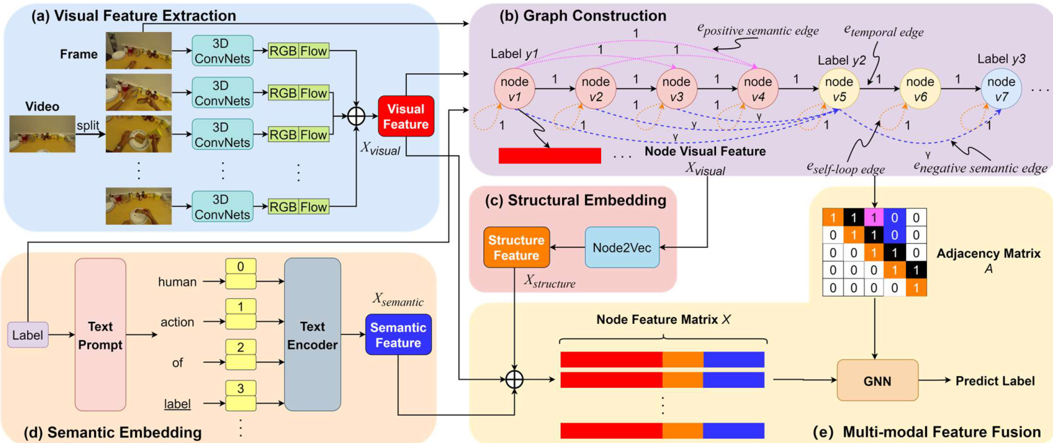
Fig. 1 Overview of the pipeline for Semantic 2 Graph. (a) Extracting visual features from video frames. (b) An instance of a videobased graph. (c) Encoding node neighborhood information as structural features. (d) Encoding the label text to obtain semantic features. (e) A GNNs is trained to fusion multi-modal features to predict node labels.

图 1: Semantic 2 Graph流程概览。(a) 从视频帧中提取视觉特征。(b) 基于视频的图结构实例。(c) 将节点邻域信息编码为结构特征。(d) 对标签文本进行编码以获取语义特征。(e) 训练GNNs (Graph Neural Networks)融合多模态特征以预测节点标签。

Step (e) is multi-modal feature fusion, as shown in Fig. 1(e). Its inputs include visual features from step (a), structural features from step (c), semantic features from step (d), and a directed graph from step (b). A weighted adjacency matrix is generated from the directed graph. The multi-modal feature matrix is obtained by concatenating visual features, structural features, and semantic features. A GNNs is selected as the backbone model to learn multi-modal feature fusion. The output is the node's predicted action label.

步骤 (e) 是多模态特征融合，如图 1(e) 所示。其输入包括来自步骤 (a) 的视觉特征、来自步骤 (c) 的结构特征、来自步骤 (d) 的语义特征以及来自步骤 (b) 的有向图。根据有向图生成加权邻接矩阵。通过拼接视觉特征、结构特征和语义特征获得多模态特征矩阵。选择 GNNs 作为主干模型来学习多模态特征融合。输出为节点的预测动作标签。

2.3 Graph construction of video

2.3 视频的图结构构建

This section is to describe how a video is transformed into our defined graph. The defined graph is a directed graph $\mathcal{D}i\mathcal{G}(\mathcal{V},\mathcal{E})$ composed of a set of nodes $\mathcal{V}$ and a set of edges $\mathcal{E}$ . Compared with undirected graph, directed graph are more conducive to modeling temporal or order relations [18].

本节将描述如何将视频转化为我们定义的图结构。该图是一个有向图 $\mathcal{D}i\mathcal{G}(\mathcal{V},\mathcal{E})$，由节点集 $\mathcal{V}$ 和边集 $\mathcal{E}$ 组成。与无向图相比，有向图更有利于建模时序或顺序关系 [18]。

2.3.1 Node

2.3.1 节点 (Node)

The input is a set of untrimmed videos. A frame $f_{t}$ is the frame at time slot $t$ in the video. Video $\nu$ is a set of $f_{t}$ , where the set contains $T$ frames. As shown in Fig. 1 (b) that video $\nu$ is represented by a directed graph $\mathcal{D}i\boldsymbol{\mathcal{G}}(\boldsymbol{\mathcal{V}},\boldsymbol{\mathcal{E}})$ . A frame f in a video is represented by a node $\mathbfcal{\Delta}\mathbfcal{\Psi}$ in the directed graph. In other words, a directed graph with $T$ nodes represents a video with $T$ frames. Directed graphs can explicitly model temporal relations in videos, and can also model action-order relations. Especially irreversible action pairs, such as door opening-closing, egg breaking-stirring.

输入是一组未经修剪的视频。帧 $f_{t}$ 是视频中时间槽 $t$ 的帧。视频 $\nu$ 是一组 $f_{t}$，其中集合包含 $T$ 帧。如图1(b)所示，视频 $\nu$ 由有向图 $\mathcal{D}i\boldsymbol{\mathcal{G}}(\boldsymbol{\mathcal{V}},\boldsymbol{\mathcal{E}})$ 表示。视频中的帧f由有向图中的节点 $\mathbfcal{\Delta}\mathbfcal{\Psi}$ 表示。换句话说，具有 $T$ 个节点的有向图表示具有 $T$ 帧的视频。有向图可以显式建模视频中的时间关系，也可以建模动作顺序关系，尤其是不可逆的动作对，例如开门-关门、打蛋-搅拌。

For each node, there is a label $y$ converted from the label of the represented frame. Without loss of generality, we assume that the video has pre-obtained frame-level action annotations by some methods, such as frame-based methods [2, 6, 14], segment-based methods, or proposal-based methods [1, 3, 8, 19]. In addition, each node has three attributes that are multimodal features extracted from frames. The details of extracting frame features are subsequently specified in Section 2.4.

对于每个节点，都有一个从所代表帧的标签转换而来的标签 $y$。不失一般性，我们假设视频已通过某些方法（例如基于帧的方法 [2, 6, 14]、基于片段的方法或基于提案的方法 [1, 3, 8, 19]）预先获取了帧级动作标注。此外，每个节点具有三个属性，这些属性是从帧中提取的多模态特征。提取帧特征的细节将在第2.4节中具体说明。

2.3.2 Edge

Videos contain not only rich sequential dependencies between frames, but also potential semantic relations, such as captions, context, action interactions, object categories, and more. These dependencies are crucial for a comprehensive understanding of video [19].

视频不仅包含帧间丰富的时序依赖关系，还蕴含潜在的语义关联，如字幕、上下文、动作交互、物体类别等。这些依赖关系对于全面理解视频内容至关重要 [19]。

To enhance the graph representation learning of videos, there are two types of edges in the directed graph, temporal edges, and semantic edges, as shown in Fig. 1 (b). In addition, to enhance the complexity of a graph and preserve the features of the node itself, another type of edge self-loop is added to the directed graph [19]. Each edge has a weight value determined by the type of edge.

为增强视频的图表示学习能力，有向图中包含两种边类型：时序边和语义边，如图1(b)所示。此外，为提升图的复杂度并保留节点自身特征，有向图中还添加了另一种自循环边类型[19]。每条边的权重值由其边类型决定。

Temporal edge. It is the baseline edge of the directed graph to represent the sequential order of frames. Intuitively, it reflects the temporal adjacency relation between two neighbor nodes [1, 6, 19, 20]. In general, the weight of the temporal edge is set to 1. The temporal edge is formulated as

时序边。它是用于表示帧序列顺序的有向图基线边，直观地反映了相邻节点间的时间邻接关系 [1, 6, 19, 20]。通常时序边的权重设为1，其数学表达式为

$$
\begin{array}{l}{{e_{t e m p o r a l}=(\boldsymbol{\nu}{t},\boldsymbol{\nu}{t+1}),~t\in[1,{T}-1]}}\ {{\boldsymbol{w}_{t e m p o r a l}=1}}\end{array}
$$

Semantic edge. It is to model the potential semantic relations of videos [1]. Semantic edges are categorized into two types, namely, positive semantic edge and negative semantic edge. Positive semantic edge is to group nodes with identical labels while negative semantic edge is to distinguish nodes with different labels. A simple rule to construct semantic edges is to add either positive or negative edges between any two nodes based on their labels. However, the size of edges is $0(\mathcal{V}^{2})$ resulting in the consumption of memory space and computing time. We here propose a semantic edge construction method to optimize the directed graph with minimum edges and sufficient semantic relations of video.

语义边缘。它用于建模视频的潜在语义关系[1]。语义边缘分为两种类型，即正语义边缘和负语义边缘。正语义边缘是将具有相同标签的节点分组，而负语义边缘是区分具有不同标签的节点。构建语义边缘的一个简单规则是根据节点的标签在任意两个节点之间添加正边缘或负边缘。然而，边缘的大小为$0(\mathcal{V}^{2})$，会导致内存空间和计算时间的消耗。我们在此提出一种语义边缘构建方法，以优化具有最少边缘和充分视频语义关系的有向图。

Each node has a sequence identifier which is the same as the ID of the representative frame. The smaller the ID number, the earlier the frame in a video. For each node, $\mathbf{\nabla}\cdot\boldsymbol{\psi}{i}$ adds a positive edge to the following nodes $\boldsymbol{\mathbf{\mathit{\sigma}}}^{\mathcal{\leftrightarrow}{j}}$ whose $j>i$ until the label of $\boldsymbol{\mathbf{\mathit{\sigma}}}^{\mathcal{\leftrightarrow}}$ is different from the label of $\mathbf{\nabla}\cdot\boldsymbol{\nu}{i}$ and add a negative edge to $\boldsymbol{\cdot}\boldsymbol{\cdot}_{j}$ Positive semantic edge and negative semantic edge are defined as

每个节点都有一个序列标识符，该标识符与代表帧的ID相同。ID号越小，表示该帧在视频中出现的时间越早。对于每个节点，$\mathbf{\nabla}\cdot\boldsymbol{\psi}{i}$ 会向后续节点 $\boldsymbol{\mathbf{\mathit{\sigma}}}^{\mathcal{\leftrightarrow}{j}}$（其中 $j>i$）添加正向边，直到 $\boldsymbol{\mathbf{\mathit{\sigma}}}^{\mathcal{\leftrightarrow}}$ 的标签与 $\mathbf{\nabla}\cdot\boldsymbol{\nu}{i}$ 的标签不同为止，并向 $\boldsymbol{\cdot}\boldsymbol{\cdot}_{j}$ 添加负向边。
Self-loop edge. It is referring to the settings of the MIGCN model that each node adds a self-loop edge with a weight of 1. During message aggregation, the self-loop edge maintains the node's information [19]. The self-loop edge is formulated as

自循环边 (self-loop edge)。这指的是 MIGCN 模型中每个节点添加一条权重为 1 的自循环边的设置。在信息聚合过程中，自循环边用于保持节点的原始信息 [19]。其数学表达式为

$$
\begin{array}{r l}&{{{e_{s e l f-l o o p}}}=(\psi_{t},{{\nu_{t}}}),t\in[1,T]}\ &{{{w_{s e l f-l o o p}}}=1}\end{array}
$$

2.4 多模态特征

Video contents are extracted as features and added to nodes in the graph. They are visual, structure, and semantic features, belonging to low-level, middle-level, and high-level features [14], respectively, as shown in Fig. 1.

视频内容被提取为特征并添加到图中的节点。这些特征包括视觉、结构和语义特征，分别属于低层、中层和高层特征 [14]，如图 1 所示。

Visual feature. Visual features are the most fundamental and important features. It captures the appearance information, such as color, texture, and motion, which are essential for understanding actions in videos. In our method, it is an image embedding containing RGB and optical-flow information of each frame in a video, as shown in Fig. 1 (a). Optical flow estimation techniques to extract motion features aim at capturing temporal dynamics. Many visual feature extractors have been developed, such as I3D, C3D, ViT, etc. [1, 20]. In this study, we use I3D to extract visual features. The I3D feature extractor takes a video $\nu_{i}$ input and outputs two tensors with 1024-dimensional features: for RGB and optical-flow streams. Visual features concatenate RGB and optical-flow feature tensors. Visual feature is represented by $\mathbf{X}{v i s u a l}\in\mathbb{R}^{\mathbf{T}\times\mathbf{D}{v i s u a l}}$ , $\mathrm{D}_{v i s u a l}=2048$ .

视觉特征。视觉特征是最基础且重要的特征，它捕捉了颜色、纹理和运动等外观信息，这些对于理解视频中的动作至关重要。在我们的方法中，它是一个包含视频每帧RGB和光流信息的图像嵌入，如图1(a)所示。用于提取运动特征的光流估计技术旨在捕捉时间动态。目前已开发出许多视觉特征提取器，如I3D、C3D、ViT等[1,20]。本研究采用I3D提取视觉特征。I3D特征提取器以视频$\nu_{i}$为输入，输出两个1024维特征张量：分别对应RGB流和光流。视觉特征由RGB与光流特征张量拼接而成，表示为$\mathbf{X}{v i s u a l}\in\mathbb{R}^{\mathbf{T}\times\mathbf{D}{v i s u a l}}$，其中$\mathrm{D}_{v i s u a l}=2048$。

$$
\mathrm{X}{v i s u a l,i}=\mathrm{I}3\mathrm{D}(v_{i})
$$

Structure Feature. It is the node embedding transferring features into a low-dimensional space with minimum loss of information of the neighborhood nodes. General structure features are the structure of a graph. In this paper, structure features reflect the structural properties of a graph.

结构特征。它是将节点嵌入到低维空间中，同时最小化邻域节点信息损失的特征。通用结构特征指的是图的结构。本文中，结构特征反映图的结构属性。

The graph-structured representation of video provides valuable information about the temporal relation between different frames or video segments. The graph structure can capture both temporal coherence and action order, which allows us to model the sequential nature of actions in videos. The structural properties are relational properties of a video, including intrinsic sequence-structure properties and semantic properties. They are preserved by our designed temporal edge and semantic edge. See Section 2.3.2 for details. Structural features provide important action order information. The combination of structural features enables our method to model the dynamic evolution of actions over time and helps to accurately segment actions and recognize boundaries.

视频的图结构表示提供了关于不同帧或视频片段间时序关系的宝贵信息。图结构能同时捕捉时序连贯性和动作顺序，使我们能够对视频中动作的序列特性进行建模。结构属性是视频的关系属性，包括内在序列结构属性和语义属性。这些属性通过我们设计的时间边 (temporal edge) 和语义边 (semantic edge) 得以保留，详见第2.3.2节。结构特征提供了重要的动作顺序信息，其组合使我们的方法能够建模动作随时间的动态演化，并有助于准确分割动作和识别边界。

In computer vision, most of the existing methods [15, 19, 21] use Recurrent Neural Networks (RNN) sequence models such as GRU, BiGRU [19], LSTM or Transformer [15, 21] to capture the intrinsic sequence-structure properties of videos, and then to reason the mapping relation between frame and action. However, the methods mentioned above are not suitable for graphs. The reason is that they are not good at dealing with nonEuclidean forms of graphs.

在计算机视觉领域，现有大多数方法[15,19,21]采用GRU、BiGRU[19]、LSTM或Transformer[15,21]等循环神经网络(RNN)序列模型来捕捉视频固有的序列结构特性，进而推理帧与动作间的映射关系。然而上述方法并不适用于图结构数据，因其难以有效处理图的非欧几里得形式。

For a graph, the structure features are obtained by using a node embedding algorithm. There are many node embedding algorithms, such as DeepWalk for learning the similarity of neighbors, LINE for learning the similarity of first-order and second-order neighbors, and node2vec [22] for learning the similarity of neighbors and structural similarity.

对于一张图，其结构特征通过节点嵌入 (node embedding) 算法获取。现有多种节点嵌入算法，例如 DeepWalk 用于学习邻居相似性，LINE 用于学习一阶和二阶邻居相似性，以及 node2vec [22] 用于学习邻居相似性和结构相似性。

In this paper, node2vec is used to get the structural features, as shown in Fig. 1 (c). The structure feature is represented by $\mathbf{\calX}{s t r u c t u r e}\in\mathbb{R}^{\mathbf{T}\times\mathbf{D}{s}}$ ೞ೟ೝೠ೎೟ೠೝ೐, where dimension $\mathrm{D}_{s t r u c t u r e}=128$ .

本文使用node2vec获取结构特征，如图1 (c) 所示。结构特征表示为 $\mathbf{\calX}{s t r u c t u r e}\in\mathbb{R}^{\mathbf{T}\times\mathbf{D}{s}}$ ೞ೟ೝೠ೎೟ೠೝ೐，其中维度 $\mathrm{D}_{s t r u c t u r e}=128$。

where the node attributes of the graph $\mathcal{D}i\mathcal{G}(\mathcal{V},\mathcal{E})$ are only visual features.

其中图 $\mathcal{D}i\mathcal{G}(\mathcal{V},\mathcal{E})$ 的节点属性仅为视觉特征。

Semantic feature. It is the language embedding of each frame of a video, such as textual prompt [16] or the semantic information of label-text [4], as shown in Fig. 1 (d). Semantic features provide a higher-level understanding of actions occurring in videos. Furthermore, semantic features can assist in handling challenging scenarios, such as ambiguous or rare actions, by providing additional cues for disambiguation. CLIP [15] and ActionCLIP [4] are common approaches to getting semantic features. In this study, we use ActionCLIP.

语义特征。它是视频每一帧的语言嵌入，例如文本提示 [16] 或标签文本的语义信息 [4]，如图 1 (d) 所示。语义特征提供了对视频中发生动作的更高级理解。此外，语义特征可以通过提供额外的消歧线索，帮助处理具有挑战性的场景，例如模糊或罕见的动作。CLIP [15] 和 ActionCLIP [4] 是获取语义特征的常见方法。在本研究中，我们使用 ActionCLIP。

Following the ActionCLIP model proposed by Wang et al. [4], based on the filling locations, the filling function $\mathcal{T}$ has the following three varieties:

遵循Wang等人[4]提出的ActionCLIP模型，根据填充位置的不同，填充函数$\mathcal{T}$可分为以下三种变体：

Prefix prompt [4]: label, a video of action; ● Cloze prompt [4]: this is label, a video of action; ● Suffix prompt [4]: human action of label.

前缀提示 [4]: label, 一段动作视频;
● 填空提示 [4]: 这是 label, 一段动作视频;
● 后缀提示 [4]: label 的人类动作。

ActionCLIP uses the label-text to fill the sentence template ${ Z} = {z{I}, ...,~z_{k}}$ with the filling function $\mathcal{T}$ to obtain the prompted textual [4].

ActionCLIP 使用标签文本通过填充函数 $\mathcal{T}$ 填充句子模板 ${ Z} = {z{I}, ...,~z_{k}}$ 以获取提示性文本 [4]。

$$
\mathcal{Y}^{\prime}=\mathcal{T}(\mathcal{Y},\mathrm{Z})
$$

Compared with only label words, the prompt-based method expands the label-text, which enhances the semantic features. A text encoder encodes is to obtain semantic features, which are used as language supervision information to improve the performance of vision tasks. The semantic feature is represented by $\mathrm{X}{s e m a n t i c}\in\mathbb{R}^{\mathrm{T}\times\mathrm{D}{s e m a n t i c}}$ , where dimension $\mathrm{D}_{s e m a n t i c}=512$ .

相比仅使用标签词，基于提示词 (prompt) 的方法扩展了标签文本，从而增强了语义特征。文本编码器通过编码获得语义特征，这些特征作为语言监督信息用于提升视觉任务的性能。语义特征表示为 $\mathrm{X}{s e m a n t i c}\in\mathbb{R}^{\mathrm{T}\times\mathrm{D}{s e m a n t i c}}$ ，其中维度 $\mathrm{D}_{s e m a n t i c}=512$ 。

$$
\mathrm{X}_{s e m a n t i c}=\mathrm{Text_Encoder}(\mathcal{Y}^{\prime})
$$

As shown in Fig. 1 (e) that the multi-modal feature of the node is

如图1(e)所示，节点的多模态特征

$$
\begin{array}{r}{\mathbf{X}=\mathbf{X}{\mathit{v i s u a l}}\left|\mathbf{X}{\mathit{s t r u c t u r e}}\right|\mathbf{X}_{\mathit{s e m a n t i c}}}\end{array}
$$

where $\parallel$ represents a concatenation operation.

其中 $\parallel$ 表示连接操作。

2.5 Graph construction algorithms

2.5 图构建算法

Here is the algorithm pseudo code to describe how to create a directed graph from a video. In Algorithm 1, the input is a video $\nu$ and its set of action labels $\mathcal{Y}$ , and the output is a directed graph. It is divided into 7 steps as follows:

以下是描述如何从视频创建有向图的算法伪代码。在算法1中，输入为视频$\nu$及其动作标签集合$\mathcal{Y}$，输出为有向图。该算法分为以下7个步骤：

Step 1. Initialization (see lines 1-2). Create an empty directed graph $\mathcal{D}i\mathcal{G}(\mathcal{V},\mathcal{E})$ consisting of node set $\mathcal{V}$ and edge set ℰ. Split the video $\nu$ into a set of frames ${f_{1},...,f_{\mathrm{T}}}$ .

步骤 1. 初始化 (见第 1-2 行)。创建一个由节点集 $\mathcal{V}$ 和边集 ℰ 组成的空有向图 $\mathcal{D}i\mathcal{G}(\mathcal{V},\mathcal{E})$。将视频 $\nu$ 分割为帧集合 ${f_{1},...,f_{\mathrm{T}}}$。

Step 2. Create nodes (see lines 3-5). Creates a node ${\mathbf{}}{\mathbf{}}{\mathbf{}}{\mathbf{}}^{}{\mathbf{\Xi}}{\mathbf{\Xi}}^{\prime}{\mathbf{{i}}}$ based on frame-level. Node $\upsilon_{\mathrm{i}}$ represents video frame $f_{\mathrm{i}}$ , so the label of node $\upsilon_{\mathrm{i}}$ is the label $y_{\mathrm{i}}$ of video frame $f_{\mathrm{i}}$ . Then add node $\upsilon_{\mathrm{i}}$ to a node-set $\mathcal{V}$ .

步骤2. 创建节点（见第3-5行）。基于帧级别创建节点 ${\mathbf{}}{\mathbf{}}{\mathbf{}}{\mathbf{}}^{}{\mathbf{\Xi}}{\mathbf{\Xi}}^{\prime}{\mathbf{{i}}}$ 。节点 $\upsilon_{\mathrm{i}}$ 代表视频帧 $f_{\mathrm{i}}$ ，因此节点 $\upsilon_{\mathrm{i}}$ 的标签即为视频帧 $f_{\mathrm{i}}$ 的标签 $y_{\mathrm{i}}$ 。随后将节点 $\upsilon_{\mathrm{i}}$ 添加至节点集 $\mathcal{V}$ 。

Step 3. Create temporal edges (see lines 6-9). Traverse the node set ${\nu_{2},...,\nu_{\mathrm{{T}}}}$ . Then a temporal edge $(\pmb{\nu}{\mathrm{{i}-1}},\pmb{\nu}{\mathrm{{i}}})$ with weight 1 from node $\scriptstyle v_{\mathrm{i-1}}$ to node ${\mathbf{\nabla}}{\cdot}v_{\mathrm{i}}$ is added to the edge set $\mathcal{E}$ .

第3步：创建时序边（见第6-9行）。遍历节点集 ${\nu_{2},...,\nu_{\mathrm{{T}}}}$，随后向边集 $\mathcal{E}$ 添加一条从节点 $\scriptstyle v_{\mathrm{i-1}}$ 到节点 ${\mathbf{\nabla}}{\cdot}v_{\mathrm{i}}$、权重为1的时序边 $(\pmb{\nu}{\mathrm{{i}-1}},\pmb{\nu}_{\mathrm{{i}}})$。

Algorithm 1 Video to a Directed Graph

算法 1：视频转有向图

| 输入：加载视频 v ∈ V 和真实标签 Y = {y1, ..., yT} |
| 输出：有向图 DiG(V, ε) |

| // 步骤 1：初始化 |
| 1: | 创建空有向图 DiG(V, ε) |
| 2: | 将视频分割为帧集合 {f1, ..., fT} |

| // 步骤 2：创建节点 |
| 3: | for i ∈ [1, T] do |
| 4: | 创建节点 vi 并将 V ← 添加节点 vi |
| 5: | end for |

| // 步骤 3：创建时序边 |
| 6: | for i ∈ [2, T] do |
| 7: | ε ← 添加时序边 etemporal = (vi-1, vi) 且 wtemporal = 1 |
| 8: | end if |
| 9: | end for |

| // 步骤 4：创建正向语义边 |
| 10: | node_group = {v1} |
| 11: | for i ∈ [2, T] do |
| 12: | if yi == yi-1 then |
| 13: | for vj in node_group do |
| 14: | if j < i-1 then |
| 15: | ε ← 添加正向语义边 epositive_semantic = (vj, vi) 且 wpositive_semantic = 1 |
| 16: | end if |
| 17: | end for |
| 18: | else node_group = {} |
| 19: | end if |
| 20: | node_group ← 添加 vi |
| 21: | end for |

| // 步骤 5：创建负向语义边 |
| 22: | node_group = {v1} |
| 23: | for i ∈ [2, T] do |
| 24: | if yi ≠ yi-1 then |
| 25: | for vj in node_group do |
| 26: | if i-j ≠ 1 then |
| 27: | ε ← 添加负向语义边 enegative_semantic = (vj, vi) 且 wnegative_semantic = 1 |
| 28: | end if |

Step 4. Create positive semantic edges (see lines 10-21). First, create a node group node_group whose initial value is node $\upsilon_{1}$ . Then, traverse the node set ${\boldsymbol{v}{2},...,\boldsymbol{v}{\mathrm{T}}}$ . If the label $y_{\mathrm{i}}$ of the current node ${\mathbf{}}\cdot{\mathbf{}}{i}$ is the same as the label $y_{\mathrm{i-l}}$ of the previous node $\scriptstyle{\upsilon_{\mathrm{i-1}}}$ , then further traverse the node group. If node $\boldsymbol{\cdot}\boldsymbol{\cdot}$ in node_group is not a neighbor of node ${\mathbfit{\Delta}}{\cdot\mathbfit{\partial}}{\boldsymbol{\psi}}{\mathrm{{i}}}$ (that is, $j\neq i{-}I$ ), then edge set $\mathcal{E}$ is added with a positive semantic edge $(\upsilon_{\mathrm{j}},\upsilon_{\mathrm{i}})$ with weight 1 from node $\boldsymbol{\cdot}\boldsymbol{\cdot}$ to node ${\mathbf{}}{\mathbf{}}{\mathbf{}}{\mathbf{}}^{}{\mathbf{\Xi}}{\mathbf{\Xi}}^{\prime}{\mathbf{{i}}}$ . Otherwise, node_group is emptied. Finally, node $\upsilon_{\mathrm{i}}$ is added to node_group.

步骤4. 创建正向语义边（见代码10-21行）。首先创建初始值为节点$\upsilon_{1}$的节点组node_group，随后遍历节点集${\boldsymbol{v}{2},...,\boldsymbol{v}{\mathrm{T}}}$。若当前节点${\mathbf{}}\cdot{\mathbf{}}{i}$的标签$y_{\mathrm{i}}$与前一个节点$\scriptstyle{\upsilon_{\mathrm{i-1}}}$的标签$y_{\mathrm{i-l}}$相同，则进一步遍历该节点组。若node_group中的节点$\boldsymbol{\cdot}\boldsymbol{\cdot}$不是节点${\mathbfit{\Delta}}{\cdot\mathbfit{\partial}}{\boldsymbol{\psi}}{\mathrm{{i}}}$的邻居（即$j\neq i{-}I$），则向边集$\mathcal{E}$添加一条从节点$\boldsymbol{\cdot}\boldsymbol{\cdot}$到节点${\mathbf{}}{\mathbf{}}{\mathbf{}}{\mathbf{}}^{}{\mathbf{\Xi}}{\mathbf{\Xi}}^{\prime}{\mathbf{{i}}}$、权重为1的正向语义边$(\upsilon_{\mathrm{j}},\upsilon_{\mathrm{i}})$。否则清空node_group。最后将节点$\upsilon_{\mathrm{i}}$加入node_group。

Step 5. Create negative semantic edges (see lines 21-33). Negative semantic edges and positive semantic edges have similar execution procedures. The difference is as follows: In line 26, only when the label $y_{\mathrm{i}}$ of the current node ${\mathbf{}}{\mathbf{}}{\mathbf{}}{\mathbf{}}^{}{\mathbf{\Xi}}{\mathbf{\Xi}}^{\prime}{\mathbf{{i}}}$ is different from the label yi-1 of the previous node $\scriptstyle v_{\mathrm{i-1}}$ , the node group is further traversed. Except adjacent nodes, all nodes in node_group construct a negative semantic edge with node ${\mathbf{}}{\mathbf{\mathcal{O}}{\mathrm{i}}}$ respectively. See line 28, edge set $\mathcal{E}$ is added with a negative semantic edge $(\upsilon_{\mathrm{j}},\upsilon_{\mathrm{i}})$ with weight $\upgamma$ from node $\boldsymbol{\cdot}\boldsymbol{\cdot}$ to node ${\mathbf{}}\cdot{\mathbf{}}{v_{\mathrm{i}}}$ . Then node_group is emptied.

步骤5. 创建负语义边（见21-33行）。负语义边与正语义边的执行流程相似，区别在于：第26行中，只有当当前节点 ${\mathbf{}}{\mathbf{}}{\mathbf{}}{\mathbf{}}^{}{\mathbf{\Xi}}{\mathbf{\Xi}}^{\prime}{\mathbf{{i}}}$ 的标签 $y_{\mathrm{i}}$ 与前一个节点 $\scriptstyle v_{\mathrm{i-1}}$ 的标签 yi-1 不同时，才会继续遍历节点组。除相邻节点外，节点组中所有节点分别与节点 ${\mathbf{}}{\mathbf{\mathcal{O}}{\mathrm{i}}}$ 构建负语义边。如第28行所示，边集 $\mathcal{E}$ 会添加一条从节点 $\boldsymbol{\cdot}\boldsymbol{\cdot}$ 到节点 ${\mathbf{}}\cdot{\mathbf{}}{v_{\mathrm{i}}}$ 、权重为 $\upgamma$ 的负语义边 $(\upsilon_{\mathrm{j}},\upsilon_{\mathrm{i}})$ ，随后清空节点组。

Step 6. Create self-loop edges (see lines 34-36). Traverse the node set ${\boldsymbol{v}{1},...,\boldsymbol{v}{\mathrm{T}}}$ , and add a self-loop edge $(\upsilon_{\mathrm{{i}}},\upsilon_{\mathrm{{i}}})$ with weight 1 to the node set $\mathcal{E}$ for each node ${\mathbf{}}{\mathbf{}}{\mathbf{}}{\mathbf{}}^{}{\mathbf{\Xi}}{\mathbf{\Xi}}^{\prime}{\mathbf{{i}}}$ .

步骤 6. 创建自循环边 (见代码行 34-36)。遍历节点集 ${\boldsymbol{v}{1},...,\boldsymbol{v}{\mathrm{T}}}$，为每个节点 ${\mathbf{}}{\mathbf{}}{\mathbf{}}{\mathbf{}}^{}{\mathbf{\Xi}}{\mathbf{\Xi}}^{\prime}{\mathbf{{i}}}$ 添加一条权重为 1 的自循环边 $(\upsilon_{\mathrm{{i}}},\upsilon_{\mathrm{{i}}})$ 到边集 $\mathcal{E}$。

Step 7. Get node attributes (see lines 37-41). First, extract visual features $\mathrm{X}{\nu i s u a l}$ (RGB and optical flow) from a set of frames ${f_{1},...,f_{\mathrm{T}}}$ using a visual feature extractor. Then, the visual features $\mathrm{X}{\nu i s u a l}$ are used as node attributes of the directed graph $\mathcal{D}i\mathcal{G}(\mathcal{V},\mathcal{E})$ . On $\mathcal{D}i\mathcal{G}(\mathcal{V},\mathcal{E})$ , a node embedding model is used to encode the structural features Xstructure of node neighborhoods. Semantic features $\mathrm{X}{s e m a n t i c}$ are obtained by using a textual prompt model to encode the label text $\mathcal{Y}$ of nodes. Concatenating $\mathrm{X}_{\nu i s u a l},$ Xstructure and Xsemantic compositional multi-modal features $\mathrm{X}$ as new attributes of nodes.

步骤7. 获取节点属性（见第37-41行）。首先，使用视觉特征提取器从帧序列${f_{1},...,f_{\mathrm{T}}}$中提取视觉特征$\mathrm{X}{\nu i s u a l}$（RGB和光流）。随后，将视觉特征$\mathrm{X}{\nu i s u a l}$作为有向图$\mathcal{D}i\mathcal{G}(\mathcal{V},\mathcal{E})$的节点属性。在$\mathcal{D}i\mathcal{G}(\mathcal{V},\mathcal{E})$上，采用节点嵌入模型对节点邻域的结构特征Xstructure进行编码。语义特征$\mathrm{X}{s e m a n t i c}$通过文本提示模型编码节点标签文本$\mathcal{Y}$获得。最终将$\mathrm{X}_{\nu i s u a l}$、Xstructure和Xsemantic拼接为组合多模态特征$\mathrm{X}$，作为节点的新属性。

Finally, save the directed graph $\mathcal{D}i\mathcal{G}(\mathcal{V},\mathcal{E})$ with nodes, node attributes, node labels, edges, and edge weights transferred from video $\nu$

最后，保存从视频 $\nu$ 转移而来的节点、节点属性、节点标签、边和边权重构成的有向图 $\mathcal{D}i\mathcal{G}(\mathcal{V},\mathcal{E})$。

An instance of the design of edges according to Algorithm 1 as illustrated in Fig. 2. It is worth noting that for adjacent nodes, according to the definitions of temporal and semantic edges in Section 2.3. A temporal edge and a positive semantic edge or a negative semantic edge should be added between them. But in

根据算法1设计的边实例如图2所示。值得注意的是，对于相邻节点，根据第2.3节中时间和语义边的定义，应在它们之间添加一条时间边和一条正语义边或负语义边。但在

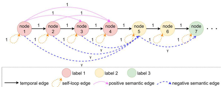
Fig. 2 An instance of an edge in a directed graph. The color of the node represents different labels. Positive semantic edges (pink dashed lines) and negative semantic edges (blue dashed lines) are examples of semantic edges. The edge's value indicates its weight.

图 2: 有向图中一条边的示例。节点颜色代表不同标签。粉色虚线表示正向语义边 (positive semantic edges) ，蓝色虚线表示负向语义边 (negative semantic edges) 。边的数值代表其权重。

Algorithm 1 (see lines 6 and 7), only the temporal edges that are used to save the time series information of the video are added. See line 14, the purpose of setting the condition $j<i-1$ is to avoid adding positive semantic edges $(\pmb{\upsilon}{i-1},\pmb{\upsilon}{i})$ . See line 26, the purpose of setting the condition $i{-}j\neq1$ is to avoid adding negative semantic edges $(\pmb{\upsilon}{i-1},\pmb{\upsilon}_{i})$ . As shown in Fig. 2, nodes 1 and 2, nodes 2 and 3, nodes 3 and 4, nodes 4 and 5, and nodes 5 and 6 have only temporal edges.

算法 1 (见第 6 和 7 行), 仅添加用于保存视频时间序列信息的时间边。见第 14 行, 设置条件 $j<i-1$ 的目的是避免添加正向语义边 $(\pmb{\upsilon}{i-1},\pmb{\upsilon}{i})$。见第 26 行, 设置条件 $i{-}j\neq1$ 的目的是避免添加负向语义边 $(\pmb{\upsilon}{i-1},\pmb{\upsilon}_{i})$。如图 2 所示, 节点 1 和 2、节点 2 和 3、节点 3 和 4、节点 4 和 5 以及节点 5 和 6 之间仅有时间边。

For non-adjacent nodes, a positive semantic edge and a negative semantic edge should be added between them. But in Algorithm 1 (see lines 12 to 19), only non-adjacent nodes with the same label are added positive semantic edges. See lines 23 to 27, only non-adjacent nodes with the different label are added negative semantic edges. As shown in Fig. 2, nodes 1 and 3, nodes 1 and 4 and nodes 2 and 4 is positive semantic edges. While nodes 1 and 5, nodes 2 and 5, nodes 3 and 5 and nodes 5 and 7 is negative semantic edges.

对于非相邻节点，应在它们之间添加一条正语义边和一条负语义边。但在算法1中（见第12至19行），仅对具有相同标签的非相邻节点添加了正语义边。见第23至27行，仅对具有不同标签的非相邻节点添加了负语义边。如图2所示，节点1和3、节点1和4以及节点2和4之间存在正语义边，而节点1和5、节点2和5、节点3和5以及节点5和7之间存在负语义边。

For human-annotated videos, two consecutive frames may have different labels despite their similar visual features. To enhance the boundaries of semantic labels in the graph, the weight of positive semantic edges is set to 1 and the weight of negative semantic edges is set to $\upgamma$ . In Fig. 2, positive semantic edges enhance the semantic relation that node 4 belongs to the same label as nodes 1, 2, and 3. Negative semantic edges enhance the semantic relation between node 5 and nodes 1, 2, and 3 belonging to different labels. In summary, semantic edges also help in label class prediction for two adjacent nodes whose true labels are not identical.

对于人工标注的视频，连续两帧可能视觉特征相似但标签不同。为增强图中语义标签的边界，正语义边的权重设为1，负语义边的权重设为$\upgamma$。在图2中，正语义边强化了节点4与节点1、2、3属于同一标签的语义关系，负语义边则强化了节点5与节点1、2、3属于不同标签的语义关系。综上所述，语义边也有助于预测两个真实标签不同但相邻节点的标签类别。

In a graph with only temporal edges, a node has only two neighbors, so the message aggregation within 1 hop is limited. Moreover, if the nodes want to aggregate messages from more nodes or more distant nodes, the model needs to go through multi-hop and expensive computation. Conversely, semantic edges allow the model to be implemented within 1 hop. Hence, semantic edges significantly reduce the computational cost of message aggregation in GNNs [1].

在仅含时序边的图中，节点仅有两个邻居，因此单跳内的消息聚合受限。此外，若节点需聚合更多或更远节点的信息，模型需进行多跳且昂贵的计算。反之，语义边可使模型在单跳内实现聚合。因此，语义边能显著降低图神经网络 (GNN) 中消息聚合的计算成本 [1]。

2.6 Graph-based fusion model

2.6 基于图(Graph)的融合模型

In this paper, we treat video action segmentation and recognition as a node classification problem on graphs. We need to define a weighted adjacency matrix𝒜 with weight that relies on the three types of edges and their weights proposed in

在本论文中，我们将视频动作分割与识别视为图结构上的节点分类问题。需要定义一个加权邻接矩阵𝒜，其权重取决于文献[20]提出的三类边及其权重。

To this end, we use a Graph Neural Network (GNN) model $\mathcal{F}=f(\mathrm{X},\mathcal{A})$ as the backbone model to fuse the multi-modal features of nodes. Specifically, it is a two-layer graph convolutional neural network (GCN), which is a spatial-based model suitable for processing directed graphs [17, 18].

为此，我们采用图神经网络 (Graph Neural Network, GNN) 模型 $\mathcal{F}=f(\mathrm{X},\mathcal{A})$ 作为骨干网络来融合节点的多模态特征。具体而言，该模型是一个基于空间域的双层图卷积神经网络 (GCN) ，适用于处理有向图 [17, 18]。

Since undirected graphs are a special case of directed graphs, the undirected graph convolution operator does not work with directed graphs. In a directed graph, the degree of a node is divided into out-degree and in-degree. Directed graphs need to perform convolution operations on them separately. Chung [24] gives the definition of Laplacian for a directed graph as follows

由于无向图是有向图的一种特殊情况，无向图卷积算子不适用于有向图。在有向图中，节点的度分为出度和入度。有向图需要分别对它们进行卷积运算。Chung [24] 给出了有向图的拉普拉斯算子定义如下

$$
{\cal L}=I_{T}-\frac{\phi^{\frac{1}{2}}\mathcal{P}\phi^{\frac{-1}{2}}+\phi^{\frac{-1}{2}}\mathcal{P}^{*}\phi^{\frac{1}{2}}}{2}
$$

where $I_{T}$ is the identity matrix, $\phi$ is a diagonal matrix, $\mathcal{P}$ is a transition probability matrix and $\mathcal{P}^{*}=\mathcal{P}^{T}$ is the conjugated transpose matrix [18, 24]. $\phi(\pmb{v}{\mathrm{{i}}},\pmb{v}{\mathrm{{i}}})=\phi(\pmb{v}{\mathrm{{i}}})$ and $\begin{array}{r}{\sum_{\nu_{\mathrm{i}}}\phi(\nu_{\mathrm{i}})=}\end{array}$ 1. $\begin{array}{r}{\phi=\frac{1}{N}}\end{array}$ the Perron vector of $\mathcal{P}$ [24]. $\mathcal{P}$ for a weighted directed graph is defined as [24]

其中 $I_{T}$ 是单位矩阵，$\phi$ 是对角矩阵，$\mathcal{P}$ 是转移概率矩阵，$\mathcal{P}^{*}=\mathcal{P}^{T}$ 为共轭转置矩阵 [18, 24]。$\phi(\pmb{v}{\mathrm{{i}}},\pmb{v}{\mathrm{{i}}})=\phi(\pmb{v}{\mathrm{{i}}})$ 且 $\begin{array}{r}{\sum_{\nu_{\mathrm{i}}}\phi(\nu_{\mathrm{i}})=}\end{array}$ 1。当 $\begin{array}{r}{\phi=\frac{1}{N}}\end{array}$ 时，$\phi$ 是 $\mathcal{P}$ 的 Perron 向量 [24]。加权有向图的 $\mathcal{P}$ 定义为 [24]

$$
\mathcal{P}(\nu_{\mathrm{i}},\nu_{\mathrm{j}})=\frac{\mathcal{W}{\mathrm{i,j}}}{\sum_{\mathrm{k}}w_{\mathrm{i,k}}}
$$

where $k$ is the number of neighbor nodes of ${\mathbf{}}\cdot{\mathbf{}}_{i}$ .

其中 $k$ 是 ${\mathbf{}}\cdot{\mathbf{}}_{i}$ 的相邻节点数量。

According to the Laplace formula mentioned above, Li et al. [18] described in detail the directed graph convolution operator considering the out-degree and in-degree, as follows

根据上述拉普拉斯公式，Li等人[18]详细描述了考虑出度和入度的有向图卷积算子，如下所示

$$
\mathsf{D}{\mathrm{{DG}}}(\mathcal{A})=\frac{\widetilde{\mathrm{D}}{\mathrm{{out}}}^{\frac{-1}{2}}(\tilde{\mathcal{A}}+\tilde{\mathcal{A}}^{\mathrm{T}})\widetilde{\mathrm{D}}_{\mathrm{{out}}}^{\frac{-1}{2}}}{2}
$$

where $\tilde{\mathcal{A}}=\mathcal{A}+I_{T}$ [18]. $\widetilde{D}{o u t}$ and $\widetilde{D}{i n}$ are the out-degree matrix and in-degree matrix, respectively. $\begin{array}{r}{\widetilde{D}{o u t}(i,i)=\sum_{j}\tilde{A}{i j}}\end{array}$ and $\begin{array}{r}{\widetilde{D}{i n}(j,j)=\sum_{i}\tilde{A}_{i j}}\end{array}$ .

其中 $\tilde{\mathcal{A}}=\mathcal{A}+I_{T}$ [18]。$\widetilde{D}{o u t}$ 和 $\widetilde{D}{i n}$ 分别为出度矩阵和入度矩阵。$\begin{array}{r}{\widetilde{D}{o u t}(i,i)=\sum_{j}\tilde{A}{i j}}\end{array}$ 且 $\begin{array}{r}{\widetilde{D}{i n}(j,j)=\sum_{i}\tilde{A}_{i j}}\end{array}$。

3 Experiments

3 实验

3.1 Datasets

3.1 数据集

To evaluate our method, we perform experiments on two action datasets of food preparation. Table 1 displays the basic information for the two benchmark datasets.

为了评估我们的方法，我们在两个食物准备动作数据集上进行了实验。表 1: 展示了这两个基准数据集的基本信息。

GTEA. Georgia Tech Egocentric Activity (GTEA) datasets consist of a first-person instructional video of food preparation in a kitchen environment. It has 28 videos with an average length of 1 minute and 10 seconds [15]. Each video is split into frame sets at 15 fps [15]. Each video has an average of 20 action instances, and each frame is annotated with 11 action categories (including background) [15]. Our method is evaluated using a 4-fold cross-validation average for this dataset [15].

GTEA。Georgia Tech Egocentric Activity (GTEA) 数据集包含厨房环境中食物准备的第一人称教学视频，共28段平均时长1分10秒的视频 [15]。视频以15帧/秒的速率分割为帧序列 [15]，每段视频平均包含20个动作实例，每帧标注了11个动作类别（含背景类别）[15]。本数据集采用4折交叉验证平均值进行评估 [15]。

50Salads. This dataset includes instructional videos of 25 testers preparing two mixed salads in a kitchen environment [14]. It contains 50 videos with an average length of 6 minutes and 24 seconds [14]. Each video is also split into frame sets at 15 fps. Each frame is labeled with 19 action categories (including background), and each video has 20 action instances on average [14].

50Salads。该数据集包含25名测试者在厨房环境中制作两份混合沙拉的指导视频[14]，共50段视频，平均时长6分24秒[14]。每段视频还以15帧/秒的速率分割为帧集，每帧标注了19个动作类别（含背景类别），平均每段视频包含20个动作实例[14]。

Table 1 Datasets

表 1: 数据集

数据集	视频数量	帧数 (最大)	帧数 (最小)	帧数 (平均)	动作类别数
GTEA	28	2009	634	1321	11
50Salads	50	18143	7804	12973	19

3.2 Evaluation metrics

3.2 评估指标

Following previous works [3, 15, 21, 33], we used the following metrics for evaluation: node-wise accuracy (Acc.), segmental edit score (Edit), and segmental overlap F1 score. Node-wise accuracy corresponds to the frame-wise accuracy of the video, which is the most used metric in action segmentation. Segmental edit score is used to compensate for the lack of nodewise accuracy for over-segmentation. Segmental overlap F1 score is used to evaluate the quality of the prediction, with the thresholds of 0.1, 0.25, and 0.5 $(\mathrm{F}1@10$ , F1@25, F1@50) respectively. Additionally, we also use Top-1 and Top-5 to evaluate our method for action recognition.

遵循先前的研究 [3, 15, 21, 33]，我们采用以下指标进行评估：节点准确率 (Acc.)、分段编辑分数 (Edit) 和分段重叠 F1 分数。节点准确率对应视频的帧级准确率，是动作分割中最常用的指标。分段编辑分数用于弥补节点准确率在过分割情况下的不足。分段重叠 F1 分数用于评估预测质量，阈值分别为 0.1、0.25 和 0.5 $( \mathrm{F}1@10$ , F1@25, F1@50)。此外，我们还使用 Top-1 和 Top-5 来评估方法在动作识别任务上的表现。

3.3 Implementation details

3.3 实现细节

For all datasets, each video is divided into a frameset at 15fps. We use I3D to extract RGB features and optical-flow of each frame as visual features. Due to computer resource constraints, a frame set constructs a graph every 500 frames sequentially sampled. The remaining less than 500 frames have also constructed a graph. Node2vec [22] is used in the directed graph to encode the neighborhood information of each node as structural features. For training data, we follow ActionCLIP [4] to encode the label text as semantic features. For the unlabeled test data, we first use ActionCLIP as the backbone model to predict the action classification for each frame as initial pseudolabels and corresponding prompt-based semantic features. Then, our model constructs the graph structure of the test data based on the initial pseudo-labels.

对于所有数据集，每个视频按15fps分割为帧集。我们使用I3D提取每帧的RGB特征和光流作为视觉特征。由于计算资源限制，帧集按顺序每500帧采样构建一个图结构，不足500帧的剩余帧也会单独构建一个图。在有向图中采用Node2vec [22]将各节点的邻域信息编码为结构特征。对于训练数据，我们遵循ActionCLIP [4]的方法将标签文本编码为语义特征。针对未标注的测试数据，首先以ActionCLIP为骨干模型预测每帧动作分类作为初始伪标签及基于提示词的语义特征，随后我们的模型基于初始伪标签构建测试数据的图结构。

In the training phase, a 2-layer GCN is used as the back-bone model, where the hidden layer dimension is 512 and the optimizer is Adam. The dimension of the node attribute matrix is 2816, of which the dimension of visual features, structural features, and semantic features are 2048, 128, and 512, respectively. The batch size is set to 8, which means that each batch has 8 graphs. Furthermore, the learning rate is 0.004, the weight delay is 5e-4, and the dropout probability is 0.5. The weight r of negative semantic edges can be 0 or a very small value (such as 0.1, 0.01, ...), we set it to 0 in the experiment. The balance factor $\uplambda$ is 0.1. The model has trained 30 epochs. All experiments are performed on a computer with 1 NVIDIA GeForce RTX 3090 GPU, 128G memory, Ubuntu 20.04 system, and PyTorch.

在训练阶段，采用2层GCN作为主干模型，其中隐藏层维度为512，优化器为Adam。节点属性矩阵的维度为2816，其中视觉特征、结构特征和语义特征的维度分别为2048、128和512。批量大小设置为8，即每批包含8个图。此外，学习率为0.004，权重衰减为5e-4，dropout概率为0.5。负语义边的权重r可为0或极小值（如0.1、0.01等），实验中设为0。平衡因子$\uplambda$为0.1。模型训练了30个epoch。所有实验均在配备1块NVIDIA GeForce RTX 3090 GPU、128G内存、Ubuntu 20.04系统和PyTorch的计算机上完成。

4 Results analysis

4 结果分析

4.1 Comparison with state-of-the-art methods

4.1 与最先进方法的比较

On the GTEA and 50Salads datasets, we evaluate the performance of our approach and other models, including stateof-the-art visual models and graph models. As seen by Table 2, compared to video-based visual models, our approach leverages graph edge design and neighborhood message aggregation to capture long-term and short-term temporal relations in videos, rather than Transformer (such as Bridge-Prompt (BrPrompt+ASFormer), UVAST [32], ASFormer), attention mechanism, multimodal features (e.g. MCFM [31]) or other methods (e.g. DPRN, Min-Seok Kan et al. [29], ETSN, MS $\mathrm{TCN++}$ [25]) in vision models. The results show that our approach achieves the performance of SOTA, which demonstrates that it is feasible to use graph models to learn and reason about video relations. Furthermore, although both Bridge-Prompt and our approach use prompt-based methods, we also consider structural features that reflect neighborhood information. This is the reason our approach outperforms Bridge-Prompt.

在GTEA和50Salads数据集上，我们评估了本方法与其他模型的性能，包括最先进的视觉模型和图模型。如表2所示，与基于视频的视觉模型相比，本方法通过图边设计和邻域消息聚合来捕捉视频中的长短期时序关系，而非视觉模型中常用的Transformer（如Bridge-Prompt (BrPrompt+ASFormer)、UVAST [32]、ASFormer）、注意力机制、多模态特征（如MCFM [31]）或其他方法（如DPRN、Min-Seok Kan等[29]、ETSN、MS TCN++ [25]）。结果表明本方法达到了SOTA性能，证明使用图模型学习和推理视频关系是可行的。此外，虽然Bridge-Prompt和本方法都采用基于提示(prompt)的方法，但我们还考虑了反映邻域信息的结构特征，这是本方法优于Bridge-Prompt的原因。

Table 2 Comparisons with other models

表 2 与其他模型的对比

| 类型 | 模型 | 年份 | GTEA | | | | 50Salads | | | | |
| | | | F1@{10,25,50} | | | Edit Acc. | | F1@{10,25,50} | | Edit | Acc. |
| | MS-TCN++ [25] | 2020 | 88.8 | 85.7 | 76.0 | 83.5 80.1 | 80.7 | 78.5 | 70.1 | 74.3 | 83.7 |
| | BCN [26] | ECCV2020 | 88.5 | 87.1 | 77.3 | 84.4 79.8 | 82.3 | 81.3 | 74.0 | 74.3 | 84.4 |
| | ASRF+HASR [27] | ICCV 2021 | 90.9 | 88.6 | 76.4 | 87.5 78.7 | 86.6 | 85.7 | 78.5 | 83.9 | 81.0 |
| | ETSN [28] | 2021 | 91.1 | 90.0 | 77.9 | 86.2 78.2 | 85.2 | 83.9 | 75.4 | 78.8 | 82.0 |
| | ASFormer[21] | arXiv 2021 | 90.1 | 88.8 | 79.2 | 84.6 79.7 | 85.1 | 83.4 | 76.0 | 79.6 | 85.6 |
| | Min-Seok Kan et al. [29] | 2022 | 87.1 | 84.5 | 71.8 | 79.9 78.3 | 79.0 | 76.8 | 69.5 | 71.1 | 83.1 |
| | BCN +SCSN [30] | ICME 2022 | 85.1 | 83.4 | 77.2 | 78.4 85.8 | 91.9 | 90.4 | 80.5 | 89.1 | 80.2 |
| | MCFM-V+ASFormer [31] | ICIP 2022 | 91.8 | 91.2 | 80.8 | 88.0 80.5 | 90.6 | 89.5 | 84.2 | 84.6 | 90.3 |
| | UVAST [32] | ECCV2022 | 92.7 | 91.3 | 81.0 | 92.1 80.2 | 89.1 | 87.6 | 81.7 | 83.9 | 87.4 |
| | DPRN [33] | 2022 | 92.9 | 92.0 | 82.9 | 90.9 82.0 | | 87.8 | 86.3 | 79.4 82.0 83.8 | 87.2 |
| | Br-Prompt+ASFormer[15] | CVPR2022 | 94.1 | 92.0 | 83.0 | 91.6 | 81.2 | 89.2 | 87.8 | 81.3 | | 88.1 |
| | DiffAct [34] Br-Prompt+ASPnet[35] | ICCV2023 | 92.5 | 91.5 | 84.7 | 89.6 | 82.2 | 90.1 92.7 | 89.2 91.6 | 83.7 88.5 | 85.0 87.5 | 88.9 |
| | Bi-LSTM+GTRM [3] | CVPR2023 CVPR2020 | | | | | 70.4 | 68.9 | 62.7 | | 91.4 81.6 |
| | MSTCN+GTRM[3] | CVPR 2020 | | | | | 75.4 | 72.8 | 63.9 | 59.4 67.5 | 82.6 |
| | DTGRM [6] | AAAI2021 | 87.8 | 86.6 | 72.9 | 83.0 77.6 | 79.1 | 75.9 | 66.1 | | 80.0 |
| | GCN [5] | IROS2022 | 81.5 | 77.5 | 60.8 | 75.6 66.1 | 75.1 | 72.3 | 61.0 | 72.0 67.6 | 75.1 |
| | Semantic2Graph(本方法) | | 95.7 | 94.2 | 91.3 | 92.0 89.8 | 91.5 | 90.2 | 87.3 | 89.1 | 88.6 |

For graph models, although previous studies have achieved promising results, their performance is still inferior to state-ofthe-art vision models. GTRM [3] represents a graph node based on the segment-level, which loses the fine-grained relations in the segment. GCN [5] combines timestamp supervision and only considers the connections between adjacent frames. DTGRM [6] outperforms the above two methods because it captures temporal relationships in videos by stacking graph convolutional layers, and it also constructs similarity graphs to model similar action relations at different moments in videos. Our approach models the temporal and semantic relations in video through different types of edges, and we also incorporate multi-modal features into node attributes, especially the prompt-based semantic features of label text. As a result, the performance of our approach is comparable to state-of-the-art vision models.

对于图模型，虽然先前研究取得了不错的结果，但其性能仍落后于最先进的视觉模型。GTRM [3] 基于片段级别表示图节点，这会丢失片段内的细粒度关系。GCN [5] 结合时间戳监督，仅考虑相邻帧之间的连接。DTGRM [6] 优于上述两种方法，因为它通过堆叠图卷积层捕捉视频中的时间关系，并构建相似性图来建模视频中不同时刻的相似动作关系。我们的方法通过不同类型的边对视频中的时间和语义关系进行建模，并将多模态特征融入节点属性，特别是基于提示的标签文本语义特征。因此，我们的方法性能可与最先进的视觉模型相媲美。

4.2 Effectiveness analysis

4.2 有效性分析

In this paper, we generate initial pseudo-labels for test data using ActionCLIP. On the test data, Semantic 2 Graph constructs graphs and obtains semantic features based on initial pseudolabels. To evaluate the effectiveness of our method, we train and test SAM(SI)-HSFFM(SI) [13], ActionCLIP and Semantic 2 Graph on GTEA and 50Salads, respectively. As shown in Table 3, the Top-1 scores of the visual model SAM(SI)-HSFFM(SI) on GTEA and 50Salads are $65.79%$ and $82.06%$ , respectively. The results of ActionCLIP, a promptbased visual model, are roughly comparable to those of SAM(SI)-HSFFM(SI), $69.49%$ and $80.82%$ , respectively. Compared to the visual models, the Top-1 and Top-5 scores of our method for action recognition are improved by about $10%$ and $3%$ on GTEA, and by about $6%$ and $2%$ on 50Salads. The results show that Semantic 2 Graph is effective in correcting the visual model results.

本文使用ActionCLIP为测试数据生成初始伪标签。在测试数据上，Semantic 2 Graph基于初始伪标签构建图结构并获取语义特征。为验证方法的有效性，我们分别在GTEA和50Salads数据集上对SAM(SI)-HSFFM(SI) [13]、ActionCLIP及Semantic 2 Graph进行训练与测试。如表3所示，视觉模型SAM(SI)-HSFFM(SI)在GTEA和50Salads上的Top-1准确率分别为$65.79%$和$82.06%$。基于提示的视觉模型ActionCLIP取得与之相近的结果，分别为$69.49%$和$80.82%$。相较于视觉模型，本方法在动作识别任务上的Top-1和Top-5准确率在GTEA数据集上分别提升约$10%$和$3%$，在50Salads数据集上分别提升约$6%$和$2%$。实验结果表明Semantic 2 Graph能有效修正视觉模型的预测结果。

Table 3 Model performance in action recognition

表 3: 动作识别中的模型性能

数据集	模型	Top-1	Top-5
GTEA	SAM(SI)-HSFFM(SI) [13] (our impl.)	65.79	95.05
	ActionCLIP [4] (our impl.)	69.49	98.98
	Ours	89.84	99.92
	SAM(SI)-HSFFM(SI) [13] (our impl.)	82.06
50Salads	ActionCLIP [4] (our impl.)	80.82	98.44
	Ours	88.61	99.93

4.3 Efficiency and cost analysis

4.3 效率与成本分析

In Table 4 we present the model sizes, computational complexity (FLOPs) and inference cost (running time) of representative visual models and graph models. As you can see, the graph model has fewer parameters than the visual model. Because vision models generally capture long-term dependencies in videos by stacking neural network layers and attention layers. The graph model directly constructs long-term dependencies in videos through edges. DTGRM [6] constructs multi-level dilated temporal graphs to capture the temporal dependency in video. In addition, it also stacks multiple layers of residual graph convolution layers including S-Graph (Similarity Graph) and L-Graph (Learned Graph) for temporal dependency reasoning. This results in an increase in the computation of DTGRM.

表4展示了代表性视觉模型和图模型的参数量、计算复杂度(FLOPs)和推理成本(运行时间)。可以看出，图模型的参数量少于视觉模型。因为视觉模型通常通过堆叠神经网络层和注意力层来捕获视频中的长期依赖关系。而图模型则直接通过边来构建视频中的长期依赖关系。DTGRM [6]构建了多级扩张时序图来捕获视频中的时序依赖。此外，它还堆叠了多层残差图卷积层(包括S-Graph(相似图)和L-Graph(学习图))用于时序依赖推理。这导致DTGRM的计算量有所增加。

In contrast, our Semantic 2 Graph model has a model size of only $0.27\mathrm{M}$ due to the use of 2 layers of GCN and 1 layer of

相比之下，我们的Semantic 2 Graph模型由于采用2层GCN和1层结构，模型尺寸仅为$0.27\mathrm{M}$。

Table 4 Parameters, FLOPs and run time comparison

Test data comes from GTEA.

表 4: 参数量、FLOPs及运行时间对比

类型	方法	参数量 (M)	FLOPs (G)	单帧耗时 (ms)
视觉	ASFormer [21]	1.13	1.92	1.04
	Bridge-Prompt [15]	1.05	1.79	1.06
图模型	DTGRM [6]	0.73	4.38	1.20
	Semantic2Graph (本方法)	0.27	1.25	0.98

测试数据来自GTEA。

MLP. The computational complexity of Semantic 2 Graph is $1.25~\mathrm{G}$ , which makes the model to complete a node category inference within 1 millisecond. It is a lightweight and effective model compared to others.

MLP。Semantic 2 Graph的计算复杂度为$1.25~\mathrm{G}$，这使得模型能在1毫秒内完成节点类别推断。与其他模型相比，它是一个轻量且高效的模型。

4.4 Visualization analysis

4.4 可视化分析

We visualize the action segmentation results of some state-ofthe-art visual models (such as ASFormer and Bridge-Prompt) and graph models (such as DTGRM and our Semantic 2 Graph) on GTEA to quantify the impact of semantic edges on eliminating over-segmentation errors. It is observed from the color bar results in Fig. 3 that ASFormer and Bridge-Prompt suffer from over-segmentation errors for long actions (see dashed box), while DTGRM suffers from under-segmentation (see dotted circle) and boundary bias (see solid line box). The segmentation results of our Semantic 2 Graph on short-duration actions have very high Intersection over Union (IoU) results with ground truth, which confirms the role of semantic edges in boundary adjustment. However, like other models, Semantic 2 Graph also has classification errors. The possible reason is that we split a long video into multiple independent subgraphs, resulting in loss of dependencies at the split boundary. Furthermore, there is a slight action reversal error in the results of our method. We will explore reasons and solutions in future work.

我们通过在GTEA数据集上可视化一些前沿视觉模型（如ASFormer和Bridge-Prompt）和图模型（如DTGRM和我们的Semantic 2 Graph）的动作分割结果，量化语义边对消除过分割错误的影响。从图3的色条结果可见：ASFormer和Bridge-Prompt在长动作上存在过分割问题（见虚线框），DTGRM则出现欠分割（见点线圆）和边界偏差（见实线框）。我们的Semantic 2 Graph在短时动作上的分割结果与真实值具有很高的交并比(IoU)，验证了语义边在边界调整中的作用。但与其他模型类似，Semantic 2 Graph也存在分类错误，可能原因是我们将长视频分割为多个独立子图，导致分割边界处的依赖关系丢失。此外，我们的方法结果中存在轻微动作顺序颠倒错误，将在未来工作中探究原因与解决方案。

4.5 Ablation studies

4.5 消融实验

In this section, we conduct ablation studies on the GTEA dataset to determine crucial parameters and evaluate the effectiveness of components in Semantic 2 Graph.

在本节中，我们在GTEA数据集上进行消融实验，以确定关键参数并评估Semantic 2 Graph中各组件的有效性。

4.5.1 The number of hop

4.5.1 跳数

To capture long-term relations of videos, vision models need to consider long sequences of video frames and employ LSTM, attention mechanism, or transformer [15, 21]. These methods inevitably increase the computational cost. In contrast, Semantic 2 Graph utilizes node2vec to encode node neighborhood information as structural features, which contains both short-term and long-term relations in the video. The lower the number of hops, the lower the cost for Semantic 2 Graph to capture the long-term relations of video. We conduct experiments with different hops for Node2vec.

为了捕捉视频的长期关系，视觉模型需要考虑长序列的视频帧，并采用 LSTM、注意力机制或 Transformer [15, 21]。这些方法不可避免地增加了计算成本。相比之下，Semantic 2 Graph 利用 node2vec 将节点邻域信息编码为结构特征，其中包含视频的短期和长期关系。跳数 (hops) 越低，Semantic 2 Graph 捕捉视频长期关系的成本就越低。我们针对 Node2vec 的不同跳数进行了实验。

Table 5 Model performance with different hop number modeling video dependencies

表 5 不同跳数建模视频依赖性的模型性能

方法	跳数	F1@{10,25,50}	Edit	Acc.
Bridge-Prompt [15]	16帧	94.10	92.00	83.00
Semantic2Graph +Node2vec	2	92.96	91.55	88.73
Semantic2Graph +Node2vec	3	95.65	92.75	91.30
Semantic2Graph +Node2vec	4	95.65	94.20	91.30
Semantic2Graph +Node2vec	5	92.86	90.00	87.14

From Table 5, we observe that the performance of Semantic 2 Graph is comparable to Bridge-Prompt [15] (which is SOTA) when node2vec selects 3 hops to capture structural features. And when selecting 4 hops, Semantic 2 Graph outperforms SOTA. For visual models, however, 4 hops may only capture short-term relations. TCGL [20] selects 4 frames for short-term temporal modeling. To capture long-term relations, Bridge-Prompt [15], ActionCLIP [4], and ASFormer [21] et al. utilize longer frame sequences (16, 32, or 64). Semantic 2 Graph has an obvious cost advantage over visual models. The primary reason is that semantic edges establish direct links between nodes with long spans. Therefore, we consider 4 hops for our subsequent experiments.

从表5可以看出，当node2vec选择3跳来捕获结构特征时，Semantic 2 Graph的性能与SOTA方法Bridge-Prompt [15]相当。而当选择4跳时，Semantic 2 Graph超越了SOTA。但对于视觉模型而言，4跳可能仅能捕获短期关系。TCGL [20]选择4帧进行短期时序建模。为捕获长期关系，Bridge-Prompt [15]、ActionCLIP [4]和ASFormer [21]等方法采用了更长的帧序列（16、32或64帧）。相比视觉模型，Semantic 2 Graph具有显著的成本优势，主要原因是语义边能在跨度较长的节点间建立直接联系。因此，我们在后续实验中采用4跳设置。

4.5.2 Importance of semantic in test data

4.5.2 测试数据中语义的重要性

To evaluate the importance of semantic edges and semantic features in test data for our method, we conduct two experiments. The semantic edges and semantic features of the test data for the first experiment are derived from the initial pseudo-labels predicted by ActionCLIP. From Table 6, the test data without semantic edges and semantic features leads to a significant drop in the performance of the model. In particular, the edit and F1 scores were reduced by around $50%$ on average, and the accuracy was also reduced by $9%$ . Furthermore, the results comparing $\mathrm{F}1@10$ with accuracy $(53.72%$ vs $80.35%,$ ) show that the test data without semantic information leads to severe under-segmentation. This just suggests the importance of semantic edges and semantic features, and that the initial pseudo-labels are reliable for our method to process test data.

为了评估测试数据中语义边缘和语义特征对我们方法的重要性，我们进行了两项实验。第一个实验中测试数据的语义边缘和语义特征来自ActionCLIP预测的初始伪标签。从表6可以看出，缺少语义边缘和语义特征的测试数据会导致模型性能显著下降。具体而言，编辑分数和F1分数平均下降约50%，准确率也降低了9%。此外，通过比较F1@10与准确率（53.72% vs 80.35%）的结果表明，缺少语义信息的测试数据会导致严重的欠分割现象。这恰恰说明了语义边缘和语义特征的重要性，以及初始伪标签对我们方法处理测试数据的可靠性。

Fig. 3 Visualization results of action segmentation on GTEA.

图 3: GTEA 上动作分割的可视化结果

Table 6 Comparing model performance on test data with and without semantic information

“w/” is with and “w/o” is without.

表 6: 测试数据在有/无语义信息情况下的模型性能对比

测试数据		F1@{10,25,50}	编辑距离	准确率
包含所有边和特征边		95.65	94.20	91.30
不包含语义特征	且	53.72	52.07	47.93

"w/"表示包含，"w/o"表示不包含。

4.5.3 The necessity of edges

4.5.3 边缘的必要性

Semantic 2 Graph constructs the graph with three types of edges to preserve meaningful relations in video sequences. To evaluate their necessity, we performed experiments. In these experiments, the temporal edge was used as a baseline edge and was combined with the other two edges. As seen in Table 7, when self-loop edges are added to the baseline edge, the results rise slightly. Even though baseline and self-looping edges were highly accurate, other metrics, especially Edit, had lower scores. Obviously, they are under-segmentation errors [27, 28]. The reason is that the structure of the graph and the neighbors of the nodes are too monotonous, resulting in the structural features captured by node2vec being mainly short-term relations. Similarly, adding only positive or negative semantic edges also has the above results.

语义图（Semantic 2 Graph）通过三种边类型构建图结构以保留视频序列中的语义关系。为评估其必要性，我们进行了对比实验：以时序边作为基线边，并分别与其他两种边组合。如表7所示，当自循环边加入基线边时，结果仅有小幅提升。尽管基线边和自循环边的准确率较高，但其他指标（特别是Edit分数）表现较差，这显然是欠分割错误[27,28]导致的。究其原因，图结构及节点邻域过于单调，致使node2vec捕获的结构特征主要反映短期关系。仅添加正向或负向语义边同样会出现上述结果。

As shown in Table 7, the model performance improves significantly when semantic edges are added to the baseline edge. It is not difficult to find that semantic edges improve under-segmentation. Un surprisingly, Semantic 2 Graph achieves the best performance over SOTA on graphs with all edges. The above results fully demonstrate the necessity of adding semantic edges and self-loop edges to capture both long-term and short-term relations cost-effectively.

如表 7 所示，当在基线边缘(baseline edge)上添加语义边缘(semantic edge)后，模型性能显著提升。不难发现，语义边缘改善了欠分割(under-segmentation)问题。不出所料，Semantic 2 Graph 在所有边缘的图(graph)上实现了超越 SOTA 的最佳性能。上述结果充分证明了添加语义边缘和自循环边缘(self-loop edge)对于高效捕获长短期关系的必要性。

To evaluate the robustness of Semantic 2 Graph for three edges, we also utilized a $50%$ random probability to add semantic edges and all edges (excluding the baseline edge). Table 7 shows that when semantic edges are added with a $50%$ random probability, the results drop dramatically. It is difficult for nodes lacking semantic edges to capture sufficient longterm relations when the number of hops is limited.

为了评估 Semantic 2 Graph 在三边情况下的鲁棒性，我们还使用了 50% 的随机概率来添加语义边和所有边（不包括基线边）。表 7 显示，当以 50% 的随机概率添加语义边时，结果会大幅下降。在跳数有限的情况下，缺乏语义边的节点难以捕捉足够的长期关系。

Table 7 Comparing model performance for three types of edges

表 7: 三种边类型的模型性能比较

边类型	F1@{10,25,50}	编辑	准确率
时序边 (baseline)	80.98	79.75	77.30
baseline+自循环边	83.54	82.28	79.75
baseline+正向语义边	77.46	76.06	74.65
baseline+负向语义边	71.26	66.67	63.22
baseline+语义边	89.21	87.77	80.58
所有边 baseline+语义边	95.65	94.20	91.30
(随机=50%)	81.48	80.25	77.78
所有边 (随机=50%)	72.53	72.53	71.43

4.5.4 The contribution of semantic features

4.5.4 语义特征的贡献

To analyze the contribution of semantic features, we conduct some experiments in which visual and structural features serve as baseline node attributes. Table 8 illustrates the results of semantic features. For instance, using only label words and CLIP of textual prompt improves F1 scores, Edit, and Acc. by about $30%$ and $40%$ , respectively. In addition, the results indicate that CLIP is more effective than only label words. As a result of the fact that CLIP expands the label text into full sentences to acquire more robust semantic features.

为分析语义特征的贡献，我们进行了一些实验，其中视觉和结构特征作为基线节点属性。表 8 展示了语义特征的结果。例如，仅使用标签词和文本提示的 CLIP 分别将 F1 分数、Edit 和 Acc. 提高了约 $30%$ 和 $40%$。此外，结果表明 CLIP 比仅使用标签词更有效。这是因为 CLIP 将标签文本扩展为完整句子以获得更鲁棒的语义特征。

Table 8 Model performance with different semantic features

表 8 不同语义特征下的模型性能

	F1@{10,25,50}			Edit	Acc.
	10	25	50
w/osemantic	55.78	51.70	46.26	47.38	50.30
only label	88.89	87.50	81.94	82.59	78.45
CLIP	95.65	94.20	91.30	91.98	89.84

4.5.5 The efficiency of different modalities

4.5.5 不同模态的效率

To evaluate the effectiveness of multi-modal features, we conduct a series of experiments combining various combinations of visual, structural, and semantic modalities. The experimental results are shown in Table 9. For unimodal, semantics features with textual prompt achieve better results than visual or structural features, which indicates that high-level features are one of the keys to further improving the performance of models. Compared to unimodal, the performance of bimodal models is significantly enhanced, particularly the combination of semantic features. For multimodal, it contains low-level, middle-level, and high-level features, achieving SOTA results [14].

为了评估多模态特征的有效性，我们进行了一系列结合视觉、结构和语义模态不同组合的实验。实验结果如表 9 所示。在单模态情况下，带有文本提示 (textual prompt) 的语义特征比视觉或结构特征取得了更好的结果，这表明高级特征是进一步提升模型性能的关键之一。与单模态相比，双模态模型的性能显著增强，尤其是语义特征的组合。在多模态情况下，模型包含了低层、中层和高层特征，实现了最先进 (SOTA) 的结果 [14]。

Table 9 Comparing model performance for unimodal, bimodal, and multi-modal features

“vis” means visual, “str” means structure, “sem” means semantic.

表 9: 单模态、双模态和多模态特征的模型性能对比

Metric	Unimodal			Bimodal			Multi-modal
	vis	str	sem	vis +str	Vis +sem	str +sem	vis+str+sem
Top-1	38.6	13.3	87.3	50.3	88.8	85.8	89.8
Top-5	90.4	52.3	89.4	94.8	99.8	99.7	99.9

"vis" 表示视觉 (visual), "str" 表示结构 (structure), "sem" 表示语义 (semantic)。

5 相关工作

The significant differences between our model and previous graph-based models are as follows: First, our model incorporates additional text modalities into the node attributes to enhance semantic content, thereby improving the model's prediction accuracy. Second, positive and negative semantic edges are designed in our model to enhance the features of action segmentation boundaries.

我们的模型与之前基于图的模型之间的显著差异如下：首先，我们的模型将额外的文本模态融入节点属性以增强语义内容，从而提升模型的预测准确性。其次，我们在模型中设计了正负语义边来强化动作分割边界的特征。

5.1 Graph representation of video

5.1 视频的图表示

Most of the prior work [21, 27] utilizes video-based visual models (such as CNN, 2D-CNNs, 3D-CNNs, VIT, etc.) to perform comprehensive video action segmentation. Vision models treat video as a sequence of RGB frames. They model complex and meaningful relations in videos through spatiotemporal feature extraction, attention mechanism, module stacking, and network depth. To obtain global or long-term relation, however, costly, and computationally intensive models are required.

大多数先前的研究[21,27]采用基于视频的视觉模型(如CNN、2D-CNN、3D-CNN、VIT等)进行全面的视频动作分割。视觉模型将视频视为一系列RGB帧,通过时空特征提取、注意力机制、模块堆叠和网络深度来建模视频中复杂且有意义的关联。但要获取全局或长期关联,仍需昂贵且计算密集的模型。

Several studies suggest that transforming video into a graphstructure makes visual perception more flexible and efficient [1, 7, 19, 36]. A well-defined graph representation is critical for model performance [12]. Nodes, edges, and attributes are the fundamental elements of a graph. Common methods for obtaining nodes from a video include clip-level (snippet-level) [1, 3, 19] and frame-level [5, 6, 20] methods, among others [19, 36]. Zeng et al. [1] introduced a Graph Convolution Module (GCM) that constructs a graph at the snippet-level for the temporal action localization in videos. GCM extracts action units of interest from a video and represents each action unit as a node. Temporal Contrastive Graph Learning (TCGL) was proposed by Liu et al. [20] handle video action recognition and retrieval issues. To construct the graph at the frame-level, the video is clipped into snippets consisting of consecutive frames, and each snippet is split into frame sets of equal length. A node in the graph represents a frame in the frame set. Zhang et al. [19] developed a Multi-modal Interaction Graph Convolutional Network (MIGCN), which constructed a graph containing clip nodes from videos and word nodes from sentences. Regardless, clip-level methods sacrifice the video’s fine-grained features in comparison to frame-level methods. In addition, other methods are only appropriate for specific task scenarios, such as MIGCN, which demands sentences to obtain word nodes. In this paper, our method adopts the frame-level to construct a graph representation of the video. Compared with clip-level, it can model more fine-grained video frame relation.

多项研究表明，将视频转化为图结构能使视觉感知更灵活高效 [1, 7, 19, 36]。良好的图表示对模型性能至关重要 [12]。节点、边和属性是图的基本要素，从视频中获取节点的常用方法包括片段级（snippet-level）[1, 3, 19]、帧级 [5, 6, 20] 等方法 [19, 36]。Zeng 等人 [1] 提出的图卷积模块 (GCM) 在片段级构建图表征视频时序动作定位，通过从视频中提取感兴趣的动作单元并将每个单元表示为节点。Liu 等人 [20] 提出的时序对比图学习 (TCGL) 用于处理视频动作识别与检索任务，该方法在帧级构建图结构：将视频裁剪为连续帧组成的片段后，将每个片段切分为等长的帧集合，图中每个节点对应帧集合中的一帧。Zhang 等人 [19] 开发的多模态交互图卷积网络 (MIGCN) 构建了包含视频片段节点与语句单词节点的图结构。值得注意的是，相较于帧级方法，片段级方法会牺牲视频的细粒度特征。此外，某些方法仅适用于特定任务场景（如 MIGCN 需依赖语句获取单词节点）。本文采用帧级方法构建视频图表示，相比片段级能建模更细粒度的视频帧间关系。

For defining edges, the temporal relation of the video is usually used as the baseline edge [1, 6, 19, 20]. In TCGL, edges are temporal prior relation (that is, the correct sequence of frames in a frame-set) [20]. Since the graph with only temporal edges loses the semantic relation implicit in videos. Therefore, some studies also introduce semantic edges [1, 19] or other edges [1, 19]. GCM added three types of edges to the graph, including contextual edges, surrounding edges, and semantic edges, to obtain contextual information, neighborhood information, and action similarity information from videos, respectively. To preserve the complex relations of video in the graph, MIGCN designs three types of edges. Specifically, the Clip-clip edge reflects the temporal adjacency relation of videos; the Word-word edge reflects the syntactic dependency between words; the Clip-word edge enhances the transmission of information between various modalities [19]. In our graph, besides temporal edges and self-loop edges, positive and negative semantic edges and weights are added to enhance the features of action segmentation boundaries. Directed edges explicitly model temporal relations, while semantic edges model action order in videos.

在定义边的关系时，通常以视频的时间关系作为基准边 [1, 6, 19, 20]。TCGL 中采用时序先验关系（即帧集合中帧的正确顺序）作为边 [20]。由于仅含时序边的图会丢失视频中隐含的语义关系，因此部分研究还引入了语义边 [1, 19] 或其他边类型 [1, 19]。GCM 在图中添加了三类边（上下文边、邻近边和语义边），分别用于从视频中获取上下文信息、邻域信息和动作相似性信息。为保留视频在图中的复杂关系，MIGCN 设计了三种边：Clip-clip 边反映视频时序邻接关系，Word-word 边反映词语间的句法依赖关系，Clip-word 边则增强多模态间的信息传递 [19]。本研究的图中除时序边和自循环边外，还增加了正负语义边及权重以强化动作分割边界的特征。有向边显式建模时序关系，而语义边则建模视频中的动作顺序。

For attributes, the RGB feature is an essential basic attribute [1, 2, 6]. In GCM, the attributes of the nodes are the fused embedding of image features from all frames in an action unit. For TCGL, node attributes are spatial-temporal features extracted from snippets via C3D, R3D, or $\mathrm{R}(2+1)\mathrm{D}$ models. Furthermore, they also obtain graph augmentation from different views by masking node features and removing edges. For MIGCN, the initialization of clip node attributes is the visual feature of the clip. Then, use BiGRU (bi-directional GRU network) to encode the semantic information of all clips in the whole video to update clip node attributes [19]. The initialization of word node attributes is the embedding of Glove, which is then encoded by BiGRU. Some studies also present multi-modal features [19, 37], which are detailed upon in Section 2.3. Our node attributes are also composed of multimodal features, including visual, structural, and semantic features. Different from other methods, our structural features are extracted from graphs with structural prior knowledge of different video frames. Semantic features are natural language supervision signals obtained prompt-based method to enhance semantic content.

对于属性而言，RGB特征是一项基本属性[1, 2, 6]。在GCM中，节点的属性是动作单元内所有帧图像特征的融合嵌入。TCGL的节点属性是通过C3D、R3D或$\mathrm{R}(2+1)\mathrm{D}$模型从片段中提取的时空特征。此外，他们还通过掩蔽节点特征和移除边的方式，从不同视角获得图增强。MIGCN中，片段节点属性的初始化是该片段的视觉特征，随后使用BiGRU（双向GRU网络）对整个视频中所有片段的语义信息进行编码以更新片段节点属性[19]。词节点属性的初始化是Glove嵌入，之后同样通过BiGRU进行编码。部分研究还提出了多模态特征[19, 37]，详见第2.3节。我们的节点属性同样由多模态特征构成，包括视觉、结构和语义特征。与其他方法不同，我们的结构特征是从具有不同视频帧结构先验知识的图中提取的。语义特征则是通过基于提示词的方法获得的自然语言监督信号，用于增强语义内容。

5.2 多模态融合

The feature representation of videos is crucial for the model to comprehensively reason the given video [19]. According to feature classification of computer vision, there are low-level, middle-level, and high-level features [14]. Low-level features are RGB features of an image [3]. It has the advantage of containing precise target locations, but the feature information is relatively discrete, such as color, edge, outline, texture, and shape. Middle-level features are spatio-temporal properties of objects in an image, such as the state or position changes of an object in time or space. High-level features are image expressed semantics that facilitates human comprehension [38], such as the meaning expressed by symbols, audio, text, object, image language descriptions, video captions, etc. Its richness in features, although it comprises coarse target locations.

视频的特征表示对于模型全面推理给定视频至关重要[19]。根据计算机视觉的特征分类，可分为低层、中层和高层特征[14]。低层特征是图像的RGB特征[3]，其优势在于包含精确的目标位置，但特征信息相对离散，如颜色、边缘、轮廓、纹理和形状。中层特征是图像中对象的时空属性，例如对象在时间或空间上的状态或位置变化。高层特征是便于人类理解的图像表达语义[38]，如符号、音频、文本、对象、图像语言描述、视频字幕等所表达的含义，尽管其目标位置较为粗略，但特征丰富。

In recent years, multi-modal learning has received significant attention as multi-modal features remarkable improve model performance in various tasks [2, 11, 12, 19, 37]. Audio [12], appearance [7] or depth modality information is introduced in visual tasks. Some research works [4, 12, 14, 16, 19] have shown that incorporating natural language supervision in vision tasks enhance representational power and substantially improve model performance. Similarly, multi-modal features are also introduced into graph learning tasks [11, 19, 38]. For example, Chen et al. [19] exploited the inter-modal interaction of objects and text to enhance model inference. Bajaj et al. [19] fuse phrases and visuals to augment intra-modal representations to address language grounding. In the temporal language localization problem in video, Zhang et al. [19] argue that in addition to sequence dependencies, the semantic similarity between video clips and syntactic dependencies between sentence words also contribute to reason video and sentence.

近年来，多模态学习 (multi-modal learning) 因其能显著提升各类任务中的模型性能而受到广泛关注 [2, 11, 12, 19, 37]。视觉任务中引入了音频 [12]、外观 [7] 或深度模态信息。多项研究 [4, 12, 14, 16, 19] 表明，在视觉任务中加入自然语言监督能增强表征能力并大幅提升模型性能。类似地，图学习任务 [11, 19, 38] 也引入了多模态特征。例如，Chen 等人 [19] 利用物体与文本的跨模态交互来增强模型推理能力；Bajaj 等人 [19] 融合短语与视觉特征以增强模态内表征，从而解决语言接地问题；在视频时序语言定位任务中，Zhang 等人 [19] 指出除了序列依赖性外，视频片段间的语义相似性与句子词语间的句法依赖性也对视频与语句的推理具有贡献。

They used graph neural networks to explicitly model edges in the graph to learn these intra-modal relations. Lin et al. [11] proposed a multi-modal approach called REMAP, which extracts structured disease relations and text information. from multi-modal datasets to construct a complete disease knowledge graph.

他们使用图神经网络显式建模图中的边以学习这些模态内关系。Lin等人[11]提出了一种名为REMAP的多模态方法，该方法从多模态数据集中提取结构化疾病关系和文本信息，以构建完整的疾病知识图谱。

Good feature fusion is very important for the performance improvement of the model. Multi-modal feature fusion methods can be classified into model-independent and model-based [12]. Model-independent methods do not directly depend on a specific machine learning, such as feature-based, decisionbased and hybrid fusion methods [12]. Model-based methods deal with fusion in models, such as kernel-based models, graph models, and neural network models [12]. Among them, the advantage of the graph model is that it can utilize the structural prior knowledge of the data, which is especially suitable for modeling spatio-temporal relations. For multi-view learning, Chen et al. [39] propose a joint graph convolutional neural network for feature and graph fusion. Ding et al. [40] combined the graph neural network and CCN to form a multi-feature fusion model to solve the problem of hyper spectral image classification.

好的特征融合对模型性能提升非常重要。多模态特征融合方法可分为与模型无关(model-independent)和基于模型(model-based)两类[12]。与模型无关的方法不直接依赖于特定机器学习方法，例如基于特征(feature-based)、基于决策(decision-based)和混合融合方法[12]。基于模型的方法则在模型内部处理融合，例如基于核的模型、图模型和神经网络模型[12]。其中图模型的优势在于能够利用数据的结构先验知识，特别适合建模时空关系。对于多视图学习，Chen等人[39]提出了一种用于特征和图融合的联合图卷积神经网络。Ding等人[40]将图神经网络与CNN结合形成多特征融合模型，以解决高光谱图像分类问题。

Compared to other models, our model facilitates node classification learning of video transfer graph representations to integrate the advantages of multi-modal features, especially label-text semantic features, to achieve efficient downstream video action segmentation task.

与其他模型相比，我们的模型通过促进视频迁移图表示的节点分类学习，整合了多模态特征（尤其是标签文本语义特征）的优势，从而实现高效的下游视频动作分割任务。

6 Conclusion

6 结论

In this paper, we convert the challenge of video action segmentation into graph node classification utilizing a graphbased method. To preserve the fine-grained relations in the video, we construct the directed graph of the video at the framelevel and add three types of edges, including temporal, semantic, and self-loop edges. In addition to visual features, node attributes also include structural and semantic features. More critically, semantic features are the embedding of label texts based on the textual prompt. To learn multi-modal feature fusion, a GNNs model is utilized. The results of our experiments suggest that our method outperforms SOTA. Ablation experiments also confirm the effectiveness of semantic features in enhancing model performance, and semantic edges facilitate our method to capture long-term relations at a low cost.

本文通过基于图的方法，将视频动作分割任务转化为图节点分类问题。为保留视频中的细粒度关系，我们在帧级别构建有向图，并引入三类边：时序边、语义边和自循环边。除视觉特征外，节点属性还包含结构特征和语义特征，其中语义特征是基于文本提示（textual prompt）的标签文本嵌入。我们采用图神经网络（GNNs）模型进行多模态特征融合学习。实验结果表明，本方法性能优于当前最优技术（SOTA）。消融实验证实语义特征能有效提升模型性能，且语义边能以较低成本捕获长程关系。

For future work, one direction is that we continue to explore the extraction of multi-modal features and the construction of more efficient graph-structured of videos. Another direction is to apply our method to other downstream tasks, such as graphbased action verification.

未来的工作方向之一是继续探索多模态特征的提取和构建更高效的视频图结构。另一个方向是将我们的方法应用于其他下游任务，例如基于图的行为验证。

[论文翻译]Semantic 2 Graph: 基于图的多模态特征融合视频动作分割方法

原文地址：https://arxiv.org/pdf/2209.05653v5

Semantic 2 Graph: Graph-based Multi-modal Feature Fusion for Action Segmentation in Videos

Semantic 2 Graph: 基于图的多模态特征融合视频动作分割方法

Abstract

1 Introduction

1 引言

2 Our approach

2 我们的方法

2.1 Notation

2.1 符号表示

2.2 General scheme of our approach

2.2 我们的方法总体方案

2.3 Graph construction of video

2.3 视频的图结构构建

2.3.1 Node

2.3.1 节点 (Node)

2.3.2 Edge

2.3.2 Edge

2.4 Multi-modal features

2.4 多模态特征

2.5 Graph construction algorithms

2.5 图构建算法

2.6 Graph-based fusion model

2.6 基于图(Graph)的融合模型

3 Experiments

3 实验

3.1 Datasets

3.1 数据集

3.2 Evaluation metrics

3.2 评估指标

3.3 Implementation details

3.3 实现细节

4 Results analysis

4 结果分析

4.1 Comparison with state-of-the-art methods

4.2 Effectiveness analysis

4.2 有效性分析

4.3 Efficiency and cost analysis

4.3 效率与成本分析

4.4 Visualization analysis

4.4 可视化分析

4.5 Ablation studies

4.5 消融实验

4.5.1 The number of hop

4.5.1 跳数

4.5.2 Importance of semantic in test data

4.5.2 测试数据中语义的重要性

4.5.3 The necessity of edges

4.5.4 The contribution of semantic features

4.5.4 语义特征的贡献

4.5.5 The efficiency of different modalities

5 Related works

5 相关工作

5.1 Graph representation of video

5.1 视频的图表示

5.2 Multi-modal fusion

5.2 多模态融合

6 Conclusion

6 结论