ARBEx: Attentive Feature Extraction with Reliability Balancing for Robust Facial Expression Learning
ARBEx: 基于注意力特征提取与可靠性平衡的鲁棒面部表情学习
Abstract—In this paper, we introduce a framework ARBEx, a novel attentive feature extraction framework driven by Vision Transformer with reliability balancing to cope against poor class distributions, bias, and uncertainty in the facial expression learning (FEL) task. We reinforce several data pre-processing and refinement methods along with a window-based cross-attention ViT to squeeze the best of the data. We also employ learnable anchor points in the embedding space with label distributions and multi-head self-attention mechanism to optimize performance against weak predictions with reliability balancing, which is a strategy that leverages anchor points, attention scores, and confidence values to enhance the resilience of label predictions. To ensure correct label classification and improve the model’s disc rim i native power, we introduce anchor loss, which encourages large margins between anchor points. Additionally, the multi-head self-attention mechanism, which is also trainable, plays an integral role in identifying accurate labels. This approach provides critical elements for improving the reliability of predictions and has a substantial positive effect on final prediction capabilities. Our adaptive model can be integrated with any deep neural network to forestall challenges in various recognition tasks. Our strategy outperforms current state-of-the-art methodologies, according to extensive experiments conducted in a variety of contexts.
摘要—本文提出ARBEx框架,这是一种由Vision Transformer驱动的新型注意力特征提取框架,通过可靠性平衡机制应对面部表情学习(FEL)任务中的类别分布不均、偏差和不确定性问题。我们整合了多种数据预处理与优化方法,结合基于窗口的交叉注意力ViT架构以充分挖掘数据潜力。在嵌入空间中引入可学习的锚点与标签分布,配合多头自注意力机制,通过可靠性平衡策略(该策略利用锚点、注意力分数和置信度值来增强标签预测的鲁棒性)优化弱预测场景下的性能。为确保正确标签分类并提升模型判别力,我们提出锚点损失函数以扩大锚点间距。此外,可训练的多头自注意力机制对精准标签识别具有关键作用。该方法为提升预测可靠性提供了核心要素,对最终预测能力产生显著正向影响。我们的自适应模型可与任何深度神经网络集成,以应对各类识别任务中的挑战。多场景实验表明,该策略性能优于当前最先进方法。
Index Terms—Facial expression learning, Reliability balancing, Bias and uncertainty, Multi-head attention.
索引术语—面部表情学习、可靠性平衡、偏差与不确定性、多头注意力机制。
1 INTRODUCTION
1 引言
NE of the most universal and significant methods that people communicate their emotions and intentions is through the medium of their facial expressions [42]. In recent years, facial expression learning (FEL) has garnered growing interest within the area of computer vision due to the fundamental importance of enabling computers to recognize interactions with humans and their emotional affect states. While FEL is a thriving and prominent research domain in human-computer interaction systems, its applications are also prevalent in healthcare, education, virtual reality, smart robotic systems, etc [29], [35], [36].
人们传达情感和意图最普遍且重要的方式之一是通过面部表情 [42]。近年来,由于让计算机识别人机交互及人类情感状态的基础重要性,面部表情学习 (FEL) 在计算机视觉领域获得了越来越多的关注。虽然 FEL 是人机交互系统中一个蓬勃发展的重点研究领域,但其应用也广泛存在于医疗保健、教育、虚拟现实、智能机器人系统等领域 [29], [35], [36]。
The volume and quantity of large-scale benchmark FEL databases have significantly expanded in the past two decades [12], [20], [26], [31], resulting in considerable improvement of recognition accuracy of some Convolutional Neural Network (CNN) methods, which integrated landmarks [52], prior knowledge [8], [24], or image samples with optical flows [37] for enhancement of the interpret a bility and performance [7]. By separating the disturbances brought on by different elements, such as position, identity, lighting, and so on, several FEL approaches [4], [20], [34], [48] have also been developed to learn holistic expression aspects.
大规模基准FEL数据库的体量和数量在过去二十年显著增长 [12], [20], [26], [31], 这使某些卷积神经网络 (CNN) 方法的识别准确率得到显著提升。这些方法整合了地标点 [52]、先验知识 [8], [24] 或带有光流的图像样本 [37], 以增强可解释性和性能 [7]。通过分离由不同因素 (如位置、身份、光照等) 带来的干扰, 一些FEL方法 [4], [20], [34], [48] 也被开发用于学习整体表情特征。
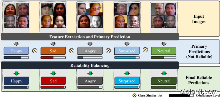
Fig. 1. A synopsis of ARBEx. Feature Extraction provides feature maps to generate initial predictions. Confidence distributions of initial labels are mostly inconsistent, unstable and unreliable. Reliability Balancing approach aids in stabilizing the distributions and addressing inconsistent and unreliable labeling.
图 1: ARBEx概要。特征提取模块提供特征图以生成初始预测。初始标签的置信度分布大多不一致、不稳定且不可靠。可靠性平衡方法有助于稳定分布并解决不一致和不可靠的标注问题。
However, despite its recent outstanding performance, FEL is still considered as a difficult task due to a few reasons: (1) Global information. Existing FEL methods fail to acknowledge global factors of input images due to the constraints of convolutional local receptive fields, (2) Interclass similarity. Several expression categories frequently include similar images with little differences between them, (3) Intra-class disparity. Images from the same expression category might differ significantly from one another. For example, complexion, gender, image background, and an individual’s age vary between instances, and (4) Sensitivity
然而,尽管近期表现优异,面部表情识别 (FEL) 仍被视为一项具有挑战性的任务,原因包括:(1) 全局信息。现有FEL方法受限于卷积局部感受野,难以捕捉输入图像的全局特征;(2) 类间相似性。部分表情类别常包含高度相似的图像样本;(3) 类内差异。同一表情类别的图像可能存在显著差异,例如肤色、性别、背景及个体年龄等因素造成的实例间差异;(4) 敏感性
ARBEX
ARBEX
of scales. Variations in image quality and resolution can often compromise the efficacy of deep learning networks when used without necessary precaution. Images from inthe-wild datasets and other FEL datasets come in a wide range of image sizes. Consequently, it is essential for FEL to provide consistent performance across scales [39].
尺度变化。在不采取必要预防措施的情况下,图像质量和分辨率的差异往往会损害深度学习网络的效能。来自野外数据集和其他FEL数据集的图像尺寸范围广泛。因此,FEL必须在不同尺度上保持一致的性能[39]。
In view of these difficulties and with the ascent of Transformers in the computer vision research field [3], numerous FEL techniques incorporated with Transformers have been developed which have achieved state-of-the-art (SOTA) results. Kim et al. [15] further developed Vision Transformer (ViT) to consolidate both global and local features so ViTs can be adjusted to FEL tasks. Furthermore, [39] addresses scale sensitivity. Transformer models with multi channelbased cross-attentive feature extraction such as POSTER [56] and $\mathrm{POSTER{++}}$ [29] tackle all of the aforementioned issues present in ${\mathrm{FEL}},$ which use mutli-level cross attention based network powered by ViT to extract features. This architecture has surpassed many existing works in terms of performance owing to the help of its cross-fusion function, multi-scale feature extraction, and landmark-to-image branching method. The downsides of this complex design is that it easily overfits, does not employ heavy augmentation methods, nor does it deal with the certain bias, uncertainty awareness, and poor distribution of labels; problems commonly recognized in facial expression classification.
鉴于这些困难以及Transformer在计算机视觉研究领域的崛起[3],许多结合Transformer的FEL技术被开发出来,并取得了最先进(SOTA)的结果。Kim等人[15]进一步开发了Vision Transformer (ViT)来整合全局和局部特征,使ViT能够适应FEL任务。此外,[39]解决了尺度敏感性问题。采用多通道交叉注意力特征提取的Transformer模型,如POSTER[56]和$\mathrm{POSTER{++}}$[29],解决了${\mathrm{FEL}}$中存在的所有上述问题,这些模型使用基于ViT的多级交叉注意力网络来提取特征。得益于其交叉融合功能、多尺度特征提取和地标到图像的分支方法,该架构在性能方面超越了许多现有工作。这种复杂设计的缺点是容易过拟合,没有采用大量的增强方法,也没有处理某些偏差、不确定性意识和标签分布不均的问题;这些都是面部表情分类中普遍认可的问题。
To challenge this issue, we provide a novel reliability balancing approach where we place anchor points of different classes in the embeddings learned from [29]. These anchors have fixed labels and are used to calculate how similar the embeddings are to each label. We also add multi-head selfattention for the embeddings to find crucial components with designated weights to increase model reliability and robustness. This approach results in improved label distribution of the expressions along with stable confidence score for proper labeling in unreliable labels. To address the quick over fitting of enormous multi-level feature extraction procedures, we introduce heavy data augmentation and a robust training batch selection method to mitigate the risk of over fitting.
为应对这一问题,我们提出了一种新颖的可靠性平衡方法:在基于[29]学习的嵌入空间中放置不同类别的锚点。这些锚点具有固定标签,用于计算嵌入向量与各标签的相似度。同时,我们为嵌入层引入多头自注意力机制(multi-head self-attention),通过指定权重识别关键成分,从而提升模型的可靠性与鲁棒性。该方法能改善表情标签的分布状态,并为不可靠标签提供稳定的置信度评分。针对多层特征提取过程中易出现的过拟合问题,我们采用强数据增强技术和鲁棒的训练批次选择方法以降低过拟合风险。
In summary, our method offers unbiased and evenly distributed data to the image encoder, resulting in accurate feature maps. These feature maps are then utilized for drawing predictions with the assistance of reliability balancing section, ensuring robust outcomes regardless of potential bias and unbalance in the data and labels.
总之,我们的方法为图像编码器提供无偏且均匀分布的数据,从而生成准确的特征图。随后,这些特征图在可靠性平衡模块的辅助下用于绘制预测结果,确保无论数据和标签存在何种潜在偏差或不平衡,都能获得稳健的输出。
1.1 Our Contributions
1.1 我们的贡献
Our contributions are summarized into four folds:
我们的贡献可总结为以下四点:
We propose a novel approach ARBEx, a novel framework consisting multi-level attention-based feature extraction with reliability balancing for robust FEL with extensive data preprocessing and refinement methods to fight against biased data and poor class distributions. We propose adaptive anchors in the embedding space and multi-head self-attention to increase reliability and robustness of the model by correcting erroneous labels, providing more accurate and richer supervision for training the deep FEL network. We combine relationships between anchors and weighted values from attention mechanism to stabilise class distributions for poor predictions mitigating the issues of similarity in different classes effectively.
我们提出了一种新颖方法ARBEx,这是一个包含多级基于注意力的特征提取与可靠性平衡的创新框架,旨在通过广泛的数据预处理和优化方法实现鲁棒的特征嵌入学习(FEL),以应对有偏数据和不良类别分布。我们在嵌入空间中引入自适应锚点,并采用多头自注意力机制,通过纠正错误标签来提升模型的可靠性和鲁棒性,为深度FEL网络训练提供更精确、更丰富的监督信号。通过结合锚点关系与注意力机制的加权值,我们稳定了不良预测的类别分布,有效缓解了不同类别间相似性带来的问题。
Our streamlined data pipeline ensures welldistributed quality input and output embeddings, utilizing the full power of the Window-based CrossAttention Vision Transformer providing robust feature maps to identify facial expressions in a confident manner. Empirically, our ARBEx method is rigorously evaluated on diverse in-the-wild FEL databases. Experimental outcomes exhibit that our method consistently surpasses most of the state-of-art FEL systems.
我们精简的数据管道确保了质量分布均匀的输入和输出嵌入,充分利用了基于窗口的交叉注意力视觉Transformer (Vision Transformer) 的强大能力,提供稳健的特征图以自信地识别面部表情。实验表明,我们的ARBEx方法在多种野外面部表情识别 (FEL) 数据库上进行了严格评估。实验结果表明,我们的方法始终优于大多数最先进的FEL系统。
2 RELATED WORKS
2 相关工作
In this section, we highlighted relevant works in FEL with respect to Transformers, uncertainty, and attention networks.
在本节中,我们重点介绍了与Transformer、不确定性及注意力网络相关的联邦边缘学习 (FEL) 相关工作。
2.1 Facial Expression Learning (FEL)
2.1 面部表情学习 (Facial Expression Learning, FEL)
Most classic works related to FEL are used in a extensive variety, mainly in the computer vision and psychological science domains. In simple words, FEL is the task of labeling the expressions based on a facial image which consists of three phases, namely facial detection, feature extraction, and expression recognition [42]. In recent times, FEL systems have been more efficient and optimized by deep learning based algorithms, where self-supervised feature extraction [50] has been introduced. To extract global and local features from detected face, Weng et al. [46] implement a multibranch network. Xue et al. [49] build a relation-aware localpatch representations using retention module to explore extensive relations on the manifold local features based on multi-head self-attention and Transformer frameworks. Recently, both Li et al. [23] and Wang et al. [41] suggest attention networks based on regions to extract disc rim i native features which outperform for robust pose and occlusionaware FEL.
与FEL相关的大多数经典作品应用广泛,主要集中在计算机视觉和心理科学领域。简而言之,FEL是基于面部图像标注表情的任务,包含三个阶段:面部检测、特征提取和表情识别 [42]。近年来,基于深度学习的算法使FEL系统更加高效和优化,其中引入了自监督特征提取 [50]。为了从检测到的面部提取全局和局部特征,Weng等人 [46] 实现了一个多分支网络。Xue等人 [49] 使用保留模块构建了关系感知的局部块表示,基于多头自注意力 (multi-head self-attention) 和Transformer框架探索流形局部特征的广泛关系。最近,Li等人 [23] 和Wang等人 [41] 都提出了基于区域的注意力网络,用于提取判别性特征,在鲁棒的姿态和遮挡感知FEL中表现优异。
2.2 Transformers in FEL
2.2 FEL中的Transformer
According to recent works [32], ViT [11] exhibits remarkable resilience against severe disruption and occlusion. To handle the shortcomings of FEL, such as poor quality samples, different backdrops and annotator’s various contexts, Li et al. [22] introduce Mask Vision Transformer (MVT) to provide a mask that can remove complicated backdrops and facial occlusion, as well as an adaptive relabeling mechanism to fix inaccurate labels in real-world FEL archives. Addressing the inadequate performance of Transformers in recognizing the subtlety of expression in videos, Liu et al. [25] develop a novel Expression Snippet Transformer (EST) which successfully models minuscule intra/inter snippet visual changes and effectively learns the long-range spatialtemporal relations. While Transformers have proven to perform well in FEL tasks, it still has vulnerabilities when dealing with multimodal $\left(2\mathrm{D}+3\mathrm{D}\right)$ ) datasets, as it needs more data. To combat this problem, Li et al. [21] create a resilient lightweight multimodal facial expression vision Transformer for multimodal FEL data. Hwang et al. [14] propose Neural Resizer, a method that helps Transformers by balancing the noisiness and imbalance through datadriven information compensation and down scaling. Zhang et al. [53] develop a Transformer-based multimodal information fusion architecture that utilizes dynamic multimodal features to fully leverage emotional knowledge from diverse viewpoints and static vision points.
根据近期研究[32],ViT[11]展现出对严重干扰和遮挡的卓越鲁棒性。针对FEL存在的样本质量差、背景多样及标注者语境差异等问题,Li等人[22]提出掩码视觉Transformer (MVT),通过生成掩码消除复杂背景与面部遮挡,并采用自适应重标注机制修正真实场景FEL档案中的错误标签。为解决Transformer在视频微表情识别中的性能局限,Liu等人[25]开发了新型表达式片段Transformer (EST),成功建模片段内/间的细微视觉变化,并有效学习长程时空关联。尽管Transformer在FEL任务中表现优异,其处理多模态$\left(2\mathrm{D}+3\mathrm{D}\right)$数据集时仍存在数据需求量大等缺陷。为此,Li等人[21]构建了轻量级多模态面部表情视觉Transformer。Hwang等人[14]提出Neural Resizer方法,通过数据驱动的信息补偿与降采样平衡噪声与不均衡问题。Zhang等人[53]设计了基于Transformer的多模态信息融合架构,利用动态多模态特征充分挖掘多视角与静态视觉点的情感知识。

Fig. 2. Pipeline of ARBEx. Heavy Augmentation is applied to the input images and Data Refinement method selects training batch with properly distributed classes for each epoch. Window-Based Cross-Attention ViT framework uses mutli-level feature extraction and integration to provide embeddings (Feature Vectors). Linear Reduction Layer reduces the feature vector size for fast modeling. MLP predicts the primary labels and Confidence is calculated from label distribution. Reliability balancing receives embeddings and processes in two ways. Firstly, it places anchors in the embedding space. It improves prediction probabilities by utilizing trainable anchors for searching similarities in embedding space. On the other way, Multi-head self-attention values are used to calculate label correction and confidence. Weighted Average of these two are used to calculate the final label correction. Using label correction, primary label distribution and confidence, final corrected label distribution is calculated, making the model more reliable.
图 2: ARBEx流程框架。对输入图像进行重度增强(Heavy Augmentation),数据精炼(Data Refinement)方法为每个训练周期选择类别分布适当的批次。基于窗口的交叉注意力ViT框架通过多级特征提取与整合生成嵌入向量(Feature Vectors),线性降维层(Linear Reduction Layer)压缩特征维度以加速建模。MLP层预测初始标签,并根据标签分布计算置信度。可靠性平衡模块通过双路径处理嵌入向量:一方面在嵌入空间放置可训练锚点,通过相似性搜索优化预测概率;另一方面利用多头自注意力值计算标签校正量与置信度。二者的加权平均结果用于最终标签校正,结合初始标签分布与置信度生成修正后的标签分布,从而提升模型可靠性。
2.3 Uncertainty in FEL
2.3 FEL中的不确定性
Uncertainties refer to mainly cryptic expressions, imprecise and conflicting annotations in FEL tasks. To eliminate uncertainty annotations, Fan et al. [13] introduce mid-level representation enhancement (MRE) and graph-embedded uncertainty suppressing (GUS). For performing both cleaning noisy annotations and classifying facial images, Viet et al. [18] introduce a multitasking network architecture and Wen et al. [44] implement center loss for applying intra-class compactness to extract disc rim i native features to reduce uncertain predictions. For determining facial expression with noisy annotations, Max-Feature-Map activation function is adopted by Wu et al. [47].
不确定性主要指FEL任务中的隐晦表达、不精确和冲突的标注。为消除不确定性标注,Fan等人[13]提出了中层表示增强(MRE)和基于图嵌入的不确定性抑制(GUS)。Viet等人[18]设计了多任务网络架构来同时清理噪声标注和分类面部图像,Wen等人[44]则采用中心损失函数通过类内紧致性提取判别性特征以减少不确定预测。针对带噪声标注的面部表情识别,Wu等人[47]采用了Max-Feature-Map激活函数。
2.4 Attention Networks in FEL
2.4 FEL中的注意力网络
Despite FEL gaining widespread recognition in the field of computer vision, two major problems- pose alterations and occlusion have not been properly addressed in terms of automatic expression detection. Wang et al. [40] develop a system where Facial Expression Recognition (FER) datasets are annotated to include pose and real-world occlusion features. They also preset a Region Attention Network to encapsulate face areas and poses in an adaptive manner. Furthermore, a region-based loss function is introduced to induce larger attention weights. Another work that deals with such issues is by Zhao et al. [54] where they propose a global multi-scale and local attention network (MA-Net) which consists of a multi-scale based local attention component with a feature pre-extractor that aids in focusing more on salient details. Inter-class similarity and models lacking high-order interactions among local aspects are some other problems present in current FER systems. Wen et al. present Distract your Attention Network (DAN) [45] with integral sections. They are Feature Clustering Network (FCN) which retrieves robust features by using a large-margin learning
尽管FEL(面部表情学习)在计算机视觉领域获得了广泛认可,但姿态变化和遮挡这两大问题在自动表情检测方面仍未得到妥善解决。Wang等人[40]开发了一个系统,对面部表情识别(FER)数据集进行标注以包含姿态和真实世界遮挡特征。他们还预设了一个区域注意力网络,以自适应方式封装面部区域和姿态。此外,引入基于区域的损失函数来产生更大的注意力权重。Zhao等人[54]的另一项工作也处理了此类问题,他们提出了一种全局多尺度和局部注意力网络(MA-Net),该网络包含基于多尺度的局部注意力组件和一个特征预提取器,有助于更关注显著细节。类间相似性和模型缺乏局部方面间高阶交互是当前FER系统中存在的其他问题。Wen等人提出了具有完整组件的分散注意力网络(DAN)[45],其中包括特征聚类网络(FCN),该网络通过使用大间隔学习来检索鲁棒特征。
ARBEX
ARBEX
goal, Multi-head cross Attention Network (MAN) initializes a variety of attention heads to focus on multiple facial features at the same time and develop attention maps on these areas, and Attention Fusion Network (AFN) which integrates multiple attention maps from various regions into a single, unified map. Fernandez et al. [30] propose Facial Expression Recognition with Attention Net (FERAtt) which utilizes Gaussian space representation to recognize facial expressions. The architecture focuses on facial image correction, which employs a convolutional-based feature extractor in combination with an encoder-decoder structure, and facial expression categorization, which is in charge of getting an embedded representation and defining the facial expression.
目标,多头交叉注意力网络 (MAN) 初始化多种注意力头以同时关注多个面部特征,并在这些区域生成注意力图;注意力融合网络 (AFN) 则将来自不同区域的多个注意力图整合为单一统一图。Fernandez 等人 [30] 提出了基于注意力网络的面部表情识别方法 (FERAtt),该方法利用高斯空间表示来识别面部表情。该架构专注于面部图像校正(采用基于卷积的特征提取器与编码器-解码器结构相结合)和面部表情分类(负责获取嵌入表示并定义面部表情)。
3 APPROACH
3 方法
In our comprehensive approach, we propose a rigorous feature extraction strategy that is supported by ViT with reliability balancing mechanism to tackle the difficulties of FEL. Its cutting-edge framework is composed of a variety of components that function together to provide solutions that are accurate and reliable. We start by scaling the input photos before initiating the augmentation procedure in order to achieve better augmentation. Following image scaling, there is rotation, color enhancement, and noise balancing. The images are then randomly cropped for the optimal outcomes after extensive augmentation. Our pipeline meticulously addresses different biases and over fitting possibilities that may exist in the training data by randomly selecting a few images from each video and assembling them. Furthermore, we randomly select a set of images representing each expression for every epoch. The overall selection process and the parameters varies on different datasets based on their distribution of labels, number of classes and images.
在我们的综合方法中,我们提出了一种严格的特征提取策略,该策略由具备可靠性平衡机制的ViT支持,以应对FEL的难题。其前沿框架由多种组件构成,这些组件协同工作以提供准确可靠的解决方案。我们首先对输入照片进行缩放,然后启动增强程序以获得更好的增强效果。图像缩放之后进行旋转、色彩增强和噪声平衡。经过大量增强后,图像会被随机裁剪以获得最佳结果。我们的流程通过从每个视频中随机选择少量图像并进行组合,细致地解决了训练数据中可能存在的不同偏差和过拟合问题。此外,我们在每个epoch随机选择一组代表每种表情的图像。整体选择过程和参数会根据不同数据集的标签分布、类别数量和图像数量而变化。
In our approach, the cross-attention ViT is used in the feature extraction process. Which is aimed at tackling common FEL issues, including scale sensitivity, intra-class discrepancy, as well as inter-class similarity. We employ a pre-trained landmark extractor to locate different facial landmarks on a particular face. Afterward, we use a pretrained image backbone model to extract features from the image accordingly. We utilize multiple feature extractors to detect low-level to high-level features in the image using different facial landmarks. After feature extraction, collected multi-level feature information is integrated. We use a cross-attention mechanism for linear computation and it integrates multi-level features and provides feature vector embedding using a optimised version of $\mathrm{POSTER{++}}$ [29]. This comprehensive feature extraction framework provides correctness and dependability in the final output vector of length 768 by combining a cross-attention mechanism with substantial feature extraction. We also use an additional linear reduction layer to decrease the feature vector size to 128. Primary label distributions are generated using logits resulted by Multi-Layer Perce ptr on s. Multi-Layer Perceptrons (MLP) include variety of hidden layers that enable them to process information with great precision and accuracy. We calculated confidence value based on the primary label distribution using Normalized Entropy to evaluate the reliability [17] of these models.
在我们的方法中,特征提取过程采用了交叉注意力视觉Transformer (ViT)。该方法旨在解决常见的面部表情识别(FEL)问题,包括尺度敏感性、类内差异以及类间相似性。我们使用预训练的关键点检测器定位特定面部的不同面部特征点,随后通过预训练的图像主干模型提取相应图像特征。利用多级特征提取器,基于不同面部关键点检测从低层到高层的图像特征。
特征提取完成后,将收集的多层级特征信息进行整合。采用交叉注意力机制进行线性计算,该机制整合多层级特征并通过优化版$\mathrm{POSTER{++}}$[29]生成特征向量嵌入。这一综合特征提取框架结合交叉注意力机制与多层次特征提取,最终输出长度为768的向量,确保其正确性与可靠性。我们还额外使用线性降维层将特征向量尺寸缩减至128。
通过多层感知器(MLP)输出的logits生成初始标签分布。MLP包含多种隐藏层,使其能够以高精度处理信息。基于初始标签分布,我们采用归一化熵计算置信度值,以评估这些模型的可靠性[17]。
We introduce a novel reliability balancing method to solve the limitations of modern FEL models. Modern FEL models still have several limitations, especially when it comes to making precise predictions for classes because their images are quite similar. This issue leads to a biased and unreliable model. Our reliability balancing method can increase the prediction capability of unbalanced and erroneous predictions, thereby improving the performance of the model. We achieve enhanced reliability and confidence by placing multiple learnable anchors in the embedding space and using multi-head self- attention mechanism, which help identify the closest neighbors of erroneous predictions to improve the prediction ability. The use of anchor spaces and attention values have proven to be highly effective in stabilizing label distribution, thereby resulting in better performance overall. We obtain additional regular iz ation whenever possible by implementing dropout layers for more robustness. Our approach ensures that the model is resilient even in the circumstance of noisy or inadequate data; minimizing possible bias and over fitting. The resulting model integrating extensive feature extraction with reliability balancing, is remarkably precise and able to make credible predictions even in the context of ambiguity. The overall pipeline is illustrated in Fig. 2.
我们提出了一种新颖的可靠性平衡方法,以解决现代FEL模型的局限性。现代FEL模型仍存在若干不足,特别是在对图像高度相似的类别进行精确预测时,这一问题会导致模型出现偏差且不可靠。我们的可靠性平衡方法能够提升对不平衡和错误预测的判定能力,从而改善模型性能。通过在嵌入空间放置多个可学习锚点并采用多头自注意力机制,我们实现了更高的可靠性和置信度——该机制能识别错误预测的最近邻以提升预测能力。实践证明,锚点空间和注意力值能有效稳定标签分布,从而全面提升性能。我们还尽可能通过实现dropout层来获得额外正则化,以增强鲁棒性。该方法确保模型即使在噪声或数据不足的情况下仍具韧性,最大限度减少潜在偏差和过拟合。最终模型将广泛特征提取与可靠性平衡相结合,展现出卓越的精确性,即使在模糊情境下也能做出可信预测。整体流程如图2所示。
3.1 Problem Formulation
3.1 问题表述
Let $x^{i}$ be the $i$ -th instance variable in the input space $\mathcal{X}$ and $y^{i}\in\mathcal{V}$ be the label of the $i$ -th instance with $Y={y_{1},y_{2} y_{N}}$ being the label set. Let $\mathcal{P}^{n}$ be the set of all probability vectors of size $n$ . Furthermore, let $l^{i}\in\mathcal{P}^{N}$ be the discrete label distribution of $i$ -th instance. Additionally, let $e=p(x;\theta_{p})$ be the embedding output of the WindowBased Cross-Attention ViT (explained in 3.2) network $p$ with parameters $\theta_{p}$ and let $f(e;\theta_{f})$ be the logit output of the MLP classification head network $f$ with parameters $\theta_{f}$ .
设 $x^{i}$ 为输入空间 $\mathcal{X}$ 中的第 $i$ 个实例变量,$y^{i}\in\mathcal{V}$ 为第 $i$ 个实例的标签,其中 $Y={y_{1},y_{2} y_{N}}$ 为标签集。令 $\mathcal{P}^{n}$ 表示所有大小为 $n$ 的概率向量集合。此外,设 $l^{i}\in\mathcal{P}^{N}$ 为第 $i$ 个实例的离散标签分布。另设 $e=p(x;\theta_{p})$ 为基于窗口交叉注意力 ViT (详见 3.2 节) 网络 $p$ 的嵌入输出,其参数为 $\theta_{p}$;$f(e;\theta_{f})$ 为 MLP 分类头网络 $f$ 的逻辑输出,其参数为 $\theta_{f}$。
3.2 Window-Based Cross-Attention ViT
3.2 基于窗口的交叉注意力 ViT
We use a complex image encoder to capture distinctive patterns from the input images. We obtain feature embedding vectors in our proposed pipeline with a refined and optimised version of POSTER $^{++}$ [29], a window-based cross-attention ViT network.
我们采用复杂的图像编码器从输入图像中捕捉独特模式。通过改进优化版的POSTER$^{++}$[29](一种基于窗口交叉注意力机制的ViT网络),在提出的流程中获取特征嵌入向量。
We employ a window-based cross-attention mechanism to achieve linear computation. We extract features by the image backbone and facial landmark detectors. We used IR50 [43] as image backbone and Mobile Face Net [6] as facial landmark detector. For each level, firstly, division of image features $X_{i m g}\in\mathcal{R}^{N\times D}$ is performed, where $N$ represents the number of classes and $D$ denotes the feature dimensions. These divided image features are transformed into many non-overlapping windows, $z_{i m g}\in\mathcal{R}^{M\times D}$ where $z_{i m g}$ contains $M$ tokens. Then, down-sampling of the landmark feature Xlm ∈ RC×H×W t akes place, where $C$ is the number of channels in the attention network, $H$ and $W$ are the height and width of the image. The downsampled features are converted into the window size, where the smaller representation of the image is taken and it is represented by $z_{l m}\in\mathcal{R}^{c\times h\times w}$ where $c=D,h\times w=\mathbf{M}$ . The features are reshaped in accordance with $z_{i m g}$ ’s shape.
我们采用基于窗口的交叉注意力机制来实现线性计算。通过图像主干网络和人脸关键点检测器提取特征,其中图像主干网络采用IR50 [43],人脸关键点检测器采用Mobile Face Net [6]。对于每个层级,首先对图像特征$X_{img}\in\mathcal{R}^{N\times D}$进行划分,其中$N$表示类别数量,$D$表示特征维度。这些划分后的图像特征被转换为多个不重叠的窗口$z_{img}\in\mathcal{R}^{M\times D}$,其中$z_{img}$包含$M$个token。接着对关键点特征$X_{lm}\in\mathcal{R}^{C\times H\times W}$进行下采样,其中$C$是注意力网络的通道数,$H$和$W$是图像的高度和宽度。下采样后的特征被转换为窗口尺寸,此时取图像的较小表示形式,记为$z_{lm}\in\mathcal{R}^{c\times h\times w}$,其中$c=D$,$h\times w=\mathbf{M}$。最终将这些特征按照$z_{img}$的形状进行重塑。
ARBEX
ARBEX
The cross-attention with $I$ heads in a local window can be formulated as follows at this point:
此时,局部窗口中具有 $I$ 个头的交叉注意力可表述如下:
$$
\begin{array}{c}{{q=z_{l m}w_{q},k=z_{i m g}w_{k},v=z_{i m g}w_{v}}}\ {{\mathrm{}_{o}(\mathrm{\ensuremath{^{(i)}}}=s o f t m a x(q^{(i)}k^{(i)T}/\sqrt{d}+b)v^{(i)},i=1,...,I}}\ {{\mathrm{}_{o}=[o^{(1)},...,o^{(I)}]w_{o}}}\end{array}
$$
$$
\begin{array}{c}{{q=z_{l m}w_{q},k=z_{i m g}w_{k},v=z_{i m g}w_{v}}}\ {{\mathrm{}_{o}(\mathrm{\ensuremath{^{(i)}}}=s o f t m a x(q^{(i)}k^{(i)T}/\sqrt{d}+b)v^{(i)},i=1,...,I}}\ {{\mathrm{}_{o}=[o^{(1)},...,o^{(I)}]w_{o}}}\end{array}
$$
where $w_{q},~w_{k},~w_{v}$ and $w_{o}$ are the matrices used for mapping the landmark-to-image features, and $\ensuremath{\boldsymbol{q}},\ensuremath{\boldsymbol{k}},\ensuremath{\boldsymbol{v}}$ denote the query matrix for landmark stream, and key, and value matrices for the image stream, respectively from different windows used in the window-based attention mechanism. [·] represents the merge operation where the images patches are combined to identify the correlations between them and lastly, the relative position bias is expressed as $b\in\mathcal{R}^{I\times I}$ which aids in predicting the placement between landmarks and image sectors.
其中 $w_{q},~w_{k},~w_{v}$ 和 $w_{o}$ 是用于映射地标到图像特征的矩阵,$\ensuremath{\boldsymbol{q}},\ensuremath{\boldsymbol{k}},\ensuremath{\boldsymbol{v}}$ 分别表示地标流的查询矩阵、图像流的键矩阵和值矩阵,这些矩阵来自基于窗口的注意力机制中使用的不同窗口。[·] 表示合并操作,其中图像块被组合以识别它们之间的相关性,最后,相对位置偏置表示为 $b\in\mathcal{R}^{I\times I}$,有助于预测地标和图像区域之间的位置关系。[20]
We use the equations above for calculating the crossattention for all the windows. This method is denoted as Window-based Multi-head CrosS-Attention (W-MCSA). Using the equations below, the Transformer encoder for the cross-fusion can be calculated as:
我们使用上述方程计算所有窗口的交叉注意力。该方法称为基于窗口的多头交叉注意力 (W-MCSA)。利用以下方程,可以计算出用于交叉融合的Transformer编码器:
$$
X_{i m g}^{\prime}=W\ –M C S A_{(i m g)}+X_{i m g}
$$
$$
X_{i m g}^{\prime}=W\ –M C S A_{(i m g)}+X_{i m g}
$$
$$
X_{i m g_O}=M L P(N o r m(X_{i m g}^{\prime}))+X_{i m g}^{\prime}
$$
$$
X_{i m g_O}=M L P(N o r m(X_{i m g}^{\prime}))+X_{i m g}^{\prime}
$$
where $X_{i m g}^{\prime}$ is the combined image feature using WMCSA, $X_{i m g_O}$ the output of the Transformer encoder, and $N o r m(\cdot)$ represents a normalization operation for the full image of all windows combined. Using window information and dimensions $(z_{i m g},M,D,C,H,W,e t c.).$ , we extract and combine window based feature information to $X o_{i}$ $\mathrm{(\it\Omega_{i})}$ -th level window-based combined features of each image) from $X_{i m g_O}$ (extracted features of all windows of each image together).
其中 $X_{i m g}^{\prime}$ 是使用 WMCSA 的组合图像特征,$X_{i m g_O}$ 是 Transformer 编码器的输出,$N o r m(\cdot)$ 表示对所有窗口组合后的完整图像进行归一化操作。利用窗口信息和维度 $(z_{i m g},M,D,C,H,W,e t c.)$,我们从 $X_{i m g_O}$(每张图像所有窗口的提取特征集合)中提取并组合基于窗口的特征信息,得到 $X o_{i}$(每张图像第 $\mathrm{(\it\Omega_{i})}$ 级基于窗口的组合特征)。
We introduce a Vision Transformer to integrate the obtained features at multiple scales $X o_{1},...,X o_{i}$ . Our attention mechanism is able to capture long-range dependencies as it combines information tokens of all scale feature maps like POSTER $^{++}$ [29]. The method is described as:
我们引入了一个Vision Transformer来整合多尺度下获取的特征$X o_{1},...,X o_{i}$。我们的注意力机制能够捕捉长距离依赖关系,因为它像POSTER$^{++}$[29]一样结合了所有尺度特征图的信息Token。该方法描述如下:
$$
X o=[X o_{1},...,X o_{i}]
$$
$$
X o=[X o_{1},...,X o_{i}]
$$
$$
X o^{\prime}=M H S A(X o)+X o
$$
$$
X o^{\prime}=M H S A(X o)+X o
$$
$$
X o_{o u t}=M L P(N o r m(X o))+X o^{'}
$$
$$
X o_{o u t}=M L P(N o r m(X o))+X o^{'}
$$
where, $\left[\cdot\right]$ denotes concatenation, $M H S A(\cdot)$ denotes multihead self-attention mechanism, $M L P(\cdot)$ is the multi-layer perceptron.
其中,$\left[\cdot\right]$ 表示拼接操作,$M H S A(\cdot)$ 表示多头自注意力机制,$M L P(\cdot)$ 为多层感知机。
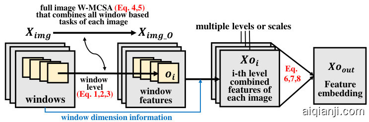
Fig. 3. Data flow in the Window-Based Cross-Attention ViT network
图 3: 基于窗口交叉注意力ViT网络的数据流
Output of the multi-scale feature combination module $X o_{o u t},$ which is equal to feature embedding $e,$ is the final output of the encoder network denoted by $p(x;\theta_{p})$ .
多尺度特征组合模块的输出 $X o_{o u t},$ 即特征嵌入 $e,$ 是编码器网络 $p(x;\theta_{p})$ 的最终输出。
3.3 Reliability Balancing
3.3 可靠性平衡
Majority of Facial Expression Learning datasets are labeled using only one label for each sample. Inspired by [10], [17], we provide an alternative approach, in which, we learn and improve label distributions utilizing a label correction approach. We calculate a label distribution primarily that uses the embedding $e$ directly into the MLP network. Subsequently, the reliability balancing section employs label correction techniques to stabilize the primary distribution. This results in improved predictive performance through more accurate and reliable labeling.
大多数面部表情学习数据集每个样本仅使用一个标签进行标注。受 [10]、[17] 启发,我们提出了一种替代方法:通过标签校正技术学习并优化标签分布。首先,我们利用嵌入 $e$ 直接输入 MLP 网络计算初始标签分布,随后通过可靠性平衡模块运用标签校正技术来稳定初始分布。这种方法通过更精确可靠的标注提升了预测性能。
Primary Label Distribution. From sample $x,$ using the $p$ network we can generate the corresponding embedding $\boldsymbol{e}~=~p(\boldsymbol{x};\boldsymbol{\theta}_{p})$ and using the $f$ -network consisting MLP, we can generate the corresponding discrete primary label distribution:
主标签分布。从样本$x$出发,利用$p$网络生成对应的嵌入$\boldsymbol{e}~=~p(\boldsymbol{x};\boldsymbol{\theta}_{p})$,再通过包含MLP的$f$网络生成对应的离散主标签分布:
$$
l=s o f t m a x(f(e;\theta_{f}))
$$
$$
l=s o f t m a x(f(e;\theta_{f}))
$$
We use the information contained in the label distribution with label corrections during training to improve the model performance.
我们利用训练过程中带有标签校正的标签分布信息来提升模型性能。
Confidence Function. To evaluate the credibility of predicted probabilities, a confidence function is designed. Let $C:{\mathcal{P}}^{\hat{N}}\rightarrow[0,1].$ , be the confidence function. $C$ measures the certainty of a prediction made by the classifier using normalized entropy function $\mathrm{H}(1)$ . The functions are defined as:
置信函数 (Confidence Function)。为了评估预测概率的可信度,设计了一个置信函数。令 $C:{\mathcal{P}}^{\hat{N}}\rightarrow[0,1].$ 为置信函数。$C$ 通过归一化熵函数 $\mathrm{H}(1)$ 来衡量分类器预测的确定性。函数定义如下:
$$
C(l)=1-H(l)
$$
$$
C(l)=1-H(l)
$$
$$
H(l)=-\frac{\sum_{i}l^{i}\log(l^{i})}{N}
$$
$$
H(l)=-\frac{\sum_{i}l^{i}\log(l^{i})}{N}
$$
For a distribution where all probabilities are equal; normalized entropy is 1, and confidence value is 0. Where one value is equal to 1, and others are equal to $0_{,}$ ; normalized entropy is 0, and confidence value is 1.
对于一个所有概率均等的分布,归一化熵为1,置信度值为0。当某个值等于1而其余值等于$0_{,}$时,归一化熵为0,置信度值为1。
3.4 Label Correction
3.4 标签校正
The conundrum of label accuracy, distribution stability, and reliability has been a mainstream problem in FEL. The novel approach we propose to resolve this is a combination of two distinct measures of label correction: Anchor Label Correction and Attentive Correction. By leveraging geometric similarities and state-of-the-art multi-head attention mechanism, we are designing predicted labels are not only accurate but also stable and reliable.
标签准确性、分布稳定性和可靠性的困境一直是FEL领域的主流难题。我们提出的创新解决方案结合了两种不同的标签校正方法:锚定标签校正 (Anchor Label Correction) 和注意力校正 (Attentive Correction) 。通过利用几何相似性和最先进的多头注意力机制 (multi-head attention mechanism) ,我们设计的预测标签不仅准确,而且稳定可靠。
3.4.1 Anchor Label Correction
3.4.1 锚点标签校正
Anchor Notations. We define anchor $a^{i,j}\quad(i\quad\in$ ${1,2...,N},j\in{1,2...K})$ to be a point in the embedding space. Let $\mathcal{A}$ be a set of all anchors. During training we use $K$ trainable anchors for each label, with $K$ being a hyper parameter. We assign another label distribution $m^{\check{i},j}\in\dot{\mathcal{P}}^{N}$ to anchor $a^{i,j}$ , where $m^{i,j}$ is defined as:
锚点表示法。我们将锚点 $a^{i,j}\quad(i\quad\in$ ${1,2...,N},j\in{1,2...K})$ 定义为嵌入空间中的一个点。设 $\mathcal{A}$ 为所有锚点的集合。训练时,我们为每个标签使用 $K$ 个可训练的锚点,其中 $K$ 是一个超参数。我们为锚点 $a^{i,j}$ 分配另一个标签分布 $m^{\check{i},j}\in\dot{\mathcal{P}}^{N}$ ,其中 $m^{i,j}$ 定义为:
$$
m_{k}^{i,j}=\left{{1,{\mathrm{ if~}}k=i}\atop{0,{\mathrm{~otherwise}}}\right.
$$
$$
m_{k}^{i,j}=\left{{1,{\mathrm{ if~}}k=i}\atop{0,{\mathrm{~otherwise}}}\right.
$$
ARBEX
ARBEX
Intuitively, here it means anchors $a^{1,1},a^{1,2}\dots a^{1,K}$ are labeled as belonging to class 1, anchors $a^{2,1},a^{2,2}\dots a^{2,K}$ are labeled as belonging to class 2 and so on.
直观地说,这意味着锚点 $a^{1,1},a^{1,2}\dots a^{1,K}$ 被标记为属于类别 1,锚点 $a^{2,1},a^{2,2}\dots a^{2,K}$ 被标记为属于类别 2,以此类推。
Geometric Distances and Similarities. To correct the final label and stabilize the distribution we use the geometric information about similarity between the embeddings and a fixed number of learnable points in the embedding space called anchors.
几何距离与相似性。为了修正最终标签并稳定分布,我们利用了嵌入向量与嵌入空间中一组固定数量的可学习点(称为锚点)之间的几何相似性信息。
The similarity score $s^{i j}(e)$ is a normalized measure of similarity between an embedding $x$ and an anchor $a^{i j}\in{\mathcal{A}}$ .
相似度分数 $s^{i j}(e)$ 是嵌入向量 $x$ 与锚点 $a^{i j}\in{\mathcal{A}}$ 之间相似性的归一化度量。
The distance between embedding $e$ and anchor $a$ for each batch and class is defined as:
嵌入向量 $e$ 与锚点 $a$ 在每批次和类别间的距离定义为:
Correction. To additionally correct and stabilize the label distributions, we use attention-based similarity function. The embedding $x$ is passed through the multi-head selfattention layer to obtain attentive correction term $t_{a}$ . General formula:
修正。为了进一步校正并稳定标签分布,我们采用基于注意力机制的相似度函数。将嵌入向量 $x$ 通过多头自注意力层,得到注意力校正项 $t_{a}$。通用公式为:
$$
t_{a}=s o f t m a x(W_{o u t})
$$
$$
t_{a}=s o f t m a x(W_{o u t})
$$
$t_{a}$ is reshaped as required.
$t_{a}$ 会根据需要重塑形状。
3.4.3 Final Label correction
3.4.3 最终标签校正
To combine the correction terms, we use weighted $\mathtt{s u m,}$ with weighting being controlled by the confidence of label corrections.
为了合并修正项,我们使用加权 $\mathtt{s u m}$,其权重由标签修正的置信度控制。
$$
d(e,a)=\sqrt{\sum_{d i m_{e}}|a-e|^{2}}
$$
$$
d(e,a)=\sqrt{\sum_{d i m_{e}}|a-e|^{2}}
$$
Here, $d i m_{e}$ is the dimension of embedding $e$ . Distances $|a-e|^{2}$ are reduced over the last dimension $d i m_{e}$ and element–wise square root is taken for stabilizing values.
这里,$d i m_{e}$ 是嵌入 $e$ 的维度。距离 $|a-e|^{2}$ 在最后一个维度 $d i m_{e}$ 上缩减,并对元素取平方根以稳定数值。
The similarity score $s^{i j}$ is then obtained by normalizing distances as softmax:
相似度分数 $s^{i j}$ 通过将距离归一化为 softmax 得到:
$$
s^{i j}(e)=\frac{\exp(-\frac{d(e,a^{i j})}{\delta})}{\sum_{i}^{N}\sum_{j}^{K}\exp(-\frac{d(e,a^{i j})}{\delta})}
$$
$$
s^{i j}(e)=\frac{\exp(-\frac{d(e,a^{i j})}{\delta})}{\sum_{i}^{N}\sum_{j}^{K}\exp(-\frac{d(e,a^{i j})}{\delta})}
$$
where, $\delta$ is a hyper parameter, which is used in the computation of softmax to control the steepness of the function. The default value used for $\delta$ is 1.0.
其中,$\delta$ 是一个超参数,用于计算 softmax 时控制函数的陡峭程度。$\delta$ 的默认值为 1.0。
Correction. From similarity scores we can calculate the anchor label correction term as follows:
修正。根据相似度分数,我们可以按如下方式计算锚点标签修正项:
$$
t_{g}(e)=\sum_{i}^{N}\sum_{j}^{K}s^{i j}(e)m^{i j}
$$
$$
t_{g}(e)=\sum_{i}^{N}\sum_{j}^{K}s^{i j}(e)m^{i j}
$$
3.4.2 Attentive Correction
3.4.2 注意力修正
Multi-head Self-Attention. For multi-head attention [38], Let a query with query embeddings $q\in\mathcal{R}^{d_{Q}}.$ , key embeddings $\dot{k}\in\dot{\mathcal{R}}^{d_{K}},$ , and value embeddings $v\in\mathcal{R}^{d_{V}}$ is given. With the aid of independently learned projections, they can be modified with $h,$ which is the attention head. These parameters are then supplied to attention pooling. Finally, these outputs are altered and integrated using another linear projection. The process is described as follows:
多头自注意力 (Multi-head Self-Attention)。对于多头注意力 [38],给定一个具有查询嵌入 $q\in\mathcal{R}^{d_{Q}}$ 、键嵌入 $\dot{k}\in\dot{\mathcal{R}}^{d_{K}},$ 和值嵌入 $v\in\mathcal{R}^{d_{V}}$ 的查询。借助独立学习的投影,它们可以用注意力头 $h$ 进行修改。然后这些参数被提供给注意力池化 (attention pooling)。最后,这些输出通过另一个线性投影进行变换和整合。该过程描述如下:
$$
t={\frac{c_{g}}{c_{g}+c_{a}}}t_{g}+{\frac{c_{a}}{c_{g}+c_{a}}}t_{a}
$$
$$
t={\frac{c_{g}}{c_{g}+c_{a}}}t_{g}+{\frac{c_{a}}{c_{g}+c_{a}}}t_{a}
$$
where $c_{g}=C(t_{g})$ and $c_{a}=C(t_{a})$ .
其中 $c_{g}=C(t_{g})$ 和 $c_{a}=C(t_{a})$ 。
Finally, to obtain the final label distribution $L_{f i n a l},$ we use a weighted sum of label distribution $l$ and label correction $t$ .
最后,为了获得最终的标签分布 $L_{f i n a l},$ 我们使用标签分布 $l$ 和标签校正 $t$ 的加权求和。
$$
L_{f i n a l}=\frac{c_{l}}{c_{l}+c_{t}}l+\frac{c_{t}}{c_{l}+c_{t}}t
$$
$$
L_{f i n a l}=\frac{c_{l}}{c_{l}+c_{t}}l+\frac{c_{t}}{c_{l}+c_{t}}t
$$
where $c_{l}=C(l)$ and $c_{t}=C(t)$ .
其中 $c_{l}=C(l)$ 和 $c_{t}=C(t)$。
The label with maximum value in final corrected label distribution $L_{f i n a l}$ is provided as corrected label or final predicted label.
最终修正标签分布$L_{final}$中值最大的标签将作为修正标签或最终预测标签提供。
3.5 Loss Function
3.5 损失函数
Loss function used to train the model consists of three terms such as class distribution loss, anchor loss, and center loss.
用于训练模型的损失函数包含三个部分:类别分布损失 (class distribution loss)、锚点损失 (anchor loss) 和中心损失 (center loss)。
Class Distribution Loss $(\mathcal{L}_{c l s})$ : To make sure each example is classified correctly, we use the negative log-likelihood loss between the corrected label distribution $L^{i}$ and label $y^{i}$ :
类别分布损失 $(\mathcal{L}_{c l s})$ : 为确保每个样本被正确分类,我们使用修正后的标签分布 $L^{i}$ 与真实标签 $y^{i}$ 之间的负对数似然损失:
$$
\mathcal{L}{c l s}=-\sum_{i}^{m}\sum_{j}^{N}y_{j}^{i}\log L_{j}^{i}
$$
$$
\mathcal{L}{c l s}=-\sum_{i}^{m}\sum_{j}^{N}y_{j}^{i}\log L_{j}^{i}
$$
Anchor Loss $(\mathcal{L}_{a})$ ): In order to amplify the discriminatory capacity of the model, we want to make margins between anchors large so that we add an additional loss term:
锚点损失 $(\mathcal{L}_{a})$ ):为了增强模型的判别能力,我们希望扩大锚点之间的间隔,因此引入额外的损失项:
$$
h_{i}=f(W_{i}^{(q)}q,W_{i}^{(k)}k,W_{i}^{(v)}v)\in\mathcal{R}^{p_{V}},
$$
$$
h_{i}=f(W_{i}^{(q)}q,W_{i}^{(k)}k,W_{i}^{(v)}v)\in\mathcal{R}^{p_{V}},
$$
$$
\mathcal{L}{a}=-\sum_{i}\sum_{j}\sum_{k}\sum_{l}|a^{i j}-a^{k l}|_{2}^{2}
$$
$$
\mathcal{L}{a}=-\sum_{i}\sum_{j}\sum_{k}\sum_{l}|a^{i j}-a^{k l}|_{2}^{2}
$$
where W i(Q) $\begin{array}{c c c c c c}{W_{i}^{(Q)}}&{\in}&{{\mathcal{R}}^{d_{Q}\times p_{Q}},W_{i}^{(K)}}&{\in}&{{\mathcal{R}}^{d_{K}\times p_{K}},W_{i}^{(V)}}&{\in}\end{array}$ ${\mathcal{R}}^{d_{V}\times p_{V}}$ are trainable parameters, and $f$ is the attentive pooling and $h_{i}(i=1,2,...,n_{h e a d s})$ is the attention head. The output obtained through learnable features, $W_{o u t}\in$ $\mathcal{R}^{p_{o u t}\times h\dot{p}_{o u t}}$ can be categorized as:
其中 $W_{i}^{(Q)}$ $\begin{array}{c c c c c c}{W_{i}^{(Q)}}&{\in}&{{\mathcal{R}}^{d_{Q}\times p_{Q}},W_{i}^{(K)}}&{\in}&{{\mathcal{R}}^{d_{K}\times p_{K}},W_{i}^{(V)}}&{\in}\end{array}$ ${\mathcal{R}}^{d_{V}\times p_{V}}$ 是可训练参数,$f$ 是注意力池化操作,$h_{i}(i=1,2,...,n_{heads})$ 是注意力头。通过可学习特征 $W_{out}\in$ $\mathcal{R}^{p_{out}\times h\dot{p}_{out}}$ 获得的输出可分类为:
We include the negative term in front because we want to maximize this loss. The loss is also normalized for standard uses.
我们在前面加入负号是因为我们希望最大化这个损失。该损失也针对标准用途进行了归一化处理。
Center Loss $(\mathcal{L}_{c})$ : To make anchors good representation of their class, we want to make sure anchors and embeddings of the same class stay close in the embedding space. To ensure that, we add an additional error term:
中心损失 $(\mathcal{L}_{c})$ : 为了使锚点能够良好地表征其类别,我们希望确保同一类别的锚点和嵌入在嵌入空间中保持接近。为此,我们添加了一个额外的误差项:
$$
W_{o u t}\left[\begin{array}{c}{h_{1}}\ {\vdots}\ {h_{n_{h e a d s}}}\end{array}\right]\in\mathcal{R}^{p_{o u t}}
$$
$$
W_{o u t}\left[\begin{array}{c}{h_{1}}\ {\vdots}\ {h_{n_{h e a d s}}}\end{array}\right]\in\mathcal{R}^{p_{o u t}}
$$
As we are using self-attention, all inputs $(q,k,v$ denoting query, key and value parameters respectively) are equal to the embedding $e$ .
由于我们使用的是自注意力机制 (self-attention),所有输入 $(q,k,v$ 分别表示查询、键和值参数) 都等于嵌入 $e$。
$$
\mathcal{L}{c}=\operatorname*{min}{k}|x^{i}-a^{y^{i}k}|_{2}^{2}
$$
$$
\mathcal{L}{c}=\operatorname*{min}{k}|x^{i}-a^{y^{i}k}|_{2}^{2}
$$
Total Loss $(\mathcal{L}_{t o t a l})$ ): Our final loss function can be defined as:
总损失 $(\mathcal{L}_{t o t a l})$ ): 我们的最终损失函数可定义为:
$$
\mathcal{L}{t o t a l}=\lambda_{c l s}\mathcal{L}{c l s}+\lambda_{a}\mathcal{L}{a}+\lambda_{c}\mathcal{L}_{c}
$$
$$
\mathcal{L}{t o t a l}=\lambda_{c l s}\mathcal{L}{c l s}+\lambda_{a}\mathcal{L}{a}+\lambda_{c}\mathcal{L}_{c}
$$
with $\lambda_{c l s},\lambda_{a},\lambda_{c}$ being hyper parameters, used to keep the loss functions in same scale.
其中 $\lambda_{c l s}$、$\lambda_{a}$、$\lambda_{c}$ 为超参数,用于保持损失函数在同一量级。
ARBEX
ARBEX
4 EXPERIMENTS
4 实验
4.1 Datasets
4.1 数据集
Aff-Wild2 [16] has 600 annotated audiovisual videos with 3 million frames for categorical and dimensional affect and action units models. It has 546 videos for expression recognition, with 2.6 million frames and 437 subjects. Experts annotated it frame-by-frame for six distinct expressions - surprise, happiness, anger, disgust, fear, neutral expression, and ’other’ emotional states.
Aff-Wild2 [16] 包含600个带标注的视听视频,共计300万帧,用于分类和维度情感及动作单元模型。其中546个视频用于表情识别,包含260万帧和437名受试者。专家逐帧标注了六种基本表情(惊讶、快乐、愤怒、厌恶、恐惧、中性)以及"其他"情绪状态。
RAF-DB [19], [20] contains a whopping 30,000 distinct images that encompass 7 unique labels for expressions. The images have been meticulously labeled by 40 individual annotators and boast a diverse range of attributes, including subsets of emotions, landmark locations, bounding boxes, race, age range, and gender attributions.
RAF-DB [19], [20] 包含高达30,000张不同的图像,涵盖7种独特的表情标签。这些图像由40位独立标注者精心标注,并拥有多样化的属性,包括情感子集、关键点位置、边界框、种族、年龄范围和性别属性。
JAFFE [27], [28] dataset comprises facial expressions from ten Japanese women, featuring seven prearranged expressions and multiple images for each individual depicting the respective expressions. The dataset encompasses a total of 213 images, with each image rated on six facial expressions by 60 Japanese viewers. The images are stored in an uncompressed 8-bit grayscale TIFF format, exhibit a resolution of $256\times256$ pixels, and contain no compression.
JAFFE [27], [28] 数据集包含十位日本女性的面部表情,涵盖七种预设表情及每位个体对应表情的多张图像。该数据集共计213张图像,每张图片由60位日本观察者对六种面部表情进行评分。图像以未压缩的8位灰度TIFF格式存储,分辨率为 $256\times256$ 像素,且无压缩处理。
FERG-DB [1] database is yet another benchmark repository that features 2D images of six distinct, stylized personages that were produced and rendered using the sophisticated MAYA software. Comprising an impressive quota of 55,767 meticulously annotated facial expression images, this mammoth database is categorized into seven distinct emotion classes: disgust, surprise, sadness, fear, joy, neutral, and anger.
FERG-DB [1] 数据库是另一个基准存储库,其特色是使用精密的MAYA软件制作并渲染的六种独特风格化角色的2D图像。该庞大数据库包含55,767张精心标注的面部表情图像,分为七种不同的情绪类别:厌恶、惊讶、悲伤、恐惧、快乐、中立和愤怒。
$\mathbf{FER}+$ [2] annotations have bestowed a novel set of labels upon the conventional Emotion FER dataset. Each image in $\mathrm{FER+}$ has undergone rigorous scrutiny from a pool of 10 taggers, thereby generating high-quality ground truths for still-image emotions that surpass the original FER labels. It contains seven main labels and one for exclusions.
$\mathbf{FER}+$ [2] 标注为传统情感识别数据集 FER 赋予了一套全新的标签体系。$\mathrm{FER+}$ 中的每张图像都经过10名标注员的严格审核,从而为静态图像情感生成了超越原始FER标签的高质量基准真值。该数据集包含七种主要情感标签和一种排除类别标签。

Fig. 4. Examples of training samples in different datasets
图 4: 不同数据集中的训练样本示例
4.2 Data Distribution Adjustments
4.2 数据分布调整
4.2.1 Augmentation
4.2.1 数据增强
Sample augmentation entails artificially amplifying the training set by crafting altered replicas of a dataset employing extant data, expediting the discernment of significant attributes from the data. This technique is also particularly useful for achieving robust training data. In a typical FEL problem, the usual data preprocessing and augmentation steps include image resizing, scaling, rotating, padding, flipping, cropping, color augmentation and image normalization.
样本增强是指通过利用现有数据创建数据集的修改副本来人工扩大训练集,从而加速从数据中识别重要特征。该技术对于获取稳健的训练数据也特别有用。在典型的联邦边缘学习(FEL)问题中,常规的数据预处理和增强步骤包括图像尺寸调整、缩放、旋转、填充、翻转、裁剪、色彩增强以及图像归一化。
In this study, we are utilizing multiple image processing techniques, including Image Resizing and Scaling, Random Horizontal Flip, Random Crop, etc.
在本研究中,我们采用了多种图像处理技术,包括图像尺寸调整与缩放 (Image Resizing and Scaling)、随机水平翻转 (Random Horizontal Flip)、随机裁剪 (Random Crop) 等。
Image Resizing and Scaling. Bi–linear interpolation is used as image resizing method. It uses linear interpolation in both directions to resize an image. This process is repeated until the final result is achieved [33]. Suppose we seek to evaluate the function $f_{s}$ at the coordinates $(x,y)$ . We possess the function value of $f_{s}$ at the quadrilateral vertices $\begin{array}{r l r}{Q_{11}}&{{}=}&{\left(x_{1},y_{1}\right),Q_{12}}\end{array}=$ $(x_{1},y_{2}),\bar{Q}_{21}=(x_{2},y_{1}).$ , and $Q_{22}~=~(x_{2},y_{2})$ . Here is the equation for interpolation,
图像缩放与尺寸调整。双线性插值 (Bi-linear interpolation) 被用作图像缩放方法。该方法通过在两个方向上使用线性插值来调整图像尺寸,此过程会重复进行直至获得最终结果 [33]。假设我们需要在坐标 $(x,y)$ 处评估函数 $f_{s}$,已知四边形顶点处的函数值:$\begin{array}{r l r}{Q_{11}}&{{}=}&{\left(x_{1},y_{1}\right),Q_{12}}\end{array}=$ $(x_{1},y_{2}),\bar{Q}_{21}=(x_{2},y_{1}).$ 以及 $Q_{22}~=~(x_{2},y_{2})$。以下是插值方程:
$$
f_{s}(x,y)={\frac{1}{\left(x_{2}-x_{1}\right)\left(y_{2}-y_{1}\right)}}{\left[\begin{array}{l l}{x_{2}-y}&{x-x_{1}}\end{array}\right]}
$$
$$
f_{s}(x,y)={\frac{1}{\left(x_{2}-x_{1}\right)\left(y_{2}-y_{1}\right)}}{\left[\begin{array}{l l}{x_{2}-y}&{x-x_{1}}\end{array}\right]}
$$
The operation is executed on all necessary pixels until the complete image is suitably rescaled.
对所有必要像素执行该操作,直到完整图像被适当缩放。
Random Horizontal Flip. The random flip operation encompasses an arbitrary flipping of the input image with a designated probability. Consider $A\in\mathring{R^{m\times n}}$ to be the provided torch tensor. The matrix $A=A_{i j},$ where $i\in{1,\ldots,m}$ signifies the row and $j\in{1,\dots,n}$ corresponds to the column of the image. Horizontal Flip equation $\implies A_{i(n+1-j)}$ . This operation exchanges the columns of $A$ such that the initial column of $A$ corresponds to the final column of $A_{i(n+1-j)}$ , while the ultimate column of $A$ is equivalent to the first column of $A_{i(n+1-j)}$ .
随机水平翻转。该随机翻转操作以指定概率对输入图像进行任意翻转。设 $A\in\mathring{R^{m\times n}}$ 为给定的张量,矩阵 $A=A_{i j},$ 其中 $i\in{1,\ldots,m}$ 表示图像行号,$j\in{1,\dots,n}$ 对应图像列号。水平翻转公式 $\implies A_{i(n+1-j)}$ 。该操作交换矩阵 $A$ 的列向量,使得 $A$ 的首列对应 $A_{i(n+1-j)}$ 的末列,而 $A$ 的末列等同于 $A_{i(n+1-j)}$ 的首列。
Random Crop. Random cropping entails excising a section of the input image at a serendipitous location. A torch tensor image is envisaged to possess a shape of $[\ldots,\mathrm{H},W],$ where . . . . . . denotes any number of antecedent dimensions. In cases where non-static padding is implemented, the input should comprise at most two introductory dimensions.
随机裁剪 (Random Crop)。随机裁剪是指在输入图像的随机位置截取一个区域。预期 torch 张量图像的形状为 $[\ldots,\mathrm{H},W]$,其中 ...... 表示任意数量的前置维度。若采用非静态填充 (non-static padding),输入最多应包含两个前置维度。
4.2.2 Data Refinement
4.2.2 数据精炼
Inconsistent class distribution can cause bias and overfitting. Some datasets may have excess data on certain faces, introducing bias towards specific facial data. Providing the model with equally distributed information from all classes and faces can help it accurately distinguish between them and avoid over fitting on common data. Additionally, refining the training datasets can ensure the effective distribution of classes, preventing biases and enhancing the model’s performance.
类别分布不均可能导致偏差和过拟合。某些数据集可能包含过多特定人脸数据,从而引入对特定面部数据的偏差。为模型提供来自所有类别和人脸的均衡分布信息,有助于其准确区分不同类别,并避免对常见数据的过拟合。此外,优化训练数据集可确保类别的有效分布,防止偏差并提升模型性能。
This refinement process is initiated during every epoch, each of which entails a unique set of data for training purposes. Our methodology for refining data comprises two sections. During the training stage, a total of $N$ preprocessed, cropped, and aligned images are selected in a stochastic manner from each video or group of faces, based
在每个训练周期(epoch)都会启动这个精炼过程,每个周期都使用一组独特的数据进行训练。我们的数据精炼方法包含两个部分。在训练阶段,会从每个视频或人脸组中随机选取共计$N$张经过预处理、裁剪和对齐的图像。
ARBEX
ARBEX
on the dataset. These images are then aggregated into a pool, from which $M$ images per expression are randomly selected for training purposes. Thus, a batch of ( $M\times$ number of classes) images is assembled randomly during every epoch, ensuring balanced training information and counteracting potential biases and over fitting.
在数据集上。这些图像随后被汇总到一个池中,从中为每个表情随机选择 $M$ 张图像用于训练。因此,在每个训练周期 (epoch) 中会随机组装一批 ( $M\times$ 类别数) 的图像,确保训练信息的平衡性并抵消潜在的偏差和过拟合问题。
4.3 Implementation Details
4.3 实现细节
For each dataset, we take the cropped and aligned images, exclusively. We resize them to $256\times256$ and took a random crop of $224\times224$ . To deal with over fitting and imbalance of data in particular categories of expression, we pre-process the data using heavy augmentation methods. For the data refinement, we consider 512 images for each video/face and then, the images are combined from all to create an unbiased set. For training, 500 images are taken for each class category from the set.
对于每个数据集,我们仅采用裁剪对齐后的图像。将其尺寸调整为 $256\times256$ 并随机裁剪为 $224\times224$ 。为应对特定表情类别的过拟合和数据不平衡问题,我们采用强数据增强方法进行预处理。数据提纯阶段,从每段视频/人脸中选取512张图像,随后合并所有图像以构建无偏数据集。训练时,从该集合中为每个类别抽取500张图像。
The images’ embeddings are collected from the Cross Attention ViT network from images. Three loss functions are combined to train our model. Anchor loss is aimed to keep the anchors far apart from each other and center loss is aimed at the embeddings to be close to the anchors. Class distribution loss is used to classify the classes correctly. The number of epochs used is 1000 for training. In order to optimize our model, we utilize the ADAM optimizer algorithm with an inaugural learning rate of 0.0003, thereby ensuring the convergence of the gradient descent process towards a global minimum with methodical and efficacious precision. But, the learning rate is scheduled using exponential decay with $\gamma$ of 0.995. MLP consisting of 2 hidden layers of size 64 is used for primary prediction. Each layer is followed by a ReLU activation, a dropout layer, and a batch normalization layer except the last one. The dropout layers have a drop probability of 0.5 for regular iz ation.
图像的嵌入特征是从图像的交叉注意力ViT网络中收集的。我们结合了三种损失函数来训练模型:锚点损失旨在保持锚点之间相互远离,中心损失则促使嵌入特征靠近锚点,而类别分布损失用于正确分类。训练共进行1000个周期。为优化模型,我们采用ADAM优化器算法,初始学习率为0.0003,确保梯度下降过程以系统且高效的方式收敛至全局最小值。学习率采用指数衰减策略,衰减系数$\gamma$为0.995。主要预测使用包含2个隐藏层(每层64个节点)的MLP,除最后一层外,每层后接ReLU激活函数、丢弃概率为0.5的Dropout层以及批量归一化层。
4.4 Evaluation Metric
4.4 评估指标
Throughout the experiments, accuracy is utilized as the primary evaluation metric, which is a fundamental concept that measures the correctness of predictions made by a model.
在整个实验过程中,准确率(accuracy)被用作主要评估指标,这是衡量模型预测正确性的基本概念。
In the case of multi-class classification, accuracy measures the proportion of correct classifications $(n_{c o r r e c t})$ and the total number of classified terms $(n_{t o t a l})$ . The equation is:
在多类别分类任务中,准确率衡量的是正确分类数 $(n_{correct})$ 与总分类数 $(n_{total})$ 的比例。其计算公式为:
$$
\mathrm{Accuracy}={\frac{n_{c o r r e c t}}{n_{t o t a l}}}
$$
$$
\mathrm{Accuracy}={\frac{n_{c o r r e c t}}{n_{t o t a l}}}
$$
4.5 Ablation Studies
4.5 消融研究
In order to demonstrate the efficacy of our approach, we undertake a series of ablation studies aimed at assessing the impact of critical parameters and components on the ultimate performance outcomes. The Aff-Wild2 dataset is utilized as the primary dataset throughout experimental procedures to enable a comprehensive evaluation of the effectiveness of our proposed method. It includes emotion information of 8 different classes.
为了验证我们方法的有效性,我们进行了一系列消融实验,旨在评估关键参数和组件对最终性能结果的影响。在整个实验过程中,我们主要使用Aff-Wild2数据集来全面评估所提方法的有效性。该数据集包含8种不同类别的情绪信息。
Number of Anchors $K$ vs. Accuracy. The presented findings in Table 1 reveal that the proposed approach attains optimal recognition accuracy when the number of anchors is set to a range of 8-10. The data shows a gradual rise in accuracy until reaching the certain range of $K,$ beyond which it experiences a sharp decline. A small number of anchors fail to effectively model expression similarities while an excessive number of anchors introduces redundancy and noise in the embedding space, resulting in a decline in performance. Subsequently, for our subsequent experiments, we have opted to set the number of anchors at 8-10.
锚点数量 $K$ 与准确率的关系。表1所示结果表明,当锚点数量设置为8-10时,所提方法能达到最佳识别准确率。数据显示准确率会随 $K$ 值增加逐渐上升,但超过该特定区间后将急剧下降。过少的锚点无法有效建模表情相似性,而过多的锚点会在嵌入空间引入冗余和噪声,导致性能下降。因此,在后续实验中我们将锚点数量设定为8-10。
$K$ for Different Noise vs. Accuracy.
不同噪声下的 $K$ 值与准确率关系
The presented findings in Table 2 demonstrate that as we increase the level of noise, our model’s accuracy decreases. This reduction in accuracy is due to the impact of noise on the clarity and complexity of the data, which makes it harder for our model to make accurate predictions. However, we can improve our model’s performance by increasing the value of $\mathrm{K},$ which enables our model to take into account more neighboring points when making decision boundaries, thus reducing the influence of noisy or outlier data points.
表 2 中呈现的结果表明,随着噪声水平的增加,我们模型的准确性会下降。这种准确性的降低是由于噪声影响了数据的清晰度和复杂性,使得模型更难做出准确的预测。然而,我们可以通过增大 $\mathrm{K}$ 的值来提升模型性能,这能让模型在划分决策边界时考虑更多的邻近点,从而减少噪声或离群数据点的影响。
In particular, we observe that as we increase $\mathrm{K},$ there is a modest but consistent improvement in accuracy for each level of noise. For example, at a noise level of 20, our model’s accuracy improves from $54.99%$ with ${\mathrm{K}}{=}0$ to $60.33%$ with ${\mathrm{K}}{=}10$ , representing a significant improvement of $5.34%$ points. However, we should bear in mind that increasing K also increases computational complexity and memory usage, so we need to find a balanced tradeoff between model accuracy and practical considerations. We should also avoid excessively high values of $\mathrm{K},$ which may lead to over smoothing and loss of detail in the classification decision boundaries.
特别是,我们观察到随着 $\mathrm{K}$ 的增加,每个噪声级别下的准确率都有小幅但稳定的提升。例如,在噪声级别为20时,模型的准确率从 $54.99%$(${\mathrm{K}}{=}0$)提升至 $60.33%$(${\mathrm{K}}{=}10$),显著提高了 $5.34%$。然而需注意,增加K值也会提升计算复杂度和内存占用,因此需要在模型准确率和实际考量间找到平衡。同时应避免 $\mathrm{K}$ 值过高,否则可能导致分类决策边界过度平滑和细节丢失。
$K$ for Different Label Smoothing Terms vs. Accuracy. Table 3 demonstrates the influence of label smoothing on model accuracy at various K settings. When smoothing terms from 0 to 50 are examined, accuracy measurements are provided as percentages. Regardless of the smoothing term used, the findings show an evident pattern where an increase in K values typically results in an improvement in model accuracy. Nonetheless, depending on the smoothing term used, this improvement varies in scope.
不同标签平滑项对应的K值与准确率关系
表3展示了不同K值设置下标签平滑对模型准确率的影响。当平滑项从0到50变化时,准确率以百分比形式呈现。研究结果表明:无论采用何种平滑项,K值增加通常都会带来模型准确率的提升,这一规律具有明显的一致性。不过,这种提升幅度会随所用平滑项的不同而产生差异。
When examining the data, we found that the baseline model’s accuracy is $68.92%$ without smoothing. As $\mathrm{K}$ increases, accuracy increases in steps, peaking at $71.25%$ when ${\mathrm{K}}{=}10$ . Applying smoothing methods also follows a similar pattern, with maximum accuracy of $71.80%$ at smoothing term $=5$ . More smoothing leads to decreased accuracy. With $\mathsf{K}{=}10$ , max accuracy of $71.89%$ is seen at smoothing term $=5$ , declining to a minimum of $51.20%$ at smoothing term $=40$ . Smoothing terms from 5 to 20 have quite similar accuracy values, making 10 and 11 reasonable options to reduce over confidence while discovering significant patterns. We conclude that a smoothing term of 11 is the best option for our model considering all relevant aspects.
在分析数据时,我们发现基线模型在不使用平滑处理时的准确率为 $68.92%$。随着 $\mathrm{K}$ 值增大,准确率呈阶梯式上升,当 ${\mathrm{K}}{=}10$ 时达到峰值 $71.25%$。应用平滑方法也呈现相似规律,平滑项设为5时取得最高准确率 $71.80%$,但过度平滑会导致准确率下降。当 $\mathsf{K}{=}10$ 时,平滑项设为5可取得 $71.89%$ 的最高准确率,而平滑项增至40时准确率最低降至 $51.20%$。平滑项取值在5至20区间时准确率较为接近,因此选择10或11既能有效降低过拟合风险,又能识别显著模式。综合考量后,我们确定平滑项设为11是本模型的最佳选择。
Different Anchor Loss Setups vs. Performance. From table 4, we observe how the anchor loss adjustment hyperparameter $\left(\lambda_{a}\right)$ affects the model’s performance.
不同锚点损失设置与性能对比。从表4可以看出,锚点损失调整超参数 $\left(\lambda_{a}\right)$ 对模型性能的影响。
The ideal configuration has the highest precision $(90.7%).$ , accuracy $(89.6%)$ and F1 Score $(89.4%)$ but a lower recall $(89.1%)$ than the maximum $(90.3%)$ . Higher emphasis on $\lambda_{a}$ decreases model performance, but lower emphasis keeps it quite stable. When the anchor loss is not applied $\because\lambda_{a}=0,$ ) in label correction, it results in higher recall because it focuses on cross-entropy more, but all the other metrics fall due to
理想配置具有最高的精确度 $(90.7%)$ 、准确率 $(89.6%)$ 和 F1 分数 $(89.4%)$ ,但召回率 $(89.1%)$ 低于最大值 $(90.3%)$ 。更强调 $\lambda_{a}$ 会降低模型性能,但较低强调能保持其相当稳定。当标签校正中未应用锚点损失 ( $\because\lambda_{a}=0,$ ) 时,由于更关注交叉熵,会导致召回率更高,但其他所有指标都会下降。
TABLE 1 Number of Anchors $\boldsymbol{\kappa}$ vs. Accuracy $(%)$ (↑) means increase in accuracy. [KEY: Best $^\star=$ Our evaluation of the proposed model]
表 1: 锚点数量 $\boldsymbol{\kappa}$ 与准确率 $(%)$ 的关系 (↑表示准确率提升) [关键指标: 最佳 $^\star=$ 我们提出的模型评估结果]
| K | 0 | 1 | 2 | 3 | 4 | 5 | 6 | 8 | 10 | 20 |
|---|---|---|---|---|---|---|---|---|---|---|
| 准确率 (%) | 68.92 | +1.82 (↑) | +2.03 (↑) | +2.11 (↑) | +2.19 (↑) | +2.24 (↑) | +2.26 (↑) | +2.29 (↑) | +2.29 (↑) | +0.51 (↑) |
TABLE 2 $\boldsymbol{\kappa}$ for Different Noise vs. Accuracy $(%)$ (↑). [KEY: Best $^{\star}=$ Our evaluation of the proposed model]
表 2: 不同噪声水平下的 $\boldsymbol{\kappa}$ 与准确率 $(%)$ 对比 (↑)。[关键: 最佳 $^{\star}=$ 我们提出的模型评估结果]
| K 噪声 | 0 | 5 | 10 | 15 | 20 | 25 | 30 | 35 | 40 | 50 |
|---|---|---|---|---|---|---|---|---|---|---|
| 0 | 68.92 | 68.41 | 67.7 | 63.69 | 54.99 | 50.36 | 41.18 | 36.94 | 34.12 | 30.92 |
| 1 | 70.74 | 70.52 | 70.02 | 66.51 | 59.81 | 51.18 | 44.00 | 37.76 | 35.94 | 33.79 |
| 2 | 70.95 | 70.61 | 70.23 | 66.72 | 60.02 | 51.39 | 44.21 | 37.97 | 36.15 | 34.00 |
| 3 | 71.03 | 70.64 | 70.31 | 66.80 | 60.10 | 51.47 | 44.29 | 38.05 | 36.23 | 34.08 |
| 4 | 71.11 | 70.65 | 70.39 | 66.88 | 60.18 | 51.55 | 44.37 | 38.13 | 36.31 | 34.16 |
| 5 | 71.16 | 70.70 | 70.44 | 66.93 | 60.23 | 51.60 | 44.42 | 38.18 | 36.36 | 34.21 |
| 6 | 71.18 | 70.71 | 70.46 | 66.95 | 60.25 | 51.62 | 44.44 | 38.20 | 36.38 | 34.23 |
| 7 | 71.21 | 70.71 | 70.49 | 66.98 | 60.28 | 51.65 | 44.47 | 38.23 | 36.41 | 34.26 |
| 8 | 71.24 | 70.72 | 70.52 | 67.01 | 60.31 | 51.66 | 44.49 | 38.26 | 36.43 | 34.29 |
| 9 | 71.24 | 70.73 | 70.52 | 67.01 | 60.32 | 51.68 | 44.50 | 38.26 | 36.44 | 34.29 |
| 10 | 71.25 | 70.73 | 70.53 | 67.02 | 60.33 | 51.69 | 44.51 | 38.27 | 36.45 | 34.3 |
TABLE 3 $\boldsymbol{\kappa}$ for Different Label Smoothing Terms vs. Accuracy $(%)$ (↑). [KEY: Best $^\star=$ Our evaluation of the proposed model]
表 3: 不同标签平滑项对应的 $\boldsymbol{\kappa}$ 与准确率 $(%)$ 对比 (↑)。[关键: 最佳 $^\star=$ 我们提出的模型评估结果]
| K | 标签平滑项 | 0 | 5 | 10 | 11 15 | 18 | 20 | 25 | 30 | 35 | 40 | 50 |
|---|---|---|---|---|---|---|---|---|---|---|---|---|
| 0 | 68.92 | 69.16 | 69.18 | 69.18 69.03 | 68.64 | 67.50 | 64.27 | 61.75 | 59.34 | 55.83 | 50.88 | |
| 1 | 70.74 | 71.38 | 71.94 | 71.97 | 71.46 70.68 | 70.62 | 67.59 | 63.07 | 60.66 | 56.15 | 51.20 | |
| 2 | 70.95 | 71.59 | 72.15 | 72.18 | 71.67 70.89 | 70.83 | 67.80 | 63.28 | 60.87 | 56.36 | 51.41 | |
| 3 | 71.03 | 71.67 | 72.23 | 72.26 | 71.75 70.97 | 70.91 | 67.88 | 63.36 | 60.95 | 56.44 | 51.49 | |
| 4 | 71.11 | 71.75 | 72.31 | 72.34 | 71.83 71.05 | 70.99 | 67.96 | 63.44 | 61.03 | 56.52 | 51.57 | |
| 5 | 71.16 | 71.80 | 72.36 | 72.39 | 71.88 71.10 | 71.04 | 67.01 | 63.49 | 61.08 | 56.57 | 51.62 | |
| 6 | 71.18 | 71.82 | 72.38 | 72.41 | 71.90 71.12 | 71.06 | 67.03 | 63.51 | 61.10 | 56.59 | 51.64 | |
| 7 | 71.21 | 71.85 | 72.41 | 72.44 | 71.93 | 71.15 71.09 | 67.06 | 63.54 | 61.13 | 56.62 | 51.67 | |
| 8 | 71.24 | 71.86 | 72.44 | 72.47 | 71.96 71.18 | 71.12 | 67.09 | 63.57 | 61.16 | 56.65 | 51.70 | |
| 9 | 71.24 | 71.88 | 72.44 | 72.47 | 71.96 | 71.18 71.12 | 67.09 | 63.57 | 61.16 | 56.65 | 51.70 | |
| 10 | 71.25 | 71.89 | 72.45 | 72.48 | 71.97 | 71.19 | 71.13 67.1 | 63.58 | 61.17 | 56.66 | 51.71 |
TABLE 4 Different Anchor Loss Setups $\left(\lambda_{a}\right)$ vs. Performance $(%)$ ( ). [KEY: Best $^\star=$ Our evaluation of the proposed model]
表 4: 不同锚点损失设置 $\left(\lambda_{a}\right)$ 与性能 $(%)$ 对比 ( )。[关键指标: 最佳 $^\star=$ 我们提出的模型评估结果]
| λa | 精确率 (Precision) | 准确率 (Accuracy) | F1分数 (F1 Score) | 召回率 (Recall) |
|---|---|---|---|---|
| 理想值 (x1) | 90.7 | 89.6 | 89.4 | 89.1 |
| 高值 (x100) | 41.3 | 47.9 | 38.7 | 47.0 |
| 低值 (x0.01) | 80.5 | 82.3 | 80.5 | 81.1 |
| 无影响 (x0) | 87.3 | 88.5 | 88.4 | 90.3 |
imbalance in distribution.
分布不均衡。
4.6 Comparison with State-of-the-Art Methods
4.6 与现有最优方法的对比
TABLE 5 Comparison of Accuracy $(%)$ (↑) with SOTAs. [KEY: Best $^\star=$ Our evaluation of the proposed model]
表 5: 与 SOTA (State Of The Art) 方法的准确率 $(%)$ 对比 (↑) [关键: 最佳 $^\star=$ 我们提出的模型评估结果]
| 模型 | AffWild2 | RAF-DB | JAFFE | FER+ | FERG |
|---|---|---|---|---|---|
| SCN [42] | 60.55 | 87.03 | 86.33 | 85.97 | 90.46 |
| RAN [41] | 59.81 | 86.9 | 88.67 | 83.63 | 90.22 |
| RUL [51] | 62.37 | 88.98 | 92.33 | 92.35 | |
| EfficientFace [55] | 62.21 | 88.36 | 92.33 | 92.16 | |
| POSTER [56] | 68.83 | 92.05 | 96.67 | 91.62 | 96.87 |
| POSTER++ [29] | 69.18 | 92.21 | 96.67 | 92.28 | 96.36 |
| ARBEx (Ours) | 72.48 | 92.47 | 96.67 | 93.09 | 98.18 |
Using five separate datasets — AffWild2, RAF-DB, JAFFE, FERG-DB, and $\mathrm{FER+}$ (explained in 4.1), the table shows the comparison of the accuracy of multiple State-of-the-Art facial expression learning methods. In this study, the models SCN [42], RAN [41], RUL [51], Efficient Face [55], POSTER [56], $\mathrm{POSTER{++}}$ [29], and ARBEx are compared.
使用五个独立数据集(AffWild2、RAF-DB、JAFFE、FERG-DB和$\mathrm{FER+}$(详见4.1节)),该表对比了多种最先进的面部表情学习方法的准确率。本研究比较了SCN [42]、RAN [41]、RUL [51]、Efficient Face [55]、POSTER [56]、$\mathrm{POSTER{++}}$ [29]和ARBEx等模型。
Upon investigation of the results, it is apparent that AR $\mathrm{BEx}$ outperforms all other models across all datasets, attaining the highest accuracy scores for each dataset. Specifically, ARBEx earns an accuracy score of $72.48%$ on the AffWild2 [16] dataset, which is significantly higher than $\scriptstyle{\mathrm{POSTER++}},$ which has an accuracy score of $69.18%$ . ARBEx outperforms every other model in the study, with accuracy scores on the RAF-DB [19], [20], FERG-DB [1] and JAFFE [27], [28] datasets of $92.47%$ , $98.18%$ and $96.67%$ , respectively. Finally, on the $\mathrm{FER+}$ [2] dataset, ARBEx acquires an accuracy score of $93.09%$ , which significantly outperforms every other model tested. Our novel reliability balancing section reduces all kinds of biases, resulting in exceptional performance in all circumstances.
通过对结果的分析可以看出,AR $\mathrm{BEx}$ 在所有数据集上都优于其他模型,获得了每个数据集的最高准确率分数。具体而言,ARBEx在AffWild2 [16]数据集上的准确率达到 $72.48%$ ,显著高于 $\scriptstyle{\mathrm{POSTER++}}$ 的 $69.18%$ 。ARBEx在研究中的所有其他模型上表现更优,在RAF-DB [19]、[20]、FERG-DB [1]和JAFFE [27]、[28]数据集上的准确率分别为 $92.47%$ 、 $98.18%$ 和 $96.67%$ 。最后,在 $\mathrm{FER+}$ [2]数据集上,ARBEx获得了 $93.09%$ 的准确率,显著优于所有其他测试模型。我们新颖的可靠性平衡部分减少了各种偏差,从而在所有情况下都表现出卓越的性能。

| PD | 0.252 | 0.0|19 | 0.004 | 0.435 | 0.016 | 0.178 | 0.049 | 0.047 |
| CD | 0.232 | 0.120 | 0.103 | 0.201 | 0.190 | 0.065 | 0.063 | 0.028 |

| PD | 0.340 | 0.029 | 0.024 | 0.035 | 0.028 | 0.022 | 0.065 | 0.457 |
| CD | 0.261 | 0.118 | 0.108 | 0.080 | 0.184 | 0.019 | 0.066 | 0.164 |
True Label: 0; Emotion $:$ Neutral
真实标签: 0; 情感 $:$ 中性

| PD | 0.008 | 0.254 | 0.006 | 0.353 | 0.016 | 0.346 | 0.005 | 0.012 |
|---|---|---|---|---|---|---|---|---|
| CD | 0.140 | 0.198 | 0.092 | 0.198 | 0.169 | 0.142 | 0.045 | 0.017 |

| PD | 0.028 | 0.320 | 0.010 | 0.057 | 0.024 | 0.529 | 0.012 | 0.020 |
| CD | 0.142 | 0.228 | 0.090 | 0.084 | 0.165 | 0.226 | 0.045 | 0.020 |
True Label: 1; Emotion : Anger
真实标签: 1; 情绪: 愤怒

| PD | 0.211 | 0.171 | 0.167 | 0.092 | 0.239 | 0.026 | 0.069 | 0.026 |
| CD | 0.138 | 0.228 | 0.298 | 0.021 | 0.062 | 0.092 | 0.079 | 0.081 |

| PD | 0.202 | 0.155 | 0.194 | 0.088 | 0.227 | 0.038 | 0.068 | 0.029 |
| CD | 0.104 | 0.115 | 0.420 | 0.020 | 0.053 | 0.141 | 0.071 | 0.078 |
True Label: 2; Emotion $:$ Disgust
真实标签: 2; 情感 $:$ 厌恶

| PD | 0.037 | 0.022 | 0.006 | 0.447 | 0.012 | 0.448 | 0.010 | 0.018 |
| CD | 0.138 | 0.098 | 0.081 | 0.261 | 0.147 | 0.215 | 0.041 | 0.019 |

| PD | 0.076 | 0.030 | 0.012 | 0.355 | 0.015 | 0.448 | 0.018 | 0.046 |
| CD | 0.172 | 0.116 | 0.101 | 0.191 | 0.175 | 0.167 | 0.050 | 0.029 |
True Label: 3; Emotion : Fear
真实标签: 3; 情绪: 恐惧

| PD | 0.083 | 0.133 | 0.026 | 0.454 | 0.043 | 0.076 | 0.074 | 0.112 |
| CD | 0.195 | 0.158 | 0.125 | 0.167 | 0.221 | 0.029 | 0.069 | 0.037 |

| PD | 0.150 | 0.113 | 0.017 | 0.335 | 0.032 | 0.120 | 0.108 | 0.125 |
| CD | 0.213 | 0.157 | 0.132 | 0.130 | 0.234 | 0.030 | 0.073 | 0.032 |
True Label: 4; Emotion $:$ Happiness
真实标签: 4; 情感: 快乐

| PD | 0.198 | 0.131 | 0.111 | 0.130 | 0.201 | 0.139 | 0.070 | 0.021 |
| CD | 0.128 | 0.042 | 0.017 | 0.205 | 0.030 | 0.479 | 0.073 | 0.026 |

| PD | 0.229 | 0.165 | 0.127 | 0.093 | 0.229 | 0.062 | 0.066 | 0.030 |
| CD | 0.266 | 0.174 | 0.024 | 0.044 | 0.046 | 0.303 | 0.055 | 0.087 |
True Label: 5; Emotion : Sadness
真实标签: 5; 情绪: 悲伤

| PD | 0.057 | 0.016 | 0.082 | 0.019 | 0.016 | 0.007 | 0.363 | 0.441 |
| CD | 0.162 | 0.110 | 0.125 | 0.072 | 0.173 | 0.014 | 0.173 | 0.170 |

| PD | 0.059 | 0.039 | 0.019 | 0.034 | 0.016 | 0.010 | 0.392 | 0.430 |
| CD | 0.163 | 0.118 | 0.101 | 0.077 | 0.172 | 0.015 | 0.186 | 0.168 |
True Label: 6; Emotion : Surprise
真实标签: 6; 情绪: 惊讶

| PD | 0.205 | 0.117 | 0.111 | 0.090 | 0.184 | 0.017 | 0.115 | 0.161 |
| CD | 0.165 | 0.017 | 0.026 | 0.063 | 0.014 | 0.014 | 0.222 | 0.479 |

| PD | 0.199 | 0.157 | 0.131 | 0.087 | 0.230 | 0.020 | 0.107 | 0.069 |
| CD | 0.095 | 0.123 | 0.047 | 0.021 | 0.073 | 0.032 | 0.298 | 0.313 |
True Label: 7; Emotion $:$ Other PD – Primary Distribution, CD – Corrected Distribution (Distribution after Reliability Balancing)
真实标签: 7; 情绪 $:$ 其他
PD – 主分布, CD – 校正分布 (可靠性平衡后的分布)
Fig. 5. Observation of confidence probability distributions in ARBEx using Aff-Wild2 dataset. Eight different emotions—Neutral, Anger, Fear, Disgust, Happiness, Sadness, Surprise, and Other—are represented by columns under each image sequentially. Primary Distribution (PD) is the initial prediction while Corrected Distribution (CD) is the accurate prediction after Reliability Balancing. The correct label after reliability balancing is marked as green, and the inaccurate primary prediction label is marked as yellow.
图 5: 使用Aff-Wild2数据集观察ARBEx中的置信概率分布。八种不同情绪——中性、愤怒、恐惧、厌恶、快乐、悲伤、惊讶和其他——依次由每张图像下方的列表示。主分布 (PD) 是初始预测,而校正分布 (CD) 是经过可靠性平衡后的准确预测。可靠性平衡后的正确标签标记为绿色,不准确的主预测标签标记为黄色。

Fig. 6. t-SNE visualization of Embeddings with Davies Bouldin Score $\left(\downarrow\right)$ and Calinski Harabasz Score (↑) of our model ARBEx comparing with POSTER $^{++}$ and SCN using Aff-Wild2 dataset containing 8 classes.
图 6: 使用包含8个类别的Aff-Wild2数据集,对比我们的模型ARBEx与POSTER$^{++}$和SCN的Embeddings的t-SNE可视化结果,Davies Bouldin Score $\left(\downarrow\right)$和Calinski Harabasz Score (↑)。
ARBEX
ARBEX
4.7 Visualization Analysis
4.7 可视化分析
4.7.1 Confidence Probability Distributions
4.7.1 置信概率分布
Some working examples of reliability balancing method are added in Fig. 5. It demonstrates how the method enhances the accuracy and reliability of predictions by stabilizing probability distributions. The primary probabilities generated by the model exhibit considerable variation, ranging from 0.529 to 0.0026. Due to intra-class similarity, disparity, and label ambiguity issues within images, primary probabilities are not always reliable in predicting accurate labels. In Fig. 5, it is evident that the maximum primary probability exceeds 0.4 for most of the cases, despite the associated labels being erroneous and making the model unreliable. Upon implementing the correction method, we notice two different phenomena.
图 5 中增加了可靠性平衡方法的一些工作示例。该方法通过稳定概率分布展示了如何提高预测的准确性和可靠性。模型生成的主要概率存在较大波动,范围从0.529到0.0026不等。由于图像中存在类内相似性、差异性和标签模糊性问题,主要概率在预测准确标签时并不总是可靠的。在图 5 中可以明显看出,大多数情况下最大主要概率超过0.4,尽管相关标签是错误的,这使得模型不可靠。在应用校正方法后,我们注意到两种不同的现象。
Boost in confidence values of accurate labels. We observe a rise in maximum confidence value in probability distribution in some cases (Label 2, 5, 7 in Fig. 5) after applying reliability balancing. Increased confidence probability ensures accurate predictions.
准确标签置信度值的提升。我们观察到在某些情况下(图5中的标签2、5、7),应用可靠性平衡后概率分布中的最大置信度值有所上升。置信概率的增加确保了预测的准确性。
Decrease in confidence in faulty labels. In some other cases, the confidence levels of faulty predictions are decreased by reliability balancing. In these situations, incorrect maximum values are reduced to a range of 0.15-0.25 mostly (Label 0, 1, 3 in Fig. 5). The correct maximum values stay in a range of 0.2-0.3, while also providing the correct labels. These findings further support the vital role of reliability balancing and stabilization techniques.
对错误标签置信度的降低。在其他一些情况下,可靠性平衡 (reliability balancing) 会降低错误预测的置信水平。这些情况下,错误的最大值大多被降低到0.15-0.25范围内 (图5中的标签0、1、3)。正确的最大值保持在0.2-0.3范围内,同时提供正确的标签。这些发现进一步支持了可靠性平衡和稳定技术的关键作用。
By implementing the corrective measures afforded by reliability balancing, both the maximum and minimum probability increases to 0.5429 and 0.0059 across a thorough study sample of 60 images, stabilizing the distribution. Notably, the standard deviation of corrected predictions (0.0881) was found to be lower than that of primary predictions (0.1316), providing strong evidence for enhanced stability and balance proving the efficacy of reliability balancing method applied. Hence, the reliability balancing strategy supports the model in all circumstances, from extremely uncertain conditions to extremely confident scenarios, whenever the primary model is making poor conclusions.
通过实施可靠性平衡提供的校正措施,在60张图像的全面研究样本中,最大和最小概率分别提升至0.5429和0.0059,稳定了概率分布。值得注意的是,校正预测的标准差(0.0881)低于原始预测的标准差(0.1316),这为增强稳定性和平衡性提供了有力证据,证明了所应用可靠性平衡方法的有效性。因此,无论原始模型是在极度不确定还是极度自信的情况下做出错误结论时,可靠性平衡策略都能为模型提供支持。
4.7.2 Clustering Embeddings
4.7.2 聚类嵌入
The t-distributed stochastic neighbor embedding (t-SNE) plot in Fig. 6 visualizes the difference between classes in embedding space, each color denoting one class. DaviesBouldin score [9] gauges the mean resemblance between a given cluster and its most akin cluster. Lower scores implies better clustering outcome. Calinski-Harabas score [5] assesses the ratio of variance between clusters to variance within clusters. A higher score suggests an optimal clustering solution.
图 6 中的 t-分布随机邻域嵌入 (t-SNE) 散点图展示了嵌入空间中各类别之间的差异,每种颜色代表一个类别。DaviesBouldin 指数 [9] 用于衡量给定聚类与其最相似聚类之间的平均相似度,分值越低表明聚类效果越好。Calinski-Harabas 指数 [5] 通过计算类间方差与类内方差的比值来评估聚类质量,分值越高代表聚类方案越优。
In the figures, we observe some uniformly spaced groups with reliable classifications and some noises denoting problematic circumstances with inter-class similarity and disparity issues. The scores indicate that ARBEx outperforms the other models in terms of both Davies Bouldin Score (1.969) and Calinski Harabasz Score (1227.8). These results indicate that ARBEx produces a better clustering outcome compared to POSTER $^{++}$ (Davies Bouldin Score of 1.990 and Calinski Harabasz Score of 1199.5) and SCN (2.534 and
在图中,我们观察到一些间距均匀且分类可靠的组别,同时也存在表示类间相似性和差异性问题的噪声。评分显示,ARBEx在戴维森堡丁指数 (Davies Bouldin Score,1.969) 和卡林斯基哈拉巴斯指数 (Calinski Harabasz Score,1227.8) 方面均优于其他模型。这些结果表明,与POSTER$^{++}$ (戴维森堡丁指数1.990,卡林斯基哈拉巴斯指数1199.5) 和SCN (2.534) 相比,ARBEx能产生更好的聚类结果。
915.2). Based on the plots and scores, it is noticeable that ARBEx has embeddings that are well dispersed and more discriminating than POSTER $^{++}$ and SCN.
915.2). 根据图表和评分可以看出,ARBEx的嵌入向量分布更分散且区分度明显优于POSTER$^{++}$和SCN。

Fig. 7. Study of training progress on different setups using Accuracy $(%)$ score. The red line shows the optimal model with perfect loss combination, blue line shows anchor loss dominant model, indigo colored line shows the model with no label correction with anchors, the grey line shows the model with Cross-Entropy Loss only and the yellow line shows where Cross-Entropy Loss is dominant.
图 7: 不同训练配置下准确率 $(%)$ 得分的研究进展。红线表示具有完美损失组合的最优模型,蓝线表示锚点损失主导的模型,靛蓝色线表示未使用锚点进行标签校正的模型,灰线表示仅使用交叉熵损失的模型,黄线表示交叉熵损失占主导的情况。
4.7.3 Study of Different Loss Functions
4.7.3 不同损失函数的研究
Fig. 7 demonstrates the effects of different loss function setups in the training stage of our experiment. Anchor loss dominance causes the model to drop its performance after some initial good epochs, conveying that the model starts over fitting on anchors, ignoring true labels. Relying more on similarities rather than the actual prediction performance, this setup fails to fulfill the criteria. The other setups are quite stable and close. The ideal combination used in the study helps the model to train faster and better.
图 7: 展示了我们实验训练阶段不同损失函数设置的效果。当锚点损失 (anchor loss) 占主导地位时,模型在经历初期几个表现良好的周期后性能会下降,这表明模型开始过度拟合锚点而忽略真实标签。这种设置更依赖相似性而非实际预测性能,因此无法满足标准。其他设置则相对稳定且表现接近。研究中采用的理想组合能帮助模型更快更好地训练。
5 CONCLUSION
5 结论
In this paper, we have presented a novel approach ARBEx for FEL, which leverages an extensive attentive feature extraction framework with reliability balancing to mitigate issues arising from biased and unbalanced data. Our method combines heavy augmentation and data refinement processes with a cross-attention window-based Vision Transformer (ViT) to generate feature embeddings, enabling effective handling of inter-class similarity, intra-class disparity, and label ambiguity. Our unique reliability balancing strategy combines trainable anchor points in the embedding space and multi-head self-attention mechanism with label distributions and confidence to stabilize the distributions and maximize performance against poor projections. Experimental analysis across multiple datasets demonstrates the superior effectiveness of our proposed ARBEx method, outperforming state-of-the-art FEL models, thereby highlighting its potential to significantly advance the field of facial expression learning.
本文提出了一种名为ARBEx的新型FEL方法,该方法利用具有可靠性平衡机制的广泛注意力特征提取框架,以缓解由偏差和不平衡数据引发的问题。我们的方法结合了强数据增强与精细化处理流程,以及基于跨注意力窗口的Vision Transformer (ViT) 来生成特征嵌入,从而有效处理类间相似性、类内差异性和标签模糊性问题。我们独创的可靠性平衡策略融合了嵌入空间中的可训练锚点、多头自注意力机制,以及标签分布和置信度,以此稳定分布并在不良投影情况下最大化性能表现。跨多个数据集的实验分析表明,我们所提出的ARBEx方法具有显著优势,其性能超越了当前最先进的FEL模型,这凸显了其在推动面部表情学习领域发展方面的巨大潜力。