$\infty$ -former: Infinite Memory Transformer
$\infty$ -former: 无限记忆Transformer
Abstract
摘要
Transformers are unable to model long-term memories effectively, since the amount of computation they need to perform grows with the context length. While variations of efficient transformers have been proposed, they all have a finite memory capacity and are forced to drop old information. In this paper, we propose the $\infty$ -former, which extends the vanilla transformer with an unbounded longterm memory. By making use of a continuousspace attention mechanism to attend over the long-term memory, the $\infty$ -former’s attention complexity becomes independent of the context length, trading off memory length with precision. In order to control where precision is more important, $\infty$ -former maintains “sticky memories,” being able to model arbitrarily long contexts while keeping the computation budget fixed. Experiments on a synthetic sorting task, language modeling, and document grounded dialogue generation demonstrate the $\infty$ -former’s ability to retain information from long sequences.1
Transformer 无法有效建模长期记忆,因为其计算量会随上下文长度增长。虽然已有多种高效 Transformer 变体被提出,但它们都存在有限记忆容量,不得不丢弃旧信息。本文提出 $\infty$-former,通过无限长期记忆扩展原始 Transformer。该模型采用连续空间注意力机制处理长期记忆,使注意力复杂度与上下文长度无关,实现了记忆长度与精度的权衡。为控制精度关键区域,$\infty$-former 采用"粘性记忆"机制,在固定计算预算下建模任意长上下文。在合成排序任务、语言建模和文档 grounded 对话生成上的实验证明了 $\infty$-former 保留长序列信息的能力[20]。
1 Introduction
1 引言
When reading or writing a document, it is important to keep in memory the information previously read or written. Humans have a remarkable ability to remember long-term context, keeping in memory the relevant details (Carroll, 2007; Kuhbandner, 2020). Recently, transformer-based language models have achieved impressive results by increasing the context size (Radford et al., 2018, 2019; Dai et al., 2019; Rae et al., 2019; Brown et al., 2020). However, while humans process information sequentially, updating their memories continuously, and recurrent neural networks (RNNs) update a single memory vector during time, transformers do not – they exhaustively query every representation associated to the past events. Thus, the amount of computation they need to perform grows with the length of the context, and, consequently, transformers have computational limitations about how much information can fit into memory. For example, a vanilla transformer requires quadratic time to process an input sequence and linear time to attend to the context when generating every new word.
在阅读或撰写文档时,记住先前读写的信息至关重要。人类具有出色的长期上下文记忆能力,能够持续保留相关细节 (Carroll, 2007; Kuhbandner, 2020)。近年来,基于Transformer的语言模型通过扩大上下文窗口取得了显著成果 (Radford et al., 2018, 2019; Dai et al., 2019; Rae et al., 2019; Brown et al., 2020)。但与人类顺序处理信息并持续更新记忆不同,循环神经网络 (RNN) 随时间更新单一记忆向量,而Transformer会对所有历史事件关联的表征进行全局查询。因此,其计算量会随上下文长度增长而增加,导致Transformer存在内存信息容量的计算限制。例如,标准Transformer处理输入序列需要二次方时间,生成每个新词时关注上下文则需线性时间。
Several variations have been proposed to address this problem (Tay et al., 2020b). Some propose using sparse attention mechanisms, either with data-dependent patterns (Kitaev et al., 2020; Vyas et al., 2020; Tay et al., 2020a; Roy et al., 2021; Wang et al., 2021) or data-independent patterns (Child et al., 2019; Beltagy et al., 2020; Zaheer et al., 2020), reducing the self-attention complexity (Katha ro poul os et al., 2020; Cho roman ski et al., 2021; Peng et al., 2021; Jaegle et al., 2021), and caching past representations in a memory (Dai et al., 2019; Rae et al., 2019). These models are able to reduce the attention complexity, and, consequently, to scale up to longer contexts. However, as their complexity still depends on the context length, they cannot deal with unbounded context.
为解决这一问题,已有多种改进方案被提出 (Tay et al., 2020b) 。部分研究采用稀疏注意力机制,包括数据依赖型模式 (Kitaev et al., 2020; Vyas et al., 2020; Tay et al., 2020a; Roy et al., 2021; Wang et al., 2021) 和数据无关型模式 (Child et al., 2019; Beltagy et al., 2020; Zaheer et al., 2020) ,通过降低自注意力复杂度 (Katharopoulos et al., 2020; Choromanski et al., 2021; Peng et al., 2021; Jaegle et al., 2021) ,或将历史表征缓存于记忆单元 (Dai et al., 2019; Rae et al., 2019) 来实现优化。这些模型能有效降低注意力计算复杂度,从而支持更长上下文处理。但由于其复杂度仍与上下文长度相关,无法应对无限上下文场景。
In this paper, we propose the $\infty$ -former (infinite former; Fig. 1): a transformer model extended with an unbounded long-term memory (LTM), which allows the model to attend to arbitrarily long contexts. The key for making the LTM unbounded is a continuous-space attention framework (Martins et al., 2020) which trades off the number of information units that fit into memory (basis functions) with the granularity of their representations. In this framework, the input sequence is represented as a continuous signal, expressed as a linear combination of $N$ radial basis functions (RBFs). By doing this, the $\infty$ -former’s attention complexity is $\mathcal{O}(L^{2}+L\times N)$ while the vanilla transformer’s is $\mathcal{O}(L\times(L+L_{\mathrm{LTM}}))$ , where $L$ and $L_{\mathrm{LTM}}$ correspond to the transformer input size and the long-term memory length, respectively (details in $\S3.1.1)$ . Thus, this representation comes with two significant advantages: (i) the context can be represented using a number of basis functions $N$ smaller than the number of tokens, reducing the attention computational cost; and (ii) $N$ can be fixed, making it possible to represent unbounded context in memory, as described in $\S3.2$ and Fig. 2, without increasing its attention complexity. The price, of course, is a loss in resolution: using a smaller number of basis functions leads to lower precision when representing the input sequence as a continuous signal, as shown in Fig. 3.
本文提出 $\infty$-former (无限former;图1):一种通过无界长期记忆 (long-term memory, LTM) 扩展的transformer模型,使其能够关注任意长度的上下文。实现无界LTM的关键是连续空间注意力框架 (Martins et al., 2020) ,该框架在内存容纳的信息单元数量 (基函数) 与其表示粒度之间进行权衡。在此框架中,输入序列被表示为连续信号,通过 $N$ 个径向基函数 (radial basis functions, RBFs) 的线性组合来表达。通过这种方式,$\infty$-former的注意力复杂度为 $\mathcal{O}(L^{2}+L\times N)$,而原始transformer的复杂度为 $\mathcal{O}(L\times(L+L_{\mathrm{LTM}}))$,其中 $L$ 和 $L_{\mathrm{LTM}}$ 分别对应transformer输入大小和长期记忆长度 (详见 $\S3.1.1$)。因此,这种表示具有两个显著优势:(i) 可以使用少于token数量的基函数 $N$ 来表示上下文,从而降低注意力计算成本;(ii) 可以固定 $N$,使得在内存中表示无界上下文成为可能 (如 $\S3.2$ 和图2所述),而不会增加注意力复杂度。当然,代价是分辨率的损失:如图3所示,使用较少的基函数会导致将输入序列表示为连续信号时的精度降低。
To mitigate the problem of losing resolution, we introduce the concept of “sticky memories” (§3.3), in which we attribute a larger space in the LTM’s signal to regions of the memory more frequently accessed. This creates a notion of “permanence” in the LTM, allowing the model to better capture long contexts without losing the relevant information, which takes inspiration from long-term potenti ation and plasticity in the brain (Mills et al., 2014; Bamji, 2005).
为缓解分辨率丢失问题,我们引入了"粘性记忆(sticky memories)"概念(见3.3节),即在LTM信号中为访问频率更高的记忆区域分配更大空间。这形成了LTM中的"持久性"概念,使模型能更好地捕捉长上下文而不丢失相关信息,其灵感源自大脑的长时程增强和可塑性现象(Mills et al., 2014; Bamji, 2005)。
To sum up, our contributions are the following:
总而言之,我们的贡献如下:
• We propose the $\infty$ -former, in which we extend the transformer model with a continuous long-term memory (§3.1). Since the attention computational complexity is independent of the context length, the $\infty$ -former is able to model long contexts.
• 我们提出 $\infty$-former,通过为Transformer模型扩展连续长期记忆来增强其能力(见§3.1)。由于注意力计算复杂度与上下文长度无关,$\infty$-former能够有效建模长上下文。
• We propose a procedure that allows the model to keep unbounded context in memory (§3.2).
• 我们提出了一种让模型在内存中保持无限上下文的方法 (见3.2节)。
• We introduce sticky memories, a procedure that enforces the persistence of important information in the LTM (§3.3).
• 我们提出了粘性记忆 (sticky memories) 机制,这是一种确保重要信息在长时记忆 (LTM) 中持久保存的方法 (§3.3)。
• We perform empirical comparisons in a synthetic task $(\S4.1)$ , which considers increasingly long sequences, in language modeling (§4.2), and in document grounded dialogue generation (§4.3). These experiments show the benefits of using an unbounded memory.
• 我们在合成任务 $(\S4.1)$ (考虑逐渐增长的序列)、语言建模 (§4.2) 和基于文档的对话生成 (§4.3) 中进行了实证对比。这些实验证明了使用无限内存的优势。
input size and $e$ is the embedding size of the attention layer. The queries $Q$ , keys $K$ , and values $V$ , to be used in the multi-head self-attention computation are obtained by linearly projecting the input, or the output of the previous layer, $X$ , for each attention head $h$ :
输入尺寸为 $e$,即注意力层的嵌入尺寸。查询 $Q$、键 $K$ 和值 $V$ 用于多头自注意力计算,它们是通过对输入或前一层的输出 $X$ 进行线性投影得到的,每个注意力头 $h$ 对应如下:
$$
Q_{h}=X_{h}W^{Q_{h}},K_{h}=X_{h}W^{K_{h}},V_{h}=X_{h}W^{V_{h}},
$$
$$
Q_{h}=X_{h}W^{Q_{h}},K_{h}=X_{h}W^{K_{h}},V_{h}=X_{h}W^{V_{h}},
$$
where $W^{Q_{h}},W^{K_{h}},W^{V_{h}}\in\mathbb{R}^{d\times d}$ are learnable projection matrices, $d=e/H$ , and $H$ is the number of heads. Then, the context representation $Z_{h}\in\mathbb{R}^{L\times d}$ , that corresponds to each attention head $h$ , is obtained as:
其中 $W^{Q_{h}},W^{K_{h}},W^{V_{h}}\in\mathbb{R}^{d\times d}$ 是可学习的投影矩阵,$d=e/H$,$H$ 是注意力头数。随后,每个注意力头 $h$ 对应的上下文表示 $Z_{h}\in\mathbb{R}^{L\times d}$ 通过以下方式获得:
$$
Z_{h}=\mathsf{s o f t m a x}\left(\frac{Q_{h}K_{h}^{\top}}{\sqrt{d}}\right)V_{h},
$$
$$
Z_{h}=\mathsf{s o f t m a x}\left(\frac{Q_{h}K_{h}^{\top}}{\sqrt{d}}\right)V_{h},
$$
where the softmax is performed row-wise. The head context representations are concatenated to obtain the final context representation $\boldsymbol{Z}\in\mathbb{R}^{L\times e}$ :
其中softmax按行执行。将各头部的上下文表示拼接起来,得到最终的上下文表示 $\boldsymbol{Z}\in\mathbb{R}^{L\times e}$ :
$$
Z=[Z_{1},\dots,Z_{H}]W^{R},
$$
$$
Z=[Z_{1},\dots,Z_{H}]W^{R},
$$
where $W^{R}\in\mathbb{R}^{e\times e}$ is another projection matrix that aggregates all head’s representations.
其中 $W^{R}\in\mathbb{R}^{e\times e}$ 是另一个用于聚合所有头表示 (head representations) 的投影矩阵。
2.2 Continuous Attention
2.2 持续注意力
Continuous attention mechanisms (Martins et al., 2020) have been proposed to handle arbitrary continuous signals, where the attention probability mass function over words is replaced by a probability density over a signal. This allows time intervals or compact segments to be selected.
持续注意力机制 (Martins et al., 2020) 被提出用于处理任意连续信号,其中基于词语的注意力概率质量函数被替换为基于信号的概率密度。这使得可以选择时间间隔或紧凑片段。
To perform continuous attention, the first step is to transform the discrete text sequence represented by $X\in\mathbb{R}^{L\times e}$ into a continuous signal. This is done by expressing it as a linear combination of basis functions. To do so, each $x_{i}$ , with $i\in{1,\ldots,L}$ , is first associated with a position in an interval, $t_{i}\in[0,1]$ , e.g., by setting $t_{i}=i/L$ . Then, we obtain a continuous-space representation ${\bar{X}}(t)\in\mathbb{R}^{e}$ , for any $t\in[0,1]$ as:
为实现连续注意力机制,首先需要将离散文本序列 $X\in\mathbb{R}^{L\times e}$ 转换为连续信号。具体方法是通过基函数的线性组合来表示该序列:将每个 $x_{i}$ (其中 $i\in{1,\ldots,L}$)映射到区间 $t_{i}\in[0,1]$ 内的位置(例如设 $t_{i}=i/L$),从而得到任意 $t\in[0,1]$ 对应的连续空间表示 ${\bar{X}}(t)\in\mathbb{R}^{e}$,其表达式为:
2 Background
2 背景
2.1 Transformer
2.1 Transformer
A transformer (Vaswani et al., 2017) is composed of several layers, which encompass a multi-head self-attention layer followed by a feed-forward layer, along with residual connections (He et al., 2016) and layer normalization (Ba et al., 2016).
Transformer (Vaswani等人, 2017) 由多个层组成,这些层包含一个多头自注意力 (multi-head self-attention) 层和一个前馈 (feed-forward) 层,以及残差连接 (He等人, 2016) 和层归一化 (Ba等人, 2016)。
Let us denote the input sequence as $\boldsymbol{X}=[x_{1},\dots,x_{L}]\in\mathbb{R}^{L\times e}$ , where $L$ is the
输入序列记为 $\boldsymbol{X}=[x_{1},\dots,x_{L}]\in\mathbb{R}^{L\times e}$,其中 $L$ 为
$$
\bar{\boldsymbol{X}}(t)=\boldsymbol{B}^{\top}\boldsymbol{\psi}(t),
$$
$$
\bar{\boldsymbol{X}}(t)=\boldsymbol{B}^{\top}\boldsymbol{\psi}(t),
$$
where $\psi(t)\in\mathbb{R}^{N}$ is a vector of $N$ RBFs, e.g., $\psi_{j}(t) = \mathcal{N}(t;\mu_{j},\sigma_{j})$ , with $\mu_{j} \in~[0,1]$ , and $\boldsymbol{B}\in\mathbb{R}^{N\times e}$ is a coefficient matrix. $B$ is obtained with multivariate ridge regression (Brown et al., 1980) so that $\bar{X}(t_{i})\approx x_{i}$ for each $i\in[L]$ , which leads to the closed form (see App. A for details):
其中 $\psi(t)\in\mathbb{R}^{N}$ 是由 $N$ 个径向基函数 (RBF) 构成的向量,例如 $\psi_{j}(t) = \mathcal{N}(t;\mu_{j},\sigma_{j})$ ,其中 $\mu_{j} \in~[0,1]$ ,而 $\boldsymbol{B}\in\mathbb{R}^{N\times e}$ 是系数矩阵。通过多元岭回归 (Brown et al., 1980) 求解 $B$ 使得每个 $i\in[L]$ 满足 $\bar{X}(t_{i})\approx x_{i}$ ,其闭式解为 (详见附录A):
$$
\boldsymbol{B}^{\intercal}=\boldsymbol{X}^{\intercal}\boldsymbol{F}^{\intercal}(\boldsymbol{F}\boldsymbol{F}^{\intercal}+\lambda\boldsymbol{I})^{-1}=\boldsymbol{X}^{\intercal}\boldsymbol{G},
$$
$$
\boldsymbol{B}^{\intercal}=\boldsymbol{X}^{\intercal}\boldsymbol{F}^{\intercal}(\boldsymbol{F}\boldsymbol{F}^{\intercal}+\lambda\boldsymbol{I})^{-1}=\boldsymbol{X}^{\intercal}\boldsymbol{G},
$$
where $F=[\psi(t_{1}),\dots,\psi(t_{L})]\in\mathbb{R}^{N\times L}$ packs the basis vectors for the $L$ locations. As $G\in\mathbb{R}^{L\times N}$ only depends of $F$ , it can be computed offline.
其中 $F=[\psi(t_{1}),\dots,\psi(t_{L})]\in\mathbb{R}^{N\times L}$ 打包了 $L$ 个位置的基向量。由于 $G\in\mathbb{R}^{L\times N}$ 仅依赖于 $F$ ,因此可以离线计算。
Having converted the input sequence into a continuous signal ${\bar{X}}(t)$ , the second step is to attend over this signal. To do so, instead of having a discrete probability distribution over the input sequence as in standard attention mechanisms (like in Eq. 2), we have a probability density $p$ , which can be a Gaussian $\mathcal{N}(t;\mu,\sigma^{2})$ , where $\mu$ and $\sigma^{2}$ are computed by a neural component. A unimodal Gaussian distribution encourages each attention head to attend to a single region, as opposed to scattering its attention through many places, and enables tractable computation. Finally, having $p$ , we can compute the context vector $c$ as:
将输入序列转换为连续信号 ${\bar{X}}(t)$ 后,第二步是对该信号进行注意力处理。为此,不同于标准注意力机制(如公式2)中对输入序列的离散概率分布,我们采用由神经网络组件计算均值 $\mu$ 和方差 $\sigma^{2}$ 的高斯概率密度 $p$ ,即 $\mathcal{N}(t;\mu,\sigma^{2})$ 。单峰高斯分布促使每个注意力头聚焦于单一区域,而非将注意力分散至多处,同时确保计算可处理性。最终,基于 $p$ 可计算上下文向量 $c$ :
$$
c=\mathbb{E}_{p}\left[\bar{X}(t)\right].
$$
$$
c=\mathbb{E}_{p}\left[\bar{X}(t)\right].
$$
Martins et al. (2020) introduced the continuous attention framework for RNNs. In the following section (§3.1), we will explain how it can be used for transformer multi-head attention.
Martins et al. (2020) 提出了面向RNN的连续注意力框架。下一节 (第3.1节) 将阐述如何将其应用于Transformer的多头注意力机制。
3 Infinite Memory Transformer
3 Infinite Memory Transformer
To allow the model to access long-range context, we propose extending the vanilla transformer with a continuous LTM, which stores the input embeddings and hidden states of the previous steps. We also consider the possibility of having two memories: the LTM and a short-term memory (STM), which consists in an extension of the transformer’s hidden states and is attended to by the transformer’s self-attention, as in the transformer-XL (Dai et al., 2019). A diagram of the model is shown in Fig. 1.
为了让模型能够访问长距离上下文,我们提出用连续长时记忆 (LTM) 扩展基础 Transformer,该模块存储了先前步骤的输入嵌入和隐藏状态。我们还考虑采用双记忆机制的可能性:长时记忆 (LTM) 和短时记忆 (STM),其中短时记忆通过扩展 Transformer 的隐藏状态实现,并像 Transformer-XL (Dai et al., 2019) 那样参与 Transformer 的自注意力计算。模型结构如图 1 所示。
3.1 Long-term Memory
3.1 长期记忆
For simplicity, let us first assume that the longterm memory contains an explicit input discrete sequence $X$ that consists of the past text sequence’s input embeddings or hidden states,2 depending on the layer3 (we will later extend this idea to an unbounded memory in $\S3.2)$ .
为简化问题,我们首先假设长期记忆存储着一个显式的离散输入序列$X$,该序列由过往文本序列的输入嵌入或隐藏状态组成(具体取决于网络层,我们将在$\S3.2$节将此概念扩展至无界内存)。
First, we need to transform $X$ into a continuous approximation ${\bar{X}}(t)$ . We compute ${\bar{X}}(t)$ as:
首先,我们需要将 $X$ 转换为连续近似 ${\bar{X}}(t)$ 。计算 ${\bar{X}}(t)$ 的公式为:
$$
\bar{\boldsymbol{X}}(t)=\boldsymbol{B}^{\top}\boldsymbol{\psi}(t),
$$
$$
\bar{\boldsymbol{X}}(t)=\boldsymbol{B}^{\top}\boldsymbol{\psi}(t),
$$
where $\psi(t)\in\mathbb{R}^{N}$ are basis functions and coefficients $\boldsymbol{B}\in\mathbb{R}^{N\times e}$ are computed as in Eq. 5,
其中 $\psi(t)\in\mathbb{R}^{N}$ 是基函数,系数 $\boldsymbol{B}\in\mathbb{R}^{N\times e}$ 按式5计算,
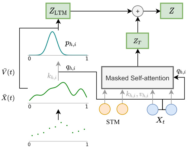
Figure $1\colon\infty$ -former’s attention diagram with sequence of text, $X_{t}$ , of size $L=2$ and STM of size $L_{\mathrm{STM}}=$ 2. Circles represent input embeddings or hidden states (depending on the layer) for head $h$ and query $i$ . Both the self-attention and the attention over the LTM are performed in parallel for each head and query.
图 $1\colon\infty$ -former 在文本序列 $X_{t}$ (长度为 $L=2$) 和 STM (长度为 $L_{\mathrm{STM}}=2$) 情况下的注意力机制示意图。圆圈表示头 $h$ 查询 $i$ 对应的输入嵌入或隐藏状态(具体取决于网络层)。每个头和查询都会并行执行自注意力机制和 LTM 注意力计算。
$B^{\top}=X^{\top}G$ . Then, we can compute the LTM keys, $K_{h}\in\mathbb{R}^{N\times d}$ , and values, $V_{h}\in\mathbb{R}^{N\times d}$ , for each attention head $h$ , as:
$B^{\top}=X^{\top}G$ 。接着,我们可以计算每个注意力头 $h$ 的长时记忆键 $K_{h}\in\mathbb{R}^{N\times d}$ 和值 $V_{h}\in\mathbb{R}^{N\times d}$ ,公式如下:
$$
{\cal K}{h}=B_{h}{\cal W}^{K_{h}},~{\cal V}{h}=B_{h}{\cal W}^{V_{h}},
$$
$$
{\cal K}{h}=B_{h}{\cal W}^{K_{h}},~{\cal V}{h}=B_{h}{\cal W}^{V_{h}},
$$
where $W^{K_{h}}$ , $W^{V_{h}}\in\mathbb{R}^{d\times d}$ are learnable projection matrices.4 For each query $q_{h,i}$ for $i\in{1,\ldots,L}$ , we use a parameterized network, which takes as input the attention scores, to compute $\mu_{h,i}\in]0,1[$ and $\sigma_{h,i}^{2}\in\mathbb{R}_{>0}$ :
其中 $W^{K_{h}}$ 和 $W^{V_{h}}\in\mathbb{R}^{d\times d}$ 是可学习的投影矩阵。对于每个查询 $q_{h,i}$ (其中 $i\in{1,\ldots,L}$),我们使用一个参数化网络,以注意力分数作为输入,计算 $\mu_{h,i}\in]0,1[$ 和 $\sigma_{h,i}^{2}\in\mathbb{R}_{>0}$:
$$
\begin{array}{r l}&{\mu_{h,i}=\mathrm{sigmoid}\left(\mathrm{affnne}\left(\frac{K_{h}q_{h,i}}{\sqrt{d}}\right)\right)}\ &{\sigma_{h,i}^{2}=\mathrm{softplus}\left(\mathrm{affne}\left(\frac{K_{h}q_{h,i}}{\sqrt{d}}\right)\right).}\end{array}
$$
$$
\begin{array}{r l}&{\mu_{h,i}=\mathrm{sigmoid}\left(\mathrm{affnne}\left(\frac{K_{h}q_{h,i}}{\sqrt{d}}\right)\right)}\ &{\sigma_{h,i}^{2}=\mathrm{softplus}\left(\mathrm{affne}\left(\frac{K_{h}q_{h,i}}{\sqrt{d}}\right)\right).}\end{array}
$$
Then, using the continuous softmax transformation (Martins et al., 2020), we obtain the probability density $p_{h,i}$ as $\mathcal{N}(t;\mu_{h,i},\sigma_{h,i}^{2})$ .
然后,使用连续softmax变换 (Martins et al., 2020),我们得到概率密度$p_{h,i}$为$\mathcal{N}(t;\mu_{h,i},\sigma_{h,i}^{2})$。
Finally, having the value function $\bar{V}{h}(t)$ given as ${\bar{V}}{h}(t)=V_{h}^{\top}\psi(t)$ , we compute the head-specific representation vectors as in Eq. 6:
最后,给定价值函数 $\bar{V}{h}(t)$ 为 ${\bar{V}}{h}(t)=V_{h}^{\top}\psi(t)$ ,我们按照公式6计算头部特定表示向量:
$$
z_{h,i}=\mathbb{E}{p_{h,i}}[\bar{V}{h}]=V_{h}^{\top}\mathbb{E}{p_{h,i}}[\psi(t)]
$$
$$
z_{h,i}=\mathbb{E}{p_{h,i}}[\bar{V}{h}]=V_{h}^{\top}\mathbb{E}{p_{h,i}}[\psi(t)]
$$
which form the rows of matrix $Z_{\mathrm{LTM},h}\in\mathbb{R}^{L\times d}$ that goes through an affine transformation, $Z_{\mathrm{LTM}}=[Z_{\mathrm{LTM},1},\dots,Z_{\mathrm{LTM},H}]W^{O}$ .
这些行构成了矩阵 $Z_{\mathrm{LTM},h}\in\mathbb{R}^{L\times d}$ ,经过仿射变换后得到 $Z_{\mathrm{LTM}}=[Z_{\mathrm{LTM},1},\dots,Z_{\mathrm{LTM},H}]W^{O}$ 。
The long-term representation, $Z_{\mathrm{LTM}}$ , is then summed to the transformer context vector, $Z_{\mathrm{T}}$ , to obtain the final context representation $\boldsymbol{Z}\in\mathbb{R}^{L\times e}$ :
长期记忆表示 $Z_{\mathrm{LTM}}$ 随后与 Transformer 上下文向量 $Z_{\mathrm{T}}$ 相加,得到最终的上下文表示 $\boldsymbol{Z}\in\mathbb{R}^{L\times e}$:
$$
Z=Z_{\mathrm{T}}+Z_{\mathrm{LTM}},
$$
$$
Z=Z_{\mathrm{T}}+Z_{\mathrm{LTM}},
$$
which will be the input to the feed-forward layer.
这将成为前馈层的输入。
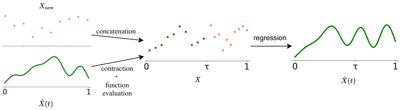
Figure 2: Diagram of the unbounded memory update procedure. This is performed in parallel for each embedding dimension, and repeated throughout the input sequence. We propose two alternatives to select the positions used for the function evaluation: linearly spaced or sticky memories.
图 2: 无界内存更新流程示意图。该过程在每个嵌入维度上并行执行,并在整个输入序列中重复。我们提出了两种选择用于函数评估位置的方案:线性间隔或粘性记忆。
3.1.1 Attention Complexity
3.1.1 注意力复杂度
As the $\infty$ -former makes use of a continuousspace attention framework (Martins et al., 2020) to attend over the LTM signal, its key matrix size ${K_{h}}\in\mathbb{R}^{N\times d}$ depends only on the number of basis functions $N$ , but not on the length of the context being attended to. Thus, the $\infty$ -former’s attention complexity is also independent of the context’s length. It corresponds to $\mathcal{O}(L\times(L+L_{\mathrm{STM}})+L\times N)$ when also using a short-term memory and $\mathcal{O}(L^{2}+L\times N)$ when only using the LTM, both $\ll\mathcal{O}(L\times(L+L_{\mathrm{LTM}}))$ , which would be the complexity of a vanilla transformer attending to the same context. For this reason, the $\infty$ -former can attend to arbitrarily long contexts without increasing the amount of computation needed.
由于 $\infty$-former 采用了连续空间注意力框架 (Martins et al., 2020) 来处理长时记忆 (LTM) 信号,其关键矩阵大小 ${K_{h}}\in\mathbb{R}^{N\times d}$ 仅取决于基函数数量 $N$,而与待处理上下文的长度无关。因此,$\infty$-former 的注意力计算复杂度也与上下文长度无关。当同时使用短时记忆时,复杂度为 $\mathcal{O}(L\times(L+L_{\mathrm{STM}})+L\times N)$;仅使用长时记忆时,复杂度为 $\mathcal{O}(L^{2}+L\times N)$。这两种情况都远小于传统 Transformer 处理相同上下文时的复杂度 $\mathcal{O}(L\times(L+L_{\mathrm{LTM}}))$。正因如此,$\infty$-former 能够处理任意长度的上下文而无需增加计算量。
3.2 Unbounded Memory
3.2 无限内存
When representing the memory as a discrete sequence, to extend it, we need to store the new hidden states in memory. In a vanilla transformer, this is not feasible for long contexts due to the high memory requirements. However, the $\infty$ -former can attend to unbounded context without increasing memory requirements by using continuous attention, as next described and shown in Fig. 2.
当将记忆表示为离散序列时,为了扩展它,我们需要将新的隐藏状态存储在内存中。在普通的Transformer中,由于内存需求较高,这对于长上下文是不可行的。然而,$\infty$-former可以通过使用连续注意力来关注无界上下文,而不会增加内存需求,如下所述并在图2中展示。
To be able to build an unbounded representation, we first sample $M$ locations in [0, 1] and evaluate $\bar{X}(t)$ at those locations. These locations can simply be linearly spaced, or sampled according to the region importance, as described in $\S3.3$ .
为了构建无界表示,我们首先在[0, 1]区间内采样$M$个位置,并在这些位置上评估$\bar{X}(t)$。这些位置可以简单地线性间隔分布,或根据$\S3.3$中描述的区域重要性进行采样。
Then, we concatenate the corresponding vectors with the new vectors coming from the short-term memory. For that, we first need to contract this function by a factor of $\tau\in]0,1[$ to make room for the new vectors. We do this by defining:
然后,我们将对应的向量与来自短期记忆的新向量进行拼接。为此,我们首先需要将该函数按因子 $\tau\in]0,1[$ 收缩,以便为新向量腾出空间。具体定义如下:
$$
X^{\mathrm{contracted}}(t)=X(t/\tau)=B^{\top}\psi(t/\tau).
$$
$$
X^{\mathrm{contracted}}(t)=X(t/\tau)=B^{\top}\psi(t/\tau).
$$
Then, we can evaluate ${\bar{X}}(t)$ at the $M$ locations $0\leq t_{1},t_{2},\dots,t_{M}\leq\tau$ as:
然后,我们可以在 $M$ 个位置 $0\leq t_{1},t_{2},\dots,t_{M}\leq\tau$ 处评估 ${\bar{X}}(t)$:
$$
x_{m}=B^{\top}\psi(t_{m}/\tau),\quad{\mathrm{for~}}m\in[M],
$$
$$
x_{m}=B^{\top}\psi(t_{m}/\tau),\quad{\mathrm{for~}}m\in[M],
$$
and define a matrix $X_{\mathrm{past}}=[x_{1},x_{2},\ldots,x_{M}]^{\top}\in$ $\mathbb{R}^{M\times e}$ with these vectors as rows. After that, we concatenate this matrix with the new vectors $X_{\mathrm{new}}$ , obtaining:
并定义一个矩阵 $X_{\mathrm{past}}=[x_{1},x_{2},\ldots,x_{M}]^{\top}\in$ $\mathbb{R}^{M\times e}$,将这些向量作为行。之后,我们将该矩阵与新向量 $X_{\mathrm{new}}$ 拼接,得到:
$$
\begin{array}{r}{X=\Big[X_{\mathrm{past}}^{\top},X_{\mathrm{new}}^{\top}\Big]^{\top}\in\mathbb{R}^{(M+L)\times e}.}\end{array}
$$
$$
\begin{array}{r}{X=\Big[X_{\mathrm{past}}^{\top},X_{\mathrm{new}}^{\top}\Big]^{\top}\in\mathbb{R}^{(M+L)\times e}.}\end{array}
$$
Finally, we simply need to perform multivariate ridge regression to compute the new coefficient matrix $\boldsymbol{B}\in\mathbb{R}^{N\times e}$ , via $B^{\top}=X^{\top}G$ , as in Eq. 5. To do this, we need to associate the vectors in $X_{\mathrm{past}}$ with positions in $[0,\tau]$ and in $X_{\mathrm{new}}$ with positions in $\left]\tau,1\right]$ so that we obtain the matrix $G\in\mathbb{R}^{(M+L)\times N}$ . We consider the vectors positions to be linearly spaced.
最后,我们只需执行多元岭回归来计算新的系数矩阵 $\boldsymbol{B}\in\mathbb{R}^{N\times e}$,通过 $B^{\top}=X^{\top}G$,如公式5所示。为此,我们需要将 $X_{\mathrm{past}}$ 中的向量与 $[0,\tau]$ 区间内的位置关联,并将 $X_{\mathrm{new}}$ 中的向量与 $\left]\tau,1\right]$ 区间内的位置关联,从而得到矩阵 $G\in\mathbb{R}^{(M+L)\times N}$。我们假设这些向量的位置是线性分布的。
3.3 Sticky Memories
3.3 粘性记忆
When extending the LTM, we evaluate its current signal at $M$ locations in $[0,1]$ , as shown in Eq. 14. These locations can be linearly spaced. However, some regions of the signal can be more relevant than others, and should consequently be given a larger “memory space” in the next step LTM’s signal. To take this into account, we propose sampling the $M$ locations according to the signal’s relevance at each region (see Fig. 6 in App. B). To do so, we construct a histogram based on the attention given to each interval of the signal on the previous step. For that, we first divide the signal into
在扩展长时记忆(LTM)时,我们会在$[0,1]$区间内选取$M$个位置评估当前信号,如公式14所示。这些位置可以线性均匀分布。然而,信号的某些区域可能比其他区域更重要,因此应在下一步LTM信号中分配更大的"记忆空间"。为此,我们提出根据信号各区域的相关性来采样这$M$个位置(参见附录B中的图6)。具体实现时,我们基于上一步信号各区间获得的注意力构建直方图。首先将信号划分为...
$D$ linearly spaced bins ${d_{1},\ldots,d_{D}}$ . Then, we compute the probability given to each bin, $p(d_{j})$ for $j\in{1,\ldots,D}$ , as:
$D$ 个线性间隔的区间 ${d_{1},\ldots,d_{D}}$。然后,我们计算每个区间的概率 $p(d_{j})$,其中 $j\in{1,\ldots,D}$,公式如下:
$$
p(d_{j})\propto\sum_{h=1}^{H}\sum_{i=1}^{L}\int_{d_{j}}\mathcal{N}(t;\mu_{h,i},\sigma_{h,i}^{2})~d t,
$$
$$
p(d_{j})\propto\sum_{h=1}^{H}\sum_{i=1}^{L}\int_{d_{j}}\mathcal{N}(t;\mu_{h,i},\sigma_{h,i}^{2})~d t,
$$
where $H$ is the number of attention heads and $L$ is the sequence length. Note that Eq. 16’s integral can be evaluated efficiently using the erf function:
其中 $H$ 是注意力头(attention head)的数量,$L$ 是序列长度。需要注意的是,公式(16)的积分可以通过erf函数高效计算:
$$
\int_{a}^{b}{\mathcal{N}}(t;\mu,\sigma^{2})={\frac{1}{2}}{\bigg(}\mathrm{erf}{\bigg(}{\frac{b}{\sqrt{2}}}{\bigg)}-\mathrm{erf}{\bigg(}{\frac{a}{\sqrt{2}}}{\bigg)}{\bigg)}.
$$
$$
\int_{a}^{b}{\mathcal{N}}(t;\mu,\sigma^{2})={\frac{1}{2}}{\bigg(}\mathrm{erf}{\bigg(}{\frac{b}{\sqrt{2}}}{\bigg)}-\mathrm{erf}{\bigg(}{\frac{a}{\sqrt{2}}}{\bigg)}{\bigg)}.
$$
Then, we sample the $M$ locations at which the LTM’s signal is evaluated at, according to $p$ . By doing so, we evaluate the LTM’s signal at the regions which were considered more relevant by the previous step’s attention, and will, consequently attribute a larger space of the new LTM’s signal to the memories stored in those regions.
然后,我们根据 $p$ 对评估长时记忆 (LTM) 信号的 $M$ 个位置进行采样。通过这种方式,我们在上一步注意力认为更相关的区域评估长时记忆信号,从而将新长时记忆信号的更大空间归因于存储在这些区域的记忆。
3.4 Implementation and Learning Details
3.4 实现与学习细节
Discrete sequences can be highly irregular and, consequently, difficult to convert into a continuous signal through regression. Because of this, before applying multivariate ridge regression to convert the discrete sequence $X$ into a continuous signal, we use a simple convolutional layer (with stride $=$ 1 and width $=3$ ) as a gate, to smooth the sequence:
离散序列可能高度不规则,因此难以通过回归转换为连续信号。因此,在应用多元岭回归将离散序列 $X$ 转换为连续信号之前,我们使用一个简单的卷积层(步长 $=1$,宽度 $=3$)作为门控机制来平滑序列:
$$
\tilde{X}=\mathsf{s i g m o i d}\left(\mathrm{CNN}(X)\right)\odot X.
$$
$$
\tilde{X}=\mathsf{s i g m o i d}\left(\mathrm{CNN}(X)\right)\odot X.
$$
To train the model we use the cross entropy loss. Having a sequence of text $X$ of length $L$ as input, a language model outputs a probability distribution of the next word $p(x_{t+1}\mid x_{t},\ldots,x_{t-L})$ . Given a corpus of $T$ tokens, we train the model to minimize its negative log likelihood:
为了训练模型,我们使用交叉熵损失。给定一个长度为 $L$ 的文本序列 $X$ 作为输入,语言模型会输出下一个词的概率分布 $p(x_{t+1}\mid x_{t},\ldots,x_{t-L})$。给定一个包含 $T$ 个 token 的语料库,我们训练模型以最小化其负对数似然:
get:
获取:
$$
\mathcal{L}{\mathrm{KL}}=\sum_{t=0}^{T-1}\sum_{h=1}^{H}D_{\mathrm{KL}}\left(\mathcal{N}(\mu_{h},\sigma_{h})||\mathcal{N}(\mu_{h},\sigma_{0})\right)
$$
$$
\mathcal{L}{\mathrm{KL}}=\sum_{t=0}^{T-1}\sum_{h=1}^{H}D_{\mathrm{KL}}\left(\mathcal{N}(\mu_{h},\sigma_{h})||\mathcal{N}(\mu_{h},\sigma_{0})\right)
$$
$$
=\sum_{t=0}^{T-1}\sum_{h=1}^{H}\frac{1}{2}\Bigg(\frac{\sigma_{h}^{2}}{\sigma_{0}^{2}}-\log\Bigg(\frac{\sigma_{h}}{\sigma_{0}}\Bigg)-1\Bigg).
$$
$$
=\sum_{t=0}^{T-1}\sum_{h=1}^{H}\frac{1}{2}\Bigg(\frac{\sigma_{h}^{2}}{\sigma_{0}^{2}}-\log\Bigg(\frac{\sigma_{h}}{\sigma_{0}}\Bigg)-1\Bigg).
$$
Thus, the final loss that is minimized corresponds to:
因此,最终被最小化的损失对应于:
$$
\begin{array}{r}{\mathcal{L}=\mathcal{L}{\mathrm{NLL}}+\lambda_{\mathrm{KL}}\mathcal{L}_{\mathrm{KL}},}\end{array}
$$
$$
\begin{array}{r}{\mathcal{L}=\mathcal{L}{\mathrm{NLL}}+\lambda_{\mathrm{KL}}\mathcal{L}_{\mathrm{KL}},}\end{array}
$$
where $\lambda_{\mathrm{KL}}$ is a hyper parameter that controls the amount of KL regular iz ation.
其中 $\lambda_{\mathrm{KL}}$ 是控制KL正则化量的超参数。
4 Experiments
4 实验
To understand if the $\infty$ -former is able to model long contexts, we first performed experiments on a synthetic task, which consists of sorting tokens by their frequencies in a long sequence (§4.1). Then, we performed experiments on language modeling (§4.2) and document grounded dialogue generation (§4.3) by fine-tuning a pre-trained language model.5
为了验证$\infty$-former能否建模长上下文,我们首先在一项合成任务上进行了实验,该任务要求根据token在长序列中的出现频率对其进行排序(见4.1节)。接着,我们通过对预训练语言模型进行微调,在语言建模(见4.2节)和基于文档的对话生成(见4.3节)任务上展开了实验。
4.1 Sorting
4.1 排序
In this task, the input consists of a sequence of tokens sampled according to a token probability distribution (which is not known to the system). The goal is to generate the tokens in the decreasing order of their frequencies in the sequence. One example can be:
在此任务中,输入由根据token概率分布(系统未知该分布)采样得到的一系列token组成。目标是根据这些token在序列中出现频率的降序来生成它们。一个示例如下:
$$
{\mathcal{L}}{\mathrm{NLL}}=-\sum_{t=0}^{T-1}\log p(x_{t+1}\mid x_{t},\ldots,x_{t-L}).
$$
$$
{\mathcal{L}}{\mathrm{NLL}}=-\sum_{t=0}^{T-1}\log p(x_{t+1}\mid x_{t},\ldots,x_{t-L}).
$$
Additionally, in order to avoid having uniform distributions over the LTM, we regularize the continuous attention given to the LTM, by minimizing the Kullback-Leibler (KL) divergence, $D_{\mathrm{KL}}$ , between the attention probability density, $\mathcal{N}(\mu_{h},\sigma_{h})$ , and a Gaussian prior, $\mathcal{N}(\mu_{0},\sigma_{0})$ . As different heads can attend to different regions, we set $\mu_{0}=$ $\mu_{h}$ , regularizing only the attention variance, and
此外,为避免长时记忆 (LTM) 上出现均匀分布,我们通过最小化注意力概率密度 $\mathcal{N}(\mu_{h},\sigma_{h})$ 与高斯先验 $\mathcal{N}(\mu_{0},\sigma_{0})$ 之间的 Kullback-Leibler (KL) 散度 $D_{\mathrm{KL}}$ 来正则化对 LTM 的持续注意力。由于不同注意力头可关注不同区域,我们设 $\mu_{0}=$ $\mu_{h}$ ,仅正则化注意力方差,且
To understand if the long-term memory is being effectively used and the transformer is not only performing sorting by modeling the most recent tokens, we design the token probability distribution to change over time: namely, we set it as a mixture of two distributions, $p=\alpha p_{0}+(1-\alpha)p_{1}$ , where the mixture coefficient $\alpha\in[0,1]$ is progressively increased from 0 to 1 as the sequence is generated. The vocabulary has 20 tokens and we experiment with sequences of length 4,000, 8,000, and 16,000.
为了验证长期记忆是否被有效利用,以及Transformer是否不仅通过建模最近token来进行排序,我们设计了随时间变化的token概率分布:具体而言,将其设置为两个分布的混合形式 $p=\alpha p_{0}+(1-\alpha)p_{1}$ ,其中混合系数 $\alpha\in[0,1]$ 会随着序列生成过程从0逐步增加到1。词汇表包含20个token,我们分别对长度为4,000、8,000和16,000的序列进行了实验。
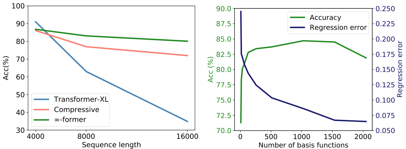
Figure 3: Left: Sorting task accuracy for sequences of length 4,000, 8,000, and 16,000. Right: Sorting task accuracy vs regression mean error, when varying the number of basis functions, for sequences of length 8,000.
图 3: 左: 长度为 4,000、8,000 和 16,000 的序列排序任务准确率。右: 在长度为 8,000 的序列上,改变基函数数量时的排序任务准确率与回归平均误差对比。
Baselines. We consider the transformer-XL6 (Dai et al., 2019) and the compressive transformer 7 (Rae et al., 2019) as baselines. The transformer-XL consists of a vanilla transformer (Vaswani et al., 2017) extended with a short-term memory which is composed of the hidden states of the previous steps. The compressive transformer is an extension of the transformer-XL: besides the short-term memory, it has a compressive long-term memory which is composed of the old vectors of the short-term memory, compressed using a CNN. Both the transformer-XL and the compressive transformer require relative positional encodings. In contrast, there is no need for positional encodings in the memory in our approach since the memory vectors represent basis coefficients in a predefined continuous space.
基线方法。我们选择 transformer-XL6 (Dai et al., 2019) 和 compressive transformer7 (Rae et al., 2019) 作为基线。transformer-XL 由基础 Transformer (Vaswani et al., 2017) 扩展而来,增加了由前几步隐藏状态组成的短期记忆模块。compressive transformer 是 transformer-XL 的扩展:除了短期记忆外,它还包含一个压缩长期记忆模块,该模块由经过 CNN 压缩的短期记忆旧向量组成。transformer-XL 和 compressive transformer 都需要相对位置编码。相比之下,我们的方法中记忆向量不需要位置编码,因为这些向量表示预定义连续空间中的基系数。
For all models we used a transformer with 3 layers and 6 attention heads, input size $L=1,024$ and memory size 2,048. For the compressive transformer, both memories have size 1,024. For the $\infty$ -former, we also consider a STM of size 1,024 and a LTM with $N=1,024$ basis functions, having the models the same computational cost. Further details are described in App. C.1.
我们使用的所有模型均为3层6注意力头的Transformer架构,输入尺寸$L=1,024$,记忆体容量2,048。其中压缩Transformer的两个记忆体容量均为1,024。对于$\infty$-former,我们还配置了容量1,024的短期记忆(STM)和含$N=1,024$个基函数的长期记忆(LTM),确保各模型计算成本一致。更多细节详见附录C.1。
Results. As can be seen in the left plot of Fig. 3, the transformer-XL achieves a slightly higher accuracy than the compressive transformer and $\infty$ -former for a short sequence length (4,000). This is because the transformer-XL is able to keep almost the entire sequence in memory. However, its accuracy degrades rapidly when the sequence length is increased. Both the compressive transformer and $\infty$ -former also lead to smaller accuracies when increasing the sequence length, as expected. However, this decrease is not so significant for the $\infty$ -former, which indicates that it is better at modeling long sequences.
结果。如图 3 左图所示,在短序列长度 (4,000) 下,transformer-XL 的准确率略高于 compressive transformer 和 $\infty$-former。这是因为 transformer-XL 能够将几乎整个序列保留在内存中。然而,当序列长度增加时,其准确率会迅速下降。正如预期的那样,compressive transformer 和 $\infty$-former 在增加序列长度时也会导致准确率下降。但对于 $\infty$-former 而言,这种下降并不显著,这表明它在建模长序列方面表现更优。
Regression error analysis. To better understand the trade-off between the $\infty$ -former’s memory precision and its computational efficiency, we analyze how its regression error and sorting accuracy vary when varying the number of basis functions used, on the sorting task with input sequences of length 8,000. As can be seen in the right plot of Fig. 3, the sorting accuracy is negatively correlated with the regression error, which is positively correlated with the number of basis functions. It can also be observed, that when increasing substantially the number of basis functions the regression error reaches a plateau and the accuracy starts to drop. We posit that the latter is caused by the model having a harder task at selecting the locations it should attend to. This shows that, as expected, when increasing $\infty$ -former’s efficiency or increasing the size of context being modeled, the memory loses precision.
回归误差分析。为了更好地理解 $\infty$-former 的记忆精度与计算效率之间的权衡,我们分析了在长度为 8,000 的输入序列排序任务中,其回归误差和排序准确率如何随使用的基函数数量变化而变化。如图 3 右图所示,排序准确率与回归误差呈负相关,而回归误差与基函数数量呈正相关。还可以观察到,当大幅增加基函数数量时,回归误差达到平台期,而准确率开始下降。我们认为后者是由于模型在选择应关注的位置时面临更困难的任务。这表明,正如预期的那样,当提高 $\infty$-former 的效率或增加建模上下文的大小时,记忆会失去精度。
4.2 Language Modeling
4.2 语言建模
To understand if long-term memories can be used to extend a pre-trained language model, we fine-tune GPT-2 small (Radford et al., 2019) on Wikitext- 103 (Merity et al., 2017) and a subset of PG-19 (Rae et al., 2019) containing the first 2,000 books ( $\approx200$ million tokens) of the training set. To do so, we extend GPT-2 with a continuous long-term memory ( $\mathrm{\infty}$ -former) and a compressed memory (compressive transformer) with a positional bias,
为了验证长期记忆能否用于扩展预训练语言模型,我们在Wikitext-103 (Merity et al., 2017) 和PG-19训练集前2000本书籍(约2亿token)子集 (Rae et al., 2019) 上对GPT-2 small (Radford et al., 2019) 进行微调。具体实现中,我们通过以下两种方式扩展GPT-2:带位置偏置的连续长期记忆 ( $\mathrm{\infty}$ -former) 和压缩记忆 (compressive transformer) 。
Table 1: Perplexity on Wikitext-103 and PG19.
表 1: Wikitext-103 和 PG19 上的困惑度。
| Wikitext-103 | PG19 | |
|---|---|---|
| GPT-2 | 16.85 | 33.44 |
| Compressive | 16.87 | 33.09 |
| o-former | 16.64 | 32.61 |
| -former (SM) | 16.61 | 32.48 |
based on Press et al. (2021).8
基于 Press 等人 (2021) 的研究。8
For these experiments, we consider transformers with input size $L=512$ , for the compressive transformer we use a compressed memory of size 512, and for the $\infty$ -former we consider a LTM with $N=512$ Gaussian RBFs and a memory threshold of 2,048 tokens, having the same computational budget for the two models. Further details and hyper parameters are described in App. C.2.
在这些实验中,我们考虑输入尺寸为 $L=512$ 的 Transformer。对于压缩 Transformer,我们使用大小为 512 的压缩记忆;对于 $\infty$ -former,我们考虑具有 $N=512$ 个高斯径向基函数 (Gaussian RBFs) 的长时记忆 (LTM) 和 2,048 个 Token 的记忆阈值,确保两种模型的计算预算相同。更多细节和超参数详见附录 C.2。
Results. The results reported in Table 1 show that the $\infty$ -former leads to perplexity improvements on both Wikitext-103 and PG19, while the compressive transformer only has a slight improvement on the latter. The improvements obtained by the $\infty$ -former are larger on the PG19 dataset, which can be justified by the nature of the datasets: books have more long range dependencies than Wikipedia articles (Rae et al., 2019).
结果。表1中报告的结果表明,$\infty$-former在Wikitext-103和PG19上都带来了困惑度(perplexity)提升,而压缩Transformer(compressive transformer)仅在后一个数据集上有轻微改进。$\infty$-former在PG19数据集上获得的改进更大,这可以通过数据集的特性来解释:书籍比维基百科文章具有更长程的依赖关系(Rae等人,2019)[20]。
4.3 Document Grounded Dialogue
4.3 文档基础对话
In document grounded dialogue generation, besides the dialogue history, models have access to a document concerning the conversation’s topic. In the CMU Document Grounded Conversation dataset (CMU-DoG) (Zhou et al., 2018), the dialogues are about movies and a summary of the movie is given as the auxiliary document; the auxiliary document is divided into parts that should be considered for the different utterances of the dialogue. In this paper, to evaluate the usefulness of the long-term memories, we make this task slightly more challenging by only giving the models access to the document before the start of the dialogue.
在基于文档的对话生成任务中,除了对话历史外,模型还能获取与话题相关的文档。CMU基于文档的对话数据集(CMU-DoG) (Zhou et al., 2018)中的对话以电影为主题,并提供了电影摘要作为辅助文档;该辅助文档被划分为多个部分,分别对应对话中不同话语的参考内容。本文为评估长期记忆的有效性,通过仅在对话开始前向模型提供文档的方式,略微提升了该任务的挑战性。
We fine-tune GPT-2 small (Radford et al., 2019) using an approach based on Wolf et al. (2019). To allow the model to keep the whole document on memory, we extend GPT-2 with a continuous LTM ( $\infty$ -former) with $N=512$ basis functions. As baselines, we use GPT-2, with and without access (GPT-2 w/o doc) to the auxiliary document, with input size $L=512$ , and GPT-2 with a compressed memory with attention positional biases (compressive), of size 512. Further details and hyper-parameters are stated in App. C.3.
我们采用基于Wolf等人(2019)的方法对GPT-2 small (Radford等人,2019)进行微调。为了让模型能够将整个文档保留在内存中,我们通过一个包含$N=512$个基函数的连续LTM( $\infty$ -former)对GPT-2进行了扩展。作为基线,我们使用了GPT-2(在有/无辅助文档访问权限(GPT-2 w/o doc)的情况下),输入尺寸为$L=512$,以及带有注意力位置偏置的压缩内存(compressive)、尺寸为512的GPT-2。更多细节和超参数见附录C.3。
Table 2: Results on CMU-DoG dataset.
| PPL | F1 | Rouge-1 | Rouge-L | Meteor | |
| GPT-2w/odoc | 19.43 | 7.82 | 12.18 | 10.17 | 6.10 |
| GPT-2 | 18.53 | 8.64 | 14.61 | 12.03 | 7.15 |
| Compressive | 18.02 | 8.78 | 14.74 | 12.14 | 7.29 |
| -former | 18.02 | 8.92 | 15.28 | 12.51 | 7.52 |
| -former (SM) | 18.04 | 9.01 | 15.37 | 12.56 | 7.55 |
表 2: CMU-DoG数据集上的结果。
| PPL | F1 | Rouge-1 | Rouge-L | Meteor | |
|---|---|---|---|---|---|
| GPT-2w/odoc | 19.43 | 7.82 | 12.18 | 10.17 | 6.10 |
| GPT-2 | 18.53 | 8.64 | 14.61 | 12.03 | 7.15 |
| Compressive | 18.02 | 8.78 | 14.74 | 12.14 | 7.29 |
| -former | 18.02 | 8.92 | 15.28 | 12.51 | 7.52 |
| -former (SM) | 18.04 | 9.01 | 15.37 | 12.56 | 7.55 |
To evaluate the models we use the metrics: perplexity, F1 score, Rouge-1 and Rouge-L (Lin, 2004), and Meteor (Banerjee and Lavie, 2005).
为评估模型性能,我们采用以下指标:困惑度 (perplexity)、F1分数、Rouge-1与Rouge-L (Lin, 2004) 以及Meteor (Banerjee and Lavie, 2005)。
Results. As shown in Table 2, by keeping the whole auxiliary document in memory, the $\infty$ -former and the compressive transformer are able to generate better utterances, according to all metrics. While the compressive and $\infty$ -former achieve essentially the same perplexity in this task, the $\infty$ -former achieves consistently better scores on all other metrics. Also, using sticky memories leads to slightly better results on those metrics, which suggests that attributing a larger space in the LTM to the most relevant tokens can be beneficial.
结果。如表 2 所示,通过将整个辅助文档保留在内存中,$\infty$-former 和 compressive transformer 能够根据所有指标生成更好的话语。虽然 compressive 和 $\infty$-former 在此任务中基本达到了相同的困惑度 (perplexity),但 $\infty$-former 在所有其他指标上始终获得更好的分数。此外,使用 sticky memories 在这些指标上带来了略微更好的结果,这表明在 LTM 中为最相关的 token 分配更大的空间可能是有益的。
Analysis. In Fig. 4, we show examples of ut- terances generated by $\infty$ -former along with the excerpts from the LTM that receive higher attention throughout the utterances’ generation. In these examples, we can clearly see that these excerpts are highly pertinent to the answers being generated. Also, in Fig. 5, we can see that the phrases which are attributed larger spaces in the LTM, when using sticky memories, are relevant to the conversations.
分析。在图4中,我们展示了由$\infty$-former生成的语句示例,以及在整个语句生成过程中获得较高关注度的长期记忆(LTM)片段。通过这些示例可以清晰看出,这些片段与正在生成的答案高度相关。此外,在图5中可见,当使用粘性记忆(sticky memories)时,那些在LTM中被分配较大空间的短语都与对话内容相关。
5 Related Work
5 相关工作
Continuous attention. Martins et al. (2020) introduced 1D and 2D continuous attention, using Gaussians and truncated parabolas as densities. They applied it to RNN-based document classification, machine translation, and visual question answering. Several other works have also proposed the use of (disc ret i zed) Gaussian attention for natural language processing tasks: Guo et al. (2019) proposed a Gaussian prior to the self-attention mechanism to bias the model to give higher attention to nearby words, and applied it to natural lan- guage inference; You et al. (2020) proposed the use
连续注意力。Martins等人 (2020) 提出了使用高斯分布和截断抛物线作为密度函数的1D和2D连续注意力机制,并将其应用于基于RNN的文档分类、机器翻译和视觉问答任务。其他多项研究也提出了将(离散化)高斯注意力用于自然语言处理任务:Guo等人 (2019) 在自注意力机制中引入高斯先验,使模型更关注邻近词语,并将其应用于自然语言推理任务;You等人 (2020) 提出了...
Cast: Macaulay Culkin as Kevin. Joe Pesci as Harry. Daniel Stern as Marv. John Heard as Peter. Roberts Blossom as Marley.
演员表:
Macaulay Culkin 饰 Kevin
Joe Pesci 饰 Harry
Daniel Stern 饰 Marv
John Heard 饰 Peter
Roberts Blossom 饰 Marley
The film stars Macaulay Culkin as Kevin McCall is ter, a boy who is mistakenly left behind when his family flies to Paris for their Christmas vacation. Kevin initially relishes being home alone, but soon has to contend with two would-be burglars played by Joe Pesci and Daniel Stern. The film also features Catherine O'Hara and John Heard as Kevin's parents.
影片由麦考利·卡尔金饰演凯文·麦卡利斯特,一个在家人飞往巴黎过圣诞假期时被意外落下的男孩。凯文起初享受独自在家的自由,但很快不得不面对由乔·佩西和丹尼尔·斯特恩饰演的两名企图行窃的盗贼。凯文的父母则由凯瑟琳·欧哈拉和约翰·赫德出演。
Movie Name: Home Alone. Rating: Rotten Tomatoes: $62%$ and average: 5.5/10, Metacritic Score: 63/100, Cinema Score: A. Year: 1990. The McCall is ter family is preparing to spend Christmas in Paris, gathering at Peter and Kate's home outside of Chicago on the night before their departure. Peter and Kate's youngest son, eightyear-old Kevin, is being ridiculed by his siblings and cousins. A fight with his older brother, Buzz, results in Kevin getting sent to the third floor of the house for punishment, where he wishes that his
电影名称:小鬼当家。评分:烂番茄:$62%$,平均分:5.5/10;Metacritic评分:63/100;影院评分:A。年份:1990。McCallister一家正准备前往巴黎过圣诞节,出发前一晚聚集在Peter和Kate位于芝加哥郊外的家中。Peter和Kate的小儿子、八岁的Kevin正被兄弟姐妹和表亲们嘲笑。与哥哥Buzz的一场争执导致Kevin被罚到房子的三楼,在那里他许愿让他的...
Previous utterance: Or maybe rent, anything is reason to celebrate..I would like to talk about a movie called "Home Alone"
上句:或者也许是房租,任何事都值得庆祝...我想聊聊一部叫《小鬼当家》的电影
Answer: Macaulay Culkin is the main actor and it is a comedy.
答案:Macaulay Culkin是主演,这是一部喜剧。
Previous utterance: That sounds like a great movie. Any more details?
上一条对话:听起来是部很棒的电影。能再详细说说吗?
Answer: The screenplay came out in 1990 and has been on the air for quite a while.
答:该剧本于1990年问世,并已播出相当长一段时间。
Figure 4: Examples of answers generated by $\infty$ -former on a dialogue about the movie “Home Alone”. The excerpts from the LTM that are more attended to throughout the utterances generation are highlighted on each color, correspondingly.
图 4: $\infty$ -former在关于电影《小鬼当家》的对话中生成的回答示例。在生成话语过程中,从长时记忆(LTM)中提取的、受到更多关注的部分分别以对应颜色高亮显示。
Toy Story: Tom Hanks as Woody | animated buddy comedy | Toy Story was the first feature length computer animated film | produced by Pixar | toys pretend to be lifeless whenever humans are present | focuses on the relationship between Woody and Gold | fashioned pull string cowboy doll
玩具总动员:Tom Hanks配音Woody | 动画伙伴喜剧 | 首部全电脑动画长片 | 皮克斯制作 | 人类在场时玩具装成无生命体 | 聚焦Woody与Gold的关系 | 拉线牛仔玩偶造型
La La Land: Ryan Gosling | Emma Stone as Mia | Hollywood | the city of Los Angeles | Meta critics: 93/100 | 2016 | During a gig at a restaurant Sebastian slips into a passionate jazz | despite warning from the owner | Mia overhears the music as she passes by | for his disobedience
爱乐之城: Ryan Gosling | Emma Stone 饰演 Mia | 好莱坞 | 洛杉矶 | 烂番茄评分: 93/100 | 2016年 | Sebastian在餐厅演出时不顾老板警告即兴演奏激情爵士乐 | 路过的Mia被琴声吸引
Figure 5: Phrases that hold larger spaces of the LTM, when using sticky memories, for two dialogue examples (in App. E).
图 5: 使用粘性记忆时,两个对话示例中占据长期记忆 (LTM) 更大空间的短语 (见附录 E)。
of hard-coded Gaussian attention as input-agnostic self-attention layer for machine translation; Dubois et al. (2020) proposed using Gaussian attention as a location attention mechanism to improve the model generalization to longer sequences. However, these approaches still consider discrete sequences and compute the attention by evaluating the Gaussian density at the token positions. Farinhas et al. (2021) extend continuous attention to multimodal densities, i.e., mixtures of Gaussians, and applied it to VQA. In this paper, we opt for the simpler case, an unimodal Gaussian, and leave sparse and multimodal continuous attention for future work.
在机器翻译中使用硬编码高斯注意力作为输入无关的自注意力层;Dubois等人(2020)提出将高斯注意力作为位置注意力机制,以提升模型对长序列的泛化能力。然而这些方法仍考虑离散序列,并通过在token位置评估高斯密度来计算注意力。Farinhas等人(2021)将连续注意力扩展到多模态密度(即高斯混合分布),并应用于视觉问答(VQA)。本文选择更简单的单峰高斯分布,将稀疏和多模态连续注意力留作未来研究方向。
Efficient transformers. Several methods have been proposed that reduce the transformer’s attention complexity, and can, consequently, model longer contexts. Some of these do so by performing sparse attention, either by selecting pre-defined attention patterns (Child et al., 2019; Beltagy et al., 2020; Zaheer et al., 2020), or by learning these patterns from data (Kitaev et al., 2020; Vyas et al., 2020; Tay et al., 2020a; Roy et al., 2021; Wang et al., 2021). Other works focus on directly reducing the attention complexity by applying the (reversed) kernel trick (Katha ro poul os et al., 2020; Cho roman ski et al., 2021; Peng et al., 2021; Jae- gle et al., 2021). Closer to our approach are the transformer-XL and compressive transformer models (Dai et al., 2019; Rae et al., 2019), which extend the vanilla transformer with a bounded memory.
高效Transformer。目前已提出多种方法来降低Transformer的注意力复杂度,从而能够建模更长的上下文。其中一些方法通过执行稀疏注意力来实现,要么选择预定义的注意力模式 (Child等人, 2019; Beltagy等人, 2020; Zaheer等人, 2020),要么从数据中学习这些模式 (Kitaev等人, 2020; Vyas等人, 2020; Tay等人, 2020a; Roy等人, 2021; Wang等人, 2021)。其他工作则侧重于通过应用(反向)核技巧直接降低注意力复杂度 (Katharopoulos等人, 2020; Choromanski等人, 2021; Peng等人, 2021; Jaegle等人, 2021)。与我们的方法更接近的是transformer-XL和压缩Transformer模型 (Dai等人, 2019; Rae等人, 2019),它们通过有限内存扩展了原始Transformer。
Memory-augmented language models. RNNs, LSTMs, and GRUs (Hochreiter et al., 1997; Cho et al., 2014) have the ability of keeping a memory state of the past. However, these require backpropagation through time which is impractical for long sequences. Because of this, Graves et al. (2014), Weston et al. (2014), Joulin and Mikolov (2015) and Gre fens te tte et al. (2015) proposed extending RNNs with an external memory, while Chandar et al. (2016) and Rae et al. (2016) proposed efficient procedures to read and write from these memories, using hierarchies and sparsity. Grave et al. (2016) and Merity et al. (2017) proposed the use of cache-based memories which store pairs of hidden states and output tokens from previous steps. The distribution over the words in the memory is then combined with the distribution given by the language model. More recently, Khandelwal et al. (2019) and Yogatama et al. (2021) proposed using nearest neighbors to retrieve words from a keybased memory constructed based on the training data. Similarly, Fan et al. (2021) proposed retrieving sentences from a memory based on the training data and auxiliary information. Khandelwal et al. (2019) proposed interpolating the retrieved words probability distributions with the probability over the vocabulary words when generating a new word, while Yogatama et al. (2021) and Fan et al. (2021) proposed combining the information at the architecture level. These models have the disadvantage of needing to perform a retrieval step when generating each token / utterance, which can be computationally expensive. These approaches are orthogonal to the $\infty$ -former’s LTM and in future work the two can be combined.
记忆增强语言模型。RNN、LSTM和GRU (Hochreiter et al., 1997; Cho et al., 2014) 具备保留历史记忆状态的能力,但需要通过时间反向传播,这对长序列而言并不实用。为此,Graves et al. (2014)、Weston et al. (2014)、Joulin and Mikolov (2015) 以及 Gre fens te tte et al. (2015) 提出了通过外部记忆扩展RNN的方案,而Chandar et al. (2016) 和 Rae et al. (2016) 则利用层级结构与稀疏性设计了高效的记忆读写机制。Grave et al. (2016) 与 Merity et al. (2017) 提出基于缓存的记忆系统,存储历史隐藏状态与输出token的配对信息,并将记忆中的词汇分布与语言模型给出的分布相结合。近期,Khandelwal et al. (2019) 和 Yogatama et al. (2021) 提出通过最近邻方法从基于训练数据构建的键值记忆中检索词汇,Fan et al. (2021) 则提出根据训练数据与辅助信息检索句子。Khandelwal et al. (2019) 在生成新词时采用检索词汇概率分布与词表概率分布的插值策略,而 Yogatama et al. (2021) 和 Fan et al. (2021) 主张在架构层面融合信息。这类模型的缺陷在于生成每个token/话语时都需执行检索步骤,计算开销较大。这些方法与 $\infty$ -former的长时记忆(LTM)机制互为补充,未来可结合使用。
6 Conclusions
6 结论
In this paper, we proposed the $\infty$ -former: a transformer extended with an unbounded long-term memory. By using a continuous-space attention framework, its attention complexity is independent of the context’s length, which allows the model to attend to arbitrarily long contexts while keeping a fixed computation budget. By updating the memory taking into account past usage, the model keeps “sticky memories”, enforcing the persistence of relevant information in memory over time. Experiments on a sorting synthetic task show that $\infty$ - former scales up to long sequences, maintaining a high accuracy. Experiments on language modeling and document grounded dialogue generation by fine-tuning a pre-trained language model have shown improvements across several metrics.
本文提出了 $\infty$ -former:一种通过无限长期记忆扩展的Transformer。该模型采用连续空间注意力框架,其注意力复杂度与上下文长度无关,从而在保持固定计算预算的同时能够处理任意长度的上下文。通过结合历史使用情况更新记忆,模型形成了"粘性记忆",确保相关信息在记忆中随时间持续保留。在排序合成任务上的实验表明,$\infty$ -former能有效扩展到长序列场景并保持高准确率。通过在预训练语言模型上进行微调的语言建模和文档 grounded 对话生成实验,各项指标均取得提升。
Ethics Statement
伦理声明
Transformer models that attend to long contexts, to improve their generation quality, need large amounts of computation and memory to perform self-attention. In this paper, we propose an extension to a transformer model that makes the attention complexity independent of the length of the context being attended to. This can lead to a reduced number of parameters needed to model the same context, which can, consequently, lead to gains in efficiency and reduce energy consumption.
关注长上下文的Transformer模型,为了提升生成质量,需要大量计算和内存来执行自注意力机制。本文提出了一种Transformer模型的扩展方法,使注意力机制的复杂度与所关注上下文的长度无关。这种方法可以减少建模相同上下文所需的参数量,从而提升效率并降低能耗。
On the other hand, the $\infty$ -former, as well as the other transformer language models, can be used on questionable scenarios, such as the generation of fake news (Zellers et al., 2019), defamatory text (Wallace et al., 2019), or other undesired content.
另一方面,$\infty$-former 以及其他 Transformer 语言模型可能被用于可疑场景,例如生成虚假新闻 (Zellers et al., 2019)、诽谤性文本 (Wallace et al., 2019) 或其他不良内容。
Acknowledgments
致谢
This work was supported by the European Research Council (ERC StG DeepSPIN 758969), by the P2020 project MAIA (contract 045909), by the Fundação para a Ciência e Tecnologia through project PTDC/CCI-INF/4703/2021 (PRELUNA, contract UIDB/50008/2020), by the EU H2020 SELMA project (grant agreement No 957017), and by contract PD/BD/150633/2020 in the scope of the Doctoral Program FCT - PD/00140/2013 NETSyS. We thank Jack Rae, Tom Schaul, the SAR
本研究获得了欧洲研究理事会 (ERC StG DeepSPIN 758969)、P2020项目MAIA (合同号045909)、葡萄牙科学技术基金会通过项目PTDC/CCI-INF/4703/2021 (PRELUNA, 合同号UIDB/50008/2020)、欧盟地平线2020计划SELMA项目 (资助协议号957017) 以及FCT博士项目PD/00140/2013 NETSyS框架下的合同PD/BD/150633/2020的资助。我们感谢Jack Rae、Tom Schaul以及SAR团队的支持。
DINE team members, and the reviewers for helpful discussion and feedback.
DINE团队成员,以及审稿人提供的宝贵讨论与反馈。
References
参考文献
Jimmy Lei Ba, Jamie Ryan Kiros, and Geoffrey E Hin- ton. 2016. Layer normalization.
Jimmy Lei Ba、Jamie Ryan Kiros 和 Geoffrey E Hinton. 2016. 层归一化 (Layer Normalization).
Shernaz X Bamji. 2005. Cadherins: actin with the cytoskeleton to form synapses. Neuron.
Shernaz X Bamji. 2005. 钙黏蛋白 (Cadherins): 与细胞骨架协同作用形成突触. Neuron.
Satanjeev Banerjee and Alon Lavie. 2005. METEOR: An automatic metric for MT evaluation with improved correlation with human judgments. In Proc. Workshop on intrinsic and extrinsic evaluation measures for machine translation and/or sum mari z ation.
Satanjeev Banerjee 和 Alon Lavie. 2005. METEOR: 一种自动评估机器翻译的指标,具有改进的人类判断相关性。见《机器翻译和/或摘要的内在和外在评估措施研讨会论文集》。
Iz Beltagy, Matthew E Peters, and Arman Cohan. 2020. Longformer: The long-document transformer.
Iz Beltagy、Matthew E Peters 和 Arman Cohan。2020。Longformer:长文档 Transformer。
Philip J Brown, James V Zidek, et al. 1980. Adaptive multivariate ridge regression. The Annals of Statistics.
Philip J Brown, James V Zidek, 等. 1980. 自适应多元岭回归. 统计学年刊.
Tom B Brown, Benjamin Mann, Nick Ryder, Melanie Subbiah, Jared Kaplan, Prafulla Dhariwal, Arvind Neel a kant an, Pranav Shyam, Girish Sastry, Amanda Askell, et al. 2020. Language Models are Few-Shot Learners. In Proc. NeurIPS.
Tom B Brown, Benjamin Mann, Nick Ryder, Melanie Subbiah, Jared Kaplan, Prafulla Dhariwal, Arvind Neelakantan, Pranav Shyam, Girish Sastry, Amanda Askell 等. 2020. 语言模型是少样本学习者. 见 Proc. NeurIPS.
D.W. Carroll. 2007. Psychology of Language. Cengage Learning.
D.W. Carroll. 2007. 语言心理学. Cengage Learning.
Sarath Chandar, Sungjin Ahn, Hugo Larochelle, Pascal Vincent, Gerald Tesauro, and Yoshua Bengio. 2016. Hierarchical memory networks.
Sarath Chandar、Sungjin Ahn、Hugo Larochelle、Pascal Vincent、Gerald Tesauro 和 Yoshua Bengio。2016. 分层记忆网络 (Hierarchical Memory Networks)。
Rewon Child, Scott Gray, Alec Radford, and Ilya Sutskever. 2019. Generating long sequences with sparse transformers.
Rewon Child、Scott Gray、Alec Radford 和 Ilya Sutskever。2019。使用稀疏 Transformer (sparse transformers) 生成长序列。
Kyunghyun Cho, Bart van Mer ri n boer, Dzmitry Bah- danau, and Yoshua Bengio. 2014. On the Properties of Neural Machine Translation: Encoder–Decoder Approaches. In Proc. Workshop on Syntax, Semantics and Structure in Statistical Translation.
Kyunghyun Cho、Bart van Merrienboer、Dzmitry Bahdanau 和 Yoshua Bengio。2014. 神经机器翻译的特性:编码器-解码器方法。见《统计翻译中的语法、语义与结构研讨会论文集》。
Krzysztof Cho roman ski, Valerii Li kho s her s to v, David Dohan, Xingyou Song, Andreea Gane, Tamas Sar- los, Peter Hawkins, Jared Davis, Afroz Mohiuddin, Lukasz Kaiser, et al. 2021. Rethinking attention with performers. In Proc. ICLR (To appear).
Krzysztof Cho roman ski, Valerii Li kho s her s to v, David Dohan, Xingyou Song, Andreea Gane, Tamas Sar- los, Peter Hawkins, Jared Davis, Afroz Mohiuddin, Lukasz Kaiser, 等. 2021. 重新思考注意力机制与Performers. 见 Proc. ICLR (即将出版).
Zihang Dai, Zhilin Yang, Yiming Yang, William W Cohen, Jaime Carbonell, Quoc V Le, and Ruslan Salak hut dino v. 2019. Transformer-xl: Attentive language models beyond a fixed-length context. In Proc. ACL.
Zihang Dai、Zhilin Yang、Yiming Yang、William W Cohen、Jaime Carbonell、Quoc V Le 和 Ruslan Salak hut dino v. 2019. Transformer-xl: 超越固定长度上下文的注意力语言模型. 见 Proc. ACL.
Yann Dubois, Gautier Dagan, Dieuwke Hupkes, and Elia Bruni. 2020. Location Attention for Extrapolation to Longer Sequences. In Proc. ACL.
Yann Dubois、Gautier Dagan、Dieuwke Hupkes 和 Elia Bruni。2020。面向长序列外推的位置注意力机制。载于《ACL会议论文集》。
A Multivariate ridge regression
多元岭回归 (Multivariate ridge regression)
The coefficient matrix $\boldsymbol{B}\in\mathbb{R}^{N\times e}$ is obtained with multivariate ridge regression criterion so that $\bar{X}(t_{i})\approx x_{i}$ for each $i\in[L]$ , which leads to the closed form:
系数矩阵 $\boldsymbol{B}\in\mathbb{R}^{N\times e}$ 通过多元岭回归准则获得,使得对于每个 $i\in[L]$ 都有 $\bar{X}(t_{i})\approx x_{i}$,从而得到闭式解:
$$
\begin{array}{r}{\boldsymbol{B}^{\top}=\underset{\boldsymbol{B}^{\top}}{\arg\operatorname*{min}}\left|\boldsymbol{B}^{\top}\boldsymbol{F}-\boldsymbol{X}^{\top}\right|{\mathcal{F}}^{2}+\lambda|\boldsymbol{B}|_{\mathcal{F}}^{2}}\ {(
$$
$$
\begin{array}{r}{\boldsymbol{B}^{\top}=\underset{\boldsymbol{B}^{\top}}{\arg\operatorname*{min}}\left|\boldsymbol{B}^{\top}\boldsymbol{F}-\boldsymbol{X}^{\top}\right|{\mathcal{F}}^{2}+\lambda|\boldsymbol{B}|_{\mathcal{F}}^{2}}\ {(
$$
where $F=[\psi(t_{1}),\dots,\psi(t_{L})]$ packs the basis vectors for $L$ locations and $||\cdot||_{\mathcal{F}}$ is the Frobenius norm. As $G\in\mathbb{R}^{L\times N}$ only depends of $F$ , it can be computed offline.
其中 $F=[\psi(t_{1}),\dots,\psi(t_{L})]$ 打包了 $L$ 个位置的基向量,$||\cdot||_{\mathcal{F}}$ 表示弗罗贝尼乌斯范数 (Frobenius norm)。由于 $G\in\mathbb{R}^{L\times N}$ 仅依赖于 $F$,可离线预计算该矩阵。
B Sticky memories
B 粘性记忆
We present in Fig. 6 a scheme of the sticky memories procedure. First we sample $M$ locations from the previous step LTM attention histogram (Eq. 16). Then, we evaluate the LTM’s signal at the sampled locations (Eq. 14). Finally, we consider that the sampled vectors, $X_{\mathrm{past}}$ , are linearly spaced in $[0,\tau]$ . This way, the model is able to attribute larger spaces of its memory to the relevant words.
我们在图 6 中展示了粘性记忆过程的示意图。首先,我们从上一个步骤的长时记忆 (LTM) 注意力直方图 (公式 16) 中采样 $M$ 个位置。接着,我们在采样位置评估 LTM 的信号 (公式 14)。最后,我们认为采样向量 $X_{\mathrm{past}}$ 在 $[0,\tau]$ 区间内呈线性分布。通过这种方式,模型能够将更多的记忆空间分配给相关词汇。
C Experimental details
C 实验细节
C.1 Sorting
C.1 排序
For the compressive transformer, we consider compression rates of size 2 for sequences of length 4,000, from 2 to 6 for sequences of length 8,000, and from 2 to 12 for sequences of length 16,000. We also experiment training the compressive transformer with and without the attention reconstruction auxiliary loss. For the $\infty$ -former we con- sider 1,024 Gaussian RBFs $\mathcal{N}(t;\tilde{\mu},\tilde{\sigma}^{2})$ with $\tilde{\mu}$ linearly spaced in $[0,1]$ and $\tilde{\sigma}\in{.01,.05}$ . We set $\tau=0.75$ and for the KL regular iz ation we used $\lambda_{\mathrm{KL}}=1\times10^{-5}$ and $\sigma_{0}=0.05$ .
对于压缩Transformer (Compressive Transformer),我们针对不同长度序列设置了不同的压缩率:长度为4,000的序列采用压缩率2,长度为8,000的序列采用压缩率2至6,长度为16,000的序列采用压缩率2至12。同时对比了是否使用注意力重建辅助损失(attention reconstruction auxiliary loss)的训练效果。对于$\infty$-former模型,我们采用1,024个高斯径向基函数$\mathcal{N}(t;\tilde{\mu},\tilde{\sigma}^{2})$,其中$\tilde{\mu}$在$[0,1]$区间线性分布,$\tilde{\sigma}\in{.01,.05}$。参数设置为$\tau=0.75$,KL正则化系数$\lambda_{\mathrm{KL}}=1\times10^{-5}$,初始标准差$\sigma_{0}=0.05$。
For this task, for each sequence length, we created a training set with 8,000 sequences and validation and test sets with 800 sequences. We trained all models with batches of size 8 for 20 epochs on 1 Nvidia GeForce RTX 2080 Ti or 1 Nvidia GeForce GTX 1080 Ti GPU with $\approx11$ Gb of memory, using the Adam optimizer (Kingma and Ba, 2015). For the sequences of length 4,000 and 8,000 we used a learning rate of $2.5\times10^{-4}$ while for sequences of length 16,000 we used a learning rate of $2\times10^{-4}$ The learning rate was decayed to 0 until the end of training with a cosine schedule.
对于这项任务,我们为每个序列长度创建了包含8,000个序列的训练集,以及各含800个序列的验证集和测试集。所有模型均在1块Nvidia GeForce RTX 2080 Ti或1块Nvidia GeForce GTX 1080 Ti GPU (显存约11GB) 上,使用Adam优化器 (Kingma and Ba, 2015) 以批量大小8训练20个周期。针对4,000和8,000长度的序列,我们采用$2.5\times10^{-4}$的学习率;对于16,000长度的序列,则使用$2\times10^{-4}$的学习率。学习率通过余弦调度在训练期间逐渐衰减至0。
C.2 Pre-trained Language Models
C.2 预训练语言模型
In these experiments, we fine-tune the GPT-2 small, which is composed of 12 layers with 12 attention heads, on the English dataset Wikitext-103 and on a subset of the English dataset $\mathrm{PG}19^{9}$ containing the first 2,000 books. We consider an input size $L=512$ and a long-term memory with $N=512$ Gaussian RBFs $\mathcal{N}(t;\tilde{\mu},\tilde{\sigma}^{2})$ with $\tilde{\mu}$ linearly spaced in [0, 1] and $\tilde{\sigma}\in{.005,.01}$ and for the KL regularization we use $\lambda_{\mathrm{KL}}=1\times10^{-6}$ and $\sigma_{0}=0.05$ We set $\tau=0.5$ . For the compressive transformer we also consider a compressed memory of size 512 with a compression rate of 4, and train the model with the auxiliary reconstruction loss.
在这些实验中,我们在英文数据集Wikitext-103和$\mathrm{PG}19^{9}$英文数据集子集(包含前2000本书)上对GPT-2 small进行了微调。该模型由12层组成,每层包含12个注意力头。我们设定输入尺寸$L=512$,并采用包含$N=512$个高斯径向基函数$\mathcal{N}(t;\tilde{\mu},\tilde{\sigma}^{2})$的长期记忆模块,其中$\tilde{\mu}$在[0, 1]区间线性分布,$\tilde{\sigma}\in{.005,.01}$。KL正则化参数设置为$\lambda_{\mathrm{KL}}=1\times10^{-6}$和$\sigma_{0}=0.05$,同时设定$\tau=0.5$。对于压缩Transformer模型,我们还采用了尺寸为512、压缩率为4的压缩记忆模块,并配合辅助重构损失进行训练。
We fine-tuned GPT-2 small with a batch size of 1 on 1 Nvidia GeForce RTX 2080 Ti or 1 Nvidia GeForce GTX 1080 Ti GPU with $\approx11$ Gb of memory, using the Adam optimizer (Kingma and Ba, 2015) for 1 epoch with a learning rate of $5\times10^{-5}$ for the GPT-2 parameters and a learning rate of $2.5\times10^{-4}$ for the LTM parameters.
我们在1块Nvidia GeForce RTX 2080 Ti或1块Nvidia GeForce GTX 1080 Ti GPU(显存约11GB)上以批量大小为1对GPT-2 small进行了微调,使用Adam优化器 (Kingma and Ba, 2015) 训练1个epoch:GPT-2参数的学习率为$5\times10^{-5}$,LTM参数的学习率为$2.5\times10^{-4}$。
C.3 Document Grounded Generation
C.3 文档基础生成
In these experiments, we fine-tune the GPT-2 small, which is composed of 12 layers with 12 attention heads, on the English dataset CMU - Document Grounded Conversations 10 (CMU-DoG. CMU-DoG has 4112 conversations, being the proportion of train/validation/test split $0.8/0.05/0.15$ .
在这些实验中,我们在英文数据集CMU - Document Grounded Conversations 10 (CMU-DoG)上对GPT-2 small进行了微调。该模型由12层组成,每层包含12个注意力头。CMU-DoG包含4112个对话,训练集/验证集/测试集的划分比例为$0.8/0.05/0.15$。
We consider an input size $L=512$ and a longterm memory with $N~= 512$ Gaussian RBFs $\mathcal{N}(t;\tilde{\mu},\tilde{\sigma}^{2})$ with $\tilde{\mu}$ linearly spaced in $[0,1]$ and $\tilde{\sigma}\in{.005,.01}$ and for the KL regular iz ation we use $\lambda_{\mathrm{KL}}:=:1\times10^{-6}$ and $\sigma_{0}~=~0.05$ . We set $\tau=0.5$ . For the compressive transformer we consider a compressed memory of size 512 with a compression rate of 3, and train the model with the auxiliary reconstruction loss. We fine-tuned GPT-2 small with a batch size of 1 on 1 Nvidia GeForce RTX 2080 Ti or 1 Nvidia GeForce GTX 1080 Ti GPU with $\approx11$ Gb of memory, using the Adam optimizer (Kingma and Ba, 2015) with a linearly decayed learning rate of $5\times10^{-5}$ , for 5 epochs.
我们考虑输入尺寸 $L=512$ 和包含 $N~= 512$ 个高斯径向基函数 $\mathcal{N}(t;\tilde{\mu},\tilde{\sigma}^{2})$ 的长期记忆,其中 $\tilde{\mu}$ 在 $[0,1]$ 区间线性分布,$\tilde{\sigma}\in{.005,.01}$。KL正则化参数设为 $\lambda_{\mathrm{KL}}:=:1\times10^{-6}$ 和 $\sigma_{0}~=~0.05$,设定 $\tau=0.5$。对于压缩Transformer模型,我们采用尺寸为512的压缩记忆体,压缩率为3,并使用辅助重构损失进行训练。我们在1块Nvidia GeForce RTX 2080 Ti或1块Nvidia GeForce GTX 1080 Ti GPU(显存约11GB)上以批量大小1微调GPT-2 small模型,采用Adam优化器 (Kingma and Ba, 2015),初始学习率 $5\times10^{-5}$ 线性衰减,训练5个epoch。
D Additional experiments
D 补充实验
We also perform language modeling experiments on the Wikitext-103 dataset11 (Merity et al., 2017)
我们还在Wikitext-103数据集[11] (Merity et al., 2017) 上进行了语言建模实验

Figure 6: Sticky memories procedure diagram. The dashed vertical lines correspond to the position of the words in the LTM signal.
图 6: 黏性记忆流程示意图。虚线垂直线对应词语在长时记忆 (LTM) 信号中的位置。
which has a training set with 103 million tokens and validation and test sets with 217,646 and 245,569 tokens, respectively. For that, we follow the standard architecture of the transformer-XL (Dai et al., 2019), which consists of a transformer with 16 layers and 10 attention heads. For the transformer-XL, we experiment with a memory of size 150. For the compressive transformer, we consider that both memories have a size of 150 and a compression rate of 4. For the $\infty$ -former we consider a shortterm memory of size 150, a continuous long-term memory with 150 Gaussian RBFs, and a memory threshold of 900 tokens.
该数据集包含1.03亿个token的训练集,以及分别包含217,646和245,569个token的验证集与测试集。为此,我们采用transformer-XL (Dai et al., 2019) 的标准架构,该架构包含16层Transformer和10个注意力头。在transformer-XL实验中,我们设置记忆窗口大小为150。对于压缩Transformer (compressive transformer),我们设定两个记忆窗口大小均为150且压缩率为4。在$\infty$-former实验中,我们采用150个token的短期记忆窗口、150个高斯径向基函数 (Gaussian RBFs) 的连续长期记忆,以及900个token的记忆阈值。
For this experiment, we use a transformer with 16 layers, 10 heads, embeddings of size 410, and a feed-forward hidden size of 2100. For the compressive transformer, we follow Rae et al. (2019) and use a compression rate of 4 and the attention reconstruction auxiliary loss. For the $\infty$ -former we consider 150 Gaussian RBFs $\mathcal{N}(t;\tilde{\mu},\tilde{\sigma}^{2})$ with $\tilde{\mu}$ linearly spaced in $[0,1]$ and $\tilde{\sigma}\in{.01,.05}$ . We set $\tau=0.5$ and for the KL regular iz ation we used $\lambda_{\mathrm{KL}}=1\times10^{-5}$ and $\sigma_{0}=0.1$ .
本实验采用一个16层、10头注意力机制、嵌入维度410、前馈隐藏层维度2100的Transformer。对于压缩Transformer (compressive transformer),我们遵循Rae等人 (2019) 的方法,设置压缩率为4并使用注意力重建辅助损失。在$\infty$-former中,我们采用150个高斯径向基函数$\mathcal{N}(t;\tilde{\mu},\tilde{\sigma}^{2})$,其中$\tilde{\mu}$在$[0,1]$区间线性分布,$\tilde{\sigma}\in{.01,.05}$。设定$\tau=0.5$,KL正则化参数为$\lambda_{\mathrm{KL}}=1\times10^{-5}$,$\sigma_{0}=0.1$。
We trained all models, from scratch, with batches of size 40 for 250,000 steps on 1 Nvidia Titan RTX or 1 Nvidia Quadro RTX 6000 with $\approx24$ GPU Gb of memory using the Adam optimizer (Kingma and Ba, 2015) with a learning rate of $2.5\times10^{-4}$ . The learning rate was decayed to 0 until the end of training with a cosine schedule.
我们从零开始训练所有模型,在1块Nvidia Titan RTX或1块Nvidia Quadro RTX 6000显卡(显存约24GB)上,使用Adam优化器 (Kingma and Ba, 2015) ,以批次大小40进行250,000步训练,初始学习率为 $2.5\times10^{-4}$ 。学习率采用余弦调度策略,在训练结束时衰减至0。
Table 3: Perplexity on Wikitext-103.
表 3: Wikitext-103 上的困惑度
| STM LTM | 困惑度 | |
|---|---|---|
| Transformer-XL | 150 — | 24.52 |
| Compressive | 150 150 | 24.41 |
| o-former | 150 150 | 24.29 |
| -former (Sticky memories) | 150 150 | 24.22 |
Results. As can be seen in Table 3, extending the model with a long-term memory leads to a better perplexity, for both the compressive transformer and $\infty$ -former. Moreover, the $\infty$ -former slightly outperforms the compressive transformer. We can also see that using sticky memories leads to a somewhat lower perplexity, which shows that it helps the model to focus on the relevant memories.
结果。如表 3 所示,无论是压缩 Transformer (compressive transformer) 还是 $\infty$-former,通过扩展长期记忆都能获得更优的困惑度 (perplexity)。此外,$\infty$-former 的表现略优于压缩 Transformer。我们还可以看到,使用粘性记忆 (sticky memories) 会略微降低困惑度,这表明它有助于模型聚焦相关记忆。
Analysis. To better understand whether $\infty$ - former is paying more attention to the older memories in the LTM or to the most recent ones, we plotted a histogram of the attention given to each region of the long-term memory when predicting the tokens on the validation set. As can be seen in Fig. 7, in the first and middle layers, the $\infty$ -former tends to focus more on the older memories, while in the last layer, the attention pattern is more uniform. In Figs. 8 and 9, we present examples of words for which the $\infty$ -former has lower perplexity than the transformer-XL along with the attention given by the $\infty$ -former to the last layer’s LTM. We can see that the word being predicted is present several times in the long-term memory and $\infty$ -former gives higher attention to those regions.
分析。为了更好地理解 $\infty$ -former 是否更关注长期记忆 (LTM) 中的旧记忆还是最新记忆,我们绘制了在验证集上预测 token 时对长期记忆各区域注意力的直方图。如图 7 所示,在第一层和中间层,$\infty$ -former 往往更关注旧记忆,而在最后一层注意力模式更为均匀。在图 8 和图 9 中,我们展示了 $\infty$ -former 比 transformer-XL 困惑度更低的单词示例,以及 $\infty$ -former 对最后一层长期记忆的注意力分布。可以看到,被预测的单词在长期记忆中出现多次,且 $\infty$ -former 对这些区域给予了更高关注。
To know whether the sticky memories approach attributes a larger space of the LTM’s signal to relevant phrases or words, we plotted the memory space given to each word12 present in the longterm memory of the last layer when using and not using sticky memories. We present examples in Figs. 10 and 11 along with the phrases / words which receive the largest spaces when using sticky memories. We can see in these examples that this procedure does in fact attribute large spaces to old memories, creating memories that stick over time. We can also see that these memories appear to be relevant as shown by the words / phrases in the examples.
为了验证黏性记忆(sticky memories)方法是否为相关短语或单词分配了更多长期记忆(LTM)信号空间,我们对比了使用与不使用黏性记忆时,最后一层长期记忆中每个单词12所占的记忆空间分布。图10和图11展示了典型案例,其中标注了使用黏性记忆时获得最大记忆空间的短语/单词。通过这些案例可以看出,该方法确实为旧记忆分配了较大空间,从而形成持续保留的黏性记忆。同时如示例中的单词/短语所示,这些被保留的记忆内容具有明显相关性。
E Additional examples
E 更多示例
In Fig. 12, we show additional examples of utterances generated by $\infty$ -former along with the excerpts from the LTM that receive higher attention throughout the utterances’ generation.
在图 12 中,我们展示了由 $\infty$ -former 生成的更多话语示例,以及在整个话语生成过程中获得较高关注的长期记忆 (LTM) 片段。
Additionally, ground truth conversations concerning the movies “Toy Story” and “La La Land”, for which the sticky memories are stated in Fig. 5, are shown in Tables 4 and 5, respectively.
此外,关于电影《玩具总动员》和《爱乐之城》的真实对话分别展示在表4和表5中,这两部电影的粘性记忆如图5所示。

Figure 7: Histograms of attention given to the LTM by $\infty$ -former, for the first (on the left), middle (on the middle), and last (on the right) layers. The dashed vertical lines represent the limits of the memory segments $(\tau)$ for the various memory updates.
图 7: $\infty$-former 对长期记忆 (LTM) 的关注度直方图,分别展示了第一层 (左侧)、中间层 (中部) 和最后一层 (右侧) 的情况。垂直虚线表示不同记忆更新时记忆片段 $(\tau)$ 的边界。
GT: as the respective audio releases of the latter two concerts, Zoo TV Live and Hasta la Vista Baby! U2
GT: 作为后两场演唱会Zoo TV Live和Hasta la Vista Baby! U2各自的音频发行版本

Figure 8: Example of attention given by $\infty$ -former to the last layer’s long-term memory, when predicting the ground truth word “U2”. The words in the LTM which receive higher attention $(>0.05)$ are shaded.
图 8: $\infty$-former 在预测真实词汇 "U2" 时对最后一层长期记忆 (LTM) 的关注示例。长期记忆中接收较高关注度 $(>0.05)$ 的词汇已用阴影标注。

Figure 9: Example of attention given by $\infty$ -former to the last layer’s long-term memory, when predicting the ground truth word “Headlam”. The words in the long-term memory which receive higher attention (bigger than 0.05) are shaded.
图 9: $\infty$-former 在预测真实词"Headlam"时对最后一层长期记忆的关注示例。长期记忆中注意力权重较高(大于0.05)的词以阴影标注。
Phrases / words:
短语/词汇:

"transport gasoline" | "American Civil Rigths" | "along with Michael" | "community center" | "residents began to move" | "Landmarks Comission" | "Meridian Main" | "projects" | "the historic train station" | "Weidmann's Restaurant" | "Arts" | "Meridian Main Street" | "in late 2007" | "effort" | "Alliance serves" | "Plans were underway" | "Building" | "Mayor Cheri" | "the Alliance" | "promote further development" | "assist businesses" | "Street program"
"运输汽油" | "美国民权" | "与Michael一起" | "社区中心" | "居民开始搬迁" | "地标委员会" | "Meridian Main" | "项目" | "历史悠久的火车站" | "Weidmann's餐厅" | "艺术" | "Meridian Main Street" | "2007年底" | "努力" | "联盟服务" | "计划正在进行中" | "建筑" | "市长Cheri" | "联盟" | "促进进一步发展" | "协助企业" | "街道计划"
Figure 10: Example of the memory space attributed to each word in the last layer’s long-term memory (after 5 updates) without / with the sticky memories procedure, along with the words / phrases which have the largest memory spaces when using sticky memories (top peaks with space> .005). Excerpt of the sequence being generated in this example: “Given Meridian’s site as a railroad junction, its travelers have attracted the development of many hotels.” The dashed vertical lines represent the limits of the memory segments for the various memory updates.
图 10: 最后一层长期记忆(经过5次更新后)中每个单词所占内存空间的示例(无/有粘性记忆机制),以及使用粘性记忆时内存空间最大的单词/短语(空间>0.005的顶部峰值)。本例生成文本节选:"Given Meridian's site as a railroad junction, its travelers have attracted the development of many hotels." 垂直虚线表示各次记忆更新的内存段边界。
Phrases / words:
短语/词汇:

"July 1936" | "Headlam continued to serve" | "27 March" | "in Frankston" | "daugther" | "four of its aircraft" | "in response to fears of Japanese" | "stationed at Darwin" | "attacked the Japanese" | "forced it aground" | "dispersed at Penfui" | "three Japanese float planes" | "attacked regularly" | "withdrawn to Darwin" | "his staff remained at Penfui" | "ordered to evacuate" | "assistance from Sparrow Force" | "Four of No. 2 Squadron's Hudsons were destroyed" | "relocated to Daly Waters"
"1936年7月" | "Headlam继续服役" | "3月27日" | "在弗兰克斯顿" | "女儿" | "其四架飞机" | "因担心日本" | "驻扎在达尔文" | "袭击了日军" | "迫使其搁浅" | "分散在彭福伊" | "三架日本水上飞机" | "频繁袭击" | "撤至达尔文" | "他的参谋人员留在彭福伊" | "奉命撤离" | "得到麻雀部队的协助" | "第2中队的四架哈德逊飞机被毁" | "转移至戴利沃特斯"
Figure 11: Example of the memory space attributed to each word in the last layer’s long-term memory (after 5 updates) without / with the sticky memories procedure, along with the words / phrases which have the largest memory spaces when using sticky memories (top peaks with space> .005) Excerpt of the sequence being generated in this example: “Headlam became Officer Commanding North-Western Area in January 1946. Posted to Britain at the end of the year, he attended the Royal Air Force Staff College, Andover, and served with RAAF Overseas Headquarters, London.” The dashed vertical lines represent the limits of the memory segments for the various memory updates.
图 11: 末层长时记忆(经过5次更新后)中每个单词所占内存空间的示例(无/有粘性记忆机制),以及使用粘性记忆时占用最大内存空间的单词/短语(空间>0.005的顶部峰值)。本例生成文本节选:"Headlam于1946年1月出任西北区指挥官。同年年底调任英国,先后就读于安多弗皇家空军参谋学院,并在伦敦的澳大利亚皇家空军海外总部任职。" 虚线垂直线表示各次记忆更新的内存段边界。

Figure 12: Examples of answers generated by $\infty$ -former on a dialogue about the movie “The Social Network”. The excerpts from the LTM that are more attended to throughout their generation are highlighted on each color correspondingly.
图 12: $\infty$-former 在关于电影《社交网络》的对话中生成的回答示例。生成过程中长期记忆 (LTM) 中被重点关注的片段已用对应颜色高亮标注。
Table 4: Ground truth conversation about movie “Toy Story”.
表 4: 关于电影《玩具总动员》的真实对话。
| -你好 -嘿 你真该看看《玩具总动员》。它在烂番茄上评分100%! |
| - 真的!100% 那太棒了 讲什么的 - 这是一部玩具活过来的动画伙伴喜剧 |
| - 谁主演的 - 主要角色由 Tom Hanks 和 Tim Allen 配音 |
| - 有其他影评人评分吗 |
| - 有 Metacritic 给了95/100 CinemaScore 给了A - 这电影多久了? |
| - 1995年的电影 23年了 |
| - 老片子总是经典 :) 听说有些伤感片段是真的吗 |
| - 这是迪士尼还是梦工厂的电影 |
| - 迪士尼 确切地说是皮克斯 |
| - 为什么玩具们觉得自己会被取代 :( |
| - 他们这么想是因为 Andy 要过生日可能会收到新玩具 |
| - Tom Hanks 演哪个角色 |
| - Woody 主角 |
| - Tim Allen 呢 |
| - Buzz 最初是主要反派后来成了朋友 |
| - Woody 是什么玩具 - 牛仔玩偶 |
| |
| |
| - Buzz 是什么 |
| - 太空战警 |
| - 所有玩具都会说话吗 |
| - 对!但 Andy 不知道 |
| |
| - Andy 是小孩子还是青少年 |
| - 他6岁! |
| - 听起来不错。谢谢告知。祝你愉快 |