ADAPTIVE DIMENSION REDUCTION AND VARIATION AL INFERENCE FOR TRANS DUCT IVE FEW-SHOT CLASSIFICATION
自适应降维与变分推断在转导式少样本分类中的应用
ABSTRACT
摘要
Trans duct ive Few-Shot learning has gained increased attention nowadays considering the cost of data annotations along with the increased accuracy provided by unlabelled samples in the domain of few shot. Especially in Few-Shot Classification (FSC), recent works explore the feature distributions aiming at maximizing likelihoods or posteriors with respect to the unknown parameters. Following this vein, and considering the parallel between FSC and clustering, we seek for better taking into account the uncertainty in estimation due to lack of data, as well as better statistical properties of the clusters associated with each class. Therefore in this paper we propose a new clustering method based on Variation al Bayesian inference, further improved by Adaptive Dimension Reduction based on Probabilistic Linear Discriminant Analysis. Our proposed method significantly improves accuracy in the realistic unbalanced trans duct ive setting on various Few-Shot benchmarks when applied to features used in previous studies, with a gain of up to $6%$ in accuracy. In addition, when applied to balanced setting, we obtain very competitive results without making use of the class-balance artefact which is disputable for practical use cases. We also provide the performance of our method on a high performing pretrained backbone, with the reported results further surpassing the current state-of-the-art accuracy, suggesting the genericity of the proposed method.
考虑到数据标注的成本以及少样本领域中未标记样本提供的更高准确性,转导式少样本学习 (Transductive Few-Shot learning) 近年来受到越来越多的关注。特别是在少样本分类 (FSC) 中,近期研究致力于探索特征分布,以最大化关于未知参数的似然或后验概率。沿着这一思路,并考虑到 FSC 与聚类之间的相似性,我们试图更好地处理由于数据不足导致的估计不确定性,以及提升与每个类别相关联的聚类统计特性。因此,本文提出了一种基于变分贝叶斯推断 (Variational Bayesian inference) 的新聚类方法,并通过基于概率线性判别分析 (Probabilistic Linear Discriminant Analysis) 的自适应降维进一步优化。在应用于先前研究使用的特征时,我们提出的方法在各种少样本基准测试的不平衡转导设置中显著提升了准确率,最高可获得 $6%$ 的增益。此外,在平衡设置中,我们无需利用类平衡技巧(在实际应用中存在争议)即可获得极具竞争力的结果。我们还展示了该方法在高性能预训练主干网络上的表现,报告的结果进一步超越了当前最先进的准确率,表明所提方法具有普适性。
1 Introduction
1 引言
Few-shot learning, and in particular Few-Shot Classification, has become a subject of paramount importance in the last years with a large number of methodologies and discussions. Where large datasets continuously benefit from improved machine learning architectures, the ability to transfer this performance to the low-data regime is still a challenge due to the high uncertainty posed using few labels. In more details, there are two main types of FSC tasks. In inductive FSC [1, 36, 46, 33], the situation comes to its extremes with only a few data samples available for each class, leading sometimes to completely intractable settings, such as when facing a black dog on the one hand and a white cat on the other hand. In trans duct ive FSC, additional unlabelled samples are available for prediction, leading to improved reliability and more elaborate solutions [24, 23, 2].
少样本学习 (Few-shot learning) ,尤其是少样本分类 (Few-Shot Classification) ,近年来已成为极其重要的研究课题,涌现出大量方法论和讨论。虽然大规模数据集持续受益于改进的机器学习架构,但由于使用少量标签带来的高度不确定性,将这种性能迁移到低数据场景仍是一个挑战。具体而言,少样本分类任务主要分为两种类型。在归纳式少样本分类 (inductive FSC) [1, 36, 46, 33] 中,每个类别仅能获取极少量数据样本,有时会导致完全无法处理的情况,例如同时面对黑狗和白猫的场景。而在转导式少样本分类 (transductive FSC) 中,预测时可使用额外的未标注样本,从而提升可靠性并催生更精细的解决方案 [24, 23, 2]。
Inductive FSC is likely to occur when data acquisition is difficult or expensive, or when categories of interest correspond to rare events. Trans duct ive FSC is more likely encountered when data labeling is expensive, for fast prototyping of solutions, or when the categories of interest are rare and hard to detect. Since the latter correspond to situations where it is possible to exploit, at least partially, the distribution of unlabelled samples, the trend evolved to using potentially varying parts of this additional source of information. With most standardized benchmarks using very limited scope of variability in the generated Few-Shot tasks, this even came to the point the best performing methods are often relying on questionable information, such as e qui distribution between the various classes among the unlabelled samples, that is unlikely realistic in applications.
归纳式小样本分类 (Inductive FSC) 通常出现在数据获取困难或成本高昂的情况下,或者当目标类别对应罕见事件时。而转导式小样本分类 (Transductive FSC) 更常见于数据标注成本高、需要快速原型验证解决方案,或目标类别罕见且难以检测的场景。由于后者对应着至少可以部分利用未标注样本分布的情况,研究趋势逐渐转向利用这一额外信息源中可能变化的部分。由于大多数标准化基准在生成少样本任务时使用的可变性范围非常有限,甚至出现了最佳性能方法往往依赖于可疑信息的情况,例如未标注样本中各类别等分布这种在实际应用中不太现实的假设。
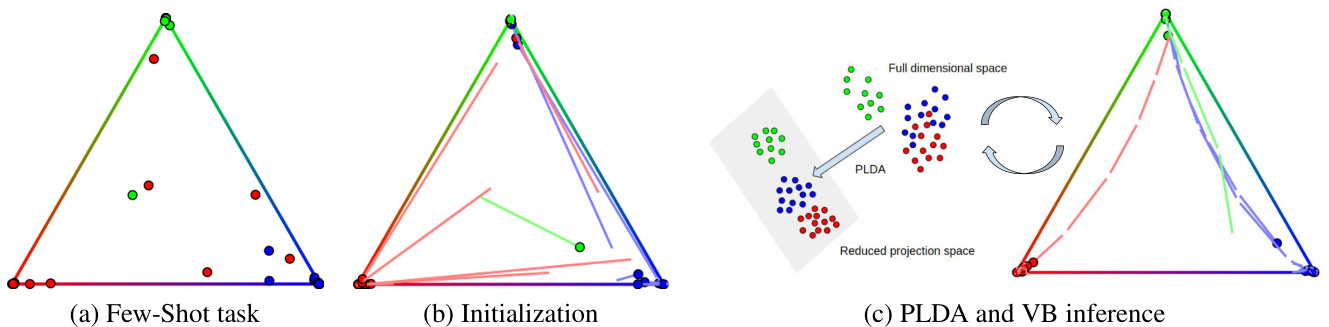
Figure 1: Summary of the proposed method. Here we illustrate a 3-way classification task in a standard 2-simplex using soft-classification probabilities. Trajectories show the evolution across iterations. For a given Few-Shot task which nearest-class-mean probabilities are depicted in (a), a Soft-KMEANS clustering method is performed in (b) to initialize $O_{n k}$ (see Alg. 1). Then in (c) an iterative ly refined Variation al Bayesian (VB) model with Adaptive Dimension Reduction using Probabilistic Linear Discriminant Analysis (PLDA) is applied to obtain the final class predictions.
图 1: 所提方法概述。这里我们使用软分类概率在标准2-单纯形中展示了一个三分类任务。轨迹线显示了迭代过程中的演化过程。对于给定的少样本任务,其最近类均值概率如(a)所示,(b)中执行了Soft-KMEANS聚类方法以初始化$O_{n k}$(参见算法1)。然后在(c)中应用了基于概率线性判别分析(PLDA)的自适应降维变分贝叶斯(VB)模型进行迭代优化,最终获得类别预测结果。
This limitation of benchmarking for trans duct ive FSC has recently been discussed in [39]. In this paper, the authors propose a new way of generating trans duct ive FSC benchmarks where the distribution of samples among classes can drastically change from a Few-Shot generated task to the next one. Interestingly, they showed the impact of generating class imbalance on the performance on various popular methods, resulting in some cases in drops in average accuracy of more than $10%$ .
[39] 近期讨论了转导式小样本分类 (transductive FSC) 基准测试的这一局限性。该论文提出了一种新的转导式小样本分类基准生成方法,其类别样本分布可能在相邻少样本生成任务间发生剧烈变化。值得注意的是,他们揭示了类别不平衡生成对多种主流方法性能的影响,某些情况下平均准确率降幅超过 $10%$。
A simple way to reach state-of-the-art performance in trans duct ive FSC consists in extracting features from the available samples using a pretrained backbone deep learning architecture, and then using semi-supervised clustering routines to estimate samples distribution among classes. Due to the very limited number of available samples, distribution-agnostic clustering algorithms are often preferred, such as K-MEANS or its variants [29, 25, 32] or mean-shift [9] for instance.
在传导式少样本分类 (FSC) 中实现最先进性能的简单方法是:使用预训练的骨干深度学习架构从可用样本中提取特征,然后通过半监督聚类流程估算样本的类别分布。由于可用样本数量极少,通常优先选择与分布无关的聚类算法,例如 K-MEANS 及其变体 [29, 25, 32] 或均值漂移 [9]。
In this paper, we are interested in showing it is possible to combine data reduction with statistical inference through a Variation al Bayesian (VB) [13] approach. Here, data reduction helps considerably reduce the number of parameters to infer, while VB provides more flexibility than the usual K-Means methods. Interestingly, the proposed approach can easily cope with standard e qui distributed Few-Shot tasks or the unbalanced ones proposed in [39], defining a new state-of-the-art for five popular trans duct ive Few-Shot vision classification benchmarks.
本文旨在证明通过变分贝叶斯 (Variational Bayesian, VB) [13] 方法将数据降维与统计推断相结合的可能性。数据降维能显著减少待推断参数数量,而VB方法相比传统K-Means具有更高灵活性。值得注意的是,该方法不仅能处理标准均匀分布的少样本任务,还能应对[39]提出的非均衡任务,在五个主流转导式少样本视觉分类基准测试中创造了新的最优性能。
Our claims are the following:
我们的主张如下:
2 Related work
2 相关工作
There are two main frameworks in the field of FSC: 1) only one unlabelled sample is processed at a time for class predictions, which is called inductive FSC, and 2) the entire unlabelled samples are available for further estimations, which is called trans duct ive FSC. Inductive methods focus on training a feature extractor that generalizes well the embedding in a feature sub-space, they include meta learning methods such as [12, 26, 2, 40, 30, 37] that train a model in an episodic manner, and transfer learning methods [8, 28, 48, 5, 3, 33] that train a model with a set of mini-batches. Recent state-of-the-art works on inductive FSC [46, 47, 43, 19] combine the above two strategies and propose a transfer based training used as model initialization, followed by an episodic training that adapts the model to better fit the Few-Shot tasks.
FSC领域主要有两种框架:1) 每次仅处理一个未标记样本进行类别预测,称为归纳式FSC (inductive FSC);2) 所有未标记样本均可用于进一步估计,称为直推式FSC (transductive FSC)。归纳方法侧重于训练能在特征子空间中良好泛化嵌入的特征提取器,包括以情景化方式训练模型的元学习方法 [12, 26, 2, 40, 30, 37],以及通过小批量集训练模型的迁移学习方法 [8, 28, 48, 5, 3, 33]。近期最先进的归纳式FSC研究 [46, 47, 43, 19] 结合了上述两种策略,提出先采用基于迁移的训练进行模型初始化,再通过情景化训练使模型更好地适应少样本任务。
Trans duct ive methods are becoming more and more popular thanks to their better performance due to the use of unlabelled data, as well as their utility in situations where data annotation is costly. Early literature of this branch operates on a class-balanced setting where unlabelled instances are evenly distributed among targeted classes. Graphbased methods [14, 7, 44, 21] make use of the affinity among features and propose to group those that belong to the same class. More recent works such as [16] propose methods based on Optimal Transport that realizes sample-class allocation with a minimum cost. While effective, these methods often require class-balanced priors to work well, which is not realistic due to the arbitrary unknown query set. In [39] the authors put forward a novel unbalanced setting that composes a query set with unlabelled instances sampled following a Dirichlet distribution, injecting more imbalance for predictions.
转导式方法因其利用未标注数据带来更优性能,以及在数据标注成本高昂场景中的实用性而日益流行。该分支的早期研究基于类别平衡设定,即未标注实例均匀分布于目标类别间。基于图的方法 [14, 7, 44, 21] 利用特征间相似性,提出将同类样本归组的策略。[16] 等最新研究则提出基于最优传输 (Optimal Transport) 的方法,以最小成本实现样本-类别分配。尽管有效,这些方法通常依赖类别平衡先验才能良好运作,而实际场景中未知查询集的任意性使得该假设不成立。[39] 提出了一种新型非平衡设定,通过狄利克雷分布 (Dirichlet distribution) 采样构建查询集,为预测注入更强不平衡性。
In this paper we propose a clustering method to solve trans duct ive FSC, where the aim is to estimate cluster parameters giving high predictions for unlabelled samples. Under Gaussian assumptions, previous works [25, 32] have utilised algorithms such as Expectation Maximization [10] (EM), with the goal of maximizing likelihoods or posteriors with respect to the parameters for a cluster, with the hidden variables marginalized. However, this may not be the most suitable way due to the scarcity of available data in a given Few-Shot task, which increases the level of uncertainty for cluster estimations. Therefore, in this paper we propose a Variation al Bayesian (VB) approach, in which we regard some unknown parameters as hidden variables in order to inject more flexibility into the model, and we try to approximate the posterior of the hidden variables by a variation al distribution.
本文提出一种聚类方法来解决直推式少样本分类问题,其目标是通过估计聚类参数来对未标记样本进行高准确率预测。在高斯分布假设下,先前研究[25, 32]采用期望最大化算法[10] (EM),通过边缘化隐变量来最大化关于聚类参数的似然或后验概率。然而在少样本任务中,由于可用数据稀缺会增大聚类估计的不确定性,这种方法可能并非最优解。因此,本文提出变分贝叶斯(VB)方法,将部分未知参数视为隐变量以增强模型灵活性,并通过变分分布来近似隐变量的后验概率。
As models with too few labelled samples often give too much randomness for a cluster to be stably reckoned, they often require the use of feature dimension reduction techniques to stabilize cluster estimations. Previous literature such as [25] applies a PCA method that reduces dimension in a non-supervised manner, and [6] proposes a modified LDA during backbone training that maximizes the ratio of inter/intra-class distance. In this paper we propose to use Probabilistic Linear Discriminant Analysis [17] (PLDA) that 1) is applied on extracted features, 2) fits data more desirably into distribution assumptions, and 3) is semi-supervised in combination of a VB model. We integrate PLDA into the VB model in order to refine the reduced space through iterations.
由于标注样本过少的模型往往会给聚类带来过多随机性而难以稳定计算,通常需要使用特征降维技术来稳定聚类估计。先前文献如[25]采用了一种无监督降维的PCA方法,而[6]则在骨干网络训练过程中提出改进的LDA以最大化类间/类内距离比。本文提出采用概率线性判别分析[17](PLDA),其特点在于:1) 作用于提取后的特征;2) 使数据更符合分布假设;3) 与VB模型结合形成半监督框架。我们将PLDA集成到VB模型中,通过迭代优化降维空间。
3 Methodology
3 方法论
In this section, we firstly present the standard setting in trans duct ive FSC, including the latest unbalanced setting proposed by [39] where unlabelled samples are non-uniformly distributed among classes. Then we present our proposed method combining PLDA and VB inference.
在本节中,我们首先介绍转导式小样本分类 (FSC) 的标准设置,包括[39]提出的最新非均衡设置 (unbalanced setting) ,其中未标记样本在类别间呈非均匀分布。随后介绍我们提出的结合PLDA与VB推断的方法。
3.1 Problem formulation
3.1 问题表述
Following other works in the domain, our proposed method is operated on a feature space obtained from a pre-trained backbone. Namely, we are given the extracted features of 1) a generic base class dataset $\mathcal{D}{b a s e}={\pmb{x}{i}^{b a s e}}{i=1}^{N_{b a s e}}\in\mathcal{C}{b a s e}$ that contains $N_{b a s e}$ labelled samples where each sample $\pmb{x}{i}^{b a s e}$ is a column vector of length $D$ , and $\mathcal{C}{b a s e}$ is the set of base classes to which these samples belong. These base classes have been used to train the backbone. And similarly, 2) a novel class dataset $\mathcal{D}{n o v e l}\overset{\cdot}{=}{\pmb{x}{n}^{n o v e l}}{n=1}^{N}$ containing $N$ samples belonging to a set of $K$ novel classes $\mathcal{C}{n o v e l}$ $(\mathcal{C}{b a s e}\cap\mathcal{C}{n o v e l}=\emptyset)$ . On this novel dataset, only a few elements are labelled, and the aim is to predict the missing labels. Denote X the matrix obtained by aggregating elements in $\mathcal{D}_{n o v e l}$ row-wise.
遵循该领域的其他工作,我们提出的方法在一个通过预训练骨干网络获取的特征空间上运行。具体而言,我们获得了以下两种提取特征:1) 通用基类数据集 $\mathcal{D}{b a s e}={\pmb{x}{i}^{b a s e}}{i=1}^{N_{b a s e}}\in\mathcal{C}{b a s e}$,其中包含 $N_{b a s e}$ 个带标签样本,每个样本 $\pmb{x}{i}^{b a s e}$ 是一个长度为 $D$ 的列向量,$\mathcal{C}{b a s e}$ 是这些样本所属的基类集合。这些基类已用于训练骨干网络。类似地,2) 新类数据集 $\mathcal{D}{n o v e l}\overset{\cdot}{=}{\pmb{x}{n}^{n o v e l}}{n=1}^{N}$ 包含 $N$ 个样本,属于 $K$ 个新类 $\mathcal{C}{n o v e l}$ $(\mathcal{C}{b a s e}\cap\mathcal{C}{n o v e l}=\emptyset)$。在这个新数据集上,只有少数元素被标记,目标是预测缺失的标签。将 $\mathcal{D}_{n o v e l}$ 中的元素按行聚合得到的矩阵记为 X。
When benchmarking trans duct ive FSC methods, it is common to randomly generate Few-Shot tasks by sampling $\mathcal{D}{n o v e l}$ from a larger dataset. These tasks are generated by sampling $K$ distinct classes, $L$ distinct labelled elements for each class (called support set) and $Q$ total unlabelled elements without repetition and distinct from the labelled ones (called query set). All these unlabelled elements belong to one of the selected classes. We obtain a total of $N=K L+Q$ elements in the task, and compute the accuracy on the $Q$ unlabelled ones. Depending on how unlabelled instances are distributed among selected classes within a task, we further distinguish a balanced setting where the query set is evenly distributed among the $K$ classes, from an unbalanced setting where it can vary from class to class. An automatic way to generate such unbalanced Few-Shot tasks has been proposed in [39] where the number of elements to draw from each class is determined using a Dirichlet distribution parameterized by $\alpha_{o}^{*}\mathbf{1}$ , where 1 is the all-one vector. To solve a trans duct ive FSC task, our method is composed of PLDA and VB inference, that we introduce in the next paragraphs.
在对转导式少样本分类 (FSC) 方法进行基准测试时,通常的做法是从更大的数据集中采样 $\mathcal{D}{n o v e l}$ 来随机生成少样本任务。这些任务通过采样 $K$ 个不同类别、每个类别 $L$ 个不同的带标签元素(称为支持集)以及 $Q$ 个不带标签且与带标签元素不重复的总元素(称为查询集)来生成。所有这些不带标签的元素都属于所选类别之一。我们在任务中总共获得 $N=K L+Q$ 个元素,并在 $Q$ 个不带标签的元素上计算准确率。根据不带标签的实例在任务中选定的类别之间的分布情况,我们进一步区分了查询集在 $K$ 个类别之间均匀分布的平衡设置,以及在不同类别之间可能有所变化的不平衡设置。[39] 中提出了一种自动生成这种不平衡少样本任务的方法,其中从每个类别抽取的元素数量由参数化为 $\alpha_{o}^{*}\mathbf{1}$ 的狄利克雷分布确定,其中 1 是全 1 向量。为了解决转导式 FSC 任务,我们的方法由 PLDA 和 VB 推断组成,我们将在接下来的段落中介绍。
3.2 Probabilistic Linear Discriminant Analysis (PLDA)
3.2 概率线性判别分析 (PLDA)
In our work, PLDA [17] is mainly used to reduce feature dimensions. For a Few-Shot task $\mathbf{X}$ , let $\Phi_{w}$ be a positive definite matrix representing the estimated shared within-class covariance of a given class, and $\Phi_{b}$ be a positive semidefinite matrix representing the estimated between-class covariance that generates class variables. The goal of PLDA is to project data onto a subspace while maximizing the signal-to-noise ratio for class labelling. In details, we obtain a projection matrix W that diagonal ize s both $\Phi_{w}$ and $\Phi_{b}$ and yield the following equations:
在我们的工作中,PLDA [17] 主要用于降低特征维度。对于一个少样本任务 $\mathbf{X}$,设 $\Phi_{w}$ 为表示给定类别的估计共享类内协方差的正定矩阵,$\Phi_{b}$ 为表示生成类别变量的估计类间协方差的半正定矩阵。PLDA 的目标是将数据投影到一个子空间,同时最大化类别标记的信噪比。具体而言,我们得到一个对角化 $\Phi_{w}$ 和 $\Phi_{b}$ 的投影矩阵 W,并得到以下方程:
$$
\mathbf{W}^{T}\mathbf{\Phi}\mathbf{\Phi}{w}\mathbf{W}=\mathbf{I},\quad\mathbf{W}^{T}\mathbf{\Phi}\mathbf{\Phi}_{b}\mathbf{W}=\boldsymbol{\Psi}
$$
$$
\mathbf{W}^{T}\mathbf{\Phi}\mathbf{\Phi}{w}\mathbf{W}=\mathbf{I},\quad\mathbf{W}^{T}\mathbf{\Phi}\mathbf{\Phi}_{b}\mathbf{W}=\boldsymbol{\Psi}
$$
where I is an identity matrix and $\Psi$ is a diagonal matrix. In this paper, we assume a similar distribution between the pre-trained base classes and the transferred novel classes [45]. Therefore we propose to estimate $\Phi_{w}$ to be the within-class scatter matrix of $\mathcal{D}{b a s e}$ , denoted as $\mathbf{S}{w}^{b a s s}$ . In practice we implement PLDA by firstly transforming $\mathbf{X}$ using a rotation matrix $\mathbf{R}\in\mathbb{R}^{D\times D}$ and a set of scaling values $\pmb{s}\in\mathbb{R}^{D}$ obtained from $\mathbf{S}{w}^{b a s e}$ . Note that we clamp the scaling values to be no larger than an upper-bound $s_{m a x}$ in order to prevent too large values, $s_{m a x}$ is a hyper-parameter. Then we project the transformed data onto their estimated class centroids space, in accordance with the $d$ largest eigenvalues of $\Psi$ , and obtain dimension-reduced data ${\bf U}=[{\pmb u}{1},...,{\pmb u}{n},...,{\pmb u}{N}]^{\dot{T}}\in\mathbb{R}^{N\times d}$ where $\pmb{u}{n}=\mathbf{W}^{T}\pmb{x}_{n}$ and $d=K-1$ More detailed implementation can be found in Appendix.
其中 I 是单位矩阵,$\Psi$ 是对角矩阵。本文假设预训练基类与迁移新类具有相似分布 [45],因此我们提出将 $\Phi_{w}$ 估计为 $\mathcal{D}{base}$ 的类内散布矩阵,记作 $\mathbf{S}{w}^{base}$。实际实现PLDA时,首先通过旋转矩阵 $\mathbf{R}\in\mathbb{R}^{D\times D}$ 和从 $\mathbf{S}{w}^{base}$ 获取的缩放值 $\pmb{s}\in\mathbb{R}^{D}$ 对 $\mathbf{X}$ 进行变换。为防止数值过大,我们将缩放值限制在上限 $s_{max}$ 内(该值为超参数)。随后根据 $\Psi$ 的 $d$ 个最大特征值,将变换后的数据投影至估计的类质心空间,得到降维数据 ${\bf U}=[{\pmb u}{1},...,{\pmb u}{n},...,{\pmb u}{N}]^{\dot{T}}\in\mathbb{R}^{N\times d}$,其中 $\pmb{u}{n}=\mathbf{W}^{T}\pmb{x}_{n}$ 且 $d=K-1$。完整实现详见附录。
3.3 Variation al Bayesian (VB) Inference
3.3 变分贝叶斯 (Variational Bayesian, VB) 推断
During VB inference, we operate on a reduced $d$ -dimensional space obtained after applying PLDA. Considering a Gaussian mixture model for a given task ${\bf U}\in\mathbb{R}^{N\times d}$ in reduced space, let $\theta$ be the unknown variables of the model. In VB we attempt to find a probability distribution $q(\theta)$ that approximates the true posterior $p(\boldsymbol{\theta}|\mathbf{U})$ , i.e. maximizes the ELBO (see Appendix for more details). In our case, we define $\theta={Z,\pi,\mu}$ where $Z={z_{n}}{n=1}^{N}$ is a set of latent variables used as class indicators, each latent variable has an one-of-K representation, $\pi$ is a $K$ -dimensional vector representing mixing ratios between the classes, and $\pmb{\mu}={\pmb{\mu}{k}}{k=1}^{K}$ where $\pmb{\mu}{k}$ is the centroid for class $k$ . Note that 1) contrary to EM where $\pi,\mu$ are seen as parameters that can be estimated directly, in VB they are deemed as hidden variables following certain distribution laws. 2) This is not a full VB model due to the lack of precision matrix (i.e. the inverse of covariance matrix) as a variable in $\theta$ . Although a VB model frees up more parameters for the unknown variables, it also increases the instability in estimations so that the model becomes too sensible. Therefore, in this paper we impose an assumption that all classes in $\mathbf{U}$ share the same precision matrix and it is fixed during VB iterations. Namely we define $\mathbf{\Lambda}{\mathbf{{\Lambda}}{k}}=\mathbf{\Lambda}{\mathbf{{\Lambda}}}={\mathit{T}}{v b}\mathbf{I}$ for $k=1,...,K$ , where $T_{v b}$ is a hyper-parameter in order to compensate the variation between base and estimated novel class distributions.
在VB (Variational Bayes) 推理过程中,我们在应用PLDA后获得的降维 $d$ 维空间中进行操作。考虑降维空间中给定任务 ${\bf U}\in\mathbb{R}^{N\times d}$ 的高斯混合模型,设 $\theta$ 为模型的未知变量。在VB中,我们试图找到一个近似真实后验 $p(\boldsymbol{\theta}|\mathbf{U})$ 的概率分布 $q(\theta)$ ,即最大化ELBO (详见附录)。在本研究中,我们定义 $\theta={Z,\pi,\mu}$ ,其中 $Z={z_{n}}{n=1}^{N}$ 是作为类别指示符的潜变量集合,每个潜变量采用one-of-K表示法, $\pi$ 是表示类别混合比例的 $K$ 维向量, $\pmb{\mu}={\pmb{\mu}{k}}{k=1}^{K}$ 其中 $\pmb{\mu}{k}$ 是类别 $k$ 的质心。需要注意的是:1) 与EM算法将 $\pi,\mu$ 视为可直接估计的参数不同,在VB中它们被视为遵循特定分布规律的隐变量;2) 由于 $\theta$ 中缺少精度矩阵 (即协方差矩阵的逆) 作为变量,这不是一个完整的VB模型。虽然VB模型为未知变量释放了更多参数,但也增加了估计的不稳定性,使得模型过于敏感。因此,本文假设 $\mathbf{U}$ 中所有类别共享相同的精度矩阵,并在VB迭代过程中保持固定。具体定义为 $\mathbf{\Lambda}{\mathbf{{\Lambda}}{k}}=\mathbf{\Lambda}{\mathbf{{\Lambda}}}={\mathit{T}}{v b}\mathbf{I}$ ( $k=1,...,K$ ),其中超参数 $T_{v b}$ 用于补偿基础类别分布与估计新类别分布之间的差异。
In order for a model to be in a variation al bayesian setting, we define priors and likelihoods on the unknown variables, with several initialization parameters attached:
为了使模型处于变分贝叶斯 (variational bayesian) 设定中,我们在未知变量上定义先验和似然函数,并附带若干初始化参数:
$$
\begin{array}{r l}{{\mathrm{priors:}}}&{{p(\pi)=D i r(\pi|\alpha_{o}),\quad p(\mu)=\displaystyle\prod_{k=1}^{K}\mathcal{N}(\mu_{k}|m_{o},(\beta_{o}\Lambda)^{-1}),}}\ {{\mathrm{likelihoods:}}}&{{p(Z|\pi)=\displaystyle\prod_{n=1}^{N}C a t e g o r i c a l(z_{n}|\pi),\quad p(U|Z,\mu)=\displaystyle\prod_{n=1}^{N}\displaystyle\prod_{k=1}^{K}\mathcal{N}(u_{n}|\mu_{k},\Lambda^{-1})^{z_{n k}}}}\end{array}
$$
$$
\begin{array}{r l}{{\mathrm{先验分布:}}}&{{p(\pi)=D i r(\pi|\alpha_{o}),\quad p(\mu)=\displaystyle\prod_{k=1}^{K}\mathcal{N}(\mu_{k}|m_{o},(\beta_{o}\Lambda)^{-1}),}}\ {{\mathrm{似然函数:}}}&{{p(Z|\pi)=\displaystyle\prod_{n=1}^{N}C a t e g o r i c a l(z_{n}|\pi),\quad p(U|Z,\mu)=\displaystyle\prod_{n=1}^{N}\displaystyle\prod_{k=1}^{K}\mathcal{N}(u_{n}|\mu_{k},\Lambda^{-1})^{z_{n k}}}}\end{array}
$$
where $\pi$ follows a K-dimensional symmetric Dirichlet distribution, with $\alpha_{o}$ being the prior of component weight for each class, which we set to 2.0 in accordance with [39], i.e. the same value as the Dirichlet distribution parameter $\alpha_{o}^{*}$ that is used to generate Few-Shot tasks. The vector $m_{o}$ is the prior about the class centroid variables, we let it to be 0. And $\beta_{o}$ stands for the prior about the moving range of class centroid variables: the larger it is, the closer the centroids are to $m_{o}$ . We empirically found that $\beta_{o}=10.0$ gives consistent good results across datasets and FSC problems.
其中 $\pi$ 服从 K 维对称狄利克雷分布 (Dirichlet distribution),$\alpha_{o}$ 作为每个类别的分量权重先验,我们按照 [39] 将其设为 2.0,即与生成少样本任务时使用的狄利克雷分布参数 $\alpha_{o}^{*}$ 相同。向量 $m_{o}$ 是类别中心变量的先验,我们设其为 0。$\beta_{o}$ 表示类别中心变量移动范围的先验:该值越大,中心点越接近 $m_{o}$。我们通过实验发现 $\beta_{o}=10.0$ 能在不同数据集和少样本分类问题上取得稳定良好的结果。
As previously stated, we approximate a variable distribution to the true posterior. To further simplify, we follow the Mean-Field assumption [31, 18] and assume that the unknown variables are independent from one another. Therefore we let $q(\theta)=q(\bar{Z},\pi,\mu)=q(Z)q(\pi)q(\mu)\approx p(Z,\pi,\mu/\mathbf{U})$ and solve for each term. The explicit formulation for these marginals is provided in Eq. 3, 4 (see Appendix for more details). The estimation of the various parameters is then classically performed through an iterative EM framework as presented further.
如前所述,我们用一个变量分布来近似真实后验。为了进一步简化,我们遵循平均场假设 [31, 18] ,并假设未知变量彼此独立。因此,我们设 $q(\theta)=q(\bar{Z},\pi,\mu)=q(Z)q(\pi)q(\mu)\approx p(Z,\pi,\mu/\mathbf{U})$ ,并对每一项求解。这些边缘分布的具体表达式见公式3、4(更多细节见附录)。随后,通过一个迭代的EM框架对各个参数进行经典估计,如下所述。
Denote $\pmb{o}{n}=[o_{n1},...,o_{n k},...,o_{n K}]$ as the soft class assignment for ${\pmb u}{n}$ $\left(o_{n k}\ge0\right.$ , $\begin{array}{r}{\sum_{k=1}^{K}o_{n k}=1,}\end{array}$ , and $o_{n k}$ represents the portion of nth sample allocated to $k$ th class.
记 $\pmb{o}{n}=[o_{n1},...,o_{n k},...,o_{n K}]$ 为 ${\pmb u}{n}$ 的软类别分配 (其中 $o_{n k}\ge0$ , $\begin{array}{r}{\sum_{k=1}^{K}o_{n k}=1,}\end{array}$ ,且 $o_{n k}$ 表示第 $n$ 个样本分配给第 $k$ 个类别的比例)。
M step: In this step we estimate $q(\pi)$ and $q({\pmb\mu})$ in use of the class assignments $O_{n k}$ :
M步:在此步骤中,我们利用类别分配 $O_{n k}$ 来估计 $q(\pi)$ 和 $q({\pmb\mu})$:
$$
p(\pmb{\pi})=D i r(\pmb{\pi})\implies q^{*}(\pmb{\pi})=D i r(\pmb{\pi}|\alpha)\quad\mathrm{with}\quad\alpha_{k}=\alpha_{o}+N_{k},
$$
$$
p(\pmb{\pi})=D i r(\pmb{\pi})\implies q^{*}(\pmb{\pi})=D i r(\pmb{\pi}|\alpha)\quad\mathrm{with}\quad\alpha_{k}=\alpha_{o}+N_{k},
$$
twhhe esroe $\pmb{\alpha}=[\alpha_{1},...,\alpha_{k},...,\alpha_{K}]$ palree st ihne celsatsism .t edW ec oalmsop oensteinmt awtee itghhe tsm foovri nclga rsasnesg,e apnadr $\begin{array}{r}{N_{k}=\sum_{n=1}^{N}o_{n k}}\end{array}$ ics etnhter osiud $k$ $\beta_{k}$ $m_{k}$ for each class centroid variable. We observe that the posteriors take the same forms as the priors. Demonstration of these results is presented in Appendix.
规则:
- 输出中文翻译部分时,仅保留翻译标题,无冗余内容、无重复、无解释。
- 不输出无关内容。
- 保留原始段落格式及术语(如FLAC、JPEG)、公司缩写(如Microsoft、Amazon、OpenAI)。
- 人名不译。
- 保留文献引用格式(如[20])。
- Figure/Table翻译保留原格式(如"图1: "、"表1: ")。
- 全角括号转半角,并添加半角空格(如"(Generative AI)"→" (Generative AI)")。
- 专业术语首次出现标注英文(如"生成式AI (Generative AI)"),后续直接使用中文。
- AI术语对照:
- Transformer→Transformer
- Token→Token
- LLM→大语言模型
- Zero-shot→零样本
- Few-shot→少样本
- AI Agent→AI智能体
- AGI→通用人工智能
- Python→Python语言
策略:
- 特殊字符/公式原样保留
- HTML表格转Markdown格式
- 准确翻译并符合中文表达习惯
最终仅返回Markdown格式译文,无无关内容。
$\mathbf{E}$ step: In this step we estimate $q(Z)$ by updating $o_{n k}$ , using the current values of all other parameters computed in the M-step, i.e. $\alpha_{k},\beta_{k}$ and $\mathbf{\nabla}m_{k}$ .
$\mathbf{E}$ 步:在此步骤中,我们通过更新 $o_{n k}$ 来估计 $q(Z)$,使用在 M 步中计算的所有其他参数的当前值,即 $\alpha_{k}$、$\beta_{k}$ 和 $\mathbf{\nabla}m_{k}$。
$$
p(Z|\pi)=\prod_{n=1}^{N}C a t e g o r i c a l(z_{n}|\pi)\implies q^{*}(Z)=\prod_{n=1}^{N}C a t e g o r i c a l(z_{n}|\sigma_{n})
$$
$$
p(Z|\pi)=\prod_{n=1}^{N}C a t e g o r i c a l(z_{n}|\pi)\implies q^{*}(Z)=\prod_{n=1}^{N}C a t e g o r i c a l(z_{n}|\sigma_{n})
$$
where each element $o_{n k}$ can be computed as $\begin{array}{r}{o_{n k}=\frac{\rho_{n k}}{\sum_{j=1}^{K}\rho_{n j}}}\end{array}$ in which:
其中每个元素 $o_{n k}$ 可计算为 $\begin{array}{r}{o_{n k}=\frac{\rho_{n k}}{\sum_{j=1}^{K}\rho_{n j}}}\end{array}$ ,其中:
$$
\log\rho_{n k}=\psi(\alpha_{k})-\psi(\sum_{j=1}^{K}\alpha_{j})+\frac{1}{2}\log|\mathbf{A}|-\frac{d}{2}\log2\pi-\frac{1}{2}[d\beta_{k}^{-1}+(u_{n}-m_{k})^{T}\mathbf{A}(u_{n}-m_{k})],
$$
$$
\log\rho_{n k}=\psi(\alpha_{k})-\psi(\sum_{j=1}^{K}\alpha_{j})+\frac{1}{2}\log|\mathbf{A}|-\frac{d}{2}\log2\pi-\frac{1}{2}[d\beta_{k}^{-1}+(u_{n}-m_{k})^{T}\mathbf{A}(u_{n}-m_{k})],
$$
with $\psi(\cdot)$ being the logarithmic derivative of the gamma function (also known as the digamma function). We observe that $q^{*}(Z)$ follows the same categorical distribution as the likelihood, and it is parameterized by $o_{n k}$ . More details can be found in Appendix.
其中 $\psi(\cdot)$ 是伽玛函数的对数导数(也称为digamma函数)。我们观察到 $q^{*}(Z)$ 遵循与似然相同的分类分布,并由 $o_{n k}$ 参数化。更多细节见附录。
Proposed algorithm The proposed method combines PLDA and VB inference which leads to an Efficiency Guided Adaptive Dimension Reduction for VAriation al BAyesian inference. We thus name our proposed method “BAVARDAGE”, and the detailed description is presented in Algorithm 1. Given a Few-Shot task X and a within-class scatter matrix $\mathbf{S}{w}^{b a s e}$ , we initialize $o_{n k}$ using EM algorithm with an assumed covariance matrix, adjusted by a temperature hyper-parameter $T_{k m}$ , for all classes. Note that this is equivalent to Soft-KMEANS [20] algorithm. And for each iteration we update parameters: in $\mathbf{M}$ step we update $\alpha_{k},\beta_{k}$ and centroids $m_{k}$ , in E step we only update $o_{n k}$ , and we apply PLDA with the updated $o_{n k}$ to reduce feature dimensions. Finally, predicted labels are obtained by selecting the class that corresponds to the largest value in $O_{n k}$ .
提出的算法
该方法结合了PLDA和VB推断,实现了针对变分贝叶斯推断的高效引导自适应降维。因此,我们将提出的方法命名为“BAVARDAGE”,其详细描述如算法1所示。给定一个少样本任务X和类内散度矩阵$\mathbf{S}{w}^{b a s e}$,我们使用EM算法初始化$o_{n k}$,并假设一个协方差矩阵,通过温度超参数$T_{k m}$对所有类别进行调整。注意,这等价于Soft-KMEANS [20]算法。在每次迭代中,我们更新参数:在$\mathbf{M}$步中更新$\alpha_{k},\beta_{k}$和质心$m_{k}$,在E步中仅更新$o_{n k}$,并利用更新后的$o_{n k}$应用PLDA进行特征降维。最终,通过选择$O_{n k}$中最大值对应的类别获得预测标签。
The illustration of our proposed method is presented in Figure 1. For a Few-Shot task that has three classes (red, blue and green) with unlabelled samples depicted on the probability simplex, we firstly initialize $O_{n k}$ with Soft-KMEANS which directs some data points to their belonging classes while further distancing some points from their targeted classes. Then we apply the proposed VB inference integrated with PLDA, resulting in additional points moving towards their corresponding classes.
我们提出的方法如图 1 所示。对于一个包含三个类别 (红色、蓝色和绿色) 且未标记样本在概率单纯形上表示的少样本任务,我们首先用 Soft-KMEANS 初始化 $O_{n k}$ ,这会使部分数据点指向其所属类别,同时使另一些点远离目标类别。然后我们应用提出的结合 PLDA 的 VB (Variational Bayesian) 推断,使得更多点向对应类别移动。
4 Experiments
4 实验
In this section we provide details on the standard trans duct ive Few-Shot classification settings, and we evaluate the performance of our proposed method.
在本节中,我们将详细介绍标准的转导式少样本分类设置,并评估所提出方法的性能。
Benchmarks We test our method on standard Few-Shot benchmarks: mini-Imagenet [35], tiered-Imagenet [32] and caltech-ucsd birds-200-2011 (CUB) [41]. mini-Imagenet is a subset of ILSVRC-12 [35] dataset, it contains a total of 60, 000 images of size $84\times84$ belonging to 100 classes (600 images per class) and follows a 64-16-20 split for base, validation and novel classes. tiered-Imagenet is a larger subset of ILSVRC-12 containing 608 classes with 779, 165 images of size $84\times84$ in total, and we use the standard 351-97-160 split, and CUB is composed of 200 classes following a 100-50-50 split (Image size: $84\times84$ ). In Appendix we also show the performance of our proposed method on other well-known Few-Shot benchmarks such as FC100 [30] and CIFAR-FS [4].
基准测试
我们在标准少样本基准测试上验证了方法性能:mini-Imagenet [35]、tiered-Imagenet [32] 和 caltech-ucsd birds-200-2011 (CUB) [41]。mini-Imagenet 是 ILSVRC-12 [35] 数据集的子集,包含 100 个类别的 60,000 张 $84\times84$ 尺寸图像(每类 600 张),按 64-16-20 划分基础类、验证类和新类。tiered-Imagenet 是更大的 ILSVRC-12 子集,涵盖 608 个类别共 779,165 张 $84\times84$ 图像,采用标准 351-97-160 划分。CUB 数据集包含 200 个类别,按 100-50-50 划分(图像尺寸:$84\times84$)。附录中还展示了该方法在 FC100 [30] 和 CIFAR-FS [4] 等其他知名少样本基准的表现。
Algorithm 1 BAVARDAGE
算法 1 BAVARDAGE
Settings Following previous works [25, 34, 39], our proposed method is evaluated on 1-shot 5-way ( $K=5$ , $L=1$ ), and 5-shot 5-way $K=5$ , $L=5$ ) scenarios. As for the query set, we set a total number of $Q=75$ unlabelled samples, from which we further define two settings: 1) a balanced setting where unlabelled instances are evenly distributed among $K$ classes, and 2) an unbalanced setting where the query set is randomly distributed, following a Dirichlet distribution parameterized by $\alpha_{o}^{}$ . In our paper we follow the same setting as [39] and set $\alpha_{o}^{*}=2.0$ , further experiments with different values are conducted in the next sections. The performance of our proposed method is evaluated by computing the averaged accuracy over 10, 000 Few-Shot tasks.
设置
遵循先前的工作 [25, 34, 39],我们提出的方法在 1-shot 5-way ( $K=5$ , $L=1$ ) 和 5-shot 5-way ( $K=5$ , $L=5$ ) 场景下进行评估。对于查询集,我们设置了总共 $Q=75$ 个未标记样本,并进一步定义两种设置:1) 平衡设置,其中未标记实例均匀分布在 $K$ 个类别中;2) 不平衡设置,其中查询集随机分布,遵循由 $\alpha_{o}^{}$ 参数化的狄利克雷分布。在本文中,我们采用与 [39] 相同的设置,设定 $\alpha_{o}^{*}=2.0$,不同值的进一步实验将在后续章节中进行。我们通过计算 10,000 个少样本任务的平均准确率来评估所提方法的性能。
Implementation details In this paper we firstly compare our proposed algorithm with the other state-of-the-art methods using the same pretrained backbones and benchmarks provided in [39]. Namely we extract the features using the same ResNet-18 (RN18) and Wide Res Net 28 10 (WRN) neural models, and present the performance on mini-Imagenet, tiered-Imagenet and CUB datasets. In our proposed method, the raw features are pre processed following [42]. As for the hyper-parameters, we set $T_{k m}=10,T_{v b}=50,s_{m a x}=2$ for the balanced setting; $T_{k m}=50,T_{v b}=50,s_{m a x}=1$ for the unbalanced setting, and we use the same VB priors for all settings. To further show the functionality of our proposed method on different backbones and other benchmarks, we tested BAVARDAGE on a recent high performing feature extractor trained on a ResNet-12 (RN12) neural model [28, 3], and we report the accuracy in Table 1 and in Appendix with various settings.
实现细节
本文首先将我们提出的算法与[39]中提供的其他最先进方法进行比较,使用相同的预训练主干网络和基准测试。具体而言,我们使用相同的ResNet-18 (RN18)和Wide ResNet-28-10 (WRN)神经网络模型提取特征,并在mini-Imagenet、tiered-Imagenet和CUB数据集上展示性能。在我们的方法中,原始特征按照[42]的方式进行预处理。关于超参数,平衡设置下设为$T_{km}=10,T_{vb}=50,s_{max}=2$;非平衡设置下设为$T_{km}=50,T_{vb}=50,s_{max}=1$,且所有设置均采用相同的VB先验。为了进一步展示所提方法在不同主干网络和其他基准测试上的功能,我们在基于ResNet-12 (RN12)神经网络模型[28,3]训练的最新高性能特征提取器上测试了BAVARDAGE,并在表1和附录中报告了多种设置下的准确率。
4.1 Main results
4.1 主要结果
The main results on the relevant settings are presented in Table 1. Note that we report the accuracy of other methods following [39], and add the performance of our proposed method in comparison, using the same pretrained RN18 and WRN feature extractors, and we also report the result of a RN12 backbone pretrained following [3]. We observe that our proposed algorithm reaches state-of-the-art performance for nearly all referenced datasets in the unbalanced setting, surpassing previous methods by a noticeable margin especially on 1-shot. In the balanced setting we also reach competitive accuracy compared with [16] along with other works that make use of a perfectly balanced prior on unlabelled samples, while our proposed method suggests no such prior. In addition, we provide results on the other Few-Shot benchmarks with different settings in Appendix.
相关设置的主要结果如表1所示。需要注意的是,我们按照[39]报告了其他方法的准确率,并在相同预训练的RN18和WRN特征提取器下添加了我们提出的方法的性能作为对比,同时我们还报告了按照[3]预训练的RN12主干网络的结果。我们观察到,在不平衡设置下,我们提出的算法在几乎所有参考数据集上都达到了最先进的性能,尤其在1-shot情况下明显超越了之前的方法。在平衡设置下,与[16]以及其他利用未标记样本完全平衡先验的工作相比,我们也达到了具有竞争力的准确率,而我们提出的方法并未使用此类先验。此外,我们在附录中提供了不同设置下其他少样本基准测试的结果。
4.2 Ablation studies
4.2 消融实验
Analysis on the elements of BAVARDAGE In this experiment we dive into our proposed method and conduct an ablation study on the impact of each element. Namely, we report the performance in the following 3 scenarios: 1) only run Soft-KMEANS on the extracted features to obtain a baseline accuracy; 2) run the VB model with $O_{n k}$ initialized by Soft-KMEANS, without reducing the feature space; and 3) integrate PLDA into VB iterations. From Table 2 we observe only a slight increase of accuracy compared with baseline when no dimensionality reduction is applied. This is due to the fact that high feature dimensions increase uncertainty in the estimations, making the model sensitive to parameters. With our implementation of PLDA iterative ly applied in the VB model, we can see from the table that the performance increases by a relatively large margin, suggesting the effectiveness of our proposed adaptive dimension reduction method.
BAVARDAGE 元素分析
在本实验中,我们深入研究了所提出的方法,并对每个元素的影响进行了消融研究。具体而言,我们在以下3种场景中报告了性能表现:
- 仅对提取的特征运行 Soft-KMEANS 以获得基线准确率;
- 运行由 Soft-KMEANS 初始化 $O_{n k}$ 的 VB (Variational Bayesian) 模型,不进行特征空间降维;
- 将 PLDA (Probabilistic Linear Discriminant Analysis) 集成到 VB 迭代中。
从表 2 中可以看出,当不进行降维时,与基线相比准确率仅有小幅提升。这是由于高特征维度增加了估计的不确定性,使模型对参数敏感。通过我们在 VB 模型中迭代应用 PLDA 的实现,从表中可以看出性能有较大幅度的提升,这表明了我们提出的自适应降维方法的有效性。
Table 1: Comparisons of the state-of-the-art methods on mini-Imagenet, tiered-Imagenet and CUB datasets using the same pretrained backbones as [39], along with the accuracy of our proposed method on a ResNet-12 backbone pretrained following [3].
表 1: 在mini-Imagenet、tiered-Imagenet和CUB数据集上使用与[39]相同预训练骨干网络的最新方法对比,以及我们提出的方法在遵循[3]预训练的ResNet-12骨干网络上的准确率。
| mini-Imagenet | unbalanced | balanced | |||
|---|---|---|---|---|---|
| 方法 | 骨干网络 | 1-shot | 5-shot | 1-shot | 5-shot |
| MAML [12] | RN18/WRN [39] | 47.6/- | 64.5/- | 51.4/- | 69.5/- |
| Versa [15] | RN18/WRN [39] | 47.8/- | 61.9/- | 50.0/- | 65.6/- |
| Entropy-min [11] | RN18/WRN [39] | 58.5/60.4 | 74.8/76.2 | 63.6/66.1 | 82.1/84.2 |
| PT-MAP [16] | RN18/WRN [39] | 60.1/60.6 | 67.1/66.8 | 76.9/78.9 | 85.3/86.6 |
| LaplacianShot [48] | RN18/WRN [39] | 65.4/70.0 | 81.6/83.2 | 70.1/72.9 | 82.1/83.8 |
| BD-CSPN [26] | RN18/WRN [39] | 67.0/70.4 | 80.2/82.3 | 69.4/72.5 | 82.0/83.7 |
| TIM [5] | 67.3/69.8 | 79.8/81.6 | 71.8/74.6 | 83.9/85.9 | |
| α-TIM [39] | 67.4/69.8 | 82.5/84.8 | |||
| BAVARDAGE (ours) | 71.0/74.1 | 83.6/85.5 | 75.1/78.5 | 84.5/87.4 | |
| BAVARDAGE (ours) | RN12 [3] | 77.8 | 88.0 | 82.7 | 89.5 |
| tiered-Imagenet | unbalanced | balanced | |||
|---|---|---|---|---|---|
| 方法 | 骨干网络 | 1-shot | 5-shot | 1-shot | 5-shot |
| Entropy-min [11] | RN18/WRN [39] | 61.2/62.9 | 75.5/77.3 | 67.0/68.9 | 83.1/84.8 |
| PT-MAP [16] | RN18/WRN [39] | 64.1/65.1 | 70.0/71.0 | 82.9/84.6 | 88.8/90.0 |
| LaplacianShot [48] | RN18/WRN [39] | 72.3/73.5 | 85.7/86.8 | 77.1/78.8 | 86.2/87.3 |
| BD-CSPN [26] | RN18/WRN [39] | 74.1/75.4 | 84.8/85.9 | 76.3/77.7 | 86.2/87.4 |
| TIM [5] | RN18/WRN [39] | 74.1/75.8 | 84.1/85.4 | 78.6/80.3 | 87.7/88.9 |
| α-TIM [39] | RN18/WRN [39] | 74.4/76.0 | 86.6/87.8 | -/- | |
| BAVARDAGE (ours) | 76.6/77.5 | 86.5/87.5 | 80.3/81.5 | 87.1/88.3 | |
| BAVARDAGE (ours) | RN12 [3] | 79.4 | 88.0 | 83.5 | 89.0 |
| CUB | unbalanced | balanced | |||
|---|---|---|---|---|---|
| 方法 | 骨干网络 | 1-shot | 5-shot | 1-shot | 5-shot |
| PT-MAP [16] | RN18 [39] | 85.5 | 91.3 | ||
| Entropy-min [11] | RN18 [39] | 65.1 | 71.3 | 72.8 | 88.9 |
| LaplacianShot [48] | RN18 [39] | 67.5 | 82.9 | 78.9 | 88.8 |
| BD-CSPN [26] | RN18 [39] | 73.7 | 87.7 | 77.9 | 88.9 |
| TIM [5] | RN18 [39] | 74.5 | 87.1 | 80.3 | 90.5 |
| α-TIM [39] | RN18 [39] | 74.8 | 86.9 | ||
| BAVARDAGE (ours) | RN18 [39] | 75.7 | 89.8 | 85.6 | 91.4 |
| BAVARDAGE (ours) | RN12 [3] | 82.0 | 90.7 | 87.4 | 92.0 |
Visualization of features for different projections To further showcase the effect of proposed PLDA, in Fig. 2 we visualize the extracted features of a 3-way Few-Shot task in the following 3 scenarios: (a) features in the original space, using T-SNE [38] for visualization purpose; (b) features that are projected directly onto their centroids space, and finally (c) features projected using PLDA. The ellipses drawn in (b) and (c) are the cluster estimations computed using the real labels of data samples, and we can thus observe a larger separation of different clusters with PLDA projection for the task in which the original features overlap heavily between clusters in blue and green.
不同投影下的特征可视化
为了进一步展示所提出的PLDA的效果,在图2中,我们可视化了一个3类别少样本任务在以下3种场景下的提取特征:(a) 原始空间中的特征,使用T-SNE [38]进行可视化;(b) 直接投影到质心空间的特征;(c) 使用PLDA投影的特征。(b)和(c)中绘制的椭圆是使用数据样本真实标签计算的聚类估计,因此我们可以观察到,对于原始特征在蓝色和绿色聚类间重叠严重的任务,PLDA投影能实现更大程度的聚类分离。
Table 2: Ablation study on the elements of our proposed method, with results tested on mini-Imagenet (backbone: WRN) and CUB (backbone: RN18) in the unbalanced setting.
表 2: 对我们提出方法各组成部分的消融研究,结果在不平衡设置下测试于 mini-Imagenet (主干网络: WRN) 和 CUB (主干网络: RN18)。
| Soft-KMEANS | VB | PLDA | mini-Imagenet 1-shot | mini-Imagenet 5-shot | CUB 1-shot | CUB 5-shot |
|---|---|---|---|---|---|---|
| 71.4 | 82.4 | 77.5 | 86.7 | |||
| ✓ | ✓ | 71.8 | 82.5 | 77.8 | 87.2 | |
| ✓ | ✓ | 74.1 | 85.5 | 82.0 | 90.7 |

Figure 2: Visualization of extracted features of a Few-Shot task using different projection methods (dataset: miniImagenet, backbone: WRN), we report a $86.7%$ , $90.0%$ and $95.0%$ prediction accuracy corresponding to each projection.
图 2: 使用不同投影方法对少样本任务提取特征的可视化 (数据集: miniImagenet, 主干网络: WRN), 我们报告了 $86.7%$ 、 $90.0%$ 和 $95.0%$ 的预测准确率对应每种投影方法。
Robustness against imbalance In Table 1 we show the accuracy of our proposed method using VB priors introduced in Section 3.3, in which $\alpha_{o}$ is set to be equal to the Dirichlet’s parameter $\alpha_{o}^{}$ for the level of imbalance in the query set. Therefore, in this experiment we test the robustness of BAVARDAGE, namely in Fig. 3 we alter $\alpha_{o}$ and report the accuracy on different imbalance levels (varying $\alpha_{o}^{}$ ) in both 1-shot and 5-shot settings. Note that the proposed model becomes slightly more sensitive to $\alpha_{o}$ when the level of imbalance increases (smaller $\alpha_{o}^{}$ ), with an approximate $1%$ drop of accuracy when increasing $\alpha_{o}$ in the case of $\alpha_{o}^{*}=1$ .
抗不平衡鲁棒性
在表1中,我们展示了采用第3.3节介绍的VB先验的提出方法准确率,其中$\alpha_{o}$设置为与查询集不平衡程度对应的Dirichlet参数$\alpha_{o}^{}$相等。因此,本实验测试了BAVARDAGE的鲁棒性——具体而言,在图3中我们调整$\alpha_{o}$并报告了1样本和5样本设置下不同不平衡程度($\alpha_{o}^{}$变化)的准确率。需注意,当不平衡程度加剧($\alpha_{o}^{}$减小)时,提出模型对$\alpha_{o}$的敏感性略有提升,例如$\alpha_{o}^{*}=1$情况下增大$\alpha_{o}$会导致准确率下降约$1%$。

Figure 3: 1-shot and 5-shot accuracy on different imbalance levels (varying $\alpha_{o}^{*}$ ) as a function of VB priors $\alpha_{o}$ (dataset: mini-Imagenet, backbone: WRN).
图 3: 不同不平衡水平 (变化 $\alpha_{o}^{*}$ ) 下 1-shot 和 5-shot 准确率随 VB 先验 $\alpha_{o}$ 的变化关系 (数据集: mini-Imagenet, 主干网络: WRN)。
Varying Few-Shot settings In this experiment we observe the performance of BAVARDAGE on different Few-Shot settings, namely we vary the number of labelled samples per class $L$ as well as the total number of unlabelled samples $Q$ in a task, for further comparison we also report the accuracy using only Soft-KMEANS algorithm. In Fig. 4 we can observe constant higher accuracy of our proposed method, and a slightly larger difference gap when $Q$ increases.
不同少样本设置下的实验
在本实验中,我们观察了BAVARDAGE在不同少样本(Few-Shot)设置下的表现,具体而言,我们调整了每类带标签样本数$L$以及任务中无标签样本总数$Q$。为进一步对比,我们还报告了仅使用Soft-KMEANS算法的准确率。从图4可以看出,我们提出的方法始终保持更高的准确率,且当$Q$增加时,性能差距略有扩大。

Figure 4: Accuracy as a funtion of $L$ and $Q$ in comparison with Soft-KMEANS (dataset: mini-Imagenet, backbone: WRN).
图 4: 准确率随 $L$ 和 $Q$ 变化的关系,并与 Soft-KMEANS 对比 (数据集: mini-Imagenet, 主干网络: WRN)。
5 Conclusion
5 结论
In this paper we proposed a clustering method based on Variation al Bayesian Inference and Probabilistic Linear Discriminant Analysis for trans duct ive Few-Shot Classification. BAVARDAGE has reached state-of-the-art accuracy on nearly all Few-Shot benchmarks in the realistic unbalanced setting, as well as competitive performance in the balanced setting without using a perfectly class-balanced prior. As our proposed method assumes a shared isotropic covariance matrix for all clusters, the estimations in VB models could be limited. Therefore the future work could study a better estimation of covariance matrices associated with each cluster. An interesting asset of the proposed method is that it performs most of its processing in a reduced $(K-1)$ -dimensional space, where $K$ is the number of classes, suggesting interests for visualization and suitability for more elaborate statistical machine learning methods. As in [39], we encourage the community to rethink the works in trans duct ive settings to provide fairer grounds of comparison between the various proposed approaches.
本文提出了一种基于变分贝叶斯推断 (Variational Bayesian Inference) 和概率线性判别分析 (Probabilistic Linear Discriminant Analysis) 的聚类方法,用于转导式少样本分类。BAVARDAGE 在现实不平衡场景下的几乎所有少样本基准测试中都达到了最先进的准确率,同时在平衡场景下不使用完全类别平衡先验的情况下也表现出竞争力。由于我们提出的方法假设所有聚类共享一个各向同性协方差矩阵,VB 模型中的估计可能会受到限制。因此,未来的工作可以研究如何更好地估计与每个聚类相关的协方差矩阵。该方法的一个有趣特点是,大部分处理过程都在降维后的 $(K-1)$ 维空间中进行(其中 $K$ 为类别数量),这表明其在可视化方面具有潜力,并适合更复杂的统计机器学习方法。如 [39] 所述,我们鼓励学界重新思考转导式设置下的工作,为各种提出的方法提供更公平的比较基础。
6 Appendix
6 附录
6.1 Implementation details on the proposed PLDA
6.1 所提出的PLDA实现细节
In this section we present more details on our implementation of PLDA proposed in section 3.2 in the paper. Given $\mathbf{X}\in\mathbb{R}^{N\times D}$ , we estimate its within-class covariance matrix to be ${\bf S}{w}^{b a s e}$ calculated from $\mathbf{D}{b a s e}$ . Denote $\mathcal{T}{c}^{b a s\bar{e}}$ as the set of samples belonging to base class $c$ where $c\in{1,...,|\mathcal{C}{b a s e}|}$ , therefore $\Phi_{w}$ is approximated as follows:
在本节中,我们将详细介绍论文第3.2节提出的PLDA实现方法。给定 $\mathbf{X}\in\mathbb{R}^{N\times D}$ ,我们通过基础数据集 $\mathbf{D}{b a s e}$ 计算其类内协方差矩阵 ${\bf S}{w}^{b a s e}$ 。设 $\mathcal{T}{c}^{b a s\bar{e}}$ 表示属于基类 $c$ 的样本集合,其中 $c\in{1,...,|\mathcal{C}{b a s e}|}$ ,因此 $\Phi_{w}$ 可近似表示为:
$$
\Phi_{w}\approx\mathbf{S}{w}^{b a s e}=\frac{\sum_{c}\sum_{i\in\mathbb{Z}{c}^{b a s e}}(x_{i}^{b a s e}-m_{c}^{b a s e})(x_{i}^{b a s e}-m_{c}^{b a s e})^{T}}{N_{b a s e}},
$$
$$
\Phi_{w}\approx\mathbf{S}{w}^{b a s e}=\frac{\sum_{c}\sum_{i\in\mathbb{Z}{c}^{b a s e}}(x_{i}^{b a s e}-m_{c}^{b a s e})(x_{i}^{b a s e}-m_{c}^{b a s e})^{T}}{N_{b a s e}},
$$
where mbcase = |Icb1ase| P $\begin{array}{r}{\pmb{m}{c}^{b a s e}=\frac{1}{|\mathcal{Z}{c}^{b a s e}|}\sum_{i\in\mathcal{T}{c}^{b a s e}}\pmb{x}{i}^{b a s e}}\end{array}$ is the mean of $c$ -th base class. Let $\pmb{\lambda}=[\lambda_{1},...,\lambda_{i},...,\lambda_{D}]\in\mathbb{R}^{D}$ be the eigenvalues of ${\bf S}{w}^{b a s e}$ in descending order, and we set $\mathbf{R}=[r_{1},...,r_{i},...,r_{D}]\in\mathbb{R}^{D\times D}$ to be the corresponding ei gen vectors. In this paper we define a transformation matrix $\mathbf{T}=\mathbf{S}\mathbf{R}$ where $\mathbf{S}$ is a diagonal matrix with diagonal values being the square root of multiplicative inverse of $\lambda$ , clamped to an upper bound $s_{m a x}$ .
其中 mbcase = |Icb1ase| P $\begin{array}{r}{\pmb{m}{c}^{b a s e}=\frac{1}{|\mathcal{Z}{c}^{b a s e}|}\sum_{i\in\mathcal{T}{c}^{b a s e}}\pmb{x}{i}^{b a s e}}\end{array}$ 是第 $c$ 个基类的均值。设 $\pmb{\lambda}=[\lambda_{1},...,\lambda_{i},...,\lambda_{D}]\in\mathbb{R}^{D}$ 为 ${\bf S}{w}^{b a s e}$ 按降序排列的特征值,并设 $\mathbf{R}=[r_{1},...,r_{i},...,r_{D}]\in\mathbb{R}^{D\times D}$ 为对应的特征向量。本文定义变换矩阵 $\mathbf{T}=\mathbf{S}\mathbf{R}$ ,其中 $\mathbf{S}$ 是对角矩阵,其对角线值为 $\lambda$ 的乘法逆平方根,并截断至上限 $s_{m a x}$ 。
We can see from Eq. 7 that $\mathbf{T}$ is composed of a rotation matrix and scaling values on feature dimensions that help morph the within-class distribution into an identity covariance matrix. This corresponds to a data sphering/whitening process in which we de correlate samples in each of the dimensions. In our implementation we transform $\mathbf{X}$ by multiplying it with T. Therefore the sphered data samples, denoted as $\mathbf{X}^{\prime}=[\pmb{x}{1}^{\prime},...\pmb{x}{n}^{\prime},...\pmb{x}{N}^{\prime}]^{T}\in\mathbb{R}^{N\times D}$ , are obtained from ${\pmb x}{n}^{\prime}={\bf T}{\pmb x}_{n}$
从式7可以看出,$\mathbf{T}$ 由旋转矩阵和特征维度上的缩放值组成,有助于将类内分布变形为单位协方差矩阵。这对应于数据球化/白化过程,我们在其中对每个维度的样本进行去相关处理。在实现中,我们通过将 $\mathbf{X}$ 与 T 相乘来进行变换。因此,球化后的数据样本表示为 $\mathbf{X}^{\prime}=[\pmb{x}{1}^{\prime},...\pmb{x}{n}^{\prime},...\pmb{x}{N}^{\prime}]^{T}\in\mathbb{R}^{N\times D}$,由 ${\pmb x}{n}^{\prime}={\bf T}{\pmb x}_{n}$ 获得。
Next, we project $\mathbf{X}^{\prime}$ onto a subspace that corresponds to the $K-1$ largest eigenvalues of its between-scatter matrix. Denote $\mathbf{\delta}{m_{k}^{\prime}}$ as the estimated centroid for class $k$ , given soft class assignments $O_{n k}$ $(1\leq n\leq N,1\leq k\leq K)$ , $\mathbf{\delta}{m_{k}^{\prime}}$ is computed as:
接下来,我们将 $\mathbf{X}^{\prime}$ 投影到对应于其类间散布矩阵前 $K-1$ 个最大特征值的子空间上。设 $\mathbf{\delta}{m_{k}^{\prime}}$ 为类别 $k$ 的估计质心,给定软类别分配 $O_{n k}$ $(1\leq n\leq N,1\leq k\leq K)$,$\mathbf{\delta}{m_{k}^{\prime}}$ 的计算公式为:
$$
m_{k}^{\prime}=\frac{\sum_{n=1}^{N}o_{n k}{\pmb x}{n}^{\prime}}{\gamma+N_{k}},N_{k}=\sum_{n=1}^{N}o_{n k},
$$
$$
m_{k}^{\prime}=\frac{\sum_{n=1}^{N}o_{n k}{\pmb x}{n}^{\prime}}{\gamma+N_{k}},N_{k}=\sum_{n=1}^{N}o_{n k},
$$
| 算法 2 提出的 PLDA |
|---|
| 函数 PLDA (X, Sbase Smac, Onk) |
| 使用 T (公式 7) 对 X 进行球面化,得到 X'。 |
| 使用 Onk (公式 8) 估计质心 m'。 |
| 使用 m (公式 9) 计算 亚。 |
| 将 X' 投影到质心空间,得到 U。 |
| 返回 nU |
where $\gamma$ is used as an offset indicating how close the centroids are to 0, in this paper we set it to 10.0, same as $\beta_{o}$ in the VB model in reduced space. Therefore, the between-class scatter matrix $\Psi$ of sphered samples can be calculated as:
其中 $\gamma$ 用作偏移量,表示质心与0的接近程度,本文将其设为10.0,与降维空间VB模型中的 $\beta_{o}$ 相同。因此,球化样本的类间散布矩阵 $\Psi$ 可计算为:
$$
\Psi=\sum_{k=1}^{K}(m_{k}^{\prime}-m^{\prime})(m_{k}^{\prime}-m^{\prime})^{T},
$$
$$
\Psi=\sum_{k=1}^{K}(m_{k}^{\prime}-m^{\prime})(m_{k}^{\prime}-m^{\prime})^{T},
$$
where $\begin{array}{r}{m^{\prime}=\frac{1}{K}\sum_{k=1}^{K}m_{k}^{\prime}}\end{array}$ is the mean of estimated class centroids. Then we project $\mathbf{X}^{\prime}$ onto a $d$ -length subspace, where $d=K-1$ . In details, denote $\mathbf{V}=[\pmb{v}{1},...,\pmb{v}_{i},...,\pmb{v}_{d}]\in\mathbb{R}^{D\times d}.$ to be the ei gen vectors corresponding to the $d$ largest eigenvalues of $\Psi$ , the projected data $\mathbf{U}$ are obtained as $\pmb{u}{n}=\mathbf{V}^{T}\pmb{x}{n}^{\prime}$ for each sample. Note that the formulation of $\Psi$ in Eq. 9 allows at most $K-1$ non-zero eigenvalues, therefore the resulting subspace projection using these ei gen vectors is equivalent to a projection onto the affine subspace containing the centroids $\mathbf{\delta}{m_{k}^{\prime}}$ . Furthermore, according to Eq. 1 in the paper, we can further deduce the projection matrix W to be as follows:
其中 $\begin{array}{r}{m^{\prime}=\frac{1}{K}\sum_{k=1}^{K}m_{k}^{\prime}}\end{array}$ 是估计类质心的均值。随后我们将 $\mathbf{X}^{\prime}$ 投影到 $d$ 维子空间,其中 $d=K-1$。具体而言,设 $\mathbf{V}=[\pmb{v}{1},...,\pmb{v}{i},...,\pmb{v}{d}]\in\mathbb{R}^{D\times d}.$ 为 $\Psi$ 的 $d$ 个最大特征值对应的特征向量,投影后的数据 $\mathbf{U}$ 通过 $\pmb{u}{n}=\mathbf{V}^{T}\pmb{x}{n}^{\prime}$ 获得每个样本。注意到式9中 $\Psi$ 的构造最多允许 $K-1$ 个非零特征值,因此使用这些特征向量得到的子空间投影等价于对包含质心 $\mathbf{\delta}{m_{k}^{\prime}}$ 的仿射子空间进行投影。此外,根据论文中式1,我们可进一步推导投影矩阵W如下:
$$
\begin{array}{r}{\begin{array}{c}{{\pmb u}{n}={\bf W}^{T}{\pmb x}{n}={\bf V}^{T}{\pmb x}{n}^{\prime}={\bf V}^{T}{\bf T}{\pmb x}{n}={\bf V}^{T}{\bf S}{\bf R}{\pmb x}_{n},}\ {\implies{\bf W}=({\bf V}^{T}{\bf S}{\bf R})^{T}={\bf R}^{T}{\bf S}{\bf V}.}\end{array}}\end{array}
$$
$$
\begin{array}{r}{\begin{array}{c}{{\pmb u}{n}={\bf W}^{T}{\pmb x}{n}={\bf V}^{T}{\pmb x}{n}^{\prime}={\bf V}^{T}{\bf T}{\pmb x}{n}={\bf V}^{T}{\bf S}{\bf R}{\pmb x}_{n},}\ {\implies{\bf W}=({\bf V}^{T}{\bf S}{\bf R})^{T}={\bf R}^{T}{\bf S}{\bf V}.}\end{array}}\end{array}
$$
The entire process is described in Algorithm 2.
整个过程如算法2所述。
6.2 Implementation details on the proposed VB model
6.2 所提出的VB模型的实现细节
In this section we provide more detailed explanation of our proposed VB model. Given a posterior $p(\boldsymbol{\theta}|\mathbf{U})$ , we approximate it with a function variation al distribution $q(\theta)$ by minimizing the Kullback-Leibler divergence:
在本节中,我们将更详细地解释提出的VB模型。给定后验分布 $p(\boldsymbol{\theta}|\mathbf{U})$ ,我们通过最小化Kullback-Leibler散度来用变分分布 $q(\theta)$ 近似它:
$$
\begin{array}{r l}{q^{}(\boldsymbol{\theta})=\arg\operatorname*{min}{\boldsymbol{q}}{D_{K L}(q||\boldsymbol{p})}}\ {\qquad=\arg\operatorname*{min}{\boldsymbol{q}}{\log p({\mathbf{U}})-\mathcal{L}(q)}}\ {\qquad=\arg\operatorname*{max}_{\boldsymbol{q}}{\mathcal{L}(q)}}\end{array}
$$
where the evidence $\log p(\mathbf{U})$ is considered fixed, and $\begin{array}{r}{\mathcal{L}(q)=\int q(\theta)\log\frac{p(\theta,\mathbf{U})}{q(\theta)}d\theta}\end{array}$ stands for Evidence Lower BOund (ELBO) providing “evidence” that we have chosen the right model. We can see that minimizing the KullbackLeibler divergence is equivalent to maximizing the ELBO. Suppose $\boldsymbol{\theta}={\theta_{1},...,\theta_{m},...,\theta_{M}}$ , we firstly factorize $\begin{array}{r}{q(\theta)=\prod_{m=1}^{M}q(\theta_{m})}\end{array}$ according to the Mean-Field assumption, then we solve each term individually:
其中证据 $\log p(\mathbf{U})$ 被视为固定值,而 $\begin{array}{r}{\mathcal{L}(q)=\int q(\theta)\log\frac{p(\theta,\mathbf{U})}{q(\theta)}d\theta}\end{array}$ 代表证据下界 (ELBO) ,为我们选择正确模型提供"证据"。可以看出,最小化KullbackLeibler散度等价于最大化ELBO。假设 $\boldsymbol{\theta}={\theta_{1},...,\theta_{m},...,\theta_{M}}$ ,我们首先根据平均场假设分解 $\begin{array}{r}{q(\theta)=\prod_{m=1}^{M}q(\theta_{m})}\end{array}$ ,然后逐个求解各项:
$$
\begin{array}{l}{\displaystyle\mathcal{L}(q)=\int q(\theta)\log\frac{p(\theta,\mathbf{U})}{q(\theta)}d\theta}\ {\displaystyle=\int\left(\prod_{m=1}^{M}q(\theta_{m})\right)\left(\log p(\theta,\mathbf{U})-\sum_{m=1}^{M}\log q(\theta_{m})\right)d\theta_{1}d\theta_{2}...d\theta_{M}}\ {\displaystyle=\sum_{m=1}^{M}\left(\int q(\theta_{m})\left(\int q(\theta_{-m})\log p(\theta,\mathbf{U})d\theta_{-m}\right)d\theta_{m}-\int q(\theta_{m})\log q(\theta_{m})d\theta_{m}\right),}\end{array}
$$
$$
\begin{array}{l}{\displaystyle\mathcal{L}(q)=\int q(\theta)\log\frac{p(\theta,\mathbf{U})}{q(\theta)}d\theta}\ {\displaystyle=\int\left(\prod_{m=1}^{M}q(\theta_{m})\right)\left(\log p(\theta,\mathbf{U})-\sum_{m=1}^{M}\log q(\theta_{m})\right)d\theta_{1}d\theta_{2}...d\theta_{M}}\ {\displaystyle=\sum_{m=1}^{M}\left(\int q(\theta_{m})\left(\int q(\theta_{-m})\log p(\theta,\mathbf{U})d\theta_{-m}\right)d\theta_{m}-\int q(\theta_{m})\log q(\theta_{m})d\theta_{m}\right),}\end{array}
$$
and the ELBO is maximized when:
当ELBO最大化时:
$$
\log q^{*}(\theta_{m})=\mathbb{E}{\theta_{-m}}[\log p(\theta,\mathbf{U})]+c o n s t,
$$
$$
\log q^{*}(\theta_{m})=\mathbb{E}{\theta_{-m}}[\log p(\theta,\mathbf{U})]+c o n s t,
$$
where $\mathbb{E}{\theta_{-m}}\left[\cdot\right]$ stands for the expectation with respect to all variables in $\theta$ except $\theta_{m}$ . In our method we define $\theta={Z,\pi,\bar{\mu}}$ , the detailed formula of some variables are presented as follows:
其中 $\mathbb{E}{\theta_{-m}}\left[\cdot\right]$ 表示对 $\theta$ 中除 $\theta_{m}$ 外所有变量的期望。在本方法中,我们定义 $\theta={Z,\pi,\bar{\mu}}$ ,部分变量的详细公式如下:
$$
\begin{array}{l}{{z_{n}=[z_{n1},...,z_{n k},...,z_{n K}]\in{0,1}^{K},\displaystyle\sum_{k=1}^{K}z_{n k}=1,}}\ {{\pi=[\pi_{1},...,\pi_{k},...,\pi_{K}],\pi_{k}\geq0,~\displaystyle\sum_{k=1}^{K}\pi_{k}=1.}}\end{array}
$$
$$
\begin{array}{l}{{z_{n}=[z_{n1},...,z_{n k},...,z_{n K}]\in{0,1}^{K},\displaystyle\sum_{k=1}^{K}z_{n k}=1,}}\ {{\pi=[\pi_{1},...,\pi_{k},...,\pi_{K}],\pi_{k}\geq0,~\displaystyle\sum_{k=1}^{K}\pi_{k}=1.}}\end{array}
$$
According to Bayes’ theorem, we rewrite the posterior to be:
根据贝叶斯定理,我们将后验概率改写为:
$$
\begin{array}{r l}&{p(\boldsymbol{\theta}|\mathbf{U})=p(Z,\pi,\mu|\mathbf{U})=\frac{p(Z,\pi,\mu,\mathbf{U})}{p(\mathbf{U})}}\ &{\qquad=\frac{p(\mathbf{U}|Z,\mu)p(Z|\pi)p(\pi)p(\mu)}{p(\mathbf{U})},}\end{array}
$$
$$
\begin{array}{r l}&{p(\boldsymbol{\theta}|\mathbf{U})=p(Z,\pi,\mu|\mathbf{U})=\frac{p(Z,\pi,\mu,\mathbf{U})}{p(\mathbf{U})}}\ &{\qquad=\frac{p(\mathbf{U}|Z,\mu)p(Z|\pi)p(\pi)p(\mu)}{p(\mathbf{U})},}\end{array}
$$
in which:
其中:
$$
\begin{array}{l}{\displaystyle{p(\mathbf{U}|\mathbf{Z},\boldsymbol{\mu})=\prod_{n=1}^{N}\prod_{k=1}^{K}N\left(u_{n}|\mu_{k},\mathbf{A}^{-1}\right)^{z_{n k}}},}\ {\displaystyle{p(\mathbf{Z}|\boldsymbol{\pi})=\prod_{n=1}^{N}C a t e g o r i c a l(z_{n}|\boldsymbol{\pi})=\prod_{n=1}^{N}\prod_{k=1}^{K}\pi_{k}^{z_{n k}}},}\ {\displaystyle{p(\boldsymbol{\pi})=D i r(\pi|\alpha_{o})=\frac{\Gamma(\sum_{k=1}^{K}K\alpha_{o})}{\prod_{k=1}^{K}\Gamma(\alpha_{o})}\prod_{k=1}^{K}\pi_{k}^{\alpha_{o}-1}=C(\alpha_{o})\prod_{k=1}^{K}\pi_{k}^{\alpha_{o}-1}},}\ {\displaystyle{p(\boldsymbol{\mu})=\prod_{k=1}^{K}N(\mu_{k}|m_{o},(\beta_{o}\mathbf{A})^{-1})}.}\end{array}
$$
$$
\begin{array}{l}{\displaystyle{p(\mathbf{U}|\mathbf{Z},\boldsymbol{\mu})=\prod_{n=1}^{N}\prod_{k=1}^{K}N\left(u_{n}|\mu_{k},\mathbf{A}^{-1}\right)^{z_{n k}}},}\ {\displaystyle{p(\mathbf{Z}|\boldsymbol{\pi})=\prod_{n=1}^{N}C a t e g o r i c a l(z_{n}|\boldsymbol{\pi})=\prod_{n=1}^{N}\prod_{k=1}^{K}\pi_{k}^{z_{n k}}},}\ {\displaystyle{p(\boldsymbol{\pi})=D i r(\pi|\alpha_{o})=\frac{\Gamma(\sum_{k=1}^{K}K\alpha_{o})}{\prod_{k=1}^{K}\Gamma(\alpha_{o})}\prod_{k=1}^{K}\pi_{k}^{\alpha_{o}-1}=C(\alpha_{o})\prod_{k=1}^{K}\pi_{k}^{\alpha_{o}-1}},}\ {\displaystyle{p(\boldsymbol{\mu})=\prod_{k=1}^{K}N(\mu_{k}|m_{o},(\beta_{o}\mathbf{A})^{-1})}.}\end{array}
$$
From the above equations we observe a dependency between priors and posteriors, which can be estimated iterative ly depending on the class allocations. Therefore in this paper we propose to solve it under a basic Expectation Maximization framework where we estimate $O_{n k}$ in the $\mathrm{E}$ -step, while updating $\alpha_{k}$ , $\beta_{k}$ and $m_{k}$ in the M-step.
从上述方程中我们观察到先验和后验之间存在依赖关系,这种关系可以根据类别分配进行迭代估计。因此,本文提出在基本的期望最大化框架下求解该问题:在E步中估计$O_{n k}$,同时在M步中更新$\alpha_{k}$、$\beta_{k}$和$m_{k}$。
6.3 Hyper parameter tuning
6.3 超参数调优
In this section we detail about how the hyper parameters in our proposed method are obtained. Namely, for a standard Few-Shot benchmark that has been split into base-validation-novel class set, we firstly tune our model using validation set and choose the hyper parameters accordingly before applying to the novel set. For example in Figure 5 we tune two temperature parameters $T_{k m}$ , $T_{v b}$ , the scaling up-bound parameter $s_{m a x}$ and the VB prior $\beta_{o}$ that are used in our proposed BAVARDAGE. The blue curves show the performance on validation set while the red curves show the accuracy on the novel set (benchmark: mini-Imagenet). From the figure we see a similar behavior between two sets in terms of performance, $T_{k m}$ has little impact on the accuracy, same for $T_{v b}$ when it is large. For $s_{m a x}$ we observe an uptick when it is around 1, followed by a slowing decrease and finally stabilizing to the same accuracy when it becomes larger. In this paper we tune hyper parameters for each benchmark in the same way. For tiered-Imagenet we set $T_{k m}$ , $T_{v b}$ and $s_{m a x}$ to be 10, 100, 2 in the balanced setting, 100, 100, 1 in the unbalanced setting; for CUB we set them to be 10, 4, 5 in both balanced and unbalanced settings; and for FC100 and CIFAR-FS we set the hyper parameters to be the same as mini-Imagenet. As for $\beta_{o}$ we set it to be 10 across datasets since it gives the best performance.
在本节中,我们将详细介绍如何获取所提方法中的超参数。具体而言,对于一个已划分为基础-验证-新类集合的标准少样本基准测试,我们首先使用验证集调整模型,并据此选择超参数,然后再应用于新类集合。例如,在图5中,我们调整了所提BAVARDAGE方法中使用的两个温度参数$T_{km}$、$T_{vb}$,缩放上限参数$s_{max}$以及VB先验$\beta_{o}$。蓝色曲线显示验证集上的性能,而红色曲线显示新类集合上的准确率(基准测试:mini-Imagenet)。从图中可以看出,两组在性能上表现出相似的行为,$T_{km}$对准确率影响很小,$T_{vb}$较大时也是如此。对于$s_{max}$,我们观察到当其值约为1时准确率有所上升,随后缓慢下降,最终在值较大时趋于稳定。本文中,我们以相同方式为每个基准测试调整超参数。对于tiered-Imagenet,在平衡设置中,我们将$T_{km}$、$T_{vb}$和$s_{max}$分别设为10、100、2;在不平衡设置中设为100、100、1;对于CUB,在平衡和不平衡设置中均设为10、4、5;对于FC100和CIFAR-FS,超参数设置与mini-Imagenet相同。至于$\beta_{o}$,由于其在各数据集上表现最佳,我们统一设为10。
6.4 Additional experiments on other Few-Shot benchmarks
6.4 其他少样本基准的补充实验
In Section 4 in the paper we tested our proposed method on three standard Few-Shot benchmarks: mini-Imagenet1, tieredImagenet2 and $\mathrm{CUB}^{3}$ , following the same setting as presented in https://github.com/oveilleux/Realistic_ Trans duct ive Few Shot. In this section we further conduct experiments on two other well-known Few-Shot datasets: 1) FC100 (https://github.com/ElementAI/TADAM) is a recent split dataset based on CIFAR-100 [22] that contains 60 base classes for training, 20 classes for validation and 20 novel classes for evaluation, each class is composed of
在论文第4节中,我们在三个标准的少样本基准测试上验证了所提方法:mini-Imagenet1、tieredImagenet2和$\mathrm{CUB}^{3}$,遵循https://github.com/oveilleux/Realistic_Transductive_FewShot提供的相同设置。本节我们进一步在两个知名少样本数据集上进行实验:1) FC100 (https://github.com/ElementAI/TADAM)是基于CIFAR-100 [22]的最新划分数据集,包含60个基础类用于训练、20个验证类和20个测试新类,每个类别由

Figure 5: Hyper parameter tuning of our proposed method. Here we tune 4 hyper parameters of BAVARDAGE on mini-Imagenet (backbone: WRN) in the unbalanced setting.
图 5: 我们提出方法的超参数调优。这里我们在不平衡设置下对 BAVARDAGE 的 4 个超参数在 mini-Imagenet (主干网络: WRN) 上进行调优。
600 images of size $32\mathbf{x}32$ pixels; 2) CIFAR-FS (https://github.com/bertinetto/ $\mathbf{\vec{r}}2\mathsf{d}2\mathbf{\vec{\Psi}},$ ) is also sampled from CIFAR-100 and shares the same quantity of classes in the base-validation-novel splits as for mini-Imagenet. Each class contains 600 images of size $32\mathbf{x}32$ pixels. In Table 3 below we report the accuracy of our proposed method on all benchmarks, note that for FC100 and CIFAR-FS we believe to be among the first to conduct experiments in the unbalanced setting.
600张尺寸为$32\mathbf{x}32$像素的图像;2) CIFAR-FS (https://github.com/bertinetto/$\mathbf{\vec{r}}2\mathsf{d}2\mathbf{\vec{\Psi}},$)同样采样自CIFAR-100数据集,其基础集-验证集-新类集的划分方式与mini-Imagenet保持相同类别数量。每个类别包含600张$32\mathbf{x}32$像素的图像。在表3中我们报告了所提方法在所有基准测试上的准确率,需要说明的是对于FC100和CIFAR-FS数据集,我们应是首批在不平衡设定下开展实验的研究团队。
In Table 3 we also show the results using WRN and RN18 pretrained from [39] and RN12 pretrained from [3], same as Table 1 in the paper, with a confidence interval of $95%$ added next to the accuracy. In addition, given that some works [27, 47] in the field utilize data augmentation techniques to extract features based on images in original dimensions instead of reduced ones, here we apply our BAVARDAGE following the same setting and report the accuracy on a pretrained RN12 feature extractor [3] with data augmentation (denote ${\mathrm{RN12^{*}}}$ ). For comparison purpose we also provide a baseline accuracy on each Few-Shot benchmark using Soft-KMEANS algorithm.
在表3中,我们还展示了使用WRN和RN18(预训练自[39])以及RN12(预训练自[3])的结果,与论文中的表1相同,并在准确率旁添加了95%置信区间。此外,鉴于该领域部分研究[27,47]采用数据增强技术基于原始尺寸(而非降维后)图像提取特征,我们在此采用相同设置应用BAVARDAGE方法,并报告了带数据增强的预训练RN12特征提取器[3](记为${\mathrm{RN12^{*}}}$)的准确率。为便于比较,我们还使用Soft-KMEANS算法提供了各少样本基准的基线准确率。
With BAVARDAGE, we observe a clear increase of accuracy for all datasets compared with Soft-KMEANS in both balanced and unbalanced settings, suggesting the genericity of the proposed method. As for the computational time, we evaluate an average of 1.72 seconds per accuracy (on 10,000 Few-Shot tasks) using a GeForce RTX 3090 GPU.
通过BAVARDAGE,我们观察到在平衡和非平衡设置下,相比Soft-KMEANS,所有数据集的准确率均有明显提升,这表明所提方法具有通用性。至于计算时间,在GeForce RTX 3090 GPU上评估(基于10,000个少样本任务),平均每个准确率耗时1.72秒。
Table 3: Detailed results of BAVARDAGE with confidence interval of $95%$ on the Few-Shot benchmarks, along with a baseline accuracy using Soft-KMEANS. We use RN18 and WRN pretrained from [39], RN12 and $\mathrm{RN}12^{\ast}$ pretrained from [3].
表 3: BAVARDAGE 在少样本基准测试中的详细结果 (置信区间为 $95%$ ),以及使用 Soft-KMEANS 的基线准确率。我们使用了来自 [39] 的 RN18 和 WRN 预训练模型,以及来自 [3] 的 RN12 和 $\mathrm{RN}12^{\ast}$ 预训练模型。
| mini-Imagenet 方法 骨干网络 | 不平衡 | 平衡 | |||
|---|---|---|---|---|---|
| 1-shot | 5-shot | 1-shot | 5-shot | ||
| Soft-KMEANS | RN18 [39] | 68.82 ± 0.27% | 81.27 ± 0.17% | 73.47 ± 0.26% | 83.04 ± 0.15% |
| WRN [39] | 71.35 ± 0.27% | 82.41 ± 0.16% | 75.70 ± 0.25% | 84.42 ± 0.14% | |
| RN12 [3] | 75.65 ± 0.25% | 86.35 ± 0.14% | 80.81 ± 0.24% | 87.92 ± 0.12% | |
| RN12* [3] | 77.51 ± 0.26% | 87.78 ± 0.14% | 82.14 ± 0.24% | 89.08 ± 0.12% | |
| BAVARDAGE | RN18 [39] | 71.01 ± 0.31% | 83.60 ± 0.17% | 75.07 ± 0.28% | 84.49 ± 0.14% |
| WRN [39] | 74.10 ± 0.30% | 85.52 ± 0.16% | 78.51 ± 0.27% | 87.41 ± 0.13% | |
| RN12 [3] | 77.85 ± 0.28% | 88.02 ± 0.14% | 82.67 ± 0.25% | 89.50 ± 0.11% | |
| RN12* [3] | 79.76 ± 0.29% | 89.85 ± 0.13% | 84.80 ± 0.25% | 91.65 ±0.10% | |
| tiered-Imagenet | 不平衡 | 平衡 | |||
| 方法 | 1-shot 5-shot | 1-shot 5-shot | |||
| Soft-KMEANS | 骨干网络 WRN [39] | 73.92 ± 0.28% | 85.02 ± 0.18% | 78.59 ± 0.27% | 85.76 ± 0.16% |
| RN18 [39] | 73.79 ± 0.28% | 84.65 ± 0.18% | 78.34 ± 0.27% | 85.52 ± 0.17% | |
| RN12 [3] | 78.15 ± 0.27% 79.62 ± 0.27% | 87.65 ± 0.17% | 83.11 ± 0.25% | 88.80 ± 0.15% | |
| RN12* [3] | 88.61 ± 0.16% | 84.08 ± 0.24% | 89.56 ± 0.14% | ||
| BAVARDAGE | WRN [39] | 77.45 ± 0.31% | 87.48 ± 0.18% | 81.47 ± 0.28% | 88.27 ± 0.16% |
| RN18 [39] | 76.55 ± 0.31% | 86.46 ± 0.19% | 80.32 ± 0.28% | 87.14 ± 0.16% | |
| RN12 [3] | 79.38 ± 0.29% | 88.04 ± 0.18% | 83.52 ± 0.26% | 89.03 ± 0.15% | |
| RN12* [3] | 81.17 ± 0.29% | 89.63 ± 0.17% | 85.20 ± 0.25% | 90.41 ± 0.14% | |
| CUB | 不平衡 | 平衡 | |||
| 方法 | 骨干网络 | 1-shot | 5-shot | 1-shot | 5-shot |
| Soft-KMEANS | RN18 [39] | 77.54 ± 0.26% | 86.70 ± 0.14% | 82.67 ± 0.24% | 89.04 ± 0.11% |
| RN12 [3] RN12* [3] | 81.24 ± 0.25% 82.40 ± 0.24% | 87.27 ± 0.14% 89.40 ± 0.13% | 84.87 ± 0.22% 87.38 ± 0.20% | 89.64 ± 0.11% | |
| BAVARDAGE | RN18 [39] | 82.00 ± 0.28% | 90.67 ± 0.12% | 91.29 ± 0.10% | |
| RN12 [3] | 83.12 ± 0.26% | 90.81 ± 0.12% | 85.64 ± 0.25% 87.41 ± 0.22% | 91.42 ± 0.10% 92.03 ± 0.09% | |
| FC100 | RN12* [3] | 86.96 ± 0.24% | 92.84 ± 0.10% | 90.42 ± 0.20% | 93.50 ± 0.08% |
| 不平衡 | 平衡 | ||||
| 方法 | 骨干网络 | 1-shot | 5-shot | 1-shot | 5-shot |
| Soft-KMEANS | RN12 [3] | 51.24 ± 0.27% | 64.70 ± 0.22% | 54.59 ± 0.26% | 66.37 ± 0.20% |
| RN12* [3] | 51.64 ± 0.27% | 65.26 ± 0.22% | 54.87 ± 0.26% | 66.89 ± 0.20% | |
| BAVARDAGE | RN12 [3] | 52.60 ± 0.32% | 65.35 ± 0.25% | 56.66 ± 0.28% | 69.69 ± 0.21% |
| RN12* [3] | 53.78 ± 0.30% | 68.75 ± 0.24% | 57.27 ± 0.29% | 70.60 ± 0.21% | |
| CIFAR-FS | 不平衡 | 平衡 | |||
| 方法 | 骨干网络 | 1-shot 80.72 ± 0.25% | 5-shot 88.31 ± 0.17% | 1-shot 85.47 ± 0.22% | 5-shot 89.36 ± 0.15% |
| Soft-KMEANS | RN12 [3] RN12* [3] | 81.75 ± 0.25% | 88.92 ± 0.17% | 86.07 ± 0.22% | 89.85 ± 0.15% |
| BAVARDAGE | RN12 [3] | 82.68 ± 0.27% | 88.97 ± 0.18% | 86.20 ± 0.23% | 89.58 ± 0.15% |
| RN12* [3] | 83.82 ± 0.27% | 89.84 ± 0.18% | 87.35 ± 0.23% | 90.63 ± 0.16% |