mixup: BEYOND EMPIRICAL RISK MINIMIZATION
mixup:超越经验风险最小化
Hongyi Zhang MIT
张宏毅 MIT
Moustapha Cisse, Yann N. Dauphin, David Lopez-Paz∗ FAIR
Moustapha Cisse, Yann N. Dauphin, David Lopez-Paz∗ FAIR
ABSTRACT
摘要
Large deep neural networks are powerful, but exhibit undesirable behaviors such as memorization and sensitivity to adversarial examples. In this work, we propose mixup, a simple learning principle to alleviate these issues. In essence, mixup trains a neural network on convex combinations of pairs of examples and their labels. By doing so, mixup regularizes the neural network to favor simple linear behavior in-between training examples. Our experiments on the ImageNet-2012, CIFAR-10, CIFAR-100, Google commands and UCI datasets show that mixup improves the generalization of state-of-the-art neural network architectures. We also find that mixup reduces the memorization of corrupt labels, increases the robustness to adversarial examples, and stabilizes the training of generative adversarial networks.
大型深度神经网络虽然强大,但存在记忆化、对抗样本敏感等不良行为。本文提出mixup这一简单学习原则来缓解这些问题。本质上,mixup通过对样本及其标签的凸组合来训练神经网络,从而促使网络在训练样本之间表现出简单的线性行为。我们在ImageNet-2012、CIFAR-10、CIFAR-100、Google commands和UCI数据集上的实验表明,mixup能提升前沿神经网络架构的泛化能力。同时发现mixup可减少对错误标签的记忆、增强对抗样本的鲁棒性,并稳定生成对抗网络(GAN)的训练。
1 INTRODUCTION
1 引言
Large deep neural networks have enabled breakthroughs in fields such as computer vision (Krizhevsky et al., 2012), speech recognition (Hinton et al., 2012), and reinforcement learning (Silver et al., 2016). In most successful applications, these neural networks share two common ali ties. First, they are trained as to minimize their average error over the training data, a learning rule also known as the Empirical Risk Minimization (ERM) principle (Vapnik, 1998). Second, the size of these state-of-theart neural networks scales linearly with the number of training examples. For instance, the network of Spring e nberg et al. (2015) used $\mathrm{i0^{6}}$ parameters to model the $\mathrm{\bar{5}\cdot10^{4}}$ images in the CIFAR-10 dataset, the network of (Simonyan & Zisserman, 2015) used $10^{8}$ parameters to model the $10^{6}$ images in the ImageNet-2012 dataset, and the network of Chelba et al. (2013) used $2\cdot10^{10}$ parameters to model the $\bar{10}^{9}$ words in the One Billion Word dataset.
大型深度神经网络在计算机视觉 (Krizhevsky et al., 2012)、语音识别 (Hinton et al., 2012) 和强化学习 (Silver et al., 2016) 等领域实现了突破性进展。在大多数成功应用中,这些神经网络具有两个共同特性:首先,它们通过最小化训练数据上的平均误差进行训练,这种学习规则也称为经验风险最小化 (Empirical Risk Minimization, ERM) 原则 (Vapnik, 1998);其次,这些前沿神经网络的规模与训练样本数量呈线性增长关系。例如,Springenberg等人 (2015) 的网络使用 $\mathrm{i0^{6}}$ 个参数建模CIFAR-10数据集中 $\mathrm{\bar{5}\cdot10^{4}}$ 张图像,(Simonyan & Zisserman, 2015) 的网络使用 $10^{8}$ 个参数建模ImageNet-2012数据集中 $10^{6}$ 张图像,而Chelba等人 (2013) 的网络使用 $2\cdot10^{10}$ 个参数建模十亿词数据集 (One Billion Word) 中 $\bar{10}^{9}$ 个单词。
Strikingly, a classical result in learning theory (Vapnik & Cher von enki s, 1971) tells us that the convergence of ERM is guaranteed as long as the size of the learning machine (e.g., the neural network) does not increase with the number of training data. Here, the size of a learning machine is measured in terms of its number of parameters or, relatedly, its VC-complexity (Harvey et al., 2017).
值得注意的是,学习理论中的一个经典结论 (Vapnik & Chervonenkis, 1971) 告诉我们:只要学习机 (例如神经网络) 的规模不随训练数据量增加而增大,经验风险最小化 (ERM) 的收敛性就能得到保证。此处的学习机规模通过其参数数量或与之相关的VC复杂度 (Harvey et al., 2017) 来衡量。
This contradiction challenges the suitability of ERM to train our current neural network models, as highlighted in recent research. On the one hand, ERM allows large neural networks to memorize (instead of generalize from) the training data even in the presence of strong regular iz ation, or in classification problems where the labels are assigned at random (Zhang et al., 2017). On the other hand, neural networks trained with ERM change their predictions drastically when evaluated on examples just outside the training distribution (Szegedy et al., 2014), also known as adversarial examples. This evidence suggests that ERM is unable to explain or provide generalization on testing distributions that differ only slightly from the training data. However, what is the alternative to ERM?
这一矛盾对经验风险最小化 (ERM) 训练当前神经网络模型的适用性提出了挑战,正如近期研究指出的那样。一方面,即使存在强正则化或在标签随机分配的分类问题中 (Zhang et al., 2017) ,ERM 仍允许大型神经网络记忆(而非从中学到泛化)训练数据。另一方面,使用 ERM 训练的神经网络在评估仅略微超出训练分布的样本时(即对抗样本 (Szegedy et al., 2014)),其预测结果会发生剧烈变化。这些证据表明,ERM 无法解释或提供与训练数据仅有微小差异的测试分布上的泛化能力。然而,ERM 的替代方案是什么?
The method of choice to train on similar but different examples to the training data is known as data augmentation (Simard et al., 1998), formalized by the Vicinal Risk Minimization (VRM) principle (Chapelle et al., 2000). In VRM, human knowledge is required to describe a vicinity or neighborhood around each example in the training data. Then, additional virtual examples can be drawn from the vicinity distribution of the training examples to enlarge the support of the training distribution. For instance, when performing image classification, it is common to define the vicinity of one image as the set of its horizontal reflections, slight rotations, and mild scalings. While data augmentation consistently leads to improved generalization (Simard et al., 1998), the procedure is dataset-dependent, and thus requires the use of expert knowledge. Furthermore, data augmentation assumes that the examples in the vicinity share the same class, and does not model the vicinity relation across examples of different classes.
在训练数据相似但不同的样本上进行训练的方法被称为数据增强 (data augmentation) (Simard et al., 1998),该方法通过邻域风险最小化 (Vicinal Risk Minimization, VRM) 原则 (Chapelle et al., 2000) 实现了形式化。在VRM框架中,需要人工知识来描述训练数据中每个样本的邻域关系。随后可以从训练样本的邻域分布中抽取额外的虚拟样本,从而扩大训练分布的支撑集。例如,在进行图像分类时,通常将单张图像的邻域定义为其水平翻转、轻微旋转和适度缩放的集合。虽然数据增强能持续提升模型泛化能力 (Simard et al., 1998),但该过程依赖于具体数据集,因此需要专家知识参与。此外,数据增强假设邻域内的样本共享相同类别标签,且未建模不同类别样本间的邻域关系。
Contribution Motivated by these issues, we introduce a simple and data-agnostic data augmentation routine, termed mixup (Section 2). In a nutshell, mixup constructs virtual training examples
贡献
受这些问题启发,我们提出了一种简单且与数据无关的数据增强方法,称为mixup(第2节)。简而言之,mixup通过构造虚拟训练样本来实现数据增强。
$$
\begin{array}{r l}&{\tilde{x}=\lambda x_{i}+(1-\lambda)x_{j},\qquad\mathrm{where}x_{i},x_{j}\mathrm{arerawinputvectors}}\ &{\tilde{y}=\lambda y_{i}+(1-\lambda)y_{j},\qquad\mathrm{where}y_{i},y_{j}\mathrm{areone-hotlabel~encodings}}\end{array}
$$
$$
\begin{array}{r l}&{\tilde{x}=\lambda x_{i}+(1-\lambda)x_{j},\qquad\mathrm{其中}~x_{i},x_{j}\mathrm{~为原始输入向量}}\ &{\tilde{y}=\lambda y_{i}+(1-\lambda)y_{j},\qquad\mathrm{其中}~y_{i},y_{j}\mathrm{~为独热标签编码}}\end{array}
$$
$(x_{i},y_{i})$ and $(x_{j},y_{j})$ are two examples drawn at random from our training data, and $\lambda\in[0,1]$ . Therefore, mixup extends the training distribution by incorporating the prior knowledge that linear interpolations of feature vectors should lead to linear interpolations of the associated targets. mixup can be implemented in a few lines of code, and introduces minimal computation overhead.
$(x_{i},y_{i})$ 和 $(x_{j},y_{j})$ 是从训练数据中随机抽取的两个样本,且 $\lambda\in[0,1]$。因此,mixup通过融入特征向量的线性插值应导致对应目标线性插值这一先验知识,扩展了训练数据分布。mixup仅需几行代码即可实现,且计算开销极低。
Despite its simplicity, mixup allows a new state-of-the-art performance in the CIFAR-10, CIFAR100, and ImageNet-2012 image classification datasets (Sections 3.1 and 3.2). Furthermore, mixup increases the robustness of neural networks when learning from corrupt labels (Section 3.4), or facing adversarial examples (Section 3.5). Finally, mixup improves generalization on speech (Sections 3.3) and tabular (Section 3.6) data, and can be used to stabilize the training of GANs (Section 3.7). The source-code necessary to replicate our CIFAR-10 experiments is available at:
尽管方法简单,mixup在CIFAR-10、CIFAR-100和ImageNet-2012图像分类数据集上实现了新的最先进性能(见3.1和3.2节)。此外,mixup提高了神经网络在从损坏标签学习(见3.4节)或面对对抗样本(见3.5节)时的鲁棒性。最后,mixup提升了语音数据(见3.3节)和表格数据(见3.6节)的泛化能力,并可用于稳定GAN的训练(见3.7节)。复现我们CIFAR-10实验所需的源代码可在以下地址获取:
https://github.com/facebook research/mixup-cifar10.
https://github.com/facebookresearch/mixup-cifar10.
To understand the effects of various design choices in mixup, we conduct a thorough set of ablation study experiments (Section 3.8). The results suggest that mixup performs significantly better than related methods in previous work, and each of the design choices contributes to the final performance. We conclude by exploring the connections to prior work (Section 4), as well as offering some points for discussion (Section 5).
为了理解混合增强(mixup)中各种设计选择的影响,我们进行了一系列全面的消融实验(第3.8节)。结果表明,混合增强的性能显著优于先前工作中的相关方法,且每个设计选择都对最终性能有所贡献。最后,我们探讨了与先前工作的联系(第4节),并提出了一些讨论要点(第5节)。
2 FROM EMPIRICAL RISK MINIMIZATION TO mixup
2 从经验风险最小化到 mixup
In supervised learning, we are interested in finding a function $f\in{\mathcal{F}}$ that describes the relationship between a random feature vector $X$ and a random target vector $Y$ , which follow the joint distribution $P(X,Y)$ . To this end, we first define a loss function $\ell$ that penalizes the differences between predictions $f(x)$ and actual targets $y$ , for examples $(x,y)\sim P$ . Then, we minimize the average of the loss function $\ell$ over the data distribution $P$ , also known as the expected risk:
在监督学习中,我们关注的是寻找一个函数 $f\in{\mathcal{F}}$ 来描述随机特征向量 $X$ 与随机目标向量 $Y$ 之间的关系,二者服从联合分布 $P(X,Y)$。为此,我们首先定义一个损失函数 $\ell$,用于惩罚预测值 $f(x)$ 与实际目标值 $y$ 之间的差异(其中样本 $(x,y)\sim P$)。接着,我们最小化损失函数 $\ell$ 在数据分布 $P$ 上的平均值,即期望风险:
$$
R(f)=\int\ell(f(x),y)\mathrm{d}P(x,y).
$$
$$
R(f)=\int\ell(f(x),y)\mathrm{d}P(x,y).
$$
Unfortunately, the distribution $P$ is unknown in most practical situations. Instead, we usually have access to a set of training data ${\cal{D}}={(x_{i},y_{i})}_{i=1}^{n}$ , where $(x_{i},y_{i})\sim P$ for all $i=1,\ldots,n$ . Using the training data $\mathcal{D}$ , we may approximate $P$ by the empirical distribution
遗憾的是,在实际应用中分布 $P$ 通常是未知的。我们通常只能获得一组训练数据 ${\cal{D}}={(x_{i},y_{i})}_{i=1}^{n}$ ,其中所有 $(x_{i},y_{i})\sim P$ 对于 $i=1,\ldots,n$ 都成立。利用训练数据 $\mathcal{D}$ ,我们可以通过经验分布来近似 $P$ 。
$$
P_{\delta}(x,y)=\frac{1}{n}\sum_{i=1}^{n}\delta(x=x_{i},y=y_{i}),
$$
$$
P_{\delta}(x,y)=\frac{1}{n}\sum_{i=1}^{n}\delta(x=x_{i},y=y_{i}),
$$
where $\delta(x=x_{i},y=y_{i})$ is a Dirac mass centered at $(x_{i},y_{i})$ . Using the empirical distribution $P_{\delta}$ , we can now approximate the expected risk by the empirical risk:
其中 $\delta(x=x_{i},y=y_{i})$ 是以 $(x_{i},y_{i})$ 为中心的狄拉克质量。利用经验分布 $P_{\delta}$ ,我们现在可以通过经验风险来近似期望风险:
$$
R_{\delta}(f)=\int\ell(f(x),y)\mathrm{d}P_{\delta}(x,y)=\frac{1}{n}\sum_{i=1}^{n}\ell(f(x_{i}),y_{i}).
$$
$$
R_{\delta}(f)=\int\ell(f(x),y)\mathrm{d}P_{\delta}(x,y)=\frac{1}{n}\sum_{i=1}^{n}\ell(f(x_{i}),y_{i}).
$$
Learning the function $f$ by minimizing (1) is known as the Empirical Risk Minimization (ERM) principle (Vapnik, 1998). While efficient to compute, the empirical risk (1) monitors the behaviour of $f$ only at a finite set of $n$ examples. When considering functions with a number parameters comparable to $n$ (such as large neural networks), one trivial way to minimize (1) is to memorize the training data (Zhang et al., 2017). Memorization, in turn, leads to the undesirable behaviour of $f$ outside the training data (Szegedy et al., 2014).
通过最小化 (1) 来学习函数 $f$ 被称为经验风险最小化 (Empirical Risk Minimization, ERM) 原则 (Vapnik, 1998)。虽然计算效率高,但经验风险 (1) 仅监测 $f$ 在有限 $n$ 个样本上的行为。当考虑参数数量与 $n$ 相当的函数(如大型神经网络)时,最小化 (1) 的一种简单方法是记忆训练数据 (Zhang et al., 2017)。而记忆反过来会导致 $f$ 在训练数据之外出现不良行为 (Szegedy et al., 2014)。
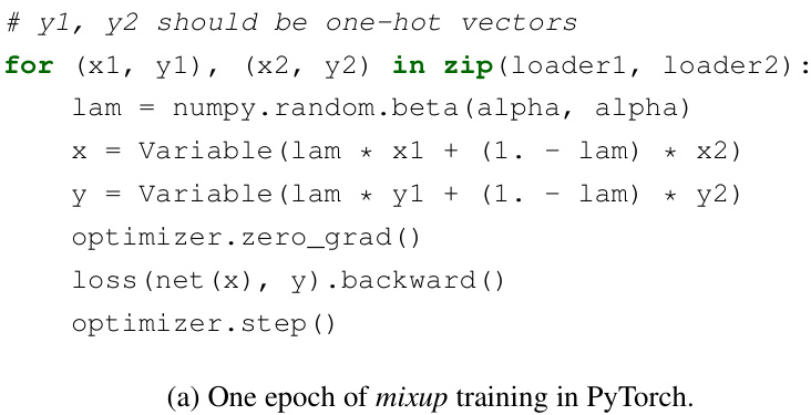
Figure 1: Illustration of mixup, which converges to ERM as $\alpha\rightarrow0$ .
图 1: mixup方法示意图,当$\alpha\rightarrow0$时收敛于ERM。
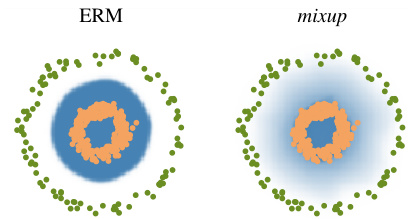
(b) Effect of mixup $\textit{\xi}\alpha=1$ ) on a toy problem. Green: Class 0. Orange: Class 1. Blue shading indicates $p(\boldsymbol{j}=1|\boldsymbol{x})$ .
(b) 混合增强 (mixup) ( $\textit{\xi}\alpha=1$ ) 在玩具问题上的效果。绿色: 类别0。橙色: 类别1。蓝色阴影表示 $p(\boldsymbol{j}=1|\boldsymbol{x})$ 。
However, the naive estimate $P_{\delta}$ is one out of many possible choices to approximate the true distribution $P$ . For instance, in the Vicinal Risk Minimization (VRM) principle (Chapelle et al., 2000), the distribution $P$ is approximated by
然而,朴素的估计 $P_{\delta}$ 只是众多可能用于近似真实分布 $P$ 的选择之一。例如,在邻域风险最小化 (Vicinal Risk Minimization, VRM) 原则中 (Chapelle et al., 2000),分布 $P$ 通过...
$$
P_{\nu}(\tilde{x},\tilde{y})=\frac{1}{n}\sum_{i=1}^{n}\nu(\tilde{x},\tilde{y}|x_{i},y_{i}),
$$
$$
P_{\nu}(\tilde{x},\tilde{y})=\frac{1}{n}\sum_{i=1}^{n}\nu(\tilde{x},\tilde{y}|x_{i},y_{i}),
$$
where $\nu$ is a vicinity distribution that measures the probability of finding the virtual feature-target pair $(\tilde{x},\tilde{y})$ in the vicinity of the training feature-target pair $(x_{i},y_{i})$ . In particular, Chapelle et al. (2000) considered Gaussian vicinities $\nu(\tilde{x},\tilde{y}|x_{i},y_{i})=\mathcal{N}(\tilde{x}-x_{i},\sigma^{2})\delta(\tilde{y}=y_{i})$ , which is equivalent to augmenting the training data with additive Gaussian noise. To learn using VRM, we sample the vicinal distribution to construct a dataset $\mathcal{D}_ {\nu}:={(\tilde{x}_ {i},\tilde{y}_ {i})}_{i=1}^{m}$ , and minimize the empirical vicinal risk:
其中 $\nu$ 是衡量在训练特征-目标对 $(x_{i},y_{i})$ 附近找到虚拟特征-目标对 $(\tilde{x},\tilde{y})$ 概率的邻域分布。特别地,Chapelle et al. (2000) 考虑了高斯邻域 $\nu(\tilde{x},\tilde{y}|x_{i},y_{i})=\mathcal{N}(\tilde{x}-x_{i},\sigma^{2})\delta(\tilde{y}=y_{i})$ ,这等同于通过添加高斯噪声来增强训练数据。为了使用VRM进行学习,我们从邻域分布中采样以构建数据集 $\mathcal{D}_ {\nu}:={(\tilde{x}_ {i},\tilde{y}_ {i})}_{i=1}^{m}$ ,并最小化经验邻域风险:
$$
R_{\nu}(f)=\frac{1}{m}\sum_{i=1}^{m}\ell(f(\tilde{x}_ {i}),\tilde{y}_{i}).
$$
$$
R_{\nu}(f)=\frac{1}{m}\sum_{i=1}^{m}\ell(f(\tilde{x}_ {i}),\tilde{y}_{i}).
$$
The contribution of this paper is to propose a generic vicinal distribution, called mixup:
本文的贡献是提出了一种通用的邻近分布方法,称为mixup:
$$
\mu(\tilde{x},\tilde{y}|x_{i},y_{i})=\frac{1}{n}\sum_{j}^{n}\mathbb{E}\left[\delta(\tilde{x}=\lambda\cdot x_{i}+(1-\lambda)\cdot x_{j},\tilde{y}=\lambda\cdot y_{i}+(1-\lambda)\cdot y_{j})\right],
$$
$$
\mu(\tilde{x},\tilde{y}|x_{i},y_{i})=\frac{1}{n}\sum_{j}^{n}\mathbb{E}\left[\delta(\tilde{x}=\lambda\cdot x_{i}+(1-\lambda)\cdot x_{j},\tilde{y}=\lambda\cdot y_{i}+(1-\lambda)\cdot y_{j})\right],
$$
where $\lambda\sim\operatorname{Beta}(\alpha,\alpha)$ , for $\alpha\in(0,\infty)$ . In a nutshell, sampling from the mixup vicinal distribution produces virtual feature-target vectors
其中 $\lambda\sim\operatorname{Beta}(\alpha,\alpha)$,$\alpha\in(0,\infty)$。简而言之,从 mixup 邻域分布中采样可生成虚拟特征-目标向量
$$
\begin{array}{r}{\tilde{x}=\lambda x_{i}+(1-\lambda)x_{j},}\ {\tilde{y}=\lambda y_{i}+(1-\lambda)y_{j},}\end{array}
$$
$$
\begin{array}{r}{\tilde{x}=\lambda x_{i}+(1-\lambda)x_{j},}\ {\tilde{y}=\lambda y_{i}+(1-\lambda)y_{j},}\end{array}
$$
where $(x_{i},y_{i})$ and $(x_{j},y_{j})$ are two feature-target vectors drawn at random from the training data, and $\lambda\in[0,1]$ . The mixup hyper-parameter $\alpha$ controls the strength of interpolation between feature-target pairs, recovering the ERM principle as $\alpha\rightarrow0$ .
其中 $(x_{i},y_{i})$ 和 $(x_{j},y_{j})$ 是从训练数据中随机抽取的两个特征-目标向量,且 $\lambda\in[0,1]$。混合超参数 $\alpha$ 控制特征-目标对之间的插值强度,当 $\alpha\rightarrow0$ 时恢复为经验风险最小化 (ERM) 原则。
The implementation of mixup training is straightforward, and introduces a minimal computation overhead. Figure 1a shows the few lines of code necessary to implement mixup training in PyTorch. Finally, we mention alternative design choices. First, in preliminary experiments we find that convex combinations of three or more examples with weights sampled from a Dirichlet distribution does not provide further gain, but increases the computation cost of mixup. Second, our current implementation uses a single data loader to obtain one minibatch, and then mixup is applied to the same minibatch after random shuffling. We found this strategy works equally well, while reducing I/O requirements. Third, interpolating only between inputs with equal label did not lead to the performance gains of mixup discussed in the sequel. More empirical comparison can be found in Section 3.8.
mixup训练的实现非常简单,且仅引入极小的计算开销。图1a展示了在PyTorch中实现mixup训练所需的几行代码。最后,我们讨论其他设计方案。首先,在初步实验中,我们发现从狄利克雷分布(Dirichlet distribution)采样权重对三个或更多样本进行凸组合并未带来额外收益,反而增加了mixup的计算成本。其次,当前实现使用单一数据加载器获取一个小批量(minibatch),随后对该批次随机打乱后应用mixup。该策略在保持同等效果的同时降低了I/O需求。第三,仅在相同标签的输入之间进行插值无法获得后文讨论的mixup性能优势。更多实验对比见第3.8节。
What is mixup doing? The mixup vicinal distribution can be understood as a form of data augmentation that encourages the model $f$ to behave linearly in-between training examples. We argue that this linear behaviour reduces the amount of undesirable oscillations when predicting outside the training examples. Also, linearity is a good inductive bias from the perspective of Occam’s razor,
mixup在做什么?mixup邻近分布可以理解为一种数据增强形式,它鼓励模型$f$在训练样本之间表现出线性行为。我们认为这种线性行为能减少在训练样本之外进行预测时的不良振荡。此外,从奥卡姆剃刀原则的角度来看,线性性是一种良好的归纳偏差。
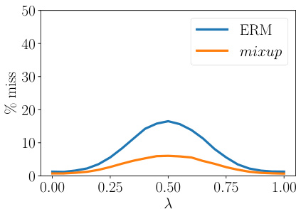
(a) Prediction errors in-between training data. Evaluated at $x=\lambda x_{i}+(1-\lambda)x_{j}$ , a prediction is counted as a “miss” if it does not belong to ${y_{i},y_{j}}$ . The model trained with mixup has fewer misses.
(a) 训练数据间的预测误差。在$x=\lambda x_{i}+(1-\lambda)x_{j}$处评估时,若预测值不属于${y_{i},y_{j}}$则记为"失误"。采用mixup训练的模型失误更少。
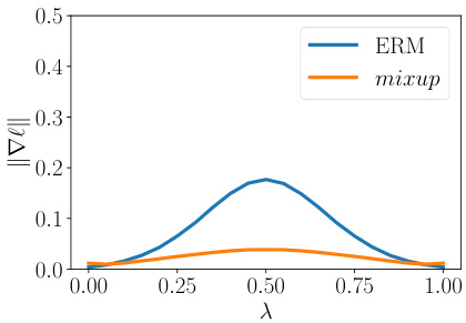
(b) Norm of the gradients of the model w.r.t. input in-between training data, evaluated at $x=\lambda x_{i}+$ $(1-\lambda)x_{j}$ . The model trained with mixup has smaller gradient norms.
图 1:
(b) 模型在训练数据间输入梯度范数,评估点为 $x=\lambda x_{i}+$ $(1-\lambda)x_{j}$。使用 mixup 训练的模型具有更小的梯度范数。
Figure 2: mixup leads to more robust model behaviors in-between the training data. Table 1: Validation errors for ERM and mixup on the development set of ImageNet-2012.
| Model | Method | Epochs | Top-1 Error | Top-5 Error |
| ResNet-50 | ERM (Goyal et al., 2017) | 90 | 23.5 | |
| mixup α = 0.2 | 90 | 23.3 | 6.6 | |
| ResNet-101 | ERM (Goyal et al., 2017) | 90 | 22.1 | |
| mixup α = 0.2 | 90 | 21.5 | 5.6 | |
| ResNeXt-101 32*4d | ERM (Xie et al., 2016) | 100 | 21.2 | |
| ERM | 90 | 21.2 | 5.6 | |
| mixup α = 0.4 | 90 | 20.7 | 5.3 | |
| ResNeXt-101 64*4d | ERM (Xie et al., 2016) | 100 | 20.4 | 5.3 |
| mixupα =0.4 | 90 | 19.8 | 4.9 | |
| ResNet-50 | ERM | 200 | 23.6 | 7.0 |
| mixup α = 0.2 | 200 | 22.1 | 6.1 | |
| ResNet-101 | ERM | 200 | 22.0 | 6.1 |
| mixup α = 0.2 | 200 | 20.8 | 5.4 | |
| ResNeXt-101 32*4d | ERM | 200 | 21.3 | 5.9 |
| mixup α = 0.4 | 200 | 20.1 | 5.0 |
图 2: mixup 使模型在训练数据之间表现出更鲁棒的行为。
表 1: ImageNet-2012 开发集上 ERM 和 mixup 的验证错误率。
| 模型 | 方法 | 训练轮数 | Top-1 错误率 | Top-5 错误率 |
|---|---|---|---|---|
| ResNet-50 | ERM (Goyal et al., 2017) | 90 | 23.5 | - |
| mixup α = 0.2 | 90 | 23.3 | 6.6 | |
| ResNet-101 | ERM (Goyal et al., 2017) | 90 | 22.1 | - |
| mixup α = 0.2 | 90 | 21.5 | 5.6 | |
| ResNeXt-101 32*4d | ERM (Xie et al., 2016) | 100 | 21.2 | - |
| ERM | 90 | 21.2 | 5.6 | |
| mixup α = 0.4 | 90 | 20.7 | 5.3 | |
| ResNeXt-101 64*4d | ERM (Xie et al., 2016) | 100 | 20.4 | 5.3 |
| mixup α = 0.4 | 90 | 19.8 | 4.9 | |
| ResNet-50 | ERM | 200 | 23.6 | 7.0 |
| mixup α = 0.2 | 200 | 22.1 | 6.1 | |
| ResNet-101 | ERM | 200 | 22.0 | 6.1 |
| mixup α = 0.2 | 200 | 20.8 | 5.4 | |
| ResNeXt-101 32*4d | ERM | 200 | 21.3 | 5.9 |
| mixup α = 0.4 | 200 | 20.1 | 5.0 |
since it is one of the simplest possible behaviors. Figure 1b shows that mixup leads to decision boundaries that transition linearly from class to class, providing a smoother estimate of uncertainty. Figure 2 illustrate the average behaviors of two neural network models trained on the CIFAR-10 dataset using ERM and mixup. Both models have the same architecture, are trained with the same procedure, and are evaluated at the same points in-between randomly sampled training data. The model trained with mixup is more stable in terms of model predictions and gradient norms in-between training samples.
因为它是最简单的行为之一。图1b显示,mixup会导致决策边界在类别之间线性过渡,从而提供更平滑的不确定性估计。图2展示了在CIFAR-10数据集上使用ERM和mixup训练的两种神经网络模型的平均行为。两个模型具有相同的架构,采用相同的训练流程,并在随机采样的训练数据之间的相同点进行评估。使用mixup训练的模型在训练样本之间的模型预测和梯度范数方面更加稳定。
3 EXPERIMENTS
3 实验
3.1 IMAGENET CLASSIFICATION
3.1 IMAGENET 分类
We evaluate mixup on the ImageNet-2012 classification dataset (Russ a kov sky et al., 2015). This dataset contains 1.3 million training images and 50,000 validation images, from a total of 1,000 classes. For training, we follow standard data augmentation practices: scale and aspect ratio distortions, random crops, and horizontal flips (Goyal et al., 2017). During evaluation, only the $224\times224$ central crop of each image is tested. We use mixup and ERM to train several state-of-the-art ImageNet-2012 classification models, and report both top-1 and top-5 error rates in Table 1.
我们在ImageNet-2012分类数据集(Russakovsky et al., 2015)上评估mixup方法。该数据集包含130万张训练图像和5万张验证图像,共1000个类别。训练阶段采用标准数据增强方法:尺度与长宽比畸变、随机裁剪和水平翻转(Goyal et al., 2017)。评估时仅测试每张图像$224\times224$的中心裁剪区域。我们使用mixup和ERM训练了多个先进的ImageNet-2012分类模型,并在表1中报告了top-1和top-5错误率。
Figure 3: Test errors for ERM and mixup on the CIFAR experiments.
| Dataset | Model | ERM | mixup |
| CIFAR-10 | PreActResNet-18 | 5.6 | 4.2 |
| WideResNet-28-10 DenseNet-BC-190 | 3.8 3.7 | 2.7 2.7 | |
| CIFAR-100 | PreActResNet-18 | 25.6 | 21.1 |
| WideResNet-28-10 | 19.4 | 17.5 | |
| DenseNet-BC-190 | 19.0 | 16.8 | |
(a) Test errors for the CIFAR experiments.
图 3: CIFAR实验中ERM和mixup的测试误差。
| 数据集 | 模型 | ERM | mixup |
|---|---|---|---|
| CIFAR-10 | PreActResNet-18 | 5.6 | 4.2 |
| CIFAR-10 | WideResNet-28-10 DenseNet-BC-190 | 3.8 3.7 | 2.7 2.7 |
| CIFAR-100 | PreActResNet-18 | 25.6 | 21.1 |
| CIFAR-100 | WideResNet-28-10 | 19.4 | 17.5 |
| DenseNet-BC-190 | 19.0 | 16.8 |
(a) CIFAR实验的测试误差。
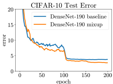
(b) Test error evolution for the best ERM and mixup models.
图 1:
(b) 最佳经验风险最小化 (ERM) 和 mixup 模型的测试误差变化曲线
For all the experiments in this section, we use data-parallel distributed training in Caffe21 with a minibatch size of 1,024. We use the learning rate schedule described in (Goyal et al., 2017). Specifically, the learning rate is increased linearly from 0.1 to 0.4 during the first 5 epochs, and it is then divided by 10 after 30, 60 and 80 epochs when training for 90 epochs; or after 60, 120 and 180 epochs when training for 200 epochs.
在本节所有实验中,我们使用Caffe21框架进行数据并行分布式训练,最小批次(batch)大小为1,024。学习率调度采用(Goyal et al., 2017)所述方案:前5个周期(epoch)从0.1线性增至0.4,随后在90周期训练时分别于30/60/80周期后除以10;200周期训练时则于60/120/180周期后进行相同衰减。
For mixup, we find that $\alpha\in[0.1,0.4]$ leads to improved performance over ERM, whereas for large $\alpha$ , mixup leads to under fitting. We also find that models with higher capacities and/or longer training runs are the ones to benefit the most from mixup. For example, when trained for 90 epochs, the mixup variants of ResNet-101 and ResNeXt-101 obtain a greater improvement ( $0.5%$ to $0.6%$ ) over their ERM analogues than the gain of smaller models such as ResNet-50 $(0.2%)$ . When trained for 200 epochs, the top-1 error of the mixup variant of ResNet-50 is further reduced by $1.2%$ compared to the 90 epoch run, whereas its ERM analogue stays the same.
对于mixup,我们发现当$\alpha\in[0.1,0.4]$时,其性能优于ERM(经验风险最小化),而当$\alpha$较大时,mixup会导致欠拟合。我们还发现,具有更高容量和/或更长训练周期的模型从mixup中获益最大。例如,在训练90个周期时,ResNet-101和ResNeXt-101的mixup变体相比其ERM对应模型获得了更大的提升($0.5%$至$0.6%$),而较小模型如ResNet-50的提升较小($0.2%$)。当训练周期延长至200个周期时,ResNet-50的mixup变体的top-1错误率相比90个周期的训练进一步降低了$1.2%$,而其ERM对应模型的性能保持不变。
3.2 CIFAR-10 AND CIFAR-100
3.2 CIFAR-10 与 CIFAR-100
We conduct additional image classification experiments on the CIFAR-10 and CIFAR-100 datasets to further evaluate the generalization performance of mixup. In particular, we compare ERM and mixup training for: PreAct ResNet-18 (He et al., 2016) as implemented in (Liu, 2017), WideResNet28-10 (Zagoruyko & Komodakis, 2016a) as implemented in (Zagoruyko & Komodakis, 2016b), and DenseNet (Huang et al., 2017) as implemented in (Veit, 2017). For DenseNet, we change the growth rate to 40 to follow the DenseNet-BC-190 specification from (Huang et al., 2017). For mixup, we fix $\alpha=1$ , which results in interpolations $\lambda$ uniformly distributed between zero and one. All models are trained on a single Nvidia Tesla P100 GPU using PyTorch2 for 200 epochs on the training set with 128 examples per minibatch, and evaluated on the test set. Learning rates start at 0.1 and are divided by 10 after 100 and 150 epochs for all models except WideResNet. For WideResNet, we follow (Zagoruyko & Komodakis, 2016a) and divide the learning rate by 10 after 60, 120 and 180 epochs. Weight decay is set to $10^{-4}$ . We do not use dropout in these experiments.
我们在CIFAR-10和CIFAR-100数据集上进行了额外的图像分类实验,以进一步评估mixup的泛化性能。具体而言,我们比较了以下模型的ERM和mixup训练:采用(Liu, 2017)实现的PreAct ResNet-18 (He et al., 2016)、采用(Zagoruyko & Komodakis, 2016b)实现的WideResNet28-10 (Zagoruyko & Komodakis, 2016a),以及采用(Veit, 2017)实现的DenseNet (Huang et al., 2017)。对于DenseNet,我们将增长率调整为40以符合(Huang et al., 2017)中的DenseNet-BC-190规格。mixup实验中固定超参数$\alpha=1$,这使得插值系数$\lambda$在0到1之间均匀分布。所有模型均在Nvidia Tesla P100 GPU上使用PyTorch2进行训练,每个小批量包含128个样本,共训练200个epoch,并在测试集上评估性能。除WideResNet外,所有模型的初始学习率为0.1,并在第100和150个epoch后降至十分之一。对于WideResNet,我们遵循(Zagoruyko & Komodakis, 2016a)的设置,在第60、120和180个epoch后将学习率降至十分之一。权重衰减设置为$10^{-4}$,本实验未使用dropout。
We summarize our results in Figure 3a. In both CIFAR-10 and CIFAR-100 classification problems, the models trained using mixup significantly outperform their analogues trained with ERM. As seen in Figure 3b, mixup and ERM converge at a similar speed to their best test errors. Note that the DenseNet models in (Huang et al., 2017) were trained for 300 epochs with further learning rate decays scheduled at the 150 and 225 epochs, which may explain the discrepancy the performance of DenseNet reported in Figure 3a and the original result of Huang et al. (2017).
我们在图 3a 中总结了实验结果。在 CIFAR-10 和 CIFAR-100 分类任务中,使用 mixup 训练的模型显著优于采用经验风险最小化 (ERM) 训练的对应模型。如图 3b 所示,mixup 和 ERM 以相近的速度收敛至最佳测试误差。需要注意的是,(Huang et al., 2017) 中的 DenseNet 模型训练了 300 个周期,并在第 150 和 225 个周期安排了额外的学习率衰减,这可能是图 3a 报告的 DenseNet 性能与 Huang et al. (2017) 原始结果存在差异的原因。
3.3 SPEECH DATA
3.3 语音数据
Next, we perform speech recognition experiments using the Google commands dataset (Warden, 2017). The dataset contains 65,000 utterances, where each utterance is about one-second long and belongs to one out of 30 classes. The classes correspond to voice commands such as yes, no, down, left, as pronounced by a few thousand different speakers. To preprocess the utterances, we first extract normalized spec tro grams from the original waveforms at a sampling rate of $16\mathrm{kHz}$ . Next, we zero-pad the spec tro grams to equalize their sizes at $160\times101$ . For speech data, it is reasonable to apply mixup both at the waveform and spec tr ogram levels. Here, we apply mixup at the spec tr ogram level just before feeding the data to the network.
接下来,我们使用Google语音命令数据集(Warden, 2017)进行语音识别实验。该数据集包含65,000条语音片段,每条时长约1秒,属于30个类别之一。这些类别对应着数千名不同发音人所说的yes、no、down、left等语音指令。
在预处理阶段,我们首先从原始波形中以$16\mathrm{kHz}$的采样率提取归一化的频谱图(spec tro gram)。接着,我们将频谱图零填充至统一尺寸$160\times101$。对于语音数据,在波形和频谱图两个层面应用混合增强(mixup)都是合理的。本实验中,我们在将数据输入网络前,仅在频谱图层面应用了混合增强。
Figure 4: Classification errors of ERM and mixup on the Google commands dataset.
| Model | Method | Validationset | Testset |
| LeNet | ERM | 9.8 | 10.3 |
| mixup (α =0.1) | 10.1 | 10.8 | |
| mixup (Q = 0.2) | 10.2 | 11.3 | |
| VGG-11 | ERM | 5.0 | 4.6 |
| mixup (α = 0.1) | 4.0 | 3.8 | |
| mixup (α =0.2) | 3.9 | 3.4 |
图 4: Google commands数据集中ERM和mixup的分类错误
| 模型 | 方法 | 验证集 | 测试集 |
|---|---|---|---|
| LeNet | ERM | 9.8 | 10.3 |
| mixup (α=0.1) | 10.1 | 10.8 | |
| mixup (α=0.2) | 10.2 | 11.3 | |
| VGG-11 | ERM | 5.0 | 4.6 |
| mixup (α=0.1) | 4.0 | 3.8 | |
| mixup (α=0.2) | 3.9 | 3.4 |
For this experiment, we compare a LeNet (Lecun et al., 2001) and a VGG-11 (Simonyan & Zisserman, 2015) architecture, each of them composed by two convolutional and two fully-connected layers. We train each model for 30 epochs with mini batches of 100 examples, using Adam as the optimizer (Kingma & Ba, 2015). Training starts with a learning rate equal to $3\times10^{-3}$ and is divided by 10 every 10 epochs. For mixup, we use a warm-up period of five epochs where we train the network on original training examples, since we find it speeds up initial convergence. Table 4 shows that mixup outperforms ERM on this task, specially when using VGG-11, the model with larger capacity.
在本实验中,我们比较了LeNet (Lecun et al., 2001) 和VGG-11 (Simonyan & Zisserman, 2015) 架构,每个架构由两个卷积层和两个全连接层组成。我们使用Adam优化器 (Kingma & Ba, 2015),以100个样本为小批量,对每个模型进行30轮训练。初始学习率为 $3\times10^{-3}$,每10轮学习率除以10。对于mixup方法,我们设置了5轮的预热期,在此期间使用原始训练样本训练网络,因为我们发现这能加速初始收敛。表4显示,mixup在该任务上优于ERM(经验风险最小化),尤其是在使用容量更大的VGG-11模型时。
3.4 MEMORIZATION OF CORRUPTED LABELS
3.4 损坏标签的记忆
Following Zhang et al. (2017), we evaluate the robustness of ERM and mixup models against randomly corrupted labels. We hypothesize that increasing the strength of mixup interpolation $\alpha$ should generate virtual examples further from the training examples, making memorization more difficult to achieve. In particular, it should be easier to learn interpolations between real examples compared to memorizing interpolations involving random labels. We adapt an open-source implementation (Zhang, 2017) to generate three CIFAR-10 training sets, where $20%$ , $50%$ , or $80%$ of the labels are replaced by random noise, respectively. All the test labels are kept intact for evaluation. Dropout (Srivastava et al., 2014) is considered the state-of-the-art method for learning with corrupted labels (Arpit et al., 2017). Thus, we compare in these experiments mixup, dropout, mixup $^+$ dropout, and ERM. For mixup, we choose $\alpha\in{1,2,8,32}$ ; for dropout, we add one dropout layer in each PreAct block after the ReLU activation layer between two convolution layers, as suggested in (Zagoruyko & Komodakis, 2016a). We choose the dropout probability $p\in{0.5,0.7,0.8,\overset{\cdot}{0.}9}$ . For the combination of mixup and dropout, we choose $\alpha\in{1,2,4,8}$ and $p\in{0.3,0.5,0.7}$ . These experiments use the PreAct ResNet-18 (He et al., 2016) model implemented in (Liu, 2017). All the other settings are the same as in Section 3.2.
遵循Zhang等人(2017)的方法,我们评估了ERM和mixup模型对随机损坏标签的鲁棒性。我们假设增加mixup插值强度$\alpha$会生成远离训练样本的虚拟样本,使记忆更难实现。特别是与记忆涉及随机标签的插值相比,学习真实样本之间的插值应该更容易。我们采用开源实现(Zhang, 2017)生成三个CIFAR-10训练集,分别将$20%$、$50%$或$80%$的标签替换为随机噪声。所有测试标签保持完整用于评估。Dropout (Srivastava等人, 2014)被认为是学习损坏标签的最先进方法(Arpit等人, 2017)。因此,我们在这些实验中比较了mixup、dropout、mixup$^+$dropout和ERM。对于mixup,我们选择$\alpha\in{1,2,8,32}$;对于dropout,如(Zagoruyko & Komodakis, 2016a)建议,我们在两个卷积层之间的ReLU激活层后,在每个PreAct块中添加一个dropout层。我们选择dropout概率$p\in{0.5,0.7,0.8,\overset{\cdot}{0.}9}$。对于mixup和dropout的组合,我们选择$\alpha\in{1,2,4,8}$和$p\in{0.3,0.5,0.7}$。这些实验使用(Liu, 2017)中实现的PreAct ResNet-18 (He等人, 2016)模型。所有其他设置与第3.2节相同。
We summarize our results in Table 2, where we note the best test error achieved during the training session, as well as the final test error after 200 epochs. To quantify the amount of memorization, we also evaluate the training errors at the last epoch on real labels and corrupted labels. As the training progresses with a smaller learning rate (e.g. less than 0.01), the ERM model starts to overfit the corrupted labels. When using a large probability (e.g. 0.7 or 0.8), dropout can effectively reduce over fitting. mixup with a large $\alpha$ (e.g. 8 or 32) outperforms dropout on both the best and last epoch test errors, and achieves lower training error on real labels while remaining resistant to noisy labels. Interestingly, mixup $^+$ dropout performs the best of all, showing that the two methods are compatible.
我们在表2中总结了实验结果,记录了训练过程中达到的最佳测试误差以及200个周期后的最终测试误差。为量化记忆程度,我们还评估了最后一个周期在真实标签和损坏标签上的训练误差。当采用较小学习率(如低于0.01)进行训练时,ERM模型开始对损坏标签过拟合。使用较高概率(如0.7或0.8)时,dropout能有效减轻过拟合现象。采用较大$\alpha$值(如8或32)的mixup在最佳测试误差和最终测试误差上都优于dropout,在保持对噪声标签鲁棒性的同时,对真实标签实现了更低的训练误差。值得注意的是,mixup$^+$dropout的组合取得了最佳效果,表明这两种方法具有兼容性。
3.5 ROBUSTNESS TO ADVERSARIAL EXAMPLES
3.5 对抗样本的鲁棒性
One undesirable consequence of models trained using ERM is their fragility to adversarial examples (Szegedy et al., 2014). Adversarial examples are obtained by adding tiny (visually imperceptible) perturbations to legitimate examples in order to deteriorate the performance of the model. The adversarial noise is generated by ascending the gradient of the loss surface with respect to the legitimate example. Improving the robustness to adversarial examples is a topic of active research.
使用经验风险最小化(ERM)训练的模型会产生一个不良后果:它们对对抗样本(Szegedy et al., 2014)的脆弱性。对抗样本是通过对合法样本添加微小(视觉上难以察觉)的扰动来获得的,目的是降低模型的性能。这种对抗噪声是通过沿着合法样本的损失梯度上升方向生成的。提高对抗样本的鲁棒性是一个活跃的研究课题。
Table 2: Results on the corrupted label experiments for the best models.
| Label corruption | Method | Test error | Training error | ||
| Best | Last | Real | Corrupted | ||
| 20% | ERM | 12.7 | 16.6 | 0.05 | 0.28 |
| ERM + dropout (p = 0.7) | 8.8 | 10.4 | 5.26 | 83.55 | |
| mixup(α=8) | 5.9 | 6.4 | 2.27 | 86.32 | |
| mixup + dropout (α = 4,p = 0.1) | 6.2 | 6.2 | 1.92 | 85.02 | |
| 50% | ERM | 18.8 | 44.6 | 0.26 | 0.64 |
| ERM + dropout (p = 0.8) | 14.1 | 15.5 | 12.71 | 86.98 | |
| mixup(α =32) | 11.3 | 12.7 | 5.84 | 85.71 | |
| mixup + dropout (α = 8,p = 0.3) | 10.9 | 10.9 | 7.56 | 87.90 | |
| 80% | ERM | 36.5 | 73.9 | 0.62 | 0.83 |
| ERM + dropout (p = 0.8) | 30.9 | 35.1 | 29.84 | 86.37 | |
| mixup (α =32) | 25.3 | 30.9 | 18.92 | 85.44 | |
| mixup + dropout (α = 8,p = 0.3) | 24.0 | 24.8 | 19.70 | 87.67 | |
表 2: 最佳模型在标签损坏实验中的结果
| 标签损坏 | 方法 | 测试误差 | 训练误差 | ||
|---|---|---|---|---|---|
| 最佳 | 最后 | 真实 | 损坏 | ||
| 20% | ERM | 12.7 | 16.6 | 0.05 | 0.28 |
| ERM + dropout (p = 0.7) | 8.8 | 10.4 | 5.26 | 83.55 | |
| mixup(α=8) | 5.9 | 6.4 | 2.27 | 86.32 | |
| mixup + dropout (α = 4,p = 0.1) | 6.2 | 6.2 | 1.92 | 85.02 | |
| 50% | ERM | 18.8 | 44.6 | 0.26 | 0.64 |
| ERM + dropout (p = 0.8) | 14.1 | 15.5 | 12.71 | 86.98 | |
| mixup(α =32) | 11.3 | 12.7 | 5.84 | 85.71 | |
| mixup + dropout (α = 8,p = 0.3) | 10.9 | 10.9 | 7.56 | 87.90 | |
| 80% | ERM | 36.5 | 73.9 | 0.62 | 0.83 |
| ERM + dropout (p = 0.8) | 30.9 | 35.1 | 29.84 | 86.37 | |
| mixup (α =32) | 25.3 | 30.9 | 18.92 | 85.44 | |
| mixup + dropout (α = 8,p = 0.3) | 24.0 | 24.8 | 19.70 | 87.67 |
| Metric | Method | FGSM | I-FGSM |
| Top-1 | ERM | 57.0 | 57.3 |
| mixup | 46.0 | 40.9 | |
| Top-5 | ERM | 24.8 | 18.1 |
| mixup | 17.4 | 11.8 |
| 指标 | 方法 | FGSM | I-FGSM |
|---|---|---|---|
| Top-1 | ERM | 57.0 | 57.3 |
| mixup | 46.0 | 40.9 | |
| Top-5 | ERM | 24.8 | 18.1 |
| mixup | 17.4 | 11.8 |
Table 3: Classification errors of ERM and mixup models when tested on adversarial examples.
| Metric | Method | FGSM | I-FGSM |
| Top-1 | ERM | 90.7 | 99.9 |
| mixup | 75.2 | 99.6 | |
| Top-5 | ERM | 63.1 | 93.4 |
| mixup | 49.1 | 95.8 |
(a) White box attacks. (b) Black box attacks.
表 3: ERM 和 mixup 模型在对抗样本测试中的分类错误
| 指标 | 方法 | FGSM | I-FGSM |
|---|---|---|---|
| Top-1 | ERM | 90.7 | 99.9 |
| mixup | 75.2 | 99.6 | |
| Top-5 | ERM | 63.1 | 93.4 |
| mixup | 49.1 | 95.8 |
(a) 白盒攻击。 (b) 黑盒攻击。
Among the several methods aiming to solve this problem, some have proposed to penalize the norm of the Jacobian of the model to control its Lipschitz constant (Drucker & Le Cun, 1992; Cisse et al., 2017; Bartlett et al., 2017; Hein & And ri ush chen ko, 2017). Other approaches perform data augmentation by producing and training on adversarial examples (Goodfellow et al., 2015). Unfortunately, all of these methods add significant computational overhead to ERM. Here, we show that mixup can significantly improve the robustness of neural networks without hindering the speed of ERM by penalizing the norm of the gradient of the loss w.r.t a given input along the most plausible directions (e.g. the directions to other training points). Indeed, Figure 2 shows that mixup results in models having a smaller loss and gradient norm between examples compared to vanilla ERM.
在解决该问题的多种方法中,部分研究提出通过惩罚模型雅可比矩阵(Jacobian)的范数来控制其利普希茨常数(Lipschitz constant) (Drucker & Le Cun, 1992; Cisse et al., 2017; Bartlett et al., 2017; Hein & Andriushchenko, 2017)。另一些方法则通过生成对抗样本并进行训练来实现数据增强(Goodfellow et al., 2015)。遗憾的是,这些方法都会给经验风险最小化(ERM)带来显著的计算开销。本文证明,mixup能通过沿最合理方向(如指向其他训练样本的方向)惩罚损失函数对给定输入的梯度范数,在不影响ERM速度的前提下显著提升神经网络的鲁棒性。图2显示,与原始ERM相比,mixup能使模型在样本间获得更小的损失值和梯度范数。
To assess the robustness of mixup models to adversarial examples, we use three ResNet-101 models: two of them trained using ERM on ImageNet-2012, and the third trained using mixup. In the first set of experiments, we study the robustness of one ERM model and the mixup model against white box attacks. That is, for each of the two models, we use the model itself to generate adversarial examples, either using the Fast Gradient Sign Method (FGSM) or the Iterative FGSM (I-FGSM) methods (Goodfellow et al., 2015), allowing a maximum perturbation of $\epsilon=4$ for every pixel. For I-FGSM, we use 10 iterations with equal step size. In the second set of experiments, we evaluate robustness against black box attacks. That is, we use the first ERM model to produce adversarial examples using FGSM and I-FGSM. Then, we test the robustness of the second ERM model and the mixup model to these examples. The results of both settings are summarized in Table 3.
为了评估混合模型(mixup)对对抗样本的鲁棒性,我们使用了三个ResNet-101模型:其中两个通过ERM在ImageNet-2012上训练,第三个使用mixup方法训练。在第一组实验中,我们研究了一个ERM模型和mixup模型对白盒攻击的鲁棒性。具体而言,对于这两个模型中的每一个,我们使用模型本身生成对抗样本,采用快速梯度符号法(FGSM)或迭代FGSM(I-FGSM)方法[20],允许每个像素的最大扰动为$\epsilon=4$。对于I-FGSM,我们使用10次等步长迭代。在第二组实验中,我们评估了模型对黑盒攻击的鲁棒性。即使用第一个ERM模型通过FGSM和I-FGSM生成对抗样本,然后测试第二个ERM模型和mixup模型对这些样本的鲁棒性。两种设置的结果总结在表3中。
For the FGSM white box attack, the mixup model is 2.7 times more robust than the ERM model in terms of Top-1 error. For the FGSM black box attack, the mixup model is 1.25 times more robust than the ERM model in terms of Top-1 error. Also, while both mixup and ERM are not robust to white box I-FGSM attacks, mixup is about $40%$ more robust than ERM in the black box I-FGSM setting. Overall, mixup produces neural networks that are significantly more robust than ERM against adversarial examples in white box and black settings without additional overhead compared to ERM.
对于FGSM白盒攻击,mixup模型在Top-1错误率上的鲁棒性是ERM模型的2.7倍。对于FGSM黑盒攻击,mixup模型的Top-1错误率鲁棒性是ERM模型的1.25倍。此外,虽然mixup和ERM对白盒I-FGSM攻击都不具备鲁棒性,但在黑盒I-FGSM场景下,mixup的鲁棒性比ERM高出约$40%$。总体而言,与ERM相比,mixup生成的神经网络在白盒和黑盒场景下对对抗样本的鲁棒性显著提升,且无需额外开销。
| Dataset | ERM | mixup |
| Htru2 | 2.0 | 2.0 |
| Iris | 21.3 | 17.3 |
| Phishing | 16.3 | 15.2 |
| 数据集 | ERM | mixup |
|---|---|---|
| Htru2 | 2.0 | 2.0 |
| Iris | 21.3 | 17.3 |
| Phishing | 16.3 | 15.2 |
Table 4: ERM and mixup classification errors on the UCI datasets.
| Dataset | ERM | mixup |
| Abalone | 74.0 | 73.6 |
| Arcene | 57.6 | 48.0 |
| Arrhythmia | 56.6 | 46.3 |
表 4: UCI数据集上ERM和mixup的分类错误率。
| 数据集 | ERM | mixup |
|---|---|---|
| Abalone | 74.0 | 73.6 |
| Arcene | 57.6 | 48.0 |
| Arrhythmia | 56.6 | 46.3 |

Figure 5: Effect of mixup on stabilizing GAN training at iterations 10, 100, 1000, 10000, and 20000.
图 5: Mixup 在迭代次数为 10、100、1000、10000 和 20000 时对稳定 GAN 训练的效果。
3.6 TABULAR DATA
3.6 表格数据
To further explore the performance of mixup on non-image data, we performed a series of experiments on six arbitrary classification problems drawn from the UCI dataset (Lichman, 2013). The neural networks in this section are fully-connected, and have two hidden layers of 128 ReLU units. The parameters of these neural networks are learned using Adam (Kingma & Ba, 2015) with default hyper-parameters, over 10 epochs of mini-batches of size 16. Table 4 shows that mixup improves the average test error on four out of the six considered datasets, and never under performs ERM.
为了进一步探究mixup在非图像数据上的表现,我们在UCI数据集 (Lichman, 2013) 中选取了六个任意分类问题进行了系列实验。本节使用的神经网络均为全连接结构,包含两个具有128个ReLU单元的隐藏层。这些神经网络的参数采用Adam优化器 (Kingma & Ba, 2015) 进行训练,使用默认超参数,经过10轮次的小批量训练(批量大小为16)。表4显示,mixup在六个数据集中有四个的平均测试错误率得到改善,且从未表现逊于ERM方法。
3.7 STABILIZATION OF GENERATIVE ADVERSARIAL NETWORKS (GANS)
3.7 生成对抗网络 (GANs) 的稳定性
Generative Adversarial Networks, also known as GANs (Goodfellow et al., 2014), are a powerful family of implicit generative models. In GANs, a generator and a disc rim in at or compete against each other to model a distribution $P$ . On the one hand, the generator $g$ competes to transform noise vectors $z\sim Q$ into fake samples $g(z)$ that resemble real samples $x\sim P$ . On the other hand, the disc rim in at or competes to distinguish between real samples $x$ and fake samples $g(z)$ . Mathematically, training a GAN is equivalent to solving the optimization problem
生成对抗网络 (Generative Adversarial Networks, GANs) (Goodfellow et al., 2014) 是一类强大的隐式生成模型。在GAN中,生成器 (generator) 和判别器 (discriminator) 相互竞争以建模分布 $P$ 。一方面,生成器 $g$ 致力于将噪声向量 $z\sim Q$ 转换为与真实样本 $x\sim P$ 相似的伪造样本 $g(z)$ ;另一方面,判别器则试图区分真实样本 $x$ 和伪造样本 $g(z)$ 。从数学角度看,训练GAN等同于求解以下优化问题
$$
\operatorname*{max}_ {g}\operatorname*{min}_ {d}\mathbb{E}_{x,z}\ell(d(x),1)+\ell(d(g(z)),0),
$$
$$
\operatorname*{max}_ {g}\operatorname*{min}_ {d}\mathbb{E}_{x,z}\ell(d(x),1)+\ell(d(g(z)),0),
$$
where $\ell$ is the binary cross entropy loss. Unfortunately, solving the previous min-max equation is a notoriously difficult optimization problem (Goodfellow, 2016), since the disc rim in at or often provides the generator with vanishing gradients. We argue that mixup should stabilize GAN training because it acts as a regularize r on the gradients of the disc rim in at or, akin to the binary classifier in Figure 1b. Then, the smoothness of the disc rim in at or guarantees a stable source of gradient information to the generator. The mixup formulation of GANs is:
其中$\ell$是二元交叉熵损失。遗憾的是,求解上述极小极大方程是一个众所周知的困难优化问题 (Goodfellow, 2016),因为判别器(discriminator)常会为生成器提供消失的梯度。我们认为mixup应该能稳定GAN训练,因为它作为判别器梯度的正则化器(regularizer),类似于图1b中的二元分类器。此时,判别器的平滑性保证了生成器能获得稳定的梯度信息源。GAN的mixup公式为:
$$
\operatorname*{max}_ {g}\operatorname*{min}_{d}\underset{x,z,\lambda}{\mathbb{E}}\ell(d(\lambda x+(1-\lambda)g(z)),\lambda).
$$
$$
\operatorname*{max}_ {g}\operatorname*{min}_{d}\underset{x,z,\lambda}{\mathbb{E}}\ell(d(\lambda x+(1-\lambda)g(z)),\lambda).
$$
Figure 5 illustrates the stabilizing effect of mixup the training of GAN (orange samples) when modeling two toy datasets (blue samples). The neural networks in these experiments are fullyconnected and have three hidden layers of 512 ReLU units. The generator network accepts twodimensional Gaussian noise vectors. The networks are trained for 20,000 mini-batches of size 128 using the Adam optimizer with default parameters, where the disc rim in at or is trained for five iterations before every generator iteration. The training of mixup GANs seems promisingly robust to hyper-parameter and architectural choices.
图 5: 展示了在建模两个玩具数据集(蓝色样本)时,mixup对GAN训练(橙色样本)的稳定效果。这些实验中的神经网络均为全连接结构,包含三个具有512个ReLU单元的隐藏层。生成器网络接收二维高斯噪声向量作为输入。所有网络均使用默认参数的Adam优化器进行训练,共20,000个小批量(每批128个样本),其中判别器在每次生成器迭代前会进行五次训练。实验表明,mixup GANs的训练对于超参数和架构选择展现出良好的鲁棒性。
Table 5: Results of the ablation studies on the CIFAR-10 dataset. Reported are the median test errors of the last 10 epochs. A tick $(\checkmark)$ means the component is different from standard ERM training, whereas a cross $({\pmb X})$ means it follows the standard training practice. AC: mix between all classes. SC: mix within the same class. RP: mix between random pairs. KNN: mix between $\mathbf{k}$ -nearest neighbors $({\bf k}{=}200),$ ). Please refer to the text for details about the experiments and interpretations.
| Method | Specification | Modified | Weight decay | ||
| Input | Target | 10-4 | 5 × 10⁻⁴ | ||
| ERM | 5.53 | 5.18 | |||
| mixup | AC + RP | 4.24 | 4.68 | ||
| AC + KNN | 4.98 | 5.26 | |||
| mix labels and latent representations (AC + RP) | Layer 1 | √ | 4.44 | 4.51 | |
| Layer 2 | 4.56 | 4.61 | |||
| Layer 3 | 5.39 | 5.55 | |||
| Layer 4 | 5.95 | 5.43 | |||
| Layer 5 | 5.39 | 5.15 | |||
| mix inputs only | SC + KNN (Chawla et al., 2002) | × | 5.45 | 5.52 | |
| AC + KNN | × | 5.43 | 5.48 | ||
| SC + RP | 5.23 | 5.55 | |||
| AC + RP | × | 5.17 | 5.72 | ||
| label smoothing (Szegedy et al., 2016) | =0.05 | × | 5.25 | 5.02 | |
| =0.1 | × | 5.33 | 5.17 | ||
| =0.2 | × | 5.34 | 5.06 | ||
| mix inputs + label smoothing (AC + RP) | = 0.05 | 5.02 | 5.40 | ||
| =0.1 | 5.08 | 5.09 | |||
| =0.2 | 4.98 | 5.06 | |||
| =0.4 | 5.25 | 5.39 | |||
| add Gaussiannoise to inputs | 0 = 0.05 | × | 5.53 | 5.04 | |
| 0 =0.1 | × | 6.41 | 5.86 | ||
| 0 =0.2 | × | 7.16 | 7.24 | ||
表 5: CIFAR-10数据集消融研究结果。报告的是最后10个epoch的中值测试错误率。勾号 $(\checkmark)$ 表示该组件与标准ERM训练不同,而叉号 $({\pmb X})$ 表示遵循标准训练实践。AC: 所有类别间混合。SC: 同类别内混合。RP: 随机对间混合。KNN: $\mathbf{k}$-近邻间混合 $({\bf k}{=}200)$。实验细节和解释请参阅正文。
| 方法 | 规格 | 修改输入 | 修改目标 | 权重衰减 10-4 | 权重衰减 5 × 10⁻⁴ |
|---|---|---|---|---|---|
| ERM | 5.53 | 5.18 | |||
| mixup | AC + RP | 4.24 | 4.68 | ||
| mixup | AC + KNN | 4.98 | 5.26 | ||
| 混合标签和潜在表示 (AC + RP) | 第1层 | √ | 4.44 | 4.51 | |
| 混合标签和潜在表示 (AC + RP) | 第2层 | 4.56 | 4.61 | ||
| 混合标签和潜在表示 (AC + RP) | 第3层 | 5.39 | 5.55 | ||
| 混合标签和潜在表示 (AC + RP) | 第4层 | 5.95 | 5.43 | ||
| 混合标签和潜在表示 (AC + RP) | 第5层 | 5.39 | 5.15 | ||
| 仅混合输入 | SC + KNN (Chawla et al., 2002) | × | 5.45 | 5.52 | |
| 仅混合输入 | AC + KNN | × | 5.43 | 5.48 | |
| 仅混合输入 | SC + RP | 5.23 | 5.55 | ||
| 仅混合输入 | AC + RP | × | 5.17 | 5.72 | |
| 标签平滑 (Szegedy et al., 2016) | =0.05 | × | 5.25 | 5.02 | |
| 标签平滑 (Szegedy et al., 2016) | =0.1 | × | 5.33 | 5.17 | |
| 标签平滑 (Szegedy et al., 2016) | =0.2 | × | 5.34 | 5.06 | |
| 混合输入 + 标签平滑 (AC + RP) | =0.05 | 5.02 | 5.40 | ||
| 混合输入 + 标签平滑 (AC + RP) | =0.1 | 5.08 | 5.09 | ||
| 混合输入 + 标签平滑 (AC + RP) | =0.2 | 4.98 | 5.06 | ||
| 混合输入 + 标签平滑 (AC + RP) | =0.4 | 5.25 | 5.39 | ||
| 向输入添加高斯噪声 | 0=0.05 | × | 5.53 | 5.04 | |
| 向输入添加高斯噪声 | 0=0.1 | × | 6.41 | 5.86 | |
| 向输入添加高斯噪声 | 0=0.2 | × | 7.16 | 7.24 |
3.8 ABLATION STUDIES
3.8 消融实验
mixup is a data augmentation method that consists of only two parts: random convex combination of raw inputs, and correspondingly, convex combination of one-hot label encodings. However, there are several design choices to make. For example, on how to augment the inputs, we could have chosen to interpolate the latent representations (i.e. feature maps) of a neural network, and we could have chosen to interpolate only between the nearest neighbors, or only between inputs of the same class. When the inputs to interpolate come from two different classes, we could have chosen to assign a single label to the synthetic input, for example using the label of the input that weights more in the convex combination. To compare mixup with these alternative possibilities, we run a set of ablation study experiments using the PreAct ResNet-18 architecture on the CIFAR-10 dataset.
mixup是一种数据增强方法,仅包含两部分:原始输入的随机凸组合,以及对应的独热标签编码的凸组合。然而,这其中存在多个设计选择。例如,在如何增强输入方面,我们可以选择对神经网络潜在表示(即特征图)进行插值,也可以选择仅在最近邻之间或仅在同一类别输入之间进行插值。当插值输入来自两个不同类别时,我们可以选择为合成输入分配单一标签,例如使用凸组合中权重较大的输入标签。为了比较mixup与这些替代方案,我们在CIFAR-10数据集上使用PreAct ResNet-18架构进行了一系列消融实验。
Specifically, for each of the data augmentation methods, we test two weight decay settings $(10^{-4}$ which works well for mixup, and $5\bar{\times}10^{-4}$ which works well for ERM). All the other settings and hyper parameters are the same as reported in Section 3.2.
具体而言,针对每种数据增强方法,我们测试了两种权重衰减设置 $(10^{-4}$ (适用于mixup)和 $5\bar{\times}10^{-4}$ (适用于ERM) 。其余所有设置和超参数均与第3.2节报告的一致。
To compare interpolating raw inputs with interpolating latent representations, we test on random convex combination of the learned representations before each residual block (denoted Layer 1-4) or before the uppermost “average pooling $+$ fully connected” layer (denoted Layer 5). To compare mixing random pairs of inputs (RP) with mixing nearest neighbors (KNN), we first compute the 200 nearest neighbors for each training sample, either from the same class (SC) or from all the classes (AC). Then during training, for each sample in a minibatch, we replace the sample with a synthetic sample by convex combination with a random draw from its nearest neighbors. To compare mixing all the classes (AC) with mixing within the same class (SC), we convex combine a minibatch with a random permutation of its sample index, where the permutation is done in a per-batch basis (AC) or a per-class basis (SC). To compare mixing inputs and labels with mixing inputs only, we either use a convex combination of the two one-hot encodings as the target, or select the one-hot encoding of the closer training sample as the target. For label smoothing, we follow Szegedy et al. (2016) and use $\frac{\epsilon}{10}$ as the target for incorrect classes, and $\textstyle1-{\frac{9\epsilon}{10}}$ as the target for the correct class.Adding Gaussian noise to inputs is used as another baseline. We report the median test errors of the last 10 epochs. Results are shown in Table 5.
为了比较原始输入插值与潜在表示插值的效果,我们在每个残差块前(标记为层1-4)或最顶层的"平均池化$+$全连接"层前(标记为层5)对学习到的表示进行随机凸组合测试。为比较随机输入对混合(RP)与最近邻混合(KNN),我们首先为每个训练样本计算200个最近邻,这些最近邻可以来自同一类别(SC)或所有类别(AC)。在训练过程中,对于小批次中的每个样本,我们通过与其最近邻的随机样本进行凸组合来生成合成样本以替代原样本。为比较跨类别混合(AC)与同类别混合(SC),我们将小批次样本与其索引的随机排列进行凸组合,其中排列按批次(AC)或按类别(SC)进行。为比较输入标签混合与仅输入混合,我们采用两种方式:将两个独热编码的凸组合作为目标,或选择较近训练样本的独热编码作为目标。标签平滑处理遵循Szegedy等人(2016)的方法,将$\frac{\epsilon}{10}$作为错误类别的目标值,$\textstyle1-{\frac{9\epsilon}{10}}$作为正确类别的目标值。向输入添加高斯噪声作为另一基线方法。我们报告最后10个epoch的中值测试误差,结果如表5所示。
From the ablation study experiments, we have the following observations. First, mixup is the best data augmentation method we test, and is significantly better than the second best method (mix input $^+$ label smoothing). Second, the effect of regular iz ation can be seen by comparing the test error with a small weight decay $(10^{-4})$ with a large one $(5\times10^{-4})$ . For example, for ERM a large weight decay works better, whereas for mixup a small weight decay is preferred, confirming its regular iz ation effects. We also see an increasing advantage of large weight decay when interpolating in higher layers of latent representations, indicating decreasing strength of regular iz ation. Among all the input interpolation methods, mixing random pairs from all classes $\mathbf{\tilde{A}C}+\mathbf{RP})$ has the strongest regular iz ation effect. Label smoothing and adding Gaussian noise have a relatively small regular iz ation effect. Finally, we note that the SMOTE algorithm (Chawla et al., 2002) does not lead to a noticeable gain in performance.
从消融实验研究中,我们得出以下观察结果。首先,mixup是我们测试中表现最佳的数据增强方法,显著优于次优方法(混合输入$^+$标签平滑)。其次,通过比较小权重衰减$(10^{-4})$与大权重衰减$(5\times10^{-4})$下的测试误差,可以观察到正则化效果。例如,对于ERM(经验风险最小化),大权重衰减效果更好,而mixup则偏好小权重衰减,这印证了其正则化作用。我们还发现,在潜在表征的高层进行插值时,大权重衰减的优势逐渐增大,表明正则化强度在减弱。在所有输入插值方法中,混合所有类别的随机对$\mathbf{\tilde{A}C}+\mathbf{RP})$具有最强的正则化效果。标签平滑和高斯噪声添加的正则化作用相对较小。最后,我们注意到SMOTE算法(Chawla等人,2002)并未带来显著的性能提升。
4 RELATED WORK
4 相关工作
Data augmentation lies at the heart of all successful applications of deep learning, ranging from image classification (Krizhevsky et al., 2012) to speech recognition (Graves et al., 2013; Amodei et al., 2016). In all cases, substantial domain knowledge is leveraged to design suitable data transformations leading to improved generalization. In image classification, for example, one routinely uses rotation, translation, cropping, resizing, flipping (Lecun et al., 2001; Simonyan & Zisserman, 2015), and random erasing (Zhong et al., 2017) to enforce visually plausible in variances in the model through the training data. Similarly, in speech recognition, noise injection is a prevalent practice to improve the robustness and accuracy of the trained models (Amodei et al., 2016).
数据增强 (Data augmentation) 是深度学习所有成功应用的核心,从图像分类 (Krizhevsky et al., 2012) 到语音识别 (Graves et al., 2013; Amodei et al., 2016) 皆是如此。在所有案例中,研究者都利用大量领域知识设计合适的数据变换以提升泛化能力。例如在图像分类中,常规操作包括旋转、平移、裁剪、缩放、翻转 (Lecun et al., 2001; Simonyan & Zisserman, 2015) 和随机擦除 (Zhong et al., 2017) ,这些方法通过训练数据强制模型学习视觉上合理的方差。类似地,在语音识别中,噪声注入是提升训练模型鲁棒性和准确性的常用方法 (Amodei et al., 2016) 。
More related to mixup, Chawla et al. (2002) propose to augment the rare class in an imbalanced dataset by interpolating the nearest neighbors; DeVries & Taylor (2017) show that interpolation and extrapolation the nearest neighbors of the same class in feature space can improve generalization. However, their proposals only operate among the nearest neighbors within a certain class at the input / feature level, and hence does not account for changes in the corresponding labels. Recent approaches have also proposed to regularize the output distribution of a neural network by label smoothing (Szegedy et al., 2016), or penalizing high-confidence softmax distributions (Pereyra et al., 2017). These methods bear similarities with mixup in the sense that supervision depends on multiple smooth labels, rather than on single hard labels as in traditional ERM. However, the label smoothing in these works is applied or regularized independently from the associated feature values.
与mixup更相关的是,Chawla等人(2002)提出通过对最近邻样本进行插值来增强不平衡数据集中的稀有类别;DeVries & Taylor(2017)表明在特征空间中对同类最近邻样本进行插值和外推可以提升泛化能力。然而,这些方法仅作用于输入/特征层面某个类别内部的最近邻样本,因此未考虑对应标签的变化。近期方法还提出通过标签平滑(Szegedy等人,2016)或惩罚高置信度softmax分布(Pereyra等人,2017)来正则化神经网络的输出分布。这些方法与mixup的相似之处在于监督信号依赖于多个平滑标签,而非传统经验风险最小化(ERM)中的单一硬标签。但上述工作中的标签平滑操作是独立于相关特征值进行应用或正则化的。
mixup enjoys several desirable aspects of previous data augmentation and regular iz ation schemes without suffering from their drawbacks. Like the method of DeVries & Taylor (2017), it does not require significant domain knowledge. Like label smoothing, the supervision of every example is not overly dominated by the ground-truth label. Unlike both of these approaches, the mixup transformation establishes a linear relationship between data augmentation and the supervision signal. We believe that this leads to a strong regularize r that improves generalization as demonstrated by our experiments. The linearity constraint, through its effect on the derivatives of the function approximated, also relates mixup to other methods such as Sobolev training of neural networks (Czarnecki et al., 2017) or WGAN-GP (Gulrajani et al., 2017).
mixup兼具以往数据增强和正则化方案的多个理想特性,同时避免了它们的缺点。与DeVries & Taylor (2017)的方法类似,它不需要大量领域知识;与标签平滑类似,每个样本的监督信号不会过度受真实标签支配。但与这两种方法不同的是,mixup变换在数据增强和监督信号之间建立了线性关系。我们认为这种特性产生了强大的正则化效果,正如实验所示能有效提升泛化性能。通过影响函数近似导数,这种线性约束还将mixup与神经网络Sobolev训练 (Czarnecki et al., 2017) 和WGAN-GP (Gulrajani et al., 2017) 等方法联系起来。
5 DISCUSSION
5 讨论
We have proposed mixup, a data-agnostic and straightforward data augmentation principle. We have shown that mixup is a form of vicinal risk minimization, which trains on virtual examples constructed as the linear interpolation of two random examples from the training set and their labels. Incorporating mixup into existing training pipelines reduces to a few lines of code, and introduces little or no computational overhead. Throughout an extensive evaluation, we have shown that mixup improves the generalization error of state-of-the-art models on ImageNet, CIFAR, speech, and tabular datasets. Furthermore, mixup helps to combat memorization of corrupt labels, sensitivity to adversarial examples, and instability in adversarial training.
我们提出了一种与数据无关且简单直接的数据增强原则——mixup。研究表明,mixup是一种邻域风险最小化方法,它通过线性插值训练集中的两个随机样本及其标签来构建虚拟样本进行训练。将mixup集成到现有训练流程中只需添加几行代码,且几乎不会增加计算开销。大量实验证明,mixup能有效提升ImageNet、CIFAR、语音和表格数据集上最先进模型的泛化误差。此外,mixup还有助于缓解对损坏标签的记忆问题、对抗样本的敏感性以及对抗训练中的不稳定性。
In our experiments, the following trend is consistent: with increasingly large $\alpha$ , the training error on real data increases, while the generalization gap decreases. This sustains our hypothesis that mixup implicitly controls model complexity. However, we do not yet have a good theory for understanding the ‘sweet spot’ of this bias-variance trade-off. For example, in CIFAR-10 classification we can get very low training error on real data even when $\alpha\to\infty$ (i.e., training only on averages of pairs of real examples), whereas in ImageNet classification, the training error on real data increases significantly with $\alpha\to\infty$ . Based on our ImageNet and Google commands experiments with different model architectures, we conjecture that increasing the model capacity would make training error less sensitive to large $\alpha$ , hence giving mixup a more significant advantage.
在我们的实验中,始终观察到以下趋势:随着 $\alpha$ 不断增大,真实数据的训练误差会上升,而泛化差距则会缩小。这验证了我们的假设——mixup隐式地控制了模型复杂度。然而,我们尚未建立完善的理论来解释这种偏差-方差权衡的"最佳平衡点"。例如在CIFAR-10分类任务中,即使 $\alpha\to\infty$(即仅用成对真实样本的平均值训练),仍能获得极低的真实数据训练误差;而在ImageNet分类任务中,当 $\alpha\to\infty$ 时真实数据训练误差会显著上升。根据我们在ImageNet和Google语音命令数据集上对不同模型架构的实验,我们推测提升模型容量会使训练误差对大 $\alpha$ 值更不敏感,从而让mixup获得更显著的优势。
mixup also opens up several possibilities for further exploration. First, is it possible to make similar ideas work on other types of supervised learning problems, such as regression and structured prediction? While generalizing mixup to regression problems is straightforward, its application to structured prediction problems such as image segmentation remains less obvious. Second, can similar methods prove helpful beyond supervised learning? The interpolation principle seems like a reasonable inductive bias which might also help in unsupervised, semi-supervised, and reinforcement learning. Can we extend mixup to feature-label extrapolation to guarantee a robust model behavior far away from the training data? Although our discussion of these directions is still speculative, we are excited about the possibilities mixup opens up, and hope that our observations will prove useful for future development.
mixup也为进一步探索开辟了多种可能性。首先,能否将类似思路应用于其他类型的监督学习问题,如回归和结构化预测?虽然将mixup推广到回归问题相对直接,但其在图像分割等结构化预测任务中的应用仍不明确。其次,类似方法能否在监督学习之外发挥作用?插值原则似乎是一种合理的归纳偏置,可能对无监督、半监督和强化学习也有助益。我们能否将mixup扩展到特征-标签外推,从而保证模型在远离训练数据时的鲁棒性?尽管对这些方向的讨论仍属推测,但我们为mixup展现的可能性感到振奋,并希望这些观察能为未来发展提供参考。
ACKNOWLEDGEMENTS
致谢
We would like to thank Priya Goyal, Yossi Adi and the PyTorch team. We also thank the Anonymous Review 2 for proposing the mixup $^+$ dropout experiments.
我们要感谢Priya Goyal、Yossi Adi和PyTorch团队。同时感谢匿名评审2提出的mixup$^+$dropout实验建议。