Implicit Neural Representations with Periodic Activation Functions
基于周期激活函数的隐式神经表示
Vincent Sitzmann∗ sitzmann@cs.stanford.edu
Vincent Sitzmann∗ sitzmann@cs.stanford.edu
Julien N. P. Martel∗ jnmartel@stanford.edu
Julien N. P. Martel∗ jnmartel@stanford.edu
Alexander W. Bergman awb@stanford.edu
Alexander W. Bergman awb@stanford.edu
David B. Lindell lindell@stanford.edu
David B. Lindell lindell@stanford.edu
Gordon Wetzstein gordon.wetzstein@stanford.edu
Gordon Wetzstein gordon.wetzstein@stanford.edu
Stanford University vsitzmann.github.io/siren/
斯坦福大学 vsitzmann.github.io/siren/
Abstract
摘要
Implicitly defined, continuous, differentiable signal representations parameterized by neural networks have emerged as a powerful paradigm, offering many possible benefits over conventional representations. However, current network architectures for such implicit neural representations are incapable of modeling signals with fine detail, and fail to represent a signal’s spatial and temporal derivatives, despite the fact that these are essential to many physical signals defined implicitly as the solution to partial differential equations. We propose to leverage periodic activation functions for implicit neural representations and demonstrate that these networks, dubbed sinusoidal representation networks or SIRENs, are ideally suited for representing complex natural signals and their derivatives. We analyze SIREN activation statistics to propose a principled initialization scheme and demonstrate the representation of images, wavefields, video, sound, and their derivatives. Further, we show how SIRENs can be leveraged to solve challenging boundary value problems, such as particular Eikonal equations (yielding signed distance functions), the Poisson equation, and the Helmholtz and wave equations. Lastly, we combine SIRENs with hyper networks to learn priors over the space of SIREN functions. Please see the project website for a video overview of the proposed method and all applications.
由神经网络参数化的隐式定义、连续可微信号表示已成为一种强大范式,相比传统表示方法具有诸多潜在优势。然而,当前用于此类隐式神经表示的网络架构无法建模精细细节信号,且难以表示信号的空间和时间导数——尽管这些导数对许多以偏微分方程解形式隐式定义的物理信号至关重要。我们提出利用周期性激活函数构建隐式神经表示,证明这类被称为正弦表示网络(SIRENs)的架构特别适合表示复杂自然信号及其导数。通过分析SIREN激活统计特性,我们提出了一种理论驱动的初始化方案,并展示了其在图像、波场、视频、音频及其导数表示中的应用。此外,我们证明了SIRENs可有效求解具有挑战性的边值问题,如特定Eikonal方程(生成符号距离函数)、泊松方程、亥姆霍兹方程和波动方程。最后,我们将SIRENs与超网络结合,学习SIREN函数空间上的先验分布。请访问项目网站查看方法视频概述及所有应用案例。
1 Introduction
1 引言
We are interested in a class of functions $\Phi$ that satisfy equations of the form
我们关注满足以下形式方程的一类函数 $\Phi$
$$
F\left(\mathbf{x},\Phi,\nabla_{\mathbf{x}}\Phi,\nabla_{\mathbf{x}}^{2}\Phi,\ldots\right)=0,\quad\Phi:\mathbf{x}\mapsto\Phi(\mathbf{x}).
$$
$$
F\left(\mathbf{x},\Phi,\nabla_{\mathbf{x}}\Phi,\nabla_{\mathbf{x}}^{2}\Phi,\ldots\right)=0,\quad\Phi:\mathbf{x}\mapsto\Phi(\mathbf{x}).
$$
This implicit problem formulation takes as input the spatial or spatio-temporal coordinates $\mathbf{x}\in\mathbb{R}^{m}$ and, optionally, derivatives of $\Phi$ with respect to these coordinates. Our goal is then to learn a neural network that parameter ize s $\Phi$ to map $\mathbf{x}$ to some quantity of interest while satisfying the constraint presented in Equation (1). Thus, $\Phi$ is implicitly defined by the relation defined by $F$ and we refer to neural networks that parameter ize such implicitly defined functions as implicit neural representations. As we show in this paper, a surprisingly wide variety of problems across scientific fields fall into this form, such as modeling many different types of discrete signals in image, video, and audio processing using a continuous and differentiable representation, learning 3D shape representations via signed distance functions [1–4], and, more generally, solving boundary value problems, such as the Poisson, Helmholtz, or wave equations.
这种隐式问题表述以空间或时空坐标 $\mathbf{x}\in\mathbb{R}^{m}$ 为输入,并可选择性地包含 $\Phi$ 对这些坐标的导数。我们的目标是学习一个神经网络,通过参数化 $\Phi$ 将 $\mathbf{x}$ 映射到某个目标量,同时满足方程(1)给出的约束条件。因此,$\Phi$ 是由 $F$ 定义的关系隐式确定的,我们将这类参数化隐式定义函数的神经网络称为隐式神经表示。如本文所示,科学领域中大量问题都可归入此形式,例如:使用连续可微表示对图像、视频和音频处理中的各类离散信号建模,通过符号距离函数学习3D形状表示[1-4],以及更一般地求解边界值问题(如泊松方程、亥姆霍兹方程或波动方程)。
A continuous parameter iz ation offers several benefits over alternatives, such as discrete grid-based representations. For example, due to the fact that $\Phi$ is defined on the continuous domain of $\mathbf{x}$ , it can be significantly more memory efficient than a discrete representation, allowing it to model fine detail that is not limited by the grid resolution but by the capacity of the underlying network architecture. Being differentiable implies that gradients and higher-order derivatives can be computed analytically, for example using automatic differentiation, which again makes these models independent of conventional grid resolutions. Finally, with well-behaved derivatives, implicit neural representations may offer a new toolbox for solving inverse problems, such as differential equations.
连续参数化相比离散网格表示等替代方案具有多项优势。例如,由于 $\Phi$ 定义在 $\mathbf{x}$ 的连续域上,其内存效率显著高于离散表示,使其能够建模不受网格分辨率限制、仅取决于底层网络架构容量的精细细节。可微分特性意味着可以通过自动微分等方式解析计算梯度和高阶导数,这使得模型摆脱了传统网格分辨率的约束。此外,凭借良好的导数特性,隐式神经表示可为求解微分方程等逆问题提供新的工具箱。
For these reasons, implicit neural representations have seen significant research interest over the last year (Sec. 2). Most of these recent representations build on ReLU-based multilayer perce ptr on s (MLPs). While promising, these architectures lack the capacity to represent fine details in the underlying signals, and they typically do not represent the derivatives of a target signal well. This is partly due to the fact that ReLU networks are piecewise linear, their second derivative is zero everywhere, and they are thus incapable of modeling information contained in higher-order derivatives of natural signals. While alternative activation s, such as tanh or softplus, are capable of representing higher-order derivatives, we demonstrate that their derivatives are often not well behaved and also fail to represent fine details.
基于这些原因,隐式神经表示 (implicit neural representations) 在过去一年中获得了广泛研究关注 (第2节)。当前大多数方法基于ReLU激活的多层感知机 (MLPs)。虽然前景可观,但这些架构难以捕捉信号中的精细细节,且通常无法准确表征目标信号的导数。部分原因在于:ReLU网络是分段线性的,其二阶导数处处为零,因此无法建模自然信号高阶导数所包含的信息。尽管tanh或softplus等替代激活函数能表征高阶导数,但我们证明其导数往往表现不佳,同样无法刻画精细细节。
To address these limitations, we leverage MLPs with periodic activation functions for implicit neural representations. We demonstrate that this approach is not only capable of representing details in the signals better than ReLU-MLPs, or positional encoding strategies proposed in concurrent work [5], but that these properties also uniquely apply to the derivatives, which is critical for many applications we explore in this paper.
为了解决这些局限性,我们利用带有周期性激活函数的多层感知机(MLP)进行隐式神经表示。研究表明,这种方法不仅能比ReLU-MLP或同期研究[5]提出的位置编码策略更好地表征信号细节,而且这些特性还独特地适用于导数计算,这对本文探索的许多应用至关重要。
To summarize, the contributions of our work include:
总结来说,我们的工作贡献包括:
• A continuous implicit neural representation using periodic activation functions that fits complicated signals, such as natural images and 3D shapes, and their derivatives robustly. An initialization scheme for training these representations and validation that distributions of these representations can be learned using hyper networks. • Demonstration of applications in: image, video, and audio representation; 3D shape reconstruction; solving first-order differential equations that aim at estimating a signal by supervising only with its gradients; and solving second-order differential equations.
• 采用周期性激活函数的连续隐式神经表示,能够稳健地拟合复杂信号(如自然图像和3D形状)及其导数。提出针对此类表示的训练初始化方案,并验证了通过超网络学习这些表示分布的可能性。
• 应用场景展示包括:图像、视频和音频表示;3D形状重建;仅通过梯度监督求解旨在估计信号的一阶微分方程;以及求解二阶微分方程。
2 Related Work
2 相关工作
Implicit neural representations. Recent work has demonstrated the potential of fully connected networks as continuous, memory-efficient implicit representations for shape parts [6, 7], objects [1, 4, 8, 9], or scenes [10–13]. These representations are typically trained from some form of 3D data as either signed distance functions [1, 4, 8–12] or occupancy networks [2, 14]. In addition to representing shape, some of these models have been extended to also encode object appearance [3, 5, 10, 15, 16], which can be trained using (multiview) 2D image data using neural rendering [17]. Temporally aware extensions [18] and variants that add part-level semantic segmentation [19] have also been proposed.
隐式神经表示。近期研究展示了全连接网络作为连续、内存高效的隐式表示在形状部件[6,7]、物体[1,4,8,9]或场景[10-13]建模中的潜力。这些表示通常通过有符号距离函数[1,4,8-12]或占据网络[2,14]从某种形式的3D数据训练得到。除形状表示外,部分模型还被扩展用于编码物体外观[3,5,10,15,16],可通过神经渲染[17]利用(多视角)2D图像数据进行训练。时序感知扩展[18]以及添加部件级语义分割的变体[19]也已被提出。
Periodic nonlinear i ties. Periodic nonlinear i ties have been investigated repeatedly over the past decades, but have so far failed to robustly outperform alternative activation functions. Early work includes Fourier neural networks, engineered to mimic the Fourier transform via single-hiddenlayer networks [20, 21]. Other work explores neural networks with periodic activation s for simple classification tasks [22–24] and recurrent neural networks [25–29]. It has been shown that such models have universal function approximation properties [30–32]. Compositional pattern producing networks [33, 34] also leverage periodic nonlinear i ties, but rely on a combination of different nonlinear i ties via evolution in a genetic algorithm framework. Motivated by the discrete cosine transform, Klocek et al. [35] leverage cosine activation functions for image representation but they do not study the derivatives of these representations or other applications explored in our work. Inspired by these and other seminal works, we explore MLPs with periodic activation functions for applications involving implicit neural representations and their derivatives, and we propose principled initialization and generalization schemes.
周期性非线性特性。周期性非线性特性在过去几十年中已被多次研究,但至今仍未能稳定地超越其他激活函数。早期研究包括傅里叶神经网络,其设计目的是通过单隐层网络模拟傅里叶变换 [20, 21]。其他研究探索了具有周期性激活函数的神经网络在简单分类任务 [22–24] 和循环神经网络 [25–29] 中的应用。研究表明,此类模型具有通用函数逼近特性 [30–32]。组合模式生成网络 [33, 34] 也利用了周期性非线性特性,但依赖于在遗传算法框架中通过进化结合不同的非线性特性。受离散余弦变换启发,Klocek 等人 [35] 利用余弦激活函数进行图像表示,但他们并未研究这些表示的导数或我们工作中探索的其他应用。受这些及其他开创性工作的启发,我们探索了具有周期性激活函数的多层感知机在隐式神经表示及其导数相关应用中的应用,并提出了原则性的初始化和泛化方案。
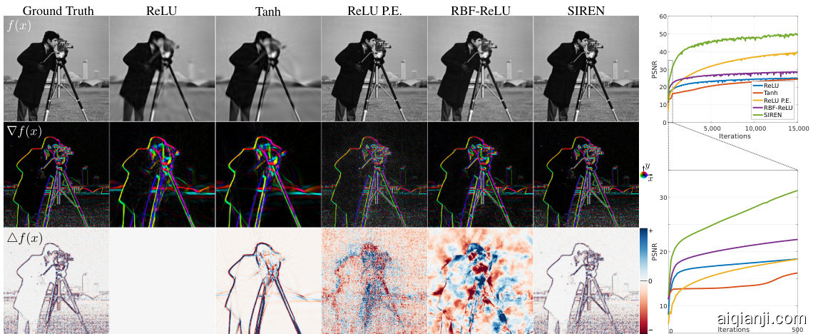
Figure 1: Comparison of different implicit network architectures fitting a ground truth image (top left). The representation is only supervised on the target image but we also show first- and second-order derivatives of the function fit in rows 2 and 3, respectively.
图 1: 不同隐式网络架构拟合真实图像(左上)的对比。该表示仅针对目标图像进行监督训练,但我们同时展示了函数拟合的一阶导数(第二行)和二阶导数(第三行)。
Neural DE Solvers. Neural networks have long been investigated in the context of solving differential equations (DEs) [36], and have previously been introduced as implicit representations for this task [37]. Early work on this topic involved simple neural network models, consisting of MLPs or radial basis function networks with few hidden layers and hyperbolic tangent or sigmoid nonlinearities [37–39]. The limited capacity of these shallow networks typically constrained results to 1D solutions or simple 2D surfaces. Modern approaches to these techniques leverage recent optimization frameworks and auto-differentiation, but use similar architectures based on MLPs. Still, solving more sophisticated equations with higher dimensionality, more constraints, or more complex geometries is feasible [40–42]. However, we show that the commonly used MLPs with smooth, non-periodic activation functions fail to accurately model high-frequency information and higher-order derivatives even with dense supervision.
神经微分方程求解器。神经网络在求解微分方程(DEs)领域的研究由来已久[36],此前已被引入作为该任务的隐式表示方法[37]。早期研究采用简单的神经网络模型,如浅层MLP或径向基函数网络,仅含少量隐藏层并使用双曲正切或Sigmoid非线性激活函数[37-39]。这些浅层网络的有限能力通常将求解范围限制在一维问题或简单二维曲面。现代方法虽然利用了最新优化框架和自动微分技术,但仍采用基于MLP的类似架构。研究表明,即使采用密集监督,常用的光滑非周期性激活函数MLP仍无法准确建模高频信息和高阶导数[40-42],不过求解更高维度、更多约束或更复杂几何形态的精密方程已成为可能。
Neural ODEs [43] are related to this topic, but are very different in nature. Whereas implicit neural representations can be used to directly solve ODEs or PDEs from supervision on the system dynamics, neural ODEs allow for continuous function modeling by pairing a conventional ODE solver (e.g., implicit Adams or Runge-Kutta) with a network that parameter ize s the dynamics of a function. The proposed architecture may be complementary to this line of work.
神经ODE (Neural ODEs) [43] 与此主题相关,但本质上有很大不同。隐式神经表示 (implicit neural representations) 可直接通过系统动力学的监督来求解ODE或PDE,而神经ODE通过将传统ODE求解器 (例如隐式Adams法或Runge-Kutta法) 与参数化函数动力学的网络相结合,实现连续函数建模。所提出的架构可能与这一研究方向具有互补性。
3 Formulation
3 公式化
Our goal is to solve problems of the form presented in Equation (1). We cast this as a feasibility problem, where a function $\Phi$ is sought that satisfies a set of $M$ constraints ${\mathcal{C}_ {m}(\mathbf{a}(\mathbf{x}),\mathbf{\dot{\Phi}}(\mathbf{\bar{x}}),\nabla\Phi(\mathbf{x}),\dots)}_{m=1}^{M}$ , each of which relate the function $\Phi$ and/or its derivatives to quantities $\mathbf{a}(\mathbf{x})$ :
我们的目标是解决如式(1)所示的这类问题。我们将其表述为一个可行性问题,即寻找满足M个约束条件${\mathcal{C}_ {m}(\mathbf{a}(\mathbf{x}),\mathbf{\dot{\Phi}}(\mathbf{\bar{x}}),\nabla\Phi(\mathbf{x}),\dots)}_{m=1}^{M}$的函数$\Phi$,每个约束条件都将函数$\Phi$和/或其导数与量$\mathbf{a}(\mathbf{x})$关联起来:
$$
\mathcal{C}_ {m}\big(\mathbf{a}(\mathbf{x}),\boldsymbol{\Phi}(\mathbf{x}),\nabla\boldsymbol{\Phi}(\mathbf{x}),\dots\big)=0,\forall\mathbf{x}\in\Omega_{m},m=1,\dots,M
$$
$$
\mathcal{C}_ {m}\big(\mathbf{a}(\mathbf{x}),\boldsymbol{\Phi}(\mathbf{x}),\nabla\boldsymbol{\Phi}(\mathbf{x}),\dots\big)=0,\forall\mathbf{x}\in\Omega_{m},m=1,\dots,M
$$
This problem can be cast in a loss function that penalizes deviations from each of the constraints on their domain $\Omega_{m}$ :
这个问题可以转化为一个损失函数,用于惩罚在域 $\Omega_{m}$ 上对每个约束条件的偏离:
$$
\mathcal{L}=\int_{\Omega}\sum_{m=1}^{M}\mathbf{1}_{\Omega_{m}}(\mathbf{x})|\mathcal{C}_{m}(\mathbf{a}(\mathbf{x}),\Phi(\mathbf{x}),\nabla\Phi(\mathbf{x}),\ldots)|d\mathbf{x},
$$
$$
\mathcal{L}=\int_{\Omega}\sum_{m=1}^{M}\mathbf{1}_{\Omega_{m}}(\mathbf{x})|\mathcal{C}_{m}(\mathbf{a}(\mathbf{x}),\Phi(\mathbf{x}),\nabla\Phi(\mathbf{x}),\ldots)|d\mathbf{x},
$$
with the indicator function $\mathbf{1}_ {\Omega_{m}}(\mathbf{x})=1$ when $\mathbf{x}\in\Omega_{m}$ and 0 when $\mathbf{x}\notin\Omega_{m}$ . In practice, the loss function is enforced by sampling $\Omega$ . A dataset $\mathbf{\textit{D}}={(\mathbf{x}_ {i},\mathbf{a}_ {i}(\mathbf{x}))}_ {i}$ is a set of tuples of coordinates $\mathbf{x}_ {i}\in\Omega$ along with samples from the quantities $\mathbf{a}(\mathbf{x}_ {i})$ that appear in the constraints. Thus, the loss in Equation (3) is enforced on coordinates $\mathbf{x}_ {i}$ sampled from the dataset, yielding the loss $\begin{array}{r}{\tilde{\mathcal{L}}=\sum_{i\in\mathcal{D}}\sum_{m=1}^{M}|\mathcal{C}_ {m}(a(\mathbf{x}_ {i}),\Phi(\mathbf{x}_ {i}),\nabla\Phi(\mathbf{x}_{i}),\ldots)|}\end{array}$ . In practice, the dataset $\mathcal{D}$ is sampled dynamically at training time, approximating $\mathcal{L}$ better as the number of samples grows, as in Monte Carlo integration.
其中指示函数 $\mathbf{1}_ {\Omega_{m}}(\mathbf{x})=1$ 当 $\mathbf{x}\in\Omega_{m}$ 时成立,否则为0。实际应用中,损失函数通过对 $\Omega$ 进行采样来实施。数据集 $\mathbf{\textit{D}}={(\mathbf{x}_ {i},\mathbf{a}_ {i}(\mathbf{x}))}_ {i}$ 是一组坐标 $\mathbf{x}_ {i}\in\Omega$ 与约束条件中出现的量 $\mathbf{a}(\mathbf{x}_ {i})$ 样本构成的元组集合。因此,方程(3)中的损失函数在数据集采样的坐标 $\mathbf{x}_ {i}$ 上实施,得到损失
。实际训练时,数据集 $\mathcal{D}$ 采用动态采样方式,随着样本数量增加,对 $\mathcal{L}$ 的近似效果会更好,这与蒙特卡洛积分原理一致。
We parameter ize functions $\Phi_{\theta}$ as fully connected neural networks with parameters $\theta$ , and solve the resulting optimization problem using gradient descent.
我们将函数 $\Phi_{\theta}$ 参数化为具有参数 $\theta$ 的全连接神经网络,并使用梯度下降法求解得到的优化问题。
3.1 Periodic Activation s for Implicit Neural Representations
3.1 隐式神经表示的周期性激活函数
We propose SIREN, a simple neural network architecture for implicit neural representations that uses the sine as a periodic activation function:
我们提出SIREN,这是一种用于隐式神经表示的简单神经网络架构,它使用正弦函数作为周期性激活函数:
$$
\Phi\left(\mathbf{x}\right)=\mathbf{W}_ {n}\left(\phi_{n-1}\circ\phi_{n-2}\circ\ldots\circ\phi_{0}\right)\left(\mathbf{x}\right)+\mathbf{b}_ {n},\quad\mathbf{x}_ {i}\mapsto\phi_{i}\left(\mathbf{x}_ {i}\right)=\sin\left(\mathbf{W}_ {i}\mathbf{x}_ {i}+\mathbf{b}_{i}\right).
$$
$$
\Phi\left(\mathbf{x}\right)=\mathbf{W}_ {n}\left(\phi_{n-1}\circ\phi_{n-2}\circ\ldots\circ\phi_{0}\right)\left(\mathbf{x}\right)+\mathbf{b}_ {n},\quad\mathbf{x}_ {i}\mapsto\phi_{i}\left(\mathbf{x}_ {i}\right)=\sin\left(\mathbf{W}_ {i}\mathbf{x}_ {i}+\mathbf{b}_{i}\right).
$$
Here, $\phi_{i}:\mathbb{R}^{M_{i}}\mapsto\mathbb{R}^{N_{i}}$ is the $i^{t h}$ layer of the network. It consists of the affine transform defined by the weight matrix $\mathbf{W}_ {i}\in\mathbb{R}^{N_{i}\times M_{i}}$ and the biases $\mathbf{b}_ {i}\in\mathbb{R}^{N_{i}}$ applied on the input $\mathbf{x}_ {i}\in\mathbb{R}^{M_{i}}$ , followed by the sine non linearity applied to each component of the resulting vector.
这里,$\phi_{i}:\mathbb{R}^{M_{i}}\mapsto\mathbb{R}^{N_{i}}$ 是网络的第 $i^{t h}$ 层。它由权重矩阵 $\mathbf{W}_ {i}\in\mathbb{R}^{N_{i}\times M_{i}}$ 和偏置 $\mathbf{b}_ {i}\in\mathbb{R}^{N_{i}}$ 定义的仿射变换组成,这些参数作用于输入 $\mathbf{x}_ {i}\in\mathbb{R}^{M_{i}}$ 上,随后对结果向量的每个分量应用正弦非线性激活函数。
Interestingly, any derivative of a SIREN is itself a SIREN, as the derivative of the sine is a cosine, i.e., a phase-shifted sine (see supplemental). Therefore, the derivatives of a SIREN inherit the properties of SIRENs, enabling us to supervise any derivative of SIREN with “complicated” signals. In our experiments, we demonstrate that when a SIREN is supervised using a constraint ${\mathcal{C}}_{m}$ involving the derivatives of $\phi$ , the function $\phi$ remains well behaved, which is crucial in solving many problems, including boundary value problems (BVPs).
有趣的是,SIREN 的任何导数本身也是 SIREN,因为正弦函数的导数是余弦函数,即相位偏移的正弦函数 (参见补充材料)。因此,SIREN 的导数继承了 SIREN 的特性,使我们能够用"复杂"信号监督 SIREN 的任何导数。在实验中,我们证明了当使用涉及 $\phi$ 导数的约束 ${\mathcal{C}}_{m}$ 监督 SIREN 时,函数 $\phi$ 仍能保持良好的行为,这对于解决包括边值问题 (BVP) 在内的许多问题至关重要。
We will show that SIRENs can be initialized with some control over the distribution of activation s, allowing us to create deep architectures. Furthermore, SIRENs converge significantly faster than baseline architectures, fitting, for instance, a single image in a few hundred iterations, taking a few seconds on a modern GPU, while featuring higher image fidelity (Fig. 1).
我们将证明SIREN可以通过初始化控制激活值的分布,从而构建深层架构。此外,SIREN的收敛速度显著快于基线架构,例如在现代GPU上仅需数百次迭代、几秒钟即可拟合单张图像,同时具备更高的图像保真度 (图 1)。
A simple example: fitting an image. Consider the case of finding the function $\Phi:\mathbb{R}^{2}\mapsto\mathbb{R}^{3},\mathbf{x}\rightarrow$ $\Phi(\mathbf{x})$ that parameter ize s a given discrete image $f$ in a continuous fashion. The image defines a dataset $\mathcal{D}={(\mathbf{x}_ {i},\bar{f}(\mathbf{x}_ {i}))}_ {i}$ of pixel coordinates $\mathbf{x}_ {i}~=~(x_{i},y_{i})$ associated with their RGB colors $f(\mathbf{x}_ {i})$ . The only constraint $\mathcal{C}$ enforces is that $\Phi$ shall output image colors at pixel coordinates, solely depending on $\Phi$ (none of its derivatives) and $\bar{f}(\mathbf{x}_ {i})$ , with the form ${\mathcal{C}}(f(\mathbf{x}_ {i}),\Phi(\mathbf{x}))~{\stackrel{\cdot}{=}}~\Phi(\mathbf{x}_ {i})-f(\mathbf{x}_ {i})$ which can be translated into the loss $\begin{array}{r}{\tilde{\mathcal{L}}=\sum_{i}|\Phi(\mathbf{x}_ {i})-f(\mathbf{x}_{i})|^{2}}\end{array}$ . In Fig. 1,
一个简单示例:图像拟合。考虑寻找函数 $\Phi:\mathbb{R}^{2}\mapsto\mathbb{R}^{3},\mathbf{x}\rightarrow$ $\Phi(\mathbf{x})$ 的情况,该函数以连续方式参数化给定的离散图像 $f$。图像定义了一个数据集 $\mathcal{D}={(\mathbf{x}_ {i},\bar{f}(\mathbf{x}_ {i}))}_ {i}$,其中包含像素坐标 $\mathbf{x}_ {i}~=~(x_{i},y_{i})$ 及其对应的 RGB 颜色 $f(\mathbf{x}_ {i})$。约束 $\mathcal{C}$ 的唯一要求是 $\Phi$ 应在像素坐标处输出图像颜色,仅取决于 $\Phi$(不包括其导数)和 $\bar{f}(\mathbf{x}_ {i})$,形式为 ${\mathcal{C}}(f(\mathbf{x}_ {i}),\Phi(\mathbf{x}))~{\stackrel{\cdot}{=}}~\Phi(\mathbf{x}_ {i})-f(\mathbf{x}_ {i})$,可转化为损失函数 $\begin{array}{r}{\tilde{\mathcal{L}}=\sum_{i}|\Phi(\mathbf{x}_ {i})-f(\mathbf{x}_{i})|^{2}}\end{array}$。在图 1 中,
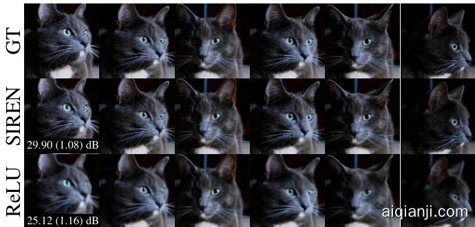
Figure 2: Example frames from fitting a video with SIREN and ReLU-MLPs. Our approach faithfully reconstructs fine details like the whiskers. Mean (and standard deviation) of the PSNR over all frames is reported.
图 2: 使用SIREN和ReLU-MLP拟合视频的示例帧。我们的方法能准确重建胡须等细微特征。报告了所有帧PSNR的平均值(及标准差)。
we fi t $\Phi_{\theta}$ using comparable network architectures with different activation functions to a natural image. We supervise this experiment only on the image values, but also visualize the gradients $\nabla f$ and Laplacians $\Delta f$ . While only two approaches, a ReLU network with positional encoding (P.E.) [5] and our SIREN, accurately represent the ground truth image $f\left(\mathbf{x}\right)$ , SIREN is the only network capable of also representing the derivatives of the signal. Additionally, we run a simple experiment where we fit a short video with 300 frames and with a resolution of $512\times512$ pixels using both ReLU and SIREN MLPs. As seen in Figure 2, our approach is successful in representing this video with an average peak signal-to-noise ratio close to $30\mathrm{dB}$ , outperforming the ReLU baseline by about 5 dB. We also show the flexibility of SIRENs by representing audio signals in the supplement.
我们使用不同激活函数的可比网络架构对自然图像拟合 $\Phi_{\theta}$。本实验仅监督图像值,但也可视化梯度 $\nabla f$ 和拉普拉斯算子 $\Delta f$。虽然只有两种方法(带位置编码(P.E.) [5]的ReLU网络和我们的SIREN)能准确表示真实图像 $f\left(\mathbf{x}\right)$,但SIREN是唯一还能表示信号导数的网络。此外,我们进行了一个简单实验,分别用ReLU和SIREN多层感知器拟合一段300帧、分辨率为 $512\times512$ 像素的短视频。如图2所示,我们的方法成功表示该视频,平均峰值信噪比接近 $30\mathrm{dB}$,比ReLU基线高出约5 dB。补充材料中还展示了SIREN表示音频信号的灵活性。
3.2 Distribution of activation s, frequencies, and a principled initialization scheme
3.2 激活值分布、频率及原则性初始化方案
We present a principled initialization scheme necessary for the effective training of SIRENs. While presented informally here, we discuss further details, proofs and empirical validation in the supplemental material. The key idea in our initialization scheme is to preserve the distribution of activation s through the network so that the final output at initialization does not depend on the number of layers. Note that building SIRENs with not carefully chosen uniformly distributed weights yielded poor performance both in accuracy and in convergence speed.
我们提出了一种必要的原则性初始化方案,用于有效训练SIRENs。虽然这里非正式地进行了介绍,但我们在补充材料中讨论了更多细节、证明和实证验证。我们初始化方案的关键思想是保持网络中激活的分布,使得初始化时的最终输出不依赖于层数。需要注意的是,使用未精心选择的均匀分布权重构建SIRENs会导致准确性和收敛速度表现不佳。
To this end, let us first consider the output distribution of a single sine neuron with the uniformly distributed input $x\sim\mathcal{U}(-1,1)$ . The neuron’s output is $y=\sin(a x+b)$ with $a,b\in\mathbb{R}$ . It can be shown that for any $a>{\frac{\pi}{2}}$ , i.e. spanning at least half a period, the output of the sine is $y\sim$ arcsine $(-1,1)$ , a special case of a U-shaped Beta distribution and independent of the choice of $b$ . We can now reason about the output distribution of a neuron. Taking the linear combination of $n$ inputs $\mathbf{x}\in\mathbb{R}^{n}$ weighted by $\mathbf{w}\in\mathbb{R}^{n}$ , its output is $y=\sin\bigl(\mathbf{w}^{T}\mathbf{x}+b\bigr)^{\circ}$ . Assuming this neuron is in the second layer, each of its inputs is arcsine distributed. When each component of w is uniformly distributed such as $w_{i}\sim\mathcal{U}(-\bar{c}/\sqrt{n},c/\sqrt{n}),c\in\mathbb{R}$ , we show (see supplemental) that the dot product converges to the normal distribution $\dot{\mathbf{w}}^{\dot{T}}\mathbf{x}\sim\mathcal{N}(0,c^{2}/6)$ as $n$ grows. Finally, feeding this normally distributed dot product through another sine is also arcsine distributed for any $c>{\sqrt{6}}$ . Note that the weights of a SIREN can be interpreted as angular frequencies while the biases are phase offsets. Thus, larger frequencies appear in the networks for weights with larger magnitudes. For $\vert\mathbf{w}^{T}\mathbf{x}\vert<\pi/4$ , the sine layer will leave the frequencies unchanged, as the sine is approximately linear. In fact, we empirically find that a sine layer keeps spatial frequencies approximately constant for amplitudes such as $|\mathbf{w}^{T}\mathbf{x}|<\pi$ , and increases spatial frequencies for amplitudes above this value2.
为此,我们首先考虑输入均匀分布 $x\sim\mathcal{U}(-1,1)$ 时单个正弦神经元的输出分布。该神经元的输出为 $y=\sin(a x+b)$,其中 $a,b\in\mathbb{R}$。可以证明,对于任意 $a>{\frac{\pi}{2}}$(即至少跨越半个周期),正弦输出服从 $y\sim$ 反正弦 $(-1,1)$ 分布——这是U型Beta分布的特例,且与 $b$ 的选择无关。
现在我们可以推导神经元的输出分布。取 $n$ 维输入 $\mathbf{x}\in\mathbb{R}^{n}$ 与权重 $\mathbf{w}\in\mathbb{R}^{n}$ 的线性组合,其输出为 $y=\sin\bigl(\mathbf{w}^{T}\mathbf{x}+b\bigr)^{\circ}$。假设该神经元位于第二层,其每个输入都服从反正弦分布。当权重分量满足 $w_{i}\sim\mathcal{U}(-\bar{c}/\sqrt{n},c/\sqrt{n}),c\in\mathbb{R}$ 时,我们证明(见补充材料)随着 $n$ 增大,点积结果收敛于正态分布 $\dot{\mathbf{w}}^{\dot{T}}\mathbf{x}\sim\mathcal{N}(0,c^{2}/6)$。最后,将这个正态分布的点积通过另一个正弦函数处理后,对于任意 $c>{\sqrt{6}}$ 仍将保持反正弦分布。
需要注意的是,SIREN网络的权重可解释为角频率,而偏置则是相位偏移。因此,权重幅值越大,网络中出现的频率越高。当 $\vert\mathbf{w}^{T}\mathbf{x}\vert<\pi/4$ 时,由于正弦函数近似线性,该层将保持频率不变。实际上,我们通过实验发现:对于 $|\mathbf{w}^{T}\mathbf{x}|<\pi$ 的振幅范围,正弦层能使空间频率保持大致恒定;而当振幅超过该阈值时,空间频率会随之增加[2]。

Figure 3: Poisson image reconstruction: An image (left) is reconstructed by fitting a SIREN, supervised either by its gradients or Laplacians (underlined in green). The results, shown in the center and right, respectively, match both the image and its derivatives well. Poisson image editing: The gradients of two images (top) are fused (bottom left). SIREN allows for the composite (right) to be reconstructed using supervision on the gradients (bottom right).
图 3: 泊松图像重建:通过拟合SIREN对图像(左)进行重建,监督信号为其梯度或拉普拉斯算子(绿色下划线标注)。如中间和右侧所示,重建结果在图像及其导数层面均实现良好匹配。泊松图像编辑:两幅图像的梯度(上)被融合(左下)。SIREN通过梯度监督实现了复合图像的重建(右下)。
Hence, we propose to draw weights with $c=6$ so that $w_{i}\sim\mathcal{U}(-\sqrt{6/n},\sqrt{6/n})$ . This ensures that the input to each sine activation is normal distributed with a standard deviation of 1. Since only a few weights have a magnitude larger than $\pi$ , the frequency throughout the sine network grows only slowly. Finally, we propose to initialize the first layer of the sine network with weights so that the sine function $\sin(\omega_{0}\cdot\mathbf{W}\mathbf{x}+\mathbf{b})$ spans multiple periods over $[-1,1]$ . We found $\omega_{0}=30$ to work well for all the applications in this work. The proposed initialization scheme yielded fast and robust convergence using the ADAM optimizer for all experiments in this work.
因此,我们建议采用 $c=6$ 来初始化权重,使得 $w_{i}\sim\mathcal{U}(-\sqrt{6/n},\sqrt{6/n})$ 。这能确保每个正弦激活的输入服从标准差为1的正态分布。由于仅有少数权重幅值超过 $\pi$ ,整个正弦网络的频率增长较为缓慢。最后,我们建议初始化正弦网络第一层的权重,使正弦函数 $\sin(\omega_{0}\cdot\mathbf{W}\mathbf{x}+\mathbf{b})$ 在 $[-1,1]$ 区间内覆盖多个周期。本研究中发现 $\omega_{0}=30$ 适用于所有应用场景。采用该初始化方案后,配合ADAM优化器在本研究所有实验中均实现了快速且稳健的收敛。
4 Experiments
4 实验
In this section, we leverage SIRENs to solve challenging boundary value problems using different types of supervision of the derivatives of $\Phi$ . We first solve the Poisson equation via direct supervision of its derivatives. We then solve a particular form of the Eikonal equation, placing a unit-norm constraint on gradients, parameter i zing the class of signed distance functions (SDFs). SIREN significantly outperforms ReLU-based SDFs, capturing large scenes at a high level of detail. We then solve the second-order Helmholtz partial differential equation, and the challenging inverse problem of full-waveform inversion. Finally, we combine SIRENs with hyper networks, learning a prior over the space of parameterized functions. All code and data will be made publicly available.
在本节中,我们利用SIREN通过不同类型的$\Phi$导数监督来解决具有挑战性的边值问题。首先通过直接监督其导数来求解泊松方程。接着求解一种特殊形式的Eikonal方程,对梯度施加单位范数约束,从而参数化有符号距离函数(SDF)的类别。SIREN显著优于基于ReLU的SDF方法,能够以高细节水平捕捉大场景。随后我们求解二阶Helmholtz偏微分方程,以及全波形反演这一具有挑战性的逆问题。最后,我们将SIREN与超网络结合,学习参数化函数空间上的先验分布。所有代码和数据都将公开提供。
4.1 Solving the Poisson Equation
4.1 求解泊松方程
We demonstrate that the proposed representation is not only able to accurately represent a function and its derivatives, but that it can also be supervised solely by its derivatives, i.e., the model is never presented with the actual function values, but only values of its first or higher-order derivatives.
我们证明所提出的表示不仅能准确表达函数及其导数,还能仅通过导数进行监督,即模型从未接触实际函数值,仅使用一阶或高阶导数值。
An intuitive example representing this class of problems is the Poisson equation. The Poisson equation is perhaps the simplest elliptic partial differential equation (PDE) which is crucial in physics
表示这类问题的一个直观例子是泊松方程。泊松方程可能是最简单的椭圆偏微分方程 (PDE) ,在物理学中至关重要

Figure 4: Shape representation. We fit signed distance functions parameterized by implicit neural representations directly on point clouds. Compared to ReLU implicit representations, our periodic activation s significantly improve detail of objects (left) and complexity of entire scenes (right).
图 4: 形状表示。我们直接在点云上拟合由隐式神经表示参数化的有符号距离函数。与ReLU隐式表示相比,我们的周期性激活函数显著提升了物体细节(左)和整体场景复杂度(右)。
and engineering, for example to model potentials arising from distributions of charges or masses. In this problem, an unknown ground truth signal $f$ is estimated from discrete samples of either its gradients $\nabla f$ or Laplacian $\Delta f=\nabla\cdot\nabla f$ as
例如在物理和工程中,用于模拟由电荷或质量分布产生的势场。该问题旨在从离散采样的梯度 $\nabla f$ 或拉普拉斯算子 $\Delta f=\nabla\cdot\nabla f$ 中估算未知的真实信号 $f$。
$$
\mathcal{L}_ {\mathrm{grad.}}=\int_{\Omega}\Vert\nabla_{\mathbf{x}}\Phi(\mathbf{x})-\nabla_{\mathbf{x}}f(\mathbf{x})\Vert d\mathbf{x},\quad\mathrm{or}\quad\mathcal{L}_ {\mathrm{lapl.}}=\int_{\Omega}\Vert\Delta\Phi(\mathbf{x})-\Delta f(\mathbf{x})\Vert d\mathbf{x}.
$$
$$
\mathcal{L}_ {\mathrm{grad.}}=\int_{\Omega}\Vert\nabla_{\mathbf{x}}\Phi(\mathbf{x})-\nabla_{\mathbf{x}}f(\mathbf{x})\Vert d\mathbf{x},\quad\mathrm{or}\quad\mathcal{L}_ {\mathrm{lapl.}}=\int_{\Omega}\Vert\Delta\Phi(\mathbf{x})-\Delta f(\mathbf{x})\Vert d\mathbf{x}.
$$
Poisson image reconstruction. Solving the Poisson equation enables the reconstruction of images from their derivatives. We show results of this approach using SIREN in Fig. 3. Supervising the implicit representation with either ground truth gradients via $\mathcal{L}_ {\mathrm{grad}}$ . or Laplacians via $\mathcal{L}_{\mathrm{lapl}}$ . successfully reconstructs the image. Remaining intensity variations are due to the ill-posedness of the problem.
泊松图像重建。通过求解泊松方程可以从导数重建图像。我们在图3中展示了使用SIREN实现这一方法的结果。通过$\mathcal{L}_ {\mathrm{grad}}$监督真实梯度,或通过$\mathcal{L}_{\mathrm{lapl}}$监督拉普拉斯算子,都能成功重建图像。剩余的强度变化是由于该问题的不适定性造成的。
Poisson image editing. Images can be seamlessly fused in the gradient domain [44]. For this purpose, $\Phi$ is supervised using $\mathcal{L}_ {\mathrm{grad}}$ . of Eq. (5), where $\nabla_{\mathbf x}f(\mathbf x)$ is a composite function of the gradients of two images $f_{1,2}\colon\nabla_{\mathbf{x}}{\tilde{f}}(\mathbf{x})=\alpha\cdot\nabla f_{1}(x)+(1-\alpha)\cdot\nabla f_{2}(x),\alpha\in[0,$ . Fig. 3 shows two images seamlessly fused with this approach.
泊松图像编辑。图像可以在梯度域中实现无缝融合[44]。为此,$\Phi$ 通过 $\mathcal{L}_ {\mathrm{grad}}$ 进行监督,如式(5)所示,其中 $\nabla_{\mathbf x}f(\mathbf x)$ 是两个图像 $f_{1,2}\colon\nabla_{\mathbf{x}}{\tilde{f}}(\mathbf{x})=\alpha\cdot\nabla f_{1}(x)+(1-\alpha)\cdot\nabla f_{2}(x),\alpha\in[0,$ 的梯度复合函数。图3展示了用该方法无缝融合的两幅图像。
4.2 Representing Shapes with Signed Distance Functions
4.2 基于符号距离函数的形状表示
Inspired by recent work on shape representation with differentiable signed distance functions (SDFs) [1, 4, 9], we fit SDFs directly on oriented point clouds using both ReLU-based implicit neural representations and SIRENs. This amounts to solving a particular Eikonal boundary value problem that constrains the norm of spatial gradients $|\nabla_{\mathbf{x}}\Phi|$ to be 1 almost everywhere. Note that ReLU networks are seemingly ideal for representing SDFs, as their gradients are locally constant and their second derivatives are 0. Adequate training procedures for working directly with point clouds were described in prior work [4, 9]. We fit a SIREN to an oriented point cloud using a loss of the form
受近期利用可微符号距离函数(SDF)进行形状表示的研究[1,4,9]启发,我们同时采用基于ReLU的隐式神经表示和SIREN直接在定向点云上拟合SDF。这相当于求解一个特定的Eikonal边值问题,该问题约束空间梯度$|\nabla_{\mathbf{x}}\Phi|$的范数在几乎所有位置都为1。值得注意的是,ReLU网络看似是表示SDF的理想选择,因为其梯度局部恒定且二阶导数为0。先前研究[4,9]已描述了直接处理点云的适当训练流程。我们通过以下形式的损失函数将SIREN拟合到定向点云:
$$
\mathcal{L}_ {\mathrm{sdf}}=\int_{\Omega}\big|\big||\nabla_{\mathbf{x}}\Phi(\mathbf{x})|-1\big|\big|d\mathbf{x}+\int_{\Omega_{0}}\left|\Phi(\mathbf{x})\right|+\big(1-\langle\nabla_{\mathbf{x}}\Phi(\mathbf{x}),\mathbf{n}(\mathbf{x})\rangle\big)d\mathbf{x}+\int_{\Omega\backslash\Omega_{0}}\psi\big(\Phi(\mathbf{x})\big)d\mathbf{x},
$$
$$
\mathcal{L}_ {\mathrm{sdf}}=\int_{\Omega}\big|\big||\nabla_{\mathbf{x}}\Phi(\mathbf{x})|-1\big|\big|d\mathbf{x}+\int_{\Omega_{0}}\left|\Phi(\mathbf{x})\right|+\big(1-\langle\nabla_{\mathbf{x}}\Phi(\mathbf{x}),\mathbf{n}(\mathbf{x})\rangle\big)d\mathbf{x}+\int_{\Omega\backslash\Omega_{0}}\psi\big(\Phi(\mathbf{x})\big)d\mathbf{x},
$$
Here, $\psi(\mathbf{x})=\exp(-\alpha\cdot|\Phi(\mathbf{x})|),\alpha\gg1$ penalizes off-surface points for creating SDF values close to 0. $\Omega$ is the whole domain and we denote the zero-level set of the SDF as $\Omega_{0}$ . The model $\Phi(x)$ is supervised using oriented points sampled on a mesh, where we require the SIREN to respect $\Phi(\mathbf{x})=0$ and its normals $\mathbf{\bar{n}}(\mathbf{x})=\bar{\nabla}f(\mathbf{x})$ . During training, each minibatch contains an equal number of points on and off the mesh, each one randomly sampled over $\Omega$ . As seen in Fig. 4, the proposed periodic activation s significantly increase the details of objects and the complexity of scenes that can be represented by these neural SDFs, parameter i zing a full room with only a single five-layer fully connected neural network. This is in contrast to concurrent work that addresses the same failure of conventional MLP architectures to represent complex or large scenes by locally decoding a discrete representation, such as a voxelgrid, into an implicit neural representation of geometry [11–13].
这里,$\psi(\mathbf{x})=\exp(-\alpha\cdot|\Phi(\mathbf{x})|),\alpha\gg1$ 通过惩罚离面点来避免生成接近0的SDF值。$\Omega$ 表示整个定义域,我们将SDF的零水平集记为 $\Omega_{0}$。模型 $\Phi(x)$ 使用网格上采样的定向点进行监督,要求SIREN网络满足 $\Phi(\mathbf{x})=0$ 及其法向量 $\mathbf{\bar{n}}(\mathbf{x})=\bar{\nabla}f(\mathbf{x})$。训练时,每个小批次包含等量的网格上和网格外点,均在 $\Omega$ 范围内随机采样。如图4所示,所提出的周期性激活函数显著提升了物体细节表现力,使得单个五层全连接神经网络就能参数化整个房间的复杂场景。这与同期研究形成鲜明对比——后者通过将离散表示(如体素网格)局部解码为几何的隐式神经表示 [11-13],来解决传统MLP架构无法表征复杂/大场景的问题。
4.3 Solving the Helmholtz and Wave Equations
4.3 求解亥姆霍兹方程和波动方程
The Helmholtz and wave equations are second-order partial differential equations related to the physical modeling of diffusion and waves. They are closely related through a Fourier-transform relationship, with the Helmholtz equation given as
亥姆霍兹方程和波动方程是与扩散和波的物理建模相关的二阶偏微分方程。它们通过傅里叶变换关系紧密联系,其中亥姆霍兹方程表示为
$$
H(m)\Phi(\mathbf{x})=-f(\mathbf{x}),\mathrm{with}H(m)=\bigl(\Delta+m(\mathbf{x})w^{2}\bigr).
$$
$$
H(m)\Phi(\mathbf{x})=-f(\mathbf{x}),\mathrm{with}H(m)=\bigl(\Delta+m(\mathbf{x})w^{2}\bigr).
$$

Figure 5: Direct Inversion: We solve the Helmholtz equation for a single point source placed at the center of a medium (green dot) with uniform wave propagation velocity (top left). The SIREN solution closely matches a principled grid solver [45] while other network architectures fail to find the correct solution. Neural Full-Waveform Inversion (FWI): A scene contains a source (green) and a circular wave velocity perturbation centered at the origin (top left). With the scene velocity known a priori, SIREN directly reconstructs a wavefield that closely matches a principled grid solver [45] (bottom left, middle left). For FWI, the velocity and wavefields are reconstructed with receiver measurements (blue dots) from sources triggered in sequence (green, red dots). The SIREN velocity model outperforms a principled FWI solver [46], accurately predicting wavefields. FWI MSE values are calculated across all wavefields and the visualized real wavefield corresponds to the green source.
图 5: 直接反演:我们在均匀波速介质(左上)中心放置单点源(绿点)求解亥姆霍兹方程。SIREN的解与基于网格的解析解[45]高度吻合,而其他网络架构无法找到正确解。神经全波形反演(FWI):场景包含一个震源(绿色)和以原点为中心的圆形波速扰动(左上)。在已知场景波速前提下,SIREN直接重建的波场与基于网格的解析解[45]高度吻合(左下,中左)。对于FWI,通过序列触发震源(绿色、红点)的接收器测量值(蓝点)重建波速和波场。SIREN波速模型优于传统FWI求解器[46],能准确预测波场。FWI均方误差值在所有波场计算得出,可视化实波场对应绿色震源。
Here, $f(\mathbf{x})$ represents a known source function, $\Phi(\mathbf{x})$ is the unknown wavefield, and the squared slowness $\dot{m}(\mathbf{\bar{x}})=1/c(\mathbf{x})^{2}$ is a function of the wave velocity $c(\mathbf{x})$ . In general, the solutions to the Helmholtz equation are complex-valued and require numerical solvers to compute. As the Helmholtz and wave equations follow a similar form, we discuss the Helmholtz equation here, with additional results and discussion for the wave equation in the supplement.
这里,$f(\mathbf{x})$ 代表已知的源函数,$\Phi(\mathbf{x})$ 是未知的波场,平方慢度 $\dot{m}(\mathbf{\bar{x}})=1/c(\mathbf{x})^{2}$ 是波速 $c(\mathbf{x})$ 的函数。一般来说,亥姆霍兹方程的解是复数值,需要数值求解器来计算。由于亥姆霍兹方程和波动方程形式相似,我们在此讨论亥姆霍兹方程,关于波动方程的更多结果和讨论见补充材料。
Solving for the wavefield. We solve for the wavefield by parameter i zing $\Phi(\mathbf{x})$ with a SIREN. To accommodate a complex-valued solution, we configure the network to output two values, interpreted as the real and imaginary parts. Training is performed on randomly sampled points $\mathbf{x}$ within the domain $\Omega={{\bf x}\in\mathbb{R}^{2}|\bar{|}{\bf x}|_ {\infty}<1}$ . The network is supervised using a loss function based on the Helmholtz equation, $\begin{array}{r}{\ddot{\mathcal{L}}_ {\mathrm{Helmholtz}}=\int_{\Omega}\lambda(\mathbf{x})|H(m)\mathring{\Phi(\mathbf{x})}+f(\mathbf{x})|\overline{{\mathbf{\rho}}}d\mathbf{x}}\end{array}$ , with $\lambda(\mathbf{x})~=~k$ , a hyper parameter, when $f(\mathbf{x})\neq0$ (corresponding to the in homogeneous contribution to the Helmholtz equation) and $\lambda(\mathbf{x})=1$ otherwise (for the homogenous part). Each minibatch contains samples from both contributions and $k$ is set so the losses are approximately equal at the beginning of training. In practice, we use a slightly modified form of Equation (7) to include the perfectly matched boundary conditions that are necessary to ensure a unique solution [45] (see supplement for details).
求解波场。我们通过用SIREN参数化$\Phi(\mathbf{x})$来求解波场。为适应复数值解,将网络配置为输出两个值,分别解释为实部和虚部。训练在域$\Omega={{\bf x}\in\mathbb{R}^{2}|\bar{|}{\bf x}|_ {\infty}<1}$内随机采样点$\mathbf{x}$上进行。网络监督使用基于亥姆霍兹方程的损失函数$\begin{array}{r}{\ddot{\mathcal{L}}_ {\mathrm{Helmholtz}}=\int_{\Omega}\lambda(\mathbf{x})|H(m)\mathring{\Phi(\mathbf{x})}+f(\mathbf{x})|\overline{{\mathbf{\rho}}}d\mathbf{x}}\end{array}$,其中当$f(\mathbf{x})\neq0$时(对应亥姆霍兹方程的非齐次项)$\lambda(\mathbf{x})~=~k$(一个超参数),否则$\lambda(\mathbf{x})=1$(对应齐次项)。每个小批量包含来自这两项的样本,且$k$的设置使训练初期损失大致相等。实践中,我们使用方程(7)的略微修改形式以包含确保唯一解所需的完美匹配边界条件[45](详见补充材料)。
Results are shown in Fig. 5 for solving the Helmholtz equation in two dimensions with spatially uniform wave velocity and a single point source (modeled as a Gaussian with $\sigma^{2}=10^{-\hat{4}}\nonumber $ ). The SIREN solution is compared with a principled solver [45] as well as other neural network solvers. All evaluated network architectures use the same number of hidden layers as SIREN but with different activation functions. In the case of the RBF network, we prepend an RBF layer with 1024 hidden units and use a tanh activation. SIREN is the only representation capable of producing a high-fidelity reconstruction of the wavefield. We also note that the tanh network has a similar architecture to recent work on neural PDE solvers [41], except we increase the network size to match SIREN.
结果如图 5 所示,展示了在二维空间中求解具有空间均匀波速和单点源 (建模为高斯分布,$\sigma^{2}=10^{-\hat{4}}\nonumber$) 的亥姆霍兹方程。SIREN 的求解结果与原理性求解器 [45] 及其他神经网络求解器进行了对比。所有评估的网络架构均采用与 SIREN 相同数量的隐藏层,但使用不同的激活函数。对于 RBF 网络,我们在前端添加了包含 1024 个隐藏单元的 RBF 层,并采用 tanh 激活函数。SIREN 是唯一能够实现波场高保真重建的表示方法。我们还注意到,tanh 网络与近期神经 PDE 求解器研究 [41] 的架构相似,只是我们扩大了网络规模以匹配 SIREN。
Neural full-waveform inversion (FWI). In many wave-based sensing modalities (radar, sonar, seismic imaging, etc.), one attempts to probe and sense across an entire domain using sparsely placed sources (i.e., transmitters) and receivers. FWI uses the known locations of sources and receivers to jointly recover the entire wavefield and other physical properties, such as permittivity, density, or wave velocity. Specifically, the FWI problem can be described as [47]
神经全波形反演 (FWI)。在许多基于波的传感模式(雷达、声纳、地震成像等)中,人们试图通过稀疏分布的源(即发射器)和接收器对整个域进行探测和感知。FWI利用已知的源和接收器位置来联合恢复整个波场以及其他物理特性,如介电常数、密度或波速。具体而言,FWI问题可描述为[47]

where there are $N$ sources, $\operatorname{III}_ {r}$ samples the wavefield at the receiver locations, and $r_{i}(x)$ models receiver data for the ith source.
存在 $N$ 个源时,$\operatorname{III}_ {r}$ 在接收器位置对波场进行采样,而 $r_{i}(x)$ 为第 $i$ 个源的接收器数据建模。
We first use a SIREN to directly solve Eq. 7 for a known wave velocity perturbation, obtaining an accurate wavefield that closely matches that of a principled solver [45] (see Fig. 5, right). Without a priori knowledge of the velocity field, FWI is used to jointly recover the wavefields and velocity. Here, we use 5 sources and place 30 receivers around the domain, as shown in Fig. 5. Using the principled solver, we simulate the receiver measurements for the 5 wavefields (one for each source) at a single frequency of $3.2\mathrm{Hz}$ , which is chosen to be relatively low for improved convergence. We pre-train SIREN to output 5 complex wavefields and a squared slowness value for a uniform velocity. Then, we optimize for the wavefields and squared slowness using a penalty method variation [47] of Eq. 8 (see the supplement for additional details). In Fig. 5, we compare to an FWI solver based on the alternating direction method of multipliers [46, 48]. With only a single frequency for the inversion, the principled solver is prone to converge to a poor solution for the velocity. As shown in Fig. 5, SIREN converges to a better velocity solution and accurate solutions for the wavefields. All reconstructions are performed or shown at $256\times256$ resolution to avoid noticeable stair-stepping artifacts in the circular velocity perturbation.
我们首先使用SIREN直接求解已知波速扰动的方程7,获得了与原理求解器[45]高度吻合的精确波场(见图5右)。在缺乏速度场先验知识的情况下,采用全波形反演(FWI)联合重建波场与速度场。如图5所示,我们布置了5个震源并在区域周边部署30个接收器。通过原理求解器,我们在单一频率3.2Hz下模拟了5个波场(每个震源对应一个波场)的接收器测量数据,该频率选择较低以提升收敛性。我们预先训练SIREN输出5个复波场和均匀速度下的平方慢度值,随后采用方程8的惩罚方法变体[47](详见补充材料)对波场和平方慢度进行优化。图5展示了与基于乘子交替方向法[46,48]的FWI求解器的对比结果。在单频反演条件下,原理求解器易收敛至较差的速度解。如图所示,SIREN能收敛至更优的速度解和精确的波场解。所有重建均在256×256分辨率下完成或展示,以避免圆形速度扰动中出现明显的阶梯状伪影。

Figure 6: Generalizing across implicit functions parameterized by SIRENs on the CelebA dataset [49]. Image inpainting results are shown for various numbers of context pixels in $O_{j}$ . tion over SIREN representations is at least equally as powerful as generalization over images.
图 6: 在CelebA数据集[49]上通过SIREN参数化的隐函数泛化效果。展示了不同上下文像素数量$O_{j}$下的图像修复结果。基于SIREN表示的泛化能力至少与基于图像的泛化能力相当。
4.4 Learning a Space of Implicit Functions
4.4 学习隐函数空间
A powerful concept that has emerged for implicit representations is to learn priors over the space of functions that define them [1, 2, 10]. Here we demonstrate that the function space parameterized by SIRENs also admits the learning of powerful priors. Each of these SIRENs $\Phi_{j}$ are fully defined by their parameters $\pmb{\theta}_ {j}\in\mathbb{R}^{l}$ . Assuming that all parameters $\theta_{j}$ of a class exist in a $k$ -dimensional subspace of $\mathbb{R}^{l}$ , $k<l$ , then these parameters can be well modeled by latent code vectors in $\mathbf{z}\in\mathbb{R}^{k}$ . Like in neural processes [50–52], we condition these latent code vectors on partial observations of the signal $O\in\mathbb{R}^{m}$ through an encoder
隐式表示领域出现的一个强大概念,是学习定义这些函数的函数空间先验 [1, 2, 10]。本文证明,由SIRENs参数化的函数空间同样支持学习强大的先验。每个SIREN $\Phi_{j}$ 完全由其参数 $\pmb{\theta}_ {j}\in\mathbb{R}^{l}$ 定义。假设某类别的所有参数 $\theta_{j}$ 都存在于 $\mathbb{R}^{l}$ 的 $k$ 维子空间 ($k<l$) 中,那么这些参数可以通过潜在编码向量 $\mathbf{z}\in\mathbb{R}^{k}$ 很好地建模。类似于神经过程 [50–52],我们通过编码器将这些潜在编码向量与信号的部分观测 $O\in\mathbb{R}^{m}$ 相关联。
$$
C:\mathbb{R}^{m}\rightarrow\mathbb{R}^{k},\quad O_{j}\mapsto C(O_{j})=\mathbf{z}_{j},
$$
$$
C:\mathbb{R}^{m}\rightarrow\mathbb{R}^{k},\quad O_{j}\mapsto C(O_{j})=\mathbf{z}_{j},
$$
and use a ReLU hyper network [53], to map the latent code to the weights of a SIREN, as in [10]:
并使用ReLU超网络[53],将潜在代码映射到SIREN的权重,如[10]所述:
$$
\Psi:\mathbb{R}^{k}\rightarrow\mathbb{R}^{l},\quad\mathbf{z}_ {j}\mapsto\Psi(\mathbf{z}_ {j})=\pmb{\theta}_{j}.
$$
$$
\Psi:\mathbb{R}^{k}\rightarrow\mathbb{R}^{l},\quad\mathbf{z}_ {j}\mapsto\Psi(\mathbf{z}_ {j})=\pmb{\theta}_{j}.
$$
We replicated the experiment from [50] on the CelebA dataset [49] using a set encoder. Additionally, we show results using a convolutional neural network encoder which operates on sparse images. Interestingly, this improves the quantitative and qualitative performance on the inpainting task.
我们使用集合编码器在CelebA数据集[49]上复现了文献[50]的实验。此外,我们还展示了基于稀疏图像的卷积神经网络编码器结果。值得注意的是,该方法在图像修复任务中实现了定量和定性性能的双重提升。
At test time, this enables reconstruction from sparse pixel observations, and, thereby, inpainting. Fig. 6 shows test-time reconstructions from a varying number of pixel observations. Note that these inpainting results were all generated using the same model, with the same parameter val- ues. Tab. 1 reports a quantitative comparison to [50], demonstrating that generaliza
在测试时,这能够实现从稀疏像素观测中进行重建,从而进行图像修复。图6展示了基于不同数量像素观测的测试时重建结果。请注意,这些修复结果均使用同一模型生成,且参数值保持不变。表1提供了与[50]的定量比较,表明泛化
Table 1: Quantitative comparison to Conditional Neural Processes [50] (CNPs) on the $32\times32$ CelebA test set. Metrics are reported in pixel-wise mean squared error.
| Number of Context Pixels | 10 | 100 | 1000 |
| CNP [50] | 0.039 | 0.016 | 0.009 |
| Set Encoder + Hypernet. | 0.035 | 0.013 | 0.009 |
| CNN Encoder + Hypernet. | 0.033 | 0.009 | 0.008 |
表 1: 在 $32\times32$ CelebA 测试集上与条件神经过程 [50] (CNPs) 的定量比较。指标以像素级均方误差报告。
| 上下文像素数量 | 10 | 100 | 1000 |
|---|---|---|---|
| CNP [50] | 0.039 | 0.016 | 0.009 |
| 集合编码器 + 超网络 | 0.035 | 0.013 | 0.009 |
| CNN 编码器 + 超网络 | 0.033 | 0.009 | 0.008 |
5 Discussion and Conclusion
5 讨论与结论
The question of how to represent a signal is at the core of many problems across science and engineering. Implicit neural representations may provide a new tool for many of these by offering a number of potential benefits over conventional continuous and discrete representations. We demonstrate that periodic activation functions are ideally suited for representing complex natural signals and their derivatives using implicit neural representations. We also prototype several boundary value problems that our framework is capable of solving robustly. There are several exciting avenues for future work, including the exploration of other types of inverse problems and applications in areas beyond implicit neural representations, for example neural ODEs [43].
如何表示信号的问题是科学和工程领域许多问题的核心。隐式神经表示 (implicit neural representations) 可能为其中许多问题提供新工具,相比传统连续和离散表示具有多项潜在优势。我们证明周期激活函数特别适合用隐式神经表示来建模复杂自然信号及其导数。我们还构建了多个边界值问题原型,验证了该框架的稳健求解能力。未来工作存在多个激动人心的方向,包括探索其他类型的逆问题以及隐式神经表示之外的领域应用,例如神经常微分方程 (neural ODEs) [43]。
With this work, we make important contributions to the emerging field of implicit neural representation learning and its applications.
通过这项工作,我们对新兴的隐式神经表示学习(implicit neural representation learning)领域及其应用做出了重要贡献。
Broader Impact
更广泛的影响
The proposed SIREN representation enables accurate representations of natural signals, such as images, audio, and video in a deep learning framework. This may be an enabler for downstream tasks involving such signals, such as classification for images or speech-to-text systems for audio. Such applications may be leveraged for both positive and negative ends. SIREN may in the future further enable novel approaches to the generation of such signals. This has potential for misuse in impersonating actors without their consent. For an in-depth discussion of such so-called DeepFakes, we refer the reader to a recent review article on neural rendering [17].
提出的SIREN表征方法能够精准表示深度学习框架中的自然信号(如图像、音频和视频)。这为涉及此类信号的下游任务(如图像分类或音频语音转文字系统)提供了技术基础。此类应用既可能被正向利用,也可能遭负面滥用。未来SIREN可能进一步推动此类信号生成的新方法,但存在未经授权模仿演员行为的潜在滥用风险。关于这类"深度伪造(DeepFakes)"的深入讨论,建议读者参阅神经渲染领域的最新综述文章[17]。
Acknowledgments and Disclosure of Funding
致谢与资金披露声明
Vincent Sitzmann, Alexander W. Bergman, and David B. Lindell were supported by a Stanford Graduate Fellowship. Julien N. P. Martel was supported by a Swiss National Foundation (SNF) Fellowship (P2EZP2 181817). Gordon Wetzstein was supported by an NSF CAREER Award (IIS 1553333), a Sloan Fellowship, and a PECASE from the ARO.
Vincent Sitzmann、Alexander W. Bergman 和 David B. Lindell 获得了斯坦福研究生奖学金的支持。Julien N. P. Martel 获得了瑞士国家基金会 (SNF) 奖学金 (P2EZP2 181817) 的支持。Gordon Wetzstein 获得了美国国家科学基金会 CAREER 奖 (IIS 1553333)、斯隆研究奖学金和美国陆军研究办公室 (ARO) 的 PECASE 奖支持。
References
参考文献
Implicit Neural Representations with Periodic Activation Functions
基于周期性激活函数的隐式神经表示
–Supplementary Material–
–补充材料–
Vincent Sitzmann∗ sitzmann@cs.stanford.edu
Vincent Sitzmann∗ sitzmann@cs.stanford.edu
Julien N. P. Martel∗ jnmartel@stanford.edu
Julien N. P. Martel∗ jnmartel@stanford.edu
Alexander W. Bergman awb@stanford.edu
Alexander W. Bergman awb@stanford.edu
David B. Lindell lindell@stanford.edu
David B. Lindell lindell@stanford.edu
Gordon Wetzstein gordon.wetzstein@stanford.edu
Gordon Wetzstein gordon.wetzstein@stanford.edu
Stanford University vsitzmann.github.io/siren/
斯坦福大学 vsitzmann.github.io/siren/
Contents
目录
1 Initialization and Distribution of Activation s 3
1 激活 s 3 的初始化与分布
Evaluating the Gradient of a SIREN is Evaluating another SIREN 6
评估SIREN的梯度即评估另一个SIREN 6
4 Representing Shapes with Signed Distance Functions 9
4 基于符号距离函数 (Signed Distance Function) 的形状表示 9
5 Solving the Helmholtz and Wave Equations 10
5 求解亥姆霍兹方程和波动方程 10
6 Application to Image Processing 13
6 图像处理应用 13
Representing Video 16
视频表示 16
7.1 Reproducibility & Implementation Details 16
7.1 可复现性与实现细节 16
9 Learning a Space of Implicit Functions 18
9 学习隐函数空间 18
10 References 21
10 参考文献 21
1 Initialization and Distribution of Activation s
1 激活的初始化和分布
1.1 Informal statement
1.1 非正式声明
Initialization schemes have been shown to be crucial in the training procedure of deep neural networks [20, 18]. Here, we propose an initialization scheme for SIREN that preserves the distribution of activation s through its layers and thus allows us to build deep architectures.
初始化方案已被证明在深度神经网络训练过程中至关重要 [20, 18]。本文提出了一种适用于SIREN的初始化方案,该方案能保持各层激活值的分布特性,从而支持构建深层架构。
Statement of the initialization scheme. We propose to draw weights according to a uniform distribution $W\sim\mathcal{U}(-\sqrt{6/\mathrm{fan_{-}i}}$ n, $\sqrt{6/\mathrm{fan_{-}i n}})$ . We claim that this leads to the input of each sine activation being Gauss-Normal distributed, and the output of each sine activation approximately arcsine-distributed with a standard deviation of 0.5. Further, we claim that the form as well as the moments of these distributions do not change as the depth of the network grows.
初始化方案的声明。我们提出按照均匀分布 $W\sim\mathcal{U}(-\sqrt{6/\mathrm{fan_{-}i}}$ n, $\sqrt{6/\mathrm{fan_{-}i n}})$ 来抽取权重。我们声称,这将导致每个正弦激活的输入呈高斯正态分布,而每个正弦激活的输出近似服从标准差为0.5的反正弦分布。此外,我们还声称这些分布的形式和矩不会随着网络深度的增加而改变。
Overview of the proof. Our initialization scheme relies on the fact that if the input to a neuron in a layer is distributed the same way as its output, then by a simple recursive argument we can see that the distributions will be preserved throughout the network.
证明概述。我们的初始化方案基于这样一个事实:如果某层神经元的输入分布与其输出分布相同,那么通过简单的递归论证可以看出,这种分布将在整个网络中保持不变。
Hence, we consider an input in the interval $[-1,1]$ . We assume it is drawn uniformly at random, since we interpret it as a “normalized coordinate" in our applications. We first show in Lemma 1.1, that pushing this input through a sine non linearity yields an arcsine distribution. The second layer (and, as we will show, all following layers), computes a linear combination of such arcsine distributed outputs (of known variance, Lemma 1.3). Following Lindeberg’s condition for the central limit theorem, this linear combination will be normal distributed Lemma 1.5, with a variance that can be calculated using the variance of the product of random variables (Lemma 1.4). It remains to show that pushing a Gaussian distribution through the sine non linearity again yields an arcsine distributed output Lemma 1.6, and thereby, we may apply the same argument to the distributions of activation s of the following layers.
因此,我们考虑在区间 $[-1,1]$ 内的输入。由于将其视为应用中的"归一化坐标",我们假设该输入是均匀随机采样的。首先在引理 1.1 中证明:将该输入通过正弦非线性变换会得到反正弦分布。第二层(以及后续所有层)计算的是此类已知方差(引理 1.3)的反正弦分布输出的线性组合。根据中心极限定理的林德伯格条件,该线性组合将服从正态分布(引理 1.5),其方差可通过随机变量乘积的方差(引理 1.4)计算得出。最后证明将高斯分布再次通过正弦非线性变换仍会产生反正弦分布输出(引理 1.6),从而可将相同论证应用于后续层激活值的分布。
We formally present the lemmas and their proof in the next section before formally stating the initialization scheme and proving it in Section 1.3. We show empirically that the theory predicts very well the behaviour of the initialization scheme in Section 1.4.
我们将在下一节正式提出引理及其证明,然后在第1.3节正式陈述初始化方案并给出证明。第1.4节将通过实验证明该理论能很好地预测初始化方案的行为。
1.2 Preliminary results
1.2 初步结果
First let us note that the sine function is periodic, of period $2\pi$ and odd: $\sin(-x)=-\sin(x)$ , i.e. it is symmetric with respect to the origin. Since we are interested in mapping “coordinates” through SIREN, we will consider an input as a random variable $X$ uniformly distributed in [-1,1]. We will thus study, without loss of generality, the frequency scaled SIREN that uses the activation $\sin({\frac{\pi}{2}}x)$ . Which is half a period (note that the distribution does not change on a full period, it is “just” considering twice the half period).
首先我们注意到正弦函数具有周期性,周期为 $2\pi$ 且为奇函数:$\sin(-x)=-\sin(x)$ ,即关于原点对称。由于我们关注的是通过SIREN映射"坐标",因此将输入视为在[-1,1]区间均匀分布的随机变量 $X$ 。不失一般性地,我们将研究使用激活函数 $\sin({\frac{\pi}{2}}x)$ 的频率缩放版SIREN。这相当于半个周期(注意在完整周期上分布不变,相当于将半个周期延长一倍)。
Definition 1.1. The arcsine distribution is defined for a random variable $X$ by its cumulative distribution function $(C D F)~F_{X}$ such as
定义 1.1. 对于随机变量 $X$ ,其反正弦分布由累积分布函数 (CDF) $F_{X}$ 定义如下
$$
X\sim\arcsin(a,b),w i t h C D F;F_{X}(x)={\frac{2}{\pi}}\arcsin\left({\sqrt{\frac{x-a}{b-a}}}\right),w i t h b>a.
$$
$$
X\sim\arcsin(a,b),w i t h C D F;F_{X}(x)={\frac{2}{\pi}}\arcsin\left({\sqrt{\frac{x-a}{b-a}}}\right),w i t h b>a.
$$
Lemma 1.1. Given $X\sim\mathcal{U}(-1,1)$ , and $\begin{array}{r}{Y=\sin\left(\frac{\pi}{2}X\right)}\end{array}$ we have $Y\sim\arcsin(-1,1)$ .
引理 1.1. 给定 $X\sim\mathcal{U}(-1,1)$ ,且 $\begin{array}{r}{Y=\sin\left(\frac{\pi}{2}X\right)}\end{array}$ ,则有 $Y\sim\arcsin(-1,1)$ 。
Proof. The cumulative distribution function (CDF) $F_{X}(x)=\mathbb{P}(X\leq x)$ is defined, for a random variable that admits a continuous probability density function (PDF), $f$ as the integral $F_{X}(x)=$ $\textstyle\int_{-\infty}^{x}f(t)d t$ . Hence, for the uniform distribution $\mathcal{U}(-1,1)$ which is $f(x)={\frac{1}{2}}$ over the interval $[-1,1]$ and 0 everywhere else, it is easy to show that: $\begin{array}{r}{F_{X}(x)=\frac{1}{2}x+\frac{1}{2}}\end{array}$ .
证明。对于允许连续概率密度函数 (PDF) $f$ 的随机变量,累积分布函数 (CDF) $F_{X}(x)=\mathbb{P}(X\leq x)$ 定义为积分 $F_{X}(x)=$ $\textstyle\int_{-\infty}^{x}f(t)d t$。因此,对于在区间 $[-1,1]$ 上为 $f(x)={\frac{1}{2}}$ 而在其他位置为 0 的均匀分布 $\mathcal{U}(-1,1)$,容易证明:$\begin{array}{r}{F_{X}(x)=\frac{1}{2}x+\frac{1}{2}}\end{array}$。
We are interested in the distribution of the output $\begin{array}{r}{Y=\sin\left(\frac{\pi}{2}X\right)}\end{array}$ . Noting that $\sin\left({\frac{\pi}{2}}\right)$ is bijective on $[-1,1]$ , we have
我们关注输出 $Y=\sin\left(\frac{\pi}{2}X\right)$ 的分布。注意到 $\sin\left({\frac{\pi}{2}}\right)$ 在 $[-1,1]$ 上是双射的,因此有
$$
F_{Y}(y)=\mathbb{P}(\sin\left({\frac{\pi}{2}}X\right)\leq y)=\mathbb{P}(X\leq{\frac{2}{\pi}}\arcsin y)=F_{X}({\frac{2}{\pi}}\arcsin y),
$$
$$
F_{Y}(y)=\mathbb{P}(\sin\left({\frac{\pi}{2}}X\right)\leq y)=\mathbb{P}(X\leq{\frac{2}{\pi}}\arcsin y)=F_{X}({\frac{2}{\pi}}\arcsin y),
$$
Substituting the CDF $F_{X}$ , noting it is the uniform distribution which has a compact support (this is [-1,1]), we have
将累积分布函数 $F_{X}$ 代入(注意这是一个具有紧支撑的均匀分布(即[-1,1]区间)后可得
$$
F_{Y}(y)={\frac{1}{\pi}}\arcsin y+{\frac{1}{2}}.
$$
$$
F_{Y}(y)={\frac{1}{\pi}}\arcsin y+{\frac{1}{2}}.
$$
Using the identity arcsin $\scriptstyle{\sqrt{x}}={\frac{1}{2}}\arcsin(2x-1)+{\frac{\pi}{4}}$ , we conclude:
利用恒等式 arcsin $\scriptstyle{\sqrt{x}}={\frac{1}{2}}\arcsin(2x-1)+{\frac{\pi}{4}}$ ,我们得出:
$$
F_{Y}(y)\sim\arcsin(-1,1).
$$
$$
F_{Y}(y)\sim\arcsin(-1,1).
$$
The PDF can be found, deriving the cdf: $\begin{array}{r}{f_{Y}(y)=\frac{d}{d y}F_{Y}(y)=\frac{1}{\pi}\frac{1}{\sqrt{1-y^{2}}}}\end{array}$
可在PDF中找到,推导累积分布函数:$\begin{array}{r}{f_{Y}(y)=\frac{d}{d y}F_{Y}(y)=\frac{1}{\pi}\frac{1}{\sqrt{1-y^{2}}}}\end{array}$
Lemma 1.2. The variance of $m X+n$ with $X$ a random variable and $m\in\mathbb{R}_{/0}^{+},n\in\mathbb{R}$ R/+0, n ∈ R is Var[mX + $n]=m^{2}\mathrm{Var}[X]$ .
引理 1.2. 设 $X$ 为随机变量,$m\in\mathbb{R}_{/0}^{+}$,$n\in\mathbb{R}$,则 $mX+n$ 的方差为 $\mathrm{Var}[mX+n]=m^{2}\mathrm{Var}[X]$。
Proof. For any random variable with a continuous pdf $f_{X}$ , its expectation is defined as $\operatorname{E}[X]=$ $\textstyle\int_{-\infty}^{\infty}f_{X}(x)d x$ . The variance is defined as $\operatorname{Var}[X]=\operatorname{E}[(X-\operatorname{E}[X])^{2}]=\operatorname{E}[X^{2}]-\operatorname{E}[X]^{2}$ . Thus, we have $\mathrm{Var}[m X+n]=\mathrm{E}[(m X+n)^{2}]-\mathrm{E}[m X+n]^{2}=\mathrm{E}[m^{2}X^{2}+2m n X+n^{2}]-(m\mathrm{E}[X]+n)^{2}=0.$ = $m^{2}(\mathrm{E}[X^{2}]-\mathrm{E}[X^{2})=\stackrel{.}{m}^{2}\mathrm{Var}[X]$ .口
证明。对于任何具有连续概率密度函数 $f_{X}$ 的随机变量,其期望定义为 $\operatorname{E}[X]=\textstyle\int_{-\infty}^{\infty}f_{X}(x)dx$。方差定义为 $\operatorname{Var}[X]=\operatorname{E}[(X-\operatorname{E}[X])^{2}]=\operatorname{E}[X^{2}]-\operatorname{E}[X]^{2}$。因此,我们有 $\mathrm{Var}[m X+n]=\mathrm{E}[(m X+n)^{2}]-\mathrm{E}[m X+n]^{2}=\mathrm{E}[m^{2}X^{2}+2m n X+n^{2}]-(m\mathrm{E}[X]+n)^{2}=0.$ = $m^{2}(\mathrm{E}[X^{2}]-\mathrm{E}[X^{2})=\stackrel{.}{m}^{2}\mathrm{Var}[X]$。
Lemma 1.3. The variance of $X\sim\arcsin(a,b)$ is $\begin{array}{r}{\mathrm{Var}[X]=\frac{1}{8}(b-a)^{2}.}\end{array}$ .
引理 1.3. 服从 $X\sim\arcsin(a,b)$ 分布的随机变量方差为 $\begin{array}{r}{\mathrm{Var}[X]=\frac{1}{8}(b-a)^{2}.}\end{array}$。
Proof. First we prove that if $Z\sim\arcsin(0,1)$ then $\begin{array}{r}{\mathrm{Var}[Z]=\frac{1}{8}}\end{array}$ . We have $\begin{array}{r}{\operatorname{E}[Z]={\frac{1}{2}}}\end{array}$ by symmetry, and $\begin{array}{r}{\operatorname{Var}[Z]=\operatorname{E}[Z^{2}]-\operatorname{E}[Z]^{2}=\operatorname{E}[Z^{2}]-{\frac{1}{4}}}\end{array}$ . Remains to compute:
证明。首先我们证明如果 $Z\sim\arcsin(0,1)$ ,那么 $\begin{array}{r}{\mathrm{Var}[Z]=\frac{1}{8}}\end{array}$ 。由对称性可得 $\begin{array}{r}{\operatorname{E}[Z]={\frac{1}{2}}}\end{array}$ ,且 $\begin{array}{r}{\operatorname{Var}[Z]=\operatorname{E}[Z^{2}]-\operatorname{E}[Z]^{2}=\operatorname{E}[Z^{2}]-{\frac{1}{4}}}\end{array}$ 。接下来需要计算:
$$
\operatorname{E}[Z^{2}]=\int_{0}^{1}z^{2}\cdot{\frac{1}{\pi{\sqrt{z(1-z)}}}}d z={\frac{2}{\pi}}\int_{0}^{1}{\frac{t^{4}}{\sqrt{1-t^{2}}}}d t={\frac{2}{\pi}}\int_{0}^{\pi/2}\sin^{4}u d u={\frac{3}{8}},
$$
$$
\operatorname{E}[Z^{2}]=\int_{0}^{1}z^{2}\cdot{\frac{1}{\pi{\sqrt{z(1-z)}}}}d z={\frac{2}{\pi}}\int_{0}^{1}{\frac{t^{4}}{\sqrt{1-t^{2}}}}d t={\frac{2}{\pi}}\int_{0}^{\pi/2}\sin^{4}u d u={\frac{3}{8}},
$$
using a first change of variable: $z=t^{2}$ , $d z=2t d t$ and then a second change of variable $t=$ $\sin(u),d t=\cos(u)d u$ . The integral of $\sin^{4}(u)$ is calculated remarking it is $(s i\bar{n}^{2}(u))^{2}$ , and using the formulas of the double angle: $\cos(2u)=2\cos^{2}(u)-1=1-2\sin^{2}(u)$ .
使用第一次变量替换:$z=t^{2}$,$d z=2t d t$,然后进行第二次变量替换$t=\sin(u)$,$d t=\cos(u)d u$。计算$\sin^{4}(u)$的积分时,注意到它可以表示为$(s i\bar{n}^{2}(u))^{2}$,并利用二倍角公式:$\cos(2u)=2\cos^{2}(u)-1=1-2\sin^{2}(u)$。
Second, we prove that if $X\sim\arcsin(\alpha,\beta)$ then the linear combination $m X+n\sim\mathrm{Arcsin}(\alpha m+$ $n,\beta m+n)$ with $m\in\mathbb{R}_{/0},n\in\mathbb{R}$ , (using the same method as in Lemma 1.1 with $Y=m X+n)$ ).
其次,我们证明若 $X\sim\arcsin(\alpha,\beta)$,则线性组合 $m X+n\sim\mathrm{Arcsin}(\alpha m+$ $n,\beta m+n)$ 其中 $m\in\mathbb{R}_{/0},n\in\mathbb{R}$ (采用与引理1.1相同的方法,令 $Y=m X+n)$ )。
Posing $X=m Z+n$ and using $n=a$ and $m=b-a$ , we have $X\sim\arcsin(m\cdot0+n,m\cdot1+n)=$ $\arcsin(a,b)$ . Finally, $\operatorname{Var}[X]{\stackrel{.}{=}}\operatorname{Var}[m\cdot Z+n]=m^{2}\cdot\operatorname{Var}[Z]=(b-a)^{2}\cdot{\frac{1}{8}}$ (Lemma 1.2).
设定 $X=m Z+n$,并使用 $n=a$ 和 $m=b-a$,可得 $X\sim\arcsin(m\cdot0+n,m\cdot1+n)=$ $\arcsin(a,b)$。最终,$\operatorname{Var}[X]{\stackrel{.}{=}}\operatorname{Var}[m\cdot Z+n]=m^{2}\cdot\operatorname{Var}[Z]=(b-a)^{2}\cdot{\frac{1}{8}}$(引理 1.2)。
Lemma 1.4. For two independent random variables $X$ and $Y$
引理 1.4. 对于两个独立随机变量 $X$ 和 $Y$
$$
\operatorname{Var}[X\cdot Y]=\operatorname{Var}[X]\cdot\operatorname{Var}[Y]+\operatorname{E}[Y]^{2}\cdot\operatorname{Var}[X]+\operatorname{E}[X]^{2}\cdot\operatorname{Var}[Y].
$$
$$
\operatorname{Var}[X\cdot Y]=\operatorname{Var}[X]\cdot\operatorname{Var}[Y]+\operatorname{E}[Y]^{2}\cdot\operatorname{Var}[X]+\operatorname{E}[X]^{2}\cdot\operatorname{Var}[Y].
$$
Proof. See [19].
证明。参见[19]。
Theorem 1.5. Central Limit Theorem with Lindeberg’s sufficient condition. Let $X_{k}$ , $k\in\mathbb{N}b e$ independent random variables with expected values $\operatorname{E}[X_{k}]=\mu_{k}$ and variances $\mathrm{Var}[X_{k}]=\sigma_{k}$ . Posing $\begin{array}{r}{s_{n}^{2}=\sum_{k=1}^{n}\sigma_{k}^{2}}\end{array}$ . If the $X_{k}$ statisfy the Lindenberg condition:
定理 1.5. 带Lindeberg充分条件的中心极限定理。设$X_{k}$,$k\in\mathbb{N}b e$为独立随机变量,期望值$\operatorname{E}[X_{k}]=\mu_{k}$,方差$\mathrm{Var}[X_{k}]=\sigma_{k}$。令$\begin{array}{r}{s_{n}^{2}=\sum_{k=1}^{n}\sigma_{k}^{2}}\end{array}$。若$X_{k}$满足Lindenberg条件:
$$
\operatorname*{lim}_ {n\to\infty}{\frac{1}{s_{n}^{2}}}\sum_{k=1}^{n}\operatorname{E}[(X_{k}-\mu_{k})^{2}\cdot\mathbf{1}(|X_{k}-\mu_{k}|>\epsilon s_{n})]=0
$$
$$
\operatorname*{lim}_ {n\to\infty}{\frac{1}{s_{n}^{2}}}\sum_{k=1}^{n}\operatorname{E}[(X_{k}-\mu_{k})^{2}\cdot\mathbf{1}(|X_{k}-\mu_{k}|>\epsilon s_{n})]=0
$$
$\forall\epsilon>0$ , then the Central Limit Theorem (CLT) holds. That is,
$\forall\epsilon>0$,则中心极限定理 (CLT) 成立。即
$$
S_{n}={\frac{1}{s_{n}}}\sum_{k=1}^{n}(X_{k}-\mu_{k}),
$$
$$
S_{n}={\frac{1}{s_{n}}}\sum_{k=1}^{n}(X_{k}-\mu_{k}),
$$
converges in distribution to the standard normal distribution as $n\to\infty$ .
当 $n\to\infty$ 时依分布收敛于标准正态分布。
Proof. See [26, 2].
证明。参见 [26, 2]。
Lemma 1.6. Given a Gaussian distributed random variable $X\sim{\mathcal{N}}(0,1)$ and $\begin{array}{r}{Y=\sin{\frac{\pi}{2}}X}\end{array}$ we have $Y\sim\arcsin(-1,1)$ .
引理 1.6. 给定高斯分布随机变量 $X\sim{\mathcal{N}}(0,1)$ 和 $\begin{array}{r}{Y=\sin{\frac{\pi}{2}}X}\end{array}$ ,则有 $Y\sim\arcsin(-1,1)$ 。
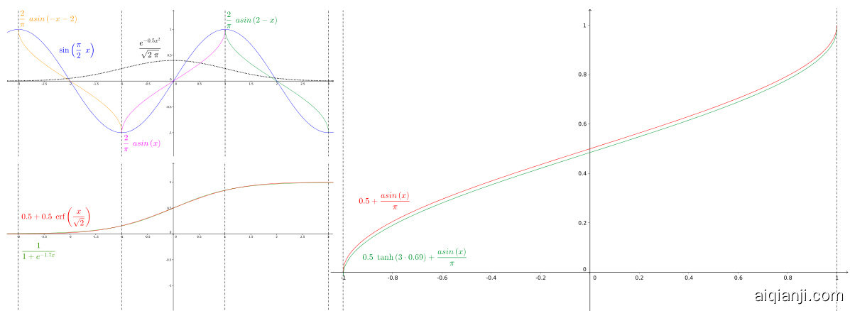
Figure 1: Top left: A plot of the standard normal distribution on $[-3,3]$ as well as the graph of $y=\sin{\frac{\pi}{2}}x$ and its three reciprocal bijections $y={\textstyle{\frac{2}{\pi}}}\arcsin(-\dot{x}-2)$ , $y={\frac{2}{\pi}}\arcsin{\bar{x}}$ and $\begin{array}{r}{y={\frac{2}{\pi}}\arcsin(2-x)}\end{array}$ covering the interval $[-3,3]$ in which $99.7%$ of the probability mass of the standard normal distribution lies. Bottom left: Plot of the approximation of the CDF of the standard normal with a logistic function. Right: Comparison of the theoretically derived CDF of the output of a sine non linearity (green) and the ground-truth Arcsine CDF (red), demonstrating that a standard normal distributed input fed to a sine indeed yields an approximately Arcsine distributed output.
图 1: 左上: 标准正态分布在 $[-3,3]$ 区间内的曲线图,以及 $y=\sin{\frac{\pi}{2}}x$ 及其三个倒数双射函数 $y={\textstyle{\frac{2}{\pi}}}\arcsin(-\dot{x}-2)$ 、 $y={\frac{2}{\pi}}\arcsin{\bar{x}}$ 和 $\begin{array}{r}{y={\frac{2}{\pi}}\arcsin(2-x)}\end{array}$ 的图形,覆盖了标准正态分布99.7%概率质量的区间。左下: 用逻辑函数近似标准正态分布的累积分布函数(CDF)的曲线图。右: 理论推导的正弦非线性输出CDF(绿色)与真实Arcsine CDF(红色)的对比,表明标准正态分布输入通过正弦函数确实产生近似Arcsine分布的输出。
Proof. For a random variable $X$ normally distributed we can approximate the CDF of its normal distribution with the logistic function, as in [10]:
证明。对于一个服从正态分布的随机变量 $X$ ,我们可以用逻辑函数近似其正态分布的累积分布函数 (CDF) ,如 [10] 所示:

with $\alpha=1.702$ and $\beta=0.690$ . Similar to the proof of Lemma (1.1), we are looking for the CDF of the random variable $Y\sim\sin\left({\frac{\pi}{2}}X\right)$ . However, the normal distribution does not have compact support. This infinite support yields an infinite series describing the CDF of Y .
其中 $\alpha=1.702$ 且 $\beta=0.690$。类似于引理 (1.1) 的证明,我们寻找随机变量 $Y\sim\sin\left({\frac{\pi}{2}}X\right)$ 的累积分布函数 (CDF)。然而,正态分布不具备紧支撑性。这种无限支撑会导致描述 Y 的 CDF 的无穷级数。
Hence, we make a second approximation that consists in approximating the CDF of Y on the interval $[-3,3]$ . Because $X\sim{\mathcal{N}}(0,1)$ , we know that $99.7%$ of the probability mass of $X$ lies on the compact set $[-3,3]$ . Thus, ignoring the other contributions, we have:
因此,我们做出第二个近似,即在区间 $[-3,3]$ 上近似 Y 的累积分布函数 (CDF)。由于 $X\sim{\mathcal{N}}(0,1)$,我们知道 $X$ 的概率质量有 $99.7%$ 位于紧集 $[-3,3]$ 上。于是忽略其他部分贡献后,可得:
$$
\begin{array}{l}{{F_{Y}(y)=\mathbb{P}(\sin\left(\displaystyle\frac{\pi}{2}X\right)\leq y)}}\ {{{}~=F_{X}(3)-F_{X}\bigl(2-\displaystyle\frac{2}{\pi}\arcsin{x}\bigr)+F_{X}\bigl(\displaystyle\frac{2}{\pi}\arcsin{x}\bigr)-F_{X}\bigl(-\displaystyle\frac{2}{\pi}\arcsin{x}-2\bigr).}}\end{array}
$$
$$
\begin{array}{l}{{F_{Y}(y)=\mathbb{P}(\sin\left(\displaystyle\frac{\pi}{2}X\right)\leq y)}}\ {{{}~=F_{X}(3)-F_{X}\bigl(2-\displaystyle\frac{2}{\pi}\arcsin{x}\bigr)+F_{X}\bigl(\displaystyle\frac{2}{\pi}\arcsin{x}\bigr)-F_{X}\bigl(-\displaystyle\frac{2}{\pi}\arcsin{x}-2\bigr).}}\end{array}
$$
Using the logistic approximation of the CDF of $X$ , this is:
使用 $X$ 的累积分布函数(CDF)的逻辑近似,即:

with $z=\arcsin x$ . Using a taylor expansion in $z=0$ (and noting that arcsin $0=0$ ) we have:
设 $z=\arcsin x$。在 $z=0$ 处进行泰勒展开 (注意到 arcsin $0=0$) 可得:
$$
F_{X}(x)\overset{0}{=}\frac{1}{2}\operatorname{tanh}(3\beta)+\frac{1}{\pi}\cdot\arcsin x,
$$
$$
F_{X}(x)\overset{0}{=}\frac{1}{2}\operatorname{tanh}(3\beta)+\frac{1}{\pi}\cdot\arcsin x,
$$
which approximates $X\sim\arcsin(-1,1)$ . Figure 1 illustrates the different steps of the proofs and the approximations we made.
其近似于 $X\sim\arcsin(-1,1)$ 。图 1: 展示了证明过程的不同步骤及我们所做的近似处理。
Lemma 1.7. The variance of $X\sim\mathcal{U}(-a,b)$ is $\begin{array}{r}{\mathrm{Var}[X]=\frac{1}{12}(b-a)^{2}}\end{array}$
引理 1.7. 对于 $X\sim\mathcal{U}(-a,b)$ ,其方差为 $\begin{array}{r}{\mathrm{Var}[X]=\frac{1}{12}(b-a)^{2}}\end{array}$
Proof. $\begin{array}{r}{\operatorname{E}[X]=\frac{a+b}{2}}\end{array}$ . $\begin{array}{r}{\mathrm{Var}[X]=\mathrm{E}[X^{2}]-\mathrm{E}[X]^{2}={\frac{1}{b-a}}[{\frac{x^{3}}{3}}]_{a}^{b}-({\frac{a+b}{2}})^{2}={\frac{1}{b-a}}{\frac{b^{3}-a^{3}}{3}}-({\frac{a+b}{2}})^{2}}\end{array}$ , developing the cube as $b^{3}-a^{3}=(b-a)(a^{2}+a b+b^{2})$ and simplifying yields the result. 口
证明。$\begin{array}{r}{\operatorname{E}[X]=\frac{a+b}{2}}\end{array}$。$\begin{array}{r}{\mathrm{Var}[X]=\mathrm{E}[X^{2}]-\mathrm{E}[X]^{2}={\frac{1}{b-a}}[{\frac{x^{3}}{3}}]_{a}^{b}-({\frac{a+b}{2}})^{2}={\frac{1}{b-a}}{\frac{b^{3}-a^{3}}{3}}-({\frac{a+b}{2}})^{2}}\end{array}$,将立方展开为$b^{3}-a^{3}=(b-a)(a^{2}+a b+b^{2})$并简化后可得结果。口
1.3 Formal statement and proof of the initialization scheme
1.3 初始化方案的形式化描述与证明
Theorem 1.8. For a uniform input in $[-1,1]$ , the activation s throughout a SIREN are standard normal distributed before each sine non linearity and arcsine-distributed after each sine non linearity, irrespective of the depth of the network, if the weights are distributed uniformly in the interval $[-c,c]$ with $c=\sqrt{6/f a n_{-}i n}$ in each layer.
定理1.8。对于均匀分布在$[-1,1]$区间内的输入,若每层权重在$[-c,c]$区间内均匀分布且$c=\sqrt{6/f a n_{-}i n}$,则SIREN网络中所有激活值在通过每个正弦非线性层前呈标准正态分布,通过后呈反正弦分布,该性质与网络深度无关。
Proof. Assembling all the lemma, a sketch of the proof is:
证明。综合所有引理,证明的概要如下:
• Each output $X_{l}$ for the layer $l$ is $X_{l}\sim\arcsin(-1,1)$ (first layer: from a uniform distribution Lemma 1.1, next layers: from a standard-normal Lemma 1.6) and $\begin{array}{r}{\operatorname{Var}[X_{l}]=\frac{1}{2}}\end{array}$ (Lemma 1.3).
• 每一层 $l$ 的输出 $X_{l}$ 满足 $X_{l}\sim\arcsin(-1,1)$ (第一层:来自均匀分布引理1.1,后续层:来自标准正态引理1.6) 且 $\begin{array}{r}{\operatorname{Var}[X_{l}]=\frac{1}{2}}\end{array}$ (引理1.3)。
• The input to the layer $l+1$ is $\begin{array}{r}{w_{l}^{T}X_{l}=\sum_{i}^{n}w_{i,l}X_{i,l}}\end{array}$ (bias does not change distribution for high enough frequency). Using weights $w_{i}^{l}\sim\mathcal{U}(-c,c)$ we have $\operatorname{Var}[\boldsymbol{w}_ {l}^{T}\boldsymbol{X}_ {l}]=\operatorname{Var}[\boldsymbol{w}_ {l}]\cdot\operatorname{Var}[\boldsymbol{X}_{l}]=$ ${\textstyle\frac{1}{12}}(2c)^{2}\cdot{\frac{1}{2}}={\frac{1}{6}}c^{2}$ (from the variance of a uniform distribution Lemma 1.7, and an arcsine distribution Lemma 1.3, as well as their product Lemma 1.4).
• 第 $l+1$ 层的输入为 $\begin{array}{r}{w_{l}^{T}X_{l}=\sum_{i}^{n}w_{i,l}X_{i,l}}\end{array}$ (当频率足够高时,偏置项不会改变分布)。使用权重 $w_{i}^{l}\sim\mathcal{U}(-c,c)$ 可得 $\operatorname{Var}[\boldsymbol{w}_ {l}^{T}\boldsymbol{X}_ {l}]=\operatorname{Var}[\boldsymbol{w}_ {l}]\cdot\operatorname{Var}[\boldsymbol{X}_{l}]=$ ${\textstyle\frac{1}{12}}(2c)^{2}\cdot{\frac{1}{2}}={\frac{1}{6}}c^{2}$ (根据均匀分布引理1.7、反正弦分布引理1.3及其乘积引理1.4的方差性质)。
• Choosing $\begin{array}{r}{c=\sqrt{\frac{6}{n}}}\end{array}$ , with the fan-in $n$ (see dot product above) and using the CLT with weak Lindenberg’s condition we have Var[wlT Xl] = n · 16 6n Lemma 1.5 and $w_{l}^{T}X_{l}\sim\mathcal{N}(0,1)$
• 选择 $c=\sqrt{\frac{6}{n}}$ ,其中 $n$ 为扇入数 (参见上文点积运算) ,并应用带弱Lindenberg条件的中心极限定理 (CLT) ,可得 Var[wlT Xl] = n · 16 6n 引理 1.5 及 $w_{l}^{T}X_{l}\sim\mathcal{N}(0,1)$
• This holds true for all layers, since normal distribution through the sine non-linearity yields again the arcsine distribution Lemma 1.2, Lemma 1.6
• 这对所有层都成立,因为通过正弦非线性传递的正态分布会再次产生反正弦分布 (Lemma 1.2, Lemma 1.6)
1.4 Empirical evaluation
1.4 实证评估
We validate our theoretical derivation with an experiment. We assemble a 6-layer, single-input SIREN with 2048 hidden units, and initialize it according to the proposed initialization scheme. We draw $2^{8}$ inputs in a linear range from $-1$ to 1 and plot the histogram of activation s after each linear layer and after each sine activation. We further compute the 1D Fast Fourier Transform of all activation s in a layer. Lastly, we compute the sum of activation s in the final layer and compute the gradient of this sum w.r.t. each activation. The results can be visualized in Figure 2. The distribution of activation s nearly perfectly matches the predicted Gauss-Normal distribution after each linear layer and the arcsine distribution after each sine non linearity. As discussed in the main text, frequency components of the spectrum similarly remain comparable, with the maximum frequency growing only slowly. We verified this initialization scheme empirically for a 50-layer SIREN with similar results. Finally, similar to the distribution of activation s, we plot the distribution of gradients and empirically demonstrate that it stays almost perfectly constant across layers, demonstrating that SIREN does not suffer from either vanishing or exploding gradients at initialization. We leave a formal investigation of the distribution of gradients to future work.
我们通过实验验证了理论推导。搭建了一个具有2048个隐藏单元的6层单输入SIREN网络,并按照提出的初始化方案进行初始化。在-1到1的线性范围内采样2^8个输入,绘制每个线性层和每个正弦激活后的激活值直方图。进一步计算了每层所有激活值的一维快速傅里叶变换(FFT)。最后计算最终层激活值之和,并求出该和关于每个激活值的梯度。结果如图2所示:每个线性层后的激活值分布几乎完全符合预测的高斯正态分布,而每个正弦非线性后的分布则符合反正弦分布。如正文所述,频谱的频率分量同样保持可比性,最高频率仅缓慢增长。我们在50层SIREN上实证验证了该初始化方案,得到类似结果。与激活值分布类似,我们还绘制了梯度分布图,实证表明梯度在各层间几乎保持完美恒定,说明SIREN在初始化时不会出现梯度消失或爆炸问题。关于梯度分布的正式研究将留待未来工作。
1.5 About ![image.png]()
1.5 关于 ![image.png]()
As discussed above, we aim to provide each sine non linearity with activation s that are standard normal distributed, except in the case of the first layer, where we introduced a factor $\omega_{\mathrm{0}}$ that increased the spatial frequency of the first layer to better match the frequency spectrum of the signal. However, we found that the training of SIREN can be accelerated by leveraging a factor $\omega_{0}$ in all layers of the SIREN, by factorizing the weight matrix W as $\mathbf{W}=\hat{\mathbf{W}}*\omega_{0}$ , choosing $\begin{array}{r}{\hat{W}\sim\mathcal{U}(-\sqrt{\frac{c}{\omega_{0}^{2}n}},\sqrt{\frac{c}{\omega_{0}^{2}n}})}\end{array}$ . This keeps the distribution of activation s constant, but boosts gradients to the weight matrix $\hat{\mathbf{W}}$ by the factor $\omega_{\mathrm{0}}$ while leaving gradients w.r.t. the input of the sine neuron unchanged.
如上所述,我们的目标是为每个正弦非线性提供标准正态分布的激活值,但第一层除外。在第一层中,我们引入了因子 $\omega_{0}$来增加其空间频率,以更好地匹配信号的频谱。然而,我们发现通过在所有SIREN层中利用因子 $\omega_{0}$可以加速训练,具体方法是将权重矩阵W分解为$\mathbf{W}=\hat{\mathbf{W}}*\omega_{0}$,并选择$\begin{array}{r}{\hat{W}\sim\mathcal{U}(-\sqrt{\frac{c}{\omega_{0}^{2}n}},\sqrt{\frac{c}{\omega_{0}^{2}n}})}\end{array}$。这样既能保持激活值的分布不变,又能通过因子$\omega_{\mathrm{0}}$放大权重矩阵$\hat{\mathbf{W}}$的梯度,同时保持正弦神经元输入端的梯度不变。
2 Evaluating the Gradient of a SIREN is Evaluating another SIREN
2 评估SIREN的梯度相当于评估另一个SIREN
We can write a loss $L$ between a target and a SIREN output as:
我们可以将目标与SIREN输出之间的损失 $L$ 表示为:
$$
L\big(\mathrm{target},(\mathbf{W}_ {n}\circ\phi_{n-1}\circ\phi_{n-2}\dots\phi_{0})(\mathbf{x})+\mathbf{b}_{n}\big).
$$
$$
L\big(\mathrm{target},(\mathbf{W}_ {n}\circ\phi_{n-1}\circ\phi_{n-2}\dots\phi_{0})(\mathbf{x})+\mathbf{b}_{n}\big).
$$

Figure 2: Activation and gradient statistics at initialization for a 6-layer SIREN. Increasing layers from top to bottom. Orange dotted line visualizes analytically predicted distributions. Note how the experiment closely matches theory, activation distributions stay consistent from layer to layer, the maximum frequency throughout layers grows only slowly, and gradient statistics similarly stay consistent from layer to layer.
图 2: 6层SIREN网络初始化时的激活与梯度统计。层数从上至下递增。橙色虚线表示理论预测分布。请注意实验数据与理论高度吻合:各层激活分布保持一致,各层间最大频率增长缓慢,梯度统计同样呈现层间一致性。

Figure 3: Poisson image reconstruction using the ReLU P.E. (left) and tanh (right) network architectures. For both architectures, image reconstruction from the gradient is of lower quality than SIREN, while reconstruction from the Laplacian is not at all accurate.
图 3: 使用ReLU P.E. (左)和tanh (右)网络架构进行的泊松图像重建。对于这两种架构,基于梯度的图像重建质量均低于SIREN,而基于拉普拉斯算子的重建则完全不准确。
A sine layer is defined as:
正弦层的定义如下:
$$
\phi_{i}(\mathbf{x})=(\sin\circ\mathbf{T}_ {i})(\mathbf{x}),\quad{\mathrm{with~}}\mathbf{T}_ {i}:\mathbf{x}\mapsto\mathbf{W}_ {i}\mathbf{x}+\mathbf{b}_ {i}={\hat{\mathbf{W}}}_{i}{\hat{\mathbf{x}}},
$$
$$
\phi_{i}(\mathbf{x})=(\sin\circ\mathbf{T}_ {i})(\mathbf{x}),\quad{\mathrm{with~}}\mathbf{T}_ {i}:\mathbf{x}\mapsto\mathbf{W}_ {i}\mathbf{x}+\mathbf{b}_ {i}={\hat{\mathbf{W}}}_{i}{\hat{\mathbf{x}}},
$$
defining $\hat{\bf W}=[{\bf W},{\bf b}]$ and $\hat{\mathbf{x}}=[\mathbf{x},1]$ for convenience.
为方便起见,定义 $\hat{\bf W}=[{\bf W},{\bf b}]$ 和 $\hat{\mathbf{x}}=[\mathbf{x},1]$。
The gradient of the loss with respect to the input can be calculated using the chain rule:
损失相对于输入的梯度可以通过链式法则计算:
$$
\begin{array}{l}{\displaystyle\nabla_{\mathbf x}L=\left(\frac{\partial L}{\partial\mathbf y_{n}}\cdot\frac{\partial\mathbf y_{n}}{\partial\mathbf y_{n-1}}\cdot...\frac{\partial\mathbf y_{1}}{\partial\mathbf y_{0}}\cdot\frac{\partial\mathbf y_{0}}{\partial\mathbf x}\right)^{T}}\ {\displaystyle\qquad=(\hat{\mathbf W}_ {0}^{T}\cdot\mathrm{sin}^{\prime}(\mathbf y_{0}))\cdot...\cdot(\hat{\mathbf W}_ {n-1}^{T}\cdot\mathrm{sin}^{\prime}(\mathbf y_{n-1}))\cdot\hat{\mathbf W}_ {n}^{T}\cdot L^{\prime}(\mathbf y_{n})}\end{array}
$$
$$
\begin{array}{l}{\displaystyle\nabla_{\mathbf x}L=\left(\frac{\partial L}{\partial\mathbf y_{n}}\cdot\frac{\partial\mathbf y_{n}}{\partial\mathbf y_{n-1}}\cdot...\frac{\partial\mathbf y_{1}}{\partial\mathbf y_{0}}\cdot\frac{\partial\mathbf y_{0}}{\partial\mathbf x}\right)^{T}}\ {\displaystyle\qquad=(\hat{\mathbf W}_ {0}^{T}\cdot\mathrm{sin}^{\prime}(\mathbf y_{0}))\cdot...\cdot(\hat{\mathbf W}_ {n-1}^{T}\cdot\mathrm{sin}^{\prime}(\mathbf y_{n-1}))\cdot\hat{\mathbf W}_ {n}^{T}\cdot L^{\prime}(\mathbf y_{n})}\end{array}
$$
where $\mathbf{y}_{l}(\hat{\mathbf{x}})$ is defined as the network evaluated on input $\hat{\bf x}$ stopping before the non-linearity of layer $l$ , ( $\hat{\bf x}$ is implicit in Equation (5) for the sake of readability):
其中 $\mathbf{y}_{l}(\hat{\mathbf{x}})$ 定义为在输入 $\hat{\bf x}$ 上评估的网络,在层 $l$ 的非线性之前停止(为了可读性,$\hat{\bf x}$ 在公式 (5) 中是隐式的):
$$
\begin{array}{r l}&{\mathbf{y}_ {0}(\hat{\mathbf{x}})=\hat{\mathbf{W}}_ {0}\hat{\mathbf{x}}}\ &{\mathbf{y}_ {l}(\hat{\mathbf{x}})=(\hat{\mathbf{W}}_ {l}\circ\sin)(\mathbf{y}_ {l-1})=(\hat{\mathbf{W}}_ {l}\circ\sin\circ\dots\hat{\mathbf{W}}_{0})(\hat{\mathbf{x}})}\end{array}
$$
$$
\begin{array}{r l}&{\mathbf{y}_ {0}(\hat{\mathbf{x}})=\hat{\mathbf{W}}_ {0}\hat{\mathbf{x}}}\ &{\mathbf{y}_ {l}(\hat{\mathbf{x}})=(\hat{\mathbf{W}}_ {l}\circ\sin)(\mathbf{y}_ {l-1})=(\hat{\mathbf{W}}_ {l}\circ\sin\circ\dots\hat{\mathbf{W}}_{0})(\hat{\mathbf{x}})}\end{array}
$$
Remarking that the derivative $\begin{array}{r}{\sin^{\prime}(\mathbf{y}_ {l})=\cos(\mathbf{y}_ {l})=\sin\left(\mathbf{y}_{l}+\frac{\pi}{2}\right)}\end{array}$ , and that we can absorb the $\textstyle{\frac{\pi}{2}}$ phase offset in the bias by defining the new weight matrix $\begin{array}{r}{\check{\mathbf{W}}=[\mathbf{W},\mathbf{b}+\frac{\pi}{2}]}\end{array}$ . The gradient can be rewritten:
注意到导数 $\begin{array}{r}{\sin^{\prime}(\mathbf{y}_ {l})=\cos(\mathbf{y}_ {l})=\sin\left(\mathbf{y}_{l}+\frac{\pi}{2}\right)}\end{array}$,且我们可以通过定义新权重矩阵 $\begin{array}{r}{\check{\mathbf{W}}=[\mathbf{W},\mathbf{b}+\frac{\pi}{2}]}\end{array}$ 来吸收偏置中的 $\textstyle{\frac{\pi}{2}}$ 相位偏移。梯度可重写为:
$$
\nabla_{\mathbf x}L=(\dot{\mathbf W}_ {0}^{T}\cdot\sin(\check{\mathbf y}_ {0}))\cdot\dots\cdot(\dot{\mathbf W}_ {n-1}^{T}\cdot\sin(\check{\mathbf y}_ {n-1}))\cdot\hat{\mathbf W}_ {n}^{T}\cdot L^{\prime}(\mathbf y_{n})
$$
$$
\nabla_{\mathbf x}L=(\dot{\mathbf W}_ {0}^{T}\cdot\sin(\check{\mathbf y}_ {0}))\cdot\dots\cdot(\dot{\mathbf W}_ {n-1}^{T}\cdot\sin(\check{\mathbf y}_ {n-1}))\cdot\hat{\mathbf W}_ {n}^{T}\cdot L^{\prime}(\mathbf y_{n})
$$
with $\check{\mathbf{y}}_ {l}$ the activation s using the weights $\check{\mathbf{W}}_{l}$
使用权重 $\check{\mathbf{W}}_ {l}$ 计算激活值 $\check{\mathbf{y}}_{l}$
$$
\begin{array}{r l}&{\check{\mathbf{y}}_ {0}(\hat{\mathbf{x}})=\check{\mathbf{W}}_ {0}\hat{\mathbf{x}}}\ &{\check{\mathbf{y}}_ {l}(\hat{\mathbf{x}})=(\check{\mathbf{W}}_ {l}\circ\sin)(\mathbf{y}_ {l-1})=(\check{\mathbf{W}}_ {l}\circ\sin\circ\dots\check{\mathbf{W}}_{0})(\hat{\mathbf{x}})}\end{array}
$$
$$
\begin{array}{r l}&{\check{\mathbf{y}}_ {0}(\hat{\mathbf{x}})=\check{\mathbf{W}}_ {0}\hat{\mathbf{x}}}\ &{\check{\mathbf{y}}_ {l}(\hat{\mathbf{x}})=(\check{\mathbf{W}}_ {l}\circ\sin)(\mathbf{y}_ {l-1})=(\check{\mathbf{W}}_ {l}\circ\sin\circ\dots\check{\mathbf{W}}_{0})(\hat{\mathbf{x}})}\end{array}
$$
which is a forward pass evaluating a slightly different SIREN in which all the biases have been shifted by $\textstyle{\frac{\pi}{2}}$ .
这是一个前向传递过程,用于评估一个略微不同的SIREN (Sinusoidal Representation Network) ,其中所有偏置都被偏移了 $\textstyle{\frac{\pi}{2}}$ 。
Furthermore, in Equation (7) since every term of the form $\mathrm{sin}(\mathbf{y}_{l})$ is a SIREN, and those terms are multiplied by weight matrices between them, this shows that the gradient of a SIREN can be evaluated by yet another SIREN. It also shows that a SIREN of $\mathrm{L}$ layers, requires the evaluation of a SIREN of $\frac{L\cdot(\dot{L}+1)}{2}$ layers.
此外,在方程(7)中,由于每个形式为$\mathrm{sin}(\mathbf{y}_{l})$的项都是SIREN,且这些项之间通过权重矩阵相乘,这表明SIREN的梯度可以通过另一个SIREN来评估。同时这也表明,一个具有$\mathrm{L}$层的SIREN需要评估一个包含$\frac{L\cdot(\dot{L}+1)}{2}$层的SIREN。
3 Solving the Poisson Equation
3 求解泊松方程
3.1 Architecture Comparisons
3.1 架构对比
To show that our representation is unique in being able to represent signals while being supervised solely by their derivatives, we test other neural network architectures and activation functions on the Poisson image reconstruction task. We show that the performance of the ReLU P.E. network architecture, which performed best on the single image fitting task besides SIREN, is not as accurate in supervising on derivatives. This is shown in Fig. 3. Additionally, in Tab. 1, we compare the PSNR of the reconstructed image, gradient image, and Laplace image between various architectures for Poisson image reconstruction.
为了证明我们的表示方法在仅通过导数监督信号时具有独特性,我们在泊松图像重建任务上测试了其他神经网络架构和激活函数。实验表明,ReLU P.E.网络架构(在单图像拟合任务中表现仅次于SIREN)在导数监督下的精度不足,如图3所示。此外,表1比较了不同架构在泊松图像重建任务中对重建图像、梯度图像和拉普拉斯图像的PSNR指标。
Table 1: Quantitative comparison of reconstructed image, gradient image, and Laplace image in the Poisson image reconstruction task on the starfish image. Reconstruction accuracy is reported in PSNR after the images have been colorized and normalized.
| Model Supervised on | Tanh | ReLUP.E. | SIREN | |||
| Grad. | Laplacian | Grad. | Laplacian | Grad. | Laplacian | |
| Reconstructed Image | 25.79 | 7.11 | 26.35 | 11.14 | 32.91 | 14.95 |
| ReconstructedGrad. | 19.11 | 11.14 | 19.33 | 11.35 | 46.85 | 23.45 |
| Reconstructed Laplacian | 18.59 | 16.35 | 14.24 | 18.31 | 19.88 | 57.13 |
表 1: 海星图像泊松重建任务中重建图像、梯度图像和拉普拉斯图像的定量比较。着色和归一化后,重建精度以PSNR报告。
| 监督模型 | Tanh | ReLUP.E. | SIREN | |||
|---|---|---|---|---|---|---|
| Grad. | Laplacian | Grad. | Laplacian | Grad. | Laplacian | |
| 重建图像 | 25.79 | 7.11 | 26.35 | 11.14 | 32.91 | 14.95 |
| 重建梯度 | 19.11 | 11.14 | 19.33 | 11.35 | 46.85 | 23.45 |
| 重建拉普拉斯 | 18.59 | 16.35 | 14.24 | 18.31 | 19.88 | 57.13 |
One interesting observation from Tab. 1 is that other architectures such as ReLU P.E. have trouble fitting the Laplace and gradient images even when directly supervised on them, despite being able to fit images relatively accurately. This may be because the ground truth gradient and Laplace images have many high frequency features which are challenging to represent with any architecture besides SIRENs. In the normalized and colorized images (which PSNR is computed upon), the gradient image fit with ReLU P.E. has “grainy” effects which are more noticeable on gradient and Laplacian images than on natural images.
从表1中可以观察到一个有趣的现象:尽管ReLU P.E.等其他架构能较准确地拟合图像,但在直接监督拉普拉斯图像和梯度图像时仍存在困难。这可能是因为真实梯度图像和拉普拉斯图像具有许多高频特征,这些特征难以用SIRENs之外的任何架构来表征。在归一化和着色图像(PSNR计算基于此)中,ReLU P.E.拟合的梯度图像会出现"颗粒状"效应,这种效应在梯度和拉普拉斯图像上比在自然图像上更为明显。
3.2 Implementation & Reproducibility Details
3.2 实现与可复现性细节
Data. We use the BSDS500 [33], which we center-crop to $321\times321$ and resize to $256\times256$ . The starfish image is the 19th image from this dataset. We will make the bear and pyramid images used in the Poisson image editing experiment publicly available with our code. The ground truth gradient image is computed using the Sobel filter, and is scaled by a constant factor of 10 for training. The ground truth Laplace image is computed using a Laplace filter, and is scaled by a constant factor of 10,000 for training.
数据。我们使用BSDS500 [33]数据集,将其中心裁剪至$321\times321$并调整大小为$256\times256$。海星图像来自该数据集的第19张图片。我们将公开用于泊松图像编辑实验的熊和金字塔图像及其代码。真实梯度图像通过Sobel滤波器计算得出,并在训练时按常数因子10进行缩放。真实拉普拉斯图像通过拉普拉斯滤波器计算得出,并在训练时按常数因子10,000进行缩放。
Architecture. We use the same 5-layer SIREN MLP for all experiments on fitting images and gradients.
架构。我们在所有图像和梯度拟合实验中使用相同的5层SIREN MLP。
Hyper parameters. We train for 10,000 iterations, and at each iteration fit on every pixel in the gradient or Laplacian image. We use the Adam optimizer with a learning rate of $1\times\dot{1}0^{-4}$ for all experiments, including the Poisson image editing experiments.
超参数 (Hyper parameters)。我们训练 10,000 次迭代,每次迭代都拟合梯度或拉普拉斯图像中的每个像素。所有实验(包括泊松图像编辑实验)均使用学习率为 $1\times\dot{1}0^{-4}$ 的 Adam 优化器。
Runtime. We train for 10,000 iterations, requiring approximately 90 minutes to fit and evaluate a SIREN.
运行时间。我们训练了10,000次迭代,拟合和评估一个SIREN大约需要90分钟。
Hardware. The networks are trained using NVIDIA Quadro RTX 6000 GPUs with 24 GB of memory.
硬件。网络训练使用的是配备24GB显存的NVIDIA Quadro RTX 6000 GPU。
4 Representing Shapes with Signed Distance Functions
4 使用符号距离函数表示形状
We performed an additional baseline using the ReLU positional encoding [35] shown in Figure 4. Similar to the results we obtained using the ReLU positional encoding on images, zero-level set of the SDF, in which the shape is encoded features high-frequencies that are not present while the level of details remains low (despite being much higher that in ReLU, see main paper).
我们使用图4所示的ReLU位置编码[35]进行了额外基线测试。与在图像上使用ReLU位置编码获得的结果类似,SDF的零水平集所编码的形状特征包含高频信息(尽管细节水平仍较低,但比ReLU高得多,详见主论文),但这些高频信息在零水平集中并不存在。
Data. We use the Thai statue from the The Stanford 3D Scanning Repository (http://graphics.stanford.edu/data/3Dscanrep/). The room is a Free 3D model from Turbosquid.com. We sample each mesh by subdividing it until we obtain 10 million points and their normals. Those are then converted in .xyz formats we load from our code.
数据。我们使用斯坦福3D扫描资源库 (http://graphics.stanford.edu/data/3Dscanrep/) 中的泰国雕像数据。房间模型来自Turbosquid.com的免费3D模型。我们对每个网格进行细分采样,直至获得1000万个点及其法线数据,随后将其转换为.xyz格式并通过代码加载。

Figure 4: A comparison of SIREN used to fit a SDF from an oriented point clouse against the same fitting performed by an MLP using a ReLU PE (proposed in [35]).
图 4: 使用SIREN拟合有向点云SDF与采用ReLU PE的MLP (见[35])进行相同拟合的对比。
Architecture. We use the same 5-layer SIREN MLP for all experiments on SDF, using 256 units in each layer for the statue and 1024 units in each layer for the room.
架构。我们在所有SDF实验中使用相同的5层SIREN MLP,其中雕像实验每层使用256个单元,房间实验每层使用1024个单元。
Hyper parameters. We train for 50,000 iterations, and at each iteration fit on every voxel of the volume. We use the Adam optimizer with a learning rate of $1\times10^{-4}$ for all experiments. We use the cost described in our paper:
超参数 (Hyper parameters)。我们训练50,000次迭代,每次迭代都拟合体积的每个体素。所有实验均使用学习率为 $1\times10^{-4}$ 的Adam优化器。我们采用论文中描述的成本函数:
$$
\dot{\mathbf{\eta}}_ {\mathrm{sdf}}=\lambda_{1}\int_{\Omega}\left||\nabla_{\mathbf{x}}\Phi(\mathbf{x})|-1\right|d\mathbf{x}+\int_{\Omega_{0}}\lambda_{2}\left|\Phi(\mathbf{x})\right|+\lambda_{3}\big(1-\langle\nabla_{\mathbf{x}}\Phi(\mathbf{x}),\mathbf{n}(\mathbf{x})\rangle\big)d\mathbf{x}+\lambda_{2}\int_{\Omega\backslash\Omega_{0}}\psi\big(\Phi(\mathbf{x})\big)d\mathbf{x},
$$
$$
\dot{\mathbf{\eta}}_ {\mathrm{sdf}}=\lambda_{1}\int_{\Omega}\left||\nabla_{\mathbf{x}}\Phi(\mathbf{x})|-1\right|d\mathbf{x}+\int_{\Omega_{0}}\lambda_{2}\left|\Phi(\mathbf{x})\right|+\lambda_{3}\big(1-\langle\nabla_{\mathbf{x}}\Phi(\mathbf{x}),\mathbf{n}(\mathbf{x})\rangle\big)d\mathbf{x}+\lambda_{2}\int_{\Omega\backslash\Omega_{0}}\psi\big(\Phi(\mathbf{x})\big)d\mathbf{x},
$$
with the Eikonal constraint (gradient $=1$ ) multiplied by $\lambda_{1}=5\cdot10^{1}$ , the signed distance function constraint as well as the off-surface pen aliz ation (the regularize r) multiplied by $\lambda_{2}=3\cdot10^{3}$ , and the oriented surface/normal constraint multiplied by $\lambda_{3}=1\cdot10^{2}$ .
带有Eikonal约束(梯度$=1$)乘以$\lambda_{1}=5\cdot10^{1}$,符号距离函数约束以及离面惩罚(正则化器)乘以$\lambda_{2}=3\cdot10^{3}$,以及定向表面/法向约束乘以$\lambda_{3}=1\cdot10^{2}$。
Runtime. We train for 50,000 iterations, requiring approximately 6h hours to fit and evaluate a SIREN. Though, we remark that SIREN converge already very well after around 5,000-7,000 iterations, much more iterations are needed for the baselines, hence the number of 50,000 iterations.
运行时间。我们训练了50,000次迭代,拟合和评估一个SIREN大约需要6小时。不过我们注意到,SIREN在大约5,000-7,000次迭代后就已经收敛得很好,而基线模型需要更多次迭代,因此选择了50,000次迭代这个数字。
Hardware. The networks are trained using NVIDIA GTX Titan X GPUs with 12 GB of memory.
硬件。网络训练使用配备12GB显存的NVIDIA GTX Titan X GPU。
5 Solving the Helmholtz and Wave Equations
5 求解亥姆霍兹方程和波动方程
The Helmholtz and wave equations are second-order partial differential equations related to the physical modeling of diffusion and waves. They are closely related through a Fourier-transform relationship, with the Helmholtz equation given as
亥姆霍兹方程和波动方程是与扩散和波的物理建模相关的二阶偏微分方程。它们通过傅里叶变换关系紧密联系,其中亥姆霍兹方程表示为
$$
\underbrace{(\nabla^{2}+m(\mathbf{x})w^{2})}_{H(m)}\Phi(\mathbf{x})=-f(\mathbf{x}).
$$
$$
\underbrace{(\nabla^{2}+m(\mathbf{x})w^{2})}_{H(m)}\Phi(\mathbf{x})=-f(\mathbf{x}).
$$
Here, $f(\mathbf{x})$ represents a known source function, $\Phi(\mathbf{x})$ is the unknown wavefield, and the squared slowness $\dot{m}(\mathbf{\bar{x}})=1/c(\mathbf{x})^{2}$ is a function of the wave velocity $c(\mathbf{x})$ . In general, the solutions to the Helmholtz equation are complex-valued and require numerical solvers to compute.
此处,$f(\mathbf{x})$ 表示已知源函数,$\Phi(\mathbf{x})$ 为未知波场,平方慢度 $\dot{m}(\mathbf{\bar{x}})=1/c(\mathbf{x})^{2}$ 是波速 $c(\mathbf{x})$ 的函数。通常,亥姆霍兹方程的解为复数值,需通过数值求解器计算。
5.1 Helmholtz Perfectly Matched Layer Formulation
5.1 亥姆霍兹完全匹配层 (Helmholtz Perfectly Matched Layer) 公式
To solve the Helmholtz equation uniquely over a finite domain, we use a perfectly matched layer formulation, which attenuates waves on the boundary of the domain. Following Chen et al. [13] we rewrite the Helmholtz equation as
为了在有限域内唯一求解亥姆霍兹方程,我们采用完美匹配层(PML)公式来衰减边界上的波。根据Chen等人[13]的研究,我们将亥姆霍兹方程改写为
$$
\frac{\partial}{\partial x_{1}}\left(\frac{e_{x_{2}}}{e_{x_{1}}}\frac{\partial\Phi(\mathbf{x})}{\partial x_{1}}\right)+\frac{\partial}{\partial x_{2}}\left(\frac{e_{x_{1}}}{e_{x_{2}}}\frac{\partial\Phi(\mathbf{x})}{\partial x_{2}}\right)+e_{x_{1}}e_{x_{2}}k^{2}\Phi(\mathbf{x})=-f(\mathbf{x})
$$
$$
\frac{\partial}{\partial x_{1}}\left(\frac{e_{x_{2}}}{e_{x_{1}}}\frac{\partial\Phi(\mathbf{x})}{\partial x_{1}}\right)+\frac{\partial}{\partial x_{2}}\left(\frac{e_{x_{1}}}{e_{x_{2}}}\frac{\partial\Phi(\mathbf{x})}{\partial x_{2}}\right)+e_{x_{1}}e_{x_{2}}k^{2}\Phi(\mathbf{x})=-f(\mathbf{x})
$$
where ${\bf x}=(x_{1},x_{2})\in\Omega.$ $\begin{array}{r}{e_{x_{i}}=1-j\frac{\sigma_{x_{i}}}{\omega}}\end{array}$ , $k=\omega/c$ , and
其中 ${\bf x}=(x_{1},x_{2})\in\Omega.$ $\begin{array}{r}{e_{x_{i}}=1-j\frac{\sigma_{x_{i}}}{\omega}}\end{array}$, $k=\omega/c$, 且

Here, $a_{0}$ controls the amount of wave attenuation (we use $a_{0}=5$ ), $l_{x_{i}}$ is the distance to the PML boundary along the $x_{i}$ axis, and $L_{\mathrm{PML}}$ is the width of the PML. Note that the PML is applied only to the boundary of our domain $\partial\Omega={x|0.5<|x|_{\infty}<1}$ and that the equation is identical to the original Helmholtz equation elsewhere. To train SIREN, we optimize Eq. 11 using the loss function described in the main paper with $\lambda({\bf x})=k=\mathrm{batchsize}/5\times\mathrm{\bar{1}}0^{3}$ .
这里,$a_{0}$ 控制波的衰减量(我们使用 $a_{0}=5$),$l_{x_{i}}$ 是沿 $x_{i}$ 轴到 PML 边界的距离,$L_{\mathrm{PML}}$ 是 PML 的宽度。需要注意的是,PML 仅应用于我们区域的边界 $\partial\Omega={x|0.5<|x|_{\infty}<1}$,而在其他位置方程与原始 Helmholtz 方程相同。为了训练 SIREN,我们使用主论文中描述的损失函数优化方程 11,其中 $\lambda({\bf x})=k=\mathrm{batchsize}/5\times\mathrm{\bar{1}}0^{3}$。
5.2 Full-Waveform Inversion
5.2 全波形反演
For known source positions and sparsely sampled wavefields, full-waveform inversion (FWI) can be used to jointly recover the wavefield and squared slowness over the entire domain. Specifically, FWI involves solving the constrained partial differential equation
对于已知源位置和稀疏采样的波场,全波形反演 (FWI) 可用于联合恢复整个域内的波场和平方慢度。具体而言,FWI 涉及求解约束偏微分方程
$$
\underset{m,\Phi}{\arg\operatorname*{min}}\sum_{1\leq i\leq N}\int_{\Omega}\left\vert\mathrm{III}_ {r}(\Phi_{i}(\mathbf{x})-r_{i}(\mathbf{x}))\right\vert^{2}d\mathbf{x}\quad\mathrm{s.t.}\quad H(m)\Phi_{i}(\mathbf{x})=-f_{i}(x)\quad1\leq i\leq N,\forall\mathbf{x}\in\Omega
$$
$$
\underset{m,\Phi}{\arg\operatorname*{min}}\sum_{1\leq i\leq N}\int_{\Omega}\left\vert\mathrm{III}_ {r}(\Phi_{i}(\mathbf{x})-r_{i}(\mathbf{x}))\right\vert^{2}d\mathbf{x}\quad\mathrm{s.t.}\quad H(m)\Phi_{i}(\mathbf{x})=-f_{i}(x)\quad1\leq i\leq N,\forall\mathbf{x}\in\Omega
$$
where there are $N$ sources, $\operatorname{III}_ {r}$ samples the wavefield at the receiver locations, and $r_{i}$ is the measured receiver data for the $i$ th source.
其中有 $N$ 个源,$\operatorname{III}_ {r}$ 在接收器位置对波场进行采样,$r_{i}$ 是第 $i$ 个源的测量接收器数据。
We solve this equation with a principled method based on the alternating direction method of multipliers [11, 1]. To perform FWI with SIREN, we first pre-train the network to solve for the wavefields given a uniform velocity model. This is consistent with the principled solver, which is initialized with a uniform velocity. This pre-training process updates SIREN to minimize
我们采用基于交替方向乘子法 (alternating direction method of multipliers) [11, 1] 的原则性方法求解该方程。在使用SIREN进行全波形反演 (FWI) 时,我们首先对网络进行预训练,以求解给定均匀速度模型下的波场。这与采用均匀速度初始化的原则性求解器保持一致。该预训练过程通过最小化目标函数来更新SIREN网络。
where the first term is as described in the main paper, and the last term is simply $|m(\mathbf{x})-m_{0}|_ {1}$ . $m(\mathbf{x})$ is parameterized using a single output of SIREN and we use an initial squared slowness value of $m_{0}=1$ in our experiments. The loss term $\mathcal{L}_ {\mathrm{slowness}}$ is calculated over all sampled locations $\mathbf{x}$ in each minibatch. We also parameter ize the multiple wavefields with additional SIREN outputs. This is accommodated in the loss function by sampling all source locations at each optimization iteration and applying the loss function to the corresponding wavefield outputs. Finally, we set $k=$ batch size/ $\mathrm{^{10^{4}}}$ and $\lambda_{\mathrm{slowness}}=$ batch size.
其中第一项如主论文所述,末项简化为 $|m(\mathbf{x})-m_{0}|_ {1}$。$m(\mathbf{x})$ 通过SIREN的单输出参数化,实验中采用初始平方慢度值 $m_{0}=1$。慢度损失项 $\mathcal{L}_ {\mathrm{slowness}}$ 在每个小批次中针对所有采样位置 $\mathbf{x}$ 计算。我们同样通过附加SIREN输出来参数化多重波场。在损失函数中,每次优化迭代时对所有震源位置进行采样,并将损失函数应用于对应波场输出。最终设定 $k=$ 批次大小/ $\mathrm{^{10^{4}}}$ 且 $\lambda_{\mathrm{slowness}}=$ 批次大小。
After pre-training, we perform FWI using SIREN with a penalty method variation [43] of Eq. 12 as a loss function. This is formulated as
预训练后,我们使用SIREN和方程12的惩罚方法变体[43]作为损失函数进行全波形反演(FWI)。其公式化为
$$
{\mathcal{L}}_ {\mathrm{FWI}}={\mathcal{L}}_ {\mathrm{Helmholtz}}+\lambda_{\mathrm{data}}{\mathcal{L}}_{\mathrm{data}}
$$
$$
{\mathcal{L}}_ {\mathrm{FWI}}={\mathcal{L}}_ {\mathrm{Helmholtz}}+\lambda_{\mathrm{data}}{\mathcal{L}}_{\mathrm{data}}
$$
where $\mathcal{L}_ {\mathrm{data}}=\sum_{i}\Vert\Phi_{i}(\mathbf{x})-r_{i}(x)\Vert_{1}\Big\vert_{x\in\Omega_{r}}$ , and $\Omega_{r}$ is the set of receiver coordinates. In other words, we add a weighted loss term using the (PML) Helmholtz formulation on the receiver coordinates. Here we use the same values of $k$ and $\lambda_{\mathrm{slowness}}$ as for pre-training.
其中 $\mathcal{L}_ {\mathrm{data}}=\sum_{i}\Vert\Phi_{i}(\mathbf{x})-r_{i}(x)\Vert_{1}\Big\vert_{x\in\Omega_{r}}$,且 $\Omega_{r}$ 为接收器坐标集合。换言之,我们在接收器坐标上使用 (PML) Helmholtz 公式添加加权损失项。此处采用与预训练相同的 $k$ 和 $\lambda_{\mathrm{slowness}}$ 值。
5.3 Helmholtz Implementation & Reproducibility Details
5.3 Helmholtz 实现与可复现性细节
Data. The dataset consists of randomly sampled coordinates and a Gaussian source function, as described previously. For neural FWI, the data term of the loss function uses the sampled wavefield values from the output of the principled solver using the same source and receiver locations, but with access to the ground truth velocity.
数据。该数据集由随机采样的坐标和高斯源函数组成,如前所述。对于神经全波形反演 (FWI),损失函数的数据项使用基于原理求解器输出的采样波场值,这些值采用相同的震源和接收器位置,但能够获取真实速度场。
Architecture. For all Helmholtz experiments, the SIREN architecture (and baselines) use 5 layers with a hidden layer size of 256.
架构。在所有Helmholtz实验中,SIREN架构(及基线)采用5层结构,隐藏层大小为256。
Hyper parameters. We set the loss function hyper parameters to the previously described values in order to make each component of the loss approximately equal during the beginning of training. The Adam optimizer with a learning rate of $2\times\mathrm{{\dot{1}0^{-5}}}$ was used for all experiments.
超参数 (Hyper parameters)。我们将损失函数的超参数设置为前述值,以使训练初期各损失分量大致相等。所有实验均采用学习率为 $2\times\mathrm{{\dot{1}0^{-5}}}$ 的 Adam 优化器。
Runtime. The single-source Helmholtz experiments were trained for 50,000 iterations requiring approximately 3 hours (ReLU), 8 hours (tanh, SIREN), or 24 hours (RBF). For FWI, pre training required 80,000 (22 hours) iterations in order to suitably fit the 5 wavefields with a single network, and then we performed full-waveform inversion for 10,000 iterations (5 hours) until the loss appeared to converge. We set the batch size to fill the GPU memory; generally, we found that large batch sizes ranging from 3000 to 13000 samples worked well.
运行时。单源Helmholtz实验训练了50,000次迭代,耗时约3小时(ReLU)、8小时(tanh、SIREN)或24小时(RBF)。对于全波形反演(FWI),预训练需要80,000次迭代(22小时)以使单个网络适配5个波场,随后我们进行了10,000次迭代(5小时)的全波形反演直至损失函数趋于收敛。我们将批处理大小设置为占满GPU内存;通常发现3,000至13,000样本的大批量效果良好。
Hardware. The experiments are conducted on a NVIDIA Quadro RTX 6000 GPU (24 GB of memory).
硬件。实验在配备24GB内存的NVIDIA Quadro RTX 6000 GPU上进行。
5.4 Wave Equation Formulation
5.4 波动方程公式化
The wave equation is given by
波动方程由
$$
\frac{\partial\Phi}{\partial t}-c^{2}\frac{\partial\Phi}{\partial\mathbf{x}}=0.
$$
$$
\frac{\partial\Phi}{\partial t}-c^{2}\frac{\partial\Phi}{\partial\mathbf{x}}=0.
$$
Note that in contrast to the Helmholtz equation, the wave equation is dependent on time. Thus, we parameter ize the real-valued wavefield as a function of two spatial dimensions and time: $\Phi(t,\mathbf{x})$ . We are interested in solving an initial value problem with the following initial conditions
注意,与亥姆霍兹方程(Helmholtz equation)不同,波动方程具有时间依赖性。因此,我们将实值波场参数化为两个空间维度和时间的函数:$\Phi(t,\mathbf{x})$。我们关注的是求解具有以下初始条件的初值问题
$$
\frac{\partial\Phi(0,\mathbf{x})}{\partial t}=0
$$
$$
\frac{\partial\Phi(0,\mathbf{x})}{\partial t}=0
$$
$$
\Phi(0,\mathbf{x})=f(\mathbf{x}).
$$
$$
\Phi(0,\mathbf{x})=f(\mathbf{x}).
$$
In the case of the acoustic wave equation, the first condition states that the initial particle velocity is zero, and in the second condition, $f(\mathbf{x})$ is an initial pressure distribution.
在声波方程的情况下,第一个条件表明初始粒子速度为零,第二个条件中 $f(\mathbf{x})$ 是初始压力分布。
5.5 Solving the Wave Equation
5.5 波动方程求解
We solve the wave equation by parameter i zing $\Phi(t,\mathbf{x})$ with SIREN. Training is performed on randomly sampled points $\mathbf{x}$ within the domain $\Omega={{\bf x}\in\mathbb{R}^{2}||{\bf x}|_{\infty}<1}$ . The network is supervised using a loss function based on the wave equation:
我们通过用SIREN参数化$\Phi(t,\mathbf{x})$来求解波动方程。训练在定义域$\Omega={{\bf x}\in\mathbb{R}^{2}||{\bf x}|_{\infty}<1}$内随机采样的点$\mathbf{x}$上进行。网络使用基于波动方程的损失函数进行监督:
$$
\mathcal{L}_ {\mathrm{wave}}=\int_{\Omega}\left|\frac{\partial\Phi}{\partial t}-c^{2}\frac{\partial\Phi}{\partial\mathbf{x}}\right|_ {1}+\lambda_{1}(\mathbf{x})\left|\frac{\partial\Phi}{\partial t}\right|_ {1}+\lambda_{2}(\mathbf{x})\left|\Phi-f(\mathbf{x})\right|_{1}d\mathbf{x}.
$$
$$
\mathcal{L}_ {\mathrm{wave}}=\int_{\Omega}\left|\frac{\partial\Phi}{\partial t}-c^{2}\frac{\partial\Phi}{\partial\mathbf{x}}\right|_ {1}+\lambda_{1}(\mathbf{x})\left|\frac{\partial\Phi}{\partial t}\right|_ {1}+\lambda_{2}(\mathbf{x})\left|\Phi-f(\mathbf{x})\right|_{1}d\mathbf{x}.
$$
Here, $\lambda_{1}$ and $\lambda_{2}$ are hyper parameters, and are non-zero only for $t=0$ . To train the network, we sample values of $\mathbf{x}$ uniformly from $\Omega$ and slowly increase the value of $t$ linearly as training progresses, starting from zero. This allows the initial condition to slowly propagate to increasing time values. We set $\lambda_{1}=$ batch size/100 and $\lambda_{2}=\mathtt{b a t c h s i z e/10}$ and let $c=1$ .
这里,$\lambda_{1}$ 和 $\lambda_{2}$ 是超参数,且仅在 $t=0$ 时非零。为了训练网络,我们从 $\Omega$ 中均匀采样 $\mathbf{x}$ 的值,并在训练过程中从零开始线性缓慢增加 $t$ 的值。这使得初始条件能够逐渐传播到更大的时间值。我们设 $\lambda_{1}=$ 批次大小/100 和 $\lambda_{2}=\mathtt{b a t c h s i z e/10}$,并令 $c=1$。
Results are shown in Fig. 5 for solving the wave equation with $f(\mathbf{x})$ equal to a Gaussian centered at the origin with a variance of $5\times10^{-\tilde{4}}$ . We also compare to a baseline network with tanh activation s (similar to recent work on neural PDE solvers [37]), and additional visualization s are shown in the video. SIREN achieves a solution that is close to that of a principled solver [40] while the tanh network fails to converge to a meaningful result.
结果如图 5 所示,求解波动方程时 $f(\mathbf{x})$ 为以原点为中心、方差为 $5\times10^{-\tilde{4}}$ 的高斯函数。我们同时与采用 tanh 激活函数的基线网络 (类似近期神经 PDE 求解器研究 [37]) 进行对比,更多可视化结果详见视频。SIREN 获得的解接近原理性求解器 [40] 的结果,而 tanh 网络未能收敛出有效解。
5.6 Wave Equation Implementation & Reproducibility Details
5.6 波动方程实现与可复现性细节
Data. The dataset is composed of randomly sampled coordinates 3D coordinates as described previously. We use a Gaussian source function to approximate a point source, and clip the support to values greater than 1e-5. During training, we scale the maximum value of the Gaussian to 0.02, which we find improves convergence.
数据。该数据集由随机采样的三维坐标组成,如前所述。我们采用高斯源函数 (Gaussian source function) 来近似点源,并将支持范围截断至大于1e-5的数值。训练过程中,我们将高斯函数的最大值缩放至0.02,这一处理被证实有助于提升收敛性。
Architecture. To fit over the 3 dimensions of the wave equation, we increase the size of the architecture, still using 5 layers, but with a hidden layer size of 512.
架构。为了适应波动方程的3个维度,我们扩大了架构规模,仍使用5层,但隐藏层大小调整为512。
Hyper parameters. The loss function hyper parameters are set so that each component of the loss is approximately equal as training progresses. We grow the interval of $t$ from which training coordinates are sampled linearly over 100,000 iterations (roughly 25 hours) from 0.0 to 0.4, which we find allows a sufficient number of iterations for the network to fit the wave function as it expands. For all wave equation experiments, we used the ADAM optimizer and a learning rate of $2\times1\dot{0}^{-5}$ . A batch size of 115,000 is used, which fills the GPU memory.
超参数 (Hyper parameters)。设置损失函数的超参数,使得在训练过程中损失函数的各组成部分大致相等。我们将从中采样训练坐标的$t$区间在100,000次迭代(约25小时)内从0.0线性增长到0.4,发现这样能为网络提供足够的迭代次数以适应波函数的扩展。在所有波动方程实验中,我们使用ADAM优化器,学习率为$2\times10^{-5}$。批处理大小为115,000,以充分利用GPU内存。

Figure 5: Solving the wave equation initial value problem. For an initial condition corresponding to a Gaussian pulse, SIREN recovers a wavefield that corresponds closely to a ground truth wavefield computed using a principled wave solver [40]. A similar network using tanh activation s fails to converge to a good solution. MSE values are shown for each frame, where the time value is indicated in the top row.
图 5: 波动方程初值问题求解。对于高斯脉冲对应的初始条件,SIREN 恢复的波场与基于原理性波动求解器 [40] 计算出的真实波场高度吻合。而使用 tanh 激活函数的同类网络则无法收敛到良好解。每帧均显示 MSE 值,时间值标注在顶部行。
Hardware. The experiments are conducted on a NVIDIA Quadro RTX 6000 GPU (24 GB of memory).
硬件。实验在配备24GB显存的NVIDIA Quadro RTX 6000 GPU上进行。
6 Application to Image Processing
6 图像处理应用
6.1 Formulation
6.1 公式化
As shown previously, one example of signal that SIRENs can be used to represent are natural images. A continuous representation of natural images with a SIREN introduces a new way to approach image processing tasks and inverse problems. Consider a mapping from continuous implicit image representation $\Phi(x,y)$ to discrete image $b$
如之前所示,SIREN可用于表示自然图像信号的一个示例。利用SIREN对自然图像进行连续表示,为图像处理任务和逆问题提供了新方法。考虑从连续隐式图像表示$\Phi(x,y)$到离散图像$b$的映射
$$
b=\mathrm{III}\left(h*\Phi_{\theta}\left(x,y\right)\right),
$$
$$
b=\mathrm{III}\left(h*\Phi_{\theta}\left(x,y\right)\right),
$$
where X is the sampling sampling operator, $h$ is a down sampling filter kernel, and $\Phi(x,y)$ is the continuous implicit image representation defined by its parameters $\theta$ . Using this relationship, we can fit a continuous SIREN representation given a discrete natural image $b$ by supervising on the sampled discrete image.
其中X是采样算子,$h$是下采样滤波器核,$\Phi(x,y)$是由其参数$\theta$定义的连续隐式图像表示。利用这一关系,我们可以通过对采样离散图像进行监督,拟合给定离散自然图像$b$的连续SIREN表示。
Many image processing problems can be solved by formulating an optimization problem which minimizes data fidelity with partial or noisy measurements of $b$ and some prior over natural images. In our case, our prior is over the space of SIREN representations of natural images. This takes the form:
许多图像处理问题可以通过构建一个优化问题来解决,该问题在给定部分或有噪声的测量数据$b$以及自然图像的某些先验条件下最小化数据保真度。在我们的案例中,先验是基于自然图像的SIREN表示空间。其形式如下:
$$
\begin{array}{r}{\underset{{\theta}}{\operatorname{minimize}}\mathcal{L}\left(\operatorname{III}\left(h*\Phi_{\theta}\left(x,y\right)\right),b\right)+\lambda\gamma\left(\Phi_{\theta}\left(x,y\right)\right),}\end{array}
$$
$$
\begin{array}{r}{\underset{{\theta}}{\operatorname{minimize}}\mathcal{L}\left(\operatorname{III}\left(h*\Phi_{\theta}\left(x,y\right)\right),b\right)+\lambda\gamma\left(\Phi_{\theta}\left(x,y\right)\right),}\end{array}
$$
where $\gamma$ is a regular iz ation function defined on the continuous function, and $\lambda$ is the weight of the regularize r.
其中 $\gamma$ 是定义在连续函数上的正则化函数 (regularization function),$\lambda$ 是正则化项的权重。
6.2 Image Fitting.
6.2 图像拟合
As previously shown, the most simple representation task involves simply fitting an implicit neural representation $\Phi:\mathbb{R}^{2}\mapsto\mathbb{R}^{3},\mathbf{x}\overset{\cdot}{\to}\Phi(\mathbf{x})$ to an image. Simply fitting the image proves to be challenging for many architectures, and fitting higher-order derivatives is only possible using SIRENs. In addition to the comparisons with ReLU, tanh, ReLU P.E., and ReLU with RBF input layer shown in the paper, we show a qualitative comparison with additional neural network architectures in Fig. 6.
如前所述,最简单的表示任务仅需将隐式神经表示 $\Phi:\mathbb{R}^{2}\mapsto\mathbb{R}^{3},\mathbf{x}\overset{\cdot}{\to}\Phi(\mathbf{x})$ 拟合到图像上。实验证明,仅实现图像拟合对许多架构而言已具挑战性,而高阶导数拟合仅能通过SIRENs实现。除论文中展示的与ReLU、tanh、ReLU P.E.及带RBF输入层的ReLU对比外,图6还提供了与其他神经网络架构的定性比较。

Figure 6: Comparison of different implicit network architectures fitting a ground truth image (top left). The representation is only supervised on the target image but we also show first- and secondorder derivatives of the function fit in rows 2 and 3, respectively. We compare with architectures implemented using Softplus, ELU, SELU, and ReLU P.E. $(\mathrm{L}{=}4)$ on the cameraman image. The value of L dictates the number of positional encodings concatenated for each input coordinate, and a choice of $L=4$ was made for images in [35].
图 6: 不同隐式网络架构在拟合真实图像(左上)时的对比。该表示仅针对目标图像进行监督,但我们也分别在第2行和第3行展示了函数拟合的一阶和二阶导数。我们比较了使用Softplus、ELU、SELU和ReLU P.E. $(\mathrm{L}{=}4)$ 在cameraman图像上实现的架构。L值决定了每个输入坐标拼接的位置编码数量,[35]中图像选择了$L=4$。
6.3 Image Inpainting
6.3 图像修复
Traditional approaches to the single image inpainting task have either focused on diffusion-based [8, 5, 7] or patch based reconstruction [6, 24, 15]. With the advent of deep learning, a slew of new methods have taken advantage of large amounts of data to learn complex statistics of natural images used in reconstruction problems. These inpainting methods are based on convolutional neural networks (CNNs) [27, 38] and generative adversarial networks (GANs) [22, 44, 28, 32]. Additionally, neural network architectures for image recovery like CNNs have been shown to themselves act as a prior [41] for natural images, allowing for solving inverse problems without the use of training data.
传统方法在单幅图像修复任务上主要聚焦于基于扩散的技术 [8, 5, 7] 或基于块的重建方法 [6, 24, 15]。随着深度学习的兴起,一系列新方法利用海量数据学习自然图像的复杂统计特性以解决重建问题。这些修复技术基于卷积神经网络 (CNN) [27, 38] 和生成对抗网络 (GAN) [22, 44, 28, 32]。值得注意的是,像CNN这样的图像恢复神经网络架构已被证明本身就能作为自然图像的先验 [41],使得无需训练数据即可解决逆问题成为可能。
We show the capability of SIRENs to solve inverse problems through the example of single image inpainting. By fitting a SIREN to an image and enforcing a prior on the representation, we can solve a single image reconstruction problem. Examples of single image inpainting with and without priors are shown in Fig. 7, where we compare performance on texture images versus Deep Image Prior [41], Navier-Stokes, Fluid Dynamics Image Inpainting [7] (Diffusion), and SIRENs with no prior, total variation prior (TV), and Frobenius norm of Hessian [31, 30] priors (FH) respectively. In Tab. 2, we describe our quantitative results with mean and standard deviation over many independent runs. These results show that SIREN representations can be used to achieve comparable performance to other baseline methods for image inverse problems.
我们通过单幅图像修复的示例展示了SIREN解决逆问题的能力。通过将SIREN拟合到图像并对表示施加先验,可以解决单幅图像重建问题。图7展示了使用和不使用先验的单幅图像修复示例,我们分别比较了纹理图像上Deep Image Prior [41]、Navier-Stokes流体动力学图像修复[7](扩散法)、无先验SIREN、全变分先验(TV)和Hessian矩阵Frobenius范数先验(FH) [31,30]的性能。表2列出了多次独立运行的平均值和标准差量化结果,表明SIREN表示在图像逆问题上能达到与其他基线方法相当的性能。
Note that this formulation of loss function can be equivalently formulated in a continuous partial differential equation, and depending on choice of prior, a diffusion based update rule can be derived. For more details on this, see the Rudin–Osher–Fatemi model in image processing [4, 3, 17].
需要注意的是,这种损失函数的表述可以等价地转化为连续偏微分方程的形式,并且根据先验选择的不同,可以推导出基于扩散的更新规则。更多细节可参考图像处理中的Rudin-Osher-Fatemi模型 [4, 3, 17]。
6.4 Implementation & Reproducibility Details
6.4 实现与可复现性细节
Data. The experiments were run on texture images, including the art image of resolution $513\times513$ and tiles image of resolution $355\times533\times3$ . These images will be made publicly available with our code. The sampling mask is generated randomly, with an average of $10%$ of pixels being sampled. We will make the example mask for which these results were generated publicly available with our code. As in all other applications, the image coordinates $\mathbf{x}\in\mathbb{R}^{\breve{2}}$ are normalized to be in the range of $[-1,1]^{2}$ . For evaluation, images are scaled in the range of [0, 1] and larger values are clipped.
数据。实验在纹理图像上运行,包括分辨率为 $513\times513$ 的艺术图像和分辨率为 $355\times533\times3$ 的瓷砖图像。这些图像将与我们的代码一起公开提供。采样掩码是随机生成的,平均采样 $10%$ 的像素。我们将公开生成这些结果的示例掩码以及我们的代码。与所有其他应用一样,图像坐标 $\mathbf{x}\in\mathbb{R}^{\breve{2}}$ 被归一化到 $[-1,1]^{2}$ 范围内。为了评估,图像被缩放到 [0, 1] 范围内,较大的值会被裁剪。
Architectures. For the single image inpainting task with SIRENs, we use a 5-layer MLP. For single image fitting on the cameraman image, we use 5-layer MLPs for all activation functions. For the
架构。对于使用SIRENs的单图像修复任务,我们采用5层MLP。在针对摄像师图像的单图像拟合任务中,所有激活函数均使用5层MLP。

Figure 7: Comparison of various methods and priors on the single image inpainting task. We sample $10%$ of pixels from the ground truth image for training, learning a representation which can inpaint the missing values. Note that for the image in the first row, where the TV prior is known to be accurate, including the TV prior improves inpainting performance.
图 7: 单张图像修复任务中各种方法与先验的对比。我们从真实图像中采样 $10%$ 的像素进行训练,学习能够填补缺失值的表示。注意在第一行图像中,已知 TV 先验 (Total Variation prior) 是准确的,包含 TV 先验能提升修复性能。
RBF-Input and ReLU P.E. models, we add an additional first layer with 256 activation s (in the case of RBF-Input) or positional encoding concatenation with positional encoding sinusoid frequencies of $2^{i}\pi$ for $0\leq i<L=7$ (in the case of ReLU P.E.).
RBF-Input和ReLU P.E.模型中,我们额外添加了一个具有256个激活单元的首层(对于RBF-Input情况),或是将位置编码与正弦频率为$2^{i}\pi$(其中$0\leq i<L=7$)的位置编码进行拼接(对于ReLU P.E.情况)。
Loss Functions. In order to evaluate a prior loss, we must enforce some condition on the higherorder derivatives of the SIREN. This is done by sampling $N$ random points $\mathbf{x}_{i}\in[-1,1]^{2}$ , and enforcing the prior on these points. We sample half as many points for the prior as there are pixels in the image. In the case of TV regular iz ation, this consists of a L1 norm on the gradient
损失函数。为了评估先验损失,我们必须对SIREN的高阶导数施加某些条件。具体做法是采样$N$个随机点$\mathbf{x}_{i}\in[-1,1]^{2}$,并在这些点上施加先验约束。我们采样的先验点数量为图像像素数的一半。对于TV (Total Variation) 正则化情况,该约束体现为对梯度的L1范数。
$$
\gamma_{\mathrm{TV}}=\frac{1}{N}\sum_{i=1}^{N}|\nabla\Phi_{\theta}(\mathbf{x}_{i})|,
$$
$$
\gamma_{\mathrm{TV}}=\frac{1}{N}\sum_{i=1}^{N}|\nabla\Phi_{\theta}(\mathbf{x}_{i})|,
$$
while in the case of FH regular iz ation, this consists of L1 norm on all sampled points’ Frobenius norm of their Hessian matrix
在使用FH正则化 (FH regularization) 的情况下,这包括对所有采样点的Hessian矩阵Frobenius范数施加L1范数
$$
\gamma_{\mathrm{{FH}}}=\frac{1}{N}\sum_{i=1}^{N}|\mathrm{Hess}(\Phi_{\theta}(\mathbf{x}_ {i}))|_{F}.
$$
$$
\gamma_{\mathrm{{FH}}}=\frac{1}{N}\sum_{i=1}^{N}|\mathrm{Hess}(\Phi_{\theta}(\mathbf{x}_ {i}))|_{F}.
$$
The prior loss is weighted with a regular iz ation weight $\lambda$ , and combined with the MSE loss on the reconstructed sampled and blurred image points,
先验损失通过正则化权重 $\lambda$ 加权,并与重建采样及模糊图像点上的均方误差 (MSE) 损失相结合。
$$
\mathcal{L}_ {\mathrm{img}}=|\mathrm{III}\left(h*\Phi_{\theta}\left(x,y\right)\right)-b|^{2}.
$$
$$
\mathcal{L}_ {\mathrm{img}}=|\mathrm{III}\left(h*\Phi_{\theta}\left(x,y\right)\right)-b|^{2}.
$$
Down sampling Kernel Implementation. Sampling images from a continuous function requires convolution with a down sampling kernel to blur high frequencies and prevent aliasing. Since we cannot perform a continuous convolution on a SIREN we must instead approximate with Monte Carlo sampling of the SIREN to approximate fitting the blurred function. Consider the 2D image signal where $\mathbf{x}=(x,y)$ :
降采样核实现。从连续函数中采样图像需要与降采样核进行卷积,以模糊高频并防止混叠。由于无法在SIREN上执行连续卷积,我们必须改用蒙特卡洛采样来近似拟合模糊后的函数。考虑二维图像信号$\mathbf{x}=(x,y)$:
$$
\left(h*\Phi\right)\left(x,y\right)=\int_{x^{\prime}}\int_{y^{\prime}}\Phi\left(x^{\prime},y^{\prime}\right)\cdot h(x-x^{\prime},y-y^{\prime})d y^{\prime}d x^{\prime}\approx\frac{1}{N}\sum_{i=1}^{N}\Phi(x+x_{i},y+y_{i})
$$
$$
\left(h*\Phi\right)\left(x,y\right)=\int_{x^{\prime}}\int_{y^{\prime}}\Phi\left(x^{\prime},y^{\prime}\right)\cdot h(x-x^{\prime},y-y^{\prime})d y^{\prime}d x^{\prime}\approx\frac{1}{N}\sum_{i=1}^{N}\Phi(x+x_{i},y+y_{i})
$$
where $x_{i},y_{i}$ are sampled from the kernel $h$ as a normalized probability density function. For example, a bilinear down sampling kernel is given by $h(x,y)=\operatorname*{max}(0,1-|x|)\operatorname*{max}(0,1-|y|)$ . Thus, we sample $x_{i},y_{i}$ from a probability density function of $p(x_{i},y_{i})=\frac{1}{2}\operatorname*{max}(0,1-|x|)\operatorname*{max}(0,1-|y|)$ . In our implementation, we found that not using a down sampling kernel resulted in equivalent performance on the inpainting and image fitting task. However, it may be necessary in cases where we aim to reconstruct our image at multiple resolutions (i.e. super resolution). We only sample one blurred point, i.e. $N=1$ , per iteration and train for many iterations. This is done for computational efficiency, as otherwise it is necessary to back propagate the loss from all sampled coordinates.
其中 $x_{i},y_{i}$ 是从核函数 $h$ 中采样得到的归一化概率密度函数。例如,双线性下采样核函数定义为 $h(x,y)=\operatorname*{max}(0,1-|x|)\operatorname*{max}(0,1-|y|)$ 。因此,我们从概率密度函数 $p(x_{i},y_{i})=\frac{1}{2}\operatorname*{max}(0,1-|x|)\operatorname*{max}(0,1-|y|)$ 中采样 $x_{i},y_{i}$ 。在实现过程中,我们发现不使用下采样核函数在图像修复和图像拟合任务中能获得同等性能。但在需要多分辨率重建图像(例如超分辨率)的场景中,该核函数可能是必要的。为了计算效率,我们每次迭代仅采样一个模糊点(即 $N=1$)并进行多次迭代训练。若不采用此方法,则需要对所有采样坐标进行损失反向传播。
Hyper parameters. For the image fitting experiment, we train all architectures using the Adam optimizer and a learning rate of $1\bar{\times}10^{-4}$ . Hyper parameters were not rigorously optimized and were found by random experimentation in the range of $[1\times10^{-6},1\times10^{-4}]$ . We train for 15,000 iterations, fitting all pixel values at each iteration.
超参数 (Hyper parameters)。在图像拟合实验中,我们使用 Adam 优化器和 $1\bar{\times}10^{-4}$ 的学习率训练所有架构。超参数未经过严格优化,是通过在 $[1\times10^{-6},1\times10^{-4}]$ 范围内随机实验确定的。我们训练 15,000 次迭代,每次迭代拟合所有像素值。
Table 2: Mean and standard deviation of the PSNR of the tiles texture and art texture images for SIRENs with various priors. The statistics are computed over 10 independent runs.
| Image | NoPrior Mean PSNR | NoPrior Std.PSNR | TVPrior Mean PSNR | TVPrior Std. PSNR | FHPrior Mean PSNR | FHPrior Std.PSNR |
| Tiles Art | 15.45 32.41 | 0.180 0.283 | 17.40 34.44 | 0.036 0.222 | 17.68 27.18 | 0.051 0.116 |
表 2: 不同先验条件下SIREN模型对瓷砖纹理和艺术纹理图像的PSNR均值及标准差。统计结果基于10次独立运行计算得出。
| 图像 | 无先验均值PSNR | 无先验标准差PSNR | TV先验均值PSNR | TV先验标准差PSNR | FH先验均值PSNR | FH先验标准差PSNR |
|---|---|---|---|---|---|---|
| 瓷砖 艺术 | 15.45 32.41 | 0.180 0.283 | 17.40 34.44 | 0.036 0.222 | 17.68 27.18 | 0.051 0.116 |

Figure 8: Example frames from fitting a video with SIREN and ReLU MLPs. SIREN more accurately reconstructs fine details in the video. Mean (and standard deviation) of the PSNR over all frames is reported.
图 8: 使用SIREN和ReLU MLP拟合视频的示例帧对比。SIREN能更精确地重建视频中的细节特征。图中报告了所有帧的PSNR均值(及标准差)。
For the image inpainting experiments, we use the published and OpenCV [12] implementations for the baseline methods, and use an Adam optimizer with a learning rate of $5\times10^{-5}$ for all SIREN methods. We train for 5,000 iterations, fitting all pixel values at each iteration. For the TV prior, we use a regular iz ation weight of $\lambda=1\times10^{-4}$ , while for the FH prior, we use a regular iz ation weight of $\lambda=\bar{1}\times10^{-6}$ .
在图像修复实验中,我们采用已公开的方法和OpenCV [12] 实现作为基线方法,并为所有SIREN方法使用学习率为 $5\times10^{-5}$ 的Adam优化器。训练进行5,000次迭代,每次迭代拟合所有像素值。对于TV先验 (total variation prior),我们使用正则化权重 $\lambda=1\times10^{-4}$,而对于FH先验 (Fourier-Heat prior),则采用正则化权重 $\lambda=\bar{1}\times10^{-6}$。
Central Tendencies of Metrics. In Tab. 2, we show the central tendencies (mean and standard deviation) of the quantitative PSNR scores obtained on the image inpainting experiment. Inpainting with SIRENs is highly stable and not sensitive to the specific pixel mask sampled.
指标集中趋势。表2展示了图像修复实验中定量PSNR得分的集中趋势(均值和标准差)。使用SIRENs进行修复具有高度稳定性,且对采样的特定像素掩模不敏感。
Hardware & Runtime. We run all experiments on a NVIDIA Quadro RTX 6000 GPU (24 GB of memory). The single image fitting and regular iz ation experiments require approximately 1 hour to run.
硬件与运行时环境。所有实验均在配备24GB显存的NVIDIA Quadro RTX 6000 GPU上运行。单张图像拟合及正则化实验耗时约1小时。
7 Representing Video
7 视频表示
We fit videos using SIREN and a baseline ReLU architecture as described in the main paper and video. We also fit a second video, which consists of various vehicles moving in traffic and outdoor scenes, shown in Fig. 8. Again, SIREN shows improved representation of fine details in the scene. In the following we provide additional implementation details.
我们使用SIREN和基准ReLU架构对视频进行拟合,具体方法如主论文和视频所述。此外,我们还拟合了第二段视频,内容为交通场景中移动的各类车辆与户外环境,如图8所示。SIREN再次展现出对场景细微特征的优越表征能力。以下提供更多实现细节。
7.1 Reproducibility & Implementation Details
7.1 可复现性与实现细节
Data. The first dataset consists of a video of a cat, which is permissively licensed and available at the time of this writing from https://www.pexels.com/video/ the-full-facial-features-of-a-pet-cat-3040808/. The second dataset is the “bikes sequence” available from the scikit-video Python package described here http://www. scikit-video.org/stable/datasets.html. We crop and downsample the cat video to 300 frames of $512\times512$ resolution. The second dataset consists of 250 frames fit at the original resolution of $272\times640$ pixels.
数据。第一个数据集包含一段猫咪视频,该视频采用宽松许可协议,撰写本文时可在 https://www.pexels.com/video/the-full-facial-features-of-a-pet-cat-3040808/ 获取。第二个数据集是来自scikit-video Python包的"自行车序列"(http://www.scikit-video.org/stable/datasets.html)。我们将猫咪视频裁剪并下采样为300帧$512\times512$分辨率。第二个数据集包含250帧原始分辨率$272\times640$像素的画面。
Architecture. The SIREN and ReLU architectures use 5 layers with a hidden layer size of 1024.
架构。SIREN和ReLU架构采用5层网络结构,隐藏层大小为1024。

Figure 9: Fitted waveforms and error for various implicit neural representation architectures. We fit the network to the first 7 seconds of Bach’s Cello Suite No. 1: Prelude (Bach) and to a 12 second clip of a male actor counting 0-9 (Counting). Only SIREN representations capture the waveform structure.
图 9: 不同隐式神经表示架构的拟合波形与误差。我们将网络拟合至巴赫大提琴组曲第一号前奏曲(Bach)的前7秒片段,以及男演员数数0-9的12秒片段(Counting)。只有SIREN表示能捕捉波形结构。
Hyper parameters. The Adam optimizer with a learning rate of $1\times10^{-4}$ was used for all experiments. We set the batch size to fill the memory of the GPUs (roughly 160,000).
超参数 (Hyper parameters)。所有实验均使用学习率为 $1\times10^{-4}$ 的 Adam 优化器。我们将批量大小设置为填满 GPU 内存的容量(约 160,000)。
Runtime. We train the videos for 100,000 iterations, requiring approximately 15 hours.
训练时长。我们对视频进行了10万次迭代训练,耗时约15小时。
Hardware. The networks are trained using NVIDIA Titan X (Pascal) GPUs with 12 GB of memory.
硬件。网络训练使用配备12GB显存的NVIDIA Titan X (Pascal) GPU。
8 Representing Audio Signals
8 音频信号表示
Various methods exist for audio signal representation. Early work consists of representing audio signals using various spectral features [25, 9, 23]. Spec tro grams, representations of the spectrum of frequencies of a signal as it varies with time, have been used in machine learning applications due to the ease of applying widely successful image processing CNN architectures to them [21, 14, 39]. More recently, neural network architectures have been developed which can operate on raw audio waveforms [42, 14, 34].
音频信号有多种表示方法。早期研究主要通过多种频谱特征来表示音频信号[25, 9, 23]。声谱图(spectrogram)作为信号频率随时间变化的频谱表示,由于便于应用成熟的图像处理CNN架构,被广泛用于机器学习领域[21, 14, 39]。近年来,研究者开发出了可直接处理原始音频波形的神经网络架构[42, 14, 34]。
To demonstrate the versatility of SIRENs as implicit neural representations, we show that they can efficiently model audio signals. Due to the highly periodic nature of audio signals with structure at various time scales, we expect that SIRENs could accurately represent such signals efficiently and provide an alternative representation for audio signals. We evaluate SIREN performance on raw audio waveforms of varying length clips of music and speech. While other neural network architectures fail to accurately model waveforms, SIRENs are able to quickly converge to a representation which can be replayed with minimal distortion. We fit a SIREN to a sampled waveform $a$ using a loss of the form:
为了展示SIREN作为隐式神经表示的多功能性,我们证明其能高效建模音频信号。由于音频信号具有高度周期性且包含多时间尺度结构,我们预期SIREN可以准确高效地表示此类信号,并为音频信号提供替代表征。我们在不同长度的音乐和语音片段原始音频波形上评估SIREN性能。当其他神经网络架构难以准确建模波形时,SIREN能快速收敛到可重放且失真极小的表示形式。我们通过以下形式的损失函数将SIREN拟合到采样波形$a$:
$$
\mathcal{L}=\int_{\Omega}|\mathrm{III}_{a}(\Phi(\mathbf{x}))-a(\mathbf{x})|^{2}d\mathbf{x}.
$$
$$
\mathcal{L}=\int_{\Omega}|\mathrm{III}_{a}(\Phi(\mathbf{x}))-a(\mathbf{x})|^{2}d\mathbf{x}.
$$
where $\mathrm{III}_{a}$ samples the SIREN at the waveform measurement locations.
其中 $\mathrm{III}_{a}$ 在波形测量位置对 SIREN 进行采样。
Fig. 9 displays the fit waveform to music and speech data respectively. We see that other neural network architectures are not able to represent raw audio waveforms at all, while SIRENs produce an accurate waveform. Additionally, we note that the number of parameters in out SIREN is far less than the number of samples in the ground truth waveform. This ability to compress signals supports our claim that periodic SIREN representations are well suited to representing audio signals, and perhaps lossy compression algorithms for audio could be designed using SIRENs. Our supplemental video contains audio from the SIREN, which is accurate and recognizable. Tab. 3 shows the converged SIREN mean-squared error on the original audio signal and statistics on these metrics (these were feasible to evaluate due to the relatively short training time of SIRENs on audio signals). This shows SIRENs are highly stable in convergence.
图 9: 分别展示了音乐和语音数据的拟合波形。我们发现其他神经网络架构完全无法表示原始音频波形,而SIREN能生成精确的波形。此外,我们注意到SIREN的参数数量远少于真实波形中的样本数量。这种信号压缩能力支持了我们的观点:周期性SIREN表示非常适合表示音频信号,或许可以利用SIREN设计有损音频压缩算法。我们的补充视频包含来自SIREN的音频,这些音频准确且可识别。表 3: 显示了SIREN在原始音频信号上的收敛均方误差及这些指标的统计数据(由于SIREN在音频信号上的训练时间相对较短,这些评估是可行的)。这表明SIREN在收敛方面具有高度稳定性。
Table 3: Mean squared error of representing the raw audio waveform scaled in the range $[-1,1]$ with a SIREN. The mean and variance of the reconstruction MSE are evaluated over 10 independent runs of fitting. Each architecture is fitted for 5000 iterations.
| Architecture | Bach MSEMean | Bach MSEStandard Dev. | Counting MSEMean | Counting MSEStandard Dev. |
| ReLU | 2.504 × 10⁻² | 1.706 × 10⁻³ | 7.466 × 10⁻³ | 8.217 × 10⁻⁵ |
| ReLUP.E. | 2.380 × 10⁻² | 3.946 × 10⁻⁴ | 9.078 × 10⁻³ | 9.627 × 10⁻⁴ |
| SIREN | 1.101 x 10⁻⁵ | 2.539 x 10⁻⁶ | 3.816 × 10⁻⁴ | 1.632 x 10⁻⁵ |
表 3: 使用SIREN表示范围在$[-1,1]$内的原始音频波形时的均方误差。重建MSE的均值和方差通过10次独立拟合运行评估得出。每种架构均拟合5000次迭代。
| 架构 | Bach MSE均值 | Bach MSE标准差 | Counting MSE均值 | Counting MSE标准差 |
|---|---|---|---|---|
| ReLU | 2.504 × 10⁻² | 1.706 × 10⁻³ | 7.466 × 10⁻³ | 8.217 × 10⁻⁵ |
| ReLU P.E. | 2.380 × 10⁻² | 3.946 × 10⁻⁴ | 9.078 × 10⁻³ | 9.627 × 10⁻⁴ |
| SIREN | 1.101 × 10⁻⁵ | 2.539 × 10⁻⁶ | 3.816 × 10⁻⁴ | 1.632 × 10⁻⁵ |
8.1 Reproducibility & Implementation Details
8.1 可复现性与实现细节
Data. For music data, we use the first 7 seconds from Bach’s Cello Suite No. 1: Prelude available at https://www.your classical.org/story/2017/04/04/ daily-download-js-bach--cello-suite-no-1-prelude and for the speech we use stock audio of a male actor counting from 0 to 9 available at http://soundbible.com/ 2008-0-9-Male-Vocalized.html. These waveforms are have a sampling rate of 44100 samples per second. As pre-processing, they are normalized to be in the range of $[-1,1]$ . We use the entire set of samples to fit our SIREN in each batch.
数据。对于音乐数据,我们使用巴赫《第一大提琴组曲:前奏曲》的前7秒片段(来源:https://www.yourclassical.org/story/2017/04/04/daily-download-js-bach-cello-suite-no-1-prelude),语音数据则采用男性演员数数0到9的标准化音频(来源:http://soundbible.com/2008-0-9-Male-Vocalized.html)。这些波形文件的采样率为每秒44100次。预处理阶段将其归一化至 $[-1,1]$ 区间范围。每批次训练时,我们使用全部样本数据来拟合SIREN模型。
Architecture. We use the same 5-layer MLP with sine nonlinear i ties as for all other SIREN applications.
架构。我们采用与其他所有SIREN应用相同的5层MLP结构,并搭配正弦非线性激活函数。
Frequency Scaling. To account for the high sampling rate of audio signals, we scale the domain $\mathbf{x}\in[-100,100]$ instead of $[-1,1]$ . This is equivalent to adding a constant multiplication term to the weights of the input layer of the SIREN.
频率缩放。为了适应音频信号的高采样率,我们将域 $\mathbf{x}\in[-100,100]$ 进行缩放,而非 $[-1,1]$。这相当于在SIREN输入层的权重上增加了一个常数乘法项。
Hyper parameters. We use the Adam optimizer with a learning rate of $5\times10^{-5}$ to generate the results. We evaluated both learning rates of $5\times10^{-5}$ and $1\times10^{-4}$ , finding that $5\times1\mathrm{{0^{-5}}}$ worked slightly better. We train for 9,000 iterations for the figures generated, and 5,000 iterations for the quantitative results listen in the table (the model is largely converged after only 2,000 iterations).
超参数 (Hyper parameters)。我们使用学习率为 $5\times10^{-5}$ 的 Adam 优化器生成结果。我们评估了 $5\times10^{-5}$ 和 $1\times10^{-4}$ 两种学习率,发现 $5\times1\mathrm{{0^{-5}}}$ 效果略优。生成图中结果训练了 9,000 次迭代,表格中列出的定量结果训练了 5,000 次迭代 (模型在仅 2,000 次迭代后已基本收敛)。
Hardware & Runtime. The experiments are conducted on a NVIDIA Quadro RTX 6000 GPU (24 GB of memory), where training for 9000 iterations takes roughly 20 minutes for the Bach signal and 30 minutes for the counting signal.
硬件与运行时。实验在配备24GB显存的NVIDIA Quadro RTX 6000 GPU上进行,巴赫信号训练9000次迭代约需20分钟,计数信号训练相同次数约需30分钟。
9 Learning a Space of Implicit Functions
9 学习隐函数空间
A strong prior over the space of SIREN functions enables applications such as reconstruction from noisy or few observations. We demonstrate that this can be done over the function space of SIRENs representing faces in the CelebA dataset [29]. We use the learned prior to perform image inpainting of missing pixels.
对SIREN函数空间的强先验支持了从噪声或少量观测中进行重建等应用。我们证明,这可以在表示CelebA数据集[29]中人脸的SIREN函数空间上实现。利用学习到的先验,我们对缺失像素进行图像修复。
9.1 Reproducibility & Implementation Details
9.1 可复现性与实现细节
Data. Partial observations (referred to as context) of the input image consist of coordinates and pixel values O = {(xi, ci)}iN=0 sampled from an image b ∈ RH×W ×3. Like in [16], b ∈ R32×32×3 is center-cropped and down sampled from the images in the CelebA training dataset, containing 162,770 images. We evaluate our test performance on a similarly center-cropped and down sampled version of the CelebA test dataset, containing 19,962 images.
数据。输入图像的部分观测(称为上下文)由从图像b ∈ RH×W ×3中采样的坐标和像素值O = {(xi, ci)}iN=0组成。与[16]类似,b ∈ R32×32×3是从CelebA训练数据集的图像中经过中心裁剪和下采样得到的,该数据集包含162,770张图像。我们在CelebA测试数据集的类似中心裁剪和下采样版本上评估测试性能,该测试集包含19,962张图像。
Context Encoder. The results presented in the main paper use a convolutional neural network encoder which operates on sparse images. More specifically, the partial observations are combined into sparse images $O\in\mathbb{R}^{3^{\bullet}2\times32\times3}$ , where observed pixel locations are either their value $c_{i}$ and masked pixel locations are given a value of 0. The encoder $C$ operates on these sparse images, and is parameterized as a standard convolutional neural network (CNN) with an input convolutional layer followed by four residual blocks with ReLU nonlinear i ties. Each intermediate feature map has 256 channels. This outputs per-pixel embeddings in $\mathbb{R}^{256}$ , which are aggregated together into a single context embedding using a fully connected layer.
上下文编码器。主论文中展示的结果使用了一个基于稀疏图像的卷积神经网络编码器。具体而言,部分观测值被组合成稀疏图像 $O\in\mathbb{R}^{3^{\bullet}2\times32\times3}$ ,其中已观测像素位置为其值 $c_{i}$ ,而掩码像素位置赋值为0。编码器 $C$ 对这些稀疏图像进行处理,其结构为标准卷积神经网络(CNN),包含一个输入卷积层和四个带ReLU非线性的残差块。每个中间特征图具有256个通道。最终输出 $\mathbb{R}^{256}$ 空间中的逐像素嵌入,这些嵌入通过全连接层聚合为单个上下文嵌入。
We also describe the use of a set encoder as in [16] for encoding the partial observations. In this case, partial observations consist of a list of coordinates and pixel values $\dot{O}={(x_{i},c_{i})}_ {i=0}^{N},(x_{i},c_{i})\in\mathbb{R}^{5}$ . The encoder $C$ is an MLP which operates on each of these observations independently. The MLP consists of two hidden layers with sine nonlinear i ties, and outputs an embedding per pixel in $\mathbb{R}^{256}$ . The embeddings are aggregated together using a mean operation. Since each embedding depends only on the context pixel, and the mean operation is symmetric, this set encoder is permutation invariant.
我们还描述了如[16]中那样使用集合编码器来编码部分观测。在这种情况下,部分观测由坐标和像素值列表组成 $\dot{O}={(x_{i},c_{i})}_ {i=0}^{N},(x_{i},c_{i})\in\mathbb{R}^{5}$ 。编码器 $C$ 是一个多层感知机(MLP),它独立处理每个观测。该MLP包含两个具有正弦非线性激活的隐藏层,并为每个像素输出 $\mathbb{R}^{256}$ 维的嵌入。这些嵌入通过均值操作聚合在一起。由于每个嵌入仅依赖于上下文像素,且均值操作是对称的,因此该集合编码器具有排列不变性。
We consider one final encoder $C$ based on partial convolutions [27]. Partial convolutions are designed to operate on sparse images, conditioning outputs of each layer only on valid input pixels. In this case, the partial observations are combined into a sparse image and mask, much like in the CNN encoder case. However, the encoder is implemented using an input partial convolution followed by four partial convolution residual layers with ReLU nonlinear i ties. Each intermediate map also has 256 channels. The output per-pixel embeddings are similarly aggregated togheter into a single context embedding using a fully connected layer.
我们考虑基于部分卷积(partial convolutions) [27] 的最终编码器 $C$。部分卷积专为稀疏图像设计,仅根据有效输入像素来调节每层输出。在此方案中,部分观测值被组合成稀疏图像和掩码,这与CNN编码器的情况类似。不过,该编码器采用输入部分卷积加四层带ReLU非线性的部分卷积残差层实现,各中间特征图同样保持256个通道。最终通过全连接层将逐像素嵌入聚合为单一上下文嵌入。
Hyper network. We use a hyper network as our decoder, which maps the latent code to the weights of a 5-layer SIREN with hidden features of size 256 (as in all other experiments). This hyper network is a ReLU MLP with one hidden layer with 256 hidden features.
超网络 (Hyper network)。我们采用超网络作为解码器,将潜在代码映射到具有256维隐藏特征的五层SIREN网络权重(所有实验均采用此配置)。该超网络为单隐藏层的ReLU多层感知机,隐藏层维度为256。
Loss Function. We train the encoder $C$ and hyper network $\Psi$ operating on context $O$ by minimizing the loss function:
损失函数。我们通过最小化以下损失函数来训练在上下文 $O$ 上操作的编码器 $C$ 和超网络 $\Psi$:
$$
\mathcal{L}=\underbrace{\frac{1}{H W}||\Phi(\mathbf{x})-b||_ {2}^{2}}_ {\mathcal{L}_ {\mathrm{ing}}}+\lambda_{1}\underbrace{\frac{1}{k}||z||_ {2}^{2}}_ {\mathcal{L}_ {\mathrm{latent}}}+\lambda_{2}\underbrace{\frac{1}{l}||\theta||_ {2}^{2}}_ {\mathcal{L}_{\mathrm{weights}}}
$$
$$
\mathcal{L}=\underbrace{\frac{1}{H W}||\Phi(\mathbf{x})-b||_ {2}^{2}}_ {\mathcal{L}_ {\mathrm{ing}}}+\lambda_{1}\underbrace{\frac{1}{k}||z||_ {2}^{2}}_ {\mathcal{L}_ {\mathrm{latent}}}+\lambda_{2}\underbrace{\frac{1}{l}||\theta||_ {2}^{2}}_ {\mathcal{L}_{\mathrm{weights}}}
$$
where $(H,W)$ are the spatial dimensions of the images in the dataset, $\Phi=(\Psi\circ C)(O)$ is the predicted SIREN representation from the hyper network, $b$ is the ground truth image, $k$ is the dimensionality of the embedding $z$ , and $l$ is the amount of weights $\Phi$ in the SIREN $\Phi$ .
其中 $(H,W)$ 是数据集中图像的空间维度,$\Phi=(\Psi\circ C)(O)$ 是超网络预测的 SIREN 表示,$b$ 是真实图像,$k$ 是嵌入 $z$ 的维度,$l$ 是 SIREN $\Phi$ 中权重 $\Phi$ 的数量。
${\mathcal{L}}_ {\mathrm{img}}$ enforces the closeness of image represented by the SIREN to ground-truth, $\mathcal{L}_ {\mathrm{latent}}$ enforces a Gaussian prior on latent code $z$ , and $\mathcal{L}_ {\mathrm{weights}}$ is a regular iz ation term on the weights of $\Phi$ which can be interpreted as encouraging a lower frequency representation of the image. The regular iz ation terms are necessary since there are many possible SIREN representations for an image, so we need to encourage unique solutions (lowest possible frequency) which lie in a more compact latent space (Gaussian). For all of our results, we use regular iz ation weighting parameters of $\lambda_{1}\dot{=}1\times10^{-1}$ and $\lambda_{2}=1\times10^{2}$ .
${\mathcal{L}}_ {\mathrm{img}}$ 约束了SIREN表示的图像与真实图像的接近程度, $\mathcal{L}_ {\mathrm{latent}}$ 对潜码 $z$ 施加高斯先验,而 $\mathcal{L}_ {\mathrm{weights}}$ 是对 $\Phi$ 权重的正则化项,可理解为鼓励图像的低频表示。由于一个图像可能存在多种SIREN表示,这些正则化项是必要的,因此我们需要鼓励更紧凑潜空间(高斯分布)中的唯一解(最低可能频率)。在所有结果中,我们使用的正则化权重参数为 $\lambda_{1}\dot{=}1\times10^{-1}$ 和 $\lambda_{2}=1\times10^{2}$。
Hyper network Initialization. In order to improve performance, we devise a heuristic initialization scheme for the hyper network which deviates from the default Kaiming initialization for ReLU MLP networks [20]. Although a formal theoretical analysis of this initialization has not been well studied, we found that the initialization led to convergence of our encoder and hyper network models. We only modify the default ReLU MLP initialization in the final layer of the hyper network by scaling the Kaiming initialized weights by $1\times10^{-2}$ , and initializing the biases uniformly in the range of $[-1/n,1/n]$ where $n$ is the number of inputs to the layer of the SIREN being predicted.
超网络初始化。为提高性能,我们设计了一种启发式超网络初始化方案,该方案不同于ReLU MLP网络的默认Kaiming初始化[20]。虽然尚未对这种初始化进行完整的理论分析,但我们发现该初始化能使编码器和超网络模型收敛。我们仅修改超网络最后一层的默认ReLU MLP初始化方式:将Kaiming初始化的权重缩放$1\times10^{-2}$倍,并将偏置均匀初始化为$[-1/n,1/n]$范围内,其中$n$表示待预测SIREN网络层输入维度。
The motivation for this scheme is that the initialization of the biases of the hyper network is a heuristic initialization of SIRENs which leads to high quality convergence results. Thus, initializing the weights of the hyper network with a small magnitude ensures that the SIREN weights outputted at initialization of the hyper network are close to a initialization of a single SIREN, regardless of input to the hyper network.
该方案的动机在于,超网络偏置的初始化是对SIREN的一种启发式初始化,能带来高质量的收敛结果。因此,用较小幅度初始化超网络的权重可确保:无论超网络输入如何,其初始化阶段输出的SIREN权重都接近于单个SIREN的初始化状态。

Figure 10: Additional results using the CNN encoder with hyper network decoder.
图 10: 使用CNN编码器与超网络解码器的附加结果
Training Procedure. In order to encourage invariance to the number of partial observations, we randomly sample from 10 to 1000 context pixels to input into the convolutional or partial convolutional encoder. In the case of the set encoder which is permutation invariant, we mimic the training procedure of [16] by varying from 10 to 200 sampled context pixels.
训练过程。为了增强模型对部分观测数量变化的鲁棒性,我们随机采样10到1000个上下文像素输入卷积或部分卷积编码器。对于具有排列不变性的集合编码器,我们参照[16]的训练方法,采样10到200个上下文像素进行训练。
Hyper parameters. As mentioned, we use loss parameters $\lambda_{1}=1\times10^{-1}$ and $\lambda_{2}:=:1\times10^{2}$ . For all experiments, we use the Adam optimizer with a learning rate of $5\times10^{-5}$ , a batch size of 200 images, and train for 175 epochs on the training dataset. We found these hyper parameters by trial and error, having tested values of $\lambda_{1}\in[10^{-5},10^{-1}]$ , $\lambda_{2}\in[10^{1},10^{4}]$ , learning rates of $5^{\circ}\times10^{-5},1\times10^{-4}$ , and a batch size of 200 and 1000.
超参数。如前所述,我们使用损失参数 $\lambda_{1}=1\times10^{-1}$ 和 $\lambda_{2}:=:1\times10^{2}$。所有实验均采用学习率为 $5\times10^{-5}$ 的Adam优化器,批处理大小为200张图像,并在训练数据集上训练175个周期。这些超参数通过试错法确定,测试过的参数范围包括 $\lambda_{1}\in[10^{-5},10^{-1}]$、$\lambda_{2}\in[10^{1},10^{4}]$,学习率测试过 $5^{\circ}\times10^{-5},1\times10^{-4}$,批处理大小测试过200和1000。
Runtime. We train the videos for 175 epochs on the down sampled CelebA training set, requiring approximately 24 hours.
运行时。我们在降采样后的CelebA训练集上对视频进行了175个周期的训练,耗时约24小时。
Hardware. The networks are trained using NVIDIA Quadro RTX 6000 GPUs with $24\mathrm{GB}$ of memory.
硬件。网络训练使用配备24GB显存的NVIDIA Quadro RTX 6000 GPU进行。
9.2 Additional Results
9.2 其他结果
We show additional results from the convolutional encoder in Fig. 10
我们在图 10 中展示了卷积编码器的额外结果
We also show results from the set encoder with sine nonlinear i ties in Fig. 11, set encoder with ReLU nonlinear i ties (as in the original CNP architecture) in Fig. 12, and convolutional encoder based on partial convolutions in Fig. 13. All of these implementations use the same hyper network architecture as a decoder from latent codes to SIREN weights. Tab. 4 shows comparisons between architectures for the encoder.
我们还展示了带有正弦非线性激活函数的集合编码器在图 11 中的结果,带有 ReLU 非线性激活函数的集合编码器 (如原始 CNP 架构) 在图 12 中的结果,以及基于部分卷积的卷积编码器在图 13 中的结果。所有这些实现都使用相同的超网络架构作为从潜在代码到 SIREN 权重的解码器。表 4 展示了编码器架构之间的比较。
Interestingly, the partial convolutional encoder performs worse than both the set encoders and convolutional encoder. We suspect that the convolutional encoder has an easier time capturing complex spatial relationships between the context pixels and using information from the masked pixels instead of only conditioning on valid pixels. Regardless of encoder architecture, some prior over the space of SIRENs has been learned which can be used to perform inpainting comparably to methods such as CNP [16] operating on images directly.
有趣的是,部分卷积编码器的表现不如集合编码器和卷积编码器。我们推测,卷积编码器能更轻松地捕捉上下文像素间的复杂空间关系,并利用掩码像素的信息,而不仅依赖于有效像素的条件输入。无论采用何种编码架构,模型都已学习到关于 SIREN (Sinusoidal Representation Networks) 空间的某种先验知识,这使得其修复效果可与直接在图像上操作的 CNP [16] 等方法相媲美。

Figure 11: Additional results using the set encoder with sine nonlinear i ties with a hyper network decoder.
图 11: 使用带正弦非线性的集合编码器与超网络解码器的附加结果。
Table 4: Quantitative comparison of inpainting on the CelebA test dataset. Metrics are reported in pixel-wise mean squared error for varying numbers of context pixels. All of the methods for generalizing over SIRENs use a hyper network as a decoder from latent code to SIREN weights. CNP does not report quantitative metrics on half or full images given as context.
| NumberofContextPixels | 10 | 100 | 1000 | 512 (Half) | 1024 |
| CNP [16] | 0.039 | 0.016 | 0.009 | 一 | |
| Sine Set Encoder + Hypernet. | 0.035 | 0.013 | 0.009 | 0.022 | 0.009 |
| ReLU Set Encoder + Hypernet. | 0.040 | 0.018 | 0.012 | 0.026 | 0.012 |
| PConv CNN Encoder + Hypernet. | 0.046 | 0.020 | 0.018 | 0.060 | 0.019 |
| CNN Encoder + Hypernet. | 0.033 | 0.009 | 0.008 | 0.020 | 0.008 |
表 4: CelebA测试数据集上修复效果的定量比较。指标报告为不同上下文像素数量下的逐像素均方误差。所有基于SIREN泛化的方法都使用超网络作为从潜在编码到SIREN权重的解码器。CNP未报告以半图或全图作为上下文时的定量指标。
| 上下文像素数量 | 10 | 100 | 1000 | 512 (半图) | 1024 |
|---|---|---|---|---|---|
| CNP [16] | 0.039 | 0.016 | 0.009 | — | — |
| Sine Set Encoder + Hypernet. | 0.035 | 0.013 | 0.009 | 0.022 | 0.009 |
| ReLU Set Encoder + Hypernet. | 0.040 | 0.018 | 0.012 | 0.026 | 0.012 |
| PConv CNN Encoder + Hypernet. | 0.046 | 0.020 | 0.018 | 0.060 | 0.019 |
| CNN Encoder + Hypernet. | 0.033 | 0.009 | 0.008 | 0.020 | 0.008 |
10 References
10 参考文献

Figure 12: Additional results using the set encoder with ReLU nonlinear i ties with a hyper network decoder.
图 12: 使用带ReLU非线性的集合编码器与超网络解码器的附加结果。

Figure 13: Additional results using a CNN with partial convolution encoder with a hyper network decoder.
图 13: 使用带有超网络解码器的部分卷积编码器CNN的额外结果。