Patch-Mix Transformer for Unsupervised Domain Adaptation: A Game Perspective
基于博弈视角的无监督域自适应Patch-Mix Transformer
Abstract
摘要
Endeavors have been recently made to leverage the vision transformer (ViT) for the challenging unsupervised domain adaptation (UDA) task. They typically adopt the cross-attention in ViT for direct domain alignment. However, as the performance of cross-attention highly relies on the quality of pseudo labels for targeted samples, it becomes less effective when the domain gap becomes large. We solve this problem from a game theory’s perspective with the proposed model dubbed as PMTrans, which bridges source and target domains with an intermediate domain. Specifically, we propose a novel ViT-based module called PatchMix that effectively builds up the intermediate domain, i.e., probability distribution, by learning to sample patches from both domains based on the game-theoretical models. This way, it learns to mix the patches from the source and target domains to maximize the cross entropy (C E) , while exploiting two semi-supervised mixup losses in the feature and label spaces to minimize it. As such, we interpret the process of UDA as a min-max CE game with three players, including the feature extractor, classifier, and PatchMix, to find the Nash Equilibria. Moreover, we leverage attention maps from ViT to re-weight the label of each patch by its importance, making it possible to obtain more domain-disc rim i native feature representations. We conduct extensive experiments on four benchmark datasets, and the results show that PMTrans significantly surpasses the ViT-based and CNNbased SoTA methods by +3.6% on Office-Home, +I.4% on Office-31, and +7.2% on DomainNet, respectively. https: //vlis2022.github.io/cvpr23/PMTrans
近期有研究尝试利用视觉Transformer (ViT) 解决具有挑战性的无监督域适应 (UDA) 任务。这些方法通常采用ViT中的交叉注意力机制直接进行域对齐。然而,由于交叉注意力的性能高度依赖目标样本伪标签的质量,当域差异较大时其效果会显著下降。我们通过博弈论视角提出PMTrans模型来解决该问题,该模型通过中间域桥接源域和目标域。具体而言,我们提出名为PatchMix的新型ViT模块,该模块基于博弈论模型学习从两个域采样图像块,从而有效构建中间域(即概率分布)。通过学习混合源域和目标域的图像块来最大化交叉熵 (CE) ,同时在特征空间和标签空间利用两个半监督混合损失来最小化该熵值。由此,我们将UDA过程建模为包含特征提取器、分类器和PatchMix三个参与者的最小-最大CE博弈,以寻找纳什均衡。此外,我们利用ViT的注意力图根据重要性重新加权每个图像块的标签,从而获得更具域区分性的特征表示。在四个基准数据集上的大量实验表明,PMTrans显著优于基于ViT和CNN的现有最优方法:在Office-Home上提升 +3.6% ,Office-31上提升 +1.4% ,DomainNet上提升 +7.2% 。https://vlis2022.github.io/cvpr23/PMTrans
1. Introduction
1. 引言
Convolutional neural networks (CNNs) have achieved tremendous success on numerous vision tasks; however, they still suffer from the limited generalization capability to a new domain due to the domain shift problem [51]. Unsupervised domain adaptation (UDA) tackles this issue by transferring knowledge from a labeled source domain to an unlabeled target domain [31]. A significant line of solutions reduces the domain gap based on the category-level alignment which produces pseudo labels for the target samples, such as metric learning [15,54], adversarial training [13,18,35], and optimal transport [45]. Furthermore, several works [12, 37] explore the potential of ViT for the non-trivial UDA task. Recently, CDTrans [46] exploits the cross-attention in ViT for direct domain alignment, buttressed by the crafted pseudo labels for target samples. However, CDTrans has a distinct limitation: as the performance of cross-attention highly depends on the quality of pseudo labels, it becomes less effective when the domain gap becomes large. As shown in Fig. 1, due to the significant gap between the domain qdr and the other domains, aligning distributions directly between them performs poorly.
卷积神经网络(CNN)在众多视觉任务中取得了巨大成功,但由于域偏移问题[51],其在新域上的泛化能力仍然有限。无监督域适应(UDA)通过将知识从带标签的源域迁移到无标签目标域来解决这一问题[31]。主流解决方案基于类别级对齐来减小域间差异,包括度量学习[15,54]、对抗训练[13,18,35]和最优传输[45]等方法,这些方法需要为目标样本生成伪标签。此外,多项研究[12,37]探索了ViT在复杂UDA任务中的潜力。最近,CDTrans[46]利用ViT中的交叉注意力机制进行直接域对齐,并通过精心设计的伪标签增强效果。但CDTrans存在明显局限:由于交叉注意力的性能高度依赖伪标签质量,当域间差异较大时效果会显著下降。如图1所示,由于qdr域与其他域之间存在显著差异,直接对齐它们的分布效果较差。

Figure 1. The classification accuracy of our PMTrans surpasses the SoTA methods by +7.2% on the most challenging DomainNet dataset. Note that the target tasks treat one domain of DomainNet as the target domain and the others as the source domains.
图 1: 我们的 PMTrans 在最具挑战性的 DomainNet 数据集上分类准确率超越当前最优方法 (SoTA) 达 +7.2%。请注意,目标任务将 DomainNet 的一个域作为目标域,其余域作为源域。
In this paper, we probe a new problem for UDA: how to smoothly bridge the source and target domains by constructing an intermediate domain with an effective ViTbased solution? The intuition behind this is that, compared to direct aligning domains, alleviating the domain gap between the intermediate and source/target domain can facilitate domain alignment. Accordingly, we propose a novel and effective method, called PMTrans (PatchMix Transformer) to construct the intermediate representations. Overall, PMTrans interprets the process of domain alignment as a minmax cross entropy (CE) game with three players, i.e., the feature extractor, a classifier, and a PatchMix module, to find the Nash Equilibria. Importantly, the PatchMix module is proposed to effectively build up the intermediate domain, i.e., probability distribution, by learning to sample patches from both domains with weights generated from a learnable Beta distribution based on the game-theoretical models [1, 3, 29], as shown in Fig. 2. That is, we aim to learn to mix patches from two domains to maximize the CE between the intermediate domain and source/target domain. Moreover, two semi-supervised mixup losses in the feature and label spaces are proposed to minimize the CE. Interestingly, we conclude that the source and target domains are aligned if mixing the patch representations from two domains is equivalent to mixing the corresponding labels. Therefore, the domain discrepancy can be measured based on the CE between the mixed patches and mixed labels. Eventually, the three players have no incentive to change their parameters to disturb CE, meaning the source and target domains are well aligned. Unlike existing mixup methods [39, 48, 50], our proposed PatchMix subtly learns to combine the element-wise global and local mixture by mixing patches from the source and target domains for ViT-based UDA. Moreover, we leverage the class activation mapping (CAM) from ViT to allocate the semantic information to re-weight the label of each patch, thus enabling us to obtain more domain-disc rim i native features.
本文探讨了无监督域适应(UDA)的一个新问题:如何通过构建基于ViT(Vision Transformer)的中间域来平滑连接源域和目标域?其核心思想在于,相较于直接对齐域,通过缓解中间域与源/目标域之间的域差异能更有效地促进域对齐。为此,我们提出了一种名为PMTrans(PatchMix Transformer)的创新方法,通过三玩家(特征提取器、分类器和PatchMix模块)的极小化交叉熵(CE)博弈来寻找纳什均衡,以此构建中间表征。如图2所示,关键创新点PatchMix模块基于博弈论模型[1,3,29],通过从可学习Beta分布生成权重来采样双域图像块,从而构建中间域概率分布。具体而言,该方法通过混合双域图像块来最大化中间域与源/目标域之间的CE,同时提出特征空间和标签空间的半监督混合损失来实现CE最小化。我们发现:当混合双域图像块表征等价于混合对应标签时,即表明源域与目标域已完成对齐。因此,域差异可通过混合图像块与混合标签之间的CE来度量。当三个玩家均无动机改变参数来干扰CE时,则标志着双域达成最优对齐。与现有混合方法[39,48,50]不同,本文提出的PatchMix通过混合ViT-based UDA中源域和目标域的图像块,巧妙地实现了元素级全局与局部混合的学习。此外,我们利用ViT的类激活映射(CAM)分配语义信息来重新加权每个图像块的标签,从而获取更具域区分性的特征。

Figure 2. PMTrans builds up the intermediate domain (green patches) via a novel PatchMix module by learning to sample patches from the source (blue patches) and target (pink patches) domains. PatchMix tries to maximize the CE (uparrow) between the intermediate domain and source/target domain, while the feature extractor and classifier try to minimize it (downarrow) for aligning domains.
图 2: PMTrans通过新颖的PatchMix模块构建中间域(绿色区块),学习从源域(蓝色区块)和目标域(粉色区块)采样区块。PatchMix试图最大化中间域与源/目标域之间的CE (uparrow),而特征提取器和分类器则试图最小化CE (downarrow)以实现域对齐。
We conduct experiments on four benchmark datasets, including Office-31 [34], Office-Home [41], VisDA-2017 [33], and DomainNet [32]. The results show that the performance of PMTrans significantly surpasses that of the ViTbased [37,46,47] and CNN-based SoTA methods [19,30,36] by +3.6% on Office-Home, +1.4% on Office-31, and +7.2% on DomainNet (See Fig. 1), respectively.
我们在四个基准数据集上进行了实验,包括Office-31 [34]、Office-Home [41]、VisDA-2017 [33]和DomainNet [32]。结果表明,PMTrans的性能显著优于基于ViT [37,46,47]和基于CNN的SoTA方法 [19,30,36],在Office-Home上提升了+3.6%,在Office-31上提升了+1.4%,在DomainNet上提升了+7.2% (见图1)。
Our main contributions are four-fold: (I) We propose a novel ViT-based UDA framework, PMTrans, to effectively bridge source and target domains by constructing the intermediate domain. (II) We propose PatchMix, a novel module to build up the intermediate domain via the game-theoretical models. (III) We propose two semi-supervised mixup losses in the feature and label spaces to reduce CE in the min-max CE game. (IV) Our PMTrans surpasses the prior methods by a large margin on three benchmark datasets.
我们的主要贡献有四点:(I) 我们提出了一种基于ViT的新型UDA框架PMTrans,通过构建中间域有效连接源域和目标域。(II) 我们提出PatchMix模块,利用博弈论模型构建中间域。(III) 我们在特征空间和标签空间提出两种半监督混合损失函数,用于减小最小-最大分类误差博弈中的CE。(IV) 我们的PMTrans在三个基准数据集上大幅超越现有方法。
2. Related Work
2. 相关工作
Unsupervised Domain Adaptation. The prevailing UDA methods focus on domain alignment and learning discriminative domain-invariant features via metric learning, domain adversarial training, and optimal transport. Firstly, the metric learning-based methods aim to reduce the domain discrepancy by learning the domain-invariant feature representations using various metrics. For instance, some methods [15, 26, 27, 53] use the maximum mean discrepancy (MMD) loss to measure the divergence between different domains. In addition, the central moment discrepancy (CMD) loss [49] and maximum density divergence (MDD) loss [17] are also proposed to align the feature distributions. Secondly, the domain adversarial training methods learn the domaininvariant representations to encourage samples from different domains to be non-disc rim i native with respect to the domain labels via an adversarial loss [14, 43, 44]. The third type of approach aims to minimize the cost transported from the source to the target distribution by finding an optimal coupling cost to mitigate the domain shift [6, 7]. Unfortunately, these methods are not robust enough for the noisy pseudo target labels for accurate domain alignment. Different from these mainstream UDA methods and [2], we interpret the process of UDA as a min-max CE game and find the Nash Equilibria for domain alignment with an intermediate domain and a pure ViT-based solution.
无监督域适应 (Unsupervised Domain Adaptation)。主流UDA方法通过度量学习、域对抗训练和最优传输来实现域对齐及学习判别性域不变特征。首先,基于度量学习的方法旨在通过不同度量指标学习域不变特征表示以减少域差异。例如,部分方法[15,26,27,53]采用最大均值差异 (MMD) 损失衡量不同域间的散度,另有研究提出中心矩差异 (CMD) 损失[49]和最大密度差异 (MDD) 损失[17]来对齐特征分布。其次,域对抗训练方法通过对抗损失[14,43,44]促使不同域样本在域标签上不可区分,从而学习域不变表示。第三类方法通过寻找最优耦合成本来最小化从源分布到目标分布的传输代价,从而缓解域偏移[6,7]。然而这些方法对噪声伪目标标签的鲁棒性不足,难以实现精确域对齐。与主流UDA方法及文献[2]不同,我们将UDA过程建模为最小-最大交叉熵博弈,并基于中间域和纯ViT架构寻找域对齐的纳什均衡解。
Mixup. It is an effective data augmentation technique to prevent models from over-fitting by linearly interpolating two input data. Mixup types can be categorized into global mixup (e.g., Mixup [50] and Manifold-Mixup [42]) and local mixup (CutMix [48], saliency-CutMix [39], TransMix [5], and Tokenmix [23]). In CNN-based UDA tasks, several works [9, 30, 43, 44] also use the mixup technique by linearly mixing the source and target domain data. In comparison, we unify the global and local mixup in our PMTrans framework by learning to form a mixed patch from the source/target patch as the input to ViT. We learn the hyper parameters of the mixup ratio for each patch, which is the first attempt to interpolate patches based on the distribution estimation. Accordingly, we propose PatchMix which effectively builds up the intermediate domain by sampling patches from both domains based on the game-theoretical models.
Mixup。这是一种通过线性插值两个输入数据来防止模型过拟合的有效数据增强技术。Mixup类型可分为全局混合(如Mixup [50]和Manifold-Mixup [42])与局部混合(CutMix [48]、saliency-CutMix [39]、TransMix [5]和Tokenmix [23])。在基于CNN的UDA任务中,多项研究[9, 30, 43, 44]也通过线性混合源域和目标域数据使用该技术。相比之下,我们在PMTrans框架中通过从源/目标图像块学习生成混合块作为ViT输入,统一了全局与局部混合策略。我们为每个图像块学习混合比例的超参数,这是首次基于分布估计实现图像块插值的尝试。据此提出的PatchMix方法,通过博弈论模型从双域采样图像块,有效构建了中间域。
Transformer. Vision Transformer(ViT) [40] has recently been introduced to tackle the challenges in various vision tasks [4, 24]. Several works have leveraged ViT for the nontrivial UDA task. TVT [47] proposes an adaptation module to capture domain data’s transferable and disc rim i native features. SSRT [37] proposes a framework with a transformer backbone and a safe self-refinement strategy to handle the issue in case of a large domain gap. More recently, CDTrans [46] proposes a two-step framework that utilizes the cross-attention in ViT for direct feature alignment and pregenerated pseudo labels for the target samples. Differently, we probe to construct an intermediate domain to bridge the source and target domains for better domain alignment. Our PMTrans effectively interprets the process of domain alignment as a min-max C E game, leading to a significant UDA performance enhancement.
Transformer。Vision Transformer (ViT) [40] 最近被提出用于解决各种视觉任务中的挑战 [4, 24]。多项研究已利用 ViT 来处理非平凡的 UDA (无监督域适应) 任务。TVT [47] 提出了一种适应模块来捕捉域数据的可迁移和判别性特征。SSRT [37] 提出了一个基于 Transformer 主干框架和安全自优化策略的框架,以处理大域差距情况下的问题。最近,CDTrans [46] 提出了一个两步框架,利用 ViT 中的交叉注意力进行直接特征对齐,并为目标样本预生成伪标签。与之不同,我们探索构建一个中间域来桥接源域和目标域,以实现更好的域对齐。我们的 PMTrans 有效地将域对齐过程解释为一个 min-max CE 博弈,从而显著提升了 UDA 性能。
3. Methodology
3. 方法论
In UDA, denote a labeled source set mathcal{D}_{s}={(pmb{x}_{i}^{s},pmb{y}_{i}^{s})}_{i=1}^{n_{s}} with icdot -th sample pmb{x}_{i}^{s} and its corresponding one-hot label pmb{y}_{i}^{s} and an unlabeleid target set hat{D_{t}}overset{cdot}{=}left{pmb{x}_{j}^{t}right}_{j=1}^{n_{t}} with j -th sample boldsymbol{x}_{j}^{t} , n_{s} and n_{t} as the size of samples in the source and target domains, respectively. Note that the data in two domains are sampled from two different distributions, and we assume that the two domains share the same label space. Our goal is to address the significant domain divergence issue and smoothly transfer the knowledge from the source domain to the target domain. Firstly, we define and introduce PatchMix, and interpret the process of UDA as a min-max CE game. Secondly, we describe the proposed PMTrans which smoothly aligns the source and target domains by constructing an intermediate domain via a three-player game.
在无监督域适应 (UDA) 中,定义带标签的源集 mathcal{D}_{s}={(pmb{x}_{i}^{s},pmb{y}_{i}^{s})}_{i=1}^{n_{s}} ,其中第 i 个样本 pmb{x}_{i}^{s} 及其对应的独热标签 pmb{y}_{i}^{s} ,以及无标签目标集 hat{D_{t}}overset{cdot}{=}left{pmb{x}_{j}^{t}right}_{j=1}^{n_{t}} ,其中第 j 个样本 boldsymbol{x}_{j}^{t} , n_{s} 和 n_{t} 分别表示源域和目标域的样本数量。需要注意的是,两个域的数据来自不同的分布,但我们假设它们共享相同的标签空间。我们的目标是解决显著的域差异问题,并顺利地将知识从源域迁移到目标域。首先,我们定义并介绍 PatchMix,并将 UDA 过程解释为一个最小-最大交叉熵 (CE) 博弈。其次,我们描述了所提出的 PMTrans,它通过三玩家博弈构建中间域,从而平滑地对齐源域和目标域。
3.1. PMTrans: Theoretical Analysis
3.1. PMTrans: 理论分析
3.1.1 PatchMix
3.1.1 PatchMix
Definition 1 (PatchMix): Let mathcal{P}_{lambda} be a linear interpolation operation on two pairs of randomly drawn samples (pmb{x}^{s},pmb{y}^{s}) and (pmb{x}^{t},pmb{y}^{t}) . Then with lambda_{k}simoperatorname{Beta}(beta,gamma) , it interpolates the k -th source patch pmb{x}_{k}^{s} and target patch v x_{k}^{t} to reconstruct a mixed representation with n patches.
定义 1 (PatchMix): 令 mathcal{P}_{lambda} 为对随机抽取的两组样本 (pmb{x}^{s},pmb{y}^{s}) 和 (pmb{x}^{t},pmb{y}^{t}) 的线性插值操作。当 lambda_{k}simoperatorname{Beta}(beta,gamma) 时,该方法对第 k 个源图像块 pmb{x}_{k}^{s} 和目标图像块 v x_{k}^{t} 进行插值,从而重建出包含 n 个图像块的混合表示。
where pmb{x}_{k}^{i} is the k -th patch of pmb{x}^{i} , and odot denotes multi- plication. In Definition. 1, each image pmb{x}^{i} of the intermediate domain composes the sampled patches mathbf{Delta}_{x_{k}} from the source/target domain. Here, lambda_{k}in[0,1] is the random mixing proportion that denotes the patch-level sampling weights. Furthermore, we calculate the image-level importance by aggregating patch weights textstylesum_{k=1}^{n}(1-lambda_{k}) , which is utilized to interpolate their labels . As a result, we mix both samples (pmb{x}^{s},pmb{y}^{s}) and (pmb{x}^{t},pmb{y}^{t}) to construct a new intermediate domain mathbf{Delta}mathcal{D}_{i}=left{left(mathbf{Delta}mathbf{x}_{l}^{i},mathbf{y}_{l}^{i}right)right}_{l=1}^{n_{i}} . To align the source and target domains, we need to evaluate the gap numerically. In detail, let P_{S} and P_{T} be the empirical distributions defined by mathcal{D}_{s} and mathcal{D}_{t} , respectively. The domain divergence between source and target domains can be measured as
其中pmb{x}_{k}^{i}是pmb{x}^{i}的第k个补丁,odot表示乘法。在定义1中,中间域的每个图像pmb{x}^{i}由从源/目标域采样的补丁mathbf{Delta}_{x_{k}}组成。这里lambda_{k}in[0,1]是随机混合比例,表示补丁级采样权重。此外,我们通过聚合补丁权重textstylesum_{k=1}^{n}(1-lambda_{k})计算图像级重要性,用于插值其标签。最终,我们混合样本(pmb{x}^{s},pmb{y}^{s})和(pmb{x}^{t},pmb{y}^{t})构建新的中间域mathbf{Delta}mathcal{D}_{i}=left{left(mathbf{Delta}mathbf{x}_{l}^{i},mathbf{y}_{l}^{i}right)right}_{l=1}^{n_{i}}。为对齐源域和目标域,需数值化评估差距。具体而言,设P_{S}和P_{T}分别是由mathcal{D}_{s}和mathcal{D}_{t}定义的经验分布,源域与目标域间的域差异可量化为
where mathcal{F} denotes a set of encoding functions i.e. , the feature extractor and mathcal{C} denotes a set of decoding functions i.e . the classifier. Let mathcal{P} be the set of functions to generate the mixup ratio for building the intermediate domain. Then we can reformulate Eq. 2 as
其中 mathcal{F} 表示一组编码函数 (即特征提取器),mathcal{C} 表示一组解码函数 (即分类器)。设 mathcal{P} 为生成混合比例以构建中间域的函数集合,则可将式2重写为
where ell is CE loss, h_{i}^{s}=f(s_{i}^{s}) and h_{j}^{t}=f(pmb{x}_{j}^{t}) . Note mathcal{H}^{s} and mathcal{H}^{t} denote the representation spaces with dimensionality dim({mathcal{H}}) for source and target domains, respectively. mathrm{Let}f^{star}inmathcal{F},c^{star}inmathcal{C} , and {mathcal{P}}_{lambda}{}^{star}in{mathcal{P}} be minimizers of Eq. 2.
其中 ell 是交叉熵损失 (CE loss),h_{i}^{s}=f(s_{i}^{s}) 和 h_{j}^{t}=f(pmb{x}_{j}^{t})。注意 mathcal{H}^{s} 和 mathcal{H}^{t} 分别表示源域和目标域的表示空间,其维度为 dim({mathcal{H}})。设 f^{star}inmathcal{F}、c^{star}inmathcal{C} 以及 {mathcal{P}}_{lambda}{}^{star}in{mathcal{P}} 为式 2 的最小化解。
Theorem 1 (Domain Distribution Alignment with Patch M i x) : Let dinmathbb{N} to represent the number of classes contained in three sets mathcal{D}_{s} , mathcal{D}_{t} , and mathcal{D}_{i} . If dim({mathcal{H}})geq d-1 , mathcal{P}_{lambda}{}^{prime}ellbig(c^{star}big(f^{star}(x_{i})big),y^{s}big)+(1-mathcal{P}_{lambda}{}^{prime})ellbig(c^{star}big(f^{star}(x_{i})big),y^{t}big)=0, then Dleft(P_{S},P_{T}right)=0 and the corresponding minimizer c^{star} is a linear function from mathcal{H} to mathbb{R}^{d} . Denote the scaled mixup ratio sampled from a learnable Beta distribution as mathcal{P}_{lambda}^{prime} .
定理1 (基于Patch Mix的域分布对齐) : 设 dinmathbb{N} 表示三个集合 mathcal{D}_{s} 、 mathcal{D}_{t} 和 mathcal{D}_{i} 中包含的类别数。若 dim({mathcal{H}})geq d-1 且 mathcal{P}_{lambda}{}^{prime}ellbig(c^{star}big(f^{star}(x_{i})big),y^{s}big)+(1-mathcal{P}_{lambda}{}^{prime})ellbig(c^{star}big(f^{star}(x_{i})big),y^{t}big)=0, 则 Dleft(P_{S},P_{T}right)=0 ,且对应的最小化器 c^{star} 是从 mathcal{H} 到 mathbb{R}^{d} 的线性函数。将从可学习的Beta分布中采样的缩放混合比记为 mathcal{P}_{lambda}^{prime} 。
Theorem. 1 indicates that the source and target domains are aligned if mixing the patches from two domains is equivalent to mixing the corresponding labels. Therefore, minimizing the CE between the mixed patches and mixed labels can effectively facilitate domain alignment. For the proof of Theorem. 1, refer to the suppl. material.
定理1表明,若混合两个域的图像块 (patch) 等价于混合对应标签,则源域与目标域已对齐。因此,最小化混合图像块与混合标签之间的交叉熵 (CE) 可有效促进域对齐。定理1的证明详见补充材料。
3.1.2 A Min-Max CE Game
3.1.2 最小-最大交叉熵博弈
We interpret UDA as a min-max CE game among three players, namely the feature extractor (mathcal{F}) , classifier (mathcal{C}) , and PatchMix module (mathcal{P}) , as shown in Fig. 3. To specify each player’s role, we define omega_{mathcal{F}}inOmega_{mathcal{F}} , omega_{}c_{}inOmega_{}c , and omega_{mathcal{P}}inOmega_{mathcal{P}} as the parameters of mathcal{F},mathcal{C} , and mathcal{P} , respectively. The joint domain is defined as Omega=Omega_{mathcal{F}}timesOmega_{mathcal{C}}timesOmega_{mathcal{P}} and their joint parameter set is defined as boldsymbol{omega}={boldsymbol{omega}_{mathcal{F}},boldsymbol{omega}_{mathcal{C}},boldsymbol{omega}_{mathcal{P}}} . Then we use the subscript -m to denote all other parameters/players except m , e.g., omega_{-}{}={omega_{mathcal{F}},omega_{mathcal{P}}} . In our game, m -th player is endowed with a cost function J_{m} and strives to reduce its cost, which contributes to the change of CE. Each player cost function J_{m} is represented as
我们将UDA解释为特征提取器(mathcal{F})、分类器(mathcal{C})和PatchMix模块(mathcal{P})三个玩家之间的最小-最大交叉熵博弈,如图3所示。为明确各玩家角色,定义omega_{mathcal{F}}inOmega_{mathcal{F}}、omega_{c}inOmega_{c}和omega_{mathcal{P}}inOmega_{mathcal{P}}分别为mathcal{F},mathcal{C}和mathcal{P}的参数。联合域定义为Omega=Omega_{mathcal{F}}timesOmega_{mathcal{C}}timesOmega_{mathcal{P}},其联合参数集为boldsymbol{omega}={boldsymbol{omega}_{mathcal{F}},boldsymbol{omega}_{mathcal{C}},boldsymbol{omega}_{mathcal{P}}}。使用下标-m表示除m外所有其他参数/玩家,例如omega_{-}={omega_{mathcal{F}},omega_{mathcal{P}}}。在本博弈中,第m个玩家被赋予成本函数J_{m},并通过最小化其成本来推动交叉熵变化。各玩家成本函数J_{m}表示为
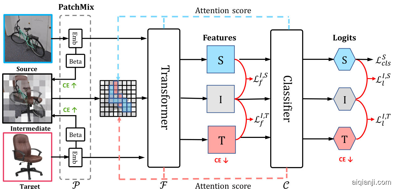
Figure 3. Overview of the proposed PMTrans framework. It consists of three players: the PatchMix module empowered by a patch embedding mathbf{(Emb)} layer and a learnable Beta distribution (Beta), ViT encoder, and classifier.
图 3: 提出的 PMTrans 框架概览。它包含三个部分:由补丁嵌入层 (Emb) 和可学习的 Beta 分布 (Beta) 驱动的 PatchMix 模块、ViT 编码器和分类器。
where alpha is the trade-off parameter, ell is the supervised classification loss for the source domain, and mathbf{CE}_{s,i,t}(omega) is the discrepancy between the intermediate domain and the source/target domain. The definitions of mathcal{L}_{c l s}^{S}(omega_{mathcal{F}},omega_{mathcal{C}}) and mathbf{CE}_{s,i,t}(omega) are shown in Sec. 3.2. As illustrated in Eq. 4, the game is essentially a min-max process, i.e., a competition for the player mathcal{P} against both players mathcal{F} and mathcal{C} . Specifically, as depicted in Fig. 3, mathcal{P} strives to diverge while mathcal{F} and mathcal{C} try to align domain distributions, which is a min-max process on CE. In this min-max CE game, each player behaves selfishly to reduce its cost function, and this competition will possibly end with a situation where no one has anything to gain by changing only one’s strategy. This situation is called Nash Equilibrium (NE) in game theory.
其中 alpha 是权衡参数,ell 是源域的监督分类损失,mathbf{CE}_{s,i,t}(omega) 是中间域与源/目标域之间的差异。mathcal{L}_{c l s}^{S}(omega_{mathcal{F}},omega_{mathcal{C}}) 和 mathbf{CE}_{s,i,t}(omega) 的定义如第3.2节所示。如公式4所示,该博弈本质上是一个极小极大过程,即玩家 mathcal{P} 与玩家 mathcal{F} 和 mathcal{C} 之间的竞争。具体而言,如图3所示,mathcal{P} 努力使分布发散,而 mathcal{F} 和 mathcal{C} 则试图对齐域分布,这是关于CE的极小极大过程。在这个极小极大CE博弈中,每个玩家都自私地试图降低其成本函数,这种竞争可能会以这样一种情况结束:即没有人可以通过仅改变自己的策略而获得任何收益。这种情况在博弈论中被称为纳什均衡 (Nash Equilibrium, NE)。
Definition 2 (Nash Equilibrium): The equilibrium states each player’s strategy is the best response to other players. And a point omega^ {*}inOmega is Nash Equilibrium i f
定义 2 (纳什均衡): 均衡状态下每个参与者的策略都是对其他参与者策略的最佳回应。若点 omega^{*}inOmega 满足该条件,则称为纳什均衡 (Nash Equilibrium) 。
Intuitively, in our case, NE means that no player has the incentive to change its own parameters, as there is no additional pay-off.
直观来看,在我们的案例中,纳什均衡(NE)意味着任何玩家都没有动机改变自身参数,因为无法获得额外收益。
3.2. The Proposed Framework
3.2. 提出的框架
Overview. Fig. 3 illustrates the framework of our proposed PMTrans, which consists of a ViT encoder, a classifier, and a PatchMix module. PatchMix module is utilized to maximize the CE between the intermediate domain and source/target domain, conversely, two semi-supervised mixup losses in the feature and label spaces are proposed to minimize CE. Finally, a three-player game containing feature extractor, classifier, and PatchMix module, minimizes and maximizes the CE for aligning distributions between the source and target domains.
概述。图3展示了我们提出的PMTrans框架,该框架由ViT编码器、分类器和PatchMix模块组成。PatchMix模块用于最大化中间域与源/目标域之间的交叉熵(CE),相反,我们提出了特征空间和标签空间中的两种半监督混合损失以最小化CE。最终,包含特征提取器、分类器和PatchMix模块的三方博弈通过最小化和最大化CE来实现源域与目标域的分布对齐。
PatchMix. As shown in Fig. 3, the PatchMix module is proposed to construct the intermediate domain, buttressed by Definition. 1. In detail, the patch embedding layer in PatchMix transforms input images from source/target domains into patches. And the ViT encoder aims to extract features from the patch sequences. The classifier maps the outputs of ViT encoder to make predictions, each of which is exploited to select the feature map to re-weight the patch sequences. The PatchMix with a learnable Beta distribution aims to maximize the CE between the intermediate and source/target domain, and is presented as follows.
PatchMix。如图 3 所示,PatchMix 模块基于定义 1 构建中间域。具体而言,PatchMix 中的 patch embedding 层将源/目标域的输入图像转换为 patch。ViT 编码器负责从 patch 序列中提取特征。分类器将 ViT 编码器的输出映射为预测结果,每个预测结果用于选择特征图来重新加权 patch 序列。具有可学习 Beta 分布的 PatchMix 旨在最大化中间域与源/目标域之间的交叉熵 (CE) ,其实现如下。
When exploiting PatchMix to construct the intermediate domain, it is worth noting that not all patches have equal contributions for the label assignment. As Chen et al. [5] observed, the mixed image has no valid objects due to the random process while there is still a response in the label space. To remedy this issue, we re-weight mathcal{P}_{lambda}({pmb y}^{s},{pmb y}^{t}) in Definition. 1 with the normalized attention score a_{k} . For the implementation details of attention scores, refer to the suppl. material. The re-scaled mathcal{P}_{lambda}({pmb y}^{s},{pmb y}^{t}) is defined as
在利用PatchMix构建中间域时,值得注意的是并非所有图像块对标签分配的贡献均等。如Chen等人[5]所观察到的,由于随机混合过程可能导致合成图像不包含有效物体,但标签空间仍会产生响应。为解决此问题,我们通过归一化注意力分数a_{k}对定义1中的mathcal{P}_{lambda}({pmb y}^{s},{pmb y}^{t})进行重新加权。注意力分数的具体实现细节可参考补充材料。重新调整后的mathcal{P}_{lambda}({pmb y}^{s},{pmb y}^{t})定义为
where
哪里
Semi-supervised mixup loss. As PatchMix tries to maximize the CE between the intermediate domain and source/target domain, we now need to find a way to minimize the CE in the game. Intuitively, we propose two semi-supervised mixup losses in the feature and label spaces to minimize the discrepancy between features of mixing patches and corresponding mixing labels based on Theorem. 1. The objective of the proposed PMTrans is show in Fig. 4 (a) and consists of a classification loss of source data and two semi-supervised mixup losses.
半监督混合损失。由于PatchMix试图最大化中间域与源/目标域之间的交叉熵(CE),我们现在需要找到一种在博弈中最小化CE的方法。直观上,我们基于定理1在特征空间和标签空间提出了两种半监督混合损失,以最小化混合图像块特征与对应混合标签之间的差异。如图4(a)所示,PMTrans的目标由源数据分类损失和两个半监督混合损失组成。
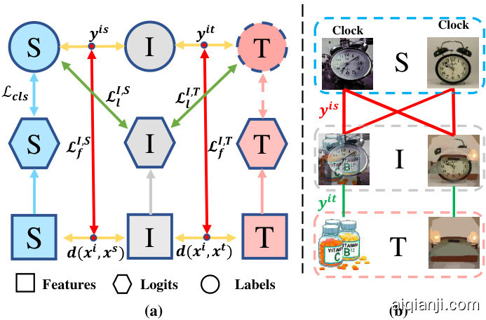
Figure 4. (a) The illustration of two proposed semi-supervised losses. (b) Label similarity {pmb y}^{i s} and {pmb y}^{i t} . Better viewed in color.
图 4: (a) 两种提出的半监督损失示意图。(b) 标签相似度 {pmb y}^{i s} 和 {pmb y}^{i t}。建议彩色查看。
- Label space: As introduced in Theorem. 1, we apply a supervised mixup loss in the label space to measure the domain divergence based on the CE loss between the mixing logits and corresponding mixing labels (See green arrow in Fig. 4 (a)).
- 标签空间:如定理1所述,我们在标签空间应用监督混合损失(supervised mixup loss),基于混合逻辑(mixing logits)与对应混合标签(mixing labels)之间的交叉熵损失(CE loss)来度量域差异(参见图4(a)中绿色箭头)。
where hat{y^{t}} is the pseudo label for target data. For convenience, we utilize the method, commonly used in [21, 22], to generate pseudo labels hat{y^{t}} for samples via k -means cluster.
其中 hat{y^{t}} 是目标数据的伪标签。为方便起见,我们采用[21, 22]中常用的方法,通过 k-means聚类为样本生成伪标签 hat{y^{t}}。
- Feature space: Nonetheless, the supervised loss alone in the label space is not sufficient to diminish the domain divergence due to the less reliable pseudo labels of the target data. Therefore, we further propose to minimize the discrepancy between the similarity of the features and the similarity of labels in the feature space for aligning the intermediate and source/target domain without the supervised information of the target domain. The experimental results in Tab. 5 validate its effectiveness.
- 特征空间 (Feature space): 然而,仅靠标签空间中的监督损失不足以减小域差异,因为目标数据的伪标签可靠性较低。为此,我们进一步提出在特征空间中最小化特征相似性与标签相似性之间的差异,从而在没有目标域监督信息的情况下对齐中间域和源/目标域。表 5 中的实验结果验证了该方法的有效性。
Specifically, we first compute the cosine similarity between the intermediate domain and source/target domain in the feature space. The feature similarity is defined as
具体来说,我们首先计算特征空间中中间域与源域/目标域之间的余弦相似度。特征相似度定义为
where cos denotes the cosine similarity. As shown in Fig. 4(b), for the source domain, we exploit the ground-truth to calculate the label similarity, y^{i s}=bar{y^{s}}(y^{s})^{mathsf{T}} , as a binary matrix to represent whether samples share the same labels. For example, the intermediate image is constructed by sampling patches from the source image, e.g., clock; therefore, the label similarity is set as 1 if it is calculated between the intermediate image and the source class ‘clock’, otherwise, it is set as 0. Then, we utilize the CE to measure the domain discrepancy based on the difference between the feature similarity and label similarity. The supervised mixup loss in the feature space (See red arrow in Fig. 4 (a)) is formulated as
其中cos表示余弦相似度。如图4(b)所示,对于源域,我们利用真实标签计算标签相似度y^{i s}=bar{y^{s}}(y^{s})^{mathsf{T}},将其作为二元矩阵来表示样本是否共享相同标签。例如,中间图像是通过从源图像(如时钟)中采样 patches 构建的,因此当中间图像与源类别"时钟"之间计算标签相似度时设为1,否则设为0。接着,我们利用交叉熵(CE)基于特征相似度与标签相似度的差异来度量域差异。特征空间中的监督混合损失(见图4(a)红色箭头)可表示为
Moreover, for the intermediate and target domains, due to lack of supervision, we utilize identity matrix y^{i t} as the label similarity. For example, in Fig. 4 (b), as the intermediate image is built by sampling patches from the target image, e.g., bottle; therefore, the label similarity between the intermediate image and the corresponding target image is set as 1 and vice versa. To measure the divergence between the intermediate and target domains in the feature space, we propose an unsupervised mixup loss as
此外,对于中间域和目标域,由于缺乏监督,我们使用单位矩阵 y^{i t} 作为标签相似度。例如,在图4 (b) 中,由于中间图像是通过从目标图像(如瓶子)中采样补丁构建的,因此中间图像与对应目标图像之间的标签相似度设为1,反之亦然。为了衡量中间域与目标域在特征空间中的差异,我们提出了一种无监督混合损失作为
Finally, the two semi-supervised mixup losses in the feature and label spaces are formulated as
最后,特征空间和标签空间的两个半监督混合损失 (mixup) 被表述为
Moreover, the classification loss is applied to the labeled source domain data (See blue arrow in Fig. 4 (a)) and is formulated as
此外,分类损失应用于带标签的源域数据(见图4(a)中的蓝色箭头),其公式为
A Three-Player Game. Finally, the min-max CE game aims to align distributions in the feature and label spaces. The total CE between the intermediate domain and source/target domain is
三方博弈。最终,最小-最大条件熵 (CE) 博弈旨在对齐特征空间和标签空间的分布。中间域与源域/目标域之间的总条件熵为
We adopt the random mixup-ratio from a learnable Beta distribution in our PatchMix module to maximize the CE between the intermediate domain and source/target domain. Moreover, the feature extractor and classifier have the same objective to minimize the CE between the intermediate domain and source/target domain. Therefore, the total objective of PMTrans is achieved by reformulating Eq. 4 as
我们在PatchMix模块中采用可学习的Beta分布随机混合比,以最大化中间域与源/目标域之间的交叉熵(CE)。此外,特征提取器和分类器具有相同目标,即最小化中间域与源/目标域之间的交叉熵。因此,PMTrans的总目标通过将公式4重构为
where alpha is trade-off parameter. After optimizing the objective, the PatchMix module with the ideal Beta distribution will not maximize the CE anymore. Meanwhile, the feature extractor and classifier have no incentive to change their parameters to minimize the CE. Finally, the discrepancy between the intermediate domain and source/target domain is nearly zero, further indicating that the source and target domains are well aligned.
其中 alpha 是权衡参数。优化目标后,具有理想Beta分布的PatchMix模块将不再最大化交叉熵(CE)。同时,特征提取器和分类器没有动力改变其参数来最小化交叉熵。最终,中间域与源域/目标域之间的差异接近于零,进一步表明源域和目标域已良好对齐。
Table 1. Comparison with SoTA methods on Office-Home. The best performance is marked as bold.
| 方法 | A→C | A→P | A→R | C→A | C→P | C→R | P→A | P→C | P→R | R→A | R→C | R→P | 平均 | |
|---|---|---|---|---|---|---|---|---|---|---|---|---|---|---|
| ResNet-50 | 44.9 | 66.3 | 74.3 | 51.8 | 61.9 | 63.6 | 52.4 | 39.1 | 71.2 | 63.8 | 45.9 | 77.2 | 59.4 | |
| MCD | 48.9 | 68.3 | 74.6 | 61.3 | 67.6 | 68.8 | 57.0 | 47.1 | 75.1 | 69.1 | 52.2 | 79.6 | 64.1 | |
| MDD | ResNet | 54.9 | 73.7 | 77.8 | 60.0 | 71.4 | 71.8 | 61.2 | 53.6 | 78.1 | 72.5 | 60.2 | 82.3 | 68.1 |
| BNM | 56.7 | 77.5 | 81.0 | 67.3 | 76.3 | 77.1 | 65.3 | 55.1 | 82.0 | 73.6 | 57.0 | 84.3 | 71.1 | |
| FixBi | 58.1 | 77.3 | 80.4 | 67.7 | 79.5 | 78.1 | 65.8 | 57.9 | 81.7 | 76.4 | 62.9 | 86.7 | 72.7 | |
| TVT | 74.9 | 86.8 | 89.5 | 82.8 | 88.0 | 88.3 | 79.8 | 71.9 | 90.1 | 85.5 | 74.6 | 90.6 | 83.6 | |
| Deit-based | 61.8 | 79.5 | 84.3 | 75.4 | 78.8 | 81.2 | 72.8 | 55.7 | 84.4 | 78.3 | 59.3 | 86.0 | 74.8 | |
| CDTrans-Deit | ViT | 68.8 | 85.0 | 86.9 | 81.5 | 87.1 | 87.3 | 79.6 | 63.3 | 88.2 | 82.0 | 66.0 | 90.6 | 80.5 |
| PMTrans-Deit | 71.8 | 87.3 | 88.3 | 83.0 | 87.7 | 87.8 | 78.5 | 67.4 | 89.3 | 81.7 | 70.7 | 92.0 | 82.1 | |
| ViT-based | 67.0 | 85.7 | 88.1 | 80.1 | 84.1 | 86.7 | 79.5 | 67.0 | 89.4 | 83.6 | 70.2 | 91.2 | 81.1 | |
| SSRT-ViT | 75.2 | 89.0 | 91.1 | 85.1 | 88.3 | 89.9 | 85.0 | 74.2 | 91.2 | 85.7 | 78.6 | 91.8 | 85.4 | |
| PMTrans-ViT | 81.2 | 91.6 | 92.4 | 88.9 | 91.6 | 93.0 | 88.5 | 80.0 | 93.4 | 89.5 | 82.4 | 94.5 | 88.9 | |
| Swin-based | Swin | 72.7 | 87.1 | 90.6 | 84.3 | 87.3 | 89.3 | 80.6 | 68.6 | 90.3 | 84.8 | 69.4 | 91.3 | 83.6 |
| PMTrans-Swin | 81.3 | 92.9 | 92.8 | 88.4 | 93.4 | 93.2 | 87.9 | 80.4 | 93.0 | 89.0 | 80.9 | 94.8 | 89.0 |
表 1: Office-Home数据集上与当前最优方法的对比。最佳性能以粗体标注。
Table 2. Comparison with SoTA methods on Office-31. The best performance is marked as bold.
| 方法 | A→W D→W | W→D | A→ D | D→A | W→A | 平均 | |
|---|---|---|---|---|---|---|---|
| ResNet-50 BNM MDD | Net Resl | 68.9 68.4 91.5 98.5 94.5 | 62.5 100.0 100.0 | 96.7 90.3 | 60.7 70.9 | 99.3 71.6 | 76.1 87.1 |
| SCDA FixBi | 94.2 96.1 | 98.4 98.7 99.8 | 93.5 95.2 | 74.6 75.7 78.7 | 72.2 76.2 79.4 | 88.9 90.0 | |
| TVT | 99.3 96.4 99.4 | 100.0 | 95.0 96.4 | 84.9 | 86.0 | 91.4 93.9 | |
| Deit-based | 89.2 98.9 | 100.0 100.0 | 88.7 | ||||
| CDTrans-Deit | 96.7 | 99.0 | 100.0 | 80.1 | 79.8 | 89.5 | |
| PMTrans-Deit | ViT 99.0 | 99.4 | 100.0 | 97.0 | 81.1 | 81.9 | 92.6 |
| ViT-based | 91.2 | 99.2 | 96.5 | 81.4 | 82.1 | 93.1 | |
| SSRT-ViT | 97.7 | 99.2 | 100.0 | 90.4 | 81.1 | 80.6 | 91.1 |
| 100.0 | 98.6 | 83.5 | 82.2 | 93.5 | |||
| PMTrans-ViT | 99.1 99.6 | 100.0 | 99.4 | 85.7 | 86.3 | 95.0 | |
| Swin-based | Swin | 97.0 99.2 | 100.0 | 95.8 | 82.4 | 81.8 | 92.7 |
| PMTrans-Swin | 99.5 99.4 | 100.0 | 99.8 | 86.7 | 86.5 | 95.3 |
表 2. Office-31数据集上的SoTA方法对比。最佳性能以粗体标注。
4. Experiments
4. 实验
4.1. Datasets and implementation
4.1. 数据集与实现
Datasets. To evaluate the proposed method, we conduct experiments on four popular UDA benchmarks, including Office-Home [41], Office-31 [34], VisDA-2017 [33], and DomainNet [32]. The details of the datasets and transfer tasks on these datasets can be found in the suppl. material. Implementation. In all experiments, we use the Swin-based transformer [25] pre-trained on ImageNet [10] as the backbone for our PMTrans. The base learning rate is 5e^{-6} with a batch size of 32, and we train models by 50 epochs. For VisDA-2017, we use a lower learning rate 1e^{-6} . We adopt AdamW [28] with a momentum of 0.9, and a weight decay of 0.05 as the optimizer. Furthermore, for fine-tuning purposes, we set the classifier (MLP) with a higher learning rate 1e^{-5} for our main tasks and learn the trade-off parameter adaptively. For a fair comparison with prior works, we also conduct experiments with the same backbone Deit-based [38] as CDTrans [46], and ViT-based [12] as SSRT [37] on Office31, Office-Home, and VisDA-2017. These two studies are trained for 60 and 100 epochs separately.
数据集。为评估所提方法,我们在四个流行的无监督域适应(UDA)基准测试上进行实验,包括Office-Home [41]、Office-31 [34]、VisDA-2017 [33]和DomainNet [32]。数据集详情及迁移任务说明详见补充材料。
实现细节。所有实验中,我们采用基于Swin的Transformer [25]作为PMTrans主干网络,其预训练权重来自ImageNet [10]。基础学习率设为$5e^{-6},批量大小为32,训练50个周期。针对VisDA-2017数据集采用更低学习率1e^{-6}。优化器选用AdamW [28],动量0.9,权重衰减0.05。为微调分类器(MLP),主任务学习率设为1e^{-5}$并自适应学习权衡参数。
为公平对比前人工作,我们同样采用CDTrans [46]使用的Deit-based [38]主干和SSRT [37]采用的ViT-based [12]主干,在Office31、Office-Home和VisDA-2017上进行实验,这两个对照实验分别训练60和100个周期。
4.2. Results
4.2. 结果
We compare PMTrans with the SoTA methods, including ResNet-based and ViT-based methods. The ResNet-based methods are FixBi [30], MCD [35], SWD [16], SCDA [20], BNM [8], and MDD [52]. The ViT-based methods are SSRT [37], CDTrans [46], and TVT [47].
我们对比了PMTrans与当前最优方法(SoTA),包括基于ResNet和基于ViT的方法。基于ResNet的方法有FixBi [30]、MCD [35]、SWD [16]、SCDA [20]、BNM [8]和MDD [52]。基于ViT的方法包括SSRT [37]、CDTrans [46]和TVT [47]。
For the ResNet-based methods, we utilize ResNet-50 as the backbone for the Office-Home, Office-31, and DomainNet datasets, and we adopt ResNet-101 for VisDA-2017 dataset. Note that each backbone is trained with the source data only and then tested with the target data.
对于基于ResNet的方法,我们在Office-Home、Office-31和DomainNet数据集上采用ResNet-50作为主干网络,而在VisDA-2017数据集上使用ResNet-101。需要注意的是,每个主干网络仅使用源数据进行训练,然后在目标数据上进行测试。
Results on Office-Home. Tab. 1 shows the quantitative results of methods using different backbones. As expected, our PMTrans framework achieves noticeable performance gains and surpasses TVT, SSRT, and CDTrans by a large margin. Importantly, our PMTrans achieves an improvement more than 5.4% accuracy over the Swin backbone and yields 89.0% accuracy. Interestingly, our proposed PMTrans can decrease the domain divergence effectively with Deitbased and ViT-based backbones. The results indicate that our method can obtain more robust transferable representations than the CNN-based and ViT-based methods.
Office-Home数据集上的结果。表1展示了使用不同主干网络的方法量化结果。如预期所示,我们的PMTrans框架实现了显著性能提升,大幅超越TVT、SSRT和CDTrans方法。值得注意的是,PMTrans在Swin主干网络上实现了超过5.4%的准确率提升,最终达到89.0%的准确率。有趣的是,我们提出的PMTrans能有效降低基于Deit和ViT主干网络的域差异。结果表明,相比基于CNN和ViT的方法,我们的方法能获得更具鲁棒性的可迁移表征。
Results on Office-31. Tab. 2 shows the quantitative comparison with the CNN-based and ViT-based methods. Overall, our PMTrans achieves the best performance on each task with $95.3% accuracy and outperforms the SoTA methods with identical backbones. Numerically, PMTrans noticeably surpasses the SoTA methods with an increase of +1.4% accuracy over TVT, +2.7% accuracy over CDTrans, and +1.8% accuracy over SSRT, respectively.
Office-31上的结果。表2展示了与基于CNN和基于ViT方法的定量比较。总体而言,我们的PMTrans在每项任务上都取得了最佳性能,准确率达到95.3%,并在相同骨干网络下超越了SoTA方法。具体数值上,PMTrans显著优于SoTA方法:比TVT提升+1.4%准确率,比CDTrans提升+2.7%准确率,比SSRT提升+1.8%准确率。
Results on VisDA-2017. As shown in Tab. 3, our PMTrans achieves 88.0% accuracy and outperforms the baseline by 11.2% . In particular, for the ‘hard’ categories, such as ”person”, our method consistently achieves a much higher performance boost from 29.0% to 70.3% . These improvements indicate that our method shows an excellent generalization capability and achieves comparable performance mathbf88.0%)
VisDA-2017实验结果。如表3所示,我们的PMTrans实现了88.0%准确率,以11.2%的优势超越基线方法。特别是在"人物"等困难类别上,我们的方法将性能从29.0%显著提升至70.3%。这些改进表明我们的方法展现出优异的泛化能力,并取得了可比性能(88.0%)。
Table 3. Comparison with SoTA methods on VisDA-2017. The best performance is marked as bold.
表 3: VisDA-2017数据集上与SoTA方法的对比。最佳性能以粗体标出。
| 方法 | 飞机 | 自行车 | 巴士 | 汽车 | 马 | 刀具 | 摩托车 | 行人 | 植物 | 滑板 | 火车 | 卡车 | 平均 | |
|---|---|---|---|---|---|---|---|---|---|---|---|---|---|---|
| ResNet-50 | ResNet | 55.1 | 53.3 | 61.9 | 59.1 | 80.6 | 17.9 | 79.7 | 31.2 | 81.0 | 26.5 | 73.5 | 8.5 | 52.4 |
| BNM | 89.6 | 61.5 | 76.9 | 55.0 | 89.3 | 69.1 | 81.3 | 65.5 | 90.0 | 47.3 | 89.1 | 30.1 | 70.4 | |
| MCD | 87.0 | 60.9 | 83.7 | 64.0 | 88.9 | 79.6 | 84.7 | 76.9 | 88.6 | 40.3 | 83.0 | 25.8 | 71.9 | |
| SWD | 90.8 | 82.5 | 81.7 | 70.5 | 91.7 | 69.5 | 86.3 | 77.5 | 87.4 | 63.6 | 85.6 | 29.2 | 76.4 | |
| FixBi | 96.1 | 87.8 | 90.5 | 90.3 | 96.8 | 95.3 | 92.8 | 88.7 | 97.2 | 94.2 | 90.9 | 25.7 | 87.2 | |
| TVT | 82.9 | 85.6 | 77.5 | 60.5 | 93.6 | 98.2 | 89.4 | 76.4 | 93.6 | 92.0 | 91.7 | 55.7 | 83.1 | |
| Deit-based | ViT | 98.2 | 73.0 | 82.5 | 62.0 | 97.3 | 63.5 | 96.5 | 29.8 | 68.7 | 86.7 | 96.7 | 23.6 | 73.2 |
| CDTrans-Deit | 97.1 | 90.5 | 82.4 | 77.5 | 96.6 | 96.1 | 93.6 | 88.6 | 97.9 | 86.9 | 90.3 | 62.8 | 88.4 | |
| PMTrans-Deit | 98.2 | 92.2 | 88.1 | 77.0 | 97.4 | 95.8 | 94.0 | 72.1 | 97.1 | 95.2 | 94.6 | 51.0 | 87.7 | |
| ViT-based | 99.1 | 60.7 | 70.1 | 82.7 | 96.5 | 73.1 | 97.1 | 19.7 | 64.5 | 94.7 | 97.2 | 15.4 | 72.6 | |
| SSRT-ViT | 98.9 | 87.6 | 89.1 | 84.8 | 98.3 | 98.7 | 96.3 | 81.1 | 94.8 | 97.9 | 94.5 | 43.1 | 88.8 | |
| PMTrans-ViT | Swin | 98.9 | 93.7 | 84.5 | 73.3 | 99.0 | 98.0 | 96.2 | 67.8 | 94.2 | 98.4 | 96.6 | 49.0 | 87.5 |
| PMTrans-Swin | S | 99.4 | 88.3 | 88.1 | 78.9 | 98.8 | 98.3 | 95.8 | 70.3 | 94.6 | 98.3 | 96.3 | 48.5 | 88.0 |
Table 4. Comparison with SoTA methods on DomainNet. The best performance is marked as bold.
表 4: DomainNet上与SoTA方法的对比。最佳性能以粗体标出。
with the SoTA methods (mathbf88.7%}) ). PMTrans also surpasses the SoTA methods on several sub-categories, such as ”horse” and ”sktbrd”. In particular, it is shown that the SoTA methods, e.g., CDTrans and SSRT, achieve better results on this dataset. The reason is that CDTrans and SSRT are trained with a batch size of 64 while PMTrans’s batch size is 32. It indicates that when the input size is much bigger, the input can represent the data distributions better. A detailed ablation study for this issue can be found in the suppl. material.. Results on DomainNet. PMTrans achieves a very high average accuracy on the most challenging DomainNet dataset, as shown in Tab. 4. Overall, our proposed PMTrans outperforms the SoTA methods by +7.2% accuracy. Incredibly, PMTrans surpasses the SoTA methods in all the 30 subtasks, which demonstrates the strong ability of PMTrans to alleviate the large domain gap. Moreover, transferring knowledge is much more difficult when the domain gap becomes significant. When taking more challenging qdr as the target domain while others as the source domain, our
与现有最佳方法 (SoTA) 相比 (88.7%) ),PMTrans 在多个子类别(如"马"和"滑板")上也超越了 SoTA 方法。值得注意的是,CDTrans 和 SSRT 等 SoTA 方法在该数据集上表现更优,原因是它们采用 64 的批处理规模进行训练,而 PMTrans 的批处理规模为 32。这表明当输入规模更大时,输入能更好地表征数据分布。该问题的详细消融研究见补充材料。
DomainNet 数据集上的结果表明,如表 4 所示,PMTrans 在这个最具挑战性的数据集上取得了极高的平均准确率。总体而言,我们提出的 PMTrans 以 +7.2% 的准确率优势超越 SoTA 方法。令人惊叹的是,PMTrans 在所有 30 个子任务中都超越了 SoTA 方法,这证明了其在缓解大域差距方面的强大能力。此外,当域差距显著增大时,知识迁移会变得更为困难。当选择更具挑战性的 qdr 作为目标域而其他域作为源域时,我们的...
PMTrans achieves an average accuracy of $27.0% , while ViTbased SSRT and CDTrans only achieve an average accuracy of 13.7% and 1% , respectively. The comparisons on DomainNet dataset demonstrate that our PMTrans yields the best generalization ability for the challenging UDA problem.
PMTrans的平均准确率达到27.0%,而基于ViT的SSRT和CDTrans分别仅达到13.7%和1%。DomainNet数据集上的对比实验表明,我们的PMTrans在具有挑战性的无监督域适应(UDA)问题上展现出最佳的泛化能力。
4.3. Ablation Study
4.3. 消融研究
Semi-supervised mixup loss. As shown in Tab. 5, Swin with the semi-supervised mixup loss in the feature and label spaces outperforms the counterpart built on Swin with only source training by +1.0% and +4.3% on Office-Home dataset, respectively. The results indicate the effectiveness of the semi-supervised mixup loss for diminishing the domain discrepancy. Moreover, we observe that the CE loss yields better performance on the label space than that on the feature space. The reason is that the CE loss on the label space utilizing the class information performs better than on the feature space without the class information.
半监督混合损失 (semi-supervised mixup loss)。如表 5 所示,在 Office-Home 数据集上,采用特征空间和标签空间半监督混合损失的 Swin 模型,性能分别比仅使用源数据训练的 Swin 模型高出 +1.0% 和 +4.3%。结果表明,半监督混合损失能有效减小域差异。此外,我们观察到交叉熵损失 (CE loss) 在标签空间的表现优于特征空间,原因是标签空间的交叉熵损失利用了类别信息,其效果优于不包含类别信息的特征空间。
Learning hyper parameters of mixup. Tab. 6 shows the ablation results for the effects of learning hyper parameters of the Beta distribution on the Office-Home. We compare the learning hyper parameters of mixup with fixed parameters, such as Beta(1,1) and Beta(2,2). The proposed method achieves +0.9% and +0.8% accuracy increment compared with that based on Beta(1,1) and Beta(2,2). The results demonstrate that learning to estimate the distribution to build up the intermediate domain facilitates domain alignment.
学习mixup的超参数。表6展示了在Office-Home数据集上学习Beta分布超参数效果的消融实验结果。我们将学习mixup超参数的方法与固定参数(如Beta(1,1)和Beta(2,2))进行对比。相比基于Beta(1,1)和Beta(2,2)的方法,所提方法分别实现了+0.9%和+0.8%的准确率提升。结果表明,通过学习估计分布来构建中间域有助于实现域对齐。
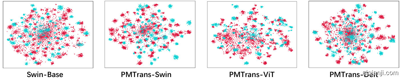
Figure 5. t-SNE visualization s for task mathrm{A}{rightarrow}mathrm{C} on the Office-Home dataset. Source and target instances are shown in blue and red, respectively.
Table 5. Effect of semi-supervised loss. The best performance is marked as bold.
图 5: Office-Home数据集上任务mathrm{A}{rightarrow}mathrm{C}的t-SNE可视化。源实例和目标实例分别用蓝色和红色表示。
| Cols | Cf | Ll | A→C | A→P | A→R | C→A | C→P | C→R | P→A | P→C | P→R | R→A | R→C | R→P | Avg | |
|---|---|---|---|---|---|---|---|---|---|---|---|---|---|---|---|---|
| 人 | 72.7 | 87.1 | 90.6 | 84.3 | 87.3 | 89.3 | 80.6 | 68.6 | 90.3 | 84.8 | 69.4 | 91.3 | 83.6 | |||
| 人 | √ | 73.9 | 87.5 | 91.0 | 85.3 | 87.9 | 89.9 | 82.8 | 72.1 | 91.2 | 86.3 | 74.1 | 92.4 | 84.6 | ||
| 人 | 79.2 | 91.8 | 92.3 | 88.0 | 92.6 | 93.0 | 87.1 | 77.8 | 92.5 | 88.2 | 78.4 | 93.9 | 87.9 | |||
| 人 | 81.3 | 92.9 | 92.8 | 88.4 | 93.4 93.2 | 87.9 | 80.4 | 93.0 | 89.0 | 80.9 | 94.8 | 89.0 |
表 5: 半监督损失的效果。最佳性能以粗体标出。
Table 6. Effect of learning parameters. The best performance is marked as bold
| 方法 | A→C | A→P | A→R | C→A | C→P | C→R | P→A | P→C | P→R | R→A | R→C | R→P | 平均 |
|---|---|---|---|---|---|---|---|---|---|---|---|---|---|
| Beta(1,1) | 79.9 | 92.0 | 92.3 | 88.6 | 92.6 | 92.4 | 86.9 | 79.0 | 92.4 | 88.2 | 79.3 | 94.0 | 88.1 |
| Beta(2,2) | 79.9 | 92.1 | 92.7 | 88.4 | 92.4 | 92.7 | 86.9 | 79.5 | 92.1 | 88.1 | 79.6 | 94.3 | 88.2 |
| Learning | 81.3 | 92.9 | 92.8 | 88.4 | 93.4 | 93.2 | 87.9 | 80.4 | 93.0 | 89.0 | 80.9 | 94.8 | 89.0 |
表 6: 学习参数的影响。最佳性能以粗体标出
Table 7. Effect of PatchMix. The best performance is marked as bold.
| 方法 | A→C | A→P | A→R | C→A | C→P | C→R | P→A | P→C | P→R | R→A | R→C | R→P | 平均 |
|---|---|---|---|---|---|---|---|---|---|---|---|---|---|
| Mixup | 79.4 | 92.4 | 92.6 | 87.5 | 92.8 | 92.4 | 86.8 | 80.3 | 92.5 | 88.2 | 79.7 | 95.4 | 88.3 |
| CutMix | 79.2 | 91.2 | 92.2 | 87.6 | 91.8 | 91.8 | 86.0 | 77.8 | 92.6 | 88.2 | 78.4 | 94.1 | 87.6 |
| PatchMix | 81.3 | 92.9 | 92.8 | 88.4 | 93.4 | 93.2 | 87.9 | 80.4 | 93.0 | 89.0 | 80.9 | 94.8 | 89.0 |
表7: PatchMix效果对比。最佳性能已加粗标注。
PatchMix. Comparisons of PMTrans with Mixup [50] and CutMix [48] are shown in Tab. 7. PMTrans outperforms Mixup and CutMix by +0.7% and +1.4% accuracy on the Office-Home dataset, demonstrating that PatchMix can capture the global and local mixture information better than the global mixture Mixup and local mixture CutMix methods.
PatchMix。PMTrans与Mixup [50]和CutMix [48]的对比结果如表7所示。在Office-Home数据集上,PMTrans的准确率分别比Mixup和CutMix高出+0.7%和+1.4%,这表明PatchMix能比全局混合的Mixup和局部混合的CutMix方法更好地捕捉全局与局部混合信息。
Visualization. In Fig. 5, we visualize the features learned by Swin-based, PMTrans-Swin, PMTrans-ViT, and PMTransDeit on task mathrm{A}tomathrm{C} from the Office-Home dataset via the t-SNE [11]. Compared with Swin-based and PMTrans-Swin, our PMTrans model can better align the two domains by constructing the intermediate domain to bridge them. Moreover, comparisons between PMTrans with different transformer backbones reveal that PMTrans works successfully with different backbones on UDA tasks. Due to the page limit, more experiments and analyses can be found in the suppl. material.
可视化。在图5中,我们通过t-SNE [11]对Office-Home数据集中任务mathrm{A}tomathrm{C}上基于Swin的模型、PMTrans-Swin、PMTrans-ViT和PMTransDeit学习到的特征进行了可视化。与基于Swin的模型和PMTrans-Swin相比,我们的PMTrans模型通过构建中间域来桥接两个域,能够更好地实现域对齐。此外,不同Transformer骨干网络的PMTrans模型比较表明,PMTrans在UDA任务中能够成功地与不同骨干网络协同工作。由于篇幅限制,更多实验和分析可参考补充材料。
5. Conclusion and Future Work
5. 结论与未来工作
In this paper, we proposed a novel method, PMTrans, an optimization solution for UDA from a game perspective. Specifically, we first proposed a novel ViT-based module called PatchMix that effectively built up the intermediate domain to learn disc rim i native domain-invariant representations for domains. And the two semi-supervised mixup losses were proposed to assist in finding the Nash Equilibria. Moreover, we leveraged attention maps from ViT to reweight the label of each patch by its significance. PMTrans achieved the SoTA results on four benchmark UDA datasets, outperforming the SoTA methods by a large margin. In the near future, we plan to implement our PatchMix and the two semi-supervised mixup losses to solve self-supervised and semi-supervised learning problems. We will also exploit our method to tackle the challenging downstream tasks, e.g., semantic segmentation and object detection.
本文提出了一种名为PMTrans的新方法,从博弈论视角优化无监督域适应(UDA)问题。具体而言,我们首先提出了基于ViT的PatchMix模块,通过构建中间域来学习具有判别性的域不变特征表示。随后设计两种半监督混合损失函数来辅助寻找纳什均衡点。此外,我们利用ViT的注意力图根据每个图像块(patch)的重要性重新加权其标签。PMTrans在四个基准UDA数据集上取得了最先进(SoTA)成果,性能显著优于现有最优方法。近期计划将PatchMix模块与两种混合损失函数应用于自监督和半监督学习问题,并将该方法拓展至语义分割、目标检测等下游任务。
tation with domain mixup. In The Thirty-Fourth AAAI Conference on Artificial Intelligence, AAAI 2020, The Thirty-Second Innovative Applications of Artificial Intelligence Conference, IAAI 2020, The Tenth AAAI Symposium on Educational Advances in Artificial Intelligence, EAAI 2020, New York, NY, USA, February 7-12, 2020, pages 6502–6509. AAAI Press, 2020. 2
在第三十四届人工智能大会 (AAAI 2020) 、第三十二届人工智能创新应用大会 (IAAI 2020) 和第十届人工智能教育进展研讨会 (EAAI 2020) 上发表的论文《领域混合的数据增强》,会议于2020年2月7日至12日在美国纽约举行,AAAI出版社出版,页码6502–6509。
olulu, Hawaii, USA, January 27 - February 1, 2019, pages 5989–5996. AAAI Press, 2019. 2 [54] Yongchun Zhu, Fuzhen Zhuang, Jindong Wang, Guolin Ke, Jingwu Chen, Jiang Bian, Hui Xiong, and Qing He. Deep subdomain adaptation network for image classification. IEEE Trans. Neural Networks Learn. Syst., 32(4):1713–1722, 2021. 1
美国夏威夷火奴鲁鲁,2019年1月27日-2月1日,第5989–5996页。AAAI出版社,2019年。2
[54] Yongchun Zhu, Fuzhen Zhuang, Jindong Wang, Guolin Ke, Jingwu Chen, Jiang Bian, Hui Xiong, Qing He. 深度子域自适应网络在图像分类中的应用。IEEE Trans. Neural Networks Learn. Syst., 32(4):1713–1722, 2021年。1
Conference, IAAI 2019, The Ninth AAAI Symposium on Educational Advances in Artificial Intelligence, EAAI 2019, Hon
会议,IAAI 2019,第九届AAAI人工智能教育进展研讨会,EAAI 2019
Patch-Mix Transformer for Unsupervised Domain Adaptation: A Game Perspective –Appendix–
基于博弈视角的无监督域自适应Patch-Mix Transformer –附录–
Jinjing Zhu1* Haotian Bai1* Lin Wang1,2† 1 AI Thrust, HKUST(GZ) 2 Dept. of CSE, HKUST zhujinjing.hkust@gmail.com, hao tian white@outlook.com, linwang@ust.hk
朱金晶1* 白昊天1* 王林1,2† 1 香港科技大学(广州)人工智能学域 2 香港科技大学计算机科学与工程系 zhujinjing.hkust@gmail.com, haotianwhite@outlook.com, linwang@ust.hk
Abstract
摘要
In this supplementary material, we first prove theorem 1 in Section 1. Then, Section 2 introduces the details of the proposed method, and Section 3 shows the algorithm of the proposed PMTrans. Section 4 and Section 5 show the results, analyses, and ablation experiments to prove the effectiveness of the proposed PMTrans. Finally, Section 6 shows some discussions and details about our proposed work.
在本补充材料中,我们首先在第1节证明定理1。接着,第2节介绍所提方法的细节,第3节展示提出的PMTrans算法。第4节和第5节通过结果、分析和消融实验证明PMTrans的有效性。最后,第6节针对所提工作展开讨论并补充细节。
1. Proof
1. 证明
1.1. Domain Distribution Estimation with PatchMix
1.1. 基于PatchMix的域分布估计
Let mathcal{H} denote the representation spaces with dimensionality mathrm{dim}({mathcal{H}}) , mathcal{F} denote the set of encoding functions i.e., the feature extractor and mathcal{C} be the set of decoding functions i.e. the classifier. Let mathcal{P}_{lambda} be the set of functions to generate mixup ratio for building the intermediate domain. Furthermore, let P_{S},P_{T} , and P_{I} be the empirical distributions of data mathcal{D}_{s} , mathcal{D}_{t} , and mathcal{D}_{i} . Define f^{star}inmathcal{F},c^{star}inmathcal{C} , and {mathcal{P}}_{lambda}^{star}in{mathcal{P}}_{lambda} be the minimizers of Eq. 1 and D(P_{S},P_{T}) as the measure of the domain divergence between P_{S} and P_{T} :
设 mathcal{H} 表示维度为 mathrm{dim}({mathcal{H}}) 的表示空间,mathcal{F} 表示编码函数集(即特征提取器),mathcal{C} 表示解码函数集(即分类器)。设 mathcal{P}_{lambda} 为生成混合比例以构建中间域的函数集。此外,令 P_{S}、P_{T} 和 P_{I} 分别为数据 mathcal{D}_{s}、mathcal{D}_{t} 和 mathcal{D}_{i} 的经验分布。定义 f^{star}inmathcal{F}、c^{star}inmathcal{C} 和 {mathcal{P}}_{lambda}^{star}in{mathcal{P}}_{lambda} 为式1的最小化解,D(P_{S},P_{T}) 为 P_{S} 与 P_{T} 之间的域差异度量:
where ell is the CE loss. Then, we can reformulate Eq.1 as:
其中 ell 是交叉熵损失 (CE loss)。于是,我们可以将公式1重新表述为:
where h_{i}^{s}=f(pmb{x}_{i}^{s}) and h_{j}^{t}=f(pmb{x}_{j}^{t}) . Inspired and borrowed by this work [23], we give proof as follows.
其中 h_{i}^{s}=f(pmb{x}_{i}^{s}) 和 h_{j}^{t}=f(pmb{x}_{j}^{t}) 。受该工作 [23] 启发并借鉴其方法,我们给出如下证明。
Theorem 1 :Let dinmathbb{N} to represent the number of classes contained in three sets mathcal{D}_{s},mathcal{D}_{t} , and mathcal{D}_{i} . If cdotmathrm{dim}({mathcal{H}})geq d-1 , mathcal{P}_{lambda}{'}ellbig(c^{star}big(f^{star}(x_{i})big),y^{s}big)+(1-mathcal{P}_{lambda}{'})ellbig(c^{star}big(f^{star}(x_{i})big),y^{t}big)=0, , then Dleft(P_{S},P_{T}right)=0 and the corresponding minimizer c^{star} is a linear function from mathcal{H} to mathbb{R}^{d} . Denote the scaled mixup ratio sampled from a learnable Beta distribution as mathcal{P}_{lambda}^{prime} .
定理1: 设dinmathbb{N}表示三个集合mathcal{D}_{s},mathcal{D}_{t}和mathcal{D}_{i}中包含的类别数。若cdotmathrm{dim}({mathcal{H}})geq d-1,且mathcal{P}_{lambda}{'}ellbig(c^{star}big(f^{star}(x_{i})big),y^{s}big)+(1-mathcal{P}_{lambda}{'})ellbig(c^{star}big(f^{star}(x_{i})big),y^{t}big)=0,,则Dleft(P_{S},P_{T}right)=0,且对应的最小化器c^{star}是从mathcal{H}到mathbb{R}^{d}的线性函数。将从可学习的Beta分布中采样的缩放混合比记为mathcal{P}_{lambda}^{prime}。
Proof: First, the following statement is true if mathrm{dim}(mathscr{H})geq d-1 :
证明:首先,当 mathrm{dim}(mathscr{H})geq d-1 时,以下命题成立:
where I_{dtimes d} and $1_{d} denote the d -dimensional identity matrix and all-one vector, respectively. In fact, b_{d}^{top} is a rank-one matrix, and the rank of the identity matrix is d . Since the column set span of I_{dtimes d} needs to be contained in the span of A^{top}H+b_{d}^{top} , A^{top}H only needs to be a matrix with the rank d-1$ to meet this requirement.
其中 I_{dtimes d} 和 $1_{d} 分别表示 d 维单位矩阵和全1向量。实际上,b_{d}^{top} 是一个秩为1的矩阵,而单位矩阵的秩为 d。由于 I_{dtimes d} 的列空间需要包含在 A^{top}H+b_{d}^{top} 的列空间中,A^{top}H 只需是一个秩为 d-1$ 的矩阵即可满足这一要求。
Let c^{star}(h)=A^{top}h+b , for all hin{mathcal{H}} . Let f^{star}left(pmb{x}_{i}^{s}right)= H_{zeta_{i}^{s}} ,: and f^{star}left(pmb{x}_{j}^{t}right)=H_{zeta_{j}^{t}}, ,: be the zeta_{i} -th and zeta_{j} -th slice of H , respectively. Specifically, zeta_{i}^{s},zeta_{i}^{t}in{1,dots,d} stand for the class-index of the examples pmb{x}_{i}^{s} and boldsymbol{x}_{j}^{t} . Given Eq.1, the intermediate domain sample begin{array}{r}{pmb{x}_{i j}^{i}=mathcal{P}_{lambda}^{star}(pmb{a}_{i},pmb{b}_{j})=mathcal{P}_{lambda}^{prime}cdotpmb{a}_{i}+}end{array} (1-P_{lambda}^{prime})cdot b_{j} , and the definition of cross-entropy loss ell , we get:
设 c^{star}(h)=A^{top}h+b,对于所有 hin{mathcal{H}}。令 f^{star}left(pmb{x}_{i}^{s}right)= H_{zeta_{i}^{s}},且 f^{star}left(pmb{x}_{j}^{t}right)=H_{zeta_{j}^{t}},分别为 H 的第 zeta_{i} 和第 zeta_{j} 个切片。具体而言,zeta_{i}^{s},zeta_{i}^{t}in{1,dots,d} 表示样本 pmb{x}_{i}^{s} 和 boldsymbol{x}_{j}^{t} 的类别索引。根据式(1),中间域样本 begin{array}{r}{pmb{x}_{i j}^{i}=mathcal{P}_{lambda}^{star}(pmb{a}_{i},pmb{b}_{j})=mathcal{P}_{lambda}^{prime}cdotpmb{a}_{i}+}end{array} (1-P_{lambda}^{prime})cdot b_{j},以及交叉熵损失 ell 的定义,我们得到:
Eq. 3 reveals that the source and target domains are aligned if mixing the patches from two domains is equivalent to mixing the corresponding labels.
式3表明,当混合两个域的图像块等同于混合对应标签时,源域与目标域即实现对齐。
Furthermore, we see the following:
此外,我们还发现:

Figure 1. (a) Deit/ViT attention scores with the CLS token. (b) Swin attention scores with an output unit of Classifier that refers to C_{i} . The dashed line denotes the sequence with each square representing a patch.
图 1: (a) 使用CLS token的Deit/ViT注意力分数。(b) Swin注意力分数,其输出单元为分类器 C_{i}。虚线表示由每个方块代表一个图像块的序列。
The result follows from A^{top}H_{zeta_{i}^{s},:}+b=y_{i,zeta_{i}^{s}} for all i , and A^{top}H_{zeta_{j}^{t},:}+b=y_{i,zeta_{j}^{t}} for all j . If dim({mathcal{H}})geq d-1,f^{star}left({pmb x}_{i}^{t}right) and f^{star}left(x_{j}^{t}right) in the representation space mathcal{H} have some degrees of freedom to move independently. It also implies that when Eq. 3 is minimized, the representation of each class lies on a subspace of dimension mathrm{dim}({mathcal{H}})-d+1 , and with larger d i m(mathscr{H}) , the majority of directions in mathcal{H} -space will contain zero variance in the class-conditional manifold.
结果由 A^{top}H_{zeta_{i}^{s},:}+b=y_{i,zeta_{i}^{s}} 对所有 i 成立,以及 A^{top}H_{zeta_{j}^{t},:}+b=y_{i,zeta_{j}^{t}} 对所有 j 成立推导得出。若 dim({mathcal{H}})geq d-1,则表征空间 mathcal{H} 中的 f^{star}left({pmb x}_{i}^{t}right) 和 f^{star}left(x_{j}^{t}right) 具有一定程度的独立移动自由度。这也意味着当式3最小时,每个类的表征位于维度为 mathrm{dim}({mathcal{H}})-d+1 的子空间上,且随着 dim(mathscr{H}) 增大,mathcal{H} 空间中的大多数方向在类条件流形上将呈现零方差。
In practice, we utilize Eq. 3 to measure the domain gaps between the intermediate domain, and other domains and decrease them in the label and feature space, as illustrated in the main paper.
在实践中,我们利用公式3来衡量中间域与其他域之间的领域差距,并在标签和特征空间中减小这些差距,如主论文所述。
2. Details
2. 详情
2.1. Datasets
2.1. 数据集
To evaluate the proposed method, we conduct extensive experiments on four popular UDA benchmarks, including Office-31 [17], Office-Home [22], VisDA-2017 [16], and DomainNet [15].
为评估所提方法,我们在四个主流无监督域适应(UDA)基准数据集上进行了广泛实验,包括Office-31 [17]、Office-Home [22]、VisDA-2017 [16]和DomainNet [15]。
Office-31 consists of 4110 images of 31 categories, with three domains: Amazon (A), Webcam (W), and DSLR (D).
Office-31包含31个类别的4110张图像,涵盖三个域:Amazon (A)、Webcam (W)和DSLR (D)。
Office-Home is collected from four domains: Artistic images (A), Clip Art (C), Product images (P), and RealWorld images (R) and consists of 15500 images from 65 classes.
Office-Home数据集包含四个领域:艺术图像 (A)、剪贴画 (C)、产品图像 (P) 和真实世界图像 (R),共包含65个类别的15500张图像。
VisDA-2017 is a more challenging dataset for syntheticto-real domain adaptation. We set 152397 synthetic images as the source domain data and 55388 real-world images as the target domain data.
VisDA-2017是一个更具挑战性的合成到真实域适应数据集。我们将152397张合成图像设为源域数据,55388张真实世界图像设为目标域数据。
DomainNet is a large-scale benchmark dataset, which has 345 classes from six domains (Clipart (clp), Infograph (inf), Painting (pnt), Quickdraw (qdr), Real (rel), and Sketch (skt)).
DomainNet是一个大规模基准数据集,包含来自六个领域(剪贴画(clp)、信息图(inf)、绘画(pnt)、快速绘图(qdr)、实物(rel)和草图(skt))的345个类别。
2.2. Attention Map
2.2. 注意力图 (Attention Map)
We calculate the attention score in two ways based on whether the CLS token is present in the sequence. For Swin Transformer, we adopt a method similar to CAM [31] instead of changing the backbone from CNN to Transformer. Specifically, for a given image, let f_{k}(x,y) represent the encoded patch k in the last layer at spatial location (x,y) . The output of Transformer is followed by a global average pooling (GAP) layer textstylesum(x,y) and a linear classification head. For the specific class C_{i} , the classification score S_{C_{i}} is:
我们根据序列中是否存在CLS token采用两种方式计算注意力分数。对于Swin Transformer,我们采用类似于CAM [31]的方法,而非将主干网络从CNN改为Transformer。具体而言,给定图像时,令f_{k}(x,y)表示最后一层空间位置(x,y)处编码的patch k。Transformer输出后接全局平均池化(GAP)层textstylesum(x,y)和线性分类头。对于特定类别C_{i},分类分数S_{C_{i}}为:
where w_{j}^{C_{i}} represents the weight corresponding to class C_{i} for unit j in the hidden dimension. Eq.5 ensembles the semantics over both spatial contexts textstylesum(x,y) and the linear head units textstylesum(j) . Then given Eq.5, as shown in Fig.1 (b), for a given C_{i} , we reallocate the semantic information from the output of linear head unit of C_{i} . In detail, we define the semantic activation map at location (x,y) for a specific class C_{i} as:
其中 w_{j}^{C_{i}} 表示隐藏维度中单元 j 对应类别 C_{i} 的权重。公式5整合了空间上下文 textstylesum(x,y) 和线性头部单元 textstylesum(j) 的语义信息。如图1(b)所示,对于给定类别 C_{i} ,我们重新分配来自其线性头部单元输出的语义信息。具体而言,我们将特定类别 C_{i} 在位置 (x,y) 的语义激活图定义为:
where M_{C_{i}}inmathbb{R}^{2} is the activation for class C_{i} , and we infer C_{i} by the ground-truth label in the source domain and the pseudo-label in the target domain to obtain the corresponding class activation map to build the intermediate domain. Then, we use M_{C_{i}} as the attention map after the softmax operation.
其中 M_{C_{i}}inmathbb{R}^{2} 是类别 C_{i} 的激活值,我们通过源域的真实标签和目标域的伪标签推断 C_{i},从而获取对应的类别激活图以构建中间域。随后,我们将经过softmax运算后的 M_{C_{i}} 作为注意力图。
On the other hand, when the CLS token is present in the output sequence of Transformer like Deit/ViT, we simply take the attention scores from the self-attention, i.e. the similarity matrix of each layer i in Transformer A t t n_{i}in mathcal{R}^{Htimes Ntimes N} , and take the average in the head dimension H :
另一方面,当CLS token存在于Deit/ViT等Transformer的输出序列中时,我们直接采用自注意力机制中的注意力分数,即Transformer每一层i的相似度矩阵Attn_{i}inmathcal{R}^{Htimes Ntimes N},并在头维度H上取平均值:
where N is the sequence length. Next, we only take the CLS token’s attention after the softmax operation, as shown in
其中 N 为序列长度。接下来,我们仅取经过 softmax 操作后的 CLS token 注意力权重,如

Figure 2. Illustration of the semi-supervised loss in feature space.
图 2: 特征空间中半监督损失的示意图。
Fig.1 (a), and then summarize each layer’s scores to obtain the final attention scores A t t n .
图 1: (a) 然后汇总每一层的得分以获得最终的注意力分数 Attn。
2.3. Semi-supervised mixup loss in the feature space
2.3. 特征空间中的半监督混合损失
In Fig.2, we illustrate the semi-supervised loss in the feature space by similarity between features (in Fig. 2 (a)) and label spaces(in Fig.2 (b)). To compute the similarity of features, we use the normalized cosine similarity loss between the intermediate domain (column) and source/target domain(row) in the feature space, as shown in Fig.2(a). Each row denotes the normalized similarity between a sample of the intermediate domain and counterparts from the source domains. For example, we first use the cosine similarity to calculate the similarities between one intermediate sample ”car” and four sources (or target) samples (car, clock, apple, sketch clock). Then we normalize these similarities. As for the similarity of outputs (or) labels, since the source samples are labeled, and the target samples are unlabeled, we design two different methods to calculate the supervised and unsupervised label similarities. As for the label similarity between the intermediate and source domains, the intermediate and source samples both share the same labels. Therefore, we define the label similarity {pmb y}^{i s}={pmb y}^{s}({pmb y}^{s})^{top} , as shown in Fig.2 (b). Specifically, {pmb y}^{i s} , denoted by the yellow and pink colors, indicates that the label similarity between samples is one for these samples with the same labels (zero for different labels). For example, the label similarities between one intermediate sample ”sketch clock” and four sources (or target) samples car, clock, apple, and sketch clock are zero, one, zero, and one. As for the label similarity between the intermediate and target samples, we only know that the intermediate and source samples both share overlapped patches due to lack of supervision. Therefore, the label similarity {pmb y}^{i t} between samples with overlapped patches should be one (pink color), and others should be zero. And we define the label similarity {pmb y}^{i t} as identity matrix. For example, the label similarities between one unlabeled intermediate sample ”sketch clock” and four unlabeled target samples car, real clock, apple, and sketch clock are zero, zero, zero, and one. After obtaining the feature and label similarities, we utilize the CE loss ell to measure the discrepancy between these similarities as the domain gap between the intermediate and other domains.
在图2中,我们通过特征空间中的相似性(图2(a))和标签空间(图2(b))展示了半监督损失。为了计算特征相似度,我们使用特征空间中中间域(列)与源/目标域(行)之间的归一化余弦相似度损失,如图2(a)所示。每行表示中间域样本与源域对应样本之间的归一化相似度。例如,我们首先使用余弦相似度计算中间样本"car"与四个源(或目标)样本(car, clock, apple, sketch clock)之间的相似度,然后对这些相似度进行归一化处理。
对于输出(或标签)的相似度,由于源样本带有标签而目标样本无标签,我们设计了两种不同方法来计算有监督和无监督的标签相似度。中间域与源域之间的标签相似度计算中,中间样本和源样本共享相同标签。因此,我们定义标签相似度为{pmb y}^{i s}={pmb y}^{s}({pmb y}^{s})^{top},如图2(b)所示。具体而言,用黄色和粉色表示的{pmb y}^{i s}表明相同标签样本间的相似度为1(不同标签则为0)。例如,中间样本"sketch clock"与四个源(或目标)样本car, clock, apple, sketch clock的标签相似度分别为0,1,0,1。
对于中间域与目标域样本的标签相似度,由于缺乏监督信息,我们仅知道中间样本和源样本共享重叠图像块。因此,具有重叠图像块的样本间标签相似度{pmb y}^{i t}应为1(粉色),其余为0。我们将{pmb y}^{i t}定义为单位矩阵。例如,未标注的中间样本"sketch clock"与四个未标注目标样本car, real clock, apple, sketch clock的标签相似度分别为0,0,0,1。
在获得特征和标签相似度后,我们利用CE损失ell来衡量这些相似度之间的差异,作为中间域与其他域之间的域间隙。
2.4. Optimization
2.4. 优化
In our game, m -th player is endowed with a cost function J_{m} and strives to reduce its cost, which contributes to the change of CE. We now define each player’s cost function J_{m} as
在我们的游戏中,第 m 位玩家被赋予一个成本函数 J_{m} ,并努力降低其成本,这会导致CE的变化。我们现在将每位玩家的成本函数 J_{m} 定义为
where alpha is the trade-off parameter, ell is the supervised classification loss for the source domain, and mathbf{CE}_{s,i,t}(omega) is the discrepancy between the intermediate domain and the source/target domain. To clarify the min-max process, we introduce the game’s vector field v(w) , which is identical to the gradient for every player.
其中 alpha 是权衡参数,ell 是源域的监督分类损失,mathbf{CE}_{s,i,t}(omega) 是中间域与源/目标域之间的差异。为了阐明最小-最大过程,我们引入了博弈的向量场 v(w),它与每个玩家的梯度相同。
Definition 1 (Vector field): .
定义1 (Vector field):
By examining Definition.1 with respect to Eq.(6), the process can be categorized into both cooperation and competition [1].
通过将定义1与方程(6)进行对比分析,该过程可归类为合作与竞争并存 [1]。
where the left part is related to the gradient of mathcal{L}_{c l s}^{S}(omega_{mathcal{F}},omega_{mathcal{C}}) , and the right part denotes the adversarial behavior on producing or consuming CE in the network. In this Min-max CE Game, each player behaves selfishly to reduce their cost function. This competition on the network’s CE will possibly end with a situation where no one has anything to gain by changing only one’s strategy, called NE. Note that our method does not require explicit usage of gradient reverse layers as the prior GAN-based game design [6]. Our training is optimized as
其中左侧部分与 mathcal{L}_{c l s}^{S}(omega_{mathcal{F}},omega_{mathcal{C}}) 的梯度相关,右侧表示网络中生成或消耗CE (Counterfactual Explanation) 的对抗行为。在这个最小-最大CE博弈中,每个参与者都自私地行动以降低其成本函数。这种对网络CE的竞争可能以纳什均衡 (NE) 状态结束,即任何单方面改变策略都无法获得额外收益。值得注意的是,我们的方法无需像先前基于GAN的博弈设计 [6] 那样显式使用梯度反转层。训练优化过程为
2.5. Comparisons with Mixup variants
2.5. 与Mixup变体的比较
In Fig. 3, we show the visual comparisons between the PatchMix and mainstream Mixup variants. Mixup [28] mixes two samples by interpolating both the images and labels, which suffers from the local ambiguity. CutOut [4] proposes to randomly mask out square regions of input during training to improve the robustness of the CNNs. Since CutOut decreases the ImageNet localization or object detection performances, CutMix [27] is further introduced to randomly cut and paste the regions in an image, where the ground truth labels are also mixed proportionally to the area of the regions. However, sometimes there is no valid object in the mixed image due to the random process in augmentation, but there is still a response in the label space. Therefore, not all pixels are created equal, and the labels of pixels should be re-weighted. TransMix [2] is proposed to utilize the attention map to assign the confidence for the mixed samples and re-weighted the labels of pixels. In comparison, we unify these global and local mixup techniques in our PatchMix by learning to combine two patches to form a mixed patch and obtain mixed samples. Furthermore, we also learn the hyperparameters of the mixup ratio for each patch and effectively build up the intermediate domain samples.
在图 3 中,我们展示了 PatchMix 与主流 Mixup 变体的视觉对比。Mixup [28] 通过对图像和标签进行插值来混合两个样本,但存在局部模糊性问题。CutOut [4] 提出在训练期间随机遮盖输入的正方形区域以提升 CNN (Convolutional Neural Network) 的鲁棒性。由于 CutOut 会降低 ImageNet 定位或目标检测性能,CutMix [27] 进一步引入随机裁剪并粘贴图像区域的方法,其中真实标签也按区域面积比例混合。然而,由于数据增强的随机性,混合图像有时并不包含有效物体,但标签空间仍存在响应。因此,并非所有像素都具有同等重要性,像素标签应重新加权。TransMix [2] 提出利用注意力图为混合样本分配置信度,并对像素标签进行重新加权。相比之下,我们通过让模型学习组合两个图像块 (patch) 来形成混合块并生成混合样本,从而在 PatchMix 中统一了这些全局和局部混合技术。此外,我们还学习每个图像块的混合比例超参数,有效构建了中间域样本。
3. Algorithm
3. 算法
In summary, the whole algorithm to train the proposed PMTrans is shown in Algorithm 1.
总之,训练所提出的PMTrans的完整算法如算法1所示。
Algorithm 1 Patch-Mix Transformer for Unsupervised Domain Adaptation
算法 1: 用于无监督域自适应的 Patch-Mix Transformer
Require: source domain data mathcal{D}_{s} and target domain data mathcal{D}_{t} .
要求:源域数据 mathcal{D}_{s} 和目标域数据 mathcal{D}_{t}。
where the related loss functions are shown as follows.
相关损失函数如下所示。
Note that these above equations are introduced in detail in the main paper.
请注意,上述方程在主论文中有详细介绍。
4. Results and Analyses
4. 结果与分析
4.1. The comparisons on the Office-31, OfficeHome, and VisDA-2017
4.1. Office-31、OfficeHome 和 VisDA-2017 上的比较
We compare PMTrans with the SoTA methods, including ResNet- and ViT-based methods. The ResNet-based methods are FixBi [14], CGDM [5], MCD [18], SWD [9], SCDA [11], BNM [3], MDD [29], CKB [13], TSA [10], DWL [24], ILA [19], Symnets [30], CAN [8], and PCT [21]. The ViTbased methods are SSRT [20], CDTrans [25], and TVT [26], and we directly quote the results in their original papers for fair comparison. And the more detailed comparisons on three datasets are shown as Tab. 1, Tab. 2 , and Tab. 3.
我们将PMTrans与当前最先进(SoTA)方法进行比较,包括基于ResNet和ViT的方法。基于ResNet的方法包括FixBi [14]、CGDM [5]、MCD [18]、SWD [9]、SCDA [11]、BNM [3]、MDD [29]、CKB [13]、TSA [10]、DWL [24]、ILA [19]、Symnets [30]、CAN [8]和PCT [21]。基于ViT的方法包括SSRT [20]、CDTrans [25]和TVT [26],为公平比较我们直接引用其原始论文中的结果。三个数据集的详细比较见 表1、表2 和 表3。
4.2. Training
4.2. 训练
We show the progress of training on PMTrans-Swin, PMTrans-Deit, and PMTrans-ViT. To specify how each loss changes, including semi-supervised mixup loss in the label space mathcal{L}_{l} , semi-supervised mixup loss in the feature space mathcal{L}_{f} , and source classification loss mathcal{L}_{c l s}^{S} , we conduct the experiment on task Arightarrow C on Office-Home for above architectures, and the results are shown in Fig.5. We observe that for all models, both mathcal{L}_{f} and mathcal{L}_{l} drop constantly, which means the domain gap is reducing as the training evolves. Significantly, mathcal{L}_{f} fluctuates more than mathcal{L}_{l} as it aligns the domains in the feature space with a higher dimension.
我们展示了PMTrans-Swin、PMTrans-Deit和PMTrans-ViT的训练进展。为了说明各项损失的变化情况(包括标签空间中的半监督混合损失mathcal{L}_{l}、特征空间中的半监督混合损失mathcal{L}_{f}以及源分类损失mathcal{L}_{c l s}^{S}),我们在Office-Home数据集上针对Arightarrow C任务对上述架构进行了实验,结果如图5所示。观察到所有模型的mathcal{L}_{f}和mathcal{L}_{l}均持续下降,表明随着训练进行,域间差距正在缩小。值得注意的是,由于mathcal{L}_{f}需在更高维度的特征空间中对齐域,其波动幅度大于mathcal{L}_{l}。

Figure 3. PMTrans and Mixup variants
图 3: PMTrans与Mixup变体

Figure 4. Accuracy on the task mathrm{A}tomathrm{C} (Office-Home)
图 4: 任务 mathrm{A}tomathrm{C} (Office-Home) 的准确率
Table 1. Comparison with SoTA methods on Office-31. The best performance is marked as bold.
表 1: Office-31数据集上与其他先进方法的比较。最佳性能以粗体标出。
| 方法 | A→W | D→W | W→D | A→D | D→A | W→A | 平均 | |
|---|---|---|---|---|---|---|---|---|
| ResNet-50 | ResNet | 68.9 | 68.4 | 62.5 | 96.7 | 60.7 | 99.3 | 76.1 |
| BNM | 91.5 | 98.5 | 100.0 | 90.3 | 70.9 | 71.6 | 87.1 | |
| DWL | 89.2 | 99.2 | 100.0 | 91.2 | 73.1 | 69.8 | 87.1 | |
| MDD | 94.5 | 98.4 | 100.0 | 93.5 | 74.6 | 72.2 | 88.9 | |
| TSA | 94.8 | 99.1 | 100.0 | 92.6 | 74.9 | 74.4 | 89.3 | |
| ILA+CDAN | 95.7 | 99.2 | 100.0 | 93.4 | 72.1 | 75.4 | 89.3 | |
| PCT | 94.6 | 98.7 | 99.9 | 93.8 | 77.2 | 76.0 | 90.0 | |
| SCDA FixBi | 94.2 96.1 | 98.7 99.3 | 99.8 100.0 | 95.2 | 75.7 | 76.2 | 90.0 | |
| TVT | ViT | 96.4 | 95.0 | 78.7 | 79.4 | 91.4 | ||
| Deit-Base | 89.2 | 99.4 98.9 | 100.0 | 96.4 | 84.9 | 86.0 | 93.9 | |
| CDTrans-Deit | 96.7 | 99.0 | 100.0 100.0 | 88.7 | 80.1 | 79.8 | 89.5 | |
| PMTrans-Deit | 99.0 | 99.4 | 100.0 | 97.0 | 81.1 81.4 | 81.9 82.1 | 92.6 | |
| ViT-Base | 91.2 | 99.2 | 100.0 | 96.5 | 93.1 | |||
| SSRT-ViT | 90.4 | 81.1 | 80.6 | 91.1 | ||||
| PMTrans-ViT | 97.7 99.1 | 99.2 | 100.0 | 98.6 | 83.5 | 82.2 | 93.5 | |
| Swin-Base PMTrans-Swin | Swin | 99.6 | 100.0 | 99.4 | 85.7 | 86.3 | 95.0 | |
| 97.0 99.5 | 99.2 99.4 | 100.0 100.0 | 95.8 99.8 | 82.4 86.7 | 81.8 86.5 | 92.7 95.3 |
4.3. Testing
4.3. 测试
In Fig.4, we testify PMTrans-Swin, PMTrans-ViT, and PMTrans-Deit on the task mathrm{~A~}tomathrm{~C~} on the Office-Home dataset. From Fig. 4, with the same number of epochs, PMTrans-ViT achieves faster convergence than PMTransSwin and PMTrans-Deit. Besides, the results further reveal that our proposed PMTrans with different transformer backbones can bridge the source and target domains well and decrease domain divergence effectively.
在图4中,我们在Office-Home数据集上测试了PMTrans-Swin、PMTrans-ViT和PMTrans-Deit在任务mathrm{~A~}tomathrm{~C~}上的表现。从图4可以看出,在相同训练周期下,PMTrans-ViT比PMTrans-Swin和PMTrans-Deit收敛更快。此外,结果进一步表明,我们提出的PMTrans框架搭配不同Transformer骨干网络都能有效弥合源域与目标域之间的差异,显著降低领域偏移。
4.4. Complexity
4.4. 复杂度
We compare our computational budget with the typical work CDTrans [25] on aligning the source and target domains, excluding the choice of backbone. Precisely, CDTrans compute the similarity between patches from two domains by the multi-head self-attention. We are given n as the sequence length, d as the representation dimension, and c as the number of classes. The per-layer complexity is O(n^{2}d) . While in PMTrans, we adopt CE loss to close the domain gap on both the feature and label spaces of the out, whose complexity is O(d)+O(c) . When building the intermediate domain, PatchMix samples patches element-wisely, and its complexity is O(n) . As attention scores we use are taken directly from the parameters of Transformer and Classifier, so it brings no additional cost. PMTrans’s complexity is O(d+c+n) , so it is much more lightweight than the cross attention in CDTrans.
我们将计算开销与典型工作CDTrans[25]在源域和目标域对齐方面的消耗进行对比(不包括主干网络选择)。具体来说,CDTrans通过多头自注意力计算两个域图像块之间的相似性。设序列长度为n,表征维度为d,类别数为c,其单层复杂度为O(n^{2}d)。而在PMTrans中,我们采用CE(交叉熵)损失来缩小输出特征空间和标签空间的域差异,其复杂度为O(d)+O(c)。构建中间域时,PatchMix采用逐元素采样图像块,复杂度为O(n)。由于使用的注意力分数直接来自Transformer和分类器的参数,因此不产生额外开销。PMTrans的总体复杂度为O(d+c+n),因此比CDTrans中的交叉注意力机制轻量得多。
4.5. Attention map visualization for target data
4.5. 目标数据的注意力图可视化
We randomly sample four images from Product (P) of Office-Home and use the pre-trained models Crightarrow P including PMTrans-Swin and PMTrans-Deit to infer the attention maps following the methods described in Sec.2.2. In Fig. 6, we compare the two PMTrans with their counterparts trained with only source classification loss. We observe that after domain alignment, the attention maps tend to be more focused on the objects i.e. less noise around them. Interestingly, for the image whose ground truth label is pencil in the fourth row, Swin-based backbone can distinguish it from plasticine around or attached to it. At the same time, Deit-based attention covers them all, which may bring negative effects. When the attention scores are used to scale the weights of patches during constructing the intermediate domain in Eq.10, Swin-based architecture can focus more on semantics while others may not. That may be one of the reasons why PMTrans-Swin gets superior performance on many datasets. Similarly, TS-CAM [7] names the original attention scores from Transformer like Fig.1 (a) as semanticagnostic, while what we do in Fig.1 (b) is to reallocate the semantics from Classifier back into the patches and make it be aware of specific class activation.
我们从Office-Home的Product (P)中随机抽取四张图像,使用预训练模型Crightarrow P(包括PMTrans-Swin和PMTrans-Deit)按照第2.2节所述方法推断注意力图。在图6中,我们将两种PMTrans与仅使用源分类损失训练的对应模型进行比较。观察到经过域对齐后,注意力图往往更集中于物体本身(周围噪声更少)。有趣的是,在第四行真实标签为铅笔的图像中,基于Swin的主干网络能将其与周围或附着其上的橡皮泥区分开,而基于Deit的注意力则覆盖了全部区域,这可能带来负面影响。当使用注意力分数按公式10构建中间域时缩放图像块权重,基于Swin的架构能更聚焦于语义信息。这可能是PMTrans-Swin在多个数据集上表现优异的原因之一。类似地,TS-CAM [7]将Transformer原始的注意力分数(如图1(a)所示)称为语义无关的,而我们在图1(b)中通过将分类器的语义重新分配到图像块,实现了特定类别激活的感知。
Table 2. Comparison with SoTA methods on Office-Home. The best performance is marked as bold.
表 2: Office-Home数据集上与其他先进方法的对比。最佳性能以粗体标出。
| 方法 | A→C | A→P | A→R | C→A | C→P | C→R | P→A | P→C | P→R | R→A | R→C | R→P | 平均 | |
|---|---|---|---|---|---|---|---|---|---|---|---|---|---|---|
| ResNet-50 | 44.9 | 66.3 | 74.3 | 51.8 | 61.9 | 63.6 | 52.4 | 39.1 | 71.2 | 63.8 | 45.9 | 77.2 | 59.4 | |
| MCD | 48.9 | 68.3 | 74.6 | 61.3 | 67.6 | 68.8 | 57.0 | 47.1 | 75.1 | 69.1 | 52.2 | 79.6 | 64.1 | |
| Symnets | 47.7 | 72.9 | 78.5 | 64.2 | 71.3 | 74.2 | 64.2 | 48.8 | 79.5 | 74.5 | 52.6 | 82.7 | 67.6 | |
| MDD | ResNet | 54.9 | 73.7 | 77.8 | 60.0 | 71.4 | 71.8 | 61.2 | 53.6 | 78.1 | 72.5 | 60.2 | 82.3 | 68.1 |
| TSA | 53.6 | 75.1 | 78.3 | 64.4 | 73.7 | 72.5 | 62.3 | 49.4 | 77.5 | 72.2 | 58.8 | 82.1 | 68.3 | |
| CKB | 54.7 | 74.4 | 77.1 | 63.7 | 72.2 | 71.8 | 64.1 | 51.7 | 78.4 | 73.1 | 58.0 | 82.4 | 68.5 | |
| BNM | 56.7 | 77.5 | 81.0 | 67.3 | 76.3 | 77.1 | 65.3 | 55.1 | 82.0 | 73.6 | 57.0 | 84.3 | 71.1 | |
| PCT | 57.1 | 78.3 | 81.4 | 67.6 | 77.0 | 76.5 | 68.0 | 55.0 | 81.3 | 74.7 | 60.0 | 85.3 | 71.8 | |
| FixBi | 58.1 | 77.3 | 80.4 | 67.7 | 79.5 | 78.1 | 65.8 | 57.9 | 81.7 | 76.4 | 62.9 | 86.7 | 72.7 | |
| TVT | 74.9 | 86.8 | 89.5 | 82.8 | 88.0 | 88.3 | 79.8 | 71.9 | 90.1 | 85.5 | 74.6 | 90.6 | 83.6 | |
| Deit-Base | ViT | 61.8 | 79.5 | 84.3 | 75.4 | 78.8 | 81.2 | 72.8 | 55.7 | 84.4 | 78.3 | 59.3 | 86.0 | 74.8 |
| CDTrans-Deit | 68.8 | 85.0 | 86.9 | 81.5 | 87.1 | 87.3 | 79.6 | 63.3 | 88.2 | 82.0 | 66.0 | 90.6 | 80.5 | |
| PMTrans-Deit | 71.8 | 87.3 | 88.3 | 83.0 | 87.7 | 87.8 | 78.5 | 67.4 | 89.3 | 81.7 | 70.7 | 92.0 | 82.1 | |
| ViT-Base | 67.0 | 85.7 | 88.1 | 80.1 | 84.1 | 86.7 | 79.5 | 67.0 | 89.4 | 83.6 | 70.2 | 91.2 | 81.1 | |
| SSRT-ViT | 75.2 | 89.0 | 91.1 | 85.1 | 88.3 | 89.9 | 85.0 | 74.2 | 91.2 | 85.7 | 78.6 | 91.8 | 85.4 | |
| PMTrans-ViT | 81.2 | 91.6 | 92.4 | 88.9 | 91.6 | 93.0 | 88.5 | 80.0 | 93.4 | 89.5 | 82.4 | 94.5 | 88.9 | |
| Swin-Base | Swin | 72.7 | 87.1 | 90.6 | 84.3 | 87.3 | 89.3 | 80.6 | 68.6 | 90.3 | 84.8 | 69.4 | 91.3 | 83.6 |
| PMTrans-Swin | 81.3 | 92.9 | 92.8 | 88.4 | 93.4 | 93.2 | 87.9 | 80.4 | 93.0 | 89.0 | 80.9 | 94.8 | 89.0 |
Table 3. Comparison with SoTA methods on VisDA-2017. The best performance is marked as bold.
| 方法 | 飞机 | 自行车 | 公交车 | 汽车 | 马 | 刀 | 摩托车 | 行人 | 植物 | 滑板 | 火车 | 卡车 | 平均 | ||
|---|---|---|---|---|---|---|---|---|---|---|---|---|---|---|---|
| ResNet-50 | ResNet | 55.1 | 53.3 | 61.9 | 59.1 | 80.6 | 17.9 | 79.7 | 31.2 | 81.0 | 26.5 | 73.5 | 8.5 | 52.4 | |
| BNM | ResNet | 89.6 | 61.5 | 76.9 | 55.0 | 89.3 | 69.1 | 81.3 | 65.5 | 90.0 | 47.3 | 89.1 | 30.1 | 70.4 | |
| MCD | ResNet | 87.0 | 60.9 | 83.7 | 64.0 | 88.9 | 79.6 | 84.7 | 76.9 | 88.6 | 40.3 | 83.0 | 25.8 | 71.9 | |
| SWD | ResNet | 90.8 | 82.5 | 81.7 | 70.5 | 91.7 | 69.5 | 86.3 | 77.5 | 87.4 | 63.6 | 85.6 | 29.2 | 76.4 | |
| DWL | ResNet | 90.7 | 80.2 | 86.1 | 67.6 | 92.4 | 81.5 | 86.8 | 78.0 | 90.6 | 57.1 | 85.6 | 28.7 | 77.1 | |
| CGDM | ResNet | 93.4 | 82.7 | 73.2 | 68.4 | 92.9 | 94.5 | 88.7 | 82.1 | 93.4 | 82.5 | 86.8 | 49.2 | 82.3 | |
| CAN | ResNet | 97 | 87.2 | 82.5 | 74.3 | 97.8 | 96.2 | 90.8 | 80.7 | 96.6 | 96.3 | 87.5 | 59.9 | 87.2 | |
| FixBi | ResNet | 96.1 | 87.8 | 90.5 | 90.3 | 96.8 | 95.3 | 92.8 | 88.7 | 97.2 | 94.2 | 90.9 | 25.7 | 87.2 | |
| TVT Deit-Base CDTrans-Deit | 82.9 | 85.6 | 77.5 | 60.5 | 93.6 | 98.2 | 89.4 | 76.4 | 93.6 | 92.0 | 91.7 55.7 | 83.1 | |||
| 98.2 | 73.0 | 82.5 | 62.0 | 97.3 | 63.5 | 96.5 | 29.8 | 68.7 | 86.7 | 96.7 23.6 | 73.2 | ||||
| ViT | ViT | 97.1 | 90.5 | 82.4 | 77.5 | 96.6 | 96.1 | 93.6 | 88.6 | 97.9 | 86.9 | 90.3 | 62.8 | 88.4 | |
| PMTrans-Deit | ViT | 98.2 | 92.2 | 88.1 | 77.0 | 97.4 | 95.8 | 94.0 | 72.1 | 97.1 | 95.2 | 94.6 | 51.0 | 87.7 | |
| ViT-Base | ViT | 99.1 | 60.7 | 70.1 | 82.7 | 96.5 | 73.1 | 97.1 | 19.7 | 64.5 | 94.7 | 97.2 | 15.4 | 72.6 | |
| SSRT-ViT | ViT | 98.9 | 87.6 | 89.1 | 84.8 | 98.3 | 98.7 | 96.3 | 81.1 | 94.8 | 97.9 | 94.5 | 43.1 | 88.8 | |
| PMTrans-ViT | ViT | 98.9 | 93.7 | 84.5 | 73.3 | 99.0 | 98.0 | 96.2 | 67.8 | 94.2 | 98.4 | 96.6 49.0 | |||
| Swin-Base | Swin | 99.3 | 63.4 | 85.9 | 68.9 | 95.1 | 79.6 | 97.1 | 29.0 | 81.4 | 94.2 | 97.7 | 29.6 | ||
| PMTrans-Swin | 99.4 | 88.3 | 88.1 | 78.9 | 98.8 | 98.3 95.8 | 70.3 | 94.6 | 98.3 | 96.3 | 48.5 |
表 3: VisDA-2017 上与当前最优方法的对比。最佳性能以粗体标出。
5. Ablation Study
5. 消融研究
5.1. Batch size
5.1. 批量大小
In Tab. 4, we study the effect of the batch size with different backbones in our proposed PMTrans framework.
在表4中,我们研究了提出的PMTrans框架中不同骨干网络下批量大小的影响。
As shown in Tab. 4, when the batch size is bigger, the input can represent the data distributions better, and therefore the proposed PMTrans based on different backbones with larger batch sizes generally achieves better performance in UDA tasks. Considering the hardware limit, we cannot train models with a batch size of more than 32, so our performance may be lower than it could be, especially when putting in the same condition with a 64 batch size as many previous
如表 4 所示,当批次大小(batch size)较大时,输入能更好地表征数据分布,因此基于不同主干网络(backbone)且采用较大批次大小的PMTrans方法在UDA(无监督域适应)任务中通常能获得更优性能。考虑到硬件限制,我们无法训练批次大小超过32的模型,因此我们的性能可能低于潜在水平,特别是在与先前许多采用64批次大小的研究保持相同条件时。
| backbone | plane | bcycl | bus | car | horse | knife | mcycl | person | plant | sktbrd | train | truck | Avg |
|---|---|---|---|---|---|---|---|---|---|---|---|---|---|
| ViT-bs8 | 99.0 | 92.7 | 84.3 | 68.0 | 99.1 | 98.5 | 96.4 | 37.6 | 93.6 | 98.5 | 96.7 | 48.2 | 84.4 |
| ViT-bs16 | 99.1 | 91.9 | 85.9 | 69.7 | 99.0 | 98.5 | 96.5 | 43.1 | 93.8 | 99.2 | 96.9 | 50.5 | 85.3 |
| ViT-bs24 | 98.8 | 92.8 | 84.5 | 71.1 | 99.1 | 98.3 | 96.7 | 58.9 | 93.8 | 98.8 | 96.7 | 47.7 | 86.4 |
| ViT-bs32 | 98.9 | 93.7 | 84.5 | 73.3 | 99.0 | 98.0 | 96.2 | 67.8 | 94.2 | 98.4 | 96.6 | 49.0 | 87.5 |
| Deit-bs8 | 98.1 | 89.5 | 86.9 | 73.5 | 97.5 | 96.9 | 95.7 | 71.8 | 96.3 | 92.1 | 95.6 | 45.5 | 86.6 |
| Deit-bs16 | 98.3 | 90.0 | 87.0 | 74.2 | 97.4 | 96.9 | 95.7 | 72.2 | 96.7 | 92.2 | 95.8 | 46.5 | 86.9 |
| Deit-bs24 | 98.2 | 90.2 | 87.0 | 74.8 | 97.5 | 96.8 | 95.7 | 73.2 | 96.8 | 92.1 | 95.6 | 46.9 | 87.1 |
| Deit-bs32 | 98.2 | 92.2 | 88.1 | 77.0 | 97.4 | 95.8 | 94.0 | 72.1 | 97.1 | 95.2 | 94.6 | 51.0 | 87.7 |
| Swin-bs8 | 99.3 | 87.3 | 87.7 | 66.9 | 98.8 | 98.1 | 96.4 | 57.5 | 95.2 | 98.0 | 96.5 | 44.2 | 85.5 |
| Swin-bs16 | 99.2 | 87.6 | 87.5 | 66.4 | 98.8 | 98.3 | 96.3 | 58.4 | 95.4 | 98.0 | 96.5 | 44.6 | 85.6 |
| Swin-bs24 | 99.2 | 88.1 | 87.3 | 67.1 | 98.7 | 98.2 | 96.1 | 67.1 | 94.0 | 97.9 | 96.3 | 44.2 | 86.2 |
| Swin-bs32 | 99.4 | 88.3 | 88.1 | 78.9 | 98.8 | 98.3 | 95.8 | 70.3 | 94.6 | 98.3 | 96.3 | 48.5 | 88.0 |
Table 4. Comparisons between different backbones with different batch sizes on VisDA-2017. The best performance is marked as bold.
Table 5. Effect of semi-supervised loss with class information. The best performance is marked as bold.
表 4: VisDA-2017数据集上不同骨干网络与批量大小的性能对比。最佳结果以粗体标注。
| 方法 | A→C | A→P | A→R | C→A | C→P | C→R | P→A | P→C | P→R | R→A | R→C | R→P | 平均 |
|---|---|---|---|---|---|---|---|---|---|---|---|---|---|
| 无类别信息 | 81.3 | 92.9 | 92.8 | 88.4 | 93.4 | 93.2 | 87.9 | 80.4 | 93.0 | 89.0 | 80.9 | 94.8 | 89.0 |
| 含类别信息 | 80.9 | 92.7 | 93.4 | 88.9 | 93.7 | 93.9 | 88.3 | 80.2 | 93.5 | 89.4 | 80.3 | 95.3 | 89.2 |
表 5: 半监督损失结合类别信息的效果对比。最佳结果以粗体标注。
works do.
所做的工作。
5.2. Semi-supervised mixup loss with class information
5.2. 带有类别信息的半监督混合损失 (Semi-supervised mixup loss with class information)
Tab. 5 shows the comparisons between PMTrans, where the semi-supervised mixup loss combines the class information of target data or not. Note that we use the pseudo labels of target data to calculate the discrepancy between the features and labels. We agree that the semi-supervised mixup loss with class information decreases the domain gaps by reducing the disparity between the feature and label similarities with supervised techniques.
表 5: 展示了PMTrans在结合目标数据类别信息与否时的半监督混合损失对比。需要注意的是,我们使用目标数据的伪标签来计算特征与标签之间的差异。我们认同,带有类别信息的半监督混合损失通过监督技术减少特征与标签相似性之间的差异,从而缩小了领域差距。
6. Discussion and Details
6. 讨论与细节
6.1. Details of mixing labels
6.1. 混合标签的细节
In practice, labels are weighted by attention score, since attention score of high-response regions accounts for most of the context ( as shown in Fig. 6). Therefore, mixing the re-weight labels approximates mixing labels, which is equivalent to mixing patches proved by Theorem.1. Experiments verify that PMTrans with attention score converges easier without sacrificing performance.
实践中,标签会通过注意力分数(attention score)进行加权,因为高响应区域的注意力分数占据了大部分上下文(如图6所示)。因此,混合重新加权的标签近似于混合标签,这等价于通过定理1证明的混合图像块(patches)。实验表明,采用注意力分数的PMTrans更容易收敛且不会牺牲性能。
6.2. Details of semi-supervised losses
6.2. 半监督损失函数的细节
Pseudo-label generation in the target domain is done by every epoch. As the performance of cross-attention in CDTrans highly depends on the quality of pseudo labels, it becomes less effective when the domain gap becomes large. Therefore, we address this issue in three ways: (a) building the intermediate domain; (b) re-weighting intermediate images’ labels; (c) generating the pseudo labels of the target at each epoch. This way, the pseudo labels of the target are more reliable as the domain shift decreases, thus enabling the proposed PMTrans to transfer the knowledge between domains well.
目标域中的伪标签生成在每个训练周期(epoch)进行。由于CDTrans中交叉注意力(cross-attention)的性能高度依赖伪标签质量,当域间差异较大时其效果会下降。为此,我们通过三种方式解决该问题:(a) 构建中间域;(b) 对中间域图像标签进行重加权;(c) 在每个周期生成目标域伪标签。这种方法能随着域偏移(domain shift)减小而获得更可靠的伪标签,从而使提出的PMTrans能更好地实现跨域知识迁移。
6.3. Details of y^ {i t}
6.3. y^ {i t} 的细节
Note that y^{i t} indeed does not cause any confirmation bias because y^{i t} is defined without considering pseudo labels of target (as only noisy pseudo labels lead to confirmation bias). The novelty of our idea lies in that we utilize the identity matrix to measure the label similarity y^{i t} (without using pseudo labels of target) instead of similarity, like y^{i s} , to decrease the confirmation bias.
需要注意的是,y^{i t}确实不会导致任何确认偏差,因为y^{i t}的定义并未考虑目标的伪标签(只有噪声伪标签才会引发确认偏差)。我们方法的新颖之处在于,利用单位矩阵来衡量标签相似性y^{i t}(不使用目标的伪标签),而非像y^{i s}那样使用相似性,从而减少确认偏差。
6.4. Learning hyper-parameters of mixup
6.4. 学习 mixup 的超参数
PatchMix mixes patches from two domains for maximizing CE even if λ is fixed. That is, PatchMix can maximize CE, and the other two players minimize CE. More importantly, we propose to learn the parameters of Beta distribution for the flexible or learnable mixup, so as to build a more effective intermediate domain for bridging the source and target domains. Numerically, Tab. 6 in main paper demonstrates that learning parameters of Beta distribution is superior than the fixed parameters in the same min-max CE game.
PatchMix通过混合两个域的图像块(patch)来最大化交叉熵(CE),即使λ值固定。这意味着PatchMix能最大化CE,而另外两个参与方则最小化CE。更重要的是,我们提出通过学习Beta分布的参数来实现灵活可调的混合(learnable mixup),从而构建更有效的中间域来桥接源域和目标域。主论文中的表6数据表明,在相同的极小极大CE博弈中,学习Beta分布参数的方法优于固定参数方案。
6.5. t-SNE visualization
6.5. t-SNE 可视化
Source instances are naturally more cohesive than target instances because only source supervision is accessible before adaptation. After adaptation, PMTrans constructs the compact cluster of the target domain instances closer to the source domain instances than Swin-Base. The comparison of visualization proves that PMTrans can effectively bridge the gap between domains.
源实例自然比目标实例更具内聚性,因为在适应前只能获取源监督信息。经过适应后,PMTrans构建的目标域实例紧凑聚类比Swin-Base更接近源域实例。可视化对比证明PMTrans能有效弥合域间差距。

Figure 5. Loss on task mathrm{A}tomathrm{C} (Office-Home). Lines are smoothed for clarity.
图 5: 任务 mathrm{A}tomathrm{C} (Office-Home) 的损失曲线。为清晰起见,线条经过平滑处理。

Figure 6. Attention visualization on Swin-based and Deit-based backbones.
图 6: 基于Swin和Deit骨干网络的注意力可视化。
6.6. Effectiveness of attention score
6.6. 注意力得分的有效性
We conduct an ablation study on Office-Home; and PMTrans-ViT with or without attention score achieves the same performance $88.9%$ . And results show PMTrans with
我们在Office-Home上进行了消融实验,无论是否使用注意力评分,PMTrans-ViT都达到了相同的性能表现$88.9%$。结果表明PMTrans...
attention are easier to converge than that without attention due PMTrans can utilize attention score to obtain highresponse regions.
由于PMTrans可以利用注意力分数获取高响应区域,带注意力机制的模型比不带注意力机制的模型更容易收敛。
6.7. Impart of patch size on performance
6.7. 图像块大小对性能的影响
We compare our PMTrans with SSRT using the same batch size as 32 for an apple-to-apple comparison. The result shows that PMTrans achieve comparable performance with SSRT mathbf{nabla}mathbf88.0%} vs. $88.0%$ ), demonstrating the effectiveness of PMTrans.
我们以相同的批次大小32对PMTrans和SSRT进行公平比较。结果显示PMTrans取得了与SSRT相当的性能(mathbf{nabla}mathbf88.0%} vs. $88.0%$),证明了PMTrans的有效性。