Universal Domain Adaptation via Compressive Attention Matching

通过压缩注意力匹配实现通用领域自适应

Abstract

摘要

Universal domain adaptation (UniDA) aims to transfer knowledge from the source domain to the target domain without any prior knowledge about the label set. The challenge lies in how to determine whether the target samples belong to common categories. The mainstream methods make judgments based on the sample features, which overemphasizes global information while ignoring the most crucial local objects in the image, resulting in limited accuracy. To address this issue, we propose a Universal Attention Matching (UniAM) framework by exploiting the selfattention mechanism in vision transformer to capture the crucial object information. The proposed framework introduces a novel Compressive Attention Matching (CAM) approach to explore the core information by compressive ly representing attentions. Furthermore, CAM incorporates a residual-based measurement to determine the sample commonness. By utilizing the measurement, UniAM achieves domain-wise and category-wise Common Feature Alignment (CFA) and Target Class Separation (TCS). Notably, UniAM is the first method utilizing the attention in vision transformer directly to perform classification tasks. Extensive experiments show that UniAM outperforms the current state-of-the-art methods on various benchmark datasets.

通用域适应 (UniDA) 旨在无需任何标签集先验知识的情况下，将知识从源域迁移到目标域。其核心挑战在于如何判断目标样本是否属于共有类别。主流方法基于样本特征进行判断，过度强调全局信息而忽略了图像中最关键的局部对象，导致准确率受限。为解决该问题，我们提出通用注意力匹配 (UniAM) 框架，通过利用视觉 Transformer 中的自注意力机制捕捉关键对象信息。该框架引入创新的压缩注意力匹配 (CAM) 方法，通过压缩表征注意力来挖掘核心信息。此外，CAM 采用基于残差的度量机制来判定样本共有性。通过该度量机制，UniAM 实现了域级和类别级的共有特征对齐 (CFA) 与目标类别分离 (TCS)。值得注意的是，UniAM 是首个直接利用视觉 Transformer 注意力机制执行分类任务的方法。大量实验表明，UniAM 在多个基准数据集上超越了当前最先进方法。

1. Introduction

1. 引言

While deep neural networks have achieved remarkable success on visual tasks [12, 25, 19, 73, 51, 69, 70], their performance heavily relies on the assumption of independently and identically distributed (i.i.d.) training and test data [57]. However, this assumption is frequently violated due to the presence of domain shift in real-world scenarios [52, 33, 34, 68, 67, 74, 72]. Unsupervised Domain Adaptation (DA) [1] has emerged as a promising solution to address this limitation by adapting models trained on a source domain to perform well on an unlabeled target domain. Nevertheless, most existing DA approaches [14, 56, 49, 40, 39, 38] assume that the label spaces in the source and target domains are identical, which may not always hold in practical scenarios. Partial Domain Adaptation (PDA) [4] and Open Set Domain Adaptation (OSDA) [43] have been proposed to handle cases where the label spaces in one domain include those in the other, but these still rely on prior knowledge on label set, limiting knowledge generalizing from one scenario to others. Universal domain adaptation (UniDA) [66] considers a more practical and challenging scenario where the relationship of label space between source and target domains is completely unknown i.e. with any number of common, source-private and target-private classes.

虽然深度神经网络在视觉任务上取得了显著成就 [12, 25, 19, 73, 51, 69, 70]，但其性能高度依赖于训练数据与测试数据独立同分布 (i.i.d.) 的假设 [57]。然而，由于现实场景中存在域偏移 (domain shift) [52, 33, 34, 68, 67, 74, 72]，这一假设经常被打破。无监督域适应 (Unsupervised Domain Adaptation, DA) [1] 通过将源域训练的模型适配到无标注目标域，成为解决这一局限性的有效方案。但现有大多数域适应方法 [14, 56, 49, 40, 39, 38] 假设源域与目标域的标签空间完全一致，这在实际场景中往往不成立。部分域适应 (Partial Domain Adaptation, PDA) [4] 和开放集域适应 (Open Set Domain Adaptation, OSDA) [43] 被提出用于处理一个域标签空间包含另一个域的情况，但这些方法仍依赖于标签集的先验知识，限制了知识在不同场景间的泛化能力。通用域适应 (Universal Domain Adaptation, UniDA) [66] 考虑了更现实且更具挑战性的场景：源域与目标域标签空间的关系完全未知，即可能包含任意数量的共有类、源域私有类和目标域私有类。

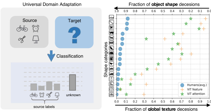
Figure 1: Left: Illustration of Universal Domain Adaptation. Right: Shape-bias Analysis. Plot shows shape-texture trade off for attention and feature in ViT and humans.

图 1: 左: 通用域自适应 (Universal Domain Adaptation) 示意图。右: 形状偏置分析。曲线图展示了 ViT 和人类在注意力机制与特征层面的形状-纹理权衡关系。

In UniDA, the primary objective is to develop a model capable of precisely categorizing target samples as one of the common classes or an "unknown" class as shown in Fig. 1 left. Existing UniDA methods aim to design a transfer ability criteria to detect common and private classes solely based on the disc rim inability of deep features [6, 7, 8, 9, 13, 27, 29, 47, 48, 50, 66]. However, over-reliance on deep features can impede model adaptation performance, as they have a strong bias towards global information like texture rather than the essential object information like shape [16, 20], which is considered by humans as the most critical cue for recognition [28]. Fortunately, recent studies have demonstrated that vision transformer (ViT) [24] exhibits a stronger shape bias than Convolutional Neural Network (CNN) [41, 55]. As shown in Fig. 1 right, we confirmed that such strong object shape bias is mainly attributed to the self-attention mechanism, verified in a similar way as [16]. Figure 2 demonstrates the attention vectors of samples accross domains. Although we can leverage the attention to focus on more object parts, the attention mismatch problem may still exist due to domain shift, which refers to the attention vectors of sameclass samples from different domains having some degree of the difference caused by potential variations in object size, orientation, and position across different domains. Attention mismatch can hinder the accurate classification of samples, especially when objects of different classes share similar sizes or positions. For example, in Figure 2, the kettle in the source domain and the flower in the target domain have more similar attention patterns. Therefore, the key challenge in utilizing attention is to effectively explore and leverage the object information embedded in attention while mitigating the negative impact of attention mismatch.

在UniDA中，主要目标是开发一个能够精确将目标样本分类为常见类别或"未知"类的模型，如图1左所示。现有UniDA方法旨在设计迁移能力标准，仅基于深度特征的判别性来检测公共类和私有类 [6, 7, 8, 9, 13, 27, 29, 47, 48, 50, 66]。然而，过度依赖深度特征会阻碍模型适应性能，因为它们对纹理等全局信息有强烈偏好，而非形状等本质对象信息 [16, 20]，而人类认为后者是最关键的识别线索 [28]。幸运的是，近期研究表明视觉Transformer (ViT) [24] 比卷积神经网络 (CNN) [41, 55] 表现出更强的形状偏好。如图1右所示，我们证实这种强烈的对象形状偏好主要归因于自注意力机制，验证方式与 [16] 类似。图2展示了跨域样本的注意力向量分布。虽然可以利用注意力聚焦更多对象部位，但由于域偏移导致的注意力失配问题仍然存在——不同域中同类样本的注意力向量会因对象尺寸、朝向和位置的潜在差异而产生一定程度的分化。注意力失配会阻碍样本的准确分类，特别是当不同类别的对象具有相似尺寸或位置时。例如图2中，源域的水壶和目标域的花朵就表现出更相似的注意力模式。因此，利用注意力的关键挑战在于：有效发掘并利用注意力中嵌入的对象信息，同时减轻注意力失配的负面影响。

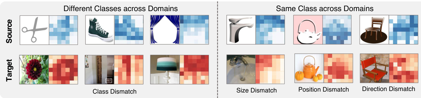
Figure 2: Attention Visualization accross domains. Attention patterns vary significantly between different classes of images. However, within the same class, attention can also exhibit variations due to differences in object size, position, and orientation. These variations are collectively referred to as attention mismatch.

图 2: 跨领域注意力可视化。不同类别图像间的注意力模式存在显著差异。然而在同一类别中，由于物体尺寸、位置和方向的差异，注意力分布也会呈现变化。这些差异统称为注意力失配 (attention mismatch)。

In this paper, we propose a novel Universal Attention Matching (UniAM) framework to address the UniDA problem by leveraging both the feature and attention information in a complementary way. Specifically, UniAM introduces a Compressive Attention Matching (CAM) approach to solve the attention mismatch problem implicitly by sparsely representing target attentions using source attention prototypes. This allows CAM to identify the most relevant attention prototype for each target sample and distinguish irrelevant private labels. Furthermore, a residual-based measurement is proposed in CAM to explicitly distinguish common and private samples across domains. By integrating attention information with features, we can mitigate the interference caused by domain shift and focus on label shift to some extent. With the guidance of CAM, the UniAM framework achieves domain-wise and category-wise common feature alignment (CFA) and target class separation (TCS). By using an adversarial loss and a source contrastive loss, CFA identifies and aligns the common features across domains, ensuring their consistency and transfer ability. On the other hand, TCS enhances the compactness of the target clusters, leading to better separation among all target classes. This is accomplished through a target contrastive loss, which encourages samples from the same target class to be closer together and farther apart from samples with other classes.

本文提出了一种新颖的通用注意力匹配(UniAM)框架，通过互补利用特征和注意力信息来解决UniDA问题。具体而言，UniAM引入压缩注意力匹配(CAM)方法，通过使用源注意力原型对目标注意力进行稀疏表示，从而隐式解决注意力失配问题。这使得CAM能够为每个目标样本识别最相关的注意力原型，并区分无关的私有标签。此外，CAM中提出基于残差的度量方法，显式区分跨域的公共样本和私有样本。通过将注意力信息与特征相结合，我们能在一定程度上减轻域偏移带来的干扰，并聚焦于标签偏移问题。

在CAM的指导下，UniAM框架实现了域级和类别级的公共特征对齐(CFA)与目标类分离(TCS)。通过对抗损失和源对比损失，CFA识别并对齐跨域公共特征，确保其一致性和迁移能力。另一方面，TCS通过目标对比损失增强目标类簇的紧密度，从而提升所有目标类间的分离度——该损失函数促使同类目标样本彼此靠近，而异类样本相互远离。

Main Contributions: (1) We propose the UniAM framework that comprehensively considers both attention and feature information, which allows for more accurate identification of common and private samples. (2) We validate the strong object bias of attention in ViT. To the best of our knowledge, we are the first to directly utilize attention in ViT for classification prediction. (3) We implicitly explore object information by sparsely reconstructing attention, enabling better common feature alignment (CFA) and target class separation (TCS). (4) We conduct extensive experiments to show that UniAM can outperform current state-ofthe-art approaches.

主要贡献：(1) 我们提出UniAM框架，全面考虑注意力与特征信息，能更精准识别共有和私有样本。(2) 我们验证了ViT中注意力机制的强目标偏向性。据我们所知，这是首次直接利用ViT中的注意力进行分类预测。(3) 通过稀疏重构注意力隐式探索目标信息，实现更好的共有特征对齐(CFA)与目标类别分离(TCS)。(4) 大量实验表明UniAM能超越当前最先进方法。

2. Related Works

2. 相关工作

2.1. Universal Domain Adaptation

2.1. 通用领域自适应

UniDA [66] does not require prior knowledge of label set relationship. To address this problem, UAN [66] proposes a criterion based on entropy and domain similarity to quantify sample transfer ability. CMU [13] follows this paradigm to detect open classes by setting the mean of three uncertain scores including entropy, consistency and confidence as a new measurement. Afterward, [27] proposes a real-time adaptive source-free UniDA method. In [47] and [29], clustering is developed to solve this problem. [31]. OVANet [48] employs a One-vs-All classifier for each class and decides known or unknown by using the output. Recent works have shifted their focus towards finding mutually nearest neighbor samples of target samples [7, 8, 9, ?] or constructing relationships between target samples and source prototypes [26, 6].

UniDA [66] 不需要预先了解标签集关系。为解决这一问题，UAN [66] 提出了一种基于熵和域相似性的准则来量化样本迁移能力。CMU [13] 沿用这一范式，通过将熵、一致性和置信度三个不确定性分数的均值作为新度量来检测开放类别。随后，[27] 提出了一种实时自适应的无源 UniDA 方法。在 [47] 和 [29] 中，聚类方法被用于解决该问题。[31]。OVANet [48] 为每个类别使用一对多分类器，并通过输出结果判定已知或未知类别。近期研究转向寻找目标样本的互最近邻样本 [7, 8, 9, ?] 或构建目标样本与源原型之间的关系 [26, 6]。

2.2. Vision Transformer

2.2. Vision Transformer

Inspired by the success of Transformer [58, 23] in the NLP field, many researchers have attempted to exploit it for solving computer vision tasks. One of the most pioneering works is Vision Transformer (ViT)[24], which decomposes input images into a sequence of fixed-size patches. Different from CNNs that rely on image-specific inductive bias, ViT takes the advantage of large-scale pre-training data and global context modeling on the entire images. Due to the outstanding performance of ViT, many approaches have been proposed based on it [54, 36, 60, 21, 37], such as Touvron et al. [54] propose DeiT, which introduces a distillation strategy specific to transformers to reduce computational costs. In general, ViT and its variants have achieved excellent results on many computer vision tasks, such as object detection [5, 76, 60], image segmentation [75, 61], and video understanding [17, 42], etc.

受Transformer [58, 23] 在自然语言处理领域成功的启发，许多研究者尝试将其应用于计算机视觉任务。最具开创性的工作之一是Vision Transformer (ViT) [24]，它将输入图像分解为固定大小的图像块序列。不同于依赖图像特定归纳偏置的CNN，ViT充分利用了大规模预训练数据和对整幅图像的全局上下文建模优势。由于ViT的卓越表现，基于它的各类方法不断涌现 [54, 36, 60, 21, 37]，例如Touvron等人 [54] 提出的DeiT通过引入针对Transformer的蒸馏策略来降低计算成本。总体而言，ViT及其变体在目标检测 [5, 76, 60]、图像分割 [75, 61] 和视频理解 [17, 42] 等计算机视觉任务中取得了优异成果。

Recently, ViT has been adopted for the DA task in several works. TVT [65] proposes an transferable adaptation module to capture disc rim i native features and achieve domain alignment. SSRT [53] formulates a comprehensive framework, which pairs a transformer backbone with a safe self-refinement strategy to navigate challenges associated with large domain gaps effectively. CDTrans [64] designs a triple-branch framework to apply self-attention and cross-attention for source-target domain feature alignment. Differently, we focus in this paper on investigating attention mechanism’s superior disc rim inability across different classes on universal domain adaptation.

最近，ViT（Vision Transformer）已被多项研究应用于领域自适应（DA）任务。TVT [65] 提出了一种可迁移适配模块，用于捕捉判别性特征并实现域对齐。SSRT [53] 构建了一个综合框架，将Transformer主干网络与安全自优化策略相结合，有效应对大域差距带来的挑战。CDTrans [64] 设计了三分支框架，通过自注意力和交叉注意力实现源-目标域特征对齐。与之不同，本文重点研究注意力机制在通用域自适应中跨类别的卓越判别能力。

2.3. Sparse Representation Classification

2.3. 稀疏表示分类

Sparse Representation Classification (SRC) [62] and Collaborative Representation Classification (CRC)[71], along with their numerous extensions [35, 63, 11, 10, 18], have been extensively investigated in the field of face recognition using single images and videos. These methods have demonstrated promising performance in the presence of occlusions and variations in illumination. By modeling the test data in terms of a sparse linear combination of a dictionary, SRC can capture non-linear relationships between features. Our UniAM is inspired by them but uses a novel measurement instead of a sparsity concentration index.

稀疏表示分类 (Sparse Representation Classification, SRC) [62] 与协同表示分类 (Collaborative Representation Classification, CRC) [71] 及其众多扩展方法 [35, 63, 11, 10, 18] 已在单图像和视频人脸识别领域得到广泛研究。这些方法在存在遮挡和光照变化的情况下表现出优异的性能。通过将测试数据建模为字典的稀疏线性组合，SRC 能够捕捉特征间的非线性关系。我们的 UniAM 受其启发，但采用了一种新颖的度量方式替代稀疏集中指数。

3. Problem Formulation and Preliminary

3. 问题表述与初步准备

3.1. Problem Formulation

3.1. 问题表述

Denoting X, Y, $\mathbb{Z}$ as the input space, label space and latent space, respectively. Elements of $\mathbb{X}$ , Y, $\mathbb{Z}$ are noted as $x,y$ and ${z}$ . Let $P{s}$ and $P_{t}$ be the source distribution and target distribution, respectively. We are given a labeled source domain $\mathbb{D}{s}={\pmb{x}{i},y_{i}}}{i=1}^{m}$ and an unlabeled target domain $\mathbb{D}{t}={\pmb{x}{i}}{i=1}^{n}$ are respectively sampled from $P_{s}$ and $P_{t}$ , where $m$ and $n$ denote the number of samples of source and target domains, respectively. Denote $\mathbb{L}_{s}$ and $\mathbb{L}_{t}$ as the label sets of the source and target domains, respectively. Let $\mathbb{L}=\mathbb{L}_{s}\cap\mathbb{L}_{t}$ be the common label set shared by both domains, while $\overline{{\mathbb{L}}}_{s}=\mathbb{L}_{s}\backslash\mathbb{L}$ and $\overline{{\mathbb{L}}}_{t}=\mathbb{L}_{t}\backslash\mathbb{L}$ be the label sets private to source and target domains, respectively. Denote $M=\left|\mathbb{L}_{s}\right|$ as the number of source labels. Universal domain adaptation aims to predict labels of target data in $\mathbb{L}$ while rejecting the target data in $\overline{{\mathbb{L}}}^{t}$ based on $\mathbb{D}_{s}$ and $\mathbb{D}_{t}$ .

记X、Y、$\mathbb{Z}$分别为输入空间、标签空间和潜在空间。$\mathbb{X}$、Y、$\mathbb{Z}$中的元素记为$x,y$和${z}$。设$P{s}$和$P_{t}$分别为源分布和目标分布。给定标记的源域$\mathbb{D}{s}={\pmb{x}{i},y_{i}}{i=1}^{m}$和未标记的目标域$\mathbb{D}{t}={\pmb{x}{i}}{i=1}^{n}$分别从$P_{s}$和$P_{t}$中采样，其中$m$和$n$分别表示源域和目标域的样本数量。记$\mathbb{L}_{s}$和$\mathbb{L}_{t}$分别为源域和目标域的标签集。设$\mathbb{L}=\mathbb{L}_{s}\cap\mathbb{L}_{t}$为两域共享的公共标签集，$\overline{{\mathbb{L}}}_{s}=\mathbb{L}_{s}\backslash\mathbb{L}$和$\overline{{\mathbb{L}}}_{t}=\mathbb{L}_{t}\backslash\mathbb{L}$分别为源域和目标域私有的标签集。记$M=\left|\mathbb{L}_{s}\right|$为源标签数量。通用域适应的目标是根据$\mathbb{D}_{s}$和$\mathbb{D}_{t}$预测$\mathbb{L}$中的目标数据标签，同时拒绝$\overline{{\mathbb{L}}}^{t}$中的目标数据。

Our overall architecture consists of a ViT-based feature extractor, an adversarial domain classifier, and a label classifier. Suppose the function for learning embedding features is $G_{f}:\mathbb{X}\rightarrow\mathbb{Z}\in\mathbb{R}^{d_{z}}$ where $d_{z}$ is the length of each feature vector, the discrimination function of the label classifier is $G_{c}:\mathbb{Z}\to\mathbb{Y}\in\mathbb{R}^{M}$ , and the function of the domain classifier is $G_{d}:\mathbb{Z}\to\mathbb{R}^{1}$ .

我们的整体架构由一个基于ViT的特征提取器、一个对抗性域分类器和一个标签分类器组成。假设学习嵌入特征的函数为 $G_{f}:\mathbb{X}\rightarrow\mathbb{Z}\in\mathbb{R}^{d_{z}}$ ，其中 $d_{z}$ 是每个特征向量的长度，标签分类器的判别函数为 $G_{c}:\mathbb{Z}\to\mathbb{Y}\in\mathbb{R}^{M}$ ，域分类器的函数为 $G_{d}:\mathbb{Z}\to\mathbb{R}^{1}$ 。

3.2. Preliminary

3.2. 初步准备

To start with, we provide an overview of the selfattention mechanism used in ViT. First, the input image ${x}$ is divided into $N$ fixed-size patches, which are linearly embedded into a sequence of vectors. Next, a special token called the class token is prepended to the sequence of image patches for classification. The resulting sequence of length $N+1$ is then projected into three matrices: queries $Q\in\mathbb{R}^{(N+1)\times d{k}}$ , keys $\dot{\boldsymbol{K}}\in\mathbb{R}^{(N+1)\times d_{k}}$ and values $V\in\mathbf{\Omega}$ R(N+1)×dv with dk and dv being the length of each query and value vector, respectively. Then, $Q$ and $\kappa$ are passed to the self-attention layer to compute the patch-to-patch similarity matrix $\pmb{A}^{(N+\bar{1})\times(N+1)}$ , which is given by

首先，我们概述ViT中使用的自注意力机制。输入图像$x$被划分为$N$个固定大小的图像块，这些块经过线性嵌入转换为向量序列。随后，一个名为分类token的特殊token被添加到图像块序列前用于分类。最终得到的长度为$N+1$的序列被投影为三个矩阵：查询矩阵$Q\in\mathbb{R}^{(N+1)\times d_{k}}$、键矩阵$\dot{\boldsymbol{K}}\in\mathbb{R}^{(N+1)\times d_{k}}$和值矩阵$V\in\mathbf{\Omega}$ R(N+1)×dv，其中$d_k$和$d_v$分别表示每个查询向量和值向量的长度。接着，$Q$和$\kappa$被送入自注意力层，计算块间相似度矩阵$\pmb{A}^{(N+\bar{1})\times(N+1)}$，其表达式为

For ease of further processing, we flatten $\pmb{A}$ into a vector $\pmb{a}\in\mathbb{R}^{(N+1)^{2}\times1}$ . It is worth noting that multiple attention heads are utilized in the self-attention mechanism. Each head outputs a separate attention, and the final attention is obtained by concatenating the vectors from all heads. As a result, the dimensionality of $\pmb{a}\in\mathbb{R}^{d_{a}\times1}$ , where $d_{a}=N_{H}\times(N+1)^{2}$ and $N_{H}$ is the number of attention heads. The utilization of multiple heads allows the model to jointly attend to information from different feature subspaces at different positions.

为便于后续处理，我们将 $\pmb{A}$ 展平为向量 $\pmb{a}\in\mathbb{R}^{(N+1)^{2}\times1}$。值得注意的是，自注意力机制中使用了多个注意力头。每个头输出独立的注意力，最终注意力通过拼接所有头的向量获得。因此，$\pmb{a}\in\mathbb{R}^{d_{a}\times1}$ 的维度为 $d_{a}=N_{H}\times(N+1)^{2}$，其中 $N_{H}$ 是注意力头的数量。多头机制使模型能够同时关注来自不同位置、不同特征子空间的信息。

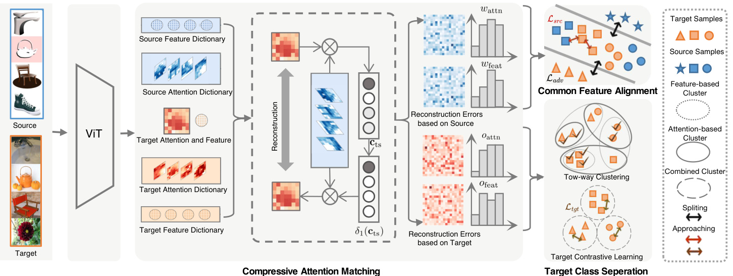
Figure 3: Illustration of the proposed UniAM framework. The framework consists of three integral components: Compressive Attention Matching (CAM), Common Feature Alignment (CFA) and Target Class Separation (TCS). At its core, CAM reconstructs all target attentions and features based on the source dictionary (with feature reconstruction omitted in the figure for simplicity), and attention and feature commonness scores $w_{\mathrm{attn}}$ and $w_{\mathrm{feat}}$ are computed from residual vectors. Then, domain- and category-wise CFA is achieved by minimizing $\mathcal{L}{a d v}$ and $\mathcal{L}{s r c}$ guided by $w_{\mathrm{attn}}$ and $w_{\mathrm{feat}}$ . Similarly, $O_{\mathrm{{attn}}}$ and $O_{\mathrm{feat}}$ are obtained by reconstructing target attentions and features based on the target dictionary in CAM. TCS performs two-way clustering from both the attention and feature views and minimizes $\mathcal{L}_{t g t}$ to achieve effective separation of target classes.

图 3: 提出的UniAM框架示意图。该框架包含三个核心组件：压缩注意力匹配(CAM)、共同特征对齐(CFA)和目标类别分离(TCS)。核心部分CAM基于源字典重建所有目标注意力和特征(图中为简化省略了特征重建)，并从残差向量计算注意力共同性分数$w_{\mathrm{attn}}$和特征共同性分数$w_{\mathrm{feat}}$。随后，在$w_{\mathrm{attn}}$和$w_{\mathrm{feat}}$的指导下，通过最小化$\mathcal{L}{a d v}$和$\mathcal{L}{s r c}$实现域级和类别级的CFA。类似地，$O_{\mathrm{{attn}}}$和$O_{\mathrm{feat}}$通过基于CAM中目标字典重建目标注意力和特征获得。TCS从注意力和特征两个视角进行双向聚类，并通过最小化$\mathcal{L}_{t g t}$实现目标类别的有效分离。

Once the attention vector $\textbf{\em a}$ is available, the corresponding $k$ -th attention prototype ${p{k}}$ is calculated by averaging all attention vectors of samples in class $k$ , which will be used in the subsequent matching process.

一旦获得注意力向量 $\textbf{\em a}$，对应的第 $k$ 个注意力原型 ${p{k}}$ 将通过计算类别 $k$ 中所有样本注意力向量的平均值得到，该原型将用于后续的匹配过程。

4. Proposed Methodology

4. 研究方法

4.1. Compressive Attention Matching

4.1. 压缩注意力匹配

Since the attention mismatch problem exists due to domain shift mentioned in Section 1, how to effectively utilize the core object information and avoid interference from redundant information poses a challenge in applying attention to UniDA. To address this challenge, compressive attention matching (CAM) is proposed to capture the most informative object structures by sparsely representing target attentions. Define the attention dictionary in CAM as the collection of source attention prototypes for efficient matching, i.e., $P_{s}=[p_{1}^{s},p_{2}^{s},\cdot\cdot\cdot,p_{M}^{s}]\in\mathbb{R}^{d_{a}\times M}$ . Definition 1 gives the definition of CAM.

由于第1节提到的领域偏移导致注意力失配问题，如何有效利用核心对象信息并避免冗余信息干扰，成为在UniDA中应用注意力机制面临的挑战。为解决该挑战，我们提出压缩注意力匹配(CAM)方法，通过稀疏化表示目标注意力来捕获最具信息量的对象结构。将CAM中的注意力字典定义为源注意力原型集合以实现高效匹配，即$P_{s}=[p_{1}^{s},p_{2}^{s},\cdot\cdot\cdot,p_{M}^{s}]\in\mathbb{R}^{d_{a}\times M}$。定义1给出了CAM的数学表述。

Definition 1 (Compressive Attention Matching). Given an attention vector $\pmb{a}{t}\in\mathbb{R}^{d{a}\times1}$ of the target sample $\scriptstyle{\pmb{x}}{t}$ and a source attention dictionary $P{s}$ , Compressive Attention Matching aims to match $\mathbf{}\mathbf{}{a{t}}$ with one prototype in $P_{s}$ to determine its commonness, which is achieved by assuming that $\mathbf{}\mathbf{}\mathbf{}\mathbf{}\mathbf{}\mathbf{}\mathbf{}\mathbf{}\mathbf{}\mathbf{}\mathbf{}\mathbf{}\mathbf{}\mathbf{}\mathbf{}\mathbf{}\mathbf{}\mathbf{}\mathbf{}\mathbf{}\mathbf{}\mathbf{}\mathbf{}\mathbf{}\mathbf{}\mathbf{}\mathbf{}\mathbf{}\mathbf{}\mathbf{}\mathbf{}\mathbf{}\mathbf{}\mathbf{}\mathbf{}\mathbf{}\mathbf{}\mathbf{}\mathbf{}\mathbf{}\mathbf{}\mathbf{}\mathbf{}\mathbf{}\mathbf{}\mathbf{}\mathbf{}\mathbf{}\mathbf{}\mathbf{}\mathbf{}\mathbf{}\mathbf{}\mathbf{}\mathbf{}\mathbf{}\mathbf{}\mathbf{}\mathbf{}\mathbf{}\mathbf{}\mathbf{}\mathbf{}\mathbf{}\mathbf{}\mathbf{}\mathbf{}\mathbf{}\mathbf{}\mathbf{}\mathbf{}\mathbf{}\mathbf{}\mathbf{}\mathbf{}\mathbf{}\mathbf{}\mathbf{}\mathbf{}\mathbf{}\mathbf{}\mathbf{}\mathbf{}\mathbf{}\mathbf{}\mathbf{}\mathbf{}\mathbf{}\mathbf{}\mathbf{}\mathbf{}\mathbf{}\mathbf{}\mathbf{}\mathbf{}\mathbf{}\mathbf{}\mathbf{}\mathbf{}\mathbf{}\mathbf{}\mathbf{}\mathbf{}\mathbf{}\mathbf{}\mathbf{}\mathbf{}\mathbf{}\mathbf{}\mathbf{}\mathbf{}\mathbf{}\mathbf{}\mathbf{}\mathbf{}\mathbf{}\mathbf{}\mathbf{}\mathbf{}\mathbf{}\mathbf{}\mathbf{}\mathbf{}\mathbf{}\mathbf{}\mathbf{}\mathbf{}\mathbf{}\mathbf{}\mathbf{}\mathbf{}\mathbf{}\mathbf{}\mathbf{}\mathbf{}\mathbf{}\mathbf{}\mathbf{}\mathbf{}\mathbf{}\mathbf{}\mathbf{}\mathbf{}\mathbf\mathbf{}\mathbf{}\mathbf{}\mathbf{}\mathbf{}\mathbf\mathbf{}\mathbf{}\mathbf{}\mathbf{}\mathbf\mathbf{}\mathbf{}\mathbf{}\mathbf\mathbf{}\mathbf{}\mathbf{}\mathbf\mathbf{}\mathbf{}\mathbf\mathbf{}\mathbf{}\mathbf{}\mathbf\mathbf{}\mathbf{}\mathbf\mathbf{}\mathbf{}\mathbf\mathbf{}\mathbf{}\mathbf\mathbf{}\mathbf{}\mathbf\mathbf{}\mathbf\mathbf{}\mathbf{}\mathbf\mathbf{}\mathbf}\mathbf{\mathbf}\mathbf{}\mathbf\mathbf{}\mathbf{}\mathbf\mathbf{}\mathbf\mathbf{}\mathbf\mathbf{}\mathbf\mathbf{}\mathbf\mathbf{}\mathbf\mathbf{}\mathbf\mathbf{}\mathbf\mathbf{}\mathbf}\mathbf{\mathbf}\mathbf{\mathbf}\mathbf{\mathbf}\mathbf\mathbf{}\mathbf\mathbf{}\mathbf\mathbf{}\mathbf\mathbf{}\mathbf\mathbf{}\mathbf\mathbf\mathbf{}\mathbf\mathbf{}\mathbf\mathbf}\mathbf{\mathbf}\mathbf{\mathbf}\mathbf\mathbf{}\mathbf\mathbf$ can be approximated by a linear combination of $P_{s}$ :

定义 1 (压缩注意力匹配)。给定目标样本 $\scriptstyle{\pmb{x}}{t}$ 的注意力向量 $\pmb{a}{t}\in\mathbb{R}^{d_{a}\times1}$ 和源注意力字典 $P_{s}$，压缩注意力匹配旨在将 $\mathbf{}\mathbf{}{a{t}}$ 与 $P_{s}$ 中的一个原型进行匹配以确定其共性，这是通过假设 $\mathbf{}\mathbf{}\mathbf{}\mathbf{}\mathbf{}\mathbf{}\mathbf{}\mathbf{}\mathbf{}\mathbf{}\mathbf{}\mathbf{}\mathbf{}\mathbf{}\mathbf{}\mathbf{}\mathbf{}\mathbf{}\mathbf{}\mathbf{}\mathbf{}\mathbf{}\mathbf{}\mathbf{}\mathbf{}\mathbf{}\mathbf{}\mathbf{}\mathbf{}\mathbf{}\mathbf{}\mathbf{}\mathbf{}\mathbf{}\mathbf{}\mathbf{}\mathbf{}\mathbf{}\mathbf{}\mathbf{}\mathbf{}\mathbf{}\mathbf{}\mathbf{}\mathbf{}\mathbf{}\mathbf{}\mathbf{}\mathbf{}\mathbf{}\mathbf{}\mathbf{}\mathbf{}\mathbf{}\mathbf{}\mathbf{}\mathbf{}\mathbf{}\mathbf{}\mathbf{}\mathbf{}\mathbf{}\mathbf{}\mathbf{}\mathbf{}\mathbf{}\mathbf{}\mathbf{}\mathbf{}\mathbf{}\mathbf{}\mathbf{}\mathbf{}\mathbf{}\mathbf{}\mathbf{}\mathbf{}\mathbf{}\mathbf{}\mathbf{}\mathbf{}\mathbf{}\mathbf{}\mathbf{}\mathbf{}\mathbf{}\mathbf{}\mathbf{}\mathbf{}\mathbf{}\mathbf{}\mathbf{}\mathbf{}\mathbf{}\mathbf{}\mathbf{}\mathbf{}\mathbf{}\mathbf{}\mathbf{}\mathbf{}\mathbf{}\mathbf{}\mathbf{}\mathbf{}\mathbf{}\mathbf{}\mathbf{}\mathbf{}\mathbf{}\mathbf{}\mathbf{}\mathbf{}\mathbf{}\mathbf{}\mathbf{}\mathbf{}\mathbf{}\mathbf{}\mathbf{}\mathbf{}\mathbf{}\mathbf{}\mathbf{}\mathbf{}\mathbf{}\mathbf{}\mathbf{}\mathbf{}\mathbf{}\mathbf{}\mathbf{}\mathbf{}\mathbf{}\mathbf{}\mathbf{}\mathbf{}\mathbf{}\mathbf{}\mathbf{}\mathbf{}\mathbf{}\mathbf{}\mathbf\mathbf{}\mathbf{}\mathbf{}\mathbf{}\mathbf{}\mathbf\mathbf{}\mathbf{}\mathbf{}\mathbf{}\mathbf\mathbf{}\mathbf{}\mathbf{}\mathbf\mathbf{}\mathbf{}\mathbf{}\mathbf\mathbf{}\mathbf{}\mathbf\mathbf{}\mathbf{}\mathbf{}\mathbf\mathbf{}\mathbf{}\mathbf\mathbf{}\mathbf{}\mathbf\mathbf{}\mathbf{}\mathbf\mathbf{}\mathbf{}\mathbf\mathbf{}\mathbf\mathbf{}\mathbf{}\mathbf\mathbf{}\mathbf}\mathbf{\mathbf}\mathbf{}\mathbf\mathbf{}\mathbf{}\mathbf\mathbf{}\mathbf\mathbf{}\mathbf\mathbf{}\mathbf\mathbf{}\mathbf\mathbf{}\mathbf\mathbf{}\mathbf\mathbf{}\mathbf\mathbf{}\mathbf}\mathbf{\mathbf}\mathbf{\mathbf}\mathbf{\mathbf}\mathbf\mathbf{}\mathbf\mathbf{}\mathbf\mathbf{}\mathbf\mathbf{}\mathbf\mathbf{}\mathbf\mathbf\mathbf{}\mathbf\mathbf{}\mathbf\mathbf}\mathbf{\mathbf}\mathbf{\mathbf}\mathbf\mathbf{}\mathbf\mathbf$ 可以近似为 $P_{s}$ 的线性组合来实现：

where the coefficient vector $\pmb{c}{t s}\in\mathbb{R}^{M\times1}$ satisfies a sparsity constraint in order to achieve a compressive representation. Based on $\mathbf{\Delta}{c_{t s},\textit{\mathbf{x}}_{t}}$ is regarded as belonging to common classes from an attention perspective when the following inequality is satisfied:

其中系数向量 $\pmb{c}{t s}\in\mathbb{R}^{M\times1}$ 需满足稀疏性约束以实现压缩表示。当满足以下不等式时，基于 $\mathbf{\Delta}{c_{t s},\textit{\mathbf{x}}_{t}}$ 从注意力角度被视为属于常见类别：

$w_{a t t n}(\cdot)$ indicates a measurement to evaluate the commonness of $\scriptstyle{\pmb{x}}_{t}$ which is defined later and $\delta$ is a threshold.

$w_{a t t n}(\cdot)$ 表示评估 $\scriptstyle{\pmb{x}}_{t}$ 常见程度的度量标准 (该定义将在后文给出) ，$\delta$ 为阈值。

Why Compressive Attention Matching is desirable? By enforcing sparsity on the coefficients in CAM, we can obtain a compressive representation of the attention vectors, which facilitates the extraction and utilization of lowdimensional structures embedded in high-dimensional attention vectors. In the context of UniDA, this compressive representation enables us to identify the most relevant attention prototype for each target sample and distinguish irrele- vant private labels, which is crucial for achieving effective common and private class detection. Therefore, CAM with sparse coefficients plays a vital role in solving UniDA.

为什么压缩注意力匹配(CAM)是理想的？通过对CAM中的系数施加稀疏性，我们可以获得注意力向量的压缩表示，这有助于提取和利用嵌入高维注意力向量中的低维结构。在UniDA(通用域适应)的背景下，这种压缩表示使我们能够为每个目标样本识别最相关的注意力原型，并区分无关的私有标签，这对于实现有效的公共类和私有类检测至关重要。因此，具有稀疏系数的CAM在解决UniDA问题中起着关键作用。

To solve Eq. 2 in CAM, the coefficient vector $c_{t s}$ is estimated by:

为求解CAM中的方程2，系数向量$c_{t s}$通过以下方式估计：

where $||\cdot||{p}$ denotes $\ell{p}$ -norm. The $\ell_{1}$ -minimization term in Eq. 3 yields a sparse solution, which enforces that $c_{t s}$ has only a small number of non-zero coefficients.

其中 $||\cdot||{p}$ 表示 $\ell{p}$ 范数。式(3)中的 $\ell_{1}$ 最小化项会产生稀疏解，这强制要求 $c_{t s}$ 仅具有少量非零系数。

Then we can compute the class reconstruction error vector $\pmb{r}{t s}\in\mathbb{R}^{M}$ for each target sample using the sparse matrix $c{t s}$ . The $k$ -th entry of $\mathbf{\Delta}{r{t s}}$ can be represented:

然后我们可以利用稀疏矩阵 $c_{t s}$ 计算每个目标样本的类别重构误差向量 $\pmb{r}{t s}\in\mathbb{R}^{M}$ 。$\mathbf{\Delta}{r_{t s}}$ 的第 $k$ 个分量可表示为:

where $\delta_{k}(\mathbf{\sigma}{c{t s}})$ is a one-hot vector with the $k$ -th entry in $c_{t s}$ being non-zero while setting all other entries to zero. If $\scriptstyle{\pmb{x}}{t}$ corresponds to a common class $k$ , then the reconstruction error corresponding to class $k$ . $r{t s}(k)$ should be much lower than that corresponding to the other classes. Conversely, if $\mathbf{\boldsymbol{x}}{t}$ belongs to a private class, the difference between elements of the entire reconstruction error vector $\mathbf{\Delta}{r_{t s}}$ should be relatively small, without a significant difference between the errors corresponding to different classes.

其中 $\delta_{k}(\mathbf{\sigma}{c{t s}})$ 是一个独热向量 (one-hot vector) ，其 $c_{t s}$ 中的第 $k$ 个条目为非零值，而其他所有条目均为零。如果 $\scriptstyle{\pmb{x}}{t}$ 对应于一个常见类别 $k$ ，那么对应于类别 $k$ 的重构误差 $r{t s}(k)$ 应该远低于其他类别对应的重构误差。相反，如果 $\mathbf{\boldsymbol{x}}{t}$ 属于一个私有类别，则整个重构误差向量 $\mathbf{\Delta}{r_{t s}}$ 中各元素之间的差异应该相对较小，不同类别对应的误差之间没有显著差异。

As a result, the reconstruction error vector $\mathbf{\Delta}{r{t s}}$ is a crucial component in CAM. It serves as the foundation for the design of the measurement $w_{\mathrm{attn}}(\cdot)$ in Definition 1 called Attention Commonness Degree (ACD), defined as belows:

因此，重建误差向量 $\mathbf{\Delta}{r{t s}}$ 是 CAM 中的关键组成部分。它作为定义 1 中测量 $w_{\mathrm{attn}}(\cdot)$ 的基础，称为注意力共性度 (ACD)，定义如下：

Definition 2 (Attention Commonness Degree). Given the residual vector $\mathbf{\Delta}{r{t s}}$ of $\mathbf{\boldsymbol{x}}_{t}$ , the ACD is defined as the difference between the average of non-matched errors and matched errors:

定义 2 (注意力共性度). 给定 $\mathbf{\boldsymbol{x}}{t}$ 的残差向量 $\mathbf{\Delta}{r_{t s}}$ ，ACD 定义为非匹配误差与匹配误差平均值之差:

where match $(\pmb{r}{t s})=\pmb{r}{t s}(\hat{y})$ , $\begin{array}{r}{\hat{y}=\arg\operatorname*{min}{k}r{t s}(k)}\end{array}$ and non-match $\left(\pmb{r}_{t s}\right)$ is the average of reconstruction errors excepting $\hat{y}$ .

其中匹配 $(\pmb{r}{t s})=\pmb{r}{t s}(\hat{y})$ ， $\begin{array}{r}{\hat{y}=\arg\operatorname*{min}{k}r{t s}(k)}\end{array}$ ，非匹配 $\left(\pmb{r}_{t s}\right)$ 是除 $\hat{y}$ 外重建误差的平均值。

Remark 1. ACD measures the degree of commonness for a target sample $\scriptstyle{\pmb{x}}{t}$ , which represents the probability of belonging to common classes. A higher ACD value indicates a larger difference between non-matched and matched errors, suggesting the presence of an attention prototype similar to $\scriptstyle{\pmb{x}}{t}$ , and consequently, a higher degree of sample commonness. Conversely, a smaller ACD value implies a similar reconstruction error between $\scriptstyle{\boldsymbol{x}}_{t}$ and all source prototypes, indicating a lower degree of sample commonness and a higher degree of private ness.

备注1. ACD衡量目标样本$\scriptstyle{\pmb{x}}{t}$的共性程度，表示其属于常见类的概率。ACD值越高，非匹配误差与匹配误差之间的差异越大，表明存在与$\scriptstyle{\pmb{x}}{t}$相似的注意力原型，因此样本共性程度越高。反之，ACD值越小，说明$\scriptstyle{\boldsymbol{x}}_{t}$与所有源原型之间的重构误差相近，表明样本共性程度较低而私有性程度较高。

To complement the attention information, we retain features that reflect global information. The target feature $z_{t}$ can be also represented by the linear span of source feature prototypes $Q_{s}=[\pmb{q}{1}^{s},\pmb{q}{2}^{s},\cdot\cdot\cdot,\pmb{q}{M}^{s}]$ , i.e., ${z{t}=Q_{s}c_{t s}}$ . The corresponding residual vector $r_{t s}^{\prime}(k)$ is computed based on $c_{t s}$ . The Feature Commonness Degree (FCD) can be defined as $w_{\mathrm{feat}}({\pmb x}_{t})=\mathrm{non}\mathrm{-match}({\pmb r}_{t s}^{\prime})-\mathrm{match}({\pmb r}_{t s}^{\prime}).$ .

为补充注意力信息，我们保留了反映全局信息的特征。目标特征$z_{t}$也可表示为源特征原型$Q_{s}=[\pmb{q}{1}^{s},\pmb{q}{2}^{s},\cdot\cdot\cdot,\pmb{q}{M}^{s}]$的线性组合，即${z{t}=Q_{s}c_{t s}}$。对应的残差向量$r_{t s}^{\prime}(k)$基于$c_{t s}$计算得出。特征共性度(FCD)可定义为$w_{\mathrm{feat}}({\pmb x}_{t})=\mathrm{non}\mathrm{-match}({\pmb r}_{t s}^{\prime})-\mathrm{match}({\pmb r}_{t s}^{\prime}).$

It is worth noting that by replacing $P_{s}$ in Definition 2 with the target dictionary $P_{t}$ , we can obtain compressive representations of target attentions towards $P_{t}$ . This leads to a score similar to that in Definition 2, denoted as $O_{\mathrm{{atth}}}$ . The same goes for $O_{\mathrm{feat}}$ . These scores can facilitate determining the probability that two target samples belong to the same class, more details will be provided in Section 4.3.

值得注意的是，将定义2中的$P_{s}$替换为目标字典$P_{t}$，我们可以获得针对$P_{t}$的目标注意力压缩表示。这将产生一个类似于定义2中的分数，记为$O_{\mathrm{{atth}}}$。同理适用于$O_{\mathrm{feat}}$。这些分数有助于确定两个目标样本属于同一类别的概率，更多细节将在4.3节中提供。

In summary, both attention and feature characteristics are important factors that affect the perception of similarity between different categories. Attention captures the structural properties of objects, while feature captures the appearance properties of the global images. Therefore, we can achieve a more comprehensive and accurate private class detection model that takes into account both object information and global information.

总之，注意力和特征特性都是影响不同类别间相似性感知的重要因素。注意力捕捉物体的结构属性，而特征捕捉全局图像的外观属性。因此，我们可以构建一个更全面、更准确的私有类别检测模型，兼顾物体信息和全局信息。

4.2. Common Feature Alignment

4.2. 通用特征对齐

To identify and align the common class features across domains, we propose a domain-wise and category-wise Common Feature Alignment (CFA) technique, which considers both attention and feature information.

为了识别并对齐跨领域的共同类别特征，我们提出了一种基于领域和类别的共同特征对齐(Common Feature Alignment, CFA)技术，该技术同时考虑了注意力机制和特征信息。

Domain-wise Alignment. To achieve domain-wise alignment, we first propose a residual-based transfer ability score $d_{\mathrm{t}}$ measuring the probability that the target sample belongs to the common classes, which can be summarized as:

领域对齐。为实现领域对齐，我们首先提出一种基于残差的迁移能力评分 $d_{\mathrm{t}}$ ，用于衡量目标样本属于公共类的概率，其计算公式可表示为：

where $\lambda$ is a hyper parameter balancing their contribution. Meanwhile, to measure the probability that the source sample $\pmb{x}{s}$ with label $j$ belongs to the common label set, we compute $\boldsymbol{w}{j}^{s}$ with the sum of all target samples’ attention and feature reconstruction errors respectively, i.e.

其中 $\lambda$ 是平衡两者贡献的超参数。同时，为了衡量带标签 $j$ 的源样本 $\pmb{x}{s}$ 属于公共标签集的概率，我们分别计算所有目标样本的注意力之和与特征重构误差之和来得到 $\boldsymbol{w}{j}^{s}$，即

where $r_{t s}^{i}$ indicates the reconstruction error of the $i$ -th target sample. The operator $\begin{array}{r}{\sigma({\pmb r})=\frac{{\pmb r}-m i n({\pmb r})}{m a x({\pmb r})-m i n({\pmb r})}}\end{array}$ max(−r)−min(r) refers to the normalization sum of all target attention or feature residual vectors. A larger value of $w_{j}^{s}$ indicates a higher probability that the source label $j$ belongs to the common label set, while lower values suggest that it is more likely to be a source private label. It is worth noting that source samples with the same label are assigned the same weight.

其中 $r_{t s}^{i}$ 表示第 $i$ 个目标样本的重构误差。运算符 $\begin{array}{r}{\sigma({\pmb r})=\frac{{\pmb r}-m i n({\pmb r})}{m a x({\pmb r})-m i n({\pmb r})}}\end{array}$ max(−r)−min(r) 表示所有目标注意力或特征残差向量的归一化总和。$w_{j}^{s}$ 值越大，表明源标签 $j$ 属于公共标签集的概率越高；值越小，则越可能是源私有标签。值得注意的是，具有相同标签的源样本会被赋予相同的权重。

Based on the above two weights, we can derive a domain-wise adversarial loss that aligns the common classes across domains as follows:

基于上述两种权重，我们可以推导出一个跨域对抗损失函数，用于对齐不同领域间的共有类别，具体如下：

In addition, to avoid being interfered with the knowledge of source private samples, we employ an indicator as the weight for the weighted cross-entropy loss $\mathcal{L}_{\mathrm{cls}}$ for the source domain, as shown below:

此外，为避免受到源私有样本知识的干扰，我们采用一个指示器作为源域加权交叉熵损失 $\mathcal{L}_{\mathrm{cls}}$ 的权重，如下所示：

where ${l}_{c e}$ is the standard cross-entropy loss.

其中 ${l}_{c e}$ 是标准交叉熵损失。

Category-wise Alignment. To enhance the source discriminability and align the common features from a categorywise perspective across domains, we propose a contrastive

类别对齐。为了增强源可辨别性并从跨领域的类别视角对齐共有特征，我们提出了一种对比式

Thus the category-wise common feature alignment can be improved by minimizing the source contrastive loss $\mathcal{L}_{\mathrm{src}}$ :

因此，通过最小化源对比损失 $\mathcal{L}_{\mathrm{src}}$ 可以改进类别间共同特征的对齐：

with

与

4.3. Target Class Seperation

4.3. 目标类别分离

To better distinguish the common and private classes in the target domain, we propose a Target Class Separation (TCS) technique. As mentioned in Section 4.1, we can construct a CAM problem based on the target attention dictionary $P_{t}$ . As the target labels are unknown, $P_{t}=[p_{1}^{t},p_{2}^{t}$ , $\cdot\cdot,\pmb{p}{K}^{t}]\in\mathbb{R}^{d{a}\times K}$ is initialized by performing traditional K-means algorithm on target attentions ${{\pmb a}{t}^{i}}{i=1}^{n}$ , where $K$ is pre-defined. In the subsequent attention clustering process, we calculate the residual vector $\pmb{r}_{t t}~\in\mathbb{R}^{K}$ and use it as a metric for measuring the distance between samples, which allows for dynamically update $P_{t}$ . Iterative ly refining $P_{t}$ makes it more reliable and disc rim i native. Meanwhile, the feature clustering based on the target feature dictionary $Q_{t}=[\pmb{q}_{1}^{t},\pmb{q}_{2}^{t},\cdot\cdot\cdot,\pmb{q}_{K}^{t}]\in\mathbb{R}^{d_{z}\times K}$ is also performed. After the two-way clustering, each target sample $\pmb{x}_{i}^{t}$ is assigned two cluster indexes $\hat{c}_{i}$ and $\hat{c}_{i}^{\prime}$ from attention and feature view like Fig. ?? depicted. The final soft pseudo label $o_{c,i}$ determining whether $\scriptstyle{\boldsymbol{x}}_{i}$ belong to the $c$ -th cluster is obtained based on these two cluster indexes, similar to $w_{i,j}$ . Based on $o_{i,j}$ , the target contrastive loss $\mathcal{L}_{\mathrm{tgt}}$ is computed as follows:

为了更好地区分目标域中的公共类和私有类，我们提出了一种目标类分离 (TCS) 技术。如第4.1节所述，我们可以基于目标注意力字典 $P_{t}$ 构建一个CAM问题。由于目标标签未知， $P_{t}=[p_{1}^{t},p_{2}^{t}$ , $\cdot\cdot,\pmb{p}{K}^{t}]\in\mathbb{R}^{d{a}\times K}$ 通过在对目标注意力 ${{\pmb a}{t}^{i}}{i=1}^{n}$ 执行传统K-means算法进行初始化，其中 $K$ 是预定义的。在后续的注意力聚类过程中，我们计算残差向量 $\pmb{r}_{t t}~\in\mathbb{R}^{K}$ 并将其用作衡量样本间距离的度量，从而动态更新 $P_{t}$ 。通过迭代优化 $P_{t}$ ，使其更加可靠且具有判别性。同时，基于目标特征字典 $Q_{t}=[\pmb{q}_{1}^{t},\pmb{q}_{2}^{t},\cdot\cdot\cdot,\pmb{q}_{K}^{t}]\in\mathbb{R}^{d_{z}\times K}$ 的特征聚类也在进行。经过双向聚类后，每个目标样本 $\pmb{x}_{i}^{t}$ 会被分配两个聚类索引 $\hat{c}_{i}$ 和 $\hat{c}_{i}^{\prime}$ ，分别来自注意力和特征视图，如图??所示。最终确定 $\scriptstyle{\boldsymbol{x}}_{i}$ 是否属于第 $c$ 个聚类的软伪标签 $o_{c,i}$ 基于这两个聚类索引获得，类似于 $w_{i,j}$ 。基于 $o_{i,j}$ ，目标对比损失 $\mathcal{L}_{\mathrm{tgt}}$ 计算如下：

with

与

where $o_{i,j}=o_{c,i}\cdot o_{c,j}$ is the probability weight determining whether $\boldsymbol{x}{i}$ and $\pmb{x}{j}$ belong to the same cluster $c$ . By minimizing $\mathcal{L}_{\mathrm{tgt}}$ , we can enhance the compactness of target clusters making a better separation among target classes.

其中 $o_{i,j}=o_{c,i}\cdot o_{c,j}$ 是决定 $\boldsymbol{x}{i}$ 和 $\pmb{x}{j}$ 是否属于同一聚类 $c$ 的概率权重。通过最小化 $\mathcal{L}_{\mathrm{tgt}}$，我们可以增强目标聚类的紧凑性，从而在目标类别间实现更好的分离。

4.4. Overall Framework

4.4. 总体框架

Overall, our framework is jointly optimized with four terms, i.e., cross-entropy loss $\mathcal{L}{\mathrm{cls}}$ , adversarial loss $\mathcal{L}{\mathrm{adv}}$ , source and target contrastive loss $\mathcal{L}{\mathrm{src}}$ and $\mathcal{L}{\mathrm{tgt}}$ as shown in Fig. 3,

总体而言，我们的框架通过四项联合优化目标实现协同训练，即交叉熵损失 $\mathcal{L}{\mathrm{cls}}$、对抗损失 $\mathcal{L}{\mathrm{adv}}$、源域对比损失 $\mathcal{L}{\mathrm{src}}$ 以及目标域对比损失 $\mathcal{L}{\mathrm{tgt}}$，如图 3 所示。

where $\eta_{1}$ and $\eta_{2}$ are set as 0.5 to balance each loss component. In the testing phase, given each input target sample $\scriptstyle{\boldsymbol{x}}{t}$ , we compute $w{t}$ in (6). For those samples that satisfy $w_{t}<\beta$ are assigned with the predicted source class, where $\beta$ is a validated threshold. Otherwise, the samples are marked as unknown.

其中 $\eta_{1}$ 和 $\eta_{2}$ 设为0.5以平衡各损失项。在测试阶段，给定每个输入目标样本 $\scriptstyle{\boldsymbol{x}}{t}$ ，我们计算(6)式中的 $w{t}$ 。对于满足 $w_{t}<\beta$ 的样本，将其归类为预测的源类别，其中 $\beta$ 为验证阈值。其余样本则标记为未知类别。

5. Experiment Results

5. 实验结果

5.1. Experimental Setup

5.1. 实验设置

Datasets. We perform experiments on Office-31 [46], Office-Home [59], VisDA2017 [45] and DomainNet [44] datasets. Office-31 consists of three domains: Amazon (A), DSLR (D) and Webcam (W). Each domain contains 31 categories. Office-Home is a dataset made up of 65 different categories from four domains: Artistic (Ar), Clipart (Cl), Product $(\mathrm{Pr})$ and Real-world images (Rw). VisDA2017 is a dataset with a single source and target domain testing the ability to perform transfer learning from synthetic images to natural images. The dataset has 12 categories in each domain. We conduct experiments on three subsets from it, i.e., Painting (P), Real (R), and Sketch (S). For a fair comparison, we follow the same dataset split as [66] for the first three dataset and [13] for the last dataset.

数据集。我们在Office-31 [46]、Office-Home [59]、VisDA2017 [45]和DomainNet [44]数据集上进行实验。Office-31包含三个域：Amazon (A)、DSLR (D)和Webcam (W)，每个域包含31个类别。Office-Home由四个域的65个不同类别组成：艺术图像(Ar)、剪贴画(Cl)、产品图像$(\mathrm{Pr})$和真实世界图像(Rw)。VisDA2017是测试从合成图像到自然图像迁移学习能力的单源单目标域数据集，每个域包含12个类别。我们从中选取三个子集进行实验：绘画图像(P)、真实图像(R)和素描图像(S)。为公平比较，前三个数据集采用与[66]相同的划分方式，最后一个数据集采用[13]的划分方式。

Evaluation Protocols. We evaluate all methods using Hscore [13]. H-score is the harmonic mean of the accuracy of common classes and the accuracy of the “unknown” classes, which can make a trade-off between the accuracy of known and unknown classes.

评估协议。我们使用Hscore [13]评估所有方法。H-score是常见类准确率和"未知"类准确率的调和平均数，可以在已知类和未知类准确率之间取得平衡。

Implementation Details The method is implemented in Pytorch using a ViT-base model with $16\times16$ input patch size (or ViT-B/16) [24], pretrained on ImageNet [12]), as the backbone feature extractor. The transformer encoder of ViT-B/16 contains a total of 12 Transformer layers. The label classifier consists of a fully connected network with BatchNorm [22]. The domain disc rim in at or is a three-layer MLP with ReLU activation s. We train all models using a minibatch Stochastic Gradient Descent (SGD) optimizer with a momentum of 0.9 and a weight decay of $5\times10^{-4}$ . The learning rate decays by a factor of $\left(1+\alpha i/N\right)^{-\beta}$ , where $i$ and $N$ respectively denote the current iteration and the global iteration. The batch size is set to 36. We initialize the initial learning rate to 0.01 for Office-31 and OfficeHome, while set 0.001 for VisDA2017 and DomainNet. For the regular iz ation hyper parameters, we set $\gamma~=~100$ and $\lambda=0.3$ for all dataset. For the decision threshold, we set $\alpha=0.85$ and $\beta=1.0$ for all dataset in UniDA and OSDA. In PDA, we set $\alpha=0.8$ for all dataset except $\alpha=0.85$ in the Office-31 W2A task. For the pre-defined number of target prototypes, a larger size of the target domain indicates a larger $K$ . Therefore, we empirically set $K=50$ for Office-31, $K=150$ for Office-Home, $K=500$ for VisDA, $K=1000$ for DomainNet.

实现细节
该方法基于Pytorch框架实现，采用在ImageNet [12]上预训练的ViT-base模型（输入块尺寸为$16\times16$，即ViT-B/16）[24]作为主干特征提取器。ViT-B/16的Transformer编码器共包含12层Transformer结构。标签分类器由带BatchNorm [22]的全连接网络构成，域判别器为具有ReLU激活函数的三层MLP。所有模型均使用小批量随机梯度下降(SGD)优化器进行训练，动量设为0.9，权重衰减为$5\times10^{-4}$。学习率按$\left(1+\alpha i/N\right)^{-\beta}$公式衰减，其中$i$和$N$分别表示当前迭代次数和全局迭代次数。批处理大小设置为36，Office-31和OfficeHome数据集的初始学习率设为0.01，VisDA2017和DomainNet数据集设为0.001。正则化超参数方面，所有数据集均设置$\gamma~=~100$和$\lambda=0.3$。决策阈值在UniDA和OSDA任务中统一设为$\alpha=0.85$和$\beta=1.0$；PDA任务中除Office-31的W2A任务（设为$\alpha=0.85$）外，其余数据集均设为$\alpha=0.8$。目标原型数量$K$根据目标域规模设定：Office-31取$K=50$，Office-Home取$K=150$，VisDA取$K=500$，DomainNet取$K=1000$。

Table 1: H-score $(%)$ on Office-31 and DomainNet

表 1: Office-31 和 DomainNet 上的 H-score $(%)$

方法	Office-31							DomainNet
	A2W	D2W	W2D	A2D	D2A	W2A	Avg	P2R	R2P	P2S	S2P	R2S	S2R	Avg
ResNet [19]	47.92	54.94	28.34	26.95	26.95	26.89	29.74	28.15
DANN [15]	48.82	52.73	54.87	50.18	47.69	49.33	50.60	31.18	29.33	27.84	27.84	27.77	30.84	29.13
OSBP [50]	50.23	55.53	57.20	51.14	49.75	50.16	52.34	33.60	33.03	30.55	30.53	30.61	33.65	32.00
UAN [66]	58.61	70.62	71.42	59.68	60.11	60.34	63.46	41.85	43.59	39.06	38.95	38.73	43.69	40.98
CMU [13]	67.33	79.32	80.42	68.11	71.42	72.23	50.78	52.16	45.12	44.82	45.64	50.97	48.25	73.14
DCC [29]	78.54	79.29	88.58	88.50	70.18	75.87	80.16	56.90	50.25	43.66	44.92	43.31	56.15	49.20
OVANet [48]	79.45	95.43	94.35	85.67	80.43	84.23	86.59	56.0	51.7	47.1	47.4	44.9	57.2	50.7
UniOT [6]	89.16	98.93	96.87	86.35	89.85	88.08	91.54	59.30	47.79	51.79	46.81	48.32	58.25	52.04
OVANet*	ViT	87.75	93.14	85.72	82.96	92.67	91.25	88.92	71.24	61.14	51.28	55.30	47.51	66.48	58.83
UniOT*	ViT	96.35	99.13	99.43	88.40	89.67	93.81	94.47	72.40	59.47	49.30	56.86	47.38	69.43	59.14
Ours		95.46	99.62	99.81	95.28	92.35	93.23	95.95	73.87	60.89	52.31	59.98	51.41	70.68	61.52

Table 2: H-score $(%)$ on Office-Home and VisDA2017

表 2: Office-Home 和 VisDA2017 上的 H-score $(%)$

方法	Office-Home														VisDA
	Ar2Cl	Ar2Pr	Ar2Rw	CI2Ar	C12Pr	C12Rw	Pr2Ar	Pr2Cl	Pr2Rw	Rw2Ar	Rw2Cl	Rw2Pr	Avg	S2R
ResNet [19]	44.65	48.04	50.13	46.64	46.91	48.96	47.47	43.17	50.23	48.45	44.76	48.43	47.32	25.44
DANN [15]	42.36	48.02	48.87	45.48	46.47	48.37	45.75	42.55	48.70	47.61	42.67	47.40	46.19	25.65
OSBP[50]	39.59	45.09	46.17	45.70	45.24	46.75	45.26	40.54	45.75	45.08	41.64	46.90	44.48	27.31
UAN [66]	51.64	51.70	54.30	61.74	57.63	61.86	50.38	47.62	61.46	62.87	52.61	65.19	56.58	30.47
CMU[13]	56.02	56.93	59.15	66.95	64.27	67.82	54.72	51.09	66.39	68.24	57.89	69.73	61.60	34.64
DCC [29]	57.97	54.05	58.01	74.64	70.62	77.52	64.34	73.60	74.94	80.96	75.12	80.38	70.18	43.02
OVANet[48]	62.81	75.54	78.59	70.72	68.78	75.03	71.27	58.64	80.52	76.09	64.13	78.91	71.75	53.10
UniOT [6]	67.27	80.54	86.03	73.51	77.33	84.28	75.54	63.33	85.99	77.77	65.37	81.92	76.57	57.32
OVANet*	ViT	58.09	86.06	89.38	81.86	81.03	86.22	84.49	57.06	88.54	83.67	57.32	86.67	77.45	56.98
UniOT*	63.77	88.19	90.23	74.99	81.02	84.55	78.91	61.29	87.60	82.38	63.70	88.30	78.40	63.25
Ours	72.04	87.07	90.67	80.30	82.39	79.81	85.02	68.35	88.98	85.44	72.11	86.12	81.68	65.18

5.2. Comparison Baselines

5.2. 对比基线

Follow the previous existing works [13], we compare our method with (1) ResNet [19], (2) close-set domain adaptation: DANN [15], (3) partial domain adaptation: PADA [4], ETN [3], $\mathrm{BA^{3}U S}$ [30] (4) open set domain adaptation: OSBP [50], STA [32], ROS [2]. (5)universal domain adaptation: UAN [66], CMU [13], DANCE [47], DCC [29], OVANet [48], UniOT [6], GATE [9]. We use some results from [9]. In all experiments, we assume that none of the UniDA methods have prior knowledge of category shift, while baselines tailored for each setting consider this prior.

遵循先前已有工作[13]，我们将本方法与以下方法进行对比：(1) ResNet[19]；(2) 闭集域适应：DANN[15]；(3) 部分域适应：PADA[4]、ETN[3]、$\mathrm{BA^{3}U S}$[30]；(4) 开集域适应：OSBP[50]、STA[32]、ROS[2]；(5) 通用域适应：UAN[66]、CMU[13]、DANCE[47]、DCC[29]、OVANet[48]、UniOT[6]、GATE[9]。部分结果引自[9]。所有实验中，我们假设UniDA方法均无类别偏移的先验知识，而为各场景定制的基线方法则考虑此先验。

5.3. Comparison Results

5.3. 对比结果

The experimental results for the Office-31, Office-Home, VisDA2017, and DomainNet datasets are presented in Table 1 and Table 2, which demonstrate that our proposed UniAM framework outperforms the state-of-the-art approaches in all benchmarks, as evaluated by the H-score metric. Additionally, to ensure a fair comparison, we conducted experiments by replacing the backbone of OVANet and UniOT with ViT, marked as $\star$ . The proposed method consistently surpasses these ViT-based methods by a large margin. This indicates that our approach does not solely rely on using ViT as the backbone, but rather it fully exploits the advantage of the attention mechanism in ViT for UniDA tasks to achieve such superior performance.

Office-31、Office-Home、VisDA2017和DomainNet数据集的实验结果如表1和表2所示。实验表明，在H-score指标评估下，我们提出的UniAM框架在所有基准测试中都优于现有最先进方法。此外，为确保公平比较，我们将OVANet和UniOT的主干网络替换为ViT（标记为$\star$）进行实验。所提方法始终以显著优势超越这些基于ViT的方法，这表明我们的性能优势并非单纯依赖ViT主干网络，而是充分挖掘了ViT中注意力机制在UniDA任务中的优势。

Figure 4: (a) Effectiveness on different label set relationships. Our method consistently outperforms all comparative approaches across various settings of $\overline{{\mathbb{L}}}^{t}$ . (b) Effectiveness of varying decision threshold $\alpha$ and $\beta$ . Even when both $\alpha$ and $\beta$ undergo significant fluctuations, the performance of our method doesn’t decline sharply.

图 4: (a) 不同标签集关系下的有效性。我们的方法在 $\overline{{\mathbb{L}}}^{t}$ 的各种设置中始终优于所有对比方法。 (b) 不同决策阈值 $\alpha$ 和 $\beta$ 的有效性。即使 $\alpha$ 和 $\beta$ 都发生显著波动，我们的方法性能也不会急剧下降。

Figure 5: Qualitative analysis of feature and attention.

图 5: 特征与注意力定性分析

5.4. Analysis on Different Label Set Relationships

5.4. 不同标签集关系分析

Varying size of target private label set $\overline{{\mathbb{L}}}^{t}$ . To explore the performance of our method under different class splitting settings with OVANet, UniOT and $\operatorname{UniOT^{\star}}$ , we fix $\mathbb{L}^{s}$ , $\mathbb{L}$ and change $\overline{{\mathbb{L}}}^{t}$ on task $\mathbf{A}{\to}\mathbf{W}$ in Office-31 dataset. As shown in Fig. 4 (a) left, our method consistently outperforms all comparison methods under different $\overline{{\mathbb{L}}}^{t}$ , proving that our method is effective and robust for different L . As L increases, meaning there are many open classes, our method outperforms other methods by a large margin, demonstrating that our method is superior in detecting open classes.

目标私有标签集 $\overline{{\mathbb{L}}}^{t}$ 的规模变化。为了探究我们的方法在不同类别划分设置下的性能，我们与OVANet、UniOT和$\operatorname{UniOT^{\star}}$进行了对比实验。在Office-31数据集的$\mathbf{A}{\to}\mathbf{W}$任务中，固定$\mathbb{L}^{s}$和$\mathbb{L}$，同时改变$\overline{{\mathbb{L}}}^{t}$。如图4(a)左侧所示，在不同$\overline{{\mathbb{L}}}^{t}$下，我们的方法始终优于所有对比方法，证明我们的方法对于不同L具有有效性和鲁棒性。随着L的增加（即开放类别增多），我们的方法显著优于其他方法，这表明我们的方法在检测开放类别方面具有优势。

Varying size of common label set $\mathbb{L}$ We fix $\mathbb{L}^{s}$ and $\mathbb{L}^{t}$ and varying $\mathbb{L}$ on task $\mathbf{A}{\to}\mathbf{W}$ in Office-31 dataset. We let $\overline{{\mathbb{L}}}^{s}$ , $\overline{{\mathbb{L}}}^{t}$ to keep 10 and 11 and vary $\mathbb{L}$ from 0 to 10 . In particular, all target data should be marked as “unknown” when the source and target domains do not overlap on label sets. As shown in Fig. 4 (a) right, our method consistently outperforms previous methods on all sizes of $\mathbb{L}$ , indicating that our method can detect open classes more effectively.

公共标签集 $\mathbb{L}$ 的大小变化
我们在 Office-31 数据集的 $\mathbf{A}{\to}\mathbf{W}$ 任务中固定 $\mathbb{L}^{s}$ 和 $\mathbb{L}^{t}$，并变化 $\mathbb{L}$。设定 $\overline{{\mathbb{L}}}^{s}$ 和 $\overline{{\mathbb{L}}}^{t}$ 分别保持 10 和 11，同时让 $\mathbb{L}$ 从 0 变化到 10。特别地，当源域和目标域的标签集不重叠时，所有目标数据应标记为“未知”。如图 4 (a) 右侧所示，我们的方法在所有 $\mathbb{L}$ 大小上始终优于先前方法，表明本方法能更有效地检测开放类别。

Table 3: Evaluation of the effectiveness of UniAM.

表 3: UniAM 有效性评估

Method	A2W	D2W	W2D	A2D	D2A	W2A	Avg
w/Ladu	92.12	93.37	99.49	93.54	88.32	92.77	93.27
w/Lsrc	89.61	98.58	99.57	91.65	91.35	92.73	93.91
w/ Ltgt	93.26	98.27	99.78	92.10	89.21	89.97	93.76
w/oLadu	94.69	98.10	99.78	96.12	92.05	92.35	95.51
w/o Lsrc	93.78	98.43	99.78	94.69	91.94	93.47	95.34
w/o Ltgt	90.76	98.20	99.78	92.41	91.69	93.13	94.32
w/o Wattn	94.76	97.54	97.26	94.31	91.22	90.69	94.30
Ours	95.46	99.62	99.81	95.28	92.35	93.23	95.95

5.5. Analysis on Our Method

5.5. 我们的方法分析

Effectiveness of different losses. As there are three losses excluding classification loss in our method, we conduct another experiment to verify the effectiveness of each loss and any combination of them on Office-31 dataset. As shown in the first six rows of Table. 3, the results indicate that the use of any single loss function or a combination of any two loss functions can lead to a decrease in performance to some extent, with a performance drop of $2.05%{-}2.68%$ observed when using a single loss. These findings demonstrate the effectiveness of our proposed method.

不同损失函数的有效性。我们的方法中除分类损失外还有三种损失函数，为此我们在Office-31数据集上进行了另一项实验，以验证每种损失函数及其任意组合的有效性。如表3前六行所示，结果表明使用任何单一损失函数或任意两种损失函数的组合都会在一定程度上导致性能下降，当使用单一损失函数时性能下降幅度为$2.05%{-}2.68%$。这些发现证明了我们提出方法的有效性。

Effectiveness of attention in ViT. To demonstrate the indispensable roles of attention in ViT in the proposed transfer ability criteria, we introduce a variant denoted as w/o $w_{\mathrm{att{n}}}$ , which performs sparse reconstruction only on the features. Compared with our method in the last two rows of Table 3, the average performance drop of w/o $w_{\mathrm{attn}}1.65%$ . It indicates that the attention mechanism does play an effective role in attention enhancement on the basis of features during the process of common category detection.

ViT中注意力的有效性。为了证明注意力在ViT中符合所提出的迁移能力标准不可或缺的作用，我们引入了一个变体，表示为w/o $w_{\mathrm{att{n}}}$，该变体仅对特征进行稀疏重建。与表3最后两行中的方法相比，w/o $w_{\mathrm{attn}}$的平均性能下降了1.65%。这表明在常见类别检测过程中，注意力机制确实在特征基础上对注意力增强起到了有效作用。

Figure 6: Feature visualization of target domain with different losses. $\mathcal{L}{\mathrm{tgt}}^{\prime}$ and $\mathcal{L}{\mathrm{tgt}}$ refer to using only $w_{\mathrm{feat}}$ to calculate the loss weight $w_{i,j}$ and using both $w_{\mathrm{attn}}$ and $w_{\mathrm{feat}}$ together to calculate $w_{i,j}$ . (a-c) $\mathcal{L}$ src increases the distance between common and private categories, treating all target-private samples as one class, while $\mathcal{L}\mathrm{{tgt}}$ enhances disc rim inability of target private classes. (d) UniAM leverages attention to guide the refinement of target representations.

图 6: 不同损失函数下目标域的特征可视化。$\mathcal{L}{\mathrm{tgt}}^{\prime}$ 和 $\mathcal{L}{\mathrm{tgt}}$ 分别表示仅使用 $w_{\mathrm{feat}}$ 计算损失权重 $w_{i,j}$，以及同时使用 $w_{\mathrm{attn}}$ 和 $w_{\mathrm{feat}}$ 计算 $w_{i,j}$。(a-c) $\mathcal{L}$ src 增大了共有类别与私有类别之间的距离，将所有目标私有样本视为单一类别处理，而 $\mathcal{L}\mathrm{{tgt}}$ 则增强了目标私有类别的判别性。(d) UniAM 利用注意力机制指导目标表征的优化。

Qualitative Analysis. As shown in Fig. 5, the three probability density histograms visualize partially $w_{\mathrm{attn}}$ , $w_{t e x t}$ and their weighted sum $w_{t}$ in $\mathbf{A}{\to}\mathbf{W}$ task on Office. From Fig. 5, it can be observed that using $w_{\mathrm{attn}}$ or $w_{t e x t}$ alone can partially distinguish common samples (colored in blue) and private samples (colored in red), but each has its limitations. $w_{\mathrm{attn}}$ is prone to confusion at the boundary, while $w_{t e x t}$ has some outliers, such as private samples with extremely high values and common samples with extremely low values. By combining them together, these two limitations can be effectively alleviated. The weighted sum $w_{t}$ can result in clearer boundaries between private and common samples, and the outliers are reduced.

定性分析。如图5所示，三个概率密度直方图分别可视化Office数据集上$\mathbf{A}{\to}\mathbf{W}$任务中的$w_{\mathrm{attn}}$、$w_{text}}$及其加权和$w_{t}}$。从图5可以观察到，单独使用$w_{\mathrm{attn}}$或$w_{text}}$能部分区分蓝色标记的公共样本和红色标记的私有样本，但各有局限：$w_{\mathrm{attn}}$在边界处易产生混淆，而$w_{text}}$存在部分异常值（如极高值的私有样本和极低值的公共样本）。通过加权融合，这两种局限得到有效缓解——加权和$w_{t}}$能使私有样本与公共样本的边界更清晰，同时减少异常值。

Feature visualization. We use t-SNE to visualize the learned target features for $\scriptstyle\mathrm{Pr}\to\mathrm{Rw}$ of Office-Home. As shown in Fig. 6, the gray dots represent private samples, while the non-gray dots represent common samples, and their colors indicate their ground-truth classes. Fig. 6 (a)- (c) shows that $\mathcal{L}{\mathrm{src}}$ increased the distance between common and private categories while all target-private samples are treated as a single class, and $\mathcal{L}{\mathrm{tgt}}$ improved the discriminability of the target private classes. Especially, Fig. 6 (d) validates that UniAM learns a better target representation introducing attention as a guide for attention enhancement can further improve the disc rim inability in the target domain by bringing same-class samples closer and pushing different-class samples farther away.

特征可视化。我们使用t-SNE对Office-Home数据集中$\scriptstyle\mathrm{Pr}\to\mathrm{Rw}$任务学习到的目标特征进行可视化。如图6所示，灰色圆点表示私有样本，非灰色圆点表示公共样本，其颜色代表真实类别。图6(a)-(c)显示$\mathcal{L}{\mathrm{src}}$增大了公共类别与私有类别间的距离，同时所有目标私有样本被视作单一类别，而$\mathcal{L}{\mathrm{tgt}}$提升了目标私有类别的区分性。特别地，图6(d)验证了UniAM通过引入注意力机制作为增强引导，能够学习到更优的目标表征：通过拉近同类样本、推远异类样本，可进一步提升目标域中的判别能力。

Sensitivity to decision threshold. We investigate the sensitivity of thresholds $\alpha$ and $\beta$ , which are used to determine whether source and target samples belong to common classes respectively. The analysis was done in $\mathbf{A}\xrightarrow{}\mathbf{D}$ on Office-31 and $\mathrm{Ar{\rightarrow}C l}$ on Office-Home. As depicted in Fig. 4 (b), the H-score demonstrates minimal variance. Specifically, $\alpha$ varies within a reasonable and practical range of [0.7, 1.0], while $\beta$ varies in a range of [0.8, 1.1]. These findings collectively reinforce the idea that our method remains robust to variations in the $\alpha$ and $\beta$ parameters. This robustness is a strong indicator of the method’s stability and resilience under varying parameter settings.

决策阈值的敏感性。我们研究了用于分别判断源样本和目标样本是否属于共同类别的阈值$\alpha$和$\beta$的敏感性。该分析在Office-31数据集上采用$\mathbf{A}\xrightarrow{}\mathbf{D}$迁移任务，在Office-Home数据集上采用$\mathrm{Ar{\rightarrow}C l}$迁移任务进行。如图4(b)所示，H-score显示出极小的方差。具体而言，$\alpha$在[0.7, 1.0]的合理实用范围内变化，而$\beta$则在[0.8, 1.1]的范围内变化。这些发现共同印证了我们的方法对$\alpha$和$\beta$参数变化具有鲁棒性。这种鲁棒性有力地表明了该方法在不同参数设置下的稳定性和适应性。

6. Conclusions

6. 结论

In this work, we introduced UniAM, an innovative Compressive Attention Matching framework. What distinguishes UniAM is its unique capability to exploit the self-attention mechanism inherent in ViT, allowing it to adeptly capture the most pertinent information necessary for Universal Domain Adaptation. This is further complemented by its innovative compressive reconstruction module and residual-based transfer ability criterion, which together enable effective domain alignment. It’s worth noting that UniAM stands as a pioneering method that directly harnesses the attention capabilities of vision transformers, specifically for classification tasks. Through extensive experiments on four benchmark datasets, we’ve found that our approach consistently eclipses the state-of-the-art UniDA method in both common set accuracy and "unknown" class accuracy. We hope these findings will provide a new perspective for domain adaptation and other fields such as out of distribution detection in this future.

在本工作中，我们提出了UniAM这一创新的压缩注意力匹配框架。UniAM的独特之处在于其能够利用ViT固有的自注意力机制，从而巧妙捕捉通用域适应所需的最相关信息。其创新的压缩重建模块和基于残差的迁移能力准则进一步增强了这一优势，共同实现了有效的域对齐。值得注意的是，UniAM是首个直接利用视觉Transformer注意力机制、专门针对分类任务的先驱性方法。通过在四个基准数据集上的大量实验，我们发现该方法在通用集准确率和"未知"类准确率上均持续超越最先进的UniDA方法。希望这些发现能为域适应及分布外检测等其他领域提供新的研究视角。

Acknowledgements

致谢

This work was supported by the National Key Research and Development Project of China (2021 ZD 0110505), National Natural Science Foundation of China (U19B2042, 62006207, U20A20387), the Zhejiang Provincial Key Research and Development Project (2023C01043), University Synergy Innovation Program of Anhui Province (GXXT2021-004), Academy Of Social Governance Zhejiang University, Fundamental Research Funds for the Central Universities (226-2022-00064, 226-2022-00142).

本研究由国家重点研发计划项目(2021ZD0110505)、国家自然科学基金项目(U19B2042、62006207、U20A20387)、浙江省重点研发计划项目(2023C01043)、安徽省高校协同创新项目(GXXT2021-004)、浙江大学社会治理研究院、中央高校基本科研业务费专项资金(226-2022-00064、226-2022-00142)资助。