Do ImageNet Classifiers Generalize to ImageNet?
ImageNet分类器能否泛化到ImageNet?
Benjamin Recht∗ Rebecca Roelofs Ludwig Schmidt Vaishaal Shankar UC Berkeley UC Berkeley UC Berkeley UC Berkeley
Benjamin Recht∗ Rebecca Roelofs Ludwig Schmidt Vaishaal Shankar 加州大学伯克利分校 加州大学伯克利分校 加州大学伯克利分校 加州大学伯克利分校
Abstract
摘要
We build new test sets for the CIFAR-10 and ImageNet datasets. Both benchmarks have been the focus of intense research for almost a decade, raising the danger of over fitting to excessively re-used test sets. By closely following the original dataset creation processes, we test to what extent current classification models generalize to new data. We evaluate a broad range of models and find accuracy drops of 3%-15% on CIFAR-10 and 11%-14% on ImageNet. However, accuracy gains on the original test sets translate to larger gains on the new test sets. Our results suggest that the accuracy drops are not caused by adaptivity, but by the models’ inability to generalize to slightly “harder” images than those found in the original test sets.
我们为CIFAR-10和ImageNet数据集构建了新的测试集。这两个基准测试近十年来一直是密集研究的焦点,存在对过度重复使用测试集过拟合的风险。通过严格遵循原始数据集创建流程,我们测试了当前分类模型对新数据的泛化程度。我们评估了多种模型,发现CIFAR-10准确率下降3%-15%,ImageNet下降11%-14%。然而,原始测试集上的准确率提升会转化为新测试集上更大的提升。结果表明,准确率下降并非由适应性导致,而是模型无法泛化到比原始测试集图像稍"难"的图像。
1 Introduction
1 引言
The over arching goal of machine learning is to produce models that generalize. We usually quantify generalization by measuring the performance of a model on a held-out test set. What does good performance on the test set then imply? At the very least, one would hope that the model also performs well on a new test set assembled from the same data source by following the same data cleaning protocol.
机器学习的核心目标是构建具有泛化能力的模型。我们通常通过在保留的测试集上评估模型表现来量化泛化能力。那么测试集上的优异表现意味着什么?至少可以预期,该模型在遵循相同数据清洗流程、从同一数据源构建的新测试集上也能表现良好。
In this paper, we realize this thought experiment by replicating the dataset creation process for two prominent benchmarks, CIFAR-10 and ImageNet [10, 35]. In contrast to the ideal outcome, we find that a wide range of classification models fail to reach their original accuracy scores. The accuracy drops range from 3% to $15%$ on CIFAR-10 and $11%$ to $14%$ on ImageNet. On ImageNet, the accuracy loss amounts to approximately five years of progress in a highly active period of machine learning research.
在本文中,我们通过复现两个重要基准数据集CIFAR-10和ImageNet [10, 35]的构建过程来实现这一思想实验。与理想结果相反,我们发现多种分类模型均无法达到原始准确率:CIFAR-10的准确率下降幅度为3%至$15%$,ImageNet则下降$11%$至$14%$。在ImageNet上,这一准确率损失相当于机器学习研究高度活跃时期约五年的进展成果。
Conventional wisdom suggests that such drops arise because the models have been adapted to the specific images in the original test sets, e.g., via extensive hyper parameter tuning. However, our experiments show that the relative order of models is almost exactly preserved on our new test sets: the models with highest accuracy on the original test sets are still the models with highest accuracy on the new test sets. Moreover, there are no diminishing returns in accuracy. In fact, every percentage point of accuracy improvement on the original test set translates to a larger improvement on our new test sets. So although later models could have been adapted more to the test set, they see smaller drops in accuracy. These results provide evidence that exhaustive test set evaluations are an effective way to improve image classification models. Adaptivity is therefore an unlikely explanation for the accuracy drops.
传统观点认为,这种准确率下降源于模型通过超参数调优等方式过度适配了原始测试集中的特定图像。但我们的实验表明,模型在新测试集上的相对性能排序几乎完全保持:在原测试集上准确率最高的模型,在新测试集上依然表现最优。此外,准确率提升并未出现收益递减现象——原测试集上每提升1%准确率,在新测试集上会带来更大的改进幅度。尽管后期模型可能对测试集有更高适配度,但其准确率下降幅度反而更小。这些结果证明,详尽的测试集评估是提升图像分类模型的有效手段,适配性假设难以解释准确率下降现象。
Instead, we propose an alternative explanation based on the relative difficulty of the original and new test sets. We demonstrate that it is possible to recover the original ImageNet accuracies almost exactly if we only include the easiest images from our candidate pool. This suggests that the accuracy scores of even the best image class if i ers are still highly sensitive to minutiae of the data cleaning process. This brittleness puts claims about human-level performance into context [20, 31, 48]. It also shows that current class if i ers still do not generalize reliably even in the benign environment of a carefully controlled reproducibility experiment.
相反,我们基于原始测试集与新测试集的相对难度提出了另一种解释。研究表明,若仅从候选图像池中选取最易识别的样本,几乎可以完全复现原始ImageNet准确率。这表明即使最优图像分类器的精度得分,仍高度依赖于数据清洗过程的细微差异 [20, 31, 48]。这种脆弱性使得关于人类水平性能的论断需要重新审视,同时也表明当前分类器即使在精心控制的复现实验环境中,仍无法实现可靠的泛化。
Figure 1 shows the main result of our experiment. Before we describe our methodology in Section 3, the next section provides relevant background. To enable future research, we release both our new test sets and the corresponding code.1
图 1: 展示了我们实验的主要结果。在第3节描述我们的方法之前,下一节将提供相关背景。为了支持未来研究,我们同时发布了新的测试集和对应代码。1
Figure 1: Model accuracy on the original test sets vs. our new test sets. Each data point corresponds to one model in our testbed (shown with $95%$ Clopper-Pearson confidence intervals). The plots reveal two main phenomena: (i) There is a significant drop in accuracy from the original to the new test sets. (ii) The model accuracies closely follow a linear function with slope greater than 1 (1.7 for CIFAR-10 and 1.1 for ImageNet). This means that every percentage point of progress on the original test set translates into more than one percentage point on the new test set. The two plots are drawn so that their aspect ratio is the same, i.e., the slopes of the lines are visually comparable. The red shaded region is a 95% confidence region for the linear fit from 100,000 bootstrap samples.
图 1: 原始测试集与新测试集的模型准确率对比。每个数据点对应测试平台中的一个模型 (显示为 $95%$ Clopper-Pearson置信区间)。图表揭示两个主要现象:(i) 从原始测试集到新测试集存在显著的准确率下降。(ii) 模型准确率严格遵循斜率大于1的线性函数 (CIFAR-10为1.7,ImageNet为1.1)。这意味着原始测试集上每提升1个百分点,对应新测试集的提升幅度会超过1个百分点。两个图表采用相同纵横比绘制,使得直线斜率具有视觉可比性。红色阴影区域是通过10万次bootstrap采样得到的线性拟合95%置信区间。
2 Potential Causes of Accuracy Drops
2 准确率下降的潜在原因
We adopt the standard classification setup and posit the existence of a “true” underlying data distribution $\mathcal{D}$ over labeled examples $(x,y)$ . The overall goal in classification is to find a model $\hat{f}$
我们采用标准分类设置,假设存在一个基于标注样本$(x,y)$的"真实"潜在数据分布$\mathcal{D}$。分类的总体目标是找到一个模型$\hat{f}$
that minimizes the population loss
最小化总体损失
$$
L_{\mathcal{D}}(\hat{f})=\underset{(x,y)\sim\mathcal{D}}{\mathbb{E}}\Big[\mathbb{I}[\hat{f}(x)\neq y]\Big].
$$
$$
L_{\mathcal{D}}(\hat{f})=\underset{(x,y)\sim\mathcal{D}}{\mathbb{E}}\Big[\mathbb{I}[\hat{f}(x)\neq y]\Big].
$$
Since we usually do not know the distribution $\textit{D}$ , we instead measure the performance of a trained classifier via a test set $S$ drawn from the distribution $\mathcal{D}$ :
由于我们通常不知道分布 $\textit{D}$,因此我们改为通过从分布 $\mathcal{D}$ 中抽取的测试集 $S$ 来衡量训练分类器的性能:
$$
L_{S}(\hat{f})=\frac{1}{|S|}\sum_{(x,y)\in S}\mathbb{I}[\hat{f}(x)\neq y].
$$
$$
L_{S}(\hat{f})=\frac{1}{|S|}\sum_{(x,y)\in S}\mathbb{I}[\hat{f}(x)\neq y].
$$
We then use this test error $L_{S}(\hat{f})$ as a proxy for the population loss $L_{\mathcal{D}}(\hat{f})$ . If a model $\hat{f}$ achieves a low test error, we assume that it will perform similarly well on future examples from the distribution $\mathcal{D}$ . This assumption underlies essentially all empirical evaluations in machine learning since it allows us to argue that the model $\hat{f}$ generalizes.
然后我们用这个测试误差 $L_{S}(\hat{f})$ 作为总体损失 $L_{\mathcal{D}}(\hat{f})$ 的代理。如果一个模型 $\hat{f}$ 实现了较低的测试误差,我们假设它在来自分布 $\mathcal{D}$ 的未来样本上也会表现良好。这个假设是机器学习中几乎所有实证评估的基础,因为它使我们能够论证模型 $\hat{f}$ 具有泛化能力。
In our experiments, we test this assumption by collecting a new test set $S^{\prime}$ from a data distribution ${\mathcal{D}^{\prime}}$ that we carefully control to resemble the original distribution $\mathcal{D}$ . Ideally, the original test accuracy $L_{S}({\hat{f}})$ and new test accuracy $L_{S^{\prime}}(\hat{f})$ would then match up to the random sampling error. In contrast to this idealized view, our results in Figure 1 show a large drop in accuracy from the original test set $S$ set to our new test set $S^{\prime}$ . To understand this accuracy drop in more detail, we decompose the difference between $L_{S}(\hat{f})$ and $L_{S^{\prime}}(\hat{f})$ into three parts (dropping the dependence on $\hat{f}$ to simplify notation):
在我们的实验中,我们通过从数据分布 ${\mathcal{D}^{\prime}}$ 中收集一个新的测试集 $S^{\prime}$ 来验证这一假设,该分布经过精心控制以接近原始分布 $\mathcal{D}$。理想情况下,原始测试准确率 $L_{S}({\hat{f}})$ 和新测试准确率 $L_{S^{\prime}}(\hat{f})$ 应仅存在随机抽样误差范围内的差异。然而,与这一理想化观点相反,图 1 中的结果显示,从原始测试集 $S$ 到新测试集 $S^{\prime}$ 的准确率出现了大幅下降。为了更详细地理解这一准确率下降现象,我们将 $L_{S}(\hat{f})$ 和 $L_{S^{\prime}}(\hat{f})$ 之间的差异分解为三个部分(为简化表示,省略对 $\hat{f}$ 的依赖):
$$
L_{S}-L_{S^{\prime}}=\underbrace{\left(L_{S}-L_{\mathcal{D}}\right)}_ {\mathrm{Adaptivitygap}}+\underbrace{\left(L_{\mathcal{D}}-L_{\mathcal{D}^{\prime}}\right)}_ {\mathrm{DistributionGap}}+\underbrace{\left(L_{\mathcal{D}^{\prime}}-L_{S^{\prime}}\right)}_{\mathrm{Generalization~gap}}.
$$
$$
L_{S}-L_{S^{\prime}}=\underbrace{\left(L_{S}-L_{\mathcal{D}}\right)}_ {\mathrm{Adaptivitygap}}+\underbrace{\left(L_{\mathcal{D}}-L_{\mathcal{D}^{\prime}}\right)}_ {\mathrm{DistributionGap}}+\underbrace{\left(L_{\mathcal{D}^{\prime}}-L_{S^{\prime}}\right)}_{\mathrm{Generalization~gap}}.
$$
We now discuss to what extent each of the three terms can lead to accuracy drops.
我们现在讨论这三项因素各自在多大程度上会导致准确率下降。
Generalization Gap. By construction, our new test set $S^{\prime}$ is independent of the existing classifier $\hat{f}$ . Hence the third term $L_{\mathit{D}^{\prime}}-L_{\mathit{S}^{\prime}}$ is the standard generalization gap commonly studied in machine learning. It is determined solely by the random sampling error.
泛化差距。根据构造,我们的新测试集 $S^{\prime}$ 独立于现有分类器 $\hat{f}$。因此,第三项 $L_{\mathit{D}^{\prime}}-L_{\mathit{S}^{\prime}}$ 是机器学习中常见的标准泛化差距,完全由随机抽样误差决定。
A first guess is that this inherent sampling error suffices to explain the accuracy drops in Figure 1 (e.g., the new test set $S^{\prime}$ could have sampled certain “harder” modes of the distribution $\mathcal{D}$ more often). However, random fluctuations of this magnitude are unlikely for the size of our test sets. With 10,000 data points (as in our new ImageNet test set), a Clopper-Pearson 95% confidence interval for the test accuracy has size of at most $\pm1%$ . Increasing the confidence level to $99.99%$ yields a confidence interval of size at most $\pm2%$ . Moreover, these confidence intervals become smaller for higher accuracies, which is the relevant regime for the best-performing models. Hence random chance alone cannot explain the accuracy drops observed in our experiments.2
初步猜测是,这种固有的采样误差足以解释图1中的准确率下降(例如,新测试集$S^{\prime}$可能更频繁地采样了分布$\mathcal{D}$中某些"更难"的模式)。然而,对于我们的测试集规模而言,这种量级的随机波动不太可能发生。在拥有10,000个数据点(如我们的新ImageNet测试集)的情况下,测试准确率的Clopper-Pearson 95%置信区间大小最多为$\pm1%$。将置信水平提高到$99.99%$时,置信区间大小最多为$\pm2%$。此外,对于准确率更高的模型(即性能最佳模型所处的区间),这些置信区间会更小。因此,仅凭随机因素无法解释我们实验中观察到的准确率下降[20]。
Adaptivity Gap. We call the term $L_{S}-L_{\mathcal{D}}$ the adaptivity gap. It measures how much adapting the model $\hat{f}$ to the test set $S$ causes the test error $L_{S}$ to underestimate the population loss $L_{\mathcal{D}}$ . If we assumed that our model $\hat{f}$ is independent of the test set $S$ , this terms would follow the same concentration laws as the generalization gap ${\cal L}_ {\cal D^{\prime}}-{\cal L}_ {S^{\prime}}$ above. But this assumption is undermined by the common practice of tuning model hyper parameters directly on the test set, which introduces dependencies between the model $\hat{f}$ and the test set $S$ . In the extreme case, this can be seen as training directly on the test set. But milder forms of adaptivity may also artificially inflate accuracy scores by increasing the gap between $L_{S}$ and $L_{\mathcal{D}}$ beyond the purely random error.
自适应差距。我们将 $L_{S}-L_{\mathcal{D}}$ 称为自适应差距。它衡量了模型 $\hat{f}$ 对测试集 $S$ 的适应导致测试误差 $L_{S}$ 低估总体损失 $L_{\mathcal{D}}$ 的程度。如果我们假设模型 $\hat{f}$ 独立于测试集 $S$,这一项将遵循与上述泛化差距 ${\cal L}_ {\cal D^{\prime}}-{\cal L}_ {S^{\prime}}$ 相同的集中规律。但这种假设被直接在测试集上调整模型超参数的常见做法所削弱,这引入了模型 $\hat{f}$ 和测试集 $S$ 之间的依赖关系。在极端情况下,这可以视为直接在测试集上训练。但较温和的自适应形式也可能通过扩大 $L_{S}$ 和 $L_{\mathcal{D}}$ 之间的差距(超出纯粹的随机误差)人为地提高准确率分数。
Distribution Gap. We call the term $L_{D}-L_{\mathcal{D}^{\prime}}$ the distribution gap. It quantifies how much the change from the original distribution $\mathcal{D}$ to our new distribution ${\mathcal{D}^{\prime}}$ affects the model $\hat{f}$ . Note that this term is not influenced by random effects but quantifies the systematic difference between sampling the original and new test sets. While we went to great lengths to minimize such systematic differences, in practice it is hard to argue whether two high-dimensional distributions are exactly the same. We typically lack a precise definition of either distribution, and collecting a real dataset involves a plethora of design choices.
分布差距 (Distribution Gap)。我们将 $L_{D}-L_{\mathcal{D}^{\prime}}$ 这一项称为分布差距。它量化了从原始分布 $\mathcal{D}$ 到新分布 ${\mathcal{D}^{\prime}}$ 的变化对模型 $\hat{f}$ 的影响程度。需要注意的是,这一项不受随机效应影响,而是量化了原始测试集与新测试集抽样之间的系统性差异。尽管我们竭尽全力最小化此类系统性差异,但在实践中很难论证两个高维分布是否完全相同。我们通常缺乏对任一分布的准确定义,而收集真实数据集涉及大量设计选择。
2.1 Distinguishing Between the Two Mechanisms
2.1 区分两种机制
For a single model $\hat{f}$ , it is unclear how to disentangle the adaptivity and distribution gaps. To gain a more nuanced understanding, we measure accuracies for multiple models $\hat{f}_ {1},\ldots,\hat{f}_{k}$ . This provides additional insights because it allows us to determine how the two gaps have evolved over time.
对于单个模型 $\hat{f}$,我们难以区分适应性差距和分布差距。为了获得更细致的理解,我们测量了多个模型 $\hat{f}_ {1},\ldots,\hat{f}_{k}$ 的准确率。这种方法能提供更多洞见,因为它使我们能够追踪这两个差距随时间的变化趋势。
For both CIFAR-10 and ImageNet, the classification models come from a long line of papers that increment ally improved accuracy scores over the past decade. A natural assumption is that later models have experienced more adaptive over fitting since they are the result of more successive hyper parameter tuning on the same test set. Their higher accuracy scores would then come from an increasing adaptivity gap and reflect progress only on the specific examples in the test set $S$ but not on the actual distribution $\mathcal{D}$ . In an extreme case, the population accuracies $L_{\mathcal{D}}(\hat{f}_ {i})$ would plateau (or even decrease) while the test accuracies $L_{S}(\hat{f}_ {i})$ would continue to grow for successive models $\hat{f}_{i}$ . However, this idealized scenario is in stark contrast to our results in Figure 1. Later models do not see diminishing returns but an increased advantage over earlier models. Hence we view our results as evidence that the accuracy drops mainly stem from a large distribution gap. After presenting our results in more detail in the next section, we will further discuss this point in Section 5.
在CIFAR-10和ImageNet上,分类模型的发展源自一系列论文,这些论文在过去十年间逐步提升了准确率分数。一个自然的假设是,后期模型经历了更多的适应性过拟合 (adaptive overfitting),因为它们是同一测试集上连续超参数调优的结果。它们更高的准确率分数可能源于不断增大的适应性差距,仅反映了测试集$S$中特定样本的进步,而非实际分布$\mathcal{D}$上的提升。极端情况下,总体准确率$L_{\mathcal{D}}(\hat{f}_ {i})$可能停滞(甚至下降),而连续模型$\hat{f}_ {i}$的测试准确率$L_{S}(\hat{f}_{i})$却持续增长。然而,这种理想化场景与我们在图1中的结果形成鲜明对比——后期模型并未出现收益递减,反而比早期模型更具优势。因此,我们认为这些结果表明准确率下降主要源于较大的分布差距。下一节详细展示结果后,我们将在第5节进一步讨论这一点。
3 Summary of Our Experiments
3 我们的实验总结
We now give an overview of the main steps in our reproducibility experiment. Appendices B and C describe our methodology in more detail. We begin with the first decision, which was to choose informative datasets.
我们现在概述复现实验的主要步骤。附录B和C更详细地描述了我们的方法。我们从第一个决策开始,即选择信息丰富的数据集。
3.1 Choice of Datasets
3.1 数据集选择
We focus on image classification since it has become the most prominent task in machine learning and underlies a broad range of applications. The cumulative progress on ImageNet is often cited as one of the main breakthroughs in computer vision and machine learning [42]. State-of-the-art models now surpass human-level accuracy by some measure [20, 48]. This makes it particularly important to check if common image classification models can reliably generalize to new data from the same source.
我们聚焦于图像分类任务,因为该任务已成为机器学习领域最突出的研究方向,并支撑着广泛的应用场景。ImageNet数据集上的累积进展常被引用为计算机视觉和机器学习领域的主要突破之一 [42]。当前最先进的模型在某些指标上已超越人类水平准确率 [20, 48]。这使得验证常见图像分类模型能否可靠地泛化至同源新数据变得尤为重要。
We decided on CIFAR-10 and ImageNet, two of the most widely-used image classification benchmarks [18]. Both datasets have been the focus of intense research for almost ten years now. Due to the competitive nature of these benchmarks, they are an excellent example for testing whether adaptivity has led to over fitting. In addition to their popularity, their carefully documented dataset creation process makes them well suited for a reproducibility experiment [10, 35, 48].
我们选择了CIFAR-10和ImageNet这两个最广泛使用的图像分类基准数据集 [18]。近十年来,这两个数据集一直是密集研究的焦点。由于这些基准的竞争性质,它们成为测试适应性是否导致过拟合的绝佳示例。除了流行度之外,它们详尽记录的数据集创建过程也使其非常适合重现性实验 [10, 35, 48]。
Each of the two datasets has specific features that make it especially interesting for our replication study. CIFAR-10 is small enough so that many researchers developed and tested new models for this dataset. In contrast, ImageNet requires significantly more computational resources, and experimenting with new architectures has long been out of reach for many research groups. As a result, CIFAR-10 has likely experienced more hyper parameter tuning, which may also have led to more adaptive over fitting.
这两个数据集各自的特点使它们对我们的复现研究特别有价值。CIFAR-10规模较小,许多研究者曾基于此数据集开发和测试新模型;而ImageNet需要更多计算资源,新架构的实验长期超出许多研究团队的能力范围。因此,CIFAR-10可能经历了更多超参数调优,这也可能导致更多适应性过拟合现象。
On the other hand, the limited size of CIFAR-10 could also make the models more susceptible to small changes in the distribution. Since the CIFAR-10 models are only exposed to a constrained visual environment, they may be unable to learn a robust representation. In contrast, ImageNet captures a much broader variety of images: it contains about 24 $\times$ more training images than CIFAR-10 and roughly $100\times$ more pixels per image. So conventional wisdom (such as the claims of human-level performance) would suggest that ImageNet models also generalize more reliably .
另一方面,CIFAR-10的有限规模也可能使模型更容易受到分布微小变化的影响。由于CIFAR-10模型仅暴露于受限的视觉环境中,它们可能无法学习到稳健的表征。相比之下,ImageNet涵盖了更广泛的图像多样性:其训练图像数量约为CIFAR-10的24倍,且每张图像的像素量大约是CIFAR-10的100倍。因此传统观点(例如宣称达到人类水平性能的说法)会认为ImageNet模型也具有更可靠的泛化能力。
As we will see, neither of these conjectures is supported by our data: CIFAR-10 models do not suffer from more adaptive over fitting, and ImageNet models do not appear to be significantly more robust.
正如我们将看到的,这些猜想都没有得到数据支持:CIFAR-10模型并未出现更多自适应过拟合现象,而ImageNet模型也并未表现出显著更强的鲁棒性。
3.2 Dataset Creation Methodology
3.2 数据集构建方法
One way to test generalization would be to evaluate existing models on new i.i.d. data from the original test distribution. For example, this would be possible if the original dataset authors had collected a larger initial dataset and randomly split it into two test sets, keeping one of the test sets hidden for several years. Unfortunately, we are not aware of such a setup for CIFAR-10 or ImageNet.
测试泛化能力的一种方法是在原始测试分布的新独立同分布(i.i.d.)数据上评估现有模型。例如,如果原始数据集作者收集了更大的初始数据集并将其随机分成两个测试集,并将其中一个测试集隐藏数年,这种方法就可行。遗憾的是,我们尚未发现CIFAR-10或ImageNet存在此类实验设置。
In this paper, we instead mimic the original distribution as closely as possible by repeating the dataset curation process that selected the original test set $^{3}$ from a larger data source. While this introduces the difficulty of disentangling the adaptivity gap from the distribution gap, it also enables us to check whether independent replication affects current accuracy scores. In spite of our efforts, we found that it is astonishingly hard to replicate the test set distributions of CIFAR-10 and ImageNet. At a high level, creating a new test set consists of two parts:
在本文中,我们通过重复从更大数据源筛选原始测试集的数据集构建流程 $^{3}$ ,尽可能贴近原始分布。虽然这会带来难以区分适应性差距与分布差距的难题,但也使我们能够检验独立复现是否会影响当前准确率分数。尽管付出诸多努力,我们发现复现CIFAR-10和ImageNet的测试集分布异常困难。总体而言,创建新测试集包含两个部分:
Gathering Data. To obtain images for a new test set, a simple approach would be to use a different dataset, e.g., Open Images [34]. However, each dataset comes with specific biases [54]. For instance, CIFAR-10 and ImageNet were assembled in the late 2000s, and some classes such as car or cell_phone have changed significantly over the past decade. We avoided such biases by drawing new images from the same source as CIFAR-10 and ImageNet. For CIFAR-10, this was the larger Tiny Image dataset [55]. For ImageNet, we followed the original process of utilizing the Flickr image hosting service and only considered images uploaded in a similar time frame as for ImageNet. In addition to the data source and the class distribution, both datasets also have rich structure within each class. For instance, each class in CIFAR-10 consists of images from multiple specific keywords in Tiny Images. Similarly, each class in ImageNet was assembled from the results of multiple queries to the Flickr API. We relied on the documentation of the two datasets to closely match the sub-class distribution as well.
收集数据。为获取新测试集的图像,一种简单方法是使用不同数据集,例如Open Images [34]。但每个数据集都存在特定偏差[54]。例如CIFAR-10和ImageNet构建于2000年代末,其中汽车(car)或手机(cell_phone)等类别在过去十年已发生显著变化。我们通过从与CIFAR-10和ImageNet相同来源采集新图像来避免此类偏差:对CIFAR-10使用更大的Tiny Image数据集[55],对ImageNet则沿用其原始构建流程——通过Flickr图片托管服务,仅采集与ImageNet同期上传的图像。除数据源和类别分布外,这两个数据集在每个类别内部还具有丰富结构:CIFAR-10的每个类别由Tiny Images中多个特定关键词对应的图像组成,而ImageNet的每个类别则是通过向Flickr API发起多个查询后汇编而成。我们还依据两个数据集的文档说明,确保子类分布也高度匹配。
Cleaning Data. Many images in Tiny Images and the Flickr results are only weakly related to the query (or not at all). To obtain a high-quality dataset with correct labels, it is therefore necessary to manually select valid images from the candidate pool. While this step may seem trivial, our results in Section 4 will show that it has major impact on the model accuracies.
清理数据。Tiny Images和Flickr结果中的许多图像与查询仅存在微弱关联(或完全无关)。为获得标注准确的高质量数据集,必须从候选池中手动筛选有效图像。尽管此步骤看似简单,但第4节的实验结果将证明其对模型准确率具有重大影响。
The authors of CIFAR-10 relied on paid student labelers to annotate their dataset. The researchers in the ImageNet project utilized Amazon Mechanical Turk (MTurk) to handle the large size of their dataset. We again replicated both annotation processes. Two graduate students authors of this paper impersonated the CIFAR-10 labelers, and we employed MTurk workers for our new ImageNet test set. For both datasets, we also followed the original labeling instructions, MTurk task format, etc.
CIFAR-10 的作者们依靠付费学生标注员来注释他们的数据集。ImageNet 项目的研究人员则利用 Amazon Mechanical Turk (MTurk) 来处理其庞大规模的数据集。我们再次复现了这两种标注流程:本文的两位研究生作者模拟了 CIFAR-10 的标注员,同时我们雇佣 MTurk 工作者来标注新的 ImageNet 测试集。对于这两个数据集,我们也遵循了原始标注说明、MTurk 任务格式等规范。
After collecting a set of correctly labeled images, we sampled our final test sets from the filtered candidate pool. We decided on a test set size of 2,000 for CIFAR-10 and 10,000 for ImageNet. While these are smaller than the original test sets, the sample sizes are still large enough to obtain 95% confidence intervals of about $\pm1%$ . Moreover, our aim was to avoid bias due to CIFAR-10 and ImageNet possibly leaving only “harder” images in the respective data sources. This effect is minimized by building test sets that are small compared to the original datasets (about 3% of the overall CIFAR-10 dataset and less than $1%$ of the overall ImageNet dataset).
在收集了一组正确标注的图像后,我们从筛选后的候选池中抽取了最终测试集。我们决定将CIFAR-10的测试集规模定为2,000张,ImageNet的测试集规模定为10,000张。虽然这些数字小于原始测试集,但样本量仍足以获得约$\pm1%$的95%置信区间。此外,我们的目标是避免因CIFAR-10和ImageNet可能仅保留各自数据源中"更难"图像而导致的偏差。通过构建相对于原始数据集较小的测试集(约占整个CIFAR-10数据集的3%,不到整个ImageNet数据集的$1%$),这种影响被降至最低。
3.3 Results on the New Test Sets
3.3 新测试集上的结果
After assembling our new test sets, we evaluated a broad range of image classification models spanning a decade of machine learning research. The models include the seminal AlexNet [36], widely used convolutional networks [21, 27, 49, 52], and the state-of-the-art [8, 39]. For all deep architectures, we used code previously published online. We relied on pre-trained models whenever possible and otherwise ran the training commands from the respective repositories. In addition, we also evaluated the best-performing approaches preceding convolutional networks on each dataset. These are random features for CIFAR-10 [7, 46] and Fisher vectors for ImageNet [44].4 We wrote our own implementations for these models, which we also release publicly.5
在构建新的测试集后,我们评估了跨越十年机器学习研究的广泛图像分类模型。这些模型包括开创性的AlexNet [36]、广泛使用的卷积网络 [21, 27, 49, 52] 以及最先进的模型 [8, 39]。对于所有深度架构,我们使用了先前在线发布的代码。只要可能就依赖预训练模型,否则从各自的代码库运行训练命令。此外,我们还评估了卷积网络之前在每个数据集上表现最佳的方法:CIFAR-10采用随机特征 [7, 46],ImageNet采用Fisher向量 [44]。我们为这些模型编写了自己的实现代码并公开。
| CIFAR-10 | ||||||||
| Orig. Rank Model | Orig. Accuracy | New Accuracy | Gap | New Rank | △ Rank | |||
| 1 | autoaug-pyramid_net_tf | 98.4 [98.1, 98.6] | 95.5 [94.5, 96.4] | 2.9 | 1 | 0 | ||
| 6 | shake_shake_64d_cutout | 97.1 [96.8, 97.4] | 93.0 [91.8, 94.1] | 4.1 | 5 | 1 | ||
| 16 | wide_resnet_28_10 | 95.9 [95.5, 96.3] | 89.7 [88.3, 91.0] | 6.2 | 14 | 2 | ||
| 23 | resnet_basic_110 | 93.5 [93.0, 93.9] | 85.2 [83.5, 86.7] | 8.3 | 24 | -1 | ||
| 27 | vgg-15_BN_64 | 93.0 [92.5, 93.5] | 84.9 [83.2, 86.4] | 8.1 | 27 | 0 | ||
| 30 | cudaconvnet | 88.5 [87.9, 89.2] | 77.5 [75.7, 79.3] | 11.0 | 30 | 0 | ||
| 31 | random_features_256k_aug | 85.6 [84.9, 86.3] | 73.1 [71.1, 75.1] | 12.5 | 31 | 0 | ||
| ImageNet Top-1 | ||||||||
| Orig. Rank | Model | Orig. Accuracy | New Accuracy | Gap | New Rank | △ Rank | ||
| 1 | pnasnet_large_tf | 82.9 [82.5, 83.2] | 72.2 [71.3, 73.1] | 10.7 | 3 | -2 | ||
| 4 | nasnetalarge | 82.5 [82.2, 82.8] | 72.2 [71.3, 73.1] | 10.3 | 1 | 3 | ||
| 21 | resnet152 | 78.3 [77.9, 78.7] | 67.0 [66.1, 67.9] | 11.3 | 21 | 0 | ||
| 23 | inception_v3_tf | 78.0 [77.6, 78.3] | 66.1 [65.1, 67.0] | 11.9 | 24 | -1 | ||
| 30 | densenet161 | 77.1 [76.8, 77.5] | 65.3 [64.4, 66.2] | 11.8 | 30 | 0 | ||
| 43 | vgg19_bn | 74.2 [73.8, 74.6] | 61.9 [60.9, 62.8] | 12.3 | 44 | -1 | ||
| 64 | alexnet | 56.5 [56.1, 57.0] | 44.0 [43.0, 45.0] | 12.5 | 64 | 0 | ||
| 65 | fv_64k | 35.1 [34.7, 35.5] | 24.1 [23.2, 24.9] | 11.0 | 65 | 0 | ||
| 原始排名 | 模型 | 原始准确率 | 新准确率 | 差距 | 新排名 | 排名变化 | ||
|---|---|---|---|---|---|---|---|---|
| 1 | autoaug-pyramid_net_tf | 98.4 [98.1, 98.6] | 95.5 [94.5, 96.4] | 2.9 | 1 | 0 | ||
| 6 | shake_shake_64d_cutout | 97.1 [96.8, 97.4] | 93.0 [91.8, 94.1] | 4.1 | 5 | 1 | ||
| 16 | wide_resnet_28_10 | 95.9 [95.5, 96.3] | 89.7 [88.3, 91.0] | 6.2 | 14 | 2 | ||
| 23 | resnet_basic_110 | 93.5 [93.0, 93.9] | 85.2 [83.5, 86.7] | 8.3 | 24 | -1 | ||
| 27 | vgg-15_BN_64 | 93.0 [92.5, 93.5] | 84.9 [83.2, 86.4] | 8.1 | 27 | 0 | ||
| 30 | cudaconvnet | 88.5 [87.9, 89.2] | 77.5 [75.7, 79.3] | 11.0 | 30 | 0 | ||
| 31 | random_features_256k_aug | 85.6 [84.9, 86.3] | 73.1 [71.1, 75.1] | 12.5 | 31 | 0 |
ImageNet Top-1
| 原始排名 | 模型 | 原始准确率 | 新准确率 | 差距 | 新排名 | 排名变化 | ||
|---|---|---|---|---|---|---|---|---|
| 1 | pnasnet_large_tf | 82.9 [82.5, 83.2] | 72.2 [71.3, 73.1] | 10.7 | 3 | -2 | ||
| 4 | nasnetalarge | 82.5 [82.2, 82.8] | 72.2 [71.3, 73.1] | 10.3 | 1 | 3 | ||
| 21 | resnet152 | 78.3 [77.9, 78.7] | 67.0 [66.1, 67.9] | 11.3 | 21 | 0 | ||
| 23 | inception_v3_tf | 78.0 [77.6, 78.3] | 66.1 [65.1, 67.0] | 11.9 | 24 | -1 | ||
| 30 | densenet161 | 77.1 [76.8, 77.5] | 65.3 [64.4, 66.2] | 11.8 | 30 | 0 | ||
| 43 | vgg19_bn | 74.2 [73.8, 74.6] | 61.9 [60.9, 62.8] | 12.3 | 44 | -1 | ||
| 64 | alexnet | 56.5 [56.1, 57.0] | 44.0 [43.0, 45.0] | 12.5 | 64 | 0 | ||
| 65 | fv_64k | 35.1 [34.7, 35.5] | 24.1 [23.2, 24.9] | 11.0 | 65 | 0 |
Table 1: Model accuracies on the original CIFAR-10 test set, the original ImageNet validation set, and our new test sets. $\Delta$ Rank is the relative difference in the ranking from the original test set to the new test set in the full ordering of all models (see Appendices B.3.3 and C.4.4). For example, $\Delta\mathrm{Rank}=-2$ means that a model dropped by two places on the new test set compared to the original test set. The confidence intervals are $95%$ Clopper-Pearson intervals. Due to space constraints, references for the models can be found in Appendices B.3.2 and C.4.3.
表 1: 模型在原始CIFAR-10测试集、原始ImageNet验证集及新测试集上的准确率。$\Delta$ Rank表示所有模型完整排序中,从原始测试集到新测试集的排名相对变化 (详见附录B.3.3和C.4.4)。例如,$\Delta\mathrm{Rank}=-2$ 表示该模型在新测试集上的排名比原始测试集下降了两位。置信区间为$95%$ Clopper-Pearson区间。由于篇幅限制,模型参考文献见附录B.3.2和C.4.3。
Overall, the top-1 accuracies range from 83% to 98% on the original CIFAR-10 test set and 21% to $83%$ on the original ImageNet validation set. We refer the reader to Appendices C.4.3 and B.3.2 for a full list of models and source repositories.
总体而言,在原始CIFAR-10测试集上的top-1准确率介于83%至98%之间,在原始ImageNet验证集上则达到21%至$83%$。完整模型列表及源代码仓库详见附录C.4.3和B.3.2。
Figure 1 in the introduction plots original vs. new accuracies, and Table 1 in this section summarizes the numbers of key models. The remaining accuracy scores can be found in Appendices B.3.3 and C.4.4. We now briefly describe the two main trends and discuss the results further in Section 5.
引言中的图1绘制了原始准确率与新准确率的对比,本节中的表1总结了关键模型的数量。其余准确率分数可在附录B.3.3和C.4.4中找到。我们现在简要描述两个主要趋势,并在第5节进一步讨论结果。
A Significant Drop in Accuracy. All models see a large drop in accuracy from the original test sets to our new test sets. For widely used architectures such as VGG [49] and ResNet [21], the drop is $8%$ on CIFAR-10 and $11%$ on ImageNet. On CIFAR-10, the state of the art [8] is more robust and only drops by 3% from 98.4% to $95.5%$ . In contrast, the best model on ImageNet [39] sees an $11%$ drop from 83% to 72% in top-1 accuracy and a 6% drop from 96% to 90% in top-5 accuracy. So the top-1 drop on ImageNet is larger than what we observed on CIFAR-10.
准确率显著下降。所有模型从原始测试集到我们新测试集的准确率都出现了大幅下降。对于VGG [49]和ResNet [21]等广泛使用的架构,在CIFAR-10上下降了8%,在ImageNet上下降了11%。在CIFAR-10上,当前最优模型[8]表现更为稳健,仅从98.4%下降3%至95.5%。相比之下,ImageNet上的最佳模型[39]在top-1准确率上从83%降至72%,下降了11%;在top-5准确率上从96%降至90%,下降了6%。因此,ImageNet的top-1下降幅度大于我们在CIFAR-10上观察到的结果。
To put these accuracy numbers into perspective, we note that the best model in the ILSVRC $^6$ 2013 competition achieved 89% top-5 accuracy, and the best model from ILSVRC 2014 achieved 93% top-5 accuracy. So the 6% drop in top-5 accuracy from the 2018 state-of-the-art corresponds to approximately five years of progress in a very active period of machine learning research.
为了更直观地理解这些准确率数据,我们注意到 ILSVRC [6] 2013 年竞赛中最佳模型的 top-5 准确率为 89%,而 ILSVRC 2014 年最佳模型的 top-5 准确率为 93%。因此,与 2018 年最先进水平相比,top-5 准确率下降 6% 大致相当于机器学习研究高度活跃时期五年的进展。
Few Changes in the Relative Order. When sorting the models in order of their original and new accuracy, there are few changes in the respective rankings. Models with comparable original accuracy tend to see a similar decrease in performance. In fact, Figure 1 shows that the original accuracy is highly predictive of the new accuracy and that the relationship can be summarized well with a linear function. On CIFAR-10, the new accuracy of a model is approximately given by the following formula:
相对顺序变化不大。按原始准确率和调整后准确率对模型进行排序时,各模型的排名变化很小。原始准确率相近的模型,其性能下降幅度也较为接近。实际上,图1显示原始准确率对新准确率具有高度预测性,且两者关系可用线性函数很好地概括。在CIFAR-10数据集上,模型的新准确率大致遵循以下公式:
$$
\mathrm{acc}_ {\mathrm{new}}=1.69\cdot\mathrm{acc}_{\mathrm{orig}}-72.7%.
$$
$$
\mathrm{acc}_ {\mathrm{new}}=1.69\cdot\mathrm{acc}_{\mathrm{orig}}-72.7%.
$$
On ImageNet, the top-1 accuracy of a model is given by
在ImageNet上,模型的top-1准确率由
$$
\mathrm{acc}_ {\mathrm{new}}=1.11\cdot\mathrm{acc}_{\mathrm{orig}}-20.2%.
$$
$$
\mathrm{acc}_ {\mathrm{new}}=1.11\cdot\mathrm{acc}_{\mathrm{orig}}-20.2%.
$$
Computing a $95%$ confidence interval from 100,000 bootstrap samples gives [1.63, 1.76] for the slope and $[-78.6,-67.5]$ for the offset on CIFAR-10, and [1.07, 1.19] and $[-26.0,-17.8]$ respectively for ImageNet.
通过10万次自助采样(bootstrap)计算得到的95%置信区间显示,在CIFAR-10数据集上斜率范围为[1.63, 1.76],截距为$[-78.6,-67.5]$;而在ImageNet数据集上斜率范围为[1.07, 1.19],截距为$[-26.0,-17.8]$。
On both datasets, the slope of the linear fit is greater than 1. So models with higher original accuracy see a smaller drop on the new test sets. In other words, model robustness improves with increasing accuracy. This effect is less pronounced on ImageNet (slope 1.1) than on CIFAR-10 (slope 1.7). In contrast to a scenario with strong adaptive over fitting, neither dataset sees diminishing returns in accuracy scores when going from the original to the new test sets.
在两个数据集上,线性拟合的斜率均大于1。因此原始准确率较高的模型在新测试集上的性能下降幅度更小。换言之,模型鲁棒性随准确率提升而增强。ImageNet数据集(斜率1.1)的这种效应弱于CIFAR-10数据集(斜率1.7)。与存在严重自适应过拟合的情况不同,两个数据集从原始测试集切换到新测试集时,准确率均未出现收益递减现象。
3.4 Experiments to Test Follow-Up Hypotheses
3.4 后续假设验证实验
Since the drop from original to new accuracies is concerning ly large, we investigated multiple hypotheses for explaining this drop. Appendices B.2 and C.3 list a range of follow-up experiments we conducted, e.g., re-tuning hyper parameters, training on part of our new test set, or performing cross-validation. However, none of these effects can explain the size of the drop. We conjecture that the accuracy drops stem from small variations in the human annotation process. As we will see in the next section, the resulting changes in the test sets can significantly affect model accuracies.
由于原始准确率与新准确率之间的下降幅度异常显著,我们针对这一现象提出了多种解释假设。附录B.2和C.3列举了我们开展的一系列后续实验,例如重新调整超参数、在部分新测试集上训练或进行交叉验证。但所有这些因素都无法解释如此大幅度的准确率下降。我们推测准确率下降源于人工标注过程中细微的差异性变化。正如下一节将展示的,测试集中这些细微变化可能对模型准确率产生显著影响。
4 Understanding the Impact of Data Cleaning on ImageNet
4 理解数据清洗对ImageNet的影响
A crucial aspect of ImageNet is the use of MTurk. There is a broad range of design choices for the MTurk tasks and how the resulting annotations determine the final dataset. To better understand the impact of these design choices, we assembled three different test sets for ImageNet. All of these test sets consist of images from the same Flickr candidate pool, are correctly labeled, and selected by more than 70% of the MTurk workers on average. Nevertheless, the resulting model accuracies vary by $14%$ . To put these numbers in context, we first describe our MTurk annotation pipeline.
ImageNet的一个关键方面是使用了MTurk。MTurk任务的设计选择范围广泛,这些选择如何决定最终数据集取决于生成的标注。为了更好地理解这些设计选择的影响,我们为ImageNet组装了三个不同的测试集。所有这些测试集都由来自同一Flickr候选池的图像组成,标注正确,并且平均超过70%的MTurk工作者选择了这些图像。然而,由此产生的模型准确率差异高达$14%$。为了理解这些数字的背景,我们首先描述我们的MTurk标注流程。
MTurk Tasks. We designed our MTurk tasks and user interface to closely resemble those originally used for ImageNet. As in ImageNet, each MTurk task contained a grid of 48 candidate images for a given target class. The task description was derived from the original ImageNet instructions and included the definition of the target class with a link to a corresponding Wikipedia page. We asked the MTurk workers to select images belonging to the target class regardless of “occlusions, other objects, and clutter or text in the scene” and to avoid drawings or paintings (both as in ImageNet). Appendix C.4.1 shows a screenshot of our UI and a screenshot of the original UI for comparison.
MTurk任务。我们将MTurk任务和用户界面设计成与最初用于ImageNet的界面高度相似。与ImageNet一样,每个MTurk任务包含一个由48张候选图像组成的网格,对应给定的目标类别。任务说明源自原始ImageNet指导,包含目标类别的定义及对应维基百科页面的链接。我们要求MTurk工作者选择属于目标类别的图像,忽略"遮挡物、其他对象、场景中的杂乱或文字",并避免选择绘图或油画(均与ImageNet标准一致)。附录C.4.1展示了我们的用户界面截图和原始界面对比截图。
For quality control, we embedded at least six randomly selected images from the original validation set in each MTurk task (three from the same class, three from a class that is nearby in the WordNet hierarchy). These images appeared in random locations of the image grid for each task. In total, we collected sufficient MTurk annotations so that we have at least 20 annotated validation images for each class.
为了质量控制,我们在每个MTurk任务中嵌入了至少六张从原始验证集中随机选取的图像(三张来自同一类别,三张来自WordNet层级结构相邻的类别)。这些图像在每个任务的图像网格中随机出现。我们总共收集了足够的MTurk标注,确保每个类别至少有20张标注过的验证图像。
The main outcome of the MTurk tasks is a selection frequency for each image, i.e., what fraction of MTurk workers selected the image in a task for its target class. We recruited at least ten MTurk workers for each task (and hence for each image), which is similar to ImageNet. Since each task contained original validation images, we could also estimate how often images from the original dataset were selected by our MTurk workers.
MTurk任务的主要结果是每张图片的选择频率,即在该任务中,MTurk工作者为目标类别选择该图片的比例。我们为每项任务(即每张图片)招募了至少十名MTurk工作者,这与ImageNet的做法类似。由于每项任务都包含原始验证图像,我们还可以估算原始数据集中图片被MTurk工作者选中的频率。
Sampling Strategies. In order to understand how the MTurk selection frequency affects the model accuracies, we explored three sampling strategies.
采样策略。为了理解MTurk选择频率如何影响模型准确率,我们探索了三种采样策略。
• Matched Frequency: First, we estimated the selection frequency distribution for each class from the annotated original validation images. We then sampled ten images from our candidate pool for each class according to these class-specific distributions (see Appendix C.1.2 for details). • Threshold0.7: For each class, we sampled ten images with selection frequency at least 0.7. • TopImages: For each class, we chose the ten images with highest selection frequency.
• 匹配频率:首先,我们从标注的原始验证图像中估算每个类别的选择频率分布。然后根据这些类别特定分布,从候选池中为每个类别采样十张图像(详见附录 C.1.2)。
• 阈值0.7:对于每个类别,我们采样了选择频率至少为0.7的十张图像。
• 顶部图像:对于每个类别,我们选择了选择频率最高的十张图像。
In order to minimize labeling errors, we manually reviewed each dataset and removed incorrect images. The average selection frequencies of the three final datasets range from 0.93 for TopImages over 0.85 for Threshold0.7 to 0.73 for Matched Frequency. For comparison, the original validation set has an average selection frequency of 0.71 in our experiments. Hence all three of our new test sets have higher selection frequencies than the original ImageNet validation set. In the preceding sections, we presented results on Matched Frequency for ImageNet since it is closest to the validation set in terms of selection frequencies.
为了尽量减少标注错误,我们手动审核了每个数据集并删除了错误图像。三个最终数据集的平均选择频率分别为:TopImages 0.93、Threshold0.7 0.85、Matched Frequency 0.73。作为对比,原始验证集在我们的实验中平均选择频率为0.71。因此,我们新建的三个测试集选择频率均高于原始ImageNet验证集。在前述章节中,我们展示了ImageNet的Matched Frequency结果,因为其选择频率最接近验证集水平。
Results. Table 2 shows that the MTurk selection frequency has significant impact on both top-1 and top-5 accuracy. In particular, TopImages has the highest average MTurk selection frequency and sees a small increase of about $2%$ in both average top-1 and top-5 accuracy compared to the original validation set. This is in stark contrast to Matched Frequency, which has the lowest average selection frequency and exhibits a significant drop of $12%$ and $8%$ , respectively. The Threshold0.7 dataset is in the middle and sees a small decrease of $3%$ in top-1 and $1%$ in top-5 accuracy.
结果。表 2 显示 MTurk 选择频率对 top-1 和 top-5 准确率均有显著影响。其中,TopImages 的平均 MTurk 选择频率最高,其平均 top-1 和 top-5 准确率较原始验证集均小幅提升约 $2%$ 。这与 Matched Frequency 形成鲜明对比——后者平均选择频率最低,top-1 和 top-5 准确率分别大幅下降 $12%$ 和 $8%$ 。Threshold0.7 数据集处于中间位置,top-1 和 top-5 准确率分别小幅下降 $3%$ 和 $1%$ 。
In total, going from TopImages to Matched Frequency decreases the accuracies by about $14%$ (top-1) and $10%$ (top-5). For comparison, note that after excluding AlexNet (and the SqueezeNet models
从TopImages到Matched Frequency的转变使准确率总体下降了约$14%$ (top-1)和$10%$ (top-5)。作为对比,需注意在排除AlexNet(以及SqueezeNet模型)后
| Sampling Strategy | Average MTurk Selection Freq. | Average Top-1 Accuracy Change | Average Top-5 Accuracy Change |
| MatchedFrequency | 0.73 | -11.8% | -8.2% |
| Threshold0.7 | 0.85 | -3.2% | -1.2% |
| Toplmages | 0.93 | +2.1% | +1.8% |
| 采样策略 (Sampling Strategy) | 平均MTurk选择频率 (Average MTurk Selection Freq.) | 平均Top-1准确率变化 (Average Top-1 Accuracy Change) | 平均Top-5准确率变化 (Average Top-5 Accuracy Change) |
|---|---|---|---|
| MatchedFrequency | 0.73 | -11.8% | -8.2% |
| Threshold0.7 | 0.85 | -3.2% | -1.2% |
| Toplmages | 0.93 | +2.1% | +1.8% |
Table 2: Impact of the three sampling strategies for our ImageNet test sets. The table shows the average MTurk selection frequency in the resulting datasets and the average changes in model accuracy compared to the original validation set. We refer the reader to Section 4 for a description of the three sampling strategies. All three test sets have an average selection frequency of more than 0.7, yet the model accuracies still vary widely. For comparison, the original ImageNet validation set has an average selection frequency of 0.71 in our MTurk experiments. The changes in average accuracy span $14%$ and $10%$ in top-1 and top-5, respectively. This shows that details of the sampling strategy have large influence on the resulting accuracies.
表 2: 三种采样策略对我们的ImageNet测试集的影响。该表显示了所得数据集中MTurk平均选择频率以及模型准确率相较于原始验证集的平均变化。关于这三种采样策略的详细说明,请参阅第4节。所有三个测试集的平均选择频率均超过0.7,但模型准确率仍存在显著差异。作为对比,原始ImageNet验证集在我们的MTurk实验中平均选择频率为0.71。平均准确率变化在top-1和top-5中分别达到$14%$和$10%$。这表明采样策略的细节对最终准确率有重大影响。
tuned to match AlexNet [28]), the range of accuracies spanned by all remaining convolutional networks is roughly $14%$ (top-1) and $8%$ (top-5). So the variation in accuracy caused by the three sampling strategies is larger than the variation in accuracy among all post-AlexNet models we tested.
经过调校以匹配AlexNet [28]后,其余所有卷积网络的准确率范围大约为14%(top-1)和8%(top-5)。因此,三种采样策略导致的准确率差异大于我们测试的所有后AlexNet模型之间的准确率差异。
Figure 2 plots the new vs. original top-1 accuracies on Threshold0.7 and TopImages, similar to Figure 1 for Matched Frequency before. For easy comparison of top-1 and top-5 accuracy plots on all three datasets, we refer the reader to Figure 1 in Appendix C.4.4. All three plots show a good linear fit.
图 2 展示了 Threshold0.7 和 TopImages 数据集上新旧 top-1 准确率的对比,类似于前文 Matched Frequency 的图 1。为方便比较三个数据集的 top-1 和 top-5 准确率曲线,请参阅附录 C.4.4 中的图 1。所有曲线均显示出良好的线性拟合度。
Figure 2: Model accuracy on the original ImageNet validation set vs. accuracy on two variants of our new test set. We refer the reader to Section 4 for a description of these test sets. Each data point corresponds to one model in our testbed (shown with $95%$ Clopper-Pearson confidence intervals). On Threshold0.7, the model accuracies are $3%$ lower than on the original test set. On TopImages, which contains the images most frequently selected by MTurk workers, the models perform $2%$ better than on the original test set. The accuracies on both datasets closely follow a linear function, similar to Matched Frequency in Figure 1. The red shaded region is a 95% confidence region for the linear fit from 100,000 bootstrap samples.
图 2: 原始ImageNet验证集上的模型准确率与我们新测试集两个变体上的准确率对比。关于这些测试集的详细说明请参阅第4节。每个数据点对应我们测试平台中的一个模型(显示为95% Clopper-Pearson置信区间)。在Threshold0.7数据集上,模型准确率比原始测试集低3%。在包含MTurk工作者最常选择图像的TopImages数据集上,模型表现比原始测试集高2%。两个数据集上的准确率都紧密遵循线性函数关系,与图1中的Matched Frequency情况相似。红色阴影区域是通过100,000次bootstrap采样得到的线性拟合95%置信区域。
5 Discussion
5 讨论
We now return to the main question from Section 2: What causes the accuracy drops? As before, we distinguish between two possible mechanisms.
我们现在回到第2节中的主要问题:是什么导致了准确率下降?和之前一样,我们区分了两种可能的机制。
5.1 Adaptivity Gap
5.1 适应性差距
In its prototypical form, adaptive over fitting would manifest itself in diminishing returns observed on the new test set (see Section 2.1). However, we do not observe this pattern on either CIFAR-10 or ImageNet. On both datasets, the slope of the linear fit is greater than 1, i.e., each point of accuracy improvement on the original test set translates to more than 1% on the new test set. This is the opposite of the standard over fitting scenario. So at least on CIFAR-10 and ImageNet, multiple years of competitive test set adaptivity did not lead to diminishing accuracy numbers.
在其典型形式中,自适应过拟合会表现为新测试集上的收益递减现象(参见第2.1节)。然而,我们在CIFAR-10和ImageNet上均未观察到这种模式。在这两个数据集上,线性拟合的斜率均大于1,即原始测试集每提升1%准确率,新测试集上会获得超过1%的提升。这与标准过拟合情景完全相反。因此至少在CIFAR-10和ImageNet上,多年来的竞争性测试集自适应并未导致准确率数值的递减。
While our experiments rule out the most dangerous form of adaptive over fitting, we remark that they do not exclude all variants. For instance, it could be that any test set adaptivity leads to a roughly constant drop in accuracy. Then all models are affected equally and we would see no diminishing returns since later models could still be better. Testing for this form of adaptive over fitting likely requires a new test set that is truly i.i.d. and not the result of a separate data collection effort. Finding a suitable dataset for such an experiment is an interesting direction for future research.
虽然我们的实验排除了最危险的自适应过拟合形式,但需要说明的是,这些实验并未涵盖所有变体。例如,任何测试集自适应性都可能导致准确率出现大致恒定的下降。这种情况下所有模型会受到同等影响,我们就不会观察到收益递减现象,因为后续模型仍可能表现更优。要检测这种形式的自适应过拟合,可能需要一个真正独立同分布(i.i.d.)的新测试集,而非通过额外数据收集获得的集合。寻找适合此类实验的数据集是未来研究中有趣的方向。
The lack of adaptive over fitting contradicts conventional wisdom in machine learning. We now describe two mechanisms that could have prevented adaptive over fitting:
缺乏适应性过拟合与传统机器学习观念相矛盾。我们接下来将阐述两种可能防止适应性过拟合的机制:
The Ladder Mechanism. Blum and Hardt introduced the Ladder algorithm to protect machine learning competitions against adaptive over fitting [3]. The core idea is that constrained interaction with the test set can allow a large number of model evaluations to succeed, even if the models are chosen adaptively. Due to the natural form of their algorithm, the authors point out that it can also be seen as a mechanism that the machine learning community implicitly follows.
梯子机制 (The Ladder Mechanism)。Blum 和 Hardt 提出了梯子算法 (Ladder algorithm) 来防止机器学习竞赛中的自适应过拟合现象 [3]。该机制的核心思想是:即使模型被自适应地选择,通过限制与测试集的交互形式,仍能确保大量模型评估成功。由于该算法的自然形式,作者指出它也可以被视为机器学习社区隐式遵循的一种机制。
Limited Model Class. Adaptivity is only a problem if we can choose among models for which the test set accuracy differs significantly from the population accuracy. Importantly, this argument does not rely on the number of all possible models (e.g., all parameter settings of a neural network), but only on those models that could actually be evaluated on the test set. For instance, the standard deep learning workflow only produces models trained with SGD-style algorithms on a fixed training set, and requires that the models achieve high training accuracy (otherwise we would not consider the corresponding hyper parameters). Hence the number of different models arising from the current methodology may be small enough so that uniform convergence holds.
有限模型类别。只有当我们可以选择那些在测试集上准确率与总体准确率存在显著差异的模型时,适应性才会成为问题。关键的是,这一论点并不依赖于所有可能模型的数量(例如神经网络的所有参数设置),而仅依赖于那些实际上可以在测试集上评估的模型。例如,标准的深度学习工作流仅产生通过SGD类算法在固定训练集上训练的模型,并要求这些模型达到较高的训练准确率(否则我们不会考虑相应的超参数)。因此,当前方法所产生的不同模型数量可能足够少,从而满足一致收敛条件。
Our experiments offer little evidence for favoring one explanation over the other. One observation is that the convolutional networks shared many errors on CIFAR-10, which could be an indicator that the models are rather similar. But to gain a deeper understanding into adaptive over fitting, it is likely necessary to gather further data from more machine learning benchmarks, especially in scenarios where adaptive over fitting does occur naturally.
我们的实验几乎没有提供支持某一解释优于另一解释的证据。一个观察是,卷积网络在CIFAR-10上共享了许多错误,这可能表明这些模型相当相似。但要更深入地理解自适应过拟合 (adaptive over fitting),可能需要从更多机器学习基准中收集额外数据,特别是在自然发生自适应过拟合的场景中。
5.2 Distribution Gap
5.2 分布差距
The lack of diminishing returns in our experiments points towards the distribution gap as the primary reason for the accuracy drops. Moreover, our results on ImageNet show that changes in the sampling strategy can indeed affect model accuracies by a large amount, even if the data source and other parts of the dataset creation process stay the same.
实验中未出现收益递减现象表明,分布差距是准确率下降的主因。此外,我们在ImageNet上的结果表明,即使数据源和数据集创建过程的其他部分保持不变,采样策略的改变仍会大幅影响模型准确率。
So in spite of our efforts to match the original dataset creation process, the distribution gap is still our leading hypothesis for the accuracy drops. This demonstrates that it is surprisingly hard to accurately replicate the distribution of current image classification datasets. The main difficulty likely is the subjective nature of the human annotation step. There are many parameters that can affect the quality of human labels such as the annotator population (MTurk vs. students, qualifications, location & time, etc.), the exact task format, and compensation. Moreover, there are no exact definitions for many classes in ImageNet (e.g., see Appendix C.4.8). Understanding these aspects in more detail is an important direction for designing future datasets that contain challenging images while still being labeled correctly.
尽管我们努力匹配原始数据集的创建流程,分布差异仍是准确率下降的主要原因。这表明精确复现当前图像分类数据集的分布出人意料地困难。主要难点可能在于人工标注步骤的主观性——影响标注质量的因素众多,包括标注人员群体(MTurk工作者vs学生、资质、地域与时间等)、具体任务格式和报酬标准。此外,ImageNet中许多类别缺乏精确定义(例如参见附录C.4.8)。更深入地理解这些因素,对于设计既包含挑战性图像又能保证标注准确性的未来数据集至关重要。
The difficulty of clearly defining the data distribution, combined with the brittle behavior of the tested models, calls into question whether the black-box and i.i.d. framework of learning can produce reliable class if i ers. Our analysis of selection frequencies in Figure 15 (Appendix C.4.7) shows that we could create a new test set with even lower model accuracies. The images in this hypothetical dataset would still be correct, from Flickr, and selected by more than half of the MTurk labelers on average. So in spite of the impressive accuracy scores on the original validation set, current ImageNet models still have difficulty generalizing from “easy” to “hard” images.
数据分布难以明确定义,加之测试模型表现脆弱,这让人质疑黑箱学习和独立同分布(i.i.d.)框架能否产出可靠的分类器。我们对图15(附录C.4.7)中筛选频率的分析表明,完全可以构建一个模型准确率更低的新测试集。这个假设数据集中的图像仍将符合要求——来自Flickr且平均获得超半数MTurk标注者选择。因此尽管原始验证集上的准确率令人瞩目,当前ImageNet模型在从"简单"图像推广到"困难"图像时仍存在障碍。
5.3 A Model for the Linear Fit
5.3 线性拟合模型
Finally, we briefly comment on the striking linear relationship between original and new test accuracies that we observe in all our experiments (for instance, see Figure 1 in the introduction or Figures 12 and 13 in the appendix). To illustrate how this phenomenon could arise, we present a simple data model where a small modification of the data distribution can lead to significant changes in accuracy, yet the relative order of models is preserved as a linear relationship. We emphasize that this model should not be seen as the true explanation. Instead, we hope it can inform future experiments that explore natural variations in test distributions.
最后,我们简要评论在所有实验中观察到的原始测试准确率与新测试准确率之间惊人的线性关系(例如,参见引言中的图1或附录中的图12和13)。为了说明这种现象如何产生,我们提出了一个简单的数据模型,其中对数据分布的微小修改可能导致准确率的显著变化,但模型的相对顺序仍保持线性关系。我们强调,该模型不应被视为真实解释,而是希望它能启发未来探索测试分布自然变化的实验。
First, as we describe in Appendix C.2, we find that we achieve better fits to our data under a probit scaling of the accuracies. Over a wide range from $21%$ to $83%$ (all models in our ImageNet testbed), the accuracies on the new test set, $\alpha_{\mathrm{new}}$ , are related to the accuracies on the original test set, $\alpha_{\mathrm{orig}}$ by the relationship
首先,如附录 C.2 所述,我们发现对准确率进行概率单位 (probit) 缩放能获得更好的数据拟合效果。在 21% 到 83% 的广泛范围内(我们 ImageNet 测试平台中的所有模型),新测试集的准确率 $\alpha_{\mathrm{new}}$ 与原始测试集的准确率 $\alpha_{\mathrm{orig}}$ 存在以下关系:
$$
\Phi^{-1}(\alpha_{\mathrm{new}})~=~u\cdot\Phi^{-1}(\alpha_{\mathrm{orig}})+v
$$
$$
\Phi^{-1}(\alpha_{\mathrm{new}})~=~u\cdot\Phi^{-1}(\alpha_{\mathrm{orig}})+v
$$
where $\Phi$ is the Gaussian CDF, and $u$ and $\upsilon$ are scalars. The probit scale is in a sense more natural than a linear scale as the accuracy numbers are probabilities. When we plot accuracies on a probit scale in Figures 6 and 13, we effectively visualize $\Phi^{-1}(\alpha)$ instead of $\alpha$ .
其中 $\Phi$ 是高斯累积分布函数 (CDF),$u$ 和 $\upsilon$ 是标量。从准确率为概率值的角度来看,概率比尺度 (probit scale) 比线性尺度更自然。当我们在图 6 和图 13 中使用概率比尺度绘制准确率时,实际上是在可视化 $\Phi^{-1}(\alpha)$ 而非 $\alpha$。
We now provide a simple plausible model where the original and new accuracies are related linearly on a probit scale. Assume that every example $i$ has a scalar “difficulty” $\tau_{i}\in\mathbb{R}$ that quantifies how easy it is to classify. Further assume the probability of a model $j$ correctly classifying an image with
我们现在提供一个简单的合理模型,其中原始准确率与新准确率在概率单位尺度上呈线性关系。假设每个样本$i$都有一个标量"难度"$\tau_{i}\in\mathbb{R}$用于量化其分类难易程度。进一步假设模型$j$正确分类具有...
difficulty $\tau$ is given by an increasing function $\zeta_{j}(\tau)$ . We show that for restricted classes of difficulty functions $\zeta_{j}$ , we find a linear relationship between average accuracies after distribution shifts.
难度 $\tau$ 由递增函数 $\zeta_{j}(\tau)$ 给出。我们证明,对于受限类别的难度函数 $\zeta_{j}$,可以找到分布偏移后平均准确率之间的线性关系。
To be specific, we focus on the following parameter iz ation. Assume the difficulty distribution of images in a test set follows a normal distribution with mean $\mu$ and variance $\sigma^{2}$ . Further assume that
具体而言,我们关注以下参数化设定。假设测试集中图像的难度分布服从均值为$\mu$、方差为$\sigma^{2}$的正态分布。进一步假设
$$
\zeta_{j}(\tau)=\Phi(s_{j}-\tau),
$$
$$
\zeta_{j}(\tau)=\Phi(s_{j}-\tau),
$$
where $\Phi:\mathbb{R}\rightarrow(0,1)$ is the CDF of a standard normal distribution, and $s_{j}$ is the “skill” of model $j$ . Models with higher skill have higher classification accuracy, and images with higher difficulty lead to smaller classification accuracy. Again, the choice of $\Phi$ here is somewhat arbitrary: any sigmoidal function that maps $(-\infty,+\infty)$ to $(0,1)$ is plausible. But using the Gaussian CDF yields a simple calculation illustrating the linear phenomenon.
其中 $\Phi:\mathbb{R}\rightarrow(0,1)$ 是标准正态分布的累积分布函数 (CDF),$s_{j}$ 表示模型 $j$ 的"技能值"。技能值越高的模型分类准确率越高,图像难度越高则分类准确率越低。此处 $\Phi$ 的选择具有一定随意性:任何将 $(-\infty,+\infty)$ 映射到 $(0,1)$ 的S型函数都适用。但采用高斯CDF能简化计算过程,便于展示线性现象。
Using the above notation, the accuracy $\alpha_{j,\mu,\sigma}$ of a model $j$ on a test set with difficulty mean $\mu$ and variance $\sigma$ is then given by
使用上述符号,模型 $j$ 在难度均值为 $\mu$、方差为 $\sigma$ 的测试集上的准确率 $\alpha_{j,\mu,\sigma}$ 由下式给出
$$
\alpha_{j,\mu,\sigma}=\underset{\tau\sim\mathcal{N}(\mu,\sigma)}{\mathbb{E}}\left[\Phi(s_{j}-\tau)\right].
$$
$$
\alpha_{j,\mu,\sigma}=\underset{\tau\sim\mathcal{N}(\mu,\sigma)}{\mathbb{E}}\left[\Phi(s_{j}-\tau)\right].
$$
We can expand the CDF into an expectation and combine the two expectations by utilizing the fact that a linear combination of two Gaussians is again Gaussian. This yields:
我们可以将累积分布函数(CDF)展开为一个期望,并利用两个高斯分布的线性组合仍然是高斯分布这一性质,将两个期望合并。最终得到:
$$
\alpha_{j,\mu,\sigma}=\Phi\left({\frac{s_{j}-\mu}{\sqrt{\sigma^{2}+1}}}\right).
$$
$$
\alpha_{j,\mu,\sigma}=\Phi\left({\frac{s_{j}-\mu}{\sqrt{\sigma^{2}+1}}}\right).
$$
On a probit scale, the quantities we plot are given by
在概率单位尺度上,我们绘制的量由
$$
{\tilde{\alpha}}_ {j,\mu,\sigma}=\Phi^{-1}(\alpha_{j,\mu,\sigma})=\frac{s_{j}-\mu}{\sqrt{\sigma^{2}+1}}.
$$
$$
{\tilde{\alpha}}_ {j,\mu,\sigma}=\Phi^{-1}(\alpha_{j,\mu,\sigma})=\frac{s_{j}-\mu}{\sqrt{\sigma^{2}+1}}.
$$
Next, we consider the case where we have multiple models and two test sets with difficulty parameters $\mu_{k}$ and $\sigma_{k}$ respectively for $k\in{1,2}$ . Then $\tilde{\alpha}_ {j,2}$ , the probit-scaled accuracy on the second test set, is a linear function of the accuracy on the first test set, $\tilde{\alpha}_{j,1}$ :
接下来,我们考虑存在多个模型和两个测试集的情况,这两个测试集的难度参数分别为 $\mu_{k}$ 和 $\sigma_{k}$(其中 $k\in{1,2}$)。此时,第二个测试集上的概率单位尺度准确率 $\tilde{\alpha}_ {j,2}$ 是第一个测试集准确率 $\tilde{\alpha}_ {j,1}$ 的线性函数:
$$
\tilde{\alpha}_ {j,2}=u\cdot\tilde{\alpha}_{j,1}+v,
$$
$$
\tilde{\alpha}_ {j,2}=u\cdot\tilde{\alpha}_{j,1}+v,
$$
with
与
$$
u=\frac{\sqrt{\sigma_{1}^{2}+1}}{\sqrt{\sigma_{2}^{2}+1}}\mathrm{and}v=\frac{\mu_{1}-\mu_{2}}{\sqrt{\sigma_{2}^{2}+1}}.
$$
$$
u=\frac{\sqrt{\sigma_{1}^{2}+1}}{\sqrt{\sigma_{2}^{2}+1}}\mathrm{and}v=\frac{\mu_{1}-\mu_{2}}{\sqrt{\sigma_{2}^{2}+1}}.
$$
Hence, we see that the Gaussian difficulty model above yields a linear relationship between original and new test accuracy in the probit domain. While the Gaussian assumptions here made the calculations simple, a variety of different simple classes of $\zeta_{j}$ will give rise to the same linear relationship between the accuracies on two different test sets.
因此,我们看到上述高斯难度模型在概率域中产生了原始测试准确率与新测试准确率之间的线性关系。虽然这里的高斯假设使计算变得简单,但多种不同的简单类别的$\zeta_{j}$都会在两个不同测试集的准确率之间产生相同的线性关系。
6 Related Work
6 相关工作
We now briefly discuss related threads in machine learning. To the best of our knowledge, there are no reproducibility experiments directly comparable to ours in the literature.
我们现在简要讨论机器学习中的相关研究方向。据我们所知,目前文献中尚无与我们的实验直接可比的可复现性研究。
Dataset Biases. The computer vision community has a rich history of creating new datasets and discussing their relative merits, e.g., [10, 13, 15, 38, 45, 48, 54, 60]. The paper closest to ours is [54], which studies dataset biases by measuring how models trained on one dataset generalize to other datasets. The main difference to our work is that the authors test generalization across different datasets, where larger changes in the distribution (and hence larger drops in accuracy) are expected. In contrast, our experiments explicitly attempt to reproduce the original data distribution and demonstrate that even small variations arising in this process can lead to significant accuracy drops. Moreover, [54] do not test on previously unseen data, so their experiments cannot rule out adaptive over fitting.
数据集偏差。计算机视觉领域在创建新数据集和讨论其相对优劣方面有着丰富的历史,例如 [10, 13, 15, 38, 45, 48, 54, 60]。与我们的研究最接近的论文是 [54],该研究通过测量在一个数据集上训练的模型如何泛化到其他数据集来研究数据集偏差。与我们工作的主要区别在于,作者测试了不同数据集之间的泛化能力,这种情况下预期会有更大的分布变化(从而导致准确率显著下降)。相比之下,我们的实验明确尝试复现原始数据分布,并证明即使在此过程中产生的微小变化也可能导致准确率显著下降。此外,[54] 并未在未见过的数据上进行测试,因此其实验无法排除自适应过拟合的可能性。
Transfer Learning From ImageNet. Kornblith et al. [33] study how well accuracy on ImageNet transfers to other image classification datasets. An important difference from both our work and [54] is that the the ImageNet models are re-trained on the target datasets. The authors find that better ImageNet models usually perform better on the target dataset as well. Similar to [54], these experiments cannot rule out adaptive over fitting since the authors do not use new data. Moreover, the experiments do not measure accuracy drops due to small variations in the data generating process since the models are evaluated on a different task with an explicit adaptation step. Interestingly, the authors also find an approximately linear relationship between ImageNet and transfer accuracy.
基于ImageNet的迁移学习。Kornblith等人[33]研究了ImageNet上的准确率如何迁移到其他图像分类数据集。与我们的工作和[54]的一个重要区别在于,ImageNet模型会在目标数据集上重新训练。作者发现,更好的ImageNet模型通常在目标数据集上表现也更好。与[54]类似,这些实验无法排除自适应过拟合的可能性,因为作者没有使用新数据。此外,由于模型是在具有显式适应步骤的不同任务上进行评估,这些实验无法衡量数据生成过程中微小变化导致的准确率下降。有趣的是,作者还发现ImageNet准确率与迁移准确率之间存在近似线性关系。
Adversarial Examples. While adversarial examples [2, 50] also show that existing models are brittle, the perturbations have to be finely tuned since models are much more robust to random perturbations. In contrast, our results demonstrate that even small, benign variations in the data sampling process can already lead to a significant accuracy drop without an adversary.
对抗样本 (Adversarial Examples)。虽然对抗样本 [2, 50] 同样表明现有模型具有脆弱性,但由于模型对随机扰动具有更强的鲁棒性,这些扰动必须经过精细调整。相比之下,我们的结果表明,即使数据采样过程中存在微小且良性的变化,也足以在没有对抗者的情况下导致准确率显著下降。
A natural question is whether adversarial ly robust models are also more robust to the distribution shifts observed in our work. As a first data point, we tested the common $\ell_{\infty}$ -robustness baseline from [41] for CIFAR-10. Interestingly, the accuracy numbers of this model fall almost exactly on the linear fit given by the other models in our testbed. Hence $\ell_{\infty}$ -robustness does not seem to offer benefits for the distribution shift arising from our reproducibility experiment. However, we note that more forms of adversarial robustness such as spatial transformations or color space changes have been studied [12, 14, 24, 30, 57]. Testing these variants is an interesting direction for future work.
一个自然的问题是,对抗性鲁棒模型是否对我们工作中观察到的分布偏移也更具鲁棒性。作为第一个数据点,我们测试了[41]中针对CIFAR-10的常见$\ell_{\infty}$鲁棒性基线。有趣的是,该模型的准确率数值几乎完全落在我们测试平台中其他模型给出的线性拟合线上。因此,$\ell_{\infty}$鲁棒性似乎并未对我们的可复现性实验产生的分布偏移带来益处。不过我们注意到,已有研究探讨了更多形式的对抗鲁棒性(如空间变换或色彩空间变化)[12, 14, 24, 30, 57]。测试这些变体是未来工作的一个有趣方向。
Non-Adversarial Image Perturbations. Recent work also explores less adversarial changes to the input, e.g., [17, 23]. In these papers, the authors modify the ImageNet validation set via well-specified perturbations such as Gaussian noise, a fixed rotation, or adding a synthetic snow-like pattern. Standard ImageNet models then achieve significantly lower accuracy on the perturbed examples than on the unmodified validation set. While this is an interesting test of robustness, the mechanism underlying the accuracy drops is significantly different from our work. The aforementioned papers rely on an intentional, clearly-visible, and well-defined perturbation of existing validation images. Moreover, some of the interventions are quite different from the ImageNet validation set (e.g., ImageNet contains few images of falling snow). In contrast, our experiments use new images and match the distribution of the existing validation set as closely as possible. Hence it is unclear what properties of our new images cause the accuracy drops.
非对抗性图像扰动。近期研究也探索了对输入进行非对抗性修改的方法,例如 [17, 23]。这些论文通过明确定义的扰动(如高斯噪声、固定旋转或添加合成雪状图案)来修改ImageNet验证集。标准ImageNet模型在扰动样本上的准确率明显低于原始验证集。虽然这是对鲁棒性的有趣测试,但其准确率下降的机制与我们的工作存在本质差异:前述研究依赖于对现有验证图像进行人为设计、清晰可见且定义明确的扰动,且部分干预方式与ImageNet验证集差异显著(例如ImageNet极少包含落雪图像)。相比之下,我们的实验使用全新图像,并尽可能匹配原验证集的分布特性,因此难以确定新图像的哪些属性导致了准确率下降。
7 Conclusion & Future Work
7 结论与未来工作
The expansive growth of machine learning rests on the aspiration to deploy trained systems in a variety of challenging environments. Common examples include autonomous vehicles, content moderation, and medicine. In order to use machine learning in these areas responsibly, it is important that we can both train models with sufficient generalization abilities, and also reliably measure their performance. As our results show, these goals still pose significant hurdles even in a benign environment.
机器学习的高速发展依赖于将训练好的系统部署到各种具有挑战性的环境中的愿景。常见例子包括自动驾驶汽车、内容审核和医疗领域。为了负责任地在这些领域使用机器学习,我们既要训练出具备足够泛化能力的模型,也要能可靠地测量其性能。正如我们的研究结果所示,即使在良性环境中,这些目标仍存在重大障碍。
Our experiments are only one step in addressing this reliability challenge. There are multiple promising avenues for future work:
我们的实验只是应对这一可靠性挑战的第一步。未来工作存在多个有前景的方向:
Understanding Adaptive Over fitting. In contrast to conventional wisdom, our experiments show that there are no diminishing returns associated with test set re-use on CIFAR-10 and ImageNet. A more nuanced understanding of this phenomenon will require studying whether other machine learning problems are also resilient to adaptive over fitting. For instance, one direction would be to conduct similar reproducibility experiments on tasks in natural language processing, or to analyze data from competition platforms such as Kaggle and CodaLab.7
理解自适应过拟合 (Adaptive Over fitting)。与传统观点相反,我们的实验表明,在CIFAR-10和ImageNet数据集上重复使用测试集并不会导致收益递减。要更细致地理解这一现象,需要研究其他机器学习问题是否也对自适应过拟合具有抵抗力。例如,可以在自然语言处理任务中进行类似的复现实验,或分析来自Kaggle和CodaLab等竞赛平台的数据。
Characterizing the Distribution Gap. Why do the classification models in our testbed perform worse on the new test sets? The selection frequency experiments in Section 4 suggest that images selected less frequently by the MTurk workers are harder for the models. However, the selection frequency analysis does not explain what aspects of the images make them harder. Candidate hypotheses are object size, special filters applied to the images (black & white, sepia, etc.), or unusual object poses. Exploring whether there is a succinct description of the difference between the original and new test distributions is an interesting direction for future work.
表征分布差异。为何我们测试平台中的分类模型在新测试集上表现更差?第4节的选择频率实验表明,被MTurk工作者较少选择的图像对模型而言更难识别。但选择频率分析并未揭示图像中哪些具体特征导致了识别困难。可能的假设因素包括物体尺寸、图像应用的特殊滤镜(黑白、棕褐色调等)或异常物体姿态。探索能否用简洁描述来界定原始测试集与新测试集之间的分布差异,是未来研究的一个有趣方向。
Learning More Robust Models. An over arching goal is to make classification models more robust to small variations in the data. If the change from the original to our new test sets can be characterized accurately, techniques such as data augmentation or robust optimization may be able to close some of the accuracy gap. Otherwise, one possible approach could be to gather particularly hard examples from Flickr or other data sources and expand the training set this way. However, it may also be necessary to develop entirely novel approaches to image classification.
学习更鲁棒的模型。一个核心目标是使分类模型对数据中的微小变化更具鲁棒性。如果能准确描述从原始测试集到新测试集的变化特征,数据增强或鲁棒优化等技术或许能缩小部分准确率差距。另一种可行方案是从Flickr等数据源收集特别困难的样本,以此扩展训练集。然而,开发全新的图像分类方法可能同样必要。
Measuring Human Accuracy. One interesting question is whether our new test sets are also harder for humans. As a first step in this direction, our human accuracy experiment on CIFAR10 (see Appendix B.2.5) shows that average human performance is not affected significantly by the distribution shift between the original and new images that are most difficult for the models. This suggests that the images are only harder for the trained models and not for humans. But a more comprehensive understanding of the human baseline will require additional human accuracy experiments on both CIFAR-10 and ImageNet.
测量人类准确率。一个有趣的问题是,我们的新测试集对人类来说是否也更难。作为这一方向的第一步,我们在CIFAR-10上进行的人类准确率实验(见附录B.2.5)表明,人类平均表现并未因模型最难识别的原始图像与新图像之间的分布偏移而受到显著影响。这表明这些图像仅对训练后的模型更难,而非对人类。但要更全面地理解人类基线水平,还需要在CIFAR-10和ImageNet上进行更多人类准确率实验。
Building Further Test Sets. The dominant paradigm in machine learning is to evaluate the performance of a classification model on a single test set per benchmark. Our results suggest that this is not comprehensive enough to characterize the reliability of current models. To understand their generalization abilities more accurately, new test data from various sources may be needed. One intriguing question here is whether accuracy on other test sets will also follow a linear function of the original test accuracy.
构建更多测试集。机器学习领域的主流范式是在每个基准测试中使用单一测试集来评估分类模型的性能。我们的结果表明,这种做法不足以全面表征当前模型的可靠性。为了更准确地理解其泛化能力,可能需要来自不同来源的新测试数据。这里存在一个有趣的问题:其他测试集上的准确率是否也会遵循原始测试准确率的线性函数关系。
Suggestions For Future Datasets. We found that it is surprisingly difficult to create a new test set that matches the distribution of an existing dataset. Based on our experience with this process, we provide some suggestions for improving machine learning datasets in the future:
未来数据集的建议。我们发现创建一个与现有数据集分布匹配的新测试集出人意料地困难。基于这一过程的经验,我们为改进未来的机器学习数据集提供以下建议:
• Code release. It is hard to fully document the dataset creation process in a paper because it involves a long list of design choices. Hence it would be beneficial for reproducibility efforts if future dataset papers released not only the data but also all code used to create the datasets. • Annotator quality. Our results show that changes in the human annotation process can have significant impact on the difficulty of the resulting datasets. To better understand the quality of human annotations, it would be valuable if authors conducted a standardized test with their annotators (e.g., classifying a common set of images) and included the results in the description of the dataset. Moreover, building variants of the test set with different annotation processes could also shed light on the variability arising from this data cleaning step. • “Super hold-out”. Having access to data from the original CIFAR-10 and ImageNet data collection could have clarified the cause of the accuracy drops in our experiments. By keeping an additional test set hidden for multiple years, future benchmarks could explicitly test for adaptive over fitting after a certain time period. • Simpler tasks for humans. The large number of classes and fine distinctions between them make ImageNet a particularly hard problem for humans without special training. While classifying a large variety of objects with fine-grained distinctions is an important research goal, there are also trade-offs. Often it becomes necessary to rely on images with high annotator agreement to ensure correct labels, which in turn leads to bias by excluding harder images. Moreover, the large number of classes causes difficulties when characterizing human performance. So an alternative approach for a dataset could be to choose a task that is simpler for humans in terms of class structure (fewer classes, clear class boundaries), but contains a larger variety of object poses, lighting conditions, occlusions, image corruptions, etc. • Test sets with expert annotations. Compared to building a full training set, a test set requires a smaller number of human annotations. This makes it possible to employ a separate labeling process for the test set that relies on more costly expert annotations. While this violates the assumption that train and test splits are i.i.d. from the same distribution, the expert labels can also increase quality both in terms of correctness and example diversity.
• 代码发布。由于涉及大量设计选择,很难在论文中完整记录数据集创建过程。因此,未来数据集论文若能同时发布数据和全部创建代码,将极大提升可复现性。
• 标注者质量。我们的结果表明,人工标注流程的变化会显著影响最终数据集的难度。为更好评估标注质量,建议作者对标注者进行标准化测试(例如对同一组图像进行分类),并将结果写入数据集描述。此外,通过不同标注流程构建测试集变体,也能揭示数据清洗环节带来的差异性。
• "超级保留集"。若能获取原始CIFAR-10和ImageNet数据收集过程的信息,将有助于解释本实验中准确率下降的原因。通过长期隐藏额外测试集,未来基准测试可显式检测特定时间段后的自适应过拟合现象。
• 简化人类任务。ImageNet庞大的类别数量和精细分类对未经专业训练的人类极具挑战。虽然细粒度多物体分类是重要研究方向,但也需权衡取舍——通常必须依赖高标注一致性的图像来确保标签正确,这会导致排除困难样本而产生偏差。此外,过多类别也增加了人类表现评估难度。替代方案是选择类别结构更简单(更少类别、清晰类边界)但包含更丰富物体姿态、光照条件、遮挡、图像损坏等要素的任务。
• 专家标注测试集。相比完整训练集,测试集所需人工标注量更少,这使得采用成本更高的专家标注流程成为可能。虽然这违背了训练/测试集同分布的i.i.d.假设,但专家标注能同时提升标签正确性和样本多样性。
Finally, we emphasize that our recommendations here should not be seen as flaws in CIFAR-10 or ImageNet. Both datasets were assembled in the late 2000s for an accuracy regime that is very different from the state-of-the-art now. Over the past decade, especially ImageNet has successfully guided the field to increasingly better models, thereby clearly demonstrating the immense value of this dataset. But as models have increased in accuracy and our reliability expectations have grown accordingly, it is now time to revisit how we create and utilize datasets in machine learning.
最后,我们要强调,本文提出的建议不应被视为CIFAR-10或ImageNet的缺陷。这两个数据集均构建于2000年代末期,当时追求的准确率标准与现今最先进水平截然不同。过去十年间,尤其是ImageNet成功引领了领域内模型性能的持续提升,充分证明了该数据集的巨大价值。但随着模型准确率提高及我们对可靠性的期望相应增长,现在正是重新审视机器学习领域数据集创建与使用方式的时机。
Acknowledgements
致谢
We would like to thank Tudor Achim, Alex Berg, Orianna DeMasi, Jia Deng, Alexei Efros, David Fouhey, Moritz Hardt, Piotr Indyk, Esther Rolf, and Olga Russ a kov sky for helpful discussions while working on this paper. Moritz Hardt has been particularly helpful in all stages of this project and – among other invaluable advice – suggested the title of this paper and a precursor to the data model in Section 5.3. We also thank the participants of our human accuracy experiment in Appendix B.2.5 (whose names we keep anonymous following our IRB protocol).
我们要感谢Tudor Achim、Alex Berg、Orianna DeMasi、Jia Deng、Alexei Efros、David Fouhey、Moritz Hardt、Piotr Indyk、Esther Rolf和Olga Russakovsky在本文撰写过程中提供的宝贵讨论。Moritz Hardt在本项目的各个阶段都给予了特别帮助,除了其他无价的建议外,他还建议了本文的标题以及第5.3节中数据模型的雏形。我们还要感谢附录B.2.5中参与人类准确性实验的各位参与者(根据IRB协议,我们隐去了他们的姓名)。
This research was generously supported in part by ONR awards N00014-17-1-2191, N00014-17-1- 2401, and N00014-18-1-2833, the DARPA Assured Autonomy (FA8750-18-C-0101) and Lagrange (W911NF-16-1-0552) programs, an Amazon AWS AI Research Award, and a gift from Microsoft Research. In addition, LS was supported by a Google PhD fellowship and a Microsoft Research Fellowship at the Simons Institute for the Theory of Computing.
本研究得到了以下机构的慷慨资助:ONR奖项N00014-17-1-2191、N00014-17-1-2401和N00014-18-1-2833,DARPA的Assured Autonomy (FA8750-18-C-0101)和Lagrange (W911NF-16-1-0552)项目,亚马逊AWS AI研究奖,以及微软研究院的捐赠。此外,LS获得了Google博士生奖学金和微软研究院在Simons理论计算研究所的研究员资助。
References
参考文献
[63] Barret Zoph, Vijay Vasudevan, Jonathon Shlens, and Quoc V Le. Learning transferable architectures for scalable image recognition. In Conference on Computer Vision and Pattern Recognition (CVPR), 2018. https://arxiv.org/abs/1707.07012.
[63] Barret Zoph, Vijay Vasudevan, Jonathon Shlens, Quoc V Le. 学习可迁移架构以实现可扩展图像识别. 计算机视觉与模式识别会议 (CVPR), 2018. https://arxiv.org/abs/1707.07012.
A Overview of the Appendix
附录概述
Contents
目录
C Details of the ImageNet Experiments 40
C ImageNet实验细节 40
C.1 Dataset Creation Methodology 41
C.1 数据集创建方法 41
B Details of the CIFAR-10 Experiments
B CIFAR-10实验细节
We first present our reproducibility experiment for the CIFAR-10 image classification dataset [35]. There are multiple reasons why CIFAR-10 is an important example for measuring how well current models generalize to unseen data.
我们首先在CIFAR-10图像分类数据集[35]上进行了可复现性实验。选择CIFAR-10作为衡量当前模型对未见数据泛化能力的重要基准有以下多方面的原因。
Compared to ImageNet, CIFAR-10 is significantly smaller both in the number of images and in the size of each image. This makes it easier to conduct various follow-up experiments that require training new classification models. Moreover, the smaller size of CIFAR-10 also means that the dataset has been accessible to more researchers for a longer time. Hence it is plausible that CIFAR-10 experienced more test set adaptivity than ImageNet, where it is much more costly to tune hyper parameters.
与ImageNet相比,CIFAR-10在图像数量和单图尺寸上都显著更小。这使得开展需要训练新分类模型的各种后续实验更为便捷。此外,CIFAR-10的较小规模也意味着该数据集能被更多研究者长期使用。因此可以合理推测,CIFAR-10比ImageNet经历了更多测试集适应性调整,因为后者调整超参数的成本要高得多。
Before we describe how we created our new test set, we briefly review relevant background on CIFAR-10 and Tiny Images.
在介绍我们如何创建新测试集之前,我们先简要回顾CIFAR-10和Tiny Images的相关背景。
Tiny Images. The dataset contains 80 million RGB color images with resolution $32\times32$ pixels and was released in 2007 [55]. The images are organized by roughly 75,000 keywords that correspond to the non-abstract nouns from the WordNet database [43] Each keyword was entered into multiple Internet search engines to collect roughly 1,000 to 2,500 images per keyword. It is important to note that Tiny Images is a fairly noisy dataset. Many of the images filed under a certain keyword do not clearly (or not at all) correspond to the respective keyword.
Tiny Images。该数据集包含8000万张分辨率为$32\times32$像素的RGB彩色图像,于2007年发布[55]。这些图像按约75,000个关键词组织,这些关键词对应于WordNet数据库[43]中的非抽象名词。每个关键词被输入多个互联网搜索引擎,每个关键词收集约1000至2500张图像。值得注意的是,Tiny Images是一个噪声较多的数据集。许多归类在特定关键词下的图像并不明确(或完全不)对应于相应的关键词。
CIFAR-10. The CIFAR-10 dataset was created as a cleanly labeled subset of Tiny Images for experiments with multi-layer networks. To this end, the researchers assembled a dataset consisting of ten classes with 6,000 images per class, which was published in 2009 [35]. These classes are airplane, automobile, bird, cat, deer, dog, frog, horse, ship, and truck. The standard train / test split is class-balanced and contains 50,000 training images and 10,000 test images.
CIFAR-10。CIFAR-10数据集是从Tiny Images中精选出的标注清晰的子集,用于多层网络实验。为此,研究人员构建了一个包含10个类别、每类6,000张图像的数据集,并于2009年发布[35]。这些类别包括飞机、汽车、鸟、猫、鹿、狗、青蛙、马、船和卡车。标准训练/测试集按类别均衡划分,包含50,000张训练图像和10,000张测试图像。
The CIFAR-10 creation process is well-documented [35]. First, the researchers assembled a set of relevant keywords for each class by using the hyponym relations in WordNet [43] (for instance, “Chihuahua” is a hyponym of “dog”). Since directly using the corresponding images from Tiny Images would not give a high quality dataset, the researchers paid student annotators to label the images from Tiny Images. The labeler instructions can be found in Appendix C of [35] and include a set of specific guidelines (e.g., an image should not contain two object of the corresponding class). The researchers then verified the labels of the images selected by the annotators and removed near-duplicates from the dataset via an $\ell_{2}$ nearest neighbor search.
CIFAR-10的创建过程有详细记录[35]。首先,研究人员利用WordNet[43]中的下位词关系为每个类别组装了一组相关关键词(例如"吉娃娃"是"狗"的下位词)。由于直接使用Tiny Images中的对应图像无法获得高质量数据集,研究人员付费让学生标注员对Tiny Images中的图像进行标注。标注指南可在[35]的附录C中找到,其中包含一系列具体规则(例如,图像不应包含两个对应类别的物体)。随后,研究人员核验了标注员选择的图像标签,并通过$\ell_{2}$最近邻搜索去除了数据集中的近似重复项。
B.1 Dataset Creation Methodology
B.1 数据集创建方法
Our overall goal was to create a new test set that is as close as possible to being drawn from the same distribution as the original CIFAR-10 dataset. One crucial aspect here is that the CIFAR-10 dataset did not exhaust any of the Tiny Image keywords it is drawn from. So by collecting new images from the same keywords as CIFAR-10, our new test set can match the sub-class distribution of the original dataset.
我们的总体目标是创建一个尽可能接近原始CIFAR-10数据集分布的新测试集。这里的一个关键方面是CIFAR-10数据集并未耗尽其所来源的Tiny Image关键词。因此,通过从与CIFAR-10相同的关键词中收集新图像,我们的新测试集可以匹配原始数据集的子类分布。
Understanding the Sub-Class Distribution. As the first step, we determined the Tiny Image keyword for every image in the CIFAR-10 dataset. A simple nearest-neighbor search sufficed since every image in CIFAR-10 had an exact duplicate ( $\ell_{2}$ -distance 0) in Tiny Images. Based on this information, we then assembled a list of the 25 most common keywords for each class. We decided on 25 keywords per class since the 250 total keywords make up more than $95%$ of CIFAR-10. Moreover, we wanted to avoid accidentally creating a harder dataset with infrequent keywords that the class if i ers had little incentive to learn based on the original CIFAR-10 dataset.
理解子类分布。作为第一步,我们为CIFAR-10数据集中的每张图像确定了Tiny Image关键词。由于CIFAR-10中的每张图像在Tiny Images中都有一个完全相同的副本($\ell_{2}$距离为0),因此简单的最近邻搜索就足够了。基于这些信息,我们为每个类别整理了25个最常见关键词的列表。我们选择每个类别25个关键词,是因为这250个关键词总共占CIFAR-10数据集的95%以上。此外,我们希望避免因使用不常见关键词而意外创建一个更难的数据集,这些关键词在原始CIFAR-10数据集中分类器学习的动机较弱。
The keyword distribution can be found in Appendix B.3.1. Inspecting this list reveals the importance of matching the sub-class distribution. For instance, the most common keyword in the airplane class is stealth bomber and not a more common civilian type of airplane. In addition, the third most common keyword for the airplane class is stealth fighter. Both types of planes are highly distinctive. There are more examples where certain sub-classes are considerably different. For instance, trucks from the keyword fire_truck are mostly red, which is quite different from pictures for dump_truck or other keywords.
关键词分布可在附录B.3.1中查看。观察该列表可发现匹配子类分布的重要性。例如,飞机类目中最常见的关键词是隐形轰炸机(stealth bomber)而非更常见的民用飞机类型。此外,飞机类目第三常见的关键词是隐形战斗机(stealth fighter)。这两类飞机都具有高度独特性。还有许多其他例子表明某些子类存在显著差异,例如关键词消防车(fire_truck)对应的卡车多为红色,这与自卸车(dump_truck)或其他关键词对应的图片截然不同。
Collecting New Images. After determining the keywords, we collected corresponding images. To simulate the student / researcher split in the original CIFAR-10 collection procedure, we introduced a similar split among two authors of this paper. Author A took the role of the original student annotators and selected new suitable images for the 250 keywords. In order to ensure a close match between the original and new images for each keyword, we built a user interface that allowed Author A to first look through existing CIFAR-10 images for a given keyword and then select new candidates from the remaining pictures in Tiny Images. Author A followed the labeling guidelines in the original instruction sheet [35]. The number of images Author A selected per keyword was so that our final dataset would contain between 2,000 and 4,000 images. We decided on 2,000 images as a target number for two reasons:
收集新图像。确定关键词后,我们收集了对应的图像。为了模拟原始CIFAR-10数据收集过程中学生/研究者的分工模式,我们在本文两位作者间采用了类似分工:作者A扮演原始学生标注者角色,为250个关键词筛选合适的新图像。为确保每个关键词的新旧图像高度匹配,我们开发了一个用户界面,允许作者A先浏览给定关键词在CIFAR-10中的现有图像,再从Tiny Images剩余图片中挑选新候选图像。作者A严格遵循原始标注指南[35]的操作规范。每个关键词的选取数量以使最终数据集包含2,000至4,000张图像为准。我们将2,000张设为目标数量主要基于两个原因:
• While the original CIFAR-10 test set contains 10,000 images, a test set of size 2,000 is already sufficient for a fairly small confidence interval. In particular, a conservative confidence interval (Clopper-Pearson at confidence level 95%) for accuracy 90% has size about $\pm1%$ with $n=$ 2,000 (to be precise, [88.6%, 91.3%]). Since we considered a potential discrepancy between original and new test accuracy only interesting if it is significantly larger than $1%$ , we decided that a new test set of size 2,000 was large enough for our study.
• 虽然原始CIFAR-10测试集包含10,000张图像,但2,000张规模的测试集已足以获得相当小的置信区间。具体而言,对于准确率90%的情况,保守置信区间(Clopper-Pearson置信水平95%)在$n=2,000$时约为$\pm1%$(精确值为[88.6%, 91.3%])。由于我们仅当原始测试准确率与新测试准确率之间存在显著大于$1%$的差异时才认为其具有研究价值,因此判定2,000张规模的新测试集足以满足本研究需求。
• As with very infrequent keywords, our goal was to avoid accidentally creating a harder test set. Since some of the Tiny Image keywords have only a limited supply of remaining adequate images, we decided that a smaller target size for the new dataset would reduce bias to include images of more questionable difficulty.
• 与极低频关键词类似,我们的目标是避免意外创建更难的测试集。由于Tiny Image部分关键词剩余的合格图像数量有限,我们决定缩小新数据集的目标规模,以减少纳入难度存疑图像的偏差。
After Author A had selected a set of about 9,000 candidate images, Author B adopted the role of the researchers in the original CIFAR-10 dataset creation process. In particular, Author B reviewed all candidate images and removed images that were unclear to Author B or did not conform to the labeling instructions in their opinion (some of the criteria are subjective). In the process, a small number of keywords did not have enough images remaining to reach the $n=2{,}000$ threshold. Author B then notified Author A about the respective keywords and Author A selected a further set of images for these keywords. In this process, there was only one keyword where Author A had to carefully examine all available images in Tiny Images. This keyword was alley_cat and comprises less than 0.3% of the overall CIFAR-10 dataset.
在作者A筛选出约9000张候选图像后,作者B承担了原始CIFAR-10数据集创建过程中研究人员的角色。具体而言,作者B审核了所有候选图像,剔除了其认为不清晰或不符合标注标准的图像(部分标准具有主观性)。在此过程中,少量关键词的剩余图像数量未能达到$n=2{,}000$的阈值。作者B随后将相关关键词告知作者A,作者A为这些关键词补充筛选了更多图像。整个流程中,仅有一个关键词(alley_cat)需要作者A仔细检查Tiny Images中的所有可用图像,该关键词在CIFAR-10数据集中占比不足0.3%。
Final Assembly. After collecting a sufficient number of high-quality images for each keyword, we sampled a random subset from our pruned candidate set. The sampling procedure was such that the keyword-level distribution of our new dataset matches the keyword-level distribution of CIFAR-10 (see Appendix B.3.1). In the final stage, we again proceeded similar to the original CIFAR-10 dataset creation process and used $\ell_{2}$ -nearest neighbors to filter out near duplicates. In particular, we removed near-duplicates within our new dataset and also images that had a near duplicate in the original CIFAR-10 dataset (train or test). The latter aspect is particularly important since our reproducibility study is only interesting if we evaluate on truly unseen data. Hence we manually reviewed the top-10 nearest neighbors for each image in our new test set. After removing near-duplicates in our dataset, we re-sampled the respective keywords until this process converged to our final dataset.
最终组装。在收集到足够数量的每个关键词的高质量图像后,我们从修剪后的候选集中随机抽取了一个子集。抽样过程确保新数据集的关键词级分布与CIFAR-10的关键词级分布相匹配(见附录B.3.1)。在最后阶段,我们再次采用与原始CIFAR-10数据集创建过程类似的方法,使用$\ell_{2}$-最近邻算法过滤掉近似重复的图像。具体来说,我们移除了新数据集内部的近似重复图像,以及那些在原始CIFAR-10数据集(训练集或测试集)中存在近似重复的图像。后一点尤为重要,因为我们的可重复性研究只有在评估真正未见过的数据时才有意义。因此,我们手动审查了新测试集中每张图像的前10个最近邻。在移除数据集中的近似重复图像后,我们重新抽样相应的关键词,直到这一过程收敛到我们的最终数据集。
Figure 3b shows a random subset of images from the original and our new test set.
图 3b: 原始测试集与我们新测试集的随机图像子集
We remark that we did not run any class if i ers on our new dataset during the data collection phase of our study. In order to ensure that the new data does not depend on the existing class if i ers, it is important to strictly separate the data collection phase from the following evaluation phase.
我们注意到,在研究的数据收集阶段,我们没有在新数据集上运行任何分类器。为确保新数据不依赖于现有分类器,必须严格将数据收集阶段与后续评估阶段分开。
B.2 Follow-up Hypotheses
B.2 后续假设
Since the gap between original and new accuracy is concerning ly large, we investigated multiple hypotheses for explaining this gap.
由于原始准确率与新准确率之间的差距过大,我们研究了多种解释这一差距的假设。
B.2.1 Statistical Error
B.2.1 统计误差
A first natural guess is that the gap is simply due to statistical fluctuations. But as noted before, the sample size of our new test set is large enough so that a 95% confidence interval has size about $\pm1.2%$ . Since a 95% confidence interval for the original CIFAR-10 test accuracy is even smaller (roughly $\pm0.6%$ for 90% classification accuracy and ±0.3% for 97% classification accuracy), we can rule out statistical error as the main explanation.
一个自然的初步猜想是,这种差距仅仅源于统计波动。但如前所述,我们新测试集的样本量足够大,95%置信区间的范围约为$\pm1.2%$。由于原始CIFAR-10测试准确率的95%置信区间更小(分类准确率为90%时约为$\pm0.6%$,97%时约为±0.3%),可以排除统计误差作为主要解释因素。
Figure 3: Randomly selected images from the original and new CIFAR-10 test sets. Each grid contains two images for each of the ten classes. The following footnote reveals which of the two grids corresponds to the new test set.8
图 3: 原始和新 CIFAR-10 测试集中随机选取的图像。每个网格包含十个类别中各两张图像。脚注8揭示了两个网格中哪个对应新测试集。
B.2.2 Differences in Near-Duplicate Removal
B.2.2 近重复项去除的差异
As mentioned in Section B.1, the final step of both the original CIFAR-10 and our dataset creation procedure is to remove near-duplicates. While removing near-duplicates between our new test set and the original CIFAR-10 dataset, we noticed that the original test set contained images that we would have ruled out as near-duplicates. A large number of near-duplicates between CIFAR-10 train and test, combined with our more stringent near-duplicate removal, could explain some of the accuracy drop. Indeed, we found about 800 images in the original CIFAR-10 test set that we would classify as near-duplicates (8% of the entire test set). Moreover, most class if i ers have accuracy between 99% and $100%$ on these near-duplicates (recall that most models achieve $100%$ training error). However, the following calculation shows that the near-duplicates can explain at most 1% of the observed difference.
如B.1节所述,原始CIFAR-10和我们的数据集创建流程的最后一步都是去除近似重复样本。在清除新测试集与原始CIFAR-10数据集间的近似重复项时,我们发现原始测试集中包含部分本应被判定为近似重复的图像。CIFAR-10训练集与测试集间存在大量近似重复样本,加之我们采用了更严格的去重标准,这可以解释部分准确率下降现象。实际上,我们在原始CIFAR-10测试集中发现了约800张可归类为近似重复的图像(占整个测试集的8%)。此外,大多数分类器在这些近似重复样本上的准确率介于99%到$100%$之间(值得注意的是多数模型能达到$100%$的训练准确率)。但以下计算表明,近似重复样本最多只能解释1%的观测差异。
For concrete ness, we consider a model with $93%$ original test set accuracy such as a common VGG or ResNet architecture. Let $\mathrm{acc}_ {\mathrm{true}}$ be the “true” accuracy of the model on test images that are not near-duplicates, and let $\mathrm{acc}_{\mathrm{nd}}$ be the accuracy on near-duplicates. Then for 8% near-duplicates, the overall accuracy is given by
具体而言,我们考虑一个在原始测试集上准确率为 $93%$ 的模型,例如常见的 VGG 或 ResNet 架构。设 $\mathrm{acc}_ {\mathrm{true}}$ 表示模型在非近重复测试图像上的"真实"准确率,$\mathrm{acc}_{\mathrm{nd}}$ 表示在近重复样本上的准确率。当近重复样本占比为 8% 时,整体准确率计算公式为
$$
\mathrm{acc}=0.92\cdot\mathrm{acc}_ {\mathrm{true}}+0.08\cdot\mathrm{acc}_{\mathrm{nd}}.
$$
$$
\mathrm{acc}=0.92\cdot\mathrm{acc}_ {\mathrm{true}}+0.08\cdot\mathrm{acc}_{\mathrm{nd}}.
$$
Using $\operatorname{acc}=0.93$ , $\mathrm{acc}_ {\mathrm{nd}}=1.0$ , and solving for $\mathrm{acc}_ {\mathrm{true}}$ then yields $\mathrm{acc_{true}\approx0.924}$ . So the accuracy on original test images that are not near-duplicates is indeed lower, but only by a small amount $(0.6%)$ . This is in contrast to the 8% - 9% accuracy drop that VGG and ResNet models with 93% original accuracy see in our experiments.
使用 $\operatorname{acc}=0.93$、$\mathrm{acc}_ {\mathrm{nd}}=1.0$,并求解 $\mathrm{acc}_ {\mathrm{true}}$ 可得 $\mathrm{acc_{true}\approx0.924}$。因此,在非近重复原始测试图像上的准确率确实较低,但仅小幅下降 $(0.6%)$。这与我们实验中原始准确率为93%的VGG和ResNet模型出现的8%-9%准确率下降形成鲜明对比。
For completeness, we describe our process for finding near duplicates in detail. For every test image, we visually inspected the top-10 nearest neighbors in both $\ell_{2}$ -distance and the SSIM (structural similarity) metric. We compared the original test set to the CIFAR-10 training set, and our new test set to both the original training and test sets. We consider an image pair as near-duplicates if both images have the same object in the same pose. We include images that have different zoom, color
为了完整性,我们详细描述查找近似重复图像的过程。对于每张测试图像,我们通过视觉检查其在$\ell_{2}$距离和SSIM (structural similarity) 指标下的前10个最近邻。我们将原始测试集与CIFAR-10训练集进行对比,并将新测试集与原始训练集和测试集同时对比。若两张图像呈现相同姿态的同一物体,则视为近似重复。该判定包含不同缩放比例、色彩差异的图像。
B.2.3 Hyper parameter Tuning
B.2.3 超参数调优
Another conjecture is that we can recover some of the missing accuracy by re-tuning hyper parameters of a model. To this end, we performed a grid search over multiple parameters of a VGG model. We selected three standard hyper parameters known to strongly influence test set performance: initial learning rate, dropout, and weight decay. The vg g 16 ker as architecture uses different amounts of dropout across different layers of the network, so we chose to tune a multiplicative scaling factor for the amount of dropout. This keeps the ratio of dropout across different layers constant.
另一个猜想是,我们可以通过重新调整模型的超参数来恢复部分缺失的准确性。为此,我们对VGG模型的多个参数进行了网格搜索。我们选择了三个已知会显著影响测试集性能的标准超参数:初始学习率、dropout和权重衰减。VGG16架构在网络的不同层使用不同数量的dropout,因此我们选择调整dropout数量的乘法缩放因子。这保持了不同层之间dropout比例的恒定。
We initialized a hyper parameter configuration from values tuned to the original test set (learning rate 0.1, dropout ratio 1, weight decay $5\times10^{-4}$ ), and performed a grid search across the following values:
我们从针对原始测试集调优的初始值(学习率0.1、dropout比例1、权重衰减$5\times10^{-4}$)开始初始化超参数配置,并在以下范围内进行网格搜索:
• Learning rate in ${0.0125,0.025,0.05,0.1,0.2,0.4,0.8}$ . • Dropout ratio in ${0.5,0.75,1,1.25,1.75}$ . • Weight decay in ${5\times10^{-5},1\times10^{-4},5\times10^{-4},1\times10^{-3},5\times10^{-3}}.$
• 学习率在 ${0.0125,0.025,0.05,0.1,0.2,0.4,0.8}$ 中选取。
• Dropout比例在 ${0.5,0.75,1,1.25,1.75}$ 中选取。
• 权重衰减在 ${5\times10^{-5},1\times10^{-4},5\times10^{-4},1\times10^{-3},5\times10^{-3}}$ 中选取。
We ensured that the best performance was never at an extreme point of any range we tested for an individual hyper parameter. Overall, we did not find a hyper parameter setting with a significantly better accuracy on the new test set (the biggest improvement was from $85.3%$ to $85.8%$ ).
我们确保最佳性能不会出现在单个超参数测试范围的极端点上。总体而言,我们未发现能在新测试集上显著提升准确率的超参数组合(最大改进幅度仅从 $85.3%$ 提升至 $85.8%$)。
B.2.4 Visually Inspecting Hard Images
B.2.4 视觉检查困难图像
It is also possible that we accidentally created a more difficult test set by including a set of “harder” images. To explore this question, we visually inspected the set of images that most models incorrectly classified. Figure 4 in Appendix B.3.5 shows examples of the hard images in our new test set that no model correctly classified. We find that all the new images are valid images that are recognizable to humans.
我们可能无意中通过纳入一组"更难"的图片创建了一个更难的测试集。为探究这个问题,我们目视检查了大多数模型分类错误的图片组。附录B.3.5中的图4展示了新测试集中所有模型都未能正确分类的困难图片示例。我们发现所有新增图片都是人类可识别的有效图像。
B.2.5 Human Accuracy Comparison
B.2.5 人类准确率对比
The visual inspection of hard images in the previous section is one way to compare the original and new test sets. However, our conclusion may be biased since we have created the new test set ourselves. To compare the relative hardness of the two test sets more objectively, we also conducted a small experiment to measure human accuray on the two test sets.9 The goal of the experiment was to measure if human accuracy is significantly different on the original and new test sets.
上一节中对困难图像的视觉检查是原始测试集与新测试集的一种比较方式。然而,由于新测试集是我们自己创建的,结论可能存在偏差。为了更客观地比较两个测试集的相对难度,我们还进行了一项小实验来测量人类在两个测试集上的准确率[9]。该实验旨在衡量人类在原始测试集和新测试集上的准确率是否存在显著差异。
Since we conjectured that our new test set included particularly hard images, we focused our experiment on the approximately $5%$ hardest images in both test sets. Here, “hardness” is defined by how many models correctly classified an image. After rounding to include all images that were classified by the same number of models, we obtained 500 images from the original test set and 115 images from our new test set.
由于我们推测新的测试集中包含特别困难的图像,因此实验重点分析了两组测试集中约5%最难识别的图像。此处的"难度"定义为被多少模型正确分类的图像数量。经四舍五入以包含被相同数量模型分类的所有图像后,我们从原始测试集中选取了500张图像,新测试集中选取了115张图像。
We recruited nine graduate students from three different research groups in the Electrical Engineering & Computer Sciences Department at UC Berkeley. We wrote a simple user interface that allowed the participants to label images with one of the ten CIFAR-10 classes. To ensure that the participants did not know which dataset an image came from, we presented the images in random order.
我们从加州大学伯克利分校电气工程与计算机科学系的三个不同研究小组招募了九名研究生。我们编写了一个简单的用户界面,允许参与者用CIFAR-10数据集的十个类别之一对图像进行标注。为确保参与者不知道图像来自哪个数据集,我们以随机顺序呈现图像。
Table 3 shows the results of our experiment. We find that four participants performed better on the original test set and five participants were better on our new test set. The average difference is - $0.8%$ , i.e., the participants do not see a drop in average accuracy on this subset of original and new test images. This suggests that our new test set is not significantly harder for humans. However, we remark that our results here should only be seen as a preliminary study. Understanding human accuracy on CIFAR-10 in more detail will require further experiments.
表 3: 实验结果显示,四名参与者在原始测试集上表现更优,五名参与者在新测试集上表现更好。平均差异为 -$0.8%$,表明参与者在这部分新旧测试图像上的平均准确率并未下降。这意味着我们的新测试集对人类而言并未显著增加难度。但需注意,当前结果仅能视为初步研究,要更深入理解人类在CIFAR-10数据集上的准确率表现还需进一步实验。
| Human Accuracy (%) | |||
| Original Test Set | New Test Set Gap | ||
| Participant 1 | 85 [81.6, 88.0] | 83 [74.2, 89.8] | 2 |
| Participant 2 | 83 [79.4, 86.2] | 81 [71.9, 88.2] | 2 |
| Participant 3 | 82 [78.3, 85.3] | 78 [68.6, 85.7] | 4 |
| Participant 4 | 79 [75.2, 82.5] | 84 [75.3, 90.6] | -5 |
| Participant 5 | 76 [72.0, 79.7] | 77 [67.5, 84.8] | -1 |
| Participant 6 | 75 [71.0, 78.7] | 73 [63.2, 81.4] | 2 |
| Participant 7 | 74 [69.9, 77.8] | 79 [69.7, 86.5] | -5 |
| Participant 8 | 74 [69.9, 77.8] | 76 [66.4, 84.0] | -2 |
| Participant 9 | 67 [62.7, 71.1] | 71 [61.1, 79.6] | -4 |
| 人类准确率 (%) | 原始测试集 | 新测试集差距 | 差值 |
|---|---|---|---|
| 参与者1 | 85 [81.6, 88.0] | 83 [74.2, 89.8] | 2 |
| 参与者2 | 83 [79.4, 86.2] | 81 [71.9, 88.2] | 2 |
| 参与者3 | 82 [78.3, 85.3] | 78 [68.6, 85.7] | 4 |
| 参与者4 | 79 [75.2, 82.5] | 84 [75.3, 90.6] | -5 |
| 参与者5 | 76 [72.0, 79.7] | 77 [67.5, 84.8] | -1 |
| 参与者6 | 75 [71.0, 78.7] | 73 [63.2, 81.4] | 2 |
| 参与者7 | 74 [69.9, 77.8] | 79 [69.7, 86.5] | -5 |
| 参与者8 | 74 [69.9, 77.8] | 76 [66.4, 84.0] | -2 |
| 参与者9 | 67 [62.7, 71.1] | 71 [61.1, 79.6] | -4 |
Table 3: Human accuracy on the “hardest” images in the original and our new CIFAR-10 test set. We ordered the images by number of incorrect classifications from models in our testbed and then selected the top $5%$ images from the original and new test set (500 images from the original test set, 115 images from our new test set). The results show that on average humans do not see a drop in accuracy on this subset of images.
表 3: 原始 CIFAR-10 测试集和新测试集中"最难"图像的人类准确率。我们根据测试平台中模型分类错误的次数对图像进行排序,然后从原始测试集和新测试集中各选取前 $5%$ 的图像 (原始测试集 500 张,新测试集 115 张)。结果表明,人类在这部分图像上的平均准确率没有下降。
B.2.6 Training on Part of Our New Test Set
B.2.6 在新测试集部分数据上的训练
If our new test set distribution is significantly different from the original CIFAR-10 distribution, retraining on part of our new test set (plus the original training data) may improve the accuracy on the held-out fraction of our new test set.
如果我们的新测试集分布与原始CIFAR-10分布存在显著差异,在新测试集部分数据(加上原始训练数据)上重新训练可能会提高保留部分新测试集的准确率。
We conducted this experiment by randomly drawing a class-balanced split containing about 1,000 images from the new test set. We then added these images to the full CIFAR-10 training set and retrained the vg g 16 ker as model. After training, we tested the model on the remaining half of the new test set. We repeated this experiment twice with different randomly selected splits from our test set, obtaining accuracies of $85.1%$ and $85.4%$ (compared to $84.9%$ without the extra training data $^{10}$ ). This provides evidence that there is no large distribution shift between our new test set and the original CIFAR-10 dataset, or that the model is unable to learn the modified distribution.
我们通过从新测试集中随机抽取约1000张类别平衡的图像进行实验。随后将这些图像加入完整的CIFAR-10训练集,并重新训练vg g 16 ker as模型。训练完成后,我们在剩余的新测试集上测试模型性能。使用不同随机划分重复两次实验后,获得的准确率分别为$85.1%$和$85.4%$(对比未添加额外训练数据时的$84.9%$ $^{10}$)。这表明新测试集与原始CIFAR-10数据集之间不存在显著分布偏移,或模型无法学习修改后的数据分布。
B.2.7 Cross-validation
B.2.7 交叉验证
Cross-validation can be a more reliable way of measuring a model’s generalization ability than using only a single train / test split. Hence we tested if cross-validation on the original CIFAR-10 dataset could predict a model’s error on our new test set. We created cross-validation data by randomly dividing the training set into 5 class-balanced splits. We then randomly shuffled together 4 out of the 5 training splits with the original test set. The leftover held-out split from the training set then became the new test set.
交叉验证相比仅使用单一训练/测试集划分,能更可靠地衡量模型的泛化能力。因此我们测试了在原始CIFAR-10数据集上进行交叉验证是否能预测模型在新测试集上的错误率。我们将训练集随机划分为5个类别均衡的分割来创建交叉验证数据,然后将其中4个训练分割与原始测试集随机混合。剩下的训练集分割则作为新测试集。
We retrained the models vg g 15 BN 64, wide res net 28 10, and shake shake 64 d cut out on each of the 5 new datasets we created. The accuracies are reported in Table 4. The accuracies on the cross-validation splits did not differ much from the accuracy on the original test set. The variation among the cross-validation splits is significantly smaller than the drop on our new test set.
我们在创建的5个新数据集上重新训练了模型vg g 15 BN 64、wide res net 28 10和shake shake 64 d cut out。准确率如 表 4 所示。交叉验证分区的准确率与原始测试集的准确率差异不大。交叉验证分区间的差异显著小于新测试集上的下降幅度。
| ModelAccuracy (%) | |||||
| Dataset | vgg_15_BN_64 | wide_resnet_28_10 | shake_shake_64d_cutout | ||
| Original Test Set | 93.6 [93.1, 94.1] | 95.7 [95.3, 96.1] | 97.1 [96.8, 97.4] | ||
| Split 1 | 93.9 [93.4, 94.3] | 96.2 [95.8, 96.6] | 97.2 [96.9, 97.5] | ||
| Split 2 | 93.8 [93.3, 94.3] | 96.0 [95.6, 96.4] | 97.3 [97.0, 97.6] | ||
| Split 3 | 94.0 [93.5, 94.5] | 96.4 [96.0, 96.8] | 97.4 [97.1, 97.7] | ||
| Split 4 | 94.0 [93.5, 94.5] | 96.2 [95.8, 96.6] | 97.4 [97.1, 97.7] | ||
| Split 5 | 93.5 [93.0, 94.0] | 96.5 [96.1, 96.9] | 97.4 [97.1, 97.7] | ||
| New Test Set | 84.9 [83.2, 86.4] | 89.7 [88.3, 91.0] | 93.0 [91.8, 94.1] | ||
| 数据集 | vgg_15_BN_64 | wide_resnet_28_10 | shake_shake_64d_cutout | ||
|---|---|---|---|---|---|
| 原始测试集 | 93.6 [93.1, 94.1] | 95.7 [95.3, 96.1] | 97.1 [96.8, 97.4] | ||
| 分割集1 | 93.9 [93.4, 94.3] | 96.2 [95.8, 96.6] | 97.2 [96.9, 97.5] | ||
| 分割集2 | 93.8 [93.3, 94.3] | 96.0 [95.6, 96.4] | 97.3 [97.0, 97.6] | ||
| 分割集3 | 94.0 [93.5, 94.5] | 96.4 [96.0, 96.8] | 97.4 [97.1, 97.7] | ||
| 分割集4 | 94.0 [93.5, 94.5] | 96.2 [95.8, 96.6] | 97.4 [97.1, 97.7] | ||
| 分割集5 | 93.5 [93.0, 94.0] | 96.5 [96.1, 96.9] | 97.4 [97.1, 97.7] | ||
| 新测试集 | 84.9 [83.2, 86.4] | 89.7 [88.3, 91.0] | 93.0 [91.8, 94.1] |
Table 4: Model accuracies on cross-validation splits for the original CIFAR-10 data. The difference in cross-validation accuracies is significantly smaller than the drop to the new test set.
表 4: 原始 CIFAR-10 数据在交叉验证分割上的模型准确率。交叉验证准确率之间的差异明显小于新测试集上的下降幅度。
B.2.8 Training a Disc rim in at or for Original vs. New Test Set
B.2.8 原始测试集与新测试集的判别器训练
Our main hypothesis for the accuracy drop is that small variations in the test set creation process suffice to significantly reduce a model’s accuracy. To test whether these variations could be detected by a convolutional network, we investigated whether a disc rim in at or model could distinguish between the two test sets.
我们对准确率下降的主要假设是,测试集创建过程中的微小变化足以显著降低模型的准确率。为了验证这些变化是否能被卷积网络检测到,我们研究了判别模型 (disc rim in at or model) 能否区分这两个测试集。
We first created a training set consisting of 3, 200 images (1,600 from the original test set and 1,600 from our new test set) and a test set of 800 images (consisting of 400 images from original and new test set each). Each image had a binary label indicating whether it came from the original or new test set. Additionally, we ensured that that both datasets were class balanced.
我们首先创建了一个包含3,200张图像的训练集(1,600张来自原始测试集,1,600张来自我们的新测试集)和一个800张图像的测试集(各包含400张来自原始和新测试集的图像)。每张图像都有一个二元标签,指示其来自原始测试集还是新测试集。此外,我们确保两个数据集在类别上是平衡的。
We then trained resnet_32 and resnet_110 models for 160 epochs using a standard SGD optimize to learn a binary classifier between the two datasets. We conducted two variants of this experiment in one variant, we traind the model from scratch. In the other variant, we started with a model pre-trained on the regular CIFAR-10 classification task.
随后,我们使用标准SGD优化器训练了resnet_32和resnet_110模型160个周期,以学习两个数据集间的二元分类器。本实验设置两种变体:一种是从零开始训练模型,另一种则基于常规CIFAR-10分类任务预训练模型进行微调。
Our results are summarized in Table 5. Overall we found that the resulting models could not discriminate well between the original and our new test set: the best accuracy we obtained is $53.1%$
| Model | Discriminator Accuracy (%) random initialization | Discriminator Accuracy (%) pre-trained |
| resnet_32 | 50.1 [46.6, 53.6 | 52.9 49.4, 56.4 |
| resnet_110 | 50.3 [46.7, 53.8] | 53.1 [49.6, 56.6] |
我们的结果总结在表5中。总体而言,我们发现生成的模型无法很好地区分原始测试集和我们的新测试集:我们获得的最佳准确率为$53.1%$
| 模型 | 判别器准确率 (%) 随机初始化 | 判别器准确率 (%) 预训练 |
|---|---|---|
| resnet_32 | 50.1 [46.6, 53.6] | 52.9 [49.4, 56.4] |
| resnet_110 | 50.3 [46.7, 53.8] | 53.1 [49.6, 56.6] |
Table 5: Accuracies for disc rim in at or models trained to dist in u gish between the original and new CIFAR-10 test sets. The models were initialized either randomly or using a model pre-trained on the original CIFAR-10 dataset. Although the models performed slightly better than random chance, the confidence intervals ( $95%$ Clopper Pearson) still overlap with $50%$ accuracy.
表 5: 区分原始和新 CIFAR-10 测试集的判别模型准确率。模型采用随机初始化或在原始 CIFAR-10 数据集上预训练的模型进行初始化。尽管模型表现略优于随机猜测,但置信区间 ( $95%$ Clopper Pearson) 仍与 $50%$ 准确率存在重叠。
B.2.9 An Exactly Class-balanced Test Set
B.2.9 完全类别平衡的测试集
The top 25 keywords of each class in CIFAR-10 capture approximately $95%$ of the dataset. However, the remaining 5% of the dataset are skewed towards the class ship. As a result, our new dataset was not exactly class-balanced and contained only 8% images of class ship (as opposed to 10% in the original test set).
CIFAR-10中每个类别的前25个关键词约覆盖数据集的95%。然而,剩余5%的数据明显偏向ship类。因此,我们的新数据集并非完全类别平衡,仅包含8%的ship类图像(原始测试集中该比例为10%)。
To measure whether this imbalance affected the acccuracy scores, we created an exactly class-balanced version of our new test set with 2,000 images (200 per class). In this version, we selected the top 50 keywords in each class and computed a fractional number of images for each keyword. We then rounded these numbers so that images for keywords with the largest fractional part were added first. The resulting model accuracies can be found in Table 12 (Appendix B.3.4). Models with lower original accuracies achieve a small accuracy improvement on the exactly class-balanced test set (around $0.3%$ ), but the accuracy drop of the best-performing model remains unchanged.
为了衡量这种不平衡是否影响准确率得分,我们创建了一个严格类别平衡的新测试集版本,包含2000张图像(每类200张)。在该版本中,我们选取每个类别的前50个关键词,并为每个关键词计算图像的小数数量。随后对这些数字进行四舍五入,优先添加小数部分最大的关键词对应图像。最终模型准确率结果如表12(附录B.3.4)所示。原始准确率较低的模型在严格类别平衡的测试集上获得了小幅提升(约$0.3%$),但表现最佳模型的准确率下降幅度保持不变。
B.3 Additional Figures, Tables, and Lists
B.3 附加图表和列表
In this appendix we provide large figures etc. that did not fit into the preceding sections about our CIFAR-10 experiments.
在本附录中,我们提供了关于CIFAR-10实验的大幅图表等内容,这些内容因篇幅限制未放入前文。
B.3.1 Keyword Distribution in CIFAR-10
B.3.1 CIFAR-10中的关键词分布
The sub-tables in Table 6 show the keyword distribution for each of the ten classes in the original CIFAR-10 test set and our new test set.
表6中的子表展示了原始CIFAR-10测试集和我们新测试集中十个类别的关键词分布。
Table 6: Distribution of the top 25 keywords in each class for the new and original test set.
| Frog | ||||||
| New | Original | New | Original | |||
| bufo_bufo | 0.64% | 0.63% | tabby_cat | 1.78% | 1.78% | |
| leopard_frog | 0.64% | 0.64% | tabby | 1.53% | 1.52% | |
| bufo viridis | 0.59% | 0.57% | domestic cat | 1.34% | 1.33% | |
| rana _temporaria | 0.54% | 0.53% | cat | 1.24% | 1.25% | |
| bufo | 0.49% | 0.47% | house_cat | 0.79% | 0.79% | |
| bufo americanus | 0.49% | 0.46% | felis_catus | 0.69% | 0.69% | |
| toad | 0.49% | 0.46% | mouser | 0.64% | 0.63% | |
| green frog | 0.45% | 0.44% | felis domesticus | 0.54% | 0.50% | |
| rana catesbeiana | 0.45% | 0.43% | true_cat | 0.49% | 0.47% | |
| bufo marinus | 0.45% | 0.43% | tomcat | 0.49% | 0.49% | |
| bullfrog | 0.45% | 0.42% | alley_cat | 0.30% | 0.30% | |
| american_toad | 0.45% | 0.43% | felis_bengalensis | 0.15% | 0.11% | |
| frog | 0.35% | 0.35% | nougat | 0.10% | 0.05% | |
| rana a_pipiens | 0.35% | 0.32% | gray | 0.05% | 0.03% | |
| toad_frog | 0.30% | 0.30% | manx_cat | 0.05% | 0.04% | |
| spadefoot | 0.30% | 0.27% | fissiped | 0.05% | 0.03% | |
| western_toad | 0.30% | 0.26% | persian_cat | 0.05% | 0.03% | |
| grass_frog | 0.30% | 0.27% | puss | 0.05% | 0.05% | |
| pickerel_frog | 0.25% | 0.24% | catnap | 0.05% | 0.03% | |
| spring frog | 0.25% | 0.22% | tiger_cat | 0.05% | 0.03% | |
| rana clamitans | 0.20% | 0.20% | black_cat | 0.05% | 0.04% | |
| natterjack | 0.20% | 0.17% | bedspread | 0.00% | 0.02% | |
| crapaud | 0.20% | 0.18% | siamesecat | 0.00% | 0.02% | |
| bufo_calamita | 0.20% | 0.18% | tortoiseshell | 0.00% | 0.02% | |
| alytes_obstetricans | 0.20% | 0.16% | kitty-cat | 0.00% | 0.02% | |
| Dog | Deer | |||||
| New | New | |||||
| 0.79% | ||||||
| pekingese | 1.24% | 0.74% | ||||
| maltese | 0.94% | 0.93% | capreolus_capreolus cervus_elaphus | 0.71% | ||
| puppy | 0.89% | 0.87% | fallow deer | 0.61% 0.63% | ||
| chihuahua | 0.84% | 0.81% | roe_deer | 0.60% | ||
| dog | 0.69% | 0.67% | deer | 0.60% | ||
| pekinese | 0.69% | 0.66% 0.60% | muntjac | 0.51% | ||
| toy_spaniel | 0.59% 0.49% | 0.47% | mule deer | 0.51% | ||
| mutt mongrel | 0.49% | 0.49% | odocoileus_hemionus | 0.50% | ||
| maltese_dog | 0.45% | 0.43% | fawn | 0.49% | ||
| toy_dog | 0.40% | 0.36% | alces_alces | 0.36% | ||
| japanese_spaniel | 0.40% | 0.38% | wapiti | 0.36% | ||
| blenheim_spaniel | 0.35% | 0.35% | american_elk | 0.35% | ||
| english_toy_spaniel | 0.35% | 0.31% | red_deer | 0.33% | ||
| domestic_dog | 0.35% | 0.32% | moose | 0.35% | ||
| peke | 0.30% | 0.28% | rangifer_caribou | 0.24% | ||
| 0.30% | 0.27% | rangifer_tarandus | 0.24% | |||
| canis_familiaris lapdog | 0.23% | |||||
| 0.30% | 0.30% | caribou | 0.22% | |||
| king_charles_spaniel | 0.20% | 0.17% | sika | 0.21% | ||
| 0.15% | 0.13% | woodland caribou | 0.19% | |||
| feist | 0.10% | 0.06% | dama_dama | 0.16% | ||
| pet | 0.10% | 0.07% | cervus_sika | 0.18% | ||
| cavalier | 0.10% | 0.05% | barking_deer | 0.15% | ||
| canine | 0.05% 0.05% | 0.04% 0.04% | ||||
表 6: 新旧测试集中每个类别前25个关键词的分布。
| Frog | |||||
|---|---|---|---|---|---|
| New | Original | New | Original | ||
| bufo_bufo | 0.64% | 0.63% | tabby_cat | 1.78% | 1.78% |
| leopard_frog | 0.64% | 0.64% | tabby | 1.53% | 1.52% |
| bufo viridis | 0.59% | 0.57% | domestic cat | 1.34% | 1.33% |
| rana _temporaria | 0.54% | 0.53% | cat | 1.24% | 1.25% |
| bufo | 0.49% | 0.47% | house_cat | 0.79% | 0.79% |
| bufo americanus | 0.49% | 0.46% | felis_catus | 0.69% | 0.69% |
| toad | 0.49% | 0.46% | mouser | 0.64% | 0.63% |
| green frog | 0.45% | 0.44% | felis domesticus | 0.54% | 0.50% |
| rana catesbeiana | 0.45% | 0.43% | true_cat | 0.49% | 0.47% |
| bufo marinus | 0.45% | 0.43% | tomcat | 0.49% | 0.49% |
| bullfrog | 0.45% | 0.42% | alley_cat | 0.30% | 0.30% |
| american_toad | 0.45% | 0.43% | felis_bengalensis | 0.15% | 0.11% |
| frog | 0.35% | 0.35% | nougat | 0.10% | 0.05% |
| rana a_pipiens | 0.35% | 0.32% | gray | 0.05% | 0.03% |
| toad_frog | 0.30% | 0.30% | manx_cat | 0.05% | 0.04% |
| spadefoot | 0.30% | 0.27% | fissiped | 0.05% | 0.03% |
| western_toad | 0.30% | 0.26% | persian_cat | 0.05% | 0.03% |
| grass_frog | 0.30% | 0.27% | puss | 0.05% | 0.05% |
| pickerel_frog | 0.25% | 0.24% | catnap | 0.05% | 0.03% |
| spring frog | 0.25% | 0.22% | tiger_cat | 0.05% | 0.03% |
| rana clamitans | 0.20% | 0.20% | black_cat | 0.05% | 0.04% |
| natterjack | 0.20% | 0.17% | bedspread | 0.00% | 0.02% |
| crapaud | 0.20% | 0.18% | siamesecat | 0.00% | 0.02% |
| bufo_calamita | 0.20% | 0.18% | tortoiseshell | 0.00% | 0.02% |
| alytes_obstetricans | 0.20% | 0.16% | kitty-cat | 0.00% | 0.02% |
| Dog | Deer | ||||
|---|---|---|---|---|---|
| New | Original | New | Original | ||
| pekingese | 1.24% | 0.79% | |||
| maltese | 0.94% | 0.93% | capreolus_capreolus cervus_elaphus | 0.74% | |
| puppy | 0.89% | 0.87% | fallow deer | 0.71% | 0.63% |
| chihuahua | 0.84% | 0.81% | roe_deer | 0.61% | |
| dog | 0.69% | 0.67% | deer | 0.60% | |
| pekinese | 0.69% | 0.66% 0.60% | muntjac | 0.51% | |
| toy_spaniel | 0.59% 0.49% | 0.47% | mule deer | 0.51% | |
| mutt mongrel | 0.49% | 0.49% | odocoileus_hemionus | 0.50% | |
| maltese_dog | 0.45% | 0.43% | fawn | 0.49% | |
| toy_dog | 0.40% | 0.36% | alces_alces | 0.36% | |
| japanese_spaniel | 0.40% | 0.38% | wapiti | 0.36% | |
| blenheim_spaniel | 0.35% | 0.35% | american_elk | 0.35% | |
| english_toy_spaniel | 0.35% | 0.31% | red_deer | 0.33% | |
| domestic_dog | 0.35% | 0.32% | moose | 0.35% | |
| peke | 0.30% | 0.28% | rangifer_caribou | 0.24% | |
| 0.30% | 0.27% | rangifer_tarandus | 0.24% | ||
| canis_familiaris lapdog | 0.23% | ||||
| 0.30% | 0.30% | caribou | 0.22% | ||
| king_charles_spaniel | 0.20% | 0.17% | sika | 0.21% | |
| 0.15% | 0.13% | woodland caribou | 0.19% | ||
| feist | 0.10% | 0.06% | dama_dama | 0.16% | |
| pet | 0.10% | 0.07% | cervus_sika | 0.18% | |
| cavalier | 0.10% | 0.05% | barking_deer | 0.15% | |
| canine | 0.05% 0.05% | 0.04% 0.04% |
| Bird | ||
| New | Original | |
| cassowary | 0.89% | 0.85% |
| bird | 0.84% | 0.84% |
| wagtail | 0.74% | 0.74% |
| ostrich | 0.69% | 0.68% |
| struthiocamelus | 0.54% | 0.51% |
| sparrow | 0.54% | 0.52% |
| emu | 0.54% | 0.51% |
| pipit | 0.49% | 0.47% |
| passerine | 0.49% | 0.50% |
| accentor | 0.49% | 0.49% |
| honey_eater | 0.40% | 0.37% |
| dunnock | 0.40% | 0.37% |
| alaudaarvensis | 0.30% | 0.26% |
| nandu | 0.30% | 0.27% |
| prunella_modularis | 0.30% | 0.30% |
| anthus_pratensis | 0.30% | 0.28% |
| finch | 0.25% | 0.24% |
| lark | 0.25% | 0.20% |
| meadow_pipit | 0.25% | 0.20% |
| rheaamericana | 0.25% | 0.21% |
| flightless bird | 0.15% | 0.10% |
| emunovaehollandiae | 0.15% | 0.12% |
| dromaius novaehollandiae | 0.15% | 0.14% |
| apteryx | 0.15% | 0.10% |
| fying_bird | 0.15% | 0.13% |
| 新 | 原 | |
|---|---|---|
| 食火鸡 | 0.89% | 0.85% |
| 鸟 | 0.84% | 0.84% |
| 鹡鸰 | 0.74% | 0.74% |
| 鸵鸟 | 0.69% | 0.68% |
| 鸵鸟属 | 0.54% | 0.51% |
| 麻雀 | 0.54% | 0.52% |
| 鸸鹋 | 0.54% | 0.51% |
| 鹨 | 0.49% | 0.47% |
| 雀形目 | 0.49% | 0.50% |
| 岩鹨 | 0.49% | 0.49% |
| 吸蜜鸟 | 0.40% | 0.37% |
| 篱雀 | 0.40% | 0.37% |
| 云雀属 | 0.30% | 0.26% |
| 美洲鸵 | 0.30% | 0.27% |
| 篱莺 | 0.30% | 0.30% |
| 草地鹨 | 0.30% | 0.28% |
| 雀 | 0.25% | 0.24% |
| 百灵 | 0.25% | 0.20% |
| 草地鹨 | 0.25% | 0.20% |
| 美洲鸵鸟 | 0.25% | 0.21% |
| 不会飞的鸟 | 0.15% | 0.10% |
| 鸸鹋 | 0.15% | 0.12% |
| 鸸鹋 | 0.15% | 0.14% |
| 几维鸟 | 0.15% | 0.10% |
| 飞鸟 | 0.15% | 0.13% |
| Truck | ||
| New | Original | |
| dump truck | 0.89% | 0.89% |
| trucking_rig | 0.79% | 0.76% |
| delivery_truck | 0.64% | 0.61% |
| truck | 0.64% | 0.65% |
| tipper_truck | 0.64% | 0.60% |
| camion | 0.59% | 0.58% |
| fire truck | 0.59% | 0.55% |
| lorry | 0.54% | 0.53% |
| garbage _truck | 0.54% | 0.53% |
| moving van | 0.35% | 0.32% |
| tractor trailer | 0.35% | 0.34% |
| tipper | 0.35% | 0.30% |
| aerial ladder truck | 0.35% | 0.34% |
| ladder truck | 0.30% | 0.26% |
| fire_engine | 0.30% | 0.27% |
| dumper | 0.30% | 0.28% |
| trailer truck | 0.30% | 0.28% |
| wrecker | 0.30% | 0.27% |
| articulated_lorry | 0.25% | 0.24% |
| tipper_lorry | 0.25% | 0.25% |
| semi | 0.20% | 0.18% |
| sound 1truck | 0.15% | 0.12% |
| tow1 truck | 0.15% | 0.12% |
| delivery_van | 0.15% | 0.11% |
| bookmobile | 0.10% | 0.10% |
| 新 | 原版 | |
|---|---|---|
| 自卸卡车 (dump truck) | 0.89% | 0.89% |
| 货运卡车 (trucking_rig) | 0.79% | 0.76% |
| 配送卡车 (delivery_truck) | 0.64% | 0.61% |
| 卡车 (truck) | 0.64% | 0.65% |
| 翻斗卡车 (tipper_truck) | 0.64% | 0.60% |
| 货运车 (camion) | 0.59% | 0.58% |
| 消防车 (fire truck) | 0.59% | 0.55% |
| 货车 (lorry) | 0.54% | 0.53% |
| 垃圾车 (garbage _truck) | 0.54% | 0.53% |
| 搬家车 (moving van) | 0.35% | 0.32% |
| 牵引拖车 (tractor trailer) | 0.35% | 0.34% |
| 翻斗车 (tipper) | 0.35% | 0.30% |
| 云梯消防车 (aerial ladder truck) | 0.35% | 0.34% |
| 梯车 (ladder truck) | 0.30% | 0.26% |
| 消防车 (fire_engine) | 0.30% | 0.27% |
| 自卸车 (dumper) | 0.30% | 0.28% |
| 拖车卡车 (trailer truck) | 0.30% | 0.28% |
| 救援车 (wrecker) | 0.30% | 0.27% |
| 铰接式货车 (articulated_lorry) | 0.25% | 0.24% |
| 翻斗货车 (tipper_lorry) | 0.25% | 0.25% |
| 半挂车 (semi) | 0.20% | 0.18% |
| 音响卡车 (sound 1truck) | 0.15% | 0.12% |
| 拖车 (tow1 truck) | 0.15% | 0.12% |
| 配送厢式车 (delivery_van) | 0.15% | 0.11% |
| 移动图书馆 (bookmobile) | 0.10% | 0.10% |
| Ship | ||
| New | Original | |
| passenger_ship | 0.79% | 0.78% |
| boat | 0.64% | 0.64% |
| cargo_ship | 0.40% | 0.37% |
| cargo_vessel | 0.40% | 0.39% |
| pontoon | 0.35% | 0.31% |
| container_ship | 0.35% | 0.31% |
| speedboat | 0.35% | 0.32% |
| freighter | 0.35% | 0.32% |
| pilot_boat | 0.35% | 0.31% |
| ship | 0.35% | 0.31% |
| cabin cruiser | 0.30% | 0.29% |
| police_boat | 0.30% | 0.25% |
| sea_boat | 0.30% | 0.29% |
| oil tanker | 0.30% | 0.29% |
| pleasure_boat | 0.25% | 0.21% |
| lightship | 0.25% | 0.22% |
| powerboat | 0.25% | 0.25% |
| guard_boat | 0.25% | 0.20% |
| dredger | 0.25% | 0.20% |
| hospital_ship | 0.25% | 0.21% |
| banana_boat | 0.20% | 0.19% |
| merchant_ship | 0.20% | 0.17% |
| liberty_ship | 0.20% | 0.15% |
| container vessel | 0.20% | 0.19% |
| tanker | 0.20% | 0.18% |
| 船只类型 | 新数据 | 原始数据 |
|---|---|---|
| passenger_ship | 0.79% | 0.78% |
| boat | 0.64% | 0.64% |
| cargo_ship | 0.40% | 0.37% |
| cargo_vessel | 0.40% | 0.39% |
| pontoon | 0.35% | 0.31% |
| container_ship | 0.35% | 0.31% |
| speedboat | 0.35% | 0.32% |
| freighter | 0.35% | 0.32% |
| pilot_boat | 0.35% | 0.31% |
| ship | 0.35% | 0.31% |
| cabin cruiser | 0.30% | 0.29% |
| police_boat | 0.30% | 0.25% |
| sea_boat | 0.30% | 0.29% |
| oil tanker | 0.30% | 0.29% |
| pleasure_boat | 0.25% | 0.21% |
| lightship | 0.25% | 0.22% |
| powerboat | 0.25% | 0.25% |
| guard_boat | 0.25% | 0.20% |
| dredger | 0.25% | 0.20% |
| hospital_ship | 0.25% | 0.21% |
| banana_boat | 0.20% | 0.19% |
| merchant_ship | 0.20% | 0.17% |
| liberty_ship | 0.20% | 0.15% |
| container vessel | 0.20% | 0.19% |
| tanker | 0.20% | 0.18% |
| Horse | ||
| New | Original | |
| arabian | 1.14% | 1.12% |
| lipizzan | 1.04% | 1.02% |
| broodmare | 0.99% | 0.97% |
| gelding | 0.74% | 0.73% |
| quarter_horse | 0.74% | 0.72% |
| studmare | 0.69% | 0.69% |
| lippizaner | 0.54% | 0.52% |
| appaloosa | 0.49% | 0.45% |
| lippizan | 0.49% | 0.46% |
| dawn horse | 0.45% | 0.42% |
| stallion | 0.45% | 0.43% |
| tennessee walker | 0.45% | 0.45% |
| tennessee walking_horse | 0.40% | 0.38% |
| walking. horse | 0.30% | 0.28% |
| riding_ horse | 0.20% | 0.20% |
| saddle horse | 0.20% | 0.18% |
| female_horse | 0.15% | 0.11% |
| cow_pony | 0.15% | 0.11% |
| malehorse | 0.15% | 0.14% |
| buckskin | 0.15% | 0.13% |
| horse | 0.10% | 0.08% |
| equine | 0.10% | 0.08% |
| quarter | 0.10% | 0.07% |
| cavalry_horse | 0.10% | 0.09% |
| thoroughbred | 0.10% | 0.06% |
| 马种 | 新数据 | 原数据 |
|---|---|---|
| arabian | 1.14% | 1.12% |
| lipizzan | 1.04% | 1.02% |
| broodmare | 0.99% | 0.97% |
| gelding | 0.74% | 0.73% |
| quarter_horse | 0.74% | 0.72% |
| studmare | 0.69% | 0.69% |
| lippizaner | 0.54% | 0.52% |
| appaloosa | 0.49% | 0.45% |
| lippizan | 0.49% | 0.46% |
| dawn horse | 0.45% | 0.42% |
| stallion | 0.45% | 0.43% |
| tennessee walker | 0.45% | 0.45% |
| tennessee walking_horse | 0.40% | 0.38% |
| walking. horse | 0.30% | 0.28% |
| riding_ horse | 0.20% | 0.20% |
| saddle horse | 0.20% | 0.18% |
| female_horse | 0.15% | 0.11% |
| cow_pony | 0.15% | 0.11% |
| malehorse | 0.15% | 0.14% |
| buckskin | 0.15% | 0.13% |
| horse | 0.10% | 0.08% |
| equine | 0.10% | 0.08% |
| quarter | 0.10% | 0.07% |
| cavalry_horse | 0.10% | 0.09% |
| thoroughbred | 0.10% | 0.06% |
| Airplane | ||
| New | Original | |
| stealthbomber | 0.94% | 0.92% |
| airbus | 0.89% | 0.89% |
| stealth fighter | 0.79% | 0.80% |
| fighter_aircraft | 0.79% | 0.76% |
| biplane | 0.74% | 0.74% |
| attackaircraft | 0.69% | 0.67% |
| airliner | 0.64% | 0.61% |
| jetliner | 0.59% | 0.56% |
| monoplane | 0.54% | 0.55% |
| twinjet | 0.54% | 0.52% |
| dive bomber | 0.54% | 0.52% |
| jumbo_jet | 0.49% | 0.47% |
| jumbojet | 0.35% | 0.35% |
| propeller_plane | 0.30% | 0.28% |
| fighter | 0.20% | 0.20% |
| plane | 0.20% | 0.15% |
| amphibious aircraft | 0.20% | 0.20% |
| multiengine_airplane | 0.15% | 0.14% |
| seaplane | 0.15% | 0.14% |
| floatplane | 0.10% | 0.05% |
| multiengineplane | 0.10% | 0.06% |
| reconnaissanceplane | 0.10% | 0.09% |
| airplane | 0.10% | 0.08% |
| tail | 0.10% | 0.05% |
| joint | 0.05% | 0.04% |
| 新 | 原始 | |
|---|---|---|
| stealthbomber | 0.94% | 0.92% |
| airbus | 0.89% | 0.89% |
| stealth fighter | 0.79% | 0.80% |
| fighter_aircraft | 0.79% | 0.76% |
| biplane | 0.74% | 0.74% |
| attackaircraft | 0.69% | 0.67% |
| airliner | 0.64% | 0.61% |
| jetliner | 0.59% | 0.56% |
| monoplane | 0.54% | 0.55% |
| twinjet | 0.54% | 0.52% |
| dive bomber | 0.54% | 0.52% |
| jumbo_jet | 0.49% | 0.47% |
| jumbojet | 0.35% | 0.35% |
| propeller_plane | 0.30% | 0.28% |
| fighter | 0.20% | 0.20% |
| plane | 0.20% | 0.15% |
| amphibious aircraft | 0.20% | 0.20% |
| multiengine_airplane | 0.15% | 0.14% |
| seaplane | 0.15% | 0.14% |
| floatplane | 0.10% | 0.05% |
| multiengineplane | 0.10% | 0.06% |
| reconnaissanceplane | 0.10% | 0.09% |
| airplane | 0.10% | 0.08% |
| tail | 0.10% | 0.05% |
| joint | 0.05% | 0.04% |
| Automobile | ||
| New | Original | |
| coupe | 1.29% | 1.26% |
| convertible | 1.19% | 1.18% |
| station_wagon | 0.99% | 0.98% |
| automobile | 0.89% | 0.90% |
| car | 0.84% | 0.81% |
| auto | 0.84% | 0.83% |
| compact _car | 0.79% | 0.76% |
| shooting brake | 0.64% | 0.63% |
| estate_car | 0.59% | 0.59% |
| wagon | 0.54% | 0.51% |
| police_cruiser | 0.45% | 0.45% |
| motorcar | 0.40% | 0.40% |
| taxi | 0.20% | 0.17% |
| cruiser | 0.15% | 0.13% |
| compact | 0.15% | 0.11% |
| beach_wagon | 0.15% | 0.13% |
| funny_wagon | 0.10% | 0.05% |
| gallery | 0.10% | 0.07% |
| cab | 0.10% | 0.07% |
| ambulance | 0.10% | 0.07% |
| door | 0.00% | 0.03% |
| 0.00% | 0.03% | |
| opel | 0.00% | 0.03% |
| sport_( car | 0.00% | 0.03% |
| sports_car | 0.00% | 0.03% |
| 新 | 原 | |
|---|---|---|
| coupe | 1.29% | 1.26% |
| convertible | 1.19% | 1.18% |
| station_wagon | 0.99% | 0.98% |
| automobile | 0.89% | 0.90% |
| car | 0.84% | 0.81% |
| auto | 0.84% | 0.83% |
| compact _car | 0.79% | 0.76% |
| shooting brake | 0.64% | 0.63% |
| estate_car | 0.59% | 0.59% |
| wagon | 0.54% | 0.51% |
| police_cruiser | 0.45% | 0.45% |
| motorcar | 0.40% | 0.40% |
| taxi | 0.20% | 0.17% |
| cruiser | 0.15% | 0.13% |
| compact | 0.15% | 0.11% |
| beach_wagon | 0.15% | 0.13% |
| funny_wagon | 0.10% | 0.05% |
| gallery | 0.10% | 0.07% |
| cab | 0.10% | 0.07% |
| ambulance | 0.10% | 0.07% |
| door | 0.00% | 0.03% |
| 0.00% | 0.03% | |
| opel | 0.00% | 0.03% |
| sport_( car | 0.00% | 0.03% |
| sports_car | 0.00% | 0.03% |
B.3.2 Full List of Models Evaluated on CIFAR-10
B.3.2 CIFAR-10评估模型完整列表
he following list contains all models we evaluated on CIFAR-10 with references and links to the or responding source code.
以下列表包含我们在CIFAR-10上评估的所有模型,并附有参考文献和对应源代码的链接。
ion/
离子/
B.3.3 Full Results Table
B.3.3 完整结果表
Table 11 contains the detailed accuracy scores for the original CIFAR-10 test set and our new test set.
表 11: 原始CIFAR-10测试集与新测试集的详细准确率分数
B.3.4 Full Results Table for the Exactly Class-Balanced Test Set
B.3.4 完全类别平衡测试集的完整结果表
Table 12 contains the detailed accuracy scores for the original CIFAR-10 test set and the exactly class-balanced variant of our new test set.
表 12: 原始CIFAR-10测试集与我们的新测试集的精确类别平衡变体的详细准确率分数。
B.3.5 Hard Images
B.3.5 困难图像
Figure 4 shows the images in our new CIFAR-10 test set that were mis classified by all models in our testbed. As can be seen in the figure, the class labels for these images are correct.
图 4: 展示了我们新 CIFAR-10 测试集中被测试平台所有模型错误分类的图像。如图所示,这些图像的类别标签是正确的。
Table 11: Model accuracy on the original CIFAR-10 test set and our new test set. $\Delta$ Rank is the relative difference in the ranking from the original test set to the new test set. For example, $\Delta\mathrm{Rank}=-2$ means that a model dropped by two places on the new test set compared to the original test set. The confidence intervals are $95%$ Clopper-Pearson intervals. Due to space constraints, references for the models can be found in Appendix B.3.2.
| CIFAR-10 | ||||||||
| Orig. | New | |||||||
| Rank | Model | Orig. Accuracy | New Accuracy | Gap | Rank | △ Rank | ||
| 1 | autoaug-pyramid_net_tf | 98.4 [98.1, 98.6] | 95.5 [94.5, 96.4] | 2.9 | 1 | 0 | ||
| 2 | autoaug_shake_shake_112_t | 98.1 [97.8, 98.4] | 93.9 [92.7, 94.9] | 4.3 | 2 | 0 | ||
| 3 | autoaug-shake_shake_96_tf | 98.0 [97.7, 98.3] | 93.7 [92.6, 94.7] | 4.3 | 3 | 0 | ||
| 4 | autoaug_wrn_tf | 97.5 [97.1, 97.8] | 93.0 [91.8, 94.1] | 4.4 | 4 | 0 | ||
| 5 | autoaug-shake_shake_32_tf | 97.3 [97.0, 97.6] | 92.9 [91.7, 94.0] | 4.4 | 6 | -1 | ||
| 6 | shake_shake_64d_cutout | 97.1 [96.8, 97.4] | 93.0 [91.8, 94.1] | 4.1 | 5 | 1 | ||
| 7 | shake_shake_26_2x96d_SSI | 97.1 [96.7, 97.4] | 91.9 [90.7, 93.1] | 5.1 | 9 | -2 | ||
| 8 | shake_shake_64d | 97.0 [96.6, 97.3] | 91.4 [90.1, 92.6] | 5.6 | 10 | -2 | ||
| 9 | wrn_28_10_cutout16 | 97.0 [96.6, 97.3] | 92.0 [90.7, 93.1] | 5.0 | 8 | 1 | ||
| 10 | shake_drop | 96.9 [96.5, 97.2] | 92.3 [91.0, 93.4] | 4.6 | 7 | 3 | ||
| 11 | shake_shake_32d | 96.6 [96.2, 96.9] | 89.8 [88.4, 91.1] | 6.8 | 13 | -2 | ||
| 12 | darc | 96.6 [96.2, 96.9] | 89.5 [88.1, 90.8] | 7.1 | 16 | -4 | ||
| 13 | resnext_29_4x64d | 96.4 [96.0, 96.7] | 89.6 [88.2, 90.9] | 6.8 | 15 | -2 | ||
| 14 | pyramidnet_basic_110_270 | 96.3 [96.0, 96.7] | 90.5 [89.1, 91.7] | 5.9 | 11 | 3 | ||
| 15 | resnext_29_8x64d | 96.2 [95.8, 96.6] | 90.0 [88.6, 91.2] | 6.3 | 12 | 3 | ||
| 16 | wrn_28_10 | 95.9 [95.5, 96.3] | 89.7 [88.3, 91.0] | 6.2 | 14 | 2 | ||
| 17 | pyramidnet_basic_110_84 | 95.7 [95.3, 96.1] | 89.3 [87.8, 90.6] | 6.5 | 17 | 0 | ||
| 18 | densenet_BC_100_12 | 95.5 [95.1, 95.9] | 87.6 [86.1, 89.0] | 8.0 | 20 | -2 | ||
| 19 | nas | 95.4 [95.0, 95.8] | 88.8 [87.4, 90.2] | 6.6 | 18 | 1 | ||
| 20 | wide_resnet_tf_28_10 | 95.0 [94.6, 95.4] | 88.5 [87.0, 89.9] | 6.5 | 19 | 1 | ||
| 21 | resnet_v2_bottleneck_164 | 94.2 [93.7, 94.6] | 85.9 [84.3, 87.4] | 8.3 | 22 | -1 | ||
| 22 | vgg16_keras | 93.6 [93.1, 94.1] | 85.3 [83.6, 86.8] | 8.3 | 23 | -1 | ||
| 23 | resnet_basic_110 | 93.5 [93.0, 93.9] | 85.2 [83.5, 86.7] | 8.3 | 24 | -1 | ||
| 24 | resnet_v2_basic_110 | 93.4 [92.9, 93.9] | 86.5 [84.9, 88.0] | 6.9 | 21 | 3 | ||
| 25 | resnet_basic_56 | 93.3 [92.8, 93.8] | 85.0 [83.3, 86.5] | 8.3 | 25 | 0 | ||
| 26 | resnet_basic_44 | 93.0 [92.5, 93.5] | 84.2 [82.6, 85.8] | 8.8 | 29 | -3 | ||
| 27 | vgg-15_BN_64 | 93.0 [92.5, 93.5] | 84.9 [83.2, 86.4] | 8.1 | 27 | 0 | ||
| 28 | resnetv2_tf_32 | 92.7 [92.2, 93.2] | 84.4 [82.7, 85.9] | 8.3 | 28 | 0 | ||
| 29 | resnet_basic_32 | 92.5 [92.0, 93.0] | 84.9 [83.2, 86.4] | 7.7 | 26 | 3 | ||
| 30 | cudaconvnet | 88.5 [87.9, 89.2] | 77.5 [75.7, 79.3] | 11.0 | 30 | 0 | ||
| 31 | random_features_256k_aug | 85.6 [84.9, 86.3] | 73.1 [71.1, 75.1] | 12.5 | 31 | 0 | ||
| 32 | random_features_32k_aug | 85.0 [84.3, 85.7] | 71.9 [69.9, 73.9] | 13.0 | 32 | 0 | ||
| 33 | random_features_256k | 84.2 [83.5, 84.9] | 69.9 [67.8, 71.9] | 14.3 | 33 | 0 | ||
| 34 | random_features_32k | 83.3 [82.6, 84.0] | 67.9 [65.9, 70.0] | 15.4 | 34 | 0 | ||
表 11: 模型在原始 CIFAR-10 测试集和新测试集上的准确率。$\Delta$ Rank 表示从原始测试集到新测试集的排名相对变化。例如,$\Delta\mathrm{Rank}=-2$ 表示模型在新测试集上的排名比原始测试集下降了两位。置信区间为 $95%$ Clopper-Pearson 区间。由于篇幅限制,模型参考文献见附录 B.3.2。
| Orig. Rank | Model | Orig. Accuracy | New Accuracy | Gap | New Rank | △ Rank |
|---|---|---|---|---|---|---|
| 1 | autoaug-pyramid_net_tf | 98.4 [98.1, 98.6] | 95.5 [94.5, 96.4] | 2.9 | 1 | 0 |
| 2 | autoaug_shake_shake_112_t | 98.1 [97.8, 98.4] | 93.9 [92.7, 94.9] | 4.3 | 2 | 0 |
| 3 | autoaug-shake_shake_96_tf | 98.0 [97.7, 98.3] | 93.7 [92.6, 94.7] | 4.3 | 3 | 0 |
| 4 | autoaug_wrn_tf | 97.5 [97.1, 97.8] | 93.0 [91.8, 94.1] | 4.4 | 4 | 0 |
| 5 | autoaug-shake_shake_32_tf | 97.3 [97.0, 97.6] | 92.9 [91.7, 94.0] | 4.4 | 6 | -1 |
| 6 | shake_shake_64d_cutout | 97.1 [96.8, 97.4] | 93.0 [91.8, 94.1] | 4.1 | 5 | 1 |
| 7 | shake_shake_26_2x96d_SSI | 97.1 [96.7, 97.4] | 91.9 [90.7, 93.1] | 5.1 | 9 | -2 |
| 8 | shake_shake_64d | 97.0 [96.6, 97.3] | 91.4 [90.1, 92.6] | 5.6 | 10 | -2 |
| 9 | wrn_28_10_cutout16 | 97.0 [96.6, 97.3] | 92.0 [90.7, 93.1] | 5.0 | 8 | 1 |
| 10 | shake_drop | 96.9 [96.5, 97.2] | 92.3 [91.0, 93.4] | 4.6 | 7 | 3 |
| 11 | shake_shake_32d | 96.6 [96.2, 96.9] | 89.8 [88.4, 91.1] | 6.8 | 13 | -2 |
| 12 | darc | 96.6 [96.2, 96.9] | 89.5 [88.1, 90.8] | 7.1 | 16 | -4 |
| 13 | resnext_29_4x64d | 96.4 [96.0, 96.7] | 89.6 [88.2, 90.9] | 6.8 | 15 | -2 |
| 14 | pyramidnet_basic_110_270 | 96.3 [96.0, 96.7] | 90.5 [89.1, 91.7] | 5.9 | 11 | 3 |
| 15 | resnext_29_8x64d | 96.2 [95.8, 96.6] | 90.0 [88.6, 91.2] | 6.3 | 12 | 3 |
| 16 | wrn_28_10 | 95.9 [95.5, 96.3] | 89.7 [88.3, 91.0] | 6.2 | 14 | 2 |
| 17 | pyramidnet_basic_110_84 | 95.7 [95.3, 96.1] | 89.3 [87.8, 90.6] | 6.5 | 17 | 0 |
| 18 | densenet_BC_100_12 | 95.5 [95.1, 95.9] | 87.6 [86.1, 89.0] | 8.0 | 20 | -2 |
| 19 | nas | 95.4 [95.0, 95.8] | 88.8 [87.4, 90.2] | 6.6 | 18 | 1 |
| 20 | wide_resnet_tf_28_10 | 95.0 [94.6, 95.4] | 88.5 [87.0, 89.9] | 6.5 | 19 | 1 |
| 21 | resnet_v2_bottleneck_164 | 94.2 [93.7, 94.6] | 85.9 [84.3, 87.4] | 8.3 | 22 | -1 |
| 22 | vgg16_keras | 93.6 [93.1, 94.1] | 85.3 [83.6, 86.8] | 8.3 | 23 | -1 |
| 23 | resnet_basic_110 | 93.5 [93.0, 93.9] | 85.2 [83.5, 86.7] | 8.3 | 24 | -1 |
| 24 | resnet_v2_basic_110 | 93.4 [92.9, 93.9] | 86.5 [84.9, 88.0] | 6.9 | 21 | 3 |
| 25 | resnet_basic_56 | 93.3 [92.8, 93.8] | 85.0 [83.3, 86.5] | 8.3 | 25 | 0 |
| 26 | resnet_basic_44 | 93.0 [92.5, 93.5] | 84.2 [82.6, 85.8] | 8.8 | 29 | -3 |
| 27 | vgg-15_BN_64 | 93.0 [92.5, 93.5] | 84.9 [83.2, 86.4] | 8.1 | 27 | 0 |
| 28 | resnetv2_tf_32 | 92.7 [92.2, 93.2] | 84.4 [82.7, 85.9] | 8.3 | 28 | 0 |
| 29 | resnet_basic_32 | 92.5 [92.0, 93.0] | 84.9 [83.2, 86.4] | 7.7 | 26 | 3 |
| 30 | cudaconvnet | 88.5 [87.9, 89.2] | 77.5 [75.7, 79.3] | 11.0 | 30 | 0 |
| 31 | random_features_256k_aug | 85.6 [84.9, 86.3] | 73.1 [71.1, 75.1] | 12.5 | 31 | 0 |
| 32 | random_features_32k_aug | 85.0 [84.3, 85.7] | 71.9 [69.9, 73.9] | 13.0 | 32 | 0 |
| 33 | random_features_256k | 84.2 [83.5, 84.9] | 69.9 [67.8, 71.9] | 14.3 | 33 | 0 |
| 34 | random_features_32k | 83.3 [82.6, 84.0] | 67.9 [65.9, 70.0] | 15.4 | 34 | 0 |
Table 12: Model accuracy on the original CIFAR-10 test set and the exactly class-balanced variant of our new test set. $\Delta$ Rank is the relative difference in the ranking from the original test set to the new test set. For example, $\Delta\mathrm{Rank}=-2$ means that a model dropped by two places on the new test set compared to the original test set. The confidence intervals are $95%$ Clopper-Pearson intervals. Due to space constraints, references for the models can be found in Appendix B.3.2.
| CIFAR-10 | |||||||
| Orig. Rank | Model | Orig. Accuracy | New Accuracy | Gap | New Rank | △ Rank | |
| 1 | autoaug-pyramid_net_tf | 98.4 [98.1, 98.6] | 95.5 [94.5, 96.4] | 2.9 | 1 | 0 | |
| 2 | autoaug_shake_shake_112_t | 98.1 [97.8, 98.4] | 94.0 [92.9, 95.0] | 4.1 | 2 | 0 | |
| 3 | autoaug-shake_shake_96_tf | 98.0 [97.7, 98.3] | 93.9 [92.8, 94.9] | 4.1 | 3 | 0 | |
| 4 | autoaug-wrn_tf | 97.5 [97.1, 97.8] | 93.0 [91.8, 94.1] | 4.5 | 6 | -2 | |
| 5 | autoaug-shake_shake_32_tf | 97.3 [97.0, 97.6] | 93.2 [92.0, 94.2] | 4.2 | 4 | 1 | |
| 6 | shake_shake_64d_cutout | 97.1 [96.8, 97.4] | 93.1 [91.9, 94.2] | 4.0 | 5 | 1 | |
| 7 | shake_shake_26_2x96d_SSI | 97.1 [96.7, 97.4] | 92.0 [90.7, 93.1] | 5.1 | 9 | -2 | |
| 8 | shake_shake_64d | 97.0 [96.6, 97.3] | 91.9 [90.6, 93.1] | 5.1 | 10 | -2 | |
| 9 | wrn_28_10_cutout16 | 97.0 [96.6, 97.3] | 92.1 [90.8, 93.2] | 4.9 | 8 | 1 | |
| 10 | shake_drop | 96.9 [96.5, 97.2] | 92.3 [91.1, 93.4] | 4.6 | 7 | 3 | |
| 11 | shake_shake_32d | 96.6 [96.2, 96.9] | 90.0 [88.6, 91.3] | 6.6 | 15 | -4 | |
| 12 | darc | 96.6 [96.2, 96.9] | 89.9 [88.5, 91.2] | 6.7 | 16 | -4 | |
| 13 | resnext_29_4x64d | 96.4 [96.0, 96.7] | 90.1 [88.8, 91.4] | 6.2 | 12 | 1 | |
| 14 | pyramidnet_basic_110_270 | 96.3 [96.0, 96.7] | 90.5 [89.1, 91.7] | 5.8 | 11 | 3 | |
| 15 | resnext_29_8x64d | 96.2 [95.8, 96.6] | 90.1 [88.7, 91.4] | 6.1 | 14 | 1 | |
| 16 | wrn_28_10 | 95.9 [95.5, 96.3] | 90.1 [88.8, 91.4] | 5.8 | 13 | 3 | |
| 17 | pyramidnet_basic_110_84 | 95.7 [95.3, 96.1] | 89.6 [88.2, 90.9] | 6.1 | 17 | 0 | |
| 18 | densenet_BC_100_12 | 95.5 [95.1, 95.9] | 87.9 [86.4, 89.3] | 7.6 | 20 | -2 | |
| 19 | nas | 95.4 [95.0, 95.8] | 89.2 [87.8, 90.5] | 6.2 | 18 | 1 | |
| 20 | wide_resnet_tf_28_10 | 95.0 [94.6, 95.4] | 88.8 [87.4, 90.2] | 6.2 | 19 | 1 | |
| 21 | resnet_v2_bottleneck_164 | 94.2 [93.7, 94.6] | 86.1 [84.5, 87.6] | 8.1 | 22 | -1 | |
| 22 | vgg16_keras | 93.6 [93.1, 94.1] | 85.6 [84.0, 87.1] | 8.0 | 23 | -1 | |
| 23 | resnet_basic_110 | 93.5 [93.0, 93.9] | 85.4 [83.8, 86.9] | 8.1 | 24 | -1 | |
| 24 | resnet_v2_basic_110 | 93.4 [92.9, 93.9] | 86.9 [85.4, 88.3] | 6.5 | 21 | 3 | |
| 25 | resnet_basic_56 | 93.3 [92.8, 93.8] | 84.9 [83.2, 86.4] | 8.5 | 28 | -3 | |
| 26 | resnet_basic_44 | 93.0 [92.5, 93.5] | 84.8 [83.2, 86.3] | 8.2 | 29 | -3 | |
| 27 | vgg-15_BN_64 | 93.0 [92.5, 93.5] | 85.0 [83.4, 86.6] | 7.9 | 27 | 0 | |
| 28 | resnetv2_tf_32 | 92.7 [92.2, 93.2] | 85.1 [83.5, 86.6] | 7.6 | 26 | 2 | |
| 29 | resnet_basic_32 | 92.5 [92.0, 93.0] | 85.2 [83.6, 86.7] | 7.3 | 25 | 4 | |
| 30 | cudaconvnet | 88.5 [87.9, 89.2] | 78.2 [76.3, 80.0] | 10.3 | 30 | 0 | |
| 31 | random_features_256k_aug | 85.6 [84.9, 86.3] | 73.6 [71.6, 75.5] | 12.0 | 31 | 0 | |
| 32 | random_features_32k_aug | 85.0 [84.3, 85.7] | 72.2 [70.2, 74.1] | 12.8 | 32 | 0 | |
| 33 | random_features_256k | 84.2 [83.5, 84.9] | 70.5 [68.4, 72.4] | 13.8 | 33 | 0 | |
| 34 | random_features_32k | 83.3 [82.6, 84.0] | 68.7 [66.6, 70.7] | 14.6 | 34 | 0 | |
表 12: 模型在原始 CIFAR-10 测试集和我们的新测试集的完全类别平衡版本上的准确率。$\Delta$ Rank 表示从原始测试集到新测试集的排名相对变化。例如,$\Delta\mathrm{Rank}=-2$ 表示模型在新测试集上的排名比原始测试集下降了两位。置信区间为 $95%$ Clopper-Pearson 区间。由于篇幅限制,模型的参考文献可在附录 B.3.2 中找到。
| Orig. Rank | Model | Orig. Accuracy | New Accuracy | Gap | New Rank | △ Rank |
|---|---|---|---|---|---|---|
| 1 | autoaug-pyramid_net_tf | 98.4 [98.1, 98.6] | 95.5 [94.5, 96.4] | 2.9 | 1 | 0 |
| 2 | autoaug_shake_shake_112_t | 98.1 [97.8, 98.4] | 94.0 [92.9, 95.0] | 4.1 | 2 | 0 |
| 3 | autoaug-shake_shake_96_tf | 98.0 [97.7, 98.3] | 93.9 [92.8, 94.9] | 4.1 | 3 | 0 |
| 4 | autoaug-wrn_tf | 97.5 [97.1, 97.8] | 93.0 [91.8, 94.1] | 4.5 | 6 | -2 |
| 5 | autoaug-shake_shake_32_tf | 97.3 [97.0, 97.6] | 93.2 [92.0, 94.2] | 4.2 | 4 | 1 |
| 6 | shake_shake_64d_cutout | 97.1 [96.8, 97.4] | 93.1 [91.9, 94.2] | 4.0 | 5 | 1 |
| 7 | shake_shake_26_2x96d_SSI | 97.1 [96.7, 97.4] | 92.0 [90.7, 93.1] | 5.1 | 9 | -2 |
| 8 | shake_shake_64d | 97.0 [96.6, 97.3] | 91.9 [90.6, 93.1] | 5.1 | 10 | -2 |
| 9 | wrn_28_10_cutout16 | 97.0 [96.6, 97.3] | 92.1 [90.8, 93.2] | 4.9 | 8 | 1 |
| 10 | shake_drop | 96.9 [96.5, 97.2] | 92.3 [91.1, 93.4] | 4.6 | 7 | 3 |
| 11 | shake_shake_32d | 96.6 [96.2, 96.9] | 90.0 [88.6, 91.3] | 6.6 | 15 | -4 |
| 12 | darc | 96.6 [96.2, 96.9] | 89.9 [88.5, 91.2] | 6.7 | 16 | -4 |
| 13 | resnext_29_4x64d | 96.4 [96.0, 96.7] | 90.1 [88.8, 91.4] | 6.2 | 12 | 1 |
| 14 | pyramidnet_basic_110_270 | 96.3 [96.0, 96.7] | 90.5 [89.1, 91.7] | 5.8 | 11 | 3 |
| 15 | resnext_29_8x64d | 96.2 [95.8, 96.6] | 90.1 [88.7, 91.4] | 6.1 | 14 | 1 |
| 16 | wrn_28_10 | 95.9 [95.5, 96.3] | 90.1 [88.8, 91.4] | 5.8 | 13 | 3 |
| 17 | pyramidnet_basic_110_84 | 95.7 [95.3, 96.1] | 89.6 [88.2, 90.9] | 6.1 | 17 | 0 |
| 18 | densenet_BC_100_12 | 95.5 [95.1, 95.9] | 87.9 [86.4, 89.3] | 7.6 | 20 | -2 |
| 19 | nas | 95.4 [95.0, 95.8] | 89.2 [87.8, 90.5] | 6.2 | 18 | 1 |
| 20 | wide_resnet_tf_28_10 | 95.0 [94.6, 95.4] | 88.8 [87.4, 90.2] | 6.2 | 19 | 1 |
| 21 | resnet_v2_bottleneck_164 | 94.2 [93.7, 94.6] | 86.1 [84.5, 87.6] | 8.1 | 22 | -1 |
| 22 | vgg16_keras | 93.6 [93.1, 94.1] | 85.6 [84.0, 87.1] | 8.0 | 23 | -1 |
| 23 | resnet_basic_110 | 93.5 [93.0, 93.9] | 85.4 [83.8, 86.9] | 8.1 | 24 | -1 |
| 24 | resnet_v2_basic_110 | 93.4 [92.9, 93.9] | 86.9 [85.4, 88.3] | 6.5 | 21 | 3 |
| 25 | resnet_basic_56 | 93.3 [92.8, 93.8] | 84.9 [83.2, 86.4] | 8.5 | 28 | -3 |
| 26 | resnet_basic_44 | 93.0 [92.5, 93.5] | 84.8 [83.2, 86.3] | 8.2 | 29 | -3 |
| 27 | vgg-15_BN_64 | 93.0 [92.5, 93.5] | 85.0 [83.4, 86.6] | 7.9 | 27 | 0 |
| 28 | resnetv2_tf_32 | 92.7 [92.2, 93.2] | 85.1 [83.5, 86.6] | 7.6 | 26 | 2 |
| 29 | resnet_basic_32 | 92.5 [92.0, 93.0] | 85.2 [83.6, 86.7] | 7.3 | 25 | 4 |
| 30 | cudaconvnet | 88.5 [87.9, 89.2] | 78.2 [76.3, 80.0] | 10.3 | 30 | 0 |
| 31 | random_features_256k_aug | 85.6 [84.9, 86.3] | 73.6 [71.6, 75.5] | 12.0 | 31 | 0 |
| 32 | random_features_32k_aug | 85.0 [84.3, 85.7] | 72.2 [70.2, 74.1] | 12.8 | 32 | 0 |
| 33 | random_features_256k | 84.2 [83.5, 84.9] | 70.5 [68.4, 72.4] | 13.8 | 33 | 0 |
| 34 | random_features_32k | 83.3 [82.6, 84.0] | 68.7 [66.6, 70.7] | 14.6 | 34 | 0 |
True: automobile Predicted: truck
图 1:
真实标签: 汽车 预测标签: 卡车
True: automobile Predicted: airplane
真实:汽车 预测:飞机
True: automobile Predicted: truck
图 1:
真实标签: 汽车
预测标签: 卡车
True: automobile Predicted: truck
真实:汽车 预测:卡车
True: automobile Predicted: truck
图 1:
真实标签: 汽车 预测标签: 卡车
True: automobile Predicted: truck
图 1:
True: 汽车 Predicted: 卡车
True: automobile Predicted: truck
真实:汽车 预测:卡车
True: automobile Predicted: truck
真实:汽车 预测:卡车
True: automobile Predicted: truck
真实:汽车 预测:卡车
True: bird Predicted: frog
真实:鸟 预测:青蛙
True: horse Predicted: frog
真实:马 预测:青蛙
True: cat Predicted: dog
真值:猫 预测值:狗
True: dog Predicted: cat
真实标签: 狗 预测标签: 猫
True: cat Predicted: dog
真实:猫 预测:狗
True: cat Predicted: deer
真实值:猫 预测值:鹿
True: dog Predicted: cat
真实:狗 预测:猫
Figure 4: Hard images from our new test set that no model correctly. The caption of each image states the correct class label (“True”) and the label predicted by most models (“Predicted”).
图 4: 我们新测试集中所有模型均未正确识别的困难图像。每张图像的标注注明了正确类别标签 ("True") 和大多数模型预测的标签 ("Predicted")。
C Details of the ImageNet Experiments
C ImageNet实验细节
Our results on CIFAR-10 show that current models fail to reliably generalize in the presence of small variations in the data distribution. One hypothesis is that the accuracy drop stems from the limited nature of the CIFAR-10 dataset. Compared to other datasets, CIFAR-10 is relatively small, both in terms of image resolution and the number of images in the dataset. Since the CIFAR-10 models are only exposed to a constrained visual environment, they may be unable to learn a more reliable representation.
我们在CIFAR-10上的结果表明,当前模型无法在数据分布存在微小变化时可靠地泛化。一个假设是准确率下降源于CIFAR-10数据集的局限性。与其他数据集相比,CIFAR-10在图像分辨率和数据集图像数量方面都相对较小。由于CIFAR-10模型仅暴露于受限的视觉环境中,它们可能无法学习到更可靠的表征。
To investigate whether ImageNet models generalize more reliably, we assemble a new test set for ImageNet. ImageNet captures a much broader variety of natural images: it contains about 24 $\times$ more training images than CIFAR-10 with roughly $100\times$ more pixels per image. As a result, ImageNet poses a significantly harder problem and is among the most prestigious machine learning benchmarks. The steadily improving accuracy numbers have also been cited as an important breakthrough in machine learning [42]. If popular ImageNet models are indeed more robust to natural variations in the data (and there is again no adaptive over fitting), the accuracies on our new test set should roughly match the existing accuracies.
为了验证ImageNet模型是否具有更可靠的泛化能力,我们为ImageNet构建了一个新的测试集。ImageNet涵盖了更广泛的自然图像类别:其训练图像数量约为CIFAR-10的24倍,且每张图像的像素量高出约100倍。因此,ImageNet提出了一个显著更具挑战性的问题,并被视为最负盛名的机器学习基准之一。其持续提升的准确率数据也被视为机器学习领域的重要突破[42]。如果主流ImageNet模型确实对数据中的自然变化具有更强的鲁棒性(且不存在自适应过拟合),那么新测试集上的准确率应与现有准确率基本吻合。
Before we proceed to our experiments, we briefly describe the relevant background concerning the ImageNet dataset. For more details, we refer the reader to the original ImageNet publications [10, 48].
在开始实验之前,我们简要介绍与ImageNet数据集相关的背景信息。更多细节请参阅原始ImageNet论文[10, 48]。
ImageNet. ImageNet [10, 48] is a large image database consisting of more than 14 million humanannotated images depicting almost 22,000 classes. The images do not have a uniform size, but most of them are stored as RGB color images with a resolution around $500\times400$ pixels. The classes are derived from the WordNet hierarchy [43], which represents each class by a set of synonyms (“synset”) and is organized into semantically meaningful relations. Each class has an associated definition (“gloss”) and a unique WordNet ID (“wnid”).
ImageNet。ImageNet [10, 48] 是一个大型图像数据库,包含超过1400万张人工标注的图像,涵盖近22000个类别。这些图像的尺寸并不统一,但大多数以RGB彩色图像格式存储,分辨率约为$500\times400$像素。类别来源于WordNet层级结构[43],每个类别通过一组同义词("synset")表示,并按语义关系组织。每个类别都有对应的定义("gloss")和唯一的WordNet ID("wnid")。
The ImageNet team populated the classes with images downloaded from various image search engines, using the WordNet synonyms as queries. The researchers then annotated the images via Amazon Mechanical Turk (MTurk). A class-specific threshold decided how many agreements among the MTurk workers were necessary for an image to be considered valid. Overall, the researchers employed over 49,000 workers from 167 countries [37].
ImageNet团队使用WordNet同义词作为查询词,从多个图像搜索引擎下载图片来填充各个类别。随后研究人员通过亚马逊土耳其机器人(MTurk)平台对图像进行标注。针对每个类别设置特定阈值,只有当MTurk工作者达成足够数量的一致判断时,该图像才会被认定为有效样本。整个项目共招募了来自167个国家的超过49,000名标注人员[37]。
Since 2010, the ImageNet team has run the yearly ImageNet Large Scale Visual Recognition Challenge (ILSVRC), which consists of separate tracks for object classification, localization, and detection. All three tracks are based on subsets of the ImageNet data. The classification track has received the most attention and is also the focus of our paper.
自2010年起,ImageNet团队每年举办ImageNet大规模视觉识别挑战赛(ILSVRC),该赛事包含物体分类、定位和检测三个独立赛道。所有赛道均基于ImageNet数据集的子集。其中分类赛道最受关注,也是本文的研究重点。
The ILSVRC2012 competition data has become the de facto benchmark version of the dataset and comprises 1.2 million training images, 50,000 validation images, and 100,000 test images depicting 1,000 categories. We generally refer to this data as the ImageNet training, validation, and test set. The labels for the ImageNet test set were never publicly released in order to minimize adaptive over fitting. Instead, teams could submit a limited number of requests to an evaluation server in order to obtain accuracy scores. There were no similar limitations in place for the validation set. Most publications report accuracy numbers on the validation set.
ILSVRC2012竞赛数据集已成为该数据集事实上的基准版本,包含120万张训练图像、5万张验证图像和10万张测试图像,涵盖1000个类别。我们通常将这些数据称为ImageNet训练集、验证集和测试集。为最大限度减少自适应过拟合,ImageNet测试集的标签从未公开。团队只能通过向评估服务器提交有限次数的请求来获取准确率分数。验证集则没有类似限制,大多数论文报告的准确率数据均基于验证集。
The training, validation, and test sets were not drawn strictly i.i.d. from the same distribution (i.e.
训练集、验证集和测试集并非严格从同一分布中独立同分布 (i.i.d.) 抽取。
there was not a single data collection run with the result split randomly into training, validation, and test). Instead, the data collection was an ongoing process and both the validation and test sets were refreshed in various years of the ILSVRC. One notable difference is that the ImageNet training and validation sets do not have the same data source: while the ImageNet training set consists of images from several search engines (e.g., Google, MSN, Yahoo, and Flickr), the validation set consists almost entirely of images from Flickr [1].
没有一次数据收集过程是将结果随机分割为训练集、验证集和测试集的。相反,数据收集是一个持续进行的过程,验证集和测试集在ILSVRC的不同年份都进行了更新。一个显著的区别是,ImageNet的训练集和验证集并非来自相同的数据源:ImageNet训练集包含来自多个搜索引擎(如Google、MSN、Yahoo和Flickr)的图像,而验证集几乎完全由来自Flickr的图像组成[1]。
C.1 Dataset Creation Methodology
C.1 数据集创建方法
Since the existing training, validation, and test sets are not strictly i.i.d. (see above), the first question was which dataset part to replicate. For our experiment, we decided to match the distribution of the validation set. There are multiple reasons for this choice:
由于现有的训练集、验证集和测试集并非严格独立同分布(见上文),首要问题是确定复制哪个数据集部分。在我们的实验中,我们决定匹配验证集的分布。这一选择基于以下多重考量:
Therefore, our goal was to replicate the distribution of the original validation set as closely as possible. We aimed for a new test set of size 10,000 since this would already result in accuracy scores with small confidence intervals (see Section 2). While a larger dataset would result in even smaller confidence intervals, we were also concerned that searching for more images might lead to a larger distribution shift. In particular, we decided to use a time range for our Flickr queries after the original ImageNet collection period (see below for the corresponding considerations). Since a given time period only has a limited supply of high quality images, a larger test set would have required a longer time range. This in turn may create a larger temporal distribution shift. To balance these two concerns, we decided on a size of 10,000 images for the new test set.
因此,我们的目标是尽可能接近地复现原始验证集的分布。我们将新测试集规模设定为10,000张图像,因为该规模已能获得置信区间较小的准确率分数(参见第2节)。虽然更大规模的数据集会带来更小的置信区间,但我们同时也担心搜索更多图像可能导致更大的分布偏移。具体而言,我们决定将Flickr查询的时间范围限定在原始ImageNet收集期之后(具体考量详见下文)。由于特定时间段内高质量图像的数量有限,更大的测试集将需要更长时间范围,而这可能引发更显著的时间分布偏移。为平衡这两个因素,我们最终确定新测试集的规模为10,000张图像。
Figure 5 presents a visual overview of our dataset creation pipeline. It consists of two parts: creating a pool of candidate images and sampling a clean dataset from this candidate pool. We now describe each part in detail to give the reader insights into the design choices potentially affecting the final distribution.
图 5: 我们的数据集创建流程可视化概览。该流程包含两部分:创建候选图像池,以及从该候选池中采样出干净数据集。接下来我们将详细描述每个环节,帮助读者理解可能影响最终分布的设计决策。
C.1.1 Creating a Candidate Pool
C.1.1 创建候选池
Similar to the creation procedure for the original ImageNet validation set, we collected candidate images from the Flickr image hosting service and then annotated them with Amazon Mechanical
与原版ImageNet验证集的创建流程类似,我们从Flickr图片托管服务收集候选图像,然后通过Amazon Mechanical Turk进行标注。
Figure 5: The pipeline for the new ImageNet test set. It consists of two parts: creating the candidate pool and sampling the final dataset from this candidate pool.
图 5: 新ImageNet测试集的构建流程。该流程包含两部分:创建候选池以及从候选池中采样最终数据集。
Turk (MTurk).
Turk (MTurk).
Downloading images from Flickr. The Flickr API has a range of parameters for image searches such as the query terms, an allowed time range, a maximum number of returned images, and a sorting order. We summarize the main points here:
从Flickr下载图片。Flickr API提供了一系列图片搜索参数,包括查询词、允许的时间范围、返回图片的最大数量和排序方式。主要参数总结如下:
After our first data collection, we found it necessary to expand the initial candidate pool for particular classes in order to reach a sufficient number of valid images. This is similar to the original ImageNet creation process, where the authors expanded the set of queries using two methods [10, 48]. The first method appended a word from the parent class to the queries if this word also appeared in the gloss of the target class. The second method included translations of the queries into other languages such as Chinese, Spanish, Dutch, and Italian.
在首次数据收集后,我们发现有必要扩大特定类别的初始候选图像池,以确保获得足够数量的有效图像。这与原始ImageNet创建过程类似,原作者通过两种方法扩展了查询集[10, 48]:第一种方法是在查询词后附加父类别的单词(若该单词同时出现在目标类别的释义中);第二种方法是将查询词翻译为中文、西班牙语、荷兰语和意大利语等其他语言。
We took the following steps to expand our search queries, only proceeding to the next step for a given class when in need of more images.
我们采取了以下步骤来扩展搜索查询,仅在需要更多图像时才对给定类别进行下一步操作。
In total, we obtained 208,145 candidate images from Flickr.
我们总共从Flickr获取了208,145张候选图片。
Amazon Mechanical Turk. While the candidate images from Flickr are correlated with their corresponding class, a large number of images are still unsuitable for an image classification dataset. For instance, the images may be of low quality (blurry, unclear object presence, etc.), violate dataset rules (e.g., no paintings), or be simply unrelated to the target class. So similar to ImageNet, we utilized MTurk to filter our pool of candidate images.
Amazon Mechanical Turk。虽然来自Flickr的候选图像与其对应类别相关,但仍有大量图像不适合用于图像分类数据集。例如,图像可能质量较低(模糊、物体不清晰等)、违反数据集规则(如不允许绘画作品)或与目标类别完全无关。因此与ImageNet类似,我们利用MTurk对候选图像池进行了筛选。
We designed our MTurk tasks and UI to be close to those used in ImageNet. As in ImageNet, we showed each MTurk worker a grid of 48 candidate images for a given target class. The task description was derived from the original ImageNet instructions and included the definition of the target class with a link to a corresponding Wikipedia page. We asked the MTurk workers to select images belonging to the target class regardless of “occlusions, other objects, and clutter or text in the scene” and to avoid drawings or paintings (both as in ImageNet). Appendix C.4.1 shows a screenshot of our UI and a screenshot of the original UI for comparison.
我们设计的MTurk任务和用户界面(UI)尽可能接近ImageNet所使用的方案。与ImageNet类似,我们向每位MTurk工作者展示一个包含48张候选图像的网格,这些图像对应给定的目标类别。任务说明基于原始ImageNet指令编写,包含目标类别的定义以及对应维基百科页面的链接。我们要求MTurk工作者选择属于目标类别的图像,无需考虑"遮挡、其他物体、场景中的杂乱或文字",并避免选择绘画作品(这些要求均与ImageNet一致)。附录C.4.1展示了我们的UI界面截图和原始UI界面的对比截图。
For quality control, we embedded at least six randomly selected images from the original validation set in each MTurk task (three from the same class, three from a class that is nearby in the WordNet hierarchy). These images appeared in random locations of the image grid for each task. We obfuscated all image URLs and resized our images to match the most common size of the existing validation images so that the original validation images were not easy to spot.
为进行质量控制,我们在每个MTurk任务中嵌入了至少六张从原始验证集中随机选取的图像(三张来自同一类别,三张来自WordNet层级结构中相邻的类别)。这些图像在每项任务的图像网格中随机出现。我们对所有图像URL进行了混淆处理,并将图像大小调整为与现有验证图像最常见的尺寸相匹配,使得原始验证图像不易被识别。
The main outcome of the MTurk tasks is a selection frequency for each image, i.e., what fraction of MTurk workers selected the image in a task for its target class. We recruited at least ten MTurk workers for each task (and hence for each image), which is similar to ImageNet. Since each task contained original validation images, we could also estimate how often images from the original dataset were selected by our MTurk workers.
MTurk任务的主要结果是每张图片的选择频率,即在该任务中针对目标类别选择该图片的MTurk工作者比例。我们为每个任务(即每张图片)招募了至少十名MTurk工作者,这与ImageNet的做法类似。由于每个任务都包含原始验证图像,我们还可以估算原始数据集中图片被MTurk工作者选中的频率。
Removing near-duplicate images. The final step in creating the candidate pool was to remove near-duplicates, both within our new test set and between our new test set and the original ImageNet dataset. Both types of near-duplicates could harm the quality of our dataset.
移除近似重复图像。创建候选池的最后一步是移除近似重复项,包括新测试集内部以及新测试集与原始ImageNet数据集之间的重复项。这两类近似重复都会损害数据集质量。
Since we obtained results from Flickr in a temporal ordering, certain events (e.g., the 2012 Olympics) led to a large number of similar images depicting the same scene (e.g., in the class for the “horizontal bar“ gymnastics instrument). Inspecting the ImageNet validation set revealed only very few sets of images from a single event. Moreover, the ImageNet paper also remarks that they removed near-duplicates [10]. Hence we decided to remove near-duplicates within our new test set.
由于我们从Flickr按时间顺序获取结果,某些事件(如2012年奥运会)导致大量相似图像描绘同一场景(例如"单杠"体操器械类别)。检查ImageNet验证集发现,来自单一事件的图像组极少。此外,ImageNet论文也提到他们移除了近似重复图像[10],因此我们决定在新测试集中移除近似重复项。
Near-duplicates between our dataset and the original test set are also problematic. Since the models typically achieve high accuracy on the training set, testing on a near-duplicate of a training image checks for memorization more than generalization. A near-duplicate between the existing validation set and our new test set also defeats the purpose of measuring generalization to previously unseen data (as opposed to data that may already have been the victim of adaptive over fitting).
我们的数据集与原始测试集之间的近重复项也存在问题。由于模型通常在训练集上达到高准确率,对训练图像的近重复项进行测试更多是检查记忆能力而非泛化能力。现有验证集与我们新测试集之间的近重复项也会违背测量对未见数据泛化能力(而非可能已遭受适应性过拟合的数据)的初衷。
To find near-duplicates, we computed the 30 nearest neighbors for each candidate image in three different metrics: $\ell_{2}$ -distance on raw pixels, $\ell_{2}$ -distance on features extracted from a pre-trained VGG [49] model (fc7), and SSIM (structural similarity) [56], which is a popular image similarity metric. For metrics that were cheap to evaluate ( $\ell_{2}$ -distance on pixels and $\ell_{2}$ -distance on fc7), we computed nearest neighbor distances to all candidate images and all of the original ImageNet data. For the more compute-intensive SSIM metric, we restricted the set of reference images to include all candidate images and the five closest ImageNet classes based on the tree distance in the WordNet hierarchy. We then manually reviewed nearest neighbor pairs below certain thresholds for each metric and removed any duplicates we discovered.
为了寻找近似重复项,我们为每张候选图像计算了三种不同度量下的30个最近邻:原始像素的$\ell_{2}$距离、预训练VGG[49]模型(fc7)提取特征的$\ell_{2}$距离,以及常用的图像相似度指标SSIM(结构相似性)[56]。对于计算成本较低的度量(像素$\ell_{2}$距离和fc7$\ell_{2}$距离),我们计算了所有候选图像与原始ImageNet数据之间的最近邻距离。对于计算量更大的SSIM度量,我们将参考图像集限制为所有候选图像以及基于WordNet层次结构中树距离得出的五个最接近的ImageNet类别。随后,我们人工检查了各度量指标低于特定阈值的最近邻对,并移除了所有发现的重复项。
To the best of our knowledge, ImageNet used only nearest neighbors in the $\ell_{2}$ -distance to find near-duplicates [1]. While this difference may lead to a small change in distribution, we still decided to use multiple metrics since including images that have near-duplicates in ImageNet would be contrary to the main goal of our experiment. Moreover, a manual inspection of the original validation set revealed only a very small number of near-duplicates within the existing dataset.
据我们所知,ImageNet仅使用$\ell_{2}$距离中的最近邻来查找近重复项[1]。虽然这种差异可能导致分布上的微小变化,但我们仍决定采用多种指标,因为在ImageNet中包含具有近重复项的图像将与实验的主要目标相悖。此外,对原始验证集的人工检查显示,现有数据集中仅有极少量的近重复项。
C.1.2 Sampling a Clean Dataset
C.1.2 采样一个干净的数据集
The result of collecting a candidate pool was a set of images with annotations from MTurk, most importantly the selection frequency of each image. In the next step, we used this candidate pool to sample a new test set that closely resembles the distribution of the existing validation set. There were two main difficulties in this process.
收集候选池的结果是一组带有MTurk标注的图像,最重要的是每张图像的选择频率。接下来,我们利用这个候选池抽样出一个与现有验证集分布高度相似的新测试集。这一过程面临两个主要难点。
First, the ImageNet publications do not provide the agreement thresholds for each class that were used to determine which images were valid. One possibility could be to run the algorithm the ImageNet authors designed to compute the agreement thresholds. However, this algorithm would need to be exactly specified, which is unfortunately not the case to the best of our knowledge.11
首先,ImageNet 的出版物并未提供用于确定哪些图像有效的每个类别的同意阈值。一种可能的解决方案是运行 ImageNet 作者设计的算法来计算这些同意阈值。然而,该算法需要被精确指定,但据我们所知,目前尚未实现这一点[11]。
Second, and more fundamentally, it is impossible to exactly replicate the MTurk worker population from 2010 – 2012 with a reproducibility experiment in 2018. Even if we had access to the original agreement thresholds, it is unclear if they would be meaningful for our MTurk data collection (e.g., because the judgments of our annotations could be different). Similarly, re-running the algorithm for computing agreement thresholds could give different results with our MTurk worker population.
其次,更根本的是,我们无法通过2018年的可重复性实验精确复制2010-2012年的MTurk工作者群体。即使我们能获取原始的一致性阈值,也不清楚这些阈值对我们的MTurk数据收集是否有意义(例如,因为我们的标注判断可能不同)。同样,重新运行计算一致性阈值的算法,也可能因MTurk工作者群体的差异而得出不同结果。
So instead of attempting to directly replicate the original agreement thresholds, we instead explored three different sampling strategies. An important asset in this part of our experiment was that we had inserted original validation images into the MTurk tasks (see the previous subsection). So at least for our MTurk worker population, we could estimate how frequently the MTurk workers select the original validation images.
因此,我们没有直接复制原始一致性阈值,而是探索了三种不同的采样策略。这部分实验的一个重要优势在于,我们已将原始验证图像插入到MTurk任务中(参见前一小节)。这样至少可以针对MTurk工作者群体,估算他们选择原始验证图像的频率。
In this subsection, we describe our sampling strategy that closely matches the selection frequency distribution of the original validation set. The follow-up experiments in Section 4 then explore the impact of this design choice in more detail. As we will see, the sampling strategy has significant influence on the model accuracies.
在本小节中,我们描述了与原始验证集选择频率分布高度匹配的采样策略。随后第4节的后续实验将更详细探讨这一设计选择的影响。正如我们将看到的,采样策略对模型准确率具有显著影响。
Matching the Per-class Selection Frequency. A simple approach to matching the selection frequency of the existing validation set would be to sample new images so that the mean selection frequency is the same as for the original dataset. However, a closer inspection of the selection frequencies reveals significant differences between the various classes. For instance, well-defined and well-known classes such as “African elephant” tend to have high selection frequencies ranging from 0.8 to 1.0. At the other end of the spectrum are classes with an unclear definition or easily confused alternative classes. For instance, the MTurk workers in our experiment often confused the class “nail” (the fastener) with fingernails, which led to significantly lower selection frequencies for the original validation images belonging to this class. In order to match these class-level details, we designed a sampling process that approximately matches the selection frequency distribution for each class.
匹配每类选择频率。一种简单的方法是采样新图像,使平均选择频率与原数据集相同。然而,仔细观察选择频率会发现各类别间存在显著差异。例如定义明确且知名的类别(如"非洲象")通常具有0.8至1.0的高选择频率。而定义模糊或易混淆的类别则处于另一端,比如我们实验中MTurk工作者常将"nail"(紧固件)与手指甲混淆,导致该类别原始验证图像的选择频率明显偏低。为匹配这些类别级细节,我们设计了近似匹配每类选择频率分布的采样流程。
As a first step, we built an estimate of the per-class distribution of selection frequencies. For each class, we divided the annotated validation images into five histogram bins based on their selection frequency. These frequency bins were [0.0, 0.2), [0.2, 0.4), [0.4, 0.6), [0.6, 0.8), and [0.8, 1.0]. Intuitively, these bins correspond to a notion of image quality assessed by the MTurk workers, with the [0.0, 0.2) bin containing the worst images and the [0.8, 1.0] bin containing the best images. Normalizing the resulting histograms then yielded a distribution over these selection frequency bins for each class.
首先,我们构建了每个类别选择频率分布的估计。对于每个类别,我们将标注的验证图像根据其选择频率划分为五个直方图区间: [0.0, 0.2)、 [0.2, 0.4)、 [0.4, 0.6)、 [0.6, 0.8) 和 [0.8, 1.0]。直观上,这些区间对应MTurk工作者评估的图像质量概念,其中 [0.0, 0.2) 区间包含最差的图像,而 [0.8, 1.0] 区间包含最好的图像。对生成的直方图进行归一化后,得到了每个类别在这些选择频率区间上的分布。
Next, we sampled ten images for each class from our candidate pool, following the distribution given by the class-specific selection frequency histograms. More precisely, we first computed the target number of images for each histogram bin, and then sampled from the candidates images falling into this histogram bin uniformly at random. Since we only had a limited number of images for each class, this process ran out of images for a small number of classes. In these cases, we then sampled candidate images from the next higher bin until we found a histogram bin that still had images remaining. While this slightly changes the distribution, we remark that it makes our new test set easier and only affected $0.8%$ of the images in the new test set.
接下来,我们按照各类别特定选择频率直方图给出的分布,从候选池中为每个类别抽取了十张图像。具体来说,我们首先计算每个直方图柱的目标图像数量,然后从落入该柱的候选图像中均匀随机抽取。由于每个类别的图像数量有限,少数类别会出现图像耗尽的情况。此时,我们会从相邻更高柱中继续抽取候选图像,直到找到仍有剩余图像的直方图柱。虽然这会轻微改变分布,但我们注意到这会使新测试集更简单,且仅影响新测试集中$0.8%$的图像。
At the end of this sampling process, we had a test set with 10, 000 images and an average sampling frequency of 0.73. This is close to the average sampling frequency of the annotated validation images (0.71).
在此抽样过程结束时,我们获得了一个包含10,000张图像的测试集,平均抽样频率为0.73。这与已标注验证图像的平均抽样频率(0.71)非常接近。
Final Reviewing. While the methodology outlined so far closely matches the original ImageNet distribution, it is still hard to ensure that no unintended biases crept into the dataset (e.g., our MTurk workers could interpret some of the class definitions differently and select different images).
最终审核。虽然目前概述的方法与原始ImageNet分布高度吻合,但仍难以确保数据集中没有意外偏差(例如,我们的MTurk工作人员可能对某些类别定义有不同理解,从而选择了不同的图像)。
So for quality control, we added a final reviewing step to our dataset creation pipeline. Its purpose was to rule out obvious biases and ensure that the dataset satisfies our quality expectations before we ran any models on the new dataset. This minimizes dependencies between the new test set and the existing models.
因此,在质量控制方面,我们在数据集创建流程中增加了最终审核步骤。其目的是排除明显偏差,确保在运行任何模型前,新数据集符合我们的质量预期。这最大程度减少了新测试集与现有模型之间的依赖关系。
In the final reviewing step, the authors of this paper manually reviewed every image in the dataset. Appendix C.4.2 includes a screenshot and brief description of the user interface. When we found an incorrect image or a near-duplicate, we removed it from the dataset. After a pass through the dataset, we then re-sampled new images from our candidate pool. In some cases, this also required new targeted Flickr searches for certain classes. We repeated this process until the dataset converged after 33 iterations. We remark that the majority of iterations only changed a small number of images.
在最终审核阶段,本文作者手动检查了数据集中的每张图像。附录C.4.2包含用户界面的截图和简要说明。当我们发现错误图像或近似重复图像时,会将其从数据集中移除。完成一轮数据集检查后,我们会从候选池中重新采样新图像。某些情况下,这还需要针对特定类别进行新的Flickr定向搜索。我们重复此过程,直到数据集经过33次迭代后趋于稳定。需要说明的是,大多数迭代仅涉及少量图像的调整。
One potential downside of the final reviewing step is that it may lead to a distribution shift. However, we accepted this possibility since we view dataset correctness to be more important than minimizing distribution shift. In the end, a test set is only interesting if it has correct labels. Note also that removing incorrect images from the dataset makes it easier, which goes against the main trend we observe (a drop in accuracy). Finally, we kept track of all intermediate iterations of our dataset so that we could measure the impact of this final reviewing step (see Section C.3.2). This analysis shows that the main trends (a significant accuracy drop and an approximately linear relationship between original and new accuracy) also hold for the first iteration of the dataset without any additional reviewing.
最终审核步骤的一个潜在缺点是可能导致分布偏移。但我们接受了这种可能性,因为我们认为数据集正确性比最小化分布偏移更重要。归根结底,测试集只有在标签正确时才有意义。还需注意的是,从数据集中删除错误图像会降低其难度,这与我们观察到的主要趋势(准确率下降)相矛盾。最后,我们保留了数据集的所有中间迭代版本,以便衡量最终审核步骤的影响(参见C.3.2节)。分析表明,主要趋势(准确率显著下降及新旧准确率间近似线性关系)在未经额外审核的数据集初始迭代中同样成立。
C.2 Model Performance Results
C.2 模型性能结果
After assembling our new test sets, we evaluated a broad range of models on both the original validation set and our new test sets. Section C.4.3 contains a list of all models we evaluated with corresponding references and links to source code repositories. Tables 14 and 15 show the top-1 and top-5 accuracies for our main test set Matched Frequency. Figure 12 visualizes the top-1 and top-5 accuracies on all three test sets.
在完成新测试集的构建后,我们对原始验证集和新测试集上的多种模型进行了广泛评估。C.4.3节列出了所有评估模型及其对应参考文献和源代码仓库链接。表14和表15展示了主测试集Matched Frequency的top-1和top-5准确率。图12可视化呈现了三个测试集上的top-1和top-5准确率。
In the main text of the paper and Figure 12, we have chosen to exclude the Fisher Vector models and show accuracies only for the convolutional neural networks (convnets). Since the Fisher Vector models achieve significantly lower accuracy, a plot involving both model families would have sacrificed resolution among the convnets. We decided to focus on convnets in the main text because they have become the most widely used model family on ImageNet.
在论文正文和图12中,我们选择排除Fisher Vector模型,仅展示卷积神经网络(convnets)的准确率。由于Fisher Vector模型的准确率明显较低,若在图表中同时展示两类模型会牺牲卷积神经网络的分辨率。我们决定在正文中聚焦卷积神经网络,因为该模型已成为ImageNet上应用最广泛的架构。
Moreover, a linear model of accuracies (as shown in previous plots) is often not a good fit when the accuracies span a wide range. Instead, a non-linear model such as a logistic or probit model can sometimes describe the data better. Indeed, this is also the case for our data on ImageNet. Figure 6 shows the accuracies both on a linear scale as in the previous plots, and on a probit scale, i.e., after applying the inverse of the Gaussian CDF to all accuracy scores. As can be seen by comparing the two plots in Figure 6, the probit model is a better fit for our data. It accurately summarizes the relationship between original and new test set accuracy for all models from both model families in our testbed.
此外,当准确率跨度较大时,线性模型(如之前图表所示)通常拟合效果不佳。相反,逻辑回归或概率单位模型等非线性模型有时能更好地描述数据。我们的ImageNet数据也符合这一规律。图6分别展示了线性尺度(与前文图表一致)和概率单位尺度(即对所有准确率分数应用高斯累积分布函数的反函数)下的准确率对比。通过对比图6中的两幅子图可见,概率单位模型对我们的数据拟合更优。该模型精准概括了测试平台中两个模型家族所有模型在新旧测试集准确率间的关联性。
Similar to Figure 12, we also show the top-1 and top-5 accuracies for all three datasets in the probit domain in Figure 13. Section 5.3 describes a possible generative model that leads to a linear fit in the probit domain as exhibited by the plots in Figures 6 and 13.
与图 12 类似,我们在图 13 中也展示了所有三个数据集在概率单位 (probit) 域中的 top-1 和 top-5 准确率。第 5.3 节描述了一个可能的生成式模型,该模型会导致概率单位域中的线性拟合,如图 6 和图 13 中的曲线所示。
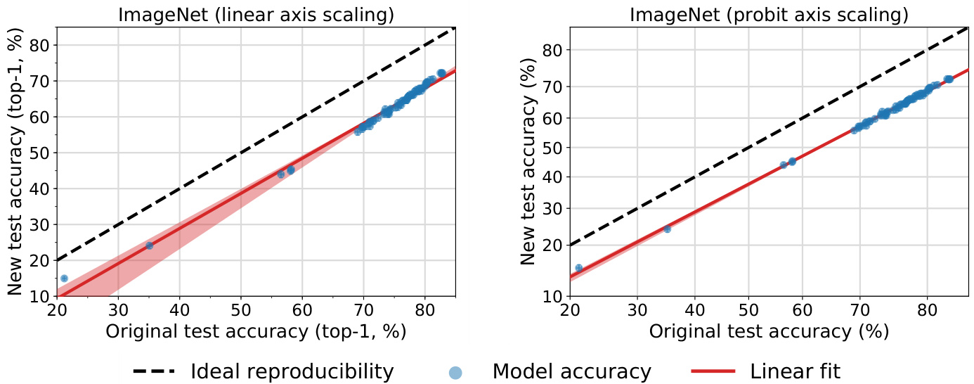
Figure 6: Model accuracy on the original ImageNet validation set vs. our new test set MatchedFrequency. Each data point corresponds to one model in our testbed (shown with $95%$ Clopper-Pearson confidence intervals), and we now also include the Fisher Vector models. The left plot shows the model accuracies with a linear scale on the axes. The right plot instead uses a probit scale, i.e., accuracy $\alpha$ appears at $\Phi^{-1}(\alpha)$ , where $\Phi$ is the Gaussian CDF. Comparing the two plot provides evidence that the probit model is a better fit for the accuracy scores. Over a range of 60 percentage points, the linear fit in the probit domain accurately describes the relationship between original and new test set accuracy. The shaded region around the linear fit is a $95%$ confidence region from 100,000 bootstrap samples. The confidence region is present in both plots but is significantly smaller in the right plot due to the better fit in the probit domain.
图 6: 原始ImageNet验证集与我们的新测试集MatchedFrequency上的模型准确率对比。每个数据点对应测试平台中的一个模型(显示为95% Clopper-Pearson置信区间),本次分析还加入了Fisher Vector模型。左图采用线性坐标轴展示模型准确率,右图则使用概率单位(probit)尺度,即准确率α对应Φ⁻¹(α)位置(Φ表示高斯累积分布函数)。两图对比表明概率单位模型能更好地拟合准确率分数。在60个百分点的范围内,概率单位域的线性拟合精确描述了原始测试集与新测试集准确率的关系。线性拟合周围的阴影区域是通过10万次自助采样(bootstrap)得出的95%置信区间。虽然两图都显示该置信区间,但由于概率单位域的拟合效果更佳,右图中的置信区间明显更小。
C.3 Follow-up Hypotheses
C.3 后续假设
As for CIFAR-10, the gap between original and new accuracy is concerning ly large. Hence we investigated multiple hypotheses for explaining this gap.
至于 CIFAR-10,原始准确率与新准确率之间的差距大得令人担忧。因此我们研究了多种假设来解释这一差距。
C.3.1 Cross Validation
C.3.1 交叉验证
A natural question is whether cross-validation with the existing ImageNet data could have pointed towards a significant drop in accuracy. If adaptive over fitting to the images in the validation set is a cause for the accuracy drop, testing on different images from another cross-validation fold could produce lower accuracies.12 Moreover, recall that the ImageNet validation set is not a strictly i.i.d. sample from the same distribution as the training set (see the beginning of Section 4). This also raises the question of how well a model would perform on a cross-validation fold from the training data.
一个自然的问题是,使用现有的ImageNet数据进行交叉验证是否能预示准确率的显著下降。如果对验证集中图像的适应性过拟合是导致准确率下降的原因,那么在其他交叉验证折的不同图像上进行测试可能会产生更低的准确率。12 此外,回想一下ImageNet验证集并非严格来自与训练集相同分布的独立同分布样本(见第4节开头)。这也引发了另一个问题:模型在训练数据的交叉验证折上表现如何。
To investigate these two effects, we conducted a cross-validation experiment with the ImageNet training and validation sets. In order to ensure that the new cross-validation folds contain only training images, we treated the existing validation set as one fold and created five additional folds with 50,000 images each. To this end, we drew a class-balanced sample of 250,000 images from the training set and then randomly partitioned this sample into five cross-validation folds (again class-balanced). For each of these five folds, we added the validation set (and the other training folds) to the training data so that the size of the training set was unchanged. We then trained one resnet50 model13 [21] for each of the five training sets and evaluated them on the corresponding held-out data. Table 13 shows the resulting accuracies for each split.
为了研究这两种效应,我们在ImageNet训练集和验证集上进行了交叉验证实验。为确保新的交叉验证折仅包含训练图像,我们将现有验证集视为一个折,并创建了五个额外折,每折包含50,000张图像。为此,我们从训练集中抽取了250,000张类别平衡的图像样本,然后将其随机划分为五个类别平衡的交叉验证折。针对这五个折中的每一个,我们将验证集(及其他训练折)加入训练数据,使训练集规模保持不变。随后,我们为每个训练集训练了一个resnet50模型[21],并在对应的保留数据上进行评估。表13展示了各划分的准确率结果。
| Dataset | resnet50 Top-5 Accuracy (%) |
| Original validation set | 92.5 [92.3, 92.8] |
| Split 1 | 92.60 [92.4, 92.8] |
| Split 2 | 92.59 [92.4, 92.8] |
| Split 3 | 92.61 [92.4, 92.8] |
| Split 4 | 92.55 5[92.3, 92.8] |
| Split 5 | 92.62 2[92.4, 92.9] |
| New test set (MatchedFrequency) | 84.7 [83.9, 85.4] |
| 数据集 | ResNet50 Top-5准确率 (%) |
|---|---|
| 原始验证集 | 92.5 [92.3, 92.8] |
| 拆分集1 | 92.60 [92.4, 92.8] |
| 拆分集2 | 92.59 [92.4, 92.8] |
| 拆分集3 | 92.61 [92.4, 92.8] |
| 拆分集4 | 92.55 [92.3, 92.8] |
| 拆分集5 | 92.62 [92.4, 92.9] |
| 新测试集 (MatchedFrequency) | 84.7 [83.9, 85.4] |
Table 13: resnet50 accuracy on cross-validation splits created from the original ImageNet train and validation sets. The accuracy increase is likely caused by a small shift in distribution between the ImageNet training and validation sets.
表 13: 基于原始ImageNet训练集和验证集创建的交叉验证分割中resnet50的准确率。准确率提升可能是由于ImageNet训练集和验证集之间存在微小分布偏移所致。
Overall, we do not see a large difference in accuracy on the new cross validation splits: all differences fall within the $95%$ confidence intervals around the accuracy scores. This is in contrast to the significantly larger accuracy drops on our new test sets.
总体而言,我们在新的交叉验证分割集上未观察到准确率的显著差异:所有差异均落在准确率分数的95%置信区间内。这与新测试集上出现的明显准确率下降形成鲜明对比。
C.3.2 Impact of Dataset Revisions
C.3.2 数据集修订的影响
As mentioned in Section C.1.2, our final reviewing pass may have led to a distribution shift compared to the original ImageNet validation set. In general, our reviewing criterion was to blacklist images that were
如C.1.2节所述,我们的最终审核流程可能导致与原始ImageNet验证集相比出现分布偏移。总体而言,我们的审核标准是将那些
For each class, our reviewing UI (screenshot in Appendix C.4.2) displayed a random sample of ten original validation images directly next to the ten new candidate images currently chosen. At least to some extent, this allowed us to detect and correct distribution shifts between the original validation set and our candidate pool. As a concrete example, we noted in one revision of our dataset that approximately half of the images for “great white shark” were not live sharks in the water but models in museums or statues outside. In contrast, the ImageNet validation set had fewer examples of such artificial sharks. Hence we decided to remove some non-live sharks from our candidate pool and sampled new shark images as a replacement in the dataset.
对于每个类别,我们的审核界面(附录C.4.2中的截图)会在当前选出的十张新候选图像旁随机显示十张原始验证图像。这至少在一定程度上帮助我们检测并修正原始验证集与候选池之间的分布偏移。举例来说,在数据集的一次修订中,我们注意到"大白鲨"类别中约半数图像并非活体鲨鱼,而是博物馆模型或户外雕像。相比之下,ImageNet验证集中这类人工鲨鱼样本较少。因此我们决定从候选池中移除部分非活体鲨鱼图像,并在数据集中采样新的鲨鱼图像作为替代。
Unfortunately, some of these reviewing choices are subjective. However, such choices are often an inherent part of creating a dataset and it is unclear whether a more “hands-off” approach would lead to more meaningful conclusions. For instance, if the drop in accuracy was mainly caused by a distribution shift that is easy to identify and correct (e.g., an increase in black-and-white images), the resulting drop may not be an interesting phenomenon (beyond counting black-and-white images). Hence we decided to both remove distribution shifts that we found easy to identify visually, and also to measure the effect of these interventions.
遗憾的是,这些审查选择中有些是主观的。然而,这类选择往往是创建数据集过程中固有的部分,尚不清楚更"放任"的方法是否能得出更有意义的结论。例如,如果准确率下降主要由易于识别和修正的分布偏移引起(如黑白图像增加),由此产生的下降可能就不是一个有趣的现象(除了统计黑白图像数量之外)。因此我们决定既移除那些通过目视容易识别的分布偏移,同时也测量这些干预措施的效果。
Our reviewing process was iterative, i.e., we made a full pass over every incomplete class in a given dataset revision before sampling new images to fill the resulting gaps. Each time we re-sampled our dataset, we saved the current list of images in our version control system. This allowed us to track the datasets over time and later measure the model accuracy for each dataset revision. We remark that we only computed model accuracies on intermediate revisions after we had arrived at the final revision of the corresponding dataset.
我们的审核过程是迭代式的,即在每次数据集修订中,我们会先对所有不完整的类别进行全面检查,然后再采样新图像填补空缺。每次重新采样数据集时,我们都会将当前图像列表保存到版本控制系统中。这使我们能够跟踪数据集的演变过程,并在后续计算每个数据集修订版本的模型准确率。需要说明的是,我们仅在完成对应数据集的最终修订后,才会计算中间修订版本的模型准确率。
Figure 7 plots the top-1 accuracy of a resnet50 model versus the dataset revision for our new Matched Frequency test set. Overall, reviewing improved model accuracy by about 4% for this dataset. This is evidence that our manual reviewing did not cause the drop in accuracy between the original and new dataset.
图 7: 展示了resnet50模型在我们新构建的Matched Frequency测试集上top-1准确率随数据集修订的变化情况。总体而言,人工审核使该数据集的模型准确率提升了约4%。这表明原始数据集与新数据集之间的准确率下降并非由人工审核导致。
In addition, we also investigated whether the linear relationship between original and new test accuracy was affected by our final reviewing passes. To this end, we evaluated our model testbed on the first revision of our Matched Frequency test set. As can be seen in Figure 8, the resulting accuracies still show a good linear fit that is of similar quality as in Figure 12. This shows that the linear relationship between the test accuracies is not a result of our reviewing intervention.
此外,我们还研究了原始测试准确率与新测试准确率之间的线性关系是否受到最终审核环节的影响。为此,我们在Matched Frequency测试集的首个修订版本上评估了模型测试平台。如图8所示,所得准确率仍呈现良好的线性拟合,其质量与图12相当。这表明测试准确率之间的线性关系并非审核干预的结果。
C.4 Additional Figures, Tables, and Lists
C.4 其他图表和列表
In this appendix we provide large figures etc. that did not fit into the preceding sections about our ImageNet experiments.
在本附录中,我们提供了关于ImageNet实验的大幅图表等内容,这些内容未包含在前述章节中。
C.4.1 MTurk User Interfaces
C.4.1 MTurk用户界面
For comparison, we include the original ImageNet MTurk user interface (UI) in Figure 9 and the MTurk UI we used in our experiments in Figure 10. Each UI corresponds to one task for the MTurk workers, which consists of 48 images in both cases. In contrast to the original ImageNet UI, our UI takes up more than one screen. This requires the MTurk workers to scroll but also provides more details in the images. While the task descriptions are not exactly the same, they are very similar and contain the same directions (e.g., both descriptions ask the MTurk workers to exclude drawings or paintings).
为便于对比,我们在图9中展示了原始ImageNet MTurk用户界面(UI),在图10中呈现了实验所用的MTurk界面。每个UI对应MTurk工作者的一项任务,两种情况下均包含48张图像。与原始ImageNet界面不同,我们的界面需要滚动浏览超过一屏内容,这虽增加了操作步骤,但能呈现更丰富的图像细节。尽管任务描述文字存在细微差异,但核心指引高度一致(例如均要求排除绘画类作品)。
C.4.2 User Interface for our Final Reviewing Process
C.4.2 最终评审流程的用户界面
Figure 11 shows a screenshot of the reviewing UI that the paper authors used to manually review the new ImageNet datasets. At the top, the UI displays the wnid (“n01667114”), the synset (mud turtle), and the gloss. Next, a grid of 20 images is shown in 4 rows.
图 11: 展示了论文作者用于手动审核新版ImageNet数据集的用户界面截图。顶部区域显示了wnid ("n01667114") 、同义词集(mud turtle)和释义。接着以4行网格形式展示了20张图片。
The top two rows correspond to the candidate images currently sampled for the new dataset. Below each image, our UI shows a unique identifier for the image and the date the image was taken. There is also a check box to blacklist any incorrect images. In addition, there is a check box for each image to add it to the blacklist of incorrect images. If an image is added to the blacklist, it will be removed in the next revision of the dataset and replaced with a new image from the candidate pools. The candidate images are sorted by the date they were taken, which makes it easier to spot and remove near-duplicates. Images are marked as near-duplicates by adding their identifier to the “Near-duplicate set” text field.
最上方两行对应当前为新数据集采样的候选图像。每张图片下方,我们的用户界面会显示该图片的唯一标识符和拍摄日期。同时设有复选框可将错误图片加入黑名单。若某张图片被加入黑名单,将在数据集的下个修订版本中被移除,并由候选池中的新图片替代。候选图片按拍摄日期排序,便于识别和移除近似重复项。通过将标识符填入"近似重复集"文本框,即可将图片标记为近似重复项。
The bottom two rows correspond to a random sample of images from the validation set that belong to the target class. We display these images to make it easier to detect and correct for distribution shifts between our new test sets and the original ImageNet validation dataset.
最后两行对应验证集中属于目标类别的随机图像样本。我们展示这些图像是为了更容易检测和纠正新测试集与原始ImageNet验证数据集之间的分布偏移。
C.4.3 Full List of Models Evaluated on ImageNet
C.4.3 在ImageNet上评估的完整模型列表
The following list contains all models we evaluated on ImageNet with references and links to the corresponding source code.
以下列表包含我们在ImageNet上评估的所有模型,并附有参考文献和对应源代码的链接。
C.4.4 Full Results Tables
C.4.4 完整结果表格
Tables 14 and 15 contain the detailed accuracy scores (top-1 and top-5, respectively) for the original ImageNet validation set and our main new test set Matched Frequency. Tables 16 – 19 contain the accuracy scores for our Threshold0.7 and TopImages test sets.
表14和表15分别包含原始ImageNet验证集和我们的主要新测试集Matched Frequency的详细准确率分数(top-1和top-5)。表16至表19包含我们的Threshold0.7和TopImages测试集的准确率分数。

Figure 7: Impact of the reviewing passes on the accuracy of a resnet152 on our new Matched Frequency test set. The revision numbers correspond to the chronological ordering in which we created the dataset revisions
图 7: 审核轮次对resnet152在我们新构建的Matched Frequency测试集上准确率的影响。修订编号对应我们创建数据集修订版本的时间顺序

Figure 8: Model accuracy on the original ImageNet validation set vs. accuracy on the first revision of our Matched Frequency test set. Each data point corresponds to one model in our testbed (shown with $95%$ Clopper-Pearson confidence intervals). The red shaded region is a $95%$ confidence region for the linear fit from 100,000 bootstrap samples. The plots show that the linear relationship between original and new test accuracy also occurs without our final dataset reviewing step. The accuracy plots for the final revision of Matched Frequency can be found in Figure 12.
图 8: 原始ImageNet验证集上的模型准确率与我们匹配频率测试集第一版准确率的对比。每个数据点对应测试平台中的一个模型 (显示为95% Clopper-Pearson置信区间) 。红色阴影区域是通过10万次bootstrap采样得到的线性拟合95%置信区域。图表表明,即使不进行最终数据集审核步骤,原始测试准确率与新测试准确率之间仍存在线性关系。匹配频率最终修订版的准确率图表见图12。

Figure 9: The user interface employed in the original ImageNet collection process for the labeling tasks on Amazon Mechanical Turk.
图 9: 原始ImageNet数据收集过程中在Amazon Mechanical Turk上用于标注任务的用户界面。
This research study is being conducted by Be nR echt,Rebecca Roe l of s,Ludwig Schmidt,and V aisha al Shankar from UC Berkeley.For question about this study, please contact ludwig@berkeley.edu and roelofs@cs.berkeley.edu. In this study,we willask you to indicate whether given image belong to a certain object category.Occasionally,the images may contain disturbing or adult content.Wewould like to remind you that participation in our study is voluntary and that you can withdraw from the study at any time.
本研究由加州大学伯克利分校的Ben Recht、Rebecca Roelofs、Ludwig Schmidt和Vaishaal Shankar共同开展。如有问题请联系ludwig@berkeley.edu与roelofs@cs.berkeley.edu。本研究将要求您判断给定图像是否属于特定物体类别。部分图像可能包含令人不适或成人内容。请注意参与本研究完全自愿,您可随时退出。
Which of these images contain at least one object of type
这些图像中哪些包含至少一个类型为
English foxhound
英国猎狐犬
efinition:an English breed slightly larger than the American foxhounds originally used to hunt in pac
定义:一种英国犬种,体型略大于美国猎狐犬,最初用于狩猎
Task:
任务:
For each of the following images, check the boxnext to an image if it contains at least one object of type English foxhound.Select an image if i contains the object regardless of occlusions,other objects, and clutter or text in the scene.Only select images that are photographs (no drawingsor paintings).
对于以下每张图片,若其中包含至少一只英国猎狐犬(English foxhound)对象,请勾选该图片旁边的方框。无论是否存在遮挡物、其他对象、场景杂乱或文字,只要包含该对象即选择该图片。仅选择照片类图片(不包含绘画或素描作品)。
Please make accurate selections!
请准确选择!
If you are unsure about the object meaning, please also consult the following Wikipedia page(s): https://en.wikipedia.org/wiki/English Foxhound Ifit is impossible to complete a HIT due to missing data or other problems, please return the HIT.
如果不确定对象含义,请查阅以下维基百科页面:https://en.wikipedia.org/wiki/English_Foxhound 若因数据缺失或其他问题无法完成HIT,请退回该HIT。

Figure 10: Our user interface for labeling tasks on Amazon Mechanical Turk. The screenshot here omits the scroll bar and shows only a subset of the entire MTurk task. As in the ImageNet UI, the full task involves a grid of 48 images.
图 10: 我们在Amazon Mechanical Turk上用于标注任务的用户界面。此截图省略了滚动条,仅显示整个MTurk任务的一部分。与ImageNet界面类似,完整任务包含48张图片组成的网格。
n01667114
n01667114
mud turtle
泥龟

bottom-dwelling freshwater turtle inhabiting muddy rivers of North America and Central America Figure 11: The user interface we built to review dataset revisions and remove incorrect or near duplicate images. This user interface was not used for MTurk but only in the final dataset review step conducted by the authors of this paper.
图 11: 我们构建的用户界面,用于审查数据集修订并删除错误或近似重复的图像。该用户界面未用于MTurk,仅用于本文作者进行的最终数据集审查步骤。
Table 14: Top-1 model accuracy on the original ImageNet validation set and our new test set Matched Frequency. $\Delta$ Rank is the relative difference in the ranking from the original test set to the new test set. For example, $\Delta\mathrm{Rank}=-2$ means that a model dropped by two places on the new test set compared to the original test set. The confidence intervals are $95%$ Clopper-Pearson intervals. Due to space constraints, references for the models can be found in Appendix C.4.3. The second part of the table can be found on the following page.
| ImageNet Top-1 MatchedFrequency | |||||||
| Orig. Model | Orig. Accuracy | New Accuracy | New | △ Rank | |||
| Rank | Gap Rank | ||||||
| 1 | pnasnet_large_tf | 82.9 [82.5, 83.2] | 72.2 [71.3, 73.1] | 10.7 10.7 | 3 | -2 | |
| 2 | pnasnet5large | 82.7 [82.4, 83.1] | 72.1 [71.2, 73.0] | 4 | -2 1 | ||
| 3 | nasnet_large_tf | 82.7 [82.4, 83.0] | 72.2 [71.3, 73.1] | 10.5 | 2 | 3 | |
| 4 | nasnetalarge | 82.5 [82.2, 82.8] | 72.2 [71.3, 73.1] | 10.3 10.8 | 1 | ||
| 5 | senet154 | 81.3 [81.0, 81.6] | 70.5 [69.6, 71.4] 70.3 [69.4, 71.2] | 10.5 | 5 | 0 | |
| 6 | polynet | 80.9 [80.5, 81.2] | 6 | 0 | |||
| 7 | inception_resnet_v2_tf | 80.4 [80.0, 80.7] | 69.7 [68.7, 70.6] | 10.7 | 7 | 0 | |
| 8 | inceptionresnetv2 | 80.3 [79.9, 80.6] | 69.6 [68.7, 70.5] | 10.6 | 8 | 0 | |
| 9 | se_resnext101_32x4d | 80.2 [79.9, 80.6] | 69.3 [68.4, 70.2] | 10.9 | 9 | 0 | |
| 10 | inception_v4_tf | 80.2 [79.8, 80.5] | 68.8 [67.9, 69.7] | 11.4 10.9 | 11 | -1 | |
| 11 | inceptionv4 | 80.1 [79.7, 80.4] | 69.1 [68.2, 70.0] | 11.7 | 10 | 1 | |
| 12 | dpn107 | 79.7 [79.4, 80.1] | 68.1 [67.2, 69.0] | 12 | 0 | ||
| 13 | dpn131 | 79.4 [79.1, 79.8] | 67.9 [67.0, 68.8] | 11.5 12.1 | 13 | 0 | |
| 14 | dpn92 | 79.4 [79.0, 79.8] | 67.3 [66.3, 68.2] 67.8 [66.9, 68.8] | 11.4 | 17 | -3 | |
| 15 | dpn98 | 79.2 [78.9, 79.6] | 11.2 | 15 | 0 | ||
| 16 | se_resnext50_32x4d | 79.1 [78.7, 79.4] | 67.9 [66.9, 68.8] | 11.9 | 14 | 2 -3 | |
| 17 | resnext101_64x4d | 79.0 [78.6, 79.3] | 67.1 [66.2, 68.0] | 11.7 | 20 | ||
| 18 | xception | 78.8 [78.5, 79.2] | 67.2 [66.2, 68.1] | 11.1 | 18 | 0 | |
| 19 20 | se_resnet152 | 78.7 [78.3, 79.0] | 67.5 [66.6, 68.5] 67.2 [66.2, 68.1] | 11.2 | 16 19 | 3 1 | |
| 21 | se_resnet101 resnet152 | 78.4 [78.0, 78.8] | 67.0 [66.1, 67.9] | 11.3 | 21 | 0 | |
| 22 | resnext101_32x4d | 78.3 [77.9, 78.7] | 66.2 [65.3, 67.2] | 11.9 | 22 | 0 | |
| 23 | inception_v3_tf | 78.2 [77.8, 78.5] 78.0 [77.6, 78.3] | 66.1 [65.1, 67.0] | 11.9 | 24 | -1 | |
| 24 | resnet_v2_152_tf | 77.8 [77.4, 78.1] | 66.1 [65.1, 67.0] | 11.7 | 25 | -1 | |
| 25 | se_resnet50 | 77.6 [77.3, 78.0] | 66.2 [65.3, 67.2] | 11.4 | 23 | 2 | |
| 26 | fbresnet152 | 77.4 [77.0, 77.8] | 65.8 [64.9, 66.7] | 11.6 26 | 0 | ||
| 27 | resnet101 | 77.4 [77.0, 77.7] | 65.7 [64.7, 66.6] | 11.7 28 | -1 | ||
| 28 | inceptionv3 | 77.3 [77.0, 77.7] | 65.7 [64.8, 66.7] | 11.6 27 | 1 | ||
| 29 | inception_v3 | 77.2 [76.8, 77.6] | 65.4 [64.5, 66.4] | 11.8 29 | 0 | ||
| 30 | densenet161 | 77.1 [76.8, 77.5] | 65.3 [64.4, 66.2] | 11.8 30 | 0 | ||
| 31 | dpn68b | 77.0 [76.7, 77.4] | 64.7 [63.7, 65.6] | 12.4 32 | -1 | ||
| 32 | 77.0 [76.6, 77.3] | 64.6 [63.7, 65.6] | 12.3 34 | -2 | |||
| 33 | resnet_v2_101_tf | 76.9 [76.5, 77.3] | 64.7 [63.7, 65.6] | 12.2 | |||
| densenet201 | 31 | 2 | |||||
表 14: 原始ImageNet验证集与新测试集Matched Frequency上的Top-1模型准确率。$\Delta$ Rank表示从原始测试集到新测试集的排名相对变化。例如,$\Delta\mathrm{Rank}=-2$表示模型在新测试集上的排名比原始测试集下降了两位。置信区间为$95%$ Clopper-Pearson区间。由于篇幅限制,模型参考文献见附录C.4.3。表格第二部分见下页。
| Orig. Rank | Orig. Model | Orig. Accuracy | New Accuracy | New Gap | New Rank | △ Rank |
|---|---|---|---|---|---|---|
| 1 | pnasnet_large_tf | 82.9 [82.5, 83.2] | 72.2 [71.3, 73.1] | 10.7 | 3 | -2 |
| 2 | pnasnet5large | 82.7 [82.4, 83.1] | 72.1 [71.2, 73.0] | 10.6 | 4 | -2 |
| 3 | nasnet_large_tf | 82.7 [82.4, 83.0] | 72.2 [71.3, 73.1] | 10.5 | 2 | 1 |
| 4 | nasnetalarge | 82.5 [82.2, 82.8] | 72.2 [71.3, 73.1] | 10.3 | 1 | 3 |
| 5 | senet154 | 81.3 [81.0, 81.6] | 70.5 [69.6, 71.4] | 10.8 | 5 | 0 |
| 6 | polynet | 80.9 [80.5, 81.2] | 70.3 [69.4, 71.2] | 10.6 | 6 | 0 |
| 7 | inception_resnet_v2_tf | 80.4 [80.0, 80.7] | 69.7 [68.7, 70.6] | 10.7 | 7 | 0 |
| 8 | inceptionresnetv2 | 80.3 [79.9, 80.6] | 69.6 [68.7, 70.5] | 10.7 | 8 | 0 |
| 9 | se_resnext101_32x4d | 80.2 [79.9, 80.6] | 69.3 [68.4, 70.2] | 10.9 | 9 | 0 |
| 10 | inception_v4_tf | 80.2 [79.8, 80.5] | 68.8 [67.9, 69.7] | 11.4 | 11 | -1 |
| 11 | inceptionv4 | 80.1 [79.7, 80.4] | 69.1 [68.2, 70.0] | 11.0 | 10 | 1 |
| 12 | dpn107 | 79.7 [79.4, 80.1] | 68.1 [67.2, 69.0] | 11.6 | 12 | 0 |
| 13 | dpn131 | 79.4 [79.1, 79.8] | 67.9 [67.0, 68.8] | 11.5 | 13 | 0 |
| 14 | dpn92 | 79.4 [79.0, 79.8] | 67.3 [66.3, 68.2] | 12.1 | 17 | -3 |
| 15 | dpn98 | 79.2 [78.9, 79.6] | 67.8 [66.9, 68.8] | 11.4 | 15 | 0 |
| 16 | se_resnext50_32x4d | 79.1 [78.7, 79.4] | 67.9 [66.9, 68.8] | 11.2 | 14 | 2 |
| 17 | resnext101_64x4d | 79.0 [78.6, 79.3] | 67.1 [66.2, 68.0] | 11.9 | 20 | -3 |
| 18 | xception | 78.8 [78.5, 79.2] | 67.2 [66.2, 68.1] | 11.6 | 18 | 0 |
| 19 | se_resnet152 | 78.7 [78.3, 79.0] | 67.5 [66.6, 68.5] | 11.2 | 16 | 3 |
| 20 | se_resnet101 | 78.4 [78.0, 78.8] | 67.2 [66.2, 68.1] | 11.2 | 19 | 1 |
| 21 | resnet152 | 78.4 [78.0, 78.8] | 67.0 [66.1, 67.9] | 11.4 | 21 | 0 |
| 22 | resnext101_32x4d | 78.3 [77.9, 78.7] | 66.2 [65.3, 67.2] | 12.1 | 22 | 0 |
| 23 | inception_v3_tf | 78.2 [77.8, 78.5] | 66.1 [65.1, 67.0] | 12.1 | 24 | -1 |
| 24 | resnet_v2_152_tf | 77.8 [77.4, 78.1] | 66.1 [65.1, 67.0] | 11.7 | 25 | -1 |
| 25 | se_resnet50 | 77.6 [77.3, 78.0] | 66.2 [65.3, 67.2] | 11.4 | 23 | 2 |
| 26 | fbresnet152 | 77.4 [77.0, 77.8] | 65.8 [64.9, 66.7] | 11.6 | 26 | 0 |
| 27 | resnet101 | 77.4 [77.0, 77.7] | 65.7 [64.7, 66.6] | 11.7 | 28 | -1 |
| 28 | inceptionv3 | 77.3 [77.0, 77.7] | 65.7 [64.8, 66.7] | 11.6 | 27 | 1 |
| 29 | inception_v3 | 77.2 [76.8, 77.6] | 65.4 [64.5, 66.4] | 11.8 | 29 | 0 |
| 30 | densenet161 | 77.1 [76.8, 77.5] | 65.3 [64.4, 66.2] | 11.8 | 30 | 0 |
| 31 | dpn68b | 77.0 [76.7, 77.4] | 64.7 [63.7, 65.6] | 12.3 | 32 | -1 |
| 32 | densenet201 | 77.0 [76.6, 77.3] | 64.6 [63.7, 65.6] | 12.4 | 34 | -2 |
| 33 | resnet_v2_101_tf | 76.9 [76.5, 77.3] | 64.7 [63.7, 65.6] | 12.2 | 33 | 0 |
| ImageNet Top-1 MatchedFrequency | |||||||
| Orig. Rank | Model | Orig. Accuracy | New Accuracy | Gap | New Rank | △ Rank | |
| 34 | resnet_v1_152_tf | 76.8 [76.4, 77.2] | 64.6 [63.7, 65.6] | 12.2 | 33 | 1 | |
| 35 | resnet_v1_101_tf | 76.4 [76.0, 76.8] | 64.5 [63.6, 65.5] | 11.9 | 35 | 0 | |
| 36 | cafferesnet101 | 76.2 [75.8, 76.6] | 64.3 [63.4, 65.2] | 11.9 | 36 | 0 | |
| 37 | resnet50 | 76.1 [75.8, 76.5] | 63.3 [62.4, 64.3] | 12.8 | 39 | -2 | |
| 38 | dpn68 | 75.9 [75.5, 76.2] | 63.4 [62.5, 64.4] | 12.4 | 38 | 0 | |
| 39 | densenet169 | 75.6 [75.2, 76.0] | 63.9 [62.9, 64.8] | 11.7 | 37 | 2 | |
| 40 | resnet_v2_50_tf | 75.6 [75.2, 76.0] | 62.7 [61.8, 63.7] | 12.9 | 40 | 0 | |
| 41 | resnet_v1_50_tf | 75.2 [74.8, 75.6] | 62.6 [61.6, 63.5] | 12.6 | 41 | 0 | |
| 42 | densenet121 | 74.4 [74.0, 74.8] | 62.2 [61.3, 63.2] | 12.2 | 42 | 0 | |
| 43 | vgg19_bn | 74.2 [73.8, 74.6] | 61.9 [60.9, 62.8] | 12.3 | 44 | -1 | |
| 44 | pnasnet_mobile_tf | 74.1 [73.8, 74.5] | 60.9 [59.9, 61.8] | 13.3 | 48 | -4 | |
| 45 | nasnetamobile | 74.1 [73.7, 74.5] | 61.6 [60.6, 62.5] | 12.5 | 45 | 0 | |
| 46 | inception_v2_tf | 74.0 [73.6, 74.4] | 61.2 [60.2, 62.2] | 12.8 | 46 | 0 | |
| 47 | nasnet_mobile_tf | 74.0 [73.6, 74.4] | 60.8 [59.8, 61.7] | 13.2 | 50 | -3 | |
| 48 | bninception | 73.5 [73.1, 73.9] | 62.1 [61.2, 63.1] | 11.4 | 43 | 5 | |
| 49 | vgg16_bn | 73.4 [73.0, 73.7] | 60.8 [59.8, 61.7] | 12.6 | 49 | 0 | |
| 50 | resnet34 | 73.3 [72.9, 73.7] | 61.2 [60.2, 62.2] | 12.1 | 47 | 3 | |
| 51 | vgg19 | 72.4 [72.0, 72.8] | 59.7 [58.7, 60.7] | 12.7 | 51 | 0 | |
| 52 | vgg16 | 71.6 [71.2, 72.0] | 58.8 [57.9, 59.8] | 12.8 | 53 | -1 | |
| 53 | vgg13_bn | 71.6 [71.2, 72.0] | 59.0 [58.0, 59.9] | 12.6 | 52 | 1 | |
| 54 | mobilenet_v1_tf | 71.0 [70.6, 71.4] | 57.4 [56.4, 58.4] | 13.6 | 56 | -2 | |
| 55 | vgg_19_tf | 71.0 [70.6, 71.4] | 58.6 [57.7, 59.6] | 12.4 | 54 | 1 | |
| 56 | vgg-16_tf | 70.9 [70.5, 71.3] | 58.4 [57.4, 59.3] | 12.5 | 55 | 1 | |
| 57 | vgg11_bn | 70.4 [70.0, 70.8] | 57.4 [56.4, 58.4] | 13.0 | 57 | 0 | |
| 58 | vgg13 | 69.9 [69.5, 70.3] | 57.1 [56.2, 58.1] | 12.8 | 59 | -1 | |
| 59 | inception_v1_tf | 69.8 [69.4, 70.2] | 56.6 [55.7, 57.6] | 13.1 | 60 | -1 | |
| 60 | resnet18 | 69.8 [69.4, 70.2] | 57.2 [56.2, 58.2] | 12.6 | 58 | 2 | |
| 61 | vgg11 | 69.0 [68.6, 69.4] | 55.8 [54.8, 56.8] | 13.2 | 61 | 0 | |
| 62 | squeezenet1_1 | 58.2 [57.7, 58.6] | 45.3 [44.4, 46.3] | 12.8 62 | 0 | ||
| 63 | squeezenet1_0 | 58.1 [57.7, 58.5] | 45.0 [44.0, 46.0] | 13.1 | 63 | 0 | |
| 64 | alexnet | 56.5 [56.1, 57.0] | 44.0 [43.0, 45.0] | 12.5 64 | 0 | ||
| 65 | fv_64k | 35.1 [34.7, 35.5] | 24.1 [23.2, 24.9] | 11.0 65 | 0 | ||
| 66 | fv_16k | 28.3 [27.9, 28.7] | 19.2 [18.5, 20.0] | 9.1 66 | 0 | ||
| 67 fv_4k | 21.2 [20.8, 21.5] | 15.0 [14.3, 15.7] | 6.2 67 | 0 | |||
| 原始排名 | 模型 | 原始准确率 | 新准确率 | 差距 | 新排名 | 排名变化 |
|---|---|---|---|---|---|---|
| 34 | resnet_v1_152_tf | 76.8 [76.4, 77.2] | 64.6 [63.7, 65.6] | 12.2 | 33 | 1 |
| 35 | resnet_v1_101_tf | 76.4 [76.0, 76.8] | 64.5 [63.6, 65.5] | 11.9 | 35 | 0 |
| 36 | cafferesnet101 | 76.2 [75.8, 76.6] | 64.3 [63.4, 65.2] | 11.9 | 36 | 0 |
| 37 | resnet50 | 76.1 [75.8, 76.5] | 63.3 [62.4, 64.3] | 12.8 | 39 | -2 |
| 38 | dpn68 | 75.9 [75.5, 76.2] | 63.4 [62.5, 64.4] | 12.4 | 38 | 0 |
| 39 | densenet169 | 75.6 [75.2, 76.0] | 63.9 [62.9, 64.8] | 11.7 | 37 | 2 |
| 40 | resnet_v2_50_tf | 75.6 [75.2, 76.0] | 62.7 [61.8, 63.7] | 12.9 | 40 | 0 |
| 41 | resnet_v1_50_tf | 75.2 [74.8, 75.6] | 62.6 [61.6, 63.5] | 12.6 | 41 | 0 |
| 42 | densenet121 | 74.4 [74.0, 74.8] | 62.2 [61.3, 63.2] | 12.2 | 42 | 0 |
| 43 | vgg19_bn | 74.2 [73.8, 74.6] | 61.9 [60.9, 62.8] | 12.3 | 44 | -1 |
| 44 | pnasnet_mobile_tf | 74.1 [73.8, 74.5] | 60.9 [59.9, 61.8] | 13.3 | 48 | -4 |
| 45 | nasnetamobile | 74.1 [73.7, 74.5] | 61.6 [60.6, 62.5] | 12.5 | 45 | 0 |
| 46 | inception_v2_tf | 74.0 [73.6, 74.4] | 61.2 [60.2, 62.2] | 12.8 | 46 | 0 |
| 47 | nasnet_mobile_tf | 74.0 [73.6, 74.4] | 60.8 [59.8, 61.7] | 13.2 | 50 | -3 |
| 48 | bninception | 73.5 [73.1, 73.9] | 62.1 [61.2, 63.1] | 11.4 | 43 | 5 |
| 49 | vgg16_bn | 73.4 [73.0, 73.7] | 60.8 [59.8, 61.7] | 12.6 | 49 | 0 |
| 50 | resnet34 | 73.3 [72.9, 73.7] | 61.2 [60.2, 62.2] | 12.1 | 47 | 3 |
| 51 | vgg19 | 72.4 [72.0, 72.8] | 59.7 [58.7, 60.7] | 12.7 | 51 | 0 |
| 52 | vgg16 | 71.6 [71.2, 72.0] | 58.8 [57.9, 59.8] | 12.8 | 53 | -1 |
| 53 | vgg13_bn | 71.6 [71.2, 72.0] | 59.0 [58.0, 59.9] | 12.6 | 52 | 1 |
| 54 | mobilenet_v1_tf | 71.0 [70.6, 71.4] | 57.4 [56.4, 58.4] | 13.6 | 56 | -2 |
| 55 | vgg_19_tf | 71.0 [70.6, 71.4] | 58.6 [57.7, 59.6] | 12.4 | 54 | 1 |
| 56 | vgg-16_tf | 70.9 [70.5, 71.3] | 58.4 [57.4, 59.3] | 12.5 | 55 | 1 |
| 57 | vgg11_bn | 70.4 [70.0, 70.8] | 57.4 [56.4, 58.4] | 13.0 | 57 | 0 |
| 58 | vgg13 | 69.9 [69.5, 70.3] | 57.1 [56.2, 58.1] | 12.8 | 59 | -1 |
| 59 | inception_v1_tf | 69.8 [69.4, 70.2] | 56.6 [55.7, 57.6] | 13.1 | 60 | -1 |
| 60 | resnet18 | 69.8 [69.4, 70.2] | 57.2 [56.2, 58.2] | 12.6 | 58 | 2 |
| 61 | vgg11 | 69.0 [68.6, 69.4] | 55.8 [54.8, 56.8] | 13.2 | 61 | 0 |
| 62 | squeezenet1_1 | 58.2 [57.7, 58.6] | 45.3 [44.4, 46.3] | 12.8 | 62 | 0 |
| 63 | squeezenet1_0 | 58.1 [57.7, 58.5] | 45.0 [44.0, 46.0] | 13.1 | 63 | 0 |
| 64 | alexnet | 56.5 [56.1, 57.0] | 44.0 [43.0, 45.0] | 12.5 | 64 | 0 |
| 65 | fv_64k | 35.1 [34.7, 35.5] | 24.1 [23.2, 24.9] | 11.0 | 65 | 0 |
| 66 | fv_16k | 28.3 [27.9, 28.7] | 19.2 [18.5, 20.0] | 9.1 | 66 | 0 |
| 67 | fv_4k | 21.2 [20.8, 21.5] | 15.0 [14.3, 15.7] | 6.2 | 67 | 0 |
Table 15: Top-5 model accuracy on the original ImageNet validation set and our new test set Matched Frequency. $\Delta$ Rank is the relative difference in the ranking from the original test set to the new test set. For example, $\Delta\mathrm{Rank}=-2$ means that a model dropped by two places on the new test set compared to the original test set. The confidence intervals are $95%$ Clopper-Pearson intervals. Due to space constraints, references for the models can be found in Appendix C.4.3. The second part of the table can be found on the following page.
| ImageNet Top-5 MatchedFrequency | |||||||
| Orig. Rank | Model | Orig. Accuracy | New Accuracy | Gap | New Rank | △ Rank | |
| 1 | pnasnet_large_tf | 96.2 [96.0, 96.3] | 90.1 [89.5, 90.7] | 6.1 | 3 | -2 | |
| 2 | nasnet_large_tf | 96.2 [96.0, 96.3] | 90.1 [89.5, 90.6] | 6.1 | 4 | -2 | |
| 3 | nasnetalarge | 96.0 [95.8, 96.2] | 90.4 [89.8, 91.0] | 5.6 | 1 | 2 | |
| 4 | pnasnet5large | 96.0 [95.8, 96.2] | 90.2 [89.6, 90.8] | 5.8 | 2 | 2 | |
| 5 | polynet | 95.6 [95.4, 95.7] | 89.1 [88.5, 89.7] | 6.4 | 5 | 0 | |
| 6 | senet154 | 95.5 [95.3, 95.7] | 89.0 [88.4, 89.6] | 6.5 | 6 | 0 | |
| 7 | inception_resnet_v2_tf | 95.2 [95.1, 95.4] | 88.4 [87.7, 89.0] | 6.9 | 9 | -2 | |
| 8 | inception_v4_tf | 95.2 [95.0, 95.4] | 88.3 [87.6, 88.9] | 6.9 | 10 | -2 | |
| 9 | 95.1 [94.9, 95.3] | 88.5 [87.8, 89.1] | 6.7 | 8 | 1 | ||
| 10 | inceptionresnetv2 se_resnext101_32x4d | 95.0 [94.8, 95.2] | 88.0 [87.4, 88.7] | 7.0 | 11 | -1 | |
| 11 | inceptionv4 | 94.9 [94.7, 95.1] | 88.7 [88.1, 89.3] | 6.2 | 7 | 4 | |
| 12 | dpn107 | 94.7 [94.5, 94.9] | 87.6 [86.9, 88.2] | 7.1 | 13 | -1 | |
| 13 | dpn92 | 94.6 [94.4, 94.8] | 87.2 [86.5, 87.8] | 7.5 | 17 | -4 | |
| 14 | dpn131 | 94.6 [94.4, 94.8] | 87.0 [86.3, 87.7] | 7.6 | 19 | -5 | |
| 15 | dpn98 | 94.5 [94.3, 94.7] | 87.2 [86.5, 87.8] | 7.3 | 16 | -1 | |
| 16 | se_resnext50_32x4d | 94.4 [94.2, 94.6] | 87.6 [87.0, 88.3] | 6.8 | 12 | 4 | |
| 17 | se_resnet152 | 94.4 [94.2, 94.6] | 87.4 [86.7, 88.0] | 7.0 | 15 | 2 | |
| 18 | xception | 94.3 [94.1, 94.5] | 87.0 [86.3, 87.7] | 7.3 | 20 | -2 | |
| 19 | se_resnet101 | 94.3 [94.1, 94.5] | 87.1 [86.4, 87.7] | 7.2 | 18 | 1 | |
| 20 | resnext101_64x4d | 94.3 [94.0, 94.5] | 86.9 [86.2, 87.5] | 7.4 | 22 | -2 | |
| 21 | resnet_v2_152_tf | 94.1 [93.9, 94.3] | 86.9 [86.2, 87.5] | 7.2 | 21 | 0 | |
| 22 | resnet152 | 94.0 [93.8, 94.3] | 87.6 [86.9, 88.2] | 6.5 | 14 | 8 | |
| 23 | inception_v3_tf | 93.9 [93.7, 94.1] | 86.4 [85.7, 87.0] | 7.6 | 23 | 0 | |
| 24 | resnext101_32x4d | 93.9 [93.7, 94.1] | 86.2 [85.5, 86.8] | 7.7 | 25 | -1 | |
| 25 | se_resnet50 | 93.8 [93.5, 94.0] | 86.3 [85.6, 87.0] | 7.4 | 24 | 1 | |
| 26 | resnet_v2_101_tf | 93.7 [93.5, 93.9] | 86.1 [85.4, 86.8] | 7.6 | 27 | -1 | |
| 27 | fbresnet152 | 93.6 [93.4, 93.8] | 86.1 [85.4, 86.7] | 7.5 | 28 | -1 | |
| 28 | dpn68b | 93.6 [93.4, 93.8] | 85.3 [84.6, 86.0] | 8.3 | 33 | -5 | |
| 29 | densenet161 | 93.6 [93.3, 93.8] | 86.1 [85.4, 86.8] | 7.4 | 26 | 3 | |
| 30 | resnet101 | 93.5 [93.3, 93.8] | 86.0 [85.3, 86.7] | 7.6 | 30 | 0 | |
| 31 | inception_v3 | 93.5 [93.3, 93.7] | 85.9 [85.2, 86.6] | 7.6 | 31 | 0 | |
| 32 | inceptionv3 | 93.4 [93.2, 93.6] | 86.1 [85.4, 86.7] | 7.4 | 29 | 3 | |
| 93.4 [93.1, 93.6] | 85.3 [84.6, 86.0] | 34 | |||||
| 33 | densenet201 | 8.1 | -1 | ||||
表 15: 原始ImageNet验证集与新测试集Matched Frequency上的Top-5模型准确率。$\Delta$ Rank表示从原始测试集到新测试集的排名相对变化。例如,$\Delta\mathrm{Rank}=-2$表示模型在新测试集上的排名比原始测试集下降了两位。置信区间为$95%$ Clopper-Pearson区间。由于篇幅限制,模型参考文献见附录C.4.3。表格第二部分见下页。
| Orig. Rank | Model | Orig. Accuracy | New Accuracy | Gap | New Rank | △ Rank |
|---|---|---|---|---|---|---|
| 1 | pnasnet_large_tf | 96.2 [96.0, 96.3] | 90.1 [89.5, 90.7] | 6.1 | 3 | -2 |
| 2 | nasnet_large_tf | 96.2 [96.0, 96.3] | 90.1 [89.5, 90.6] | 6.1 | 4 | -2 |
| 3 | nasnetalarge | 96.0 [95.8, 96.2] | 90.4 [89.8, 91.0] | 5.6 | 1 | 2 |
| 4 | pnasnet5large | 96.0 [95.8, 96.2] | 90.2 [89.6, 90.8] | 5.8 | 2 | 2 |
| 5 | polynet | 95.6 [95.4, 95.7] | 89.1 [88.5, 89.7] | 6.4 | 5 | 0 |
| 6 | senet154 | 95.5 [95.3, 95.7] | 89.0 [88.4, 89.6] | 6.5 | 6 | 0 |
| 7 | inception_resnet_v2_tf | 95.2 [95.1, 95.4] | 88.4 [87.7, 89.0] | 6.9 | 9 | -2 |
| 8 | inception_v4_tf | 95.2 [95.0, 95.4] | 88.3 [87.6, 88.9] | 6.9 | 10 | -2 |
| 9 | 95.1 [94.9, 95.3] | 88.5 [87.8, 89.1] | 6.7 | 8 | 1 | |
| 10 | inceptionresnetv2 se_resnext101_32x4d | 95.0 [94.8, 95.2] | 88.0 [87.4, 88.7] | 7.0 | 11 | -1 |
| 11 | inceptionv4 | 94.9 [94.7, 95.1] | 88.7 [88.1, 89.3] | 6.2 | 7 | 4 |
| 12 | dpn107 | 94.7 [94.5, 94.9] | 87.6 [86.9, 88.2] | 7.1 | 13 | -1 |
| 13 | dpn92 | 94.6 [94.4, 94.8] | 87.2 [86.5, 87.8] | 7.5 | 17 | -4 |
| 14 | dpn131 | 94.6 [94.4, 94.8] | 87.0 [86.3, 87.7] | 7.6 | 19 | -5 |
| 15 | dpn98 | 94.5 [94.3, 94.7] | 87.2 [86.5, 87.8] | 7.3 | 16 | -1 |
| 16 | se_resnext50_32x4d | 94.4 [94.2, 94.6] | 87.6 [87.0, 88.3] | 6.8 | 12 | 4 |
| 17 | se_resnet152 | 94.4 [94.2, 94.6] | 87.4 [86.7, 88.0] | 7.0 | 15 | 2 |
| 18 | xception | 94.3 [94.1, 94.5] | 87.0 [86.3, 87.7] | 7.3 | 20 | -2 |
| 19 | se_resnet101 | 94.3 [94.1, 94.5] | 87.1 [86.4, 87.7] | 7.2 | 18 | 1 |
| 20 | resnext101_64x4d | 94.3 [94.0, 94.5] | 86.9 [86.2, 87.5] | 7.4 | 22 | -2 |
| 21 | resnet_v2_152_tf | 94.1 [93.9, 94.3] | 86.9 [86.2, 87.5] | 7.2 | 21 | 0 |
| 22 | resnet152 | 94.0 [93.8, 94.3] | 87.6 [86.9, 88.2] | 6.5 | 14 | 8 |
| 23 | inception_v3_tf | 93.9 [93.7, 94.1] | 86.4 [85.7, 87.0] | 7.6 | 23 | 0 |
| 24 | resnext101_32x4d | 93.9 [93.7, 94.1] | 86.2 [85.5, 86.8] | 7.7 | 25 | -1 |
| 25 | se_resnet50 | 93.8 [93.5, 94.0] | 86.3 [85.6, 87.0] | 7.4 | 24 | 1 |
| 26 | resnet_v2_101_tf | 93.7 [93.5, 93.9] | 86.1 [85.4, 86.8] | 7.6 | 27 | -1 |
| 27 | fbresnet152 | 93.6 [93.4, 93.8] | 86.1 [85.4, 86.7] | 7.5 | 28 | -1 |
| 28 | dpn68b | 93.6 [93.4, 93.8] | 85.3 [84.6, 86.0] | 8.3 | 33 | -5 |
| 29 | densenet161 | 93.6 [93.3, 93.8] | 86.1 [85.4, 86.8] | 7.4 | 26 | 3 |
| 30 | resnet101 | 93.5 [93.3, 93.8] | 86.0 [85.3, 86.7] | 7.6 | 30 | 0 |
| 31 | inception_v3 | 93.5 [93.3, 93.7] | 85.9 [85.2, 86.6] | 7.6 | 31 | 0 |
| 32 | inceptionv3 | 93.4 [93.2, 93.6] | 86.1 [85.4, 86.7] | 7.4 | 29 | 3 |
| 33 | densenet201 | 93.4 [93.1, 93.6] | 85.3 [84.6, 86.0] | 8.1 | 34 | -1 |
| ImageNet Top-5 MatchedFrequency | |||||||
| Orig. Rank | Model | Orig. Accuracy | New Accuracy | Gap | New Rank | △ Rank | |
| 34 | resnet_v1_152_tf | 93.2 [92.9, 93.4] | 85.4 [84.6, 86.0] | 7.8 | 32 | 2 | |
| 35 | resnet_v1_101_tf | 92.9 [92.7, 93.1] | 85.2 [84.5, 85.9] | 7.7 | 35 | 0 | |
| 36 | resnet50 | 92.9 [92.6, 93.1] | 84.7 [83.9, 85.4] | 8.2 | 38 | -2 | |
| 37 | resnet_v2_50_tf | 92.8 [92.6, 93.1] | 84.4 [83.6, 85.1] | 8.5 | 40 | -3 | |
| 38 | densenet169 | 92.8 [92.6, 93.0] | 84.7 [84.0, 85.4] | 8.1 37 | 1 | ||
| 39 | dpn68 | 92.8 [92.5, 93.0] | 84.6 [83.9, 85.3] | 8.2 39 | 0 | ||
| 40 | cafferesnet101 | 92.8 [92.5, 93.0] | 84.9 [84.1, 85.6] | 7.9 36 | 4 | ||
| 41 | resnet_v1_50_tf | 92.2 [92.0, 92.4] | 84.1 [83.4, 84.8] | 8.1 41 | 0 | ||
| 42 | densenet121 | 92.0 [91.7, 92.2] | 83.8 [83.1, 84.5] | 8.2 42 | 0 | ||
| 43 | pnasnet_mobile_tf | 91.9 [91.6, 92.1] | 83.1 [82.4, 83.8] | 8.8 46 | -3 | ||
| 44 | vgg19_bn | 91.8 [91.6, 92.1] | 83.5 [82.7, 84.2] | 8.4 43 | 1 | ||
| 45 | inception_v2_tf | 91.8 [91.5, 92.0] | 83.1 [82.3, 83.8] | 8.7 47 | -2 | ||
| 46 | nasnetamobile | 91.7 [91.5, 92.0] | 83.4 [82.6, 84.1] | 8.4 45 | 1 | ||
| 47 | nasnet_mobile_tf | 91.6 [91.3, 91.8] | 82.2 [81.4, 82.9] | 9.4 50 | -3 | ||
| 48 | bninception | 91.6 [91.3, 91.8] | 83.4 [82.7, 84.2] | 8.1 44 | 4 | ||
| 49 | vgg16_bn | 91.5 [91.3, 91.8] | 83.0 [82.2, 83.7] | 8.6 48 | 1 | ||
| 50 | resnet34 | 91.4 [91.2, 91.7] | 82.7 [82.0, 83.5] | 8.7 49 | 1 | ||
| 51 | vgg19 | 90.9 [90.6, 91.1] | 81.5 [80.7, 82.2] | 9.4 52 | -1 | ||
| 52 | vgg16 | 90.4 [90.1, 90.6] | 81.7 [80.9, 82.4] | 8.7 51 | 1 | ||
| 53 | vgg13_bn | 90.4 [90.1, 90.6] | 81.1 [80.3, 81.9] | 9.3 53 | 0 | ||
| 54 | mobilenet_v1_tf | 90.0 [89.7, 90.2] | 79.4 [78.6, 80.1] | 10.6 60 | -6 | ||
| 56 | vgg_19_tf | 89.8 [89.6, 90.1] | 80.7 [79.9, 81.4] | 9.2 54 | 2 | ||
| 55 | vgg-16_tf | 89.8 [89.6, 90.1] | 80.5 [79.7, 81.3] | 9.3 55 | 0 | ||
| 57 | vgg11_bn | 89.8 [89.5, 90.1] | 80.0 [79.2, 80.8] | 9.8 58 | -1 | ||
| 58 | inception_v1_tf | 89.6 [89.4, 89.9] | 80.1 [79.3, 80.9] | 9.5 57 | 1 | ||
| 59 | vgg13 | 89.2 [89.0, 89.5] | 79.5 [78.7, 80.3] | 9.7 59 | 0 | ||
| 60 | resnet18 | 89.1 [88.8, 89.3] | 80.2 [79.4, 81.0] | 8.9 56 | 4 | ||
| 61 | vgg11 | 88.6 [88.3, 88.9] | 78.8 [78.0, 79.6] | 9.8 61 | 0 | ||
| 62 | squeezenet1_1 | 80.6 [80.3, 81.0] | 69.0 [68.1, 69.9] | 11.6 62 | 0 | ||
| 63 | squeezenet1_0 | 80.4 [80.1, 80.8] | 68.5 [67.6, 69.4] | 11.9 63 | 0 | ||
| 64 | alexnet | 79.1 [78.7, 79.4] | 67.4 [66.5, 68.3] | 11.7 64 | 0 | ||
| 65 | fv_64k | 55.7 [55.3, 56.2] | 42.6 [41.6, 43.6] | 13.2 65 | 0 | ||
| 66 | fv_16k | 49.9 [49.5, 50.4] | 37.5 [36.6, 38.5] | 12.4 66 | 0 | ||
| 67 fv_4k | 41.3 [40.8, 41.7] | 31.0 [30.1, 31.9] | 10.3 67 | 0 | |||
| 原始排名 | 模型 | 原始准确率 | 新准确率 | 差距 | 新排名 | 排名变化 |
|---|---|---|---|---|---|---|
| 34 | resnet_v1_152_tf | 93.2 [92.9, 93.4] | 85.4 [84.6, 86.0] | 7.8 | 32 | 2 |
| 35 | resnet_v1_101_tf | 92.9 [92.7, 93.1] | 85.2 [84.5, 85.9] | 7.7 | 35 | 0 |
| 36 | resnet50 | 92.9 [92.6, 93.1] | 84.7 [83.9, 85.4] | 8.2 | 38 | -2 |
| 37 | resnet_v2_50_tf | 92.8 [92.6, 93.1] | 84.4 [83.6, 85.1] | 8.5 | 40 | -3 |
| 38 | densenet169 | 92.8 [92.6, 93.0] | 84.7 [84.0, 85.4] | 8.1 | 37 | 1 |
| 39 | dpn68 | 92.8 [92.5, 93.0] | 84.6 [83.9, 85.3] | 8.2 | 39 | 0 |
| 40 | cafferesnet101 | 92.8 [92.5, 93.0] | 84.9 [84.1, 85.6] | 7.9 | 36 | 4 |
| 41 | resnet_v1_50_tf | 92.2 [92.0, 92.4] | 84.1 [83.4, 84.8] | 8.1 | 41 | 0 |
| 42 | densenet121 | 92.0 [91.7, 92.2] | 83.8 [83.1, 84.5] | 8.2 | 42 | 0 |
| 43 | pnasnet_mobile_tf | 91.9 [91.6, 92.1] | 83.1 [82.4, 83.8] | 8.8 | 46 | -3 |
| 44 | vgg19_bn | 91.8 [91.6, 92.1] | 83.5 [82.7, 84.2] | 8.4 | 43 | 1 |
| 45 | inception_v2_tf | 91.8 [91.5, 92.0] | 83.1 [82.3, 83.8] | 8.7 | 47 | -2 |
| 46 | nasnetamobile | 91.7 [91.5, 92.0] | 83.4 [82.6, 84.1] | 8.4 | 45 | 1 |
| 47 | nasnet_mobile_tf | 91.6 [91.3, 91.8] | 82.2 [81.4, 82.9] | 9.4 | 50 | -3 |
| 48 | bninception | 91.6 [91.3, 91.8] | 83.4 [82.7, 84.2] | 8.1 | 44 | 4 |
| 49 | vgg16_bn | 91.5 [91.3, 91.8] | 83.0 [82.2, 83.7] | 8.6 | 48 | 1 |
| 50 | resnet34 | 91.4 [91.2, 91.7] | 82.7 [82.0, 83.5] | 8.7 | 49 | 1 |
| 51 | vgg19 | 90.9 [90.6, 91.1] | 81.5 [80.7, 82.2] | 9.4 | 52 | -1 |
| 52 | vgg16 | 90.4 [90.1, 90.6] | 81.7 [80.9, 82.4] | 8.7 | 51 | 1 |
| 53 | vgg13_bn | 90.4 [90.1, 90.6] | 81.1 [80.3, 81.9] | 9.3 | 53 | 0 |
| 54 | mobilenet_v1_tf | 90.0 [89.7, 90.2] | 79.4 [78.6, 80.1] | 10.6 | 60 | -6 |
| 56 | vgg_19_tf | 89.8 [89.6, 90.1] | 80.7 [79.9, 81.4] | 9.2 | 54 | 2 |
| 55 | vgg-16_tf | 89.8 [89.6, 90.1] | 80.5 [79.7, 81.3] | 9.3 | 55 | 0 |
| 57 | vgg11_bn | 89.8 [89.5, 90.1] | 80.0 [79.2, 80.8] | 9.8 | 58 | -1 |
| 58 | inception_v1_tf | 89.6 [89.4, 89.9] | 80.1 [79.3, 80.9] | 9.5 | 57 | 1 |
| 59 | vgg13 | 89.2 [89.0, 89.5] | 79.5 [78.7, 80.3] | 9.7 | 59 | 0 |
| 60 | resnet18 | 89.1 [88.8, 89.3] | 80.2 [79.4, 81.0] | 8.9 | 56 | 4 |
| 61 | vgg11 | 88.6 [88.3, 88.9] | 78.8 [78.0, 79.6] | 9.8 | 61 | 0 |
| 62 | squeezenet1_1 | 80.6 [80.3, 81.0] | 69.0 [68.1, 69.9] | 11.6 | 62 | 0 |
| 63 | squeezenet1_0 | 80.4 [80.1, 80.8] | 68.5 [67.6, 69.4] | 11.9 | 63 | 0 |
| 64 | alexnet | 79.1 [78.7, 79.4] | 67.4 [66.5, 68.3] | 11.7 | 64 | 0 |
| 65 | fv_64k | 55.7 [55.3, 56.2] | 42.6 [41.6, 43.6] | 13.2 | 65 | 0 |
| 66 | fv_16k | 49.9 [49.5, 50.4] | 37.5 [36.6, 38.5] | 12.4 | 66 | 0 |
| 67 | fv_4k | 41.3 [40.8, 41.7] | 31.0 [30.1, 31.9] | 10.3 | 67 | 0 |
Table 16: Top-1 model accuracy on the original ImageNet validation set and our new test set Threshold0.7. $\Delta$ Rank is the relative difference in the ranking from the original test set to the new test set. For example, $\Delta\mathrm{Rank}=-2$ means that a model dropped by two places on the new test set compared to the original test set. The confidence intervals are 95% Clopper-Pearson intervals. Due to space constraints, references for the models can be found in Appendix C.4.3. The second part of the table can be found on the following page.
| ImageNet Top-1 Threshold0.7 | |||||||
| New | |||||||
| Orig. Rank | Model | Orig. Accuracy | New Accuracy | Gap | Rank | △ Rank | |
| 1 | pnasnet_large_tf | 82.9 [82.5, 83.2] | 80.2 [79.4, 80.9] | 2.7 | 2 | -1 | |
| 2 | pnasnet5large | 82.7 [82.4, 83.1] | 80.3 [79.5, 81.1] | 2.4 | 1 | 1 | |
| 3 | nasnet_large_tf | 82.7 [82.4, 83.0] | 80.1 [79.3, 80.9] | 2.6 | 3 | 0 | |
| 4 | nasnetalarge | 82.5 [82.2, 82.8] | 80.0 [79.2, 80.8] | 2.5 | 4 | 0 | |
| 5 | senet154 | 81.3 [81.0, 81.6] | 78.7 [77.8, 79.5] | 2.6 | 5 | 0 | |
| 6 | polynet | 80.9 [80.5, 81.2] | 78.5 [77.7, 79.3] | 2.3 | 6 | 0 | |
| 7 | inception_resnet_v2_tf | 80.4 [80.0, 80.7] | 77.9 [77.1, 78.7] | 2.5 | 8 | -1 | |
| 8 | inceptionresnetv2 | 80.3 [79.9, 80.6] | 78.0 [77.2, 78.8] | 2.3 | 7 | 1 | |
| 9 | se_resnext101_32x4d | 80.2 [79.9, 80.6] | 77.6 [76.8, 78.5] | 2.6 | 11 | -2 | |
| 10 | inception_v4_tf | 80.2 [79.8, 80.5] | 77.8 [77.0, 78.6] | 2.4 | 10 | 0 | |
| 11 | inceptionv4 | 80.1 [79.7, 80.4] | 77.9 [77.0, 78.7] | 2.2 | 9 | 2 | |
| 12 | dpn107 | 79.7 [79.4, 80.1] | 76.6 [75.8, 77.5] | 3.1 | 12 | 0 | |
| 13 | dpn131 | 79.4 [79.1, 79.8] | 76.6 [75.7, 77.4] | 2.9 | 13 | 0 | |
| 14 | dpn92 | 79.4 [79.0, 79.8] | 76.3 [75.5, 77.1] | 3.1 | 17 | -3 | |
| 15 | dpn98 | 79.2 [78.9, 79.6] | 76.3 [75.5, 77.2] | 2.9 | 16 | -1 | |
| 16 | se_resnext50_32x4d | 79.1 [78.7, 79.4] | 76.5 [75.7, 77.3] | 2.6 | 14 | 2 | |
| 17 | resnext101_64x4d | 79.0 [78.6, 79.3] | 75.6 [74.7, 76.4] | 3.4 | 20 | -3 | |
| 18 | xception | 78.8 [78.5, 79.2] | 76.4 [75.5, 77.2] | 2.5 | 15 | 3 | |
| 19 | se_resnet152 | 78.7 [78.3, 79.0] | 76.1 [75.3, 76.9] | 2.5 | 18 | 1 | |
| 20 | se_resnet101 | 78.4 [78.0, 78.8] | 75.8 [75.0, 76.7] | 2.6 | 19 | 1 | |
| 21 | resnet152 | 78.3 [77.9, 78.7] | 75.3 [74.5, 76.2] | 3.0 | 22 | -1 | |
| 22 | resnext101_32x4d | 78.2 [77.8, 78.5] | 75.4 [74.5, 76.2] | 2.8 | 21 | 1 | |
| 23 | inception_v3_tf | 78.0 [77.6, 78.3] | 75.0 [74.2, 75.9] | 2.9 | 24 | -1 | |
| 24 | resnet_v2_152_tf | 77.8 [77.4, 78.1] | 75.2 [74.4, 76.1] | 2.6 | 23 | 1 | |
| 25 | se_resnet50 | 77.6 [77.3, 78.0] | 74.2 [73.3, 75.1] | 3.4 | 30 | -5 | |
| 26 | fbresnet152 | 77.4 [77.0, 77.8] | 74.8 [74.0, 75.7] | 2.6 | 25 | 1 | |
| 27 | resnet101 | 77.4 [77.0, 77.7] | 74.5 [73.6, 75.3] | 2.9 29 | -2 | ||
| 28 | inceptionv3 | 77.3 [77.0, 77.7] | 74.5 [73.6, 75.4] | 2.8 28 | 0 | ||
| 29 | inception_v3 | 77.2 [76.8, 77.6] | 74.7 [73.8, 75.6] | 2.5 26 | 3 | ||
| 30 | densenet161 | 77.1 [76.8, 77.5] | 74.6 [73.7, 75.4] | 2.6 27 | 3 | ||
| 31 | dpn68b | 77.0 [76.7, 77.4] | 73.8 [72.9, 74.7] | 3.2 33 | -2 | ||
| 32 | resnet_v2_101_tf | 77.0 [76.6, 77.3] | 74.0 [73.1, 74.8] | 3.0 31 | 1 | ||
| 33 | densenet201 | 76.9 [76.5, 77.3] | 73.9 [73.1, 74.8] | 3.0 32 | 1 | ||
表 16: 原始ImageNet验证集与新测试集上Top-1模型准确率(Threshold0.7)。$\Delta$ Rank表示从原始测试集到新测试集的排名相对变化。例如,$\Delta\mathrm{Rank}=-2$表示模型在新测试集上的排名比原始测试集下降了两位。置信区间为95% Clopper-Pearson区间。由于篇幅限制,模型参考文献见附录C.4.3。表格第二部分见下页。
| Orig. Rank | Model | Orig. Accuracy | New Accuracy | Gap | Rank | △ Rank |
|---|---|---|---|---|---|---|
| 1 | pnasnet_large_tf | 82.9 [82.5, 83.2] | 80.2 [79.4, 80.9] | 2.7 | 2 | -1 |
| 2 | pnasnet5large | 82.7 [82.4, 83.1] | 80.3 [79.5, 81.1] | 2.4 | 1 | 1 |
| 3 | nasnet_large_tf | 82.7 [82.4, 83.0] | 80.1 [79.3, 80.9] | 2.6 | 3 | 0 |
| 4 | nasnetalarge | 82.5 [82.2, 82.8] | 80.0 [79.2, 80.8] | 2.5 | 4 | 0 |
| 5 | senet154 | 81.3 [81.0, 81.6] | 78.7 [77.8, 79.5] | 2.6 | 5 | 0 |
| 6 | polynet | 80.9 [80.5, 81.2] | 78.5 [77.7, 79.3] | 2.3 | 6 | 0 |
| 7 | inception_resnet_v2_tf | 80.4 [80.0, 80.7] | 77.9 [77.1, 78.7] | 2.5 | 8 | -1 |
| 8 | inceptionresnetv2 | 80.3 [79.9, 80.6] | 78.0 [77.2, 78.8] | 2.3 | 7 | 1 |
| 9 | se_resnext101_32x4d | 80.2 [79.9, 80.6] | 77.6 [76.8, 78.5] | 2.6 | 11 | -2 |
| 10 | inception_v4_tf | 80.2 [79.8, 80.5] | 77.8 [77.0, 78.6] | 2.4 | 10 | 0 |
| 11 | inceptionv4 | 80.1 [79.7, 80.4] | 77.9 [77.0, 78.7] | 2.2 | 9 | 2 |
| 12 | dpn107 | 79.7 [79.4, 80.1] | 76.6 [75.8, 77.5] | 3.1 | 12 | 0 |
| 13 | dpn131 | 79.4 [79.1, 79.8] | 76.6 [75.7, 77.4] | 2.9 | 13 | 0 |
| 14 | dpn92 | 79.4 [79.0, 79.8] | 76.3 [75.5, 77.1] | 3.1 | 17 | -3 |
| 15 | dpn98 | 79.2 [78.9, 79.6] | 76.3 [75.5, 77.2] | 2.9 | 16 | -1 |
| 16 | se_resnext50_32x4d | 79.1 [78.7, 79.4] | 76.5 [75.7, 77.3] | 2.6 | 14 | 2 |
| 17 | resnext101_64x4d | 79.0 [78.6, 79.3] | 75.6 [74.7, 76.4] | 3.4 | 20 | -3 |
| 18 | xception | 78.8 [78.5, 79.2] | 76.4 [75.5, 77.2] | 2.5 | 15 | 3 |
| 19 | se_resnet152 | 78.7 [78.3, 79.0] | 76.1 [75.3, 76.9] | 2.5 | 18 | 1 |
| 20 | se_resnet101 | 78.4 [78.0, 78.8] | 75.8 [75.0, 76.7] | 2.6 | 19 | 1 |
| 21 | resnet152 | 78.3 [77.9, 78.7] | 75.3 [74.5, 76.2] | 3.0 | 22 | -1 |
| 22 | resnext101_32x4d | 78.2 [77.8, 78.5] | 75.4 [74.5, 76.2] | 2.8 | 21 | 1 |
| 23 | inception_v3_tf | 78.0 [77.6, 78.3] | 75.0 [74.2, 75.9] | 2.9 | 24 | -1 |
| 24 | resnet_v2_152_tf | 77.8 [77.4, 78.1] | 75.2 [74.4, 76.1] | 2.6 | 23 | 1 |
| 25 | se_resnet50 | 77.6 [77.3, 78.0] | 74.2 [73.3, 75.1] | 3.4 | 30 | -5 |
| 26 | fbresnet152 | 77.4 [77.0, 77.8] | 74.8 [74.0, 75.7] | 2.6 | 25 | 1 |
| 27 | resnet101 | 77.4 [77.0, 77.7] | 74.5 [73.6, 75.3] | 2.9 | 29 | -2 |
| 28 | inceptionv3 | 77.3 [77.0, 77.7] | 74.5 [73.6, 75.4] | 2.8 | 28 | 0 |
| 29 | inception_v3 | 77.2 [76.8, 77.6] | 74.7 [73.8, 75.6] | 2.5 | 26 | 3 |
| 30 | densenet161 | 77.1 [76.8, 77.5] | 74.6 [73.7, 75.4] | 2.6 | 27 | 3 |
| 31 | dpn68b | 77.0 [76.7, 77.4] | 73.8 [72.9, 74.7] | 3.2 | 33 | -2 |
| 32 | resnet_v2_101_tf | 77.0 [76.6, 77.3] | 74.0 [73.1, 74.8] | 3.0 | 31 | 1 |
| 33 | densenet201 | 76.9 [76.5, 77.3] | 73.9 [73.1, 74.8] | 3.0 | 32 | 1 |
| ImageNet Top-1 Threshold0.7 | ||||||||
| Orig. | ||||||||
| Rank | Model | Orig. Accuracy | New Accuracy | Gap | New Rank | △ Rank | ||
| 34 | resnet_v1_152_tf | 76.8 [76.4, 77.2] | 73.7 [72.9, 74.6] | 3.1 | 34 | 0 | ||
| 35 | resnet_v1_101_tf | 76.4 [76.0, 76.8] | 73.4 [72.5, 74.2] | 3.0 | 35 | 0 | ||
| 36 | cafferesnet101 | 76.2 [75.8, 76.6] | 72.9 [72.0, 73.7] | 3.3 | 37 | -1 | ||
| 37 | resnet50 | 76.1 [75.8, 76.5] | 72.7 [71.8, 73.6] | 3.4 | 38 | -1 | ||
| 38 | dpn68 | 75.9 [75.5, 76.2] | 73.0 [72.1, 73.8] | 2.9 | 36 | 2 | ||
| 39 | densenet169 | 75.6 [75.2, 76.0] | 72.3 [71.4, 73.1] | 3.3 | 40 | -1 | ||
| 40 | resnet_v2_50_tf | 75.6 [75.2, 76.0] | 72.3 [71.4, 73.2] | 3.3 | 39 | 1 | ||
| 41 | resnet_v1_50_tf | 75.2 [74.8, 75.6] | 71.9 [71.0, 72.8] | 3.3 | 41 | 0 | ||
| 42 | densenet121 | 74.4 [74.0, 74.8] | 70.5 [69.6, 71.4] | 3.9 | 47 | -5 | ||
| 43 | vgg19_bn | 74.2 [73.8, 74.6] | 71.4 [70.5, 72.3] | 2.8 | 42 | 1 | ||
| 44 | pnasnet_mobile_tf | 74.1 [73.8, 74.5] | 70.6 [69.7, 71.5] | 3.6 | 46 | -2 | ||
| 45 | nasnetamobile | 74.1 [73.7, 74.5] | 70.9 [70.0, 71.8] | 3.2 | 45 | 0 | ||
| 46 | inception_v2_tf | 74.0 [73.6, 74.4] | 71.1 [70.2, 72.0] | 2.9 | 44 | 2 | ||
| 47 | nasnet_mobile_tf | 74.0 [73.6, 74.4] | 70.0 [69.0, 70.8] | 4.0 | 50 | -3 | ||
| 48 | bninception | 73.5 [73.1, 73.9] | 71.3 [70.4, 72.2] | 2.2 | 43 | 5 | ||
| 49 | vgg16_bn | 73.4 [73.0, 73.7] | 70.2 [69.3, 71.1] | 3.1 | 48 | 1 | ||
| 50 | resnet34 | 73.3 [72.9, 73.7] | 70.2 [69.2, 71.0] | 3.2 | 49 | 1 | ||
| 51 | vgg19 | 72.4 [72.0, 72.8] | 68.7 [67.8, 69.6] | 3.7 | 51 | 0 | ||
| 52 | vgg16 | 71.6 [71.2, 72.0] | 68.0 [67.0, 68.9] | 3.6 | 52 | 0 | ||
| 53 | vgg13_bn | 71.6 [71.2, 72.0] | 67.3 [66.4, 68.2] | 4.3 | 55 | -2 | ||
| 54 | mobilenet_v1_tf | 71.0 [70.6, 71.4] | 66.1 [65.2, 67.0] | 4.9 | 59 | -5 | ||
| 55 | vgg_19_tf | 71.0 [70.6, 71.4] | 67.4 [66.5, 68.3] | 3.6 | 54 | 1 | ||
| 56 | vgg-16_tf | 70.9 [70.5, 71.3] | 67.6 [66.7, 68.5] | 3.3 | 53 | 3 | ||
| 57 | vgg11_bn | 70.4 [70.0, 70.8] | 66.4 [65.5, 67.3] | 4.0 | 58 | -1 | ||
| 58 | vgg13 | 69.9 [69.5, 70.3] | 66.0 [65.0, 66.9] | 4.0 | 60 | -2 | ||
| 59 | inception_v1_tf | 69.8 [69.4, 70.2] | 66.4 [65.5, 67.4] | 3.3 | 57 | 2 | ||
| 60 | resnet18 | 69.8 [69.4, 70.2] | 66.6 [65.7, 67.5] | 3.2 | 56 | 4 | ||
| 61 | vgg11 | 69.0 [68.6, 69.4] | 64.6 [63.7, 65.6] | 4.4 | 61 | 0 | ||
| 62 | squeezenet1_1 | 58.2 [57.7, 58.6] | 54.4 [53.4, 55.4] | 3.8 | 62 | 0 | ||
| 63 | squeezenet1_0 | 58.1 [57.7, 58.5] | 53.4 [52.4, 54.4] | 4.7 | 63 | 0 | ||
| 64 | alexnet | 56.5 [56.1, 57.0] | 51.3 [50.3, 52.3] | 5.2 | 64 | 0 | ||
| 65 | fv_64k | 35.1 [34.7, 35.5] | 29.1 [28.2, 30.0] | 6.0 65 | 0 | |||
| 66 | fv_16k | 28.3 [27.9, 28.7] | 23.4 [22.5, 24.2] | 5.0 | 66 | 0 | ||
| 67 fv_4k | 21.2 [20.8, 21.5] | 17.8 [17.0, 18.5] | 3.4 | 67 | 0 | |||
| 排名 | 模型 | 原始准确率 | 新准确率 | 差距 | 新排名 | 排名变化 |
|---|---|---|---|---|---|---|
| 34 | resnet_v1_152_tf | 76.8 [76.4, 77.2] | 73.7 [72.9, 74.6] | 3.1 | 34 | 0 |
| 35 | resnet_v1_101_tf | 76.4 [76.0, 76.8] | 73.4 [72.5, 74.2] | 3.0 | 35 | 0 |
| 36 | cafferesnet101 | 76.2 [75.8, 76.6] | 72.9 [72.0, 73.7] | 3.3 | 37 | -1 |
| 37 | resnet50 | 76.1 [75.8, 76.5] | 72.7 [71.8, 73.6] | 3.4 | 38 | -1 |
| 38 | dpn68 | 75.9 [75.5, 76.2] | 73.0 [72.1, 73.8] | 2.9 | 36 | 2 |
| 39 | densenet169 | 75.6 [75.2, 76.0] | 72.3 [71.4, 73.1] | 3.3 | 40 | -1 |
| 40 | resnet_v2_50_tf | 75.6 [75.2, 76.0] | 72.3 [71.4, 73.2] | 3.3 | 39 | 1 |
| 41 | resnet_v1_50_tf | 75.2 [74.8, 75.6] | 71.9 [71.0, 72.8] | 3.3 | 41 | 0 |
| 42 | densenet121 | 74.4 [74.0, 74.8] | 70.5 [69.6, 71.4] | 3.9 | 47 | -5 |
| 43 | vgg19_bn | 74.2 [73.8, 74.6] | 71.4 [70.5, 72.3] | 2.8 | 42 | 1 |
| 44 | pnasnet_mobile_tf | 74.1 [73.8, 74.5] | 70.6 [69.7, 71.5] | 3.6 | 46 | -2 |
| 45 | nasnetamobile | 74.1 [73.7, 74.5] | 70.9 [70.0, 71.8] | 3.2 | 45 | 0 |
| 46 | inception_v2_tf | 74.0 [73.6, 74.4] | 71.1 [70.2, 72.0] | 2.9 | 44 | 2 |
| 47 | nasnet_mobile_tf | 74.0 [73.6, 74.4] | 70.0 [69.0, 70.8] | 4.0 | 50 | -3 |
| 48 | bninception | 73.5 [73.1, 73.9] | 71.3 [70.4, 72.2] | 2.2 | 43 | 5 |
| 49 | vgg16_bn | 73.4 [73.0, 73.7] | 70.2 [69.3, 71.1] | 3.1 | 48 | 1 |
| 50 | resnet34 | 73.3 [72.9, 73.7] | 70.2 [69.2, 71.0] | 3.2 | 49 | 1 |
| 51 | vgg19 | 72.4 [72.0, 72.8] | 68.7 [67.8, 69.6] | 3.7 | 51 | 0 |
| 52 | vgg16 | 71.6 [71.2, 72.0] | 68.0 [67.0, 68.9] | 3.6 | 52 | 0 |
| 53 | vgg13_bn | 71.6 [71.2, 72.0] | 67.3 [66.4, 68.2] | 4.3 | 55 | -2 |
| 54 | mobilenet_v1_tf | 71.0 [70.6, 71.4] | 66.1 [65.2, 67.0] | 4.9 | 59 | -5 |
| 55 | vgg_19_tf | 71.0 [70.6, 71.4] | 67.4 [66.5, 68.3] | 3.6 | 54 | 1 |
| 56 | vgg-16_tf | 70.9 [70.5, 71.3] | 67.6 [66.7, 68.5] | 3.3 | 53 | 3 |
| 57 | vgg11_bn | 70.4 [70.0, 70.8] | 66.4 [65.5, 67.3] | 4.0 | 58 | -1 |
| 58 | vgg13 | 69.9 [69.5, 70.3] | 66.0 [65.0, 66.9] | 4.0 | 60 | -2 |
| 59 | inception_v1_tf | 69.8 [69.4, 70.2] | 66.4 [65.5, 67.4] | 3.3 | 57 | 2 |
| 60 | resnet18 | 69.8 [69.4, 70.2] | 66.6 [65.7, 67.5] | 3.2 | 56 | 4 |
| 61 | vgg11 | 69.0 [68.6, 69.4] | 64.6 [63.7, 65.6] | 4.4 | 61 | 0 |
| 62 | squeezenet1_1 | 58.2 [57.7, 58.6] | 54.4 [53.4, 55.4] | 3.8 | 62 | 0 |
| 63 | squeezenet1_0 | 58.1 [57.7, 58.5] | 53.4 [52.4, 54.4] | 4.7 | 63 | 0 |
| 64 | alexnet | 56.5 [56.1, 57.0] | 51.3 [50.3, 52.3] | 5.2 | 64 | 0 |
| 65 | fv_64k | 35.1 [34.7, 35.5] | 29.1 [28.2, 30.0] | 6.0 | 65 | 0 |
| 66 | fv_16k | 28.3 [27.9, 28.7] | 23.4 [22.5, 24.2] | 5.0 | 66 | 0 |
| 67 | fv_4k | 21.2 [20.8, 21.5] | 17.8 [17.0, 18.5] | 3.4 | 67 | 0 |
Table 17: Top-5 model accuracy on the original ImageNet validation set and our new test set Threshold0.7. $\Delta$ Rank is the relative difference in the ranking from the original test set to the new test set. For example, $\Delta\mathrm{Rank}=-2$ means that a model dropped by two places on the new test set compared to the original test set. The confidence intervals are 95% Clopper-Pearson intervals. Due to space constraints, references for the models can be found in Appendix C.4.3. The second part of the table can be found on the following page.
| ImageNet Top-5 Threshold0.7 | New | ||||||
| Orig. Rank | Model | Orig. Accuracy | New Accuracy | Gap | Rank | △ Rank | |
| 1 | pnasnet_large_tf | 96.2 [96.0, 96.3] | 95.6 [95.2, 96.0] | 0.6 | 2 | -1 | |
| 2 | nasnet_large_tf | 96.2 [96.0, 96.3] | 95.7 [95.2, 96.0] | 0.5 | 1 | 1 | |
| 3 | nasnetalarge | 96.0 [95.8, 96.2] | 95.3 [94.9, 95.8] | 0.7 | 4 | -1 | |
| 4 | pnasnet5large | 96.0 [95.8, 96.2] | 95.5 [95.0, 95.9] | 0.5 | 3 | 1 | |
| 5 | polynet | 95.6 [95.4, 95.7] | 94.9 [94.4, 95.3] | 0.7 | 5 | 0 | |
| 6 | senet154 | 95.5 [95.3, 95.7] | 94.8 [94.3, 95.2] | 0.7 | 6 | 0 | |
| 7 | inception_resnet_v2_tf | 95.2 [95.1, 95.4] | 94.7 [94.2, 95.1] | 0.6 | 7 | 0 | |
| 8 | inception_v4_tf | 95.2 [95.0, 95.4] | 94.4 [94.0, 94.9] | 0.8 | 9 | -1 | |
| 9 | inceptionresnetv2 | 95.1 [94.9, 95.3] | 94.5 [94.1, 95.0] | 0.6 | 8 | 1 | |
| 10 | se_resnext101_32x4d | 95.0 [94.8, 95.2] | 94.3 [93.8, 94.7] | 0.7 | 11 | -1 | |
| 11 | inceptionv4 | 94.9 [94.7, 95.1] | 94.3 [93.8, 94.7] | 0.6 | 10 | 1 | |
| 12 | dpn107 | 94.7 [94.5, 94.9] | 93.7 [93.2, 94.2] | 1.0 | 12 | 0 | |
| 13 | dpn92 | 94.6 [94.4, 94.8] | 93.7 [93.2, 94.2] | 0.9 | 14 | -1 | |
| 14 | dpn131 | 94.6 [94.4, 94.8] | 93.5 [92.9, 93.9] | 1.1 | 20 | -6 | |
| 15 | dpn98 | 94.5 [94.3, 94.7] | 93.6 [93.1, 94.1] | 0.9 | 17 | -2 | |
| 16 | se_resnext50_32x4d | 94.4 [94.2, 94.6] | 93.6 [93.1, 94.1] | 0.8 | 16 | 0 | |
| 17 | se_resnet152 | 94.4 [94.2, 94.6] | 93.7 [93.2, 94.2] | 0.7 | 13 | 4 | |
| 18 | xception | 94.3 [94.1, 94.5] | 93.6 [93.1, 94.1] | 0.7 | 18 | 0 | |
| 19 | se_resnet101 | 94.3 [94.1, 94.5] | 93.6 [93.1, 94.0] | 0.7 | 19 | 0 | |
| 20 | resnext101_64x4d | 94.3 [94.0, 94.5] | 93.3 [92.8, 93.8] | 0.9 | 22 | -2 | |
| 21 | resnet_v2_152_tf | 94.1 [93.9, 94.3] | 93.4 [92.9, 93.9] | 0.7 | 21 | 0 | |
| 22 | resnet152 | 94.0 [93.8, 94.3] | 93.7 [93.2, 94.2] | 0.4 | 15 | 7 | |
| 23 | inception_v3_tf | 93.9 [93.7, 94.1] | 92.8 [92.3, 93.3] | 1.1 | 25 | -2 | |
| 24 | resnext101_32x4d | 93.9 [93.7, 94.1] | 92.7 [92.2, 93.2] | 1.2 | 28 | -4 | |
| 25 | se_resnet50 | 93.8 [93.5, 94.0] | 93.0 [92.4, 93.5] | 0.8 | 24 | 1 | |
| 26 | resnet_v2_101_tf | 93.7 [93.5, 93.9] | 93.2 [92.7, 93.7] | 0.5 | 23 | 3 | |
| 27 | fbresnet152 | 93.6 [93.4, 93.8] | 92.7 [92.1, 93.2] | 0.9 | 29 | -2 | |
| 28 | dpn68b | 93.6 [93.4, 93.8] | 92.7 [92.1, 93.2] | 0.9 | 31 | -3 | |
| 29 | densenet161 | 93.6 [93.3, 93.8] | 92.8 [92.3, 93.3] | 0.8 | 26 | 3 | |
| 30 | resnet101 | 93.5 [93.3, 93.8] | 92.8 [92.3, 93.3] | 0.8 | 27 | 3 | |
| 31 | inception_v3 | 93.5 [93.3, 93.7] | 92.7 [92.1, 93.2] | 0.9 30 | 1 | ||
| 32 | inceptionv3 | 93.4 [93.2, 93.6] | 92.6 [92.1, 93.1] | 0.8 32 | 0 | ||
| 33 | densenet201 | 93.4 [93.1, 93.6] | 92.4 [91.9, 92.9] | 33 | 0 | ||
| 1.0 | |||||||
表 17: 原始ImageNet验证集与新测试集上Top-5模型准确率对比(阈值0.7)。$\Delta$ Rank表示从原始测试集到新测试集的排名相对变化。例如,$\Delta\mathrm{Rank}=-2$表示模型在新测试集上的排名比原始测试集下降了两位。置信区间为95% Clopper-Pearson区间。由于篇幅限制,模型参考文献见附录C.4.3。表格第二部分见下页。
| Orig. Rank | Model | Orig. Accuracy | New Accuracy | Gap | Rank | △ Rank |
|---|---|---|---|---|---|---|
| 1 | pnasnet_large_tf | 96.2 [96.0, 96.3] | 95.6 [95.2, 96.0] | 0.6 | 2 | -1 |
| 2 | nasnet_large_tf | 96.2 [96.0, 96.3] | 95.7 [95.2, 96.0] | 0.5 | 1 | 1 |
| 3 | nasnetalarge | 96.0 [95.8, 96.2] | 95.3 [94.9, 95.8] | 0.7 | 4 | -1 |
| 4 | pnasnet5large | 96.0 [95.8, 96.2] | 95.5 [95.0, 95.9] | 0.5 | 3 | 1 |
| 5 | polynet | 95.6 [95.4, 95.7] | 94.9 [94.4, 95.3] | 0.7 | 5 | 0 |
| 6 | senet154 | 95.5 [95.3, 95.7] | 94.8 [94.3, 95.2] | 0.7 | 6 | 0 |
| 7 | inception_resnet_v2_tf | 95.2 [95.1, 95.4] | 94.7 [94.2, 95.1] | 0.6 | 7 | 0 |
| 8 | inception_v4_tf | 95.2 [95.0, 95.4] | 94.4 [94.0, 94.9] | 0.8 | 9 | -1 |
| 9 | inceptionresnetv2 | 95.1 [94.9, 95.3] | 94.5 [94.1, 95.0] | 0.6 | 8 | 1 |
| 10 | se_resnext101_32x4d | 95.0 [94.8, 95.2] | 94.3 [93.8, 94.7] | 0.7 | 11 | -1 |
| 11 | inceptionv4 | 94.9 [94.7, 95.1] | 94.3 [93.8, 94.7] | 0.6 | 10 | 1 |
| 12 | dpn107 | 94.7 [94.5, 94.9] | 93.7 [93.2, 94.2] | 1.0 | 12 | 0 |
| 13 | dpn92 | 94.6 [94.4, 94.8] | 93.7 [93.2, 94.2] | 0.9 | 14 | -1 |
| 14 | dpn131 | 94.6 [94.4, 94.8] | 93.5 [92.9, 93.9] | 1.1 | 20 | -6 |
| 15 | dpn98 | 94.5 [94.3, 94.7] | 93.6 [93.1, 94.1] | 0.9 | 17 | -2 |
| 16 | se_resnext50_32x4d | 94.4 [94.2, 94.6] | 93.6 [93.1, 94.1] | 0.8 | 16 | 0 |
| 17 | se_resnet152 | 94.4 [94.2, 94.6] | 93.7 [93.2, 94.2] | 0.7 | 13 | 4 |
| 18 | xception | 94.3 [94.1, 94.5] | 93.6 [93.1, 94.1] | 0.7 | 18 | 0 |
| 19 | se_resnet101 | 94.3 [94.1, 94.5] | 93.6 [93.1, 94.0] | 0.7 | 19 | 0 |
| 20 | resnext101_64x4d | 94.3 [94.0, 94.5] | 93.3 [92.8, 93.8] | 0.9 | 22 | -2 |
| 21 | resnet_v2_152_tf | 94.1 [93.9, 94.3] | 93.4 [92.9, 93.9] | 0.7 | 21 | 0 |
| 22 | resnet152 | 94.0 [93.8, 94.3] | 93.7 [93.2, 94.2] | 0.4 | 15 | 7 |
| 23 | inception_v3_tf | 93.9 [93.7, 94.1] | 92.8 [92.3, 93.3] | 1.1 | 25 | -2 |
| 24 | resnext101_32x4d | 93.9 [93.7, 94.1] | 92.7 [92.2, 93.2] | 1.2 | 28 | -4 |
| 25 | se_resnet50 | 93.8 [93.5, 94.0] | 93.0 [92.4, 93.5] | 0.8 | 24 | 1 |
| 26 | resnet_v2_101_tf | 93.7 [93.5, 93.9] | 93.2 [92.7, 93.7] | 0.5 | 23 | 3 |
| 27 | fbresnet152 | 93.6 [93.4, 93.8] | 92.7 [92.1, 93.2] | 0.9 | 29 | -2 |
| 28 | dpn68b | 93.6 [93.4, 93.8] | 92.7 [92.1, 93.2] | 0.9 | 31 | -3 |
| 29 | densenet161 | 93.6 [93.3, 93.8] | 92.8 [92.3, 93.3] | 0.8 | 26 | 3 |
| 30 | resnet101 | 93.5 [93.3, 93.8] | 92.8 [92.3, 93.3] | 0.8 | 27 | 3 |
| 31 | inception_v3 | 93.5 [93.3, 93.7] | 92.7 [92.1, 93.2] | 0.9 | 30 | 1 |
| 32 | inceptionv3 | 93.4 [93.2, 93.6] | 92.6 [92.1, 93.1] | 0.8 | 32 | 0 |
| 33 | densenet201 | 93.4 [93.1, 93.6] | 92.4 [91.9, 92.9] | 1.0 | 33 | 0 |
| ImageNet Top-5 Threshold0.7 | |||||||
| Orig. Rank Model | New | ||||||
| Orig. Accuracy | New Accuracy | Gap | Rank | △ Rank | |||
| 34 | resnet_v1_152_tf | 93.2 [92.9, 93.4] | 92.2 [91.7, 92.7] | 1.0 34 | 0 | ||
| 35 | resnet_v1_101_tf | 92.9 [92.7, 93.1] | 92.0 [91.5, 92.5] | 0.9 | 36 | -1 | |
| 36 | resnet50 | 92.9 [92.6, 93.1] | 92.0 [91.5, 92.5] | 0.9 | 37 | -1 | |
| 37 | resnet_v2_50_tf | 92.8 [92.6, 93.1] | 91.9 [91.4, 92.5] | 0.9 | 38 | -1 | |
| 38 | densenet169 | 92.8 [92.6, 93.0] | 91.9 [91.4, 92.4] | 0.9 | 39 | -1 | |
| 39 | dpn68 | 92.8 [92.5, 93.0] | 92.1 [91.5, 92.6] | 0.7 | 35 | 4 | |
| 40 | cafferesnet101 | 92.8 [92.5, 93.0] | 91.6 [91.1, 92.2] | 1.1 | 40 | 0 | |
| 41 | resnet_v1_50_tf | 92.2 [92.0, 92.4] | 91.1 [90.6, 91.7] | 1.0 | 41 | 0 | |
| 42 | densenet121 | 92.0 [91.7, 92.2] | 91.1 [90.5, 91.6] | 0.9 | 42 | 0 | |
| 43 | pnasnet_mobile_tf | 91.9 [91.6, 92.1] | 90.7 [90.1, 91.3] | 1.1 47 | -4 | ||
| 44 | vgg19_bn | 91.8 [91.6, 92.1] | 91.0 [90.4, 91.5] | 0.9 44 | 0 | ||
| 45 | inception_v2_tf | 91.8 [91.5, 92.0] | 91.0 [90.5, 91.6] | 0.7 43 | 2 | ||
| 46 | nasnetamobile | 91.7 [91.5, 92.0] | 90.9 [90.3, 91.4] | 0.9 46 | 0 | ||
| 47 | nasnet_mobile_tf | 91.6 [91.3, 91.8] | 90.1 [89.5, 90.7] | 1.4 | 50 | -3 | |
| 48 | bninception | 91.6 [91.3, 91.8] | 90.9 [90.3, 91.5] | 0.7 45 | 3 | ||
| 49 | vgg16_bn | 91.5 [91.3, 91.8] | 90.4 [89.8, 90.9] | 1.1 49 | 0 | ||
| 50 | resnet34 | 91.4 [91.2, 91.7] | 90.5 [89.9, 91.0] | 1.0 48 | 2 | ||
| 51 | vgg19 | 90.9 [90.6, 91.1] | 89.7 [89.1, 90.3] | 1.2 51 | 0 | ||
| 52 | vgg16 | 90.4 [90.1, 90.6] | 88.8 [88.1, 89.4] | 1.6 53 | -1 | ||
| 53 | vgg13_bn | 90.4 [90.1, 90.6] | 89.0 [88.3, 89.6] | 1.4 52 | 1 | ||
| 54 | mobilenet_v1_tf | 90.0 [89.7, 90.2] | 87.6 [86.9, 88.2] | 2.4 60 | -6 | ||
| 56 | vgg_19_tf | 89.8 [89.6, 90.1] | 88.5 [87.8, 89.1] | 1.4 55 | 1 | ||
| 55 | vgg-16_tf | 89.8 [89.6, 90.1] | 88.6 [87.9, 89.2] | 1.3 54 | 1 | ||
| 57 | vgg11_bn | 89.8 [89.5, 90.1] | 88.3 [87.6, 88.9] | 1.5 56 | 1 | ||
| 58 | inception_v1_tf | 89.6 [89.4, 89.9] | 88.1 [87.4, 88.7] | 1.5 57 | 1 | ||
| 59 | vgg13 | 89.2 [89.0, 89.5] | 87.6 [86.9, 88.2] | 1.6 59 | 0 | ||
| 60 | resnet18 | 89.1 [88.8, 89.3] | 88.1 [87.4, 88.7] | 1.0 58 | 2 | ||
| 61 | vgg11 | 88.6 [88.3, 88.9] | 86.9 [86.2, 87.5] | 1.7 61 | 0 | ||
| 62 | squeezenet1_1 | 80.6 [80.3, 81.0] | 78.0 [77.2, 78.8] | 2.6 62 | 0 | ||
| 63 | squeezenet1_0 | 80.4 [80.1, 80.8] | 77.7 [76.9, 78.5] | 2.7 63 | 0 | ||
| 64 | alexnet | 79.1 [78.7, 79.4] | 75.9 [75.0, 76.7] | 3.2 64 | 0 | ||
| 65 | fv_64k | 55.7 [55.3, 56.2] | 49.8 [48.8, 50.7] | 6.0 65 | 0 | ||
| 66 | fv_16k | 49.9 [49.5, 50.4] | 44.2 [43.2, 45.2] | 5.7 | 66 0 | ||
| 67 fv_4k | 41.3 [40.8, 41.7] | 36.5 [35.6, 37.5] | 4.8 67 | 0 | |||
| 原排名 | 模型 | 原准确率 | 新准确率 | 差距 | 新排名 | 排名变化 |
|---|---|---|---|---|---|---|
| 34 | resnet_v1_152_tf | 93.2 [92.9, 93.4] | 92.2 [91.7, 92.7] | 1.0 | 34 | 0 |
| 35 | resnet_v1_101_tf | 92.9 [92.7, 93.1] | 92.0 [91.5, 92.5] | 0.9 | 36 | -1 |
| 36 | resnet50 | 92.9 [92.6, 93.1] | 92.0 [91.5, 92.5] | 0.9 | 37 | -1 |
| 37 | resnet_v2_50_tf | 92.8 [92.6, 93.1] | 91.9 [91.4, 92.5] | 0.9 | 38 | -1 |
| 38 | densenet169 | 92.8 [92.6, 93.0] | 91.9 [91.4, 92.4] | 0.9 | 39 | -1 |
| 39 | dpn68 | 92.8 [92.5, 93.0] | 92.1 [91.5, 92.6] | 0.7 | 35 | 4 |
| 40 | cafferesnet101 | 92.8 [92.5, 93.0] | 91.6 [91.1, 92.2] | 1.1 | 40 | 0 |
| 41 | resnet_v1_50_tf | 92.2 [92.0, 92.4] | 91.1 [90.6, 91.7] | 1.0 | 41 | 0 |
| 42 | densenet121 | 92.0 [91.7, 92.2] | 91.1 [90.5, 91.6] | 0.9 | 42 | 0 |
| 43 | pnasnet_mobile_tf | 91.9 [91.6, 92.1] | 90.7 [90.1, 91.3] | 1.1 | 47 | -4 |
| 44 | vgg19_bn | 91.8 [91.6, 92.1] | 91.0 [90.4, 91.5] | 0.9 | 44 | 0 |
| 45 | inception_v2_tf | 91.8 [91.5, 92.0] | 91.0 [90.5, 91.6] | 0.7 | 43 | 2 |
| 46 | nasnetamobile | 91.7 [91.5, 92.0] | 90.9 [90.3, 91.4] | 0.9 | 46 | 0 |
| 47 | nasnet_mobile_tf | 91.6 [91.3, 91.8] | 90.1 [89.5, 90.7] | 1.4 | 50 | -3 |
| 48 | bninception | 91.6 [91.3, 91.8] | 90.9 [90.3, 91.5] | 0.7 | 45 | 3 |
| 49 | vgg16_bn | 91.5 [91.3, 91.8] | 90.4 [89.8, 90.9] | 1.1 | 49 | 0 |
| 50 | resnet34 | 91.4 [91.2, 91.7] | 90.5 [89.9, 91.0] | 1.0 | 48 | 2 |
| 51 | vgg19 | 90.9 [90.6, 91.1] | 89.7 [89.1, 90.3] | 1.2 | 51 | 0 |
| 52 | vgg16 | 90.4 [90.1, 90.6] | 88.8 [88.1, 89.4] | 1.6 | 53 | -1 |
| 53 | vgg13_bn | 90.4 [90.1, 90.6] | 89.0 [88.3, 89.6] | 1.4 | 52 | 1 |
| 54 | mobilenet_v1_tf | 90.0 [89.7, 90.2] | 87.6 [86.9, 88.2] | 2.4 | 60 | -6 |
| 56 | vgg_19_tf | 89.8 [89.6, 90.1] | 88.5 [87.8, 89.1] | 1.4 | 55 | 1 |
| 55 | vgg-16_tf | 89.8 [89.6, 90.1] | 88.6 [87.9, 89.2] | 1.3 | 54 | 1 |
| 57 | vgg11_bn | 89.8 [89.5, 90.1] | 88.3 [87.6, 88.9] | 1.5 | 56 | 1 |
| 58 | inception_v1_tf | 89.6 [89.4, 89.9] | 88.1 [87.4, 88.7] | 1.5 | 57 | 1 |
| 59 | vgg13 | 89.2 [89.0, 89.5] | 87.6 [86.9, 88.2] | 1.6 | 59 | 0 |
| 60 | resnet18 | 89.1 [88.8, 89.3] | 88.1 [87.4, 88.7] | 1.0 | 58 | 2 |
| 61 | vgg11 | 88.6 [88.3, 88.9] | 86.9 [86.2, 87.5] | 1.7 | 61 | 0 |
| 62 | squeezenet1_1 | 80.6 [80.3, 81.0] | 78.0 [77.2, 78.8] | 2.6 | 62 | 0 |
| 63 | squeezenet1_0 | 80.4 [80.1, 80.8] | 77.7 [76.9, 78.5] | 2.7 | 63 | 0 |
| 64 | alexnet | 79.1 [78.7, 79.4] | 75.9 [75.0, 76.7] | 3.2 | 64 | 0 |
| 65 | fv_64k | 55.7 [55.3, 56.2] | 49.8 [48.8, 50.7] | 6.0 | 65 | 0 |
| 66 | fv_16k | 49.9 [49.5, 50.4] | 44.2 [43.2, 45.2] | 5.7 | 66 | 0 |
| 67 | fv_4k | 41.3 [40.8, 41.7] | 36.5 [35.6, 37.5] | 4.8 | 67 | 0 |
Table 18: Top-1 model accuracy on the original ImageNet validation set and our new test set TopImages. $\Delta$ Rank is the relative difference in the ranking from the original test set to the new test set. For example, $\Delta\mathrm{Rank}=-2$ means that a model dropped by two places on the new test set compared to the original test set. The confidence intervals are 95% Clopper-Pearson intervals. Due to space constraints, references for the models can be found in Appendix C.4.3. The second part of the table can be found on the following page.
| ImageNet Top-1 Toplmages | |||||||
| New | |||||||
| Orig. Rank | Model | Orig. Accuracy | New Accuracy | Gap Rank | △ Rank | ||
| 1 | pnasnet_large_tf | 82.9 [82.5, 83.2] | 83.9 [83.2, 84.6] | -1.0 | 3 | -2 | |
| 2 | pnasnet5large | 82.7 [82.4, 83.1] | 83.9 [83.1, 84.6] | -1.1 | 4 | -2 | |
| 3 | nasnet_large_tf | 82.7 [82.4, 83.0] | 84.0 [83.3, 84.7] | -1.3 | 2 | 1 | |
| 4 | nasnetalarge | 82.5 [82.2, 82.8] | 84.2 [83.4, 84.9] | -1.7 | 1 | 3 | |
| 5 | senet154 | 81.3 [81.0, 81.6] | 82.8 [82.1, 83.6] | -1.5 | 6 | -1 | |
| 6 | polynet | 80.9 [80.5, 81.2] | 83.0 [82.2, 83.7] | -2.1 | 5 | 1 | |
| 7 | inception_resnet_v2_tf | 80.4 [80.0, 80.7] | 82.5 [81.7, 83.2] | -2.1 | 8 | -1 | |
| 8 | inceptionresnetv2 | 80.3 [79.9, 80.6] | 82.8 [82.0, 83.5] | -2.5 | 7 | 1 | |
| 9 | se_resnext101_32x4d | 80.2 [79.9, 80.6] | 82.2 [81.5, 83.0] | -2.0 | 11 | -2 | |
| 10 | inception_v4_tf | 80.2 [79.8, 80.5] | 82.3 [81.5, 83.0] | -2.1 | 9 | 1 | |
| 11 | inceptionv4 | 80.1 [79.7, 80.4] | 82.3 [81.5, 83.0] | -2.2 | 10 | 1 | |
| 12 | dpn107 | 79.7 [79.4, 80.1] | 81.4 [80.6, 82.1] | -1.6 | 13 | -1 | |
| 13 | dpn131 | 79.4 [79.1, 79.8] | 81.3 [80.5, 82.1] | -1.9 | 15 | -2 | |
| 14 | dpn92 | 79.4 [79.0, 79.8] | 81.2 [80.5, 82.0] | -1.8 | 16 | -2 | |
| 15 | dpn98 | 79.2 [78.9, 79.6] | 81.5 [80.7, 82.3] | -2.3 | 12 | 3 | |
| 16 | se_resnext50_32x4d | 79.1 [78.7, 79.4] | 81.4 [80.6, 82.1] | -2.3 | 14 | 2 | |
| 17 | resnext101_64x4d | 79.0 [78.6, 79.3] | 80.3 [79.5, 81.0] | -1.3 22 | -5 | ||
| 18 | xception | 78.8 [78.5, 79.2] | 81.0 [80.2, 81.8] | -2.2 | 18 | 0 | |
| 19 | se_resnet152 | 78.7 [78.3, 79.0] | 81.0 [80.3, 81.8] | -2.4 | 17 | 2 | |
| 20 | se_resnet101 | 78.4 [78.0, 78.8] | 80.5 [79.7, 81.3] | -2.1 | 19 | 1 | |
| 21 | resnet152 | 78.3 [77.9, 78.7] | 80.3 [79.5, 81.1] | -2.0 | 21 | 0 | |
| 22 | resnext101_32x4d | 78.2 [77.8, 78.5] | 79.9 [79.1, 80.6] | -1.7 26 | -4 | ||
| 23 | inception_v3_tf | 78.0 [77.6, 78.3] | 80.1 [79.3, 80.9] | -2.1 | 23 | 0 | |
| 24 | resnet_v2_152_tf | 77.8 [77.4, 78.1] | 80.3 [79.5, 81.1] | -2.6 20 | 4 | ||
| 25 | se_resnet50 | 77.6 [77.3, 78.0] | 79.4 [78.6, 80.2] | -1.8 31 | -6 | ||
| 26 | fbresnet152 | 77.4 [77.0, 77.8] | 80.1 [79.3, 80.9] | -2.7 24 | 2 | ||
| 27 | resnet101 | 77.4 [77.0, 77.7] | 79.0 [78.2, 79.8] | -1.7 32 | -5 | ||
| 28 | inceptionv3 | 77.3 [77.0, 77.7] | 79.6 [78.8, 80.4] | -2.3 27 | 1 | ||
| 29 | inception_v3 | 77.2 [76.8, 77.6] | 79.6 [78.8, 80.4] | -2.4 28 | 1 | ||
| 30 | densenet161 | 77.1 [76.8, 77.5] | 79.5 [78.7, 80.3] | -2.4 29 | 1 | ||
| 31 | dpn68b | 77.0 [76.7, 77.4] | 79.4 [78.6, 80.2] | -2.4 30 | 1 | ||
| 32 | resnet_v2_101_tf | 77.0 [76.6, 77.3] | 80.1 [79.3, 80.8] | -3.1 25 | 7 | ||
| 33 | densenet201 | 76.9 [76.5, 77.3] | 79.0 [78.1, 79.7] | -2.1 34 | -1 | ||
表 18: 原始ImageNet验证集与新测试集TopImages上的Top-1模型准确率。$\Delta$ Rank表示从原始测试集到新测试集的排名相对变化。例如,$\Delta\mathrm{Rank}=-2$表示模型在新测试集上的排名相比原始测试集下降了两位。置信区间为95% Clopper-Pearson区间。由于篇幅限制,模型参考文献见附录C.4.3。表格第二部分见下页。
| Orig. Rank | Model | Orig. Accuracy | New Accuracy | Gap Rank | △ Rank |
|---|---|---|---|---|---|
| 1 | pnasnet_large_tf | 82.9 [82.5, 83.2] | 83.9 [83.2, 84.6] | -1.0 | -2 |
| 2 | pnasnet5large | 82.7 [82.4, 83.1] | 83.9 [83.1, 84.6] | -1.1 | -2 |
| 3 | nasnet_large_tf | 82.7 [82.4, 83.0] | 84.0 [83.3, 84.7] | -1.3 | 1 |
| 4 | nasnetalarge | 82.5 [82.2, 82.8] | 84.2 [83.4, 84.9] | -1.7 | 3 |
| 5 | senet154 | 81.3 [81.0, 81.6] | 82.8 [82.1, 83.6] | -1.5 | -1 |
| 6 | polynet | 80.9 [80.5, 81.2] | 83.0 [82.2, 83.7] | -2.1 | 1 |
| 7 | inception_resnet_v2_tf | 80.4 [80.0, 80.7] | 82.5 [81.7, 83.2] | -2.1 | -1 |
| 8 | inceptionresnetv2 | 80.3 [79.9, 80.6] | 82.8 [82.0, 83.5] | -2.5 | 1 |
| 9 | se_resnext101_32x4d | 80.2 [79.9, 80.6] | 82.2 [81.5, 83.0] | -2.0 | -2 |
| 10 | inception_v4_tf | 80.2 [79.8, 80.5] | 82.3 [81.5, 83.0] | -2.1 | 1 |
| 11 | inceptionv4 | 80.1 [79.7, 80.4] | 82.3 [81.5, 83.0] | -2.2 | 1 |
| 12 | dpn107 | 79.7 [79.4, 80.1] | 81.4 [80.6, 82.1] | -1.6 | -1 |
| 13 | dpn131 | 79.4 [79.1, 79.8] | 81.3 [80.5, 82.1] | -1.9 | -2 |
| 14 | dpn92 | 79.4 [79.0, 79.8] | 81.2 [80.5, 82.0] | -1.8 | -2 |
| 15 | dpn98 | 79.2 [78.9, 79.6] | 81.5 [80.7, 82.3] | -2.3 | 3 |
| 16 | se_resnext50_32x4d | 79.1 [78.7, 79.4] | 81.4 [80.6, 82.1] | -2.3 | 2 |
| 17 | resnext101_64x4d | 79.0 [78.6, 79.3] | 80.3 [79.5, 81.0] | -1.3 | -5 |
| 18 | xception | 78.8 [78.5, 79.2] | 81.0 [80.2, 81.8] | -2.2 | 0 |
| 19 | se_resnet152 | 78.7 [78.3, 79.0] | 81.0 [80.3, 81.8] | -2.4 | 2 |
| 20 | se_resnet101 | 78.4 [78.0, 78.8] | 80.5 [79.7, 81.3] | -2.1 | 1 |
| 21 | resnet152 | 78.3 [77.9, 78.7] | 80.3 [79.5, 81.1] | -2.0 | 0 |
| 22 | resnext101_32x4d | 78.2 [77.8, 78.5] | 79.9 [79.1, 80.6] | -1.7 | -4 |
| 23 | inception_v3_tf | 78.0 [77.6, 78.3] | 80.1 [79.3, 80.9] | -2.1 | 0 |
| 24 | resnet_v2_152_tf | 77.8 [77.4, 78.1] | 80.3 [79.5, 81.1] | -2.6 | 4 |
| 25 | se_resnet50 | 77.6 [77.3, 78.0] | 79.4 [78.6, 80.2] | -1.8 | -6 |
| 26 | fbresnet152 | 77.4 [77.0, 77.8] | 80.1 [79.3, 80.9] | -2.7 | 2 |
| 27 | resnet101 | 77.4 [77.0, 77.7] | 79.0 [78.2, 79.8] | -1.7 | -5 |
| 28 | inceptionv3 | 77.3 [77.0, 77.7] | 79.6 [78.8, 80.4] | -2.3 | 1 |
| 29 | inception_v3 | 77.2 [76.8, 77.6] | 79.6 [78.8, 80.4] | -2.4 | 1 |
| 30 | densenet161 | 77.1 [76.8, 77.5] | 79.5 [78.7, 80.3] | -2.4 | 1 |
| 31 | dpn68b | 77.0 [76.7, 77.4] | 79.4 [78.6, 80.2] | -2.4 | 1 |
| 32 | resnet_v2_101_tf | 77.0 [76.6, 77.3] | 80.1 [79.3, 80.8] | -3.1 | 7 |
| 33 | densenet201 | 76.9 [76.5, 77.3] | 79.0 [78.1, 79.7] | -2.1 | -1 |
| ImageNet Top-1 Toplmages | |||||||
| Orig. Rank | Model | Orig. Accuracy | New Accuracy | New Gap Rank | △ Rank | ||
| 34 | resnet_v1_152_tf | 76.8 [76.4, 77.2] | 79.0 [78.2, 79.8] | -2.2 33 | 1 | ||
| 35 | resnet_v1_101_tf | 76.4 [76.0, 76.8] | 78.6 [77.8, 79.4] | -2.2 | 35 | 0 | |
| 36 | cafferesnet101 | 76.2 [75.8, 76.6] | 78.3 [77.4, 79.1] | -2.1 37 | -1 | ||
| 37 | resnet50 | 76.1 [75.8, 76.5] | 78.1 [77.3, 78.9] | -2.0 38 | -1 | ||
| 38 | dpn68 | 75.9 [75.5, 76.2] | 78.4 [77.6, 79.2] | -2.6 36 | 2 | ||
| 39 | densenet169 | 75.6 [75.2, 76.0] | 78.0 [77.2, 78.8] | -2.4 39 | 0 | ||
| 40 | resnet_v2_50_tf | 75.6 [75.2, 76.0] | 78.0 [77.2, 78.8] | -2.4 40 | 0 | ||
| 41 | resnet_v1_50_tf | 75.2 [74.8, 75.6] | 77.0 [76.2, 77.9] | -1.8 41 | 0 | ||
| 42 | densenet121 | 74.4 [74.0, 74.8] | 76.8 [75.9, 77.6] | -2.3 45 | -3 | ||
| 43 | vgg19_bn | 74.2 [73.8, 74.6] | 76.6 [75.7, 77.4] | -2.3 46 | -3 | ||
| 44 | pnasnet_mobile_tf | 74.1 [73.8, 74.5] | 76.8 [76.0, 77.6] | -2.7 44 | 0 | ||
| 45 | nasnetamobile | 74.1 [73.7, 74.5] | 76.4 [75.5, 77.2] | -2.3 47 | -2 | ||
| 46 | inception_v2_tf | 74.0 [73.6, 74.4] | 77.0 [76.1, 77.8] | -3.0 43 | 3 | ||
| 47 | nasnet_mobile_tf | 74.0 [73.6, 74.4] | 76.0 [75.1, 76.8] | -2.0 49 | -2 | ||
| 48 | bninception | 73.5 [73.1, 73.9] | 77.0 [76.1, 77.8] | -3.4 42 | 6 | ||
| 49 | vgg16_bn | 73.4 [73.0, 73.7] | 75.9 [75.1, 76.8] | -2.6 50 | -1 | ||
| 50 | resnet34 | 73.3 [72.9, 73.7] | 76.3 [75.4, 77.1] | -3.0 48 | 2 | ||
| 51 | vgg19 | 72.4 [72.0, 72.8] | 74.2 [73.3, 75.0] | -1.8 51 | 0 | ||
| 52 | vgg16 | 71.6 [71.2, 72.0] | 73.9 [73.0, 74.7] | -2.3 52 | 0 | ||
| 53 | vgg13_bn | 71.6 [71.2, 72.0] | 73.5 [72.7, 74.4] | -1.9 55 | -2 | ||
| 54 | mobilenet_v1_tf | 71.0 [70.6, 71.4] | 72.4 [71.5, 73.3] | -1.4 59 | -5 | ||
| 55 | vgg_19_tf | 71.0 [70.6, 71.4] | 73.6 [72.7, 74.5] | -2.6 53 | 2 | ||
| 56 | vgg-16_tf | 70.9 [70.5, 71.3] | 73.5 [72.7, 74.4] | -2.6 54 | 2 | ||
| 57 | vgg11_bn | 70.4 [70.0, 70.8] | 73.0 [72.1, 73.8] | -2.6 58 | -1 | ||
| 58 | vgg13 | 69.9 [69.5, 70.3] | 72.0 [71.1, 72.9] | -2.1 60 | -2 | ||
| 59 | inception_v1_tf | 69.8 [69.4, 70.2] | 73.1 [72.2, 73.9] | -3.3 56 | 3 | ||
| 60 | resnet18 | 69.8 [69.4, 70.2] | 73.0 [72.2, 73.9] | -3.3 57 | 3 | ||
| 61 | vgg11 | 69.0 [68.6, 69.4] | 70.8 [69.9, 71.7] | -1.8 61 | 0 | ||
| 62 | squeezenet1_1 | 58.2 [57.7, 58.6] | 61.7 [60.7, 62.6] | -3.5 62 | 0 | ||
| 63 | squeezenet1_0 | 58.1 [57.7, 58.5] | 60.7 [59.7, 61.7] | -2.6 63 | 0 | ||
| 64 | alexnet | 56.5 [56.1, 57.0] | 58.2 [57.2, 59.1] | -1.7 64 | 0 | ||
| 65 | fv_64k | 35.1 [34.7, 35.5] | 34.2 [33.3, 35.2] | 0.8 65 | 0 | ||
| 66 | fv_16k | 28.3 [27.9, 28.7] | 27.4 [26.6, 28.3] | 0.9 66 | 0 | ||
| 67 fv_4k | 21.2 [20.8, 21.5] | 21.1 [20.3, 21.9] | 0.1 67 | 0 | |||
| 原排名 | 模型 | 原准确率 | 新准确率 | 新差距排名 | △排名 |
|---|---|---|---|---|---|
| 34 | resnet_v1_152_tf | 76.8 [76.4, 77.2] | 79.0 [78.2, 79.8] | -2.2 33 | 1 |
| 35 | resnet_v1_101_tf | 76.4 [76.0, 76.8] | 78.6 [77.8, 79.4] | -2.2 35 | 0 |
| 36 | cafferesnet101 | 76.2 [75.8, 76.6] | 78.3 [77.4, 79.1] | -2.1 37 | -1 |
| 37 | resnet50 | 76.1 [75.8, 76.5] | 78.1 [77.3, 78.9] | -2.0 38 | -1 |
| 38 | dpn68 | 75.9 [75.5, 76.2] | 78.4 [77.6, 79.2] | -2.6 36 | 2 |
| 39 | densenet169 | 75.6 [75.2, 76.0] | 78.0 [77.2, 78.8] | -2.4 39 | 0 |
| 40 | resnet_v2_50_tf | 75.6 [75.2, 76.0] | 78.0 [77.2, 78.8] | -2.4 40 | 0 |
| 41 | resnet_v1_50_tf | 75.2 [74.8, 75.6] | 77.0 [76.2, 77.9] | -1.8 41 | 0 |
| 42 | densenet121 | 74.4 [74.0, 74.8] | 76.8 [75.9, 77.6] | -2.3 45 | -3 |
| 43 | vgg19_bn | 74.2 [73.8, 74.6] | 76.6 [75.7, 77.4] | -2.3 46 | -3 |
| 44 | pnasnet_mobile_tf | 74.1 [73.8, 74.5] | 76.8 [76.0, 77.6] | -2.7 44 | 0 |
| 45 | nasnetamobile | 74.1 [73.7, 74.5] | 76.4 [75.5, 77.2] | -2.3 47 | -2 |
| 46 | inception_v2_tf | 74.0 [73.6, 74.4] | 77.0 [76.1, 77.8] | -3.0 43 | 3 |
| 47 | nasnet_mobile_tf | 74.0 [73.6, 74.4] | 76.0 [75.1, 76.8] | -2.0 49 | -2 |
| 48 | bninception | 73.5 [73.1, 73.9] | 77.0 [76.1, 77.8] | -3.4 42 | 6 |
| 49 | vgg16_bn | 73.4 [73.0, 73.7] | 75.9 [75.1, 76.8] | -2.6 50 | -1 |
| 50 | resnet34 | 73.3 [72.9, 73.7] | 76.3 [75.4, 77.1] | -3.0 48 | 2 |
| 51 | vgg19 | 72.4 [72.0, 72.8] | 74.2 [73.3, 75.0] | -1.8 51 | 0 |
| 52 | vgg16 | 71.6 [71.2, 72.0] | 73.9 [73.0, 74.7] | -2.3 52 | 0 |
| 53 | vgg13_bn | 71.6 [71.2, 72.0] | 73.5 [72.7, 74.4] | -1.9 55 | -2 |
| 54 | mobilenet_v1_tf | 71.0 [70.6, 71.4] | 72.4 [71.5, 73.3] | -1.4 59 | -5 |
| 55 | vgg_19_tf | 71.0 [70.6, 71.4] | 73.6 [72.7, 74.5] | -2.6 53 | 2 |
| 56 | vgg-16_tf | 70.9 [70.5, 71.3] | 73.5 [72.7, 74.4] | -2.6 54 | 2 |
| 57 | vgg11_bn | 70.4 [70.0, 70.8] | 73.0 [72.1, 73.8] | -2.6 58 | -1 |
| 58 | vgg13 | 69.9 [69.5, 70.3] | 72.0 [71.1, 72.9] | -2.1 60 | -2 |
| 59 | inception_v1_tf | 69.8 [69.4, 70.2] | 73.1 [72.2, 73.9] | -3.3 56 | 3 |
| 60 | resnet18 | 69.8 [69.4, 70.2] | 73.0 [72.2, 73.9] | -3.3 57 | 3 |
| 61 | vgg11 | 69.0 [68.6, 69.4] | 70.8 [69.9, 71.7] | -1.8 61 | 0 |
| 62 | squeezenet1_1 | 58.2 [57.7, 58.6] | 61.7 [60.7, 62.6] | -3.5 62 | 0 |
| 63 | squeezenet1_0 | 58.1 [57.7, 58.5] | 60.7 [59.7, 61.7] | -2.6 63 | 0 |
| 64 | alexnet | 56.5 [56.1, 57.0] | 58.2 [57.2, 59.1] | -1.7 64 | 0 |
| 65 | fv_64k | 35.1 [34.7, 35.5] | 34.2 [33.3, 35.2] | 0.8 65 | 0 |
| 66 | fv_16k | 28.3 [27.9, 28.7] | 27.4 [26.6, 28.3] | 0.9 66 | 0 |
| 67 | fv_4k | 21.2 [20.8, 21.5] | 21.1 [20.3, 21.9] | 0.1 67 | 0 |
Table 19: Top-5 model accuracy on the original ImageNet validation set and our new test set TopImages. $\Delta$ Rank is the relative difference in the ranking from the original test set to the new test set. For example, $\Delta\mathrm{Rank}=-2$ means that a model dropped by two places on the new test set compared to the original test set. The confidence intervals are 95% Clopper-Pearson intervals. Due to space constraints, references for the models can be found in Appendix C.4.3. The second part of the table can be found on the following page.
| ImageNet Top-5 Toplmages | |||||||
| Orig. Rank | Model | Orig. Accuracy | New Accuracy | New Gap Rank | Rank | ||
| 1 | pnasnet_large_tf | 96.2 [96.0, 96.3] | 97.2 [96.9, 97.5] | -1.0 | 2 | -1 | |
| 2 | nasnet_large_tf | 96.2 [96.0, 96.3] | 97.2 [96.9, 97.5] | -1.0 | 1 | 1 | |
| 3 | nasnetalarge | 96.0 [95.8, 96.2] | 97.1 [96.7, 97.4] | -1.1 | 3 | 0 | |
| 4 | pnasnet5large | 96.0 [95.8, 96.2] | 96.9 [96.6, 97.2] | -0.9 | 4 | 0 | |
| 5 | polynet | 95.6 [95.4, 95.7] | 96.8 [96.4, 97.1] | -1.2 | 5 | 0 | |
| 6 | senet154 | 95.5 [95.3, 95.7] | 96.6 [96.2, 97.0] | -1.1 | 8 | -2 | |
| 7 | inception_resnet_v2_tf | 95.2 [95.1, 95.4] | 96.8 [96.4, 97.1] | -1.5 6 | 1 | ||
| 8 | inception_v4_tf | 95.2 [95.0, 95.4] | 96.5 [96.1, 96.9] | -1.3 9 | -1 | ||
| 9 | inceptionresnetv2 | 95.1 [94.9, 95.3] | 96.7 [96.3, 97.0] | -1.5 7 | 2 | ||
| 10 | se_resnext101_32x4d | 95.0 [94.8, 95.2] | 96.2 [95.8, 96.6] | -1.2 11 | -1 | ||
| 11 | inceptionv4 | 94.9 [94.7, 95.1] | 96.4 [96.0, 96.7] | -1.5 | 10 | 1 | |
| 12 | dpn107 | 94.7 [94.5, 94.9] | 96.0 [95.6, 96.4] | -1.4 13 | -1 | ||
| 13 | dpn92 | 94.6 [94.4, 94.8] | 95.9 [95.5, 96.3] | -1.3 | 17 | -4 | |
| 14 | dpn131 | 94.6 [94.4, 94.8] | 96.0 [95.6, 96.4] | -1.5 14 | 0 | ||
| 15 | dpn98 | 94.5 [94.3, 94.7] | 96.0 [95.6, 96.4] | -1.5 15 | 0 | ||
| 16 | se_resnext50_32x4d | 94.4 [94.2, 94.6] | 95.9 [95.5, 96.3] | -1.5 18 | -2 | ||
| 17 | se_resnet152 | 94.4 [94.2, 94.6] | 95.9 [95.5, 96.3] | -1.5 19 | -2 | ||
| 18 | xception | 94.3 [94.1, 94.5] | 95.9 [95.5, 96.3] | -1.6 20 | -2 | ||
| 19 | se_resnet101 | 94.3 [94.1, 94.5] | 95.9 [95.5, 96.3] | -1.6 21 | -2 | ||
| 20 | resnext101_64x4d | 94.3 [94.0, 94.5] | 95.7 [95.3, 96.1] | -1.5 23 | -3 | ||
| 21 | resnet_v2_152_tf | 94.1 [93.9, 94.3] | 96.0 [95.6, 96.3] | -1.9 16 | 5 | ||
| 22 | resnet152 | 94.0 [93.8, 94.3] | 96.2 [95.8, 96.5] | -2.1 12 | 10 | ||
| 23 | inception_v3_tf | 93.9 [93.7, 94.1] | 95.5 [95.1, 95.9] | -1.5 25 | -2 | ||
| 24 | resnext101_32x4d | 93.9 [93.7, 94.1] | 95.2 [94.8, 95.6] | -1.3 31 | -7 | ||
| 25 | se_resnet50 | 93.8 [93.5, 94.0] | 95.5 [95.1, 95.9] | -1.8 24 | 1 | ||
| 26 | resnet_v2_101_tf | 93.7 [93.5, 93.9] | 95.8 [95.4, 96.2] | -2.1 22 | 4 | ||
| 27 | fbresnet152 | 93.6 [93.4, 93.8] | 95.2 [94.8, 95.7] | -1.7 28 | -1 | ||
| 28 | dpn68b | 93.6 [93.4, 93.8] | 95.2 [94.8, 95.6] | -1.6 32 | -4 | ||
| 29 | densenet161 | 93.6 [93.3, 93.8] | 95.2 [94.8, 95.6] | -1.7 29 | 0 | ||
| 30 | resnet101 | 93.5 [93.3, 93.8] | 95.4 [95.0, 95.8] | -1.9 26 | 4 | ||
| 31 | inception_v3 | 93.5 [93.3, 93.7] | 95.1 [94.7, 95.5] | -1.6 34 | -3 | ||
| 32 | inceptionv3 | 93.4 [93.2, 93.6] | 95.2 [94.8, 95.6] | -1.8 30 | 2 | ||
| 33 | densenet201 | 93.4 [93.1, 93.6] | 95.2 [94.8, 95.7] | -1.9 27 | 6 | ||
表 19: 原始ImageNet验证集与新测试集TopImages上的Top-5模型准确率。$\Delta$ Rank表示从原始测试集到新测试集的排名相对变化。例如,$\Delta\mathrm{Rank}=-2$表示模型在新测试集上的排名比原始测试集下降两位。置信区间为95% Clopper-Pearson区间。由于篇幅限制,模型引用详见附录C.4.3。表格第二部分见下页。
| Orig. Rank | Model | Orig. Accuracy | New Accuracy | New Gap Rank | Rank |
|---|---|---|---|---|---|
| 1 | pnasnet_large_tf | 96.2 [96.0, 96.3] | 97.2 [96.9, 97.5] | -1.0 | 2 |
| 2 | nasnet_large_tf | 96.2 [96.0, 96.3] | 97.2 [96.9, 97.5] | -1.0 | 1 |
| 3 | nasnetalarge | 96.0 [95.8, 96.2] | 97.1 [96.7, 97.4] | -1.1 | 3 |
| 4 | pnasnet5large | 96.0 [95.8, 96.2] | 96.9 [96.6, 97.2] | -0.9 | 4 |
| 5 | polynet | 95.6 [95.4, 95.7] | 96.8 [96.4, 97.1] | -1.2 | 5 |
| 6 | senet154 | 95.5 [95.3, 95.7] | 96.6 [96.2, 97.0] | -1.1 | 8 |
| 7 | inception_resnet_v2_tf | 95.2 [95.1, 95.4] | 96.8 [96.4, 97.1] | -1.5 | 6 |
| 8 | inception_v4_tf | 95.2 [95.0, 95.4] | 96.5 [96.1, 96.9] | -1.3 | 9 |
| 9 | inceptionresnetv2 | 95.1 [94.9, 95.3] | 96.7 [96.3, 97.0] | -1.5 | 7 |
| 10 | se_resnext101_32x4d | 95.0 [94.8, 95.2] | 96.2 [95.8, 96.6] | -1.2 | 11 |
| 11 | inceptionv4 | 94.9 [94.7, 95.1] | 96.4 [96.0, 96.7] | -1.5 | 10 |
| 12 | dpn107 | 94.7 [94.5, 94.9] | 96.0 [95.6, 96.4] | -1.4 | 13 |
| 13 | dpn92 | 94.6 [94.4, 94.8] | 95.9 [95.5, 96.3] | -1.3 | 17 |
| 14 | dpn131 | 94.6 [94.4, 94.8] | 96.0 [95.6, 96.4] | -1.5 | 14 |
| 15 | dpn98 | 94.5 [94.3, 94.7] | 96.0 [95.6, 96.4] | -1.5 | 15 |
| 16 | se_resnext50_32x4d | 94.4 [94.2, 94.6] | 95.9 [95.5, 96.3] | -1.5 | 18 |
| 17 | se_resnet152 | 94.4 [94.2, 94.6] | 95.9 [95.5, 96.3] | -1.5 | 19 |
| 18 | xception | 94.3 [94.1, 94.5] | 95.9 [95.5, 96.3] | -1.6 | 20 |
| 19 | se_resnet101 | 94.3 [94.1, 94.5] | 95.9 [95.5, 96.3] | -1.6 | 21 |
| 20 | resnext101_64x4d | 94.3 [94.0, 94.5] | 95.7 [95.3, 96.1] | -1.5 | 23 |
| 21 | resnet_v2_152_tf | 94.1 [93.9, 94.3] | 96.0 [95.6, 96.3] | -1.9 | 16 |
| 22 | resnet152 | 94.0 [93.8, 94.3] | 96.2 [95.8, 96.5] | -2.1 | 12 |
| 23 | inception_v3_tf | 93.9 [93.7, 94.1] | 95.5 [95.1, 95.9] | -1.5 | 25 |
| 24 | resnext101_32x4d | 93.9 [93.7, 94.1] | 95.2 [94.8, 95.6] | -1.3 | 31 |
| 25 | se_resnet50 | 93.8 [93.5, 94.0] | 95.5 [95.1, 95.9] | -1.8 | 24 |
| 26 | resnet_v2_101_tf | 93.7 [93.5, 93.9] | 95.8 [95.4, 96.2] | -2.1 | 22 |
| 27 | fbresnet152 | 93.6 [93.4, 93.8] | 95.2 [94.8, 95.7] | -1.7 | 28 |
| 28 | dpn68b | 93.6 [93.4, 93.8] | 95.2 [94.8, 95.6] | -1.6 | 32 |
| 29 | densenet161 | 93.6 [93.3, 93.8] | 95.2 [94.8, 95.6] | -1.7 | 29 |
| 30 | resnet101 | 93.5 [93.3, 93.8] | 95.4 [95.0, 95.8] | -1.9 | 26 |
| 31 | inception_v3 | 93.5 [93.3, 93.7] | 95.1 [94.7, 95.5] | -1.6 | 34 |
| 32 | inceptionv3 | 93.4 [93.2, 93.6] | 95.2 [94.8, 95.6] | -1.8 | 30 |
| 33 | densenet201 | 93.4 [93.1, 93.6] | 95.2 [94.8, 95.7] | -1.9 | 27 |
| ImageNet Top-5 Toplmages | |||||||
| Orig. | New | ||||||
| Rank | Model | Orig. Accuracy | New Accuracy | Gap | Rank | △ Rank | |
| 34 | resnet_v1_152_tf | 93.2 [92.9, 93.4] | 95.2 [94.7, 95.6] | -2.0 | 33 | 1 | |
| 35 | resnet_v1_101_tf | 92.9 [92.7, 93.1] | 94.9 [94.4, 95.3] | -2.0 | 35 | 0 | |
| 36 | resnet50 | 92.9 [92.6, 93.1] | 94.7 [94.2, 95.1] | -1.8 | 39 | -3 | |
| 37 | resnet_v2_50_tf | 92.8 [92.6, 93.1] | 94.8 [94.3, 95.2] | -1.9 | 37 | 0 | |
| 38 | densenet169 | 92.8 [92.6, 93.0] | 94.7 [94.2, 95.1] | -1.9 | 38 | 0 | |
| 39 | dpn68 | 92.8 [92.5, 93.0] | 94.8 [94.3, 95.2] | -2.0 | 36 | 3 | |
| 40 | cafferesnet101 | 92.8 [92.5, 93.0] | 94.6 [94.1, 95.0] | -1.8 | 40 | 0 | |
| 41 | resnet_v1_50_tf | 92.2 [92.0, 92.4] | 94.2 [93.8, 94.7] | -2.1 | 41 | 0 | |
| 42 | densenet121 | 92.0 [91.7, 92.2] | 94.0 [93.5, 94.5] | -2.0 | 46 | -4 | |
| 43 | pnasnet_mobile_tf | 91.9 [91.6, 92.1] | 94.1 [93.6, 94.5] | -2.2 | 44 | -1 | |
| 44 | vgg19_bn | 91.8 [91.6, 92.1] | 94.0 [93.5, 94.4] | -2.1 | 47 | -3 | |
| 45 | inception_v2_tf | 91.8 [91.5, 92.0] | 94.2 [93.7, 94.7] | -2.5 | 42 | 3 | |
| 46 | nasnetamobile | 91.7 [91.5, 92.0] | 94.1 [93.6, 94.5] | -2.3 | 43 | 3 | |
| 47 | nasnet_mobile_tf | 91.6 [91.3, 91.8] | 93.8 [93.4, 94.3] | -2.3 | 49 | -2 | |
| 48 | bninception | 91.6 [91.3, 91.8] | 94.0 [93.6, 94.5] | -2.5 | 45 | 3 | |
| 49 | vgg16_bn | 91.5 [91.3, 91.8] | 93.7 [93.2, 94.1] | -2.1 | 50 | -1 | |
| 50 | resnet34 | 91.4 [91.2, 91.7] | 93.9 [93.4, 94.3] | -2.5 | 48 | 2 | |
| 51 | vgg19 | 90.9 [90.6, 91.1] | 92.8 [92.2, 93.3] | -1.9 | 51 | 0 | |
| 52 | vgg16 | 90.4 [90.1, 90.6] | 92.5 [92.0, 93.0] | -2.1 | 53 | -1 | |
| 53 | vgg13_bn | 90.4 [90.1, 90.6] | 92.6 [92.1, 93.1] | -2.2 | 52 | 1 | |
| 54 | mobilenet_v1_tf | 90.0 [89.7, 90.2] | 91.4 [90.8, 91.9] | -1.4 | 59 | -5 | |
| 56 | vgg_19_tf | 89.8 [89.6, 90.1] | 92.1 [91.5, 92.6] | -2.2 | 56 | 0 | |
| 55 | vgg-16_tf | 89.8 [89.6, 90.1] | 92.2 [91.6, 92.7] | -2.3 | 54 | 1 | |
| 57 | vgg11_bn | 89.8 [89.5, 90.1] | 91.9 [91.4, 92.5] | -2.1 | 58 | -1 | |
| 58 | inception_v1_tf | 89.6 [89.4, 89.9] | 92.1 [91.6, 92.6] | -2.5 | 55 | 3 | |
| 59 | vgg13 | 89.2 [89.0, 89.5] | 91.4 [90.8, 91.9] | -2.2 | 60 | -1 | |
| 60 | resnet18 | 89.1 [88.8, 89.3] | 92.0 [91.4, 92.5] | -2.9 | 57 | 3 | |
| 61 | vgg11 | 88.6 [88.3, 88.9] | 91.0 [90.4, 91.5] | -2.4 | 61 | 0 | |
| 62 | squeezenet1_1 | 80.6 [80.3, 81.0] | 83.9 [83.1, 84.6] | -3.2 | 62 | 0 | |
| 63 | squeezenet1_0 | 80.4 [80.1, 80.8] | 83.5 [82.8, 84.3] | -3.1 | 63 | 0 | |
| 64 | alexnet | 79.1 [78.7, 79.4] | 81.8 [81.0, 82.6] | -2.7 | 64 | 0 | |
| 65 | fv_64k | 55.7 [55.3, 56.2] | 55.9 [54.9, 56.8] | -0.1 | 65 | 0 | |
| 66 | fv_16k | 49.9 [49.5, 50.4] | 49.8 [48.8, 50.8] | 0.1 66 | 0 | ||
| 67 fv_4k | 41.3 [40.8, 41.7] | 41.9 [40.9, 42.8] | -0.6 | 67 | 0 | ||
| Orig. | | | | | | New | |
| Rank | Model | Orig. Accuracy | New Accuracy | Gap | Rank | △ Rank |
| 34 | resnet_v1_152_tf | 93.2 [92.9, 93.4] | 95.2 [94.7, 95.6] | -2.0 | 33 | 1 |
| 35 | resnet_v1_101_tf | 92.9 [92.7, 93.1] | 94.9 [94.4, 95.3] | -2.0 | 35 | 0 |
| 36 | resnet50 | 92.9 [92.6, 93.1] | 94.7 [94.2, 95.1] | -1.8 | 39 | -3 |
| 37 | resnet_v2_50_tf | 92.8 [92.6, 93.1] | 94.8 [94.3, 95.2] | -1.9 | 37 | 0 |
| 38 | densenet169 | 92.8 [92.6, 93.0] | 94.7 [94.2, 95.1] | -1.9 | 38 | 0 |
| 39 | dpn68 | 92.8 [92.5, 93.0] | 94.8 [94.3, 95.2] | -2.0 | 36 | 3 |
| 40 | cafferesnet101 | 92.8 [92.5, 93.0] | 94.6 [94.1, 95.0] | -1.8 | 40 | 0 |
| 41 | resnet_v1_50_tf | 92.2 [92.0, 92.4] | 94.2 [93.8, 94.7] | -2.1 | 41 | 0 |
| 42 | densenet121 | 92.0 [91.7, 92.2] | 94.0 [93.5, 94.5] | -2.0 | 46 | -4 |
| 43 | pnasnet_mobile_tf | 91.9 [91.6, 92.1] | 94.1 [93.6, 94.5] | -2.2 | 44 | -1 |
| 44 | vgg19_bn | 91.8 [91.6, 92.1] | 94.0 [93.5, 94.4] | -2.1 | 47 | -3 |
| 45 | inception_v2_tf | 91.8 [91.5, 92.0] | 94.2 [93.7, 94.7] | -2.5 | 42 | 3 |
| 46 | nasnetamobile | 91.7 [91.5, 92.0] | 94.1 [93.6, 94.5] | -2.3 | 43 | 3 |
| 47 | nasnet_mobile_tf | 91.6 [91.3, 91.8] | 93.8 [93.4, 94.3] | -2.3 | 49 | -2 |
| 48 | bninception | 91.6 [91.3, 91.8] | 94.0 [93.6, 94.5] | -2.5 | 45 | 3 |
| 49 | vgg16_bn | 91.5 [91.3, 91.8] | 93.7 [93.2, 94.1] | -2.1 | 50 | -1 |
| 50 | resnet34 | 91.4 [91.2, 91.7] | 93.9 [93.4, 94.3] | -2.5 | 48 | 2 |
| 51 | vgg19 | 90.9 [90.6, 91.1] | 92.8 [92.2, 93.3] | -1.9 | 51 | 0 |
| 52 | vgg16 | 90.4 [90.1, 90.6] | 92.5 [92.0, 93.0] | -2.1 | 53 | -1 |
| 53 | vgg13_bn | 90.4 [90.1, 90.6] | 92.6 [92.1, 93.1] | -2.2 | 52 | 1 |
| 54 | mobilenet_v1_tf | 90.0 [89.7, 90.2] | 91.4 [90.8, 91.9] | -1.4 | 59 | -5 |
| 56 | vgg_19_tf | 89.8 [89.6, 90.1] | 92.1 [91.5, 92.6] | -2.2 | 56 | 0 |
| 55 | vgg-16_tf | 89.8 [89.6, 90.1] | 92.2 [91.6, 92.7] | -2.3 | 54 | 1 |
| 57 | vgg11_bn | 89.8 [89.5, 90.1] | 91.9 [91.4, 92.5] | -2.1 | 58 | -1 |
| 58 | inception_v1_tf | 89.6 [89.4, 89.9] | 92.1 [91.6, 92.6] | -2.5 | 55 | 3 |
| 59 | vgg13 | 89.2 [89.0, 89.5] | 91.4 [90.8, 91.9] | -2.2 | 60 | -1 |
| 60 | resnet18 | 89.1 [88.8, 89.3] | 92.0 [91.4, 92.5] | -2.9 | 57 | 3 |
| 61 | vgg11 | 88.6 [88.3, 88.9] | 91.0 [90.4, 91.5] | -2.4 | 61 | 0 |
| 62 | squeezenet1_1 | 80.6 [80.3, 81.0] | 83.9 [83.1, 84.6] | -3.2 | 62 | 0 |
| 63 | squeezenet1_0 | 80.4 [80.1, 80.8] | 83.5 [82.8, 84.3] | -3.1 | 63 | 0 |
| 64 | alexnet | 79.1 [78.7, 79.4] | 81.8 [81.0, 82.6] | -2.7 | 64 | 0 |
| 65 | fv_64k | 55.7 [55.3, 56.2] | 55.9 [54.9, 56.8] | -0.1 | 65 | 0 |
| 66 | fv_16k | 49.9 [49.5, 50.4] | 49.8 [48.8, 50.8] | 0.1 | 66 | 0 |
| 67 | fv_4k | 41.3 [40.8, 41.7] | 41.9 [40.9, 42.8] | -0.6 | 67 | 0 |
C.4.5 Accuracy Plots for All ImageNet Test Sets
C.4.5 所有ImageNet测试集的准确率曲线
Figure 12 shows the top-1 and top-5 accuracies for our three test sets and all convolutional networks in our model testbed. Figure 13 shows the accuracies for all models (including Fisher Vector models) with a probit scale on the axes.
图12展示了我们三个测试集及模型测试平台中所有卷积网络的top-1和top-5准确率。图13展示了所有模型(包括Fisher Vector模型)在坐标轴采用概率单位尺度下的准确率。
C.4.6 Example Images
C.4.6 示例图像
Figure 14 shows randomly selected images for three randomly selected classes for both the original ImageNet validation set and our three new test sets.
图 14: 展示了从原始ImageNet验证集和我们的三个新测试集中随机选取的三个类别图像。
C.4.7 Effect of Selection Frequency on Model Accuracy
C.4.7 选择频率对模型准确率的影响
To better understand how the selection frequency of an image impacts the model accuracies, Figures 15, 16, and 17 show model accuracies stratified into five selection frequency bins.
为了更好地理解图像选择频率如何影响模型准确率,图15、图16和图17展示了按五种选择频率分箱分层的模型准确率。
C.4.8 Ambiguous Class Examples
C.4.8 模糊类别示例
Figure 18 shows randomly selected images from the original ImageNet validation set for three pairs of classes with ambiguous class boundaries. We remark that several more classes in ImageNet have ill-defined boundaries. The three pairs of classes here were chosen only as illustrative examples.
图 18 展示了从原始 ImageNet 验证集中随机选取的三对类别边界模糊的图像样本。需要说明的是,ImageNet 中还存在更多类别边界定义不清晰的情况,这里选取的三对类别仅作为示例说明。
The following list shows names and definitions for the three class pairs:
以下列表展示了三个类别对的名称和定义:

Figure 12: Model accuracy on the original ImageNet validation set vs. our new test sets. See Section 4 for a description of these test sets. Each data point corresponds to one model in our testbed (shown with $95%$ Clopper-Pearson confidence intervals). The red shaded region is a $95%$ confidence region for the linear fit from 100,000 bootstrap samples. For Matched Frequency, the accuracies on the new test set are significantly below the original accuracies. The accuracies for Threshold0.7 are still below the original counterpart, but for TopImages they improve over the original test accuracies. This shows that small variations in the data generation process can have significant impact on the accuracy scores. As for CIFAR-10, all plots reveal an approx im at ly linear relationship between original and new test accuracy. Only the slope for the top-5 accuracies on TopImages is significantly smaller than 1 (0.88, $95%$ confidence interval from 100,000 bootstrap samples: [0.81, 0.91]). It is unclear if this is a sign of adaptive over fitting or due to the models approaching the $100%$ accuracy regime. Investigating this further is an interesting question for future work.
图 12: 原始ImageNet验证集与新测试集上的模型准确率对比。测试集说明详见第4节。每个数据点对应测试平台中的一个模型 (展示95% Clopper-Pearson置信区间)。红色阴影区域是通过10万次bootstrap采样得到的线性拟合95%置信区域。在Matched Frequency测试集上,新测试集的准确率显著低于原始准确率。Threshold0.7的准确率仍低于原始值,但TopImages的准确率优于原始测试结果。这表明数据生成过程的微小变化会对准确率评分产生显著影响。与CIFAR-10情况类似,所有图表都显示原始测试准确率与新测试准确率之间存在近似线性关系。仅TopImages的top-5准确率斜率显著小于1(0.88,基于10万次bootstrap采样的95%置信区间:[0.81, 0.91])。尚不确定这是自适应过拟合的迹象,还是由于模型接近100%准确率区间所致。进一步研究这个问题是未来工作的有趣方向。

Figure 13: Model accuracy on the original ImageNet validation set vs. our new test sets. The structure of the plots is similar to Figure 12 and we refer the reader to the description there. In contrast to Figure 12, the plots here contain also the Fisher Vector models. Moreover, the axes are scaled according to the probit transformation, i.e., accuracy $\alpha$ appears at $\Phi^{-1}(\alpha)$ , where $\Phi$ is the Gaussian CDF. For all three datasets and both top-1 and top-5 accuracy, the plots reveal a good linear fit in the probit domain spanning around 60 percentage points of accuracy. All plots include a $95%$ confidence region for the linear fit as in Figure 12, but the red shaded region is hard to see in some of the plots due to its small size.
图 13: 原始ImageNet验证集与新测试集上的模型准确率对比。图表结构与图12类似,具体说明请参考前文。与图12不同的是,本图还包含了Fisher Vector模型。此外,坐标轴采用概率单位(probit)变换标度,即准确率$\alpha$对应$\Phi^{-1}(\alpha)$位置,其中$\Phi$表示高斯累积分布函数。所有三个数据集在top-1和top-5准确率指标上,都显示出跨越约60个百分点准确率范围的优良线性拟合。与图12相同,各图表均包含线性拟合的95%置信区间(红色阴影区域),但由于区间范围较小,部分图表中较难辨识该区域。

Figure 14: Randomly selected images from the original ImageNet validation set and our new ImageNet test sets. We display four images from three randomly selected classes for each of the four datasets (the original validation set and our three test sets described in Section 4). The displayed classes are “Cypripedium calceolus”, “gyromitra”, and “mongoose”. The following footnote reveals which datasets correspond to original and new ImageNet test sets. 14
图 14: 从原始ImageNet验证集和我们新的ImageNet测试集中随机选取的图像。我们为四个数据集(原始验证集和第4节描述的三个测试集)各展示了三个随机选定类别的四张图像。展示的类别包括"杓兰(Cypripedium calceolus)"、"鹿花菌(gyromitra)"和"猫鼬(mongoose)"。脚注14标明了哪些数据集对应原始和新的ImageNet测试集。

Figure 15: Model accuracy on the original ImageNet validation set vs. accuracy on our new test set Matched Frequency, stratified into five selection frequency bins. Every bin contains the images with MTurk selection frequency falling into the corresponding range. Each data point corresponds to one model and one of the five frequency bins (indicated by the different colors). The x-value of each data point is given by the model’s accuracy on the entire original validation set. The y-value is given by the model’s accuracy on our new test images falling into the respective selection frequency bin. The plot shows that the selection frequency has strong influence on the model accuracy. For instance, images with selection frequencies in the [0.4, 0.6) bin lead to an average model accuracy about $20%$ lower than for the entire test set Matched Frequency, and $30%$ lower than the original validation set. We remark that we manually reviewed all images in Matched Frequency to ensure that (almost) all images have the correct class label, regardless of selection frequency bin.
图 15: 原始ImageNet验证集模型准确率与新测试集Matched Frequency准确率对比,按五个选择频率区间分层。每个区间包含MTurk选择频率落在对应范围内的图像。每个数据点对应一个模型和五个频率区间之一(通过不同颜色标示)。数据点的x值为模型在整个原始验证集上的准确率,y值为模型在落入相应选择频率区间的新测试图像上的准确率。图表显示选择频率对模型准确率有显著影响。例如,选择频率在[0.4, 0.6)区间的图像导致模型平均准确率比整个Matched Frequency测试集低约$20%$,比原始验证集低$30%$。我们手动检查了Matched Frequency中所有图像,确保(几乎)所有图像都具有正确类别标签,无论其选择频率区间如何。
Ideal reproducibility Model accuracy Linear fit $^\star$ Bin [0,0.2) $\star$ Bin [0.2,0.4) $\star$ Bin [0.4,0.6) $^\star$ Bin [0.6,0.8) $\star$ Bin [0.8,1.0]
理想可复现性 模型准确率 线性拟合 $^\star$ 区间[0,0.2) $\star$ 区间[0.2,0.4) $\star$ 区间[0.4,0.6) $^\star$ 区间[0.6,0.8) $\star$ 区间[0.8,1.0]

Figure 16: Model accuracy on the original ImageNet validation set stratified into five selection frequency bins. This plot has a similar structure as Figure 15 above, but contains the original validation set accuracy on both axes (as before, the images are binned on the y-axis and not binned on the x-axis, i.e., the x-value is the accuracy on the entire validation set). The plot shows that the selection frequency has strong influence on the model accuracy on the original ImageNet validation set as well. For instance, images with selection frequencies in the [0.4, 0.6) bin lead to an average model accuracy about $10\mathrm{-~}15%$ lower than for the entire validation set.
图 16: 原始ImageNet验证集上模型准确率按选择频率分成的五个区间分布图。该图结构与图15类似,但两轴均显示原始验证集准确率(与之前相同,图像按y轴区间分组,x轴未分组,即x值为整个验证集的准确率)。图表表明选择频率对原始ImageNet验证集的模型准确率同样具有显著影响。例如,选择频率在[0.4, 0.6)区间的图像,其平均模型准确率比整个验证集低约$10\mathrm{-~}15%$。
Ideal reproducibility Model accuracy Linear fit $^\star$ Bin [0,0.2) $\star$ Bin [0.2,0.4) $^\star$ Bin [0.4,0.6) $\star$ Bin [0.6,0.8) $\star$ Bin [0.8,1.0]
理想可复现性
模型准确率
线性拟合
$^\star$ 区间 [0,0.2)
$\star$ 区间 [0.2,0.4)
$^\star$ 区间 [0.4,0.6)
$\star$ 区间 [0.6,0.8)
$^\star$ 区间 [0.8,1.0]
Ideal reproducibility Model accuracy Linear fit $^\star$ Bin [0,0.2) $\star$ Bin [0.2,0.4) $^\star$ Bin [0.4,0.6) $\star$ Bin [0.6,0.8) $\star$ Bin [0.8,1.0]
理想复现性 模型准确度 线性拟合 $^\star$ 区间[0,0.2) $\star$ 区间[0.2,0.4) $^\star$ 区间[0.4,0.6) $\star$ 区间[0.6,0.8) $\star$ 区间[0.8,1.0]

Figure 17: Model accuracy on the original ImageNet validation set vs. accuracy on our new test set Matched Frequency. In contrast to the preceding Figures 15 and 16, both original and new test accuracy is now stratified into five selection frequency bins. Each data point corresponds to the accuracy achieved by one model on the images from one of the five frequency bins (indicated by the different colors). The plot shows that the model accuracies in the various bins are strongly correlated, but the accuracy on images in our new test is consistently lower. The gap is largest for images in the middle frequency bins (about $20%$ accuracy difference) and smallest for images in the lowest and highest frequency bins ( $5\textrm{-}10%$ difference).
图 17: 原始ImageNet验证集上的模型准确率与我们的新测试集Matched Frequency上的准确率对比。与此前的图15和图16不同,此处将原始测试准确率和新测试准确率按五个选择频率区间分层展示。每个数据点代表一个模型在五个频率区间之一(通过不同颜色标示)的图像上达到的准确率。图表显示各区间内的模型准确率存在强相关性,但在新测试集图像上的准确率始终较低。差异最大的是中间频率区间的图像(约20%准确率差距),最小的是最低和最高频率区间的图像(5-10%差距)。

Figure 18: Random images from the original ImageNet validation set for three pairs of classes with ambiguous class boundaries.
图 18: 原始ImageNet验证集中三类边界模糊的成对类别随机图像样本。