Bayesian Prompt Learning for Image-Language Model Generalization
贝叶斯提示学习用于图像-语言模型泛化
Abstract
摘要
Foundational image-language models have generated considerable interest due to their efficient adaptation to downstream tasks by prompt learning. Prompt learning treats part of the language model input as trainable while freezing the rest, and optimizes an Empirical Risk Minimization objective. However, Empirical Risk Minimization is known to suffer from distribution al shifts which hurt genera liz ability to prompts unseen during training. By leveraging the regular iz ation ability of Bayesian methods, we frame prompt learning from the Bayesian perspective and formulate it as a variation al inference problem. Our approach regularizes the prompt space, reduces over fitting to the seen prompts and improves the prompt generalization on unseen prompts. Our framework is implemented by modeling the input prompt space in a probabilistic manner, as an a priori distribution which makes our proposal compatible with prompt learning approaches that are unconditional or conditional on the image. We demonstrate empirically on 15 benchmarks that Bayesian prompt learning provides an appropriate coverage of the prompt space, prevents learning spurious features, and exploits transferable invariant features. This results in better generalization of unseen prompts, even across different datasets and domains.
基础图像-语言模型因其通过提示学习(prompt learning)高效适应下游任务而引发了广泛关注。提示学习将部分语言模型输入视为可训练参数,同时冻结其余部分,并优化经验风险最小化目标。然而,经验风险最小化已知存在分布偏移问题,这会损害模型对训练期间未见提示的泛化能力。通过利用贝叶斯方法的正则化能力,我们从贝叶斯角度构建提示学习框架,将其表述为变分推断问题。我们的方法规范了提示空间,减少对已见提示的过拟合,并提升对未见提示的泛化性能。
该框架通过概率化建模输入提示空间实现,将其视为先验分布,这使得我们的方案兼容无条件或图像条件型的提示学习方法。我们在15个基准测试中实证表明:贝叶斯提示学习能提供适当的提示空间覆盖,避免学习虚假特征,并利用可迁移的不变特征。这使得模型对未见提示(甚至跨数据集和跨领域)表现出更好的泛化能力。
Code available at: https://github.com/saic-fi/BayesianPrompt-Learning
代码地址:https://github.com/saic-fi/BayesianPrompt-Learning
1. Introduction
1. 引言
In the continuous quest for better pre-training strategies, models based on image and language supervision have set impressive milestones, with CLIP [38], ALIGN [22] and Flamingo [1] being leading examples. Contrastive ly trained image-language models consist of image and text encoders that align semantically-related concepts in a joint embedding space. Such models offer impressive zero-shot image classification by using the text encoder to generate classifier weights from arbitrarily newly defined category classes without relying on any visual data. In particular, the class name is used within a handcrafted prompt template and then tokenized and encoded into the shared embedding space to generate new classifier weights. Rather than manually defining prompts, both Lester et al. [28] and Zhou et al. [55] demonstrated prompts can instead be optimized in a data-driven manner through back propagation. However, as prompt learning typically has access to only a few training examples per prompt, over fitting to the seen prompts in lieu of the unseen prompts is common [55]. In this paper, we strive to mitigate the over fitting behavior of prompt learning so as to improve generalization for unseen prompts.
在持续探索更好的预训练策略过程中,基于图像和语言监督的模型已树立了令人印象深刻的里程碑,其中CLIP [38]、ALIGN [22]和Flamingo [1]是代表性成果。通过对比学习训练的图文模型由图像和文本编码器组成,能在联合嵌入空间中对齐语义相关的概念。这类模型通过文本编码器从任意新定义的类别中生成分类器权重,无需依赖任何视觉数据,从而实现了出色的零样本图像分类能力。具体而言,类别名称会被填入手工设计的提示模板,经过Token化编码至共享嵌入空间以生成新分类器权重。Lester等人[28]与Zhou等人[55]的研究表明,无需手动定义提示模板,而是可以通过反向传播以数据驱动的方式优化提示。然而,由于提示学习通常只能获取少量训练样本,模型往往会过度拟合已见提示而难以泛化到未见提示[55]。本文致力于缓解提示学习的过拟合问题,从而提升对未见提示的泛化能力。
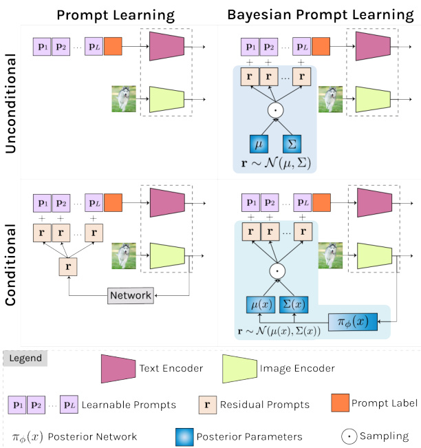
Figure 1: We present a Bayesian perspective on prompt learning by formulating it as a variation al inference problem (right column). Our framework models the prompt space as an a priori distribution which makes our proposal compatible with common prompt learning approaches that are unconditional (top) or conditional on the image (bottom).
图 1: 我们通过将提示学习 (prompt learning) 表述为变分推断问题 (右栏) 提出贝叶斯视角。该框架将提示空间建模为先验分布,使得我们的方案兼容无条件 (顶部) 或图像条件 (底部) 的常见提示学习方法。
Others before us have considered the generalization problem in prompt learning as well, e.g., [55, 54], be it they all seek to optimize a so-called Empirical Risk Minimization. It is, however, well known that Empirical Risk Minimization based models degrade drastically when training and testing distributions are different [37, 2]. To relax the i.i.d. assumption, Peters et al. [37] suggest exploiting the “invariance principle” for better generalization. Unfortunately, Invariant Risk Minimization methods for deep neural networks as of yet fail to deliver competitive results, as observed in [15, 31, 30]. To alleviate this limitation, Lin et al. [30] propose a Bayesian treatment of Invariant Risk Minimization that alleviates over fitting with deep models by defining a regular iz ation term over the posterior distribution of class if i ers, minimizing this term, and pushing the model’s backbone to learn invariant features. We take inspiration from this Bayesian Invariant Risk Minimization [30] and propose the first Bayesian prompt learning approach.
在我们之前,也有研究者考虑过提示学习中的泛化问题,例如[55, 54],但它们都试图优化所谓的经验风险最小化 (Empirical Risk Minimization)。然而众所周知,当训练和测试分布不同时,基于经验风险最小化的模型性能会急剧下降[37, 2]。为放宽独立同分布假设,Peters等人[37]提出利用"不变性原理"来提升泛化能力。但如[15, 31, 30]所述,目前针对深度神经网络的不变风险最小化方法尚未取得理想效果。为缓解这一局限,Lin等人[30]提出了不变风险最小化的贝叶斯处理方法,通过对分类器后验分布定义正则化项、最小化该正则项并推动模型主干学习不变特征,从而缓解深度模型的过拟合问题。我们受此贝叶斯不变风险最小化[30]的启发,提出了首个贝叶斯提示学习方法。
We make three contributions. First, we frame prompt learning from the Bayesian perspective and formulate it as a variation al inference problem (see Figure 1). This formulation provides several benefits. First, it naturally injects noise during prompt learning and induces a regular iz ation term that encourages the model to learn informative prompts, scattered in the prompt space, for each downstream task. As a direct result, we regularize the prompt space, reduce over fitting to seen prompts, and improve generalization on unseen prompts. Second, our framework models the input prompt space in a probabilistic manner, as an a priori distribution which makes our proposal compatible with prompt learning approaches that are unconditional [55] or conditional on the image [54]. Third, we empirically demonstrate on 15 benchmarks that Bayesian prompt learning provides an appropriate coverage of the prompt space, prevents learning spurious features, and exploits transferable invariant features, leading to a better generalization of unseen prompts, even across different datasets and domains.
我们做出三点贡献。首先,我们从贝叶斯视角构建提示学习框架,并将其表述为一个变分推断问题 (参见图1)。这种表述具有多重优势:其一,它自然地在提示学习过程中引入噪声,并产生一个正则化项,促使模型为每个下游任务学习信息丰富且分散在提示空间中的提示。直接效果是规范了提示空间,减少对已见提示的过拟合,提升对未见提示的泛化能力。其二,我们的框架以概率方式对输入提示空间建模,将其作为先验分布,这使得我们的方案兼容无条件[55]或图像条件[54]的提示学习方法。其三,我们在15个基准测试中实证表明,贝叶斯提示学习能恰当覆盖提示空间,避免学习虚假特征,并利用可迁移的不变特征,从而实现对未见提示的更好泛化,甚至跨越不同数据集和领域。
2. Related Work
2. 相关工作
Prompt learning in language. Prompt learning was originally proposed within natural language processing (NLP), by models such as GPT-3 [4]. Early methods constructed prompts by combining words in the language space such that the model would perform better on downstream evaluation [46, 24]. Li and Liang [29] prepend a set of learnable prompts to the different layers of a frozen model and optimize through back-propagation. In parallel, Lester et al. [28] demonstrate that with no intermediate layer pre- fixes or task-specific output layers, adding prefixes alone to the input of the frozen model is enough to compete with fine-tuning. Alternatively, [16] uses a Hyper Network to conditionally generate task-specific and layer-specific prompts pre-pended to the values and keys inside the selfattention layers of a frozen model. Inspired by progress from NLP, we propose a prompt learning method intended for image and language models.
语言中的提示学习。提示学习最初由GPT-3 [4]等模型在自然语言处理(NLP)领域提出。早期方法通过组合语言空间中的词汇构建提示,以提升模型在下游任务中的表现 [46, 24]。Li和Liang [29] 在冻结模型的不同层前添加可学习的提示序列,并通过反向传播进行优化。同时,Lester等人 [28] 证明无需中间层前缀或任务特定输出层,仅需在冻结模型输入前添加前缀即可与微调方法竞争。此外,[16] 采用超网络(Hyper Network)动态生成任务特定和层特定的提示,这些提示被添加到冻结模型自注意力层的键值对中。受NLP领域进展启发,我们提出了一种面向图像与语言模型的提示学习方法。
Prompt learning in image and language. Zhou et al. [55] propose Context Optimization (CoOp), a prompt learner for CLIP, which optimizes prompts in the continuous space through back-propagation. The work demonstrates the benefit of prompt learning over prompt engineering. While CoOp obtains good accuracy on prompts seen during training, it has difficulty generalizing to unseen prompts. It motivated Zhou et al. to introduce Conditional Context Optimization (CoCoOp) [54]. It generates instance-specific prompt residuals through a conditioning mechanism dependent on the image data, which generalizes better.ProGrad by Zhu et al. [56] also strives to bridge the generalization gap by matching the gradient of the prompt to the general knowledge of the CLIP model to prevent forgetting. Alternative directions consist of test-time prompt learning [47], where consistency across multiple views is the supervisory signal, and unsupervised prompt learning [21], where a pseudo-labeling strategy drives the prompt learning. More similar to ours is ProDA by Lu et al. [32], who propose an ensemble of a fixed number of hand-crafted prompts and model the distribution exclusively within the language embedding. Conversely, we prefer to model the input prompt space rather than relying on a fixed number of templates, as it provides us with a mechanism to cover the prompt space by sampling. Moreover, our approach is not limited to unconditional prompt learning from the language embedding, but like Zhou et al. [54], also allows for prompt learning conditioned on an image.
图像与语言中的提示学习。Zhou等人[55]提出了上下文优化(CoOp),一种针对CLIP的提示学习器,通过反向传播在连续空间中优化提示。该工作证明了提示学习相比提示工程的优势。虽然CoOp在训练期间见过的提示上获得了良好的准确性,但难以泛化到未见过的提示。这促使Zhou等人引入了条件上下文优化(CoCoOp)[54],它通过依赖于图像数据的条件机制生成实例特定的提示残差,具有更好的泛化能力。Zhu等人[56]提出的ProGrad也致力于通过将提示的梯度与CLIP模型的通用知识相匹配来弥合泛化差距,以防止遗忘。其他方向包括测试时提示学习47和无监督提示学习21。与我们的方法更相似的是Lu等人[32]提出的ProDA,他们对固定数量的手工提示进行集成,并仅在语言嵌入中建模分布。相反,我们更倾向于对输入提示空间进行建模而非依赖固定数量的模板,这为我们提供了通过采样覆盖提示空间的机制。此外,我们的方法不仅限于从语言嵌入进行无条件提示学习,还能像Zhou等人[54]那样支持以图像为条件的提示学习。
Prompt learning in vision and language. While beyond our current scope, it is worth noting that prompt learning has been applied to a wider range of vision problems and scenarios, which highlights its power and flexibility. Among them are important topics such as unsupervised domain adaptation [13], multi-label classification [49], video classification [25], object detection [9, 12] and pixel-level labelling [40]. Finally, prompt learning has also been applied to vision only models [23, 44] providing an efficient and flexible means to adapt pre-trained models.
视觉与语言中的提示学习。虽然超出了当前讨论范围,但值得注意的是,提示学习已被应用于更广泛的视觉问题和场景,这凸显了其强大性和灵活性。其中包括无监督域适应 [13]、多标签分类 [49]、视频分类 [25]、目标检测 [9,12] 和像素级标注 [40] 等重要课题。最后,提示学习也被应用于纯视觉模型 [23,44],为适应预训练模型提供了高效灵活的手段。
Variation al inference in computer vision. Variation al inference and, more specifically, variation al auto encoder variants have been extensively applied to computer vision tasks as diverse as image generation [39, 43, 42], action recognition [34], instance segmentation [20], few-shot learning [53, 45], domain generalization [10], and continual learning [7]. For example, Zhang et al. [53] focus on the reduction of noise vulnerability and estimation bias in few-shot learning through variation al inference. In the same vein, Du et al. [10] propose a variation al information bottleneck to better manage prediction uncertainty and unknown domains. Our proposed method also shares the advantages of variation al inference in avoiding over fitting in low-shot settings, improving generalization, and encourages the prompt space to be resilient against these challenges. To the best of our knowledge we are the first to introduce variation al inference in prompt learning.
计算机视觉中的变分推断。变分推断,尤其是变分自编码器 (variational autoencoder) 变体,已被广泛应用于各类计算机视觉任务,如图像生成 [39, 43, 42]、动作识别 [34]、实例分割 [20]、少样本学习 [53, 45]、领域泛化 [10] 以及持续学习 [7]。例如,Zhang 等人 [53] 通过变分推断减少少样本学习中的噪声敏感性和估计偏差。类似地,Du 等人 [10] 提出变分信息瓶颈以更好地处理预测不确定性和未知领域。我们提出的方法同样具备变分推断的优势,可避免低样本场景下的过拟合、提升泛化能力,并使提示空间能够抵御这些挑战。据我们所知,这是首次在提示学习中引入变分推断。
3. Method
3. 方法
3.1. Background
3.1. 背景
Contrastive Language-Image Pre training (CLIP) [38] consists of an image encoder $f(\mathbf{x})$ and text encoder $g(\mathbf{t})$ , each producing a $d$ -dimensional $X_{2}$ normalized) embedding from an arbitrary image $\mathbf{x}\in\mathbb{R}^{3\times H\times W}$ , and word embeddings $\textbf{t}\in\mathbb{R}^{L\times e}$ , with $L$ representing the text length and $e$ the embedding dimension1. Both encoders are trained together using a contrastive loss from a large-scale dataset composed of paired images and captions. Once trained, CLIP enables zero-shot $C$ -class image classification by generating each of the $c$ classifier weights $\mathbf{w}{c}$ as the $d$ -dimensional text encoding $g(\mathbf{t}{c})$ . Here $\mathbf{t}{c}$ results from adding the class-specific word embedding $\mathbf{e}{c}$ to a pre-defined prompt $\mathbf{p_{\lambda}}\in\bar{\mathbb{R}}^{L-1\times e}$ , i.e., $\mathbf{w}{c}{=}g(\mathbf{t}{c})$ with $\mathbf{t}{c}={\mathbf{p},\mathbf{e}{c}}$ . The prompt $\mathbf{p}$ is manually crafted to capture the semantic meaning of the downstream task, e.g., $\mathbf{t}_{c}\mathbf{=}^{\mathrm{\tiny~{\left[\Lambda\right]}~}}$ image of a ${\mathtt{c l a s s}}^{\gamma}$ . The probability of image $\mathbf{x}$ being classified as $y\in{1...C}$ is thus defined as $\begin{array}{r}{p(y|\mathbf{x})=\frac{e^{f(\mathbf{x})^{T}\mathbf{w}_{y}}}{\sum_{c}^{C}e^{f(\mathbf{x})^{T}\mathbf{w}_{c}}},}\end{array}$
对比语言-图像预训练 (CLIP) [38] 包含一个图像编码器 $f(\mathbf{x})$ 和文本编码器 $g(\mathbf{t})$ ,分别从任意图像 $\mathbf{x}\in\mathbb{R}^{3\times H\times W}$ 和词嵌入 $\textbf{t}\in\mathbb{R}^{L\times e}$ 生成 $d$ 维 $X_{2}$ 归一化嵌入,其中 $L$ 表示文本长度,$e$ 表示嵌入维度。两个编码器通过对比损失在大规模图文配对数据集上联合训练。训练完成后,CLIP 可通过将每个 $c$ 类分类器权重 $\mathbf{w}{c}$ 生成为 $d$ 维文本编码 $g(\mathbf{t}{c})$ 来实现零样本 $C$ 类图像分类。此处 $\mathbf{t}{c}$ 是将类别特定词嵌入 $\mathbf{e}{c}$ 添加到预定义提示 $\mathbf{p_{\lambda}}\in\bar{\mathbb{R}}^{L-1\times e}$ 的结果,即 $\mathbf{w}{c}{=}g(\mathbf{t}{c})$ 且 $\mathbf{t}{c}={\mathbf{p},\mathbf{e}{c}}$ 。提示 $\mathbf{p}$ 经人工设计以捕获下游任务的语义,例如 $\mathbf{t}_{c}\mathbf{=}^{\mathrm{\tiny~{\left[\Lambda\right]}~}}$ image of a ${\mathtt{c l a s s}}^{\gamma}$ 。图像 $\mathbf{x}$ 被分类为 $y\in{1...C}$ 的概率定义为 $\begin{array}{r}{p(y|\mathbf{x})=\frac{e^{f(\mathbf{x})^{T}\mathbf{w}_{y}}}{\sum_{c}^{C}e^{f(\mathbf{x})^{T}\mathbf{w}_{c}}。}\end{array}$
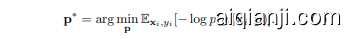
Context Optimization $\mathbf{\mu}(\mathbf{CoOp})$ [55] provides a learned alternative to manually defining prompts. CoOp learns a fixed prompt from a few annotated samples. The prompt is designed as a learnable embedding matrix $\textbf{p}\in\mathbb{R}^{L\times e}$ which is updated via back-propagating the classification error through the frozen CLIP model. Specifically, for a set of $N$ annotated meta-training samples ${{\bf x}{i},y{i}}_{i=1}^{N}$ , the prompt $\mathbf{p}$ is obtained by minimizing the cross-entropy loss, as:
上下文优化 (Context Optimization) $\mathbf{\mu}(\mathbf{CoOp})$ [55] 提供了一种学习替代方案来取代手动定义提示词。CoOp 通过少量标注样本学习固定提示模板,该提示被设计为可学习的嵌入矩阵 $\textbf{p}\in\mathbb{R}^{L\times e}$,通过将分类误差反向传播至冻结的 CLIP 模型中进行更新。具体而言,对于包含 $N$ 个标注元训练样本的集合 ${{\bf x}{i},y{i}}_{i=1}^{N}$,提示 $\mathbf{p}$ 通过最小化交叉熵损失获得,公式为:
Note that this approach, while resembling that of common meta-learning approaches, can still be deployed in a zeroshot scenario provided that for new classes the classification weights will be given by the text encoder. Although this approach generalizes to new tasks with few training iterations, learning a fixed prompt is sensitive to domain shifts between the annotated samples and the unseen prompts.
需要注意的是,这种方法虽然类似于常见的元学习方法,但仍可部署在零样本场景中,前提是新类别的分类权重由文本编码器提供。尽管该方法通过少量训练迭代就能泛化到新任务,但学习固定提示词对标注样本与未见提示之间的领域偏移较为敏感。
Conditional Prompt Learning (CoCoOp) [54] attempts to overcome domain shifts by learning an instancespecific continuous prompt that is conditioned on the input image. To ease the training of a conditional prompt generator, CoCoOp defines each conditional token in a residual way, with a task-specific, learnable set of tokens p and a residual prompt that is conditioned on the input image. Assuming $\mathbf{p}$ to be composed of $L$ learnable tokens $\mathbf{p}{=}[\mathbf{p}{1},\mathbf{p}{2},\cdot\cdot\cdot\mathbf{\delta},\mathbf{p}_{L}]$ , the residual prompt $\mathbf{r}(\mathbf{x}){=}\pi_{\phi}(f(\mathbf{x}))\in\mathbb{R}^{e}$ is produced by a small neural network $\pi_{\phi}$ with as input the image features $f(\mathbf{x})$ . The new prompt is then computed as ${\bf p}({\bf x}){=}[{\bf p}_{1}+{\bf r}({\bf x}),{\bf p}_{2}+$ $\mathbf{r}(\mathbf{x}),\cdots,\mathbf{p}_{L}+\mathbf{r}(\mathbf{x})]$ . The training now comprises learning the task-specific prompt $\mathbf{p}$ and the parameters $\phi$ of the neural network $\pi_{\phi}$ . Defining the context-specific text embedding ${\bf t}_{c}({\bf x}){=}{{\bf p}({\bf x}),{\bf e}_{c}}$ , and $p(y\vert\mathbf{x})$ as :
条件提示学习 (CoCoOp) [54] 试图通过学习一个基于输入图像的条件化实例特定连续提示来克服领域偏移。为了简化条件提示生成器的训练,CoCoOp以残差方式定义每个条件token,包含一组任务特定的可学习token p和一个基于输入图像的残差提示。假设$\mathbf{p}$由$L$个可学习token组成$\mathbf{p}{=}[\mathbf{p}{1},\mathbf{p}{2},\cdot\cdot\cdot\mathbf{\delta},\mathbf{p}_{L}]$,残差提示$\mathbf{r}(\mathbf{x}){=}\pi_{\phi}(f(\mathbf{x}))\in\mathbb{R}^{e}$由一个小型神经网络$\pi_{\phi}$生成,其输入为图像特征$f(\mathbf{x})$。新提示通过${\bf p}({\bf x}){=}[{\bf p}_{1}+{\bf r}({\bf x}),{\bf p}_{2}+$$\mathbf{r}(\mathbf{x}),\cdots,\mathbf{p}_{L}+\mathbf{r}(\mathbf{x})]$计算得出。训练过程包括学习任务特定提示$\mathbf{p}$和神经网络$\pi_{\phi}$的参数$\phi$。定义上下文特定文本嵌入${\bf t}_{c}({\bf x}){=}{{\bf p}({\bf x}),{\bf e}_{c}}$,并将$p(y\vert\mathbf{x})$表示为:

the learning is formulated as:
学习被表述为:

While CoCoOp achieves good results in many downstream tasks, it is still prone to the domain shift problem, considering that $\pi_{\phi}$ provides a deterministic residual prompt from the domain-specific image features $f(\mathbf{x})$ .
尽管CoCoOp在许多下游任务中取得了良好效果,但由于$\pi_{\phi}$从领域特定图像特征$f(\mathbf{x})$中生成的是确定性残差提示,它仍然容易受到领域偏移问题的影响。
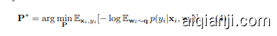
Prompt Distribution Learning (ProDA) [32] learns a distribution of prompts that generalize to a broader set of tasks. It learns a collection of prompts P={pk}kK=1 that subsequently generate an a posteriori distribution of the classifier weights for each of the target classes. For a given mini-batch of $K$ sampled prompts $\mathbf{p}{k}\mathrm{\sim}\mathbf{P}$ , the classifier weights $\mathbf{w}{c}$ are sampled from the posterior distribution $\mathbf{q}{=}\mathcal{N}(\mu_{\mathbf{w}_{1:C}},\Sigma_{\mathbf{w}_{1:C}})$ , with mean $\mu_{\mathbf{w}_{1:C}}$ and covariance $\Sigma_{{\bf w}_{1:C}}$ computed from the collection ${\mathbf{w}_{k,c}{=}g(\mathbf{t}_{k,c})}_{c=1:C,k=1:K}$ , with $\mathbf{t}_{k,c}~=~\left{\mathbf{p}_{k},\mathbf{e}_{c}\right}$ . The objective is formulated as:
提示分布学习 (Prompt Distribution Learning, ProDA) [32] 通过学习一组泛化性更强的提示分布来适应更广泛的任务。该方法学习一组提示集合 P={pk}kK=1,随后为每个目标类别生成分类器权重的后验分布。对于给定的包含 $K$ 个采样提示 $\mathbf{p}{k}\mathrm{\sim}\mathbf{P}$ 的小批量数据,分类器权重 $\mathbf{w}{c}$ 从后验分布 $\mathbf{q}{=}\mathcal{N}(\mu_{\mathbf{w}_{1:C}},\Sigma_{\mathbf{w}_{1:C}})$ 中采样得到,其均值 $\mu_{\mathbf{w}_{1:C}}$ 和协方差 $\Sigma_{{\bf w}_{1:C}}$ 由集合 ${\mathbf{w}_{k,c}{=}g(\mathbf{t}_{k,c})}_{c=1:C,k=1:K}$ 计算得出,其中 $\mathbf{t}_{k,c}~=~\left{\mathbf{p}_{k},\mathbf{e}_{c}\right}$。目标函数定义为:
Computing $\mathbb{E}{\mathbf{w}{l}}p(y_{i}|\mathbf{x}{i},\mathbf{w}{l})]$ is intractable and an upper bound to Eq. 4 is derived. During inference, the classifier weights are set to those given by the predictive mean $\mathbf{w}{c}{=}\mu{\mathbf{w}_{1:C}}$ , computed across the set of learned prompts $\mathbf{P}$ .
计算 $\mathbb{E}{\mathbf{w}{l}}p(y_{i}|\mathbf{x}{i},\mathbf{w}{l})]$ 是不可行的,因此推导出式4的上界。在推理过程中,分类器权重设置为预测均值 $\mathbf{w}{c}{=}\mu{\mathbf{w}_{1:C}}$ ,该均值通过已学习的提示集 $\mathbf{P}$ 计算得出。
3.2. Conditional Bayesian Prompt Learning
3.2. 条件贝叶斯提示学习
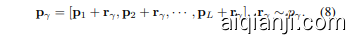
We propose to model the input prompt space in a probabilistic manner, as an a priori, conditional distribution. We define a distribution $p_{\gamma}$ over the prompts $\mathbf{p}$ that is conditional on the image, i.e., ${\bf p}\sim p_{\gamma}({\bf x})$ . To this end, we as- sume that $\mathbf{p}$ can be split into a fixed set of prompts $\mathbf{p}_{i}$ and an conditional residual prompt $\mathbf{r}$ that act as a latent variable over p. The conditional prompt is then defined as:
我们提出以概率方式对输入提示空间进行建模,将其视为一个先验条件分布。我们定义了一个基于图像条件的提示分布 $p_{\gamma}$ ,即 ${\bf p}\sim p_{\gamma}({\bf x})$ 。为此,我们假设 $\mathbf{p}$ 可拆分为固定提示集 $\mathbf{p}_{i}$ 和作为潜在变量的条件残差提示 $\mathbf{r}$ ,此时条件提示定义为:

where $p_{\gamma}(\mathbf{x})$ refers to the real posterior distribution over $\mathbf{r}$ conditioned on the observed features $\mathbf{x}$ . Denoting the class
其中 $p_{\gamma}(\mathbf{x})$ 表示基于观测特征 $\mathbf{x}$ 条件下 $\mathbf{r}$ 的真实后验分布。设类别
specific input as $\mathbf{t}{c,\gamma}(\mathbf{x}){=}{\mathbf{p}{\gamma}(\mathbf{x}),\mathbf{e}_{c}}$ , the marginal likelihood $p(y\vert\mathbf{x})$ is:
特定输入为 $\mathbf{t}{c,\gamma}(\mathbf{x}){=}{\mathbf{p}{\gamma}(\mathbf{x}),\mathbf{e}_{c}}$ 时,边缘似然 $p(y\vert\mathbf{x})$ 为:

Solving Eq. 3 with the marginal likelihood from Eq. 6 is intractable, as it requires computing $p_{\gamma}(\mathbf{r}|\mathbf{x})p_{\gamma}(\mathbf{x})$ . Instead, we resort to deriving a lower bound by introducing a variational posterior distribution $\pi_{\phi}(\mathbf{x})$ from which the residual $\mathbf{r}_{\gamma}$ can be sampled. The variation al bound is defined as:
利用式6中的边缘似然来求解式3是不可行的,因为它需要计算 $p_{\gamma}(\mathbf{r}|\mathbf{x})p_{\gamma}(\mathbf{x})$ 。为此,我们转而通过引入变分后验分布 $\pi_{\phi}(\mathbf{x})$ 来推导下界,残差 $\mathbf{r}_{\gamma}$ 可从该分布中采样。变分下界定义为:

with $p(y|\mathbf{x},\mathbf{r}){\propto}e^{f(\mathbf{x})^{T}g(\mathbf{t}{c,\gamma}(\mathbf{x}))}$ , where the dependency on $\mathbf{r}$ comes through the definition of $\mathbf{t}{c,\gamma}$ . Following standard variation al optimization practices [26, 14], we define $\pi_{\phi}$ as a Gaussian distribution conditioned on the input image features $\mathbf{x}$ , as $\mathbf{r}(\mathbf{x}){\sim}\mathcal{N}(\mu(\mathbf{x}),\Sigma(\mathbf{x}))$ , with $\mu$ and $\Sigma$ parameterized by two linear layers followed by two linear heads on top to estimate the $\mu$ and $\Sigma$ of the residual distribution. The prior $p_{\gamma}(\mathbf{r})$ is defined as $\mathcal{N}(\mathbf{0},\mathbf{I})$ , and we use the reparameterization trick to generate Monte-Carlo samples from $\pi_{\phi}$ to maximize the right side of Eq. 7. The optimization of Eq. 7 comprises learning the prompt embeddings ${\mathbf{p}{i}}{i=1}^{L}$ as well as the parameters of the posterior network $\pi_{\phi}$ and the linear layers parameter i zing $\mu$ and $\Sigma$ . Note that this adds little complexity as it requires learning $\mathbf{p}$ and $\pi_{\phi}$ , given that $\mu$ and $\Sigma$ are defined as two linear layers on top of $\pi_{\phi}$ .
其中 $p(y|\mathbf{x},\mathbf{r}){\propto}e^{f(\mathbf{x})^{T}g(\mathbf{t}{c,\gamma}(\mathbf{x}))}$ ,$\mathbf{r}$ 的依赖性通过 $\mathbf{t}{c,\gamma}$ 的定义体现。遵循标准变分优化实践 [26, 14],我们将 $\pi_{\phi}$ 定义为以输入图像特征 $\mathbf{x}$ 为条件的高斯分布,即 $\mathbf{r}(\mathbf{x}){\sim}\mathcal{N}(\mu(\mathbf{x}),\Sigma(\mathbf{x}))$ ,其中 $\mu$ 和 $\Sigma$ 由两个线性层参数化,并通过顶部的两个线性头分别估计残差分布的 $\mu$ 和 $\Sigma$。先验 $p_{\gamma}(\mathbf{r})$ 定义为 $\mathcal{N}(\mathbf{0},\mathbf{I})$ ,并采用重参数化技巧从 $\pi_{\phi}$ 生成蒙特卡洛样本以最大化式7右侧。式7的优化包括学习提示嵌入 ${\mathbf{p}{i}}{i=1}^{L}$ 以及后验网络 $\pi_{\phi}$ 的参数,还有参数化 $\mu$ 和 $\Sigma$ 的线性层。需注意,由于 $\mu$ 和 $\Sigma$ 被定义为 $\pi_{\phi}$ 顶部的两个线性层,该方法仅需学习 $\mathbf{p}$ 和 $\pi_{\phi}$ ,复杂度增加有限。
Inference. At test time, $K$ residuals are sampled from the conditional distribution $\pi_{\phi}(\mathbf{x})$ , which are used to generate $K$ different prompts per class $\mathbf{p}{k}{=}[\mathbf{p}{1}\mathbf{\beta}+$ $\mathbf{r}{k},\mathbf{p}{2}+\mathbf{r}{k},\cdots,\mathbf{p}{L}+\mathbf{r}{k}]$ . Each prompt is prepended to the class-specific embedding to generate a series of $K$ separate classifier weights $\mathbf{w}{k,c}$ . We then compute $\begin{array}{r}{p(y=c|\mathbf x){=}(1/K)\sum_{k=1}^{K}p(y{=}c|\mathbf x,\mathbf w_{k,c})}\end{array}$ and select $\hat{c}{=}\arg\operatorname*{max}_{c}p(y{=}c|\mathbf{x})$ as the predicted class. It is worth noting that because the posterior distribution is generated by the text encoder, it is not expected that for $K\rightarrow\infty$ , $\begin{array}{r}{(1/K)\sum_{k}p(y=c\mid\mathbf{x},\mathbf{w}_{c,k})~\to~p(y=c|\mathbf{x},g({\mu(\mathbf{x}),\mathbf{e}_{c}})}\end{array}$ , meanin g that sampling at inference time remains relevant.
推理。在测试时,从条件分布 $\pi_{\phi}(\mathbf{x})$ 中采样 $K$ 个残差,用于为每个类别生成 $K$ 个不同的提示 $\mathbf{p}{k}{=}[\mathbf{p}{1}\mathbf{\beta}+$ $\mathbf{r}{k},\mathbf{p}{2}+\mathbf{r}{k},\cdots,\mathbf{p}{L}+\mathbf{r}{k}]$。每个提示被添加到类别特定的嵌入前,生成一系列 $K$ 个独立的分类器权重 $\mathbf{w}{k,c}$。然后计算 $\begin{array}{r}{p(y=c|\mathbf x){=}(1/K)\sum_{k=1}^{K}p(y{=}c|\mathbf x,\mathbf w_{k,c})}\end{array}$ 并选择 $\hat{c}{=}\arg\operatorname*{max}_{c}p(y{=}c|\mathbf{x})$ 作为预测类别。值得注意的是,由于后验分布由文本编码器生成,当 $K\rightarrow\infty$ 时,$\begin{array}{r}{(1/K)\sum_{k}p(y=c\mid\mathbf{x},\mathbf{w}_{c,k})~\to~p(y=c|\mathbf{x},g({\mu(\mathbf{x}),\mathbf{e}_{c}})}\end{array}$ 并不成立,这意味着推理时的采样仍然具有实际意义。
3.3. Unconditional Bayesian Prompt Learning
3.3. 无条件贝叶斯提示学习 (Unconditional Bayesian Prompt Learning)
Notably, our framework can also be reformulated as an unconditional case by simply removing the dependency of the input image from the latent distribution. In such a scenario, we keep a fixed set of prompt embeddings and learn a global latent distribution $p_{\gamma}$ over the residual prompts $\mathbf{r}$ , as $\mathbf{r}\sim\mathcal{N}(\boldsymbol{\mu},\boldsymbol{\Sigma})$ , where $\mu$ and $\Sigma$ are parameterized by two learnable vectors. To this end, we assume that $\mathbf{p}$ can be split into a fixed set of prompts $\mathbf{p}_{i}$ and a residual prompts $\mathbf{r}$ that act as a latent variable over $\mathbf{p}$ . For the unconditional case, the prompt is defined as:
值得注意的是,我们的框架也可以通过简单地从潜在分布中移除输入图像的依赖性,重新表述为无条件情况。在这种场景下,我们保留一组固定的提示嵌入 (prompt embeddings) ,并在残差提示 (residual prompts) $\mathbf{r}$ 上学习一个全局潜在分布 $p_{\gamma}$ ,即 $\mathbf{r}\sim\mathcal{N}(\boldsymbol{\mu},\boldsymbol{\Sigma})$ ,其中 $\mu$ 和 $\Sigma$ 由两个可学习向量参数化。为此,我们假设 $\mathbf{p}$ 可以拆分为一组固定的提示 $\mathbf{p}_{i}$ 和一个作为 $\mathbf{p}$ 潜在变量的残差提示 $\mathbf{r}$ 。对于无条件情况,提示定义为:
In this case, $p_{\gamma}$ is a general distribution learned during training with no dependency on the input sample x.
在这种情况下,$p_{\gamma}$ 是训练期间学习到的通用分布,不依赖于输入样本 x。
Having defined both unconditional Bayesian prompt learning and conditional Bayesian prompt learning we are now ready to evaluate their generalization ability.
在定义了无条件贝叶斯提示学习 (unconditional Bayesian prompt learning) 和有条件贝叶斯提示学习 (conditional Bayesian prompt learning) 后,我们现在可以评估它们的泛化能力了。
4. Experiments and Results 4.1. Experimental Setup
4. 实验与结果 4.1. 实验设置
Three tasks and fifteen datasets. We consider three tasks: unseen prompts generalization, cross-dataset prompts generalization, and cross-domain prompts generalization. For the first two tasks, we rely on the same 11 image recognition datasets as Zhou et al. [55, 54]. These include image classification (ImageNet [6] and Caltech101 [11]), fine-grained classification (OxfordPets [36], Stanford Cars [27], Flowers102 [35], Food101 [3] and FG VC Aircraft [33]), scene recognition (SUN397 [52]), action recognition (UCF101 [48]), texture classification (DTD [5]), and satellite imagery recognition (Eu- roSAT [17]). For cross-domain prompts generalization, we train on ImageNet and report on ImageNetV2 [41], ImageNet-Sketch [51], ImageNet-A [19], and ImageNetR [18].
三项任务和十五个数据集。我们考虑三项任务:未见提示泛化、跨数据集提示泛化和跨领域提示泛化。对于前两项任务,我们采用与Zhou等人[55, 54]相同的11个图像识别数据集,包括图像分类(ImageNet [6]和Caltech101 [11])、细粒度分类(OxfordPets [36]、Stanford Cars [27]、Flowers102 [35]、Food101 [3]和FG VC Aircraft [33])、场景识别(SUN397 [52])、动作识别(UCF101 [48])、纹理分类(DTD [5])以及卫星图像识别(EuroSAT [17])。对于跨领域提示泛化任务,我们在ImageNet上训练,并在ImageNetV2 [41]、ImageNet-Sketch [51]、ImageNet-A [19]和ImageNetR [18]上进行测试。
Evaluation metrics. For all three tasks we report average accuracy and standard deviation.
评估指标。针对所有三项任务,我们均报告平均准确率及标准差。
Implementation details. Our conditional variation al prompt learning contains three sub-networks: an image encoder $f(\mathbf{x})$ , a text encoder $g(\mathbf{t})$ , and a posterior network $\pi_{\phi}$ . The image encoder $f(\mathbf{x})$ is a ViT-B/16 [8] and the text encoder $g(\mathbf{t})$ a transformer [50], which are both initialized with CLIP’s pre-trained weights and kept frozen during training, as in [55, 54]. The posterior network $\pi_{\phi}$ consists of two linear layers followed by an ELU activation function as trunk and two linear heads on top to estimate the $\mu$ and $\Sigma$ of the residual distribution. For each task and dataset, we optimize the number of samples $K$ and epochs. Other hyper-parameters as well as the training pipeline in terms of few-shot task definitions are identical to [55, 54] (see Table 9 and 10 in the appendix).
实现细节。我们的条件变分提示学习包含三个子网络:图像编码器 $f(\mathbf{x})$、文本编码器 $g(\mathbf{t})$ 和后验网络 $\pi_{\phi}$。图像编码器 $f(\mathbf{x})$ 采用 ViT-B/16 [8] 架构,文本编码器 $g(\mathbf{t})$ 基于 Transformer [50] 架构,二者均使用 CLIP 预训练权重初始化并在训练期间保持冻结,如 [55, 54] 所述。后验网络 $\pi_{\phi}$ 由两个线性层和 ELU 激活函数构成主干,顶部通过两个线性头部分别估计残差分布的 $\mu$ 和 $\Sigma$。针对每个任务和数据集,我们优化样本数 $K$ 和训练周期数。其他超参数及少样本任务定义相关的训练流程均与 [55, 54] 保持一致(详见附录表 9 和表 10)。
4.2. Comparisons
4.2. 对比
We first compare against CoOp [55], CoCoOp [54], and ProDA [32] in terms of the generalization of learned prompts on unseen classes, datasets, or domains. For $\mathrm{CoOp}$ and $\mathrm{{CoCoOp}}$ , all results are adopted from [54], and we report results for ProDA using our re-implementation.
我们首先在未见过的类别、数据集或领域的提示泛化能力方面,与CoOp [55]、CoCoOp [54]和ProDA [32]进行对比。对于$\mathrm{CoOp}$和$\mathrm{CoCoOp}$,所有结果均引自[54],而ProDA的结果则基于我们的复现实现。
Task I: unseen prompts generalization We report the unseen prompts generalization of our method on 11 datasets for three different random seeds. Each dataset is divided into two disjoint subsets: seen classes and unseen classes. We train our method on the seen classes and evaluate it on the unseen classes. For a fair comparison, we follow [55, 54] in terms of dataset split and number of shots. From
任务 I: 未见提示泛化性
我们在11个数据集上针对三种不同随机种子报告了本方法的未见提示泛化性能。每个数据集被划分为两个互斥子集:已见类别和未见类别。我们在已见类别上训练方法,并在未见类别上评估其表现。为公平比较,我们遵循[55, 54]的数据集划分和样本数量设置。
Table 1: Task I: unseen prompts generalization comparison between conditional Bayesian prompt learning and alternatives. Our model provides better generalization on unseen prompts compared to CoOp, $\mathrm{{CoCoOp}}$ and ProDA.
表 1: 任务一:条件贝叶斯提示学习与其他方法在未见提示泛化能力上的对比。相比CoOp、$\mathrm{{CoCoOp}}$和ProDA,我们的模型在未见提示上展现出更好的泛化性能。
| CoOp [55] | CoCo0p [54] | ProDA [32] | Ours | |
|---|---|---|---|---|
| Caltech101 | 89.81 | 93.81 | 93.23 | 94.93±0.1 |
| DTD | 41.18 | 56.00 | 56.48 | 60.80±0.5 |
| EuroSAT | 54.74 | 60.04 | 66.00 | 75.30±0.7 |
| FGVCAircraft | 22.30 | 23.71 | 34.13 | 35.00±0.5 |
| Flowers102 | 59.67 | 71.75 | 68.68 | 70.40±1.8 |
| Food101 | 82.26 | 91.29 | 88.57 | 92.13±0.1 |
| ImageNet | 67.88 | 70.43 | 70.23 | 70.93±0.1 |
| OxfordPets | 95.29 | 97.69 | 97.83 | 98.00±0.1 |
| StanfordCars | 60.40 | 73.59 | 71.20 | 73.23±0.2 |
| SUN397 | 65.89 | 76.86 | 76.93 | 77.87±0.5 |
| UCF101 | 56.05 | 73.45 | 71.97 | 75.77±0.1 |
| Average | 63.22 | 71.69 | 72.30 | 74.94±0.2 |
Table 1, it can be seen that our best-performing method, conditional Bayesian prompt learning, outperforms $\mathrm{{CoOp}}$ and $\mathbf{CoCoOp}$ in terms of unseen prompts generalization by $11.72%$ and $3.25%$ , respectively. Our proposal also demonstrates minimal average variance across all datasets. This is achieved by regularizing the optimization by virtue of the variation al formulation. Moreover, our model also performs better than ProDA [32], its probabilistic counterpart, by $2.64%$ . This mainly happens because our proposed method learns the prompt distribution directly in the prompt space and allows us to sample more informative prompts for the downstream tasks.
表 1: 可以看出,我们表现最佳的条件贝叶斯提示学习 (conditional Bayesian prompt learning) 方法在未见提示泛化能力上分别以 11.72% 和 3.25% 的优势超越了 $\mathrm{CoOp}$ 和 $\mathbf{CoCoOp}$。我们的方案在所有数据集上也展现出最小的平均方差,这是通过变分公式对优化过程进行正则化实现的。此外,我们的模型性能还以 2.64% 的优势优于其概率对应方法 ProDA [32],这主要归因于我们提出的方法直接在提示空间中学习提示分布,从而能为下游任务采样信息量更丰富的提示。
Task II: cross-dataset prompts generalization For the next task, cross-dataset prompts generalization, the model is trained on a source dataset (ImageNet) and then assessed on 10 distinct target datasets. This experiment tries to determine how effectively our method generalizes beyond the scope of a single dataset. As reported in Table 2, our conditional Bayesian prompt learning outperforms $\mathrm{{CoOp}}$ and $\mathrm{CoCoOp}$ on the target dataset by $2.07%$ and $0.36%$ . This highlights that our method encourages the model to exploit transferable invariant features beneficial for datasets with a non-overlapping label space. Furthermore, our method improves accuracy for 7 out of 10 target datasets. Unlike CoCoOp, which performs better in ImageNet-like datasets such as Caltech101 and Stanford Cars, our Bayesian method exhibits improvement on dissimilar datasets (e.g., FGVCAircraft, DTD, and EuroSAT), demonstrating its capacity to capture the unique characteristics of each dataset.
任务二:跨数据集提示泛化
在跨数据集提示泛化任务中,模型先在源数据集(ImageNet)上训练,随后在10个不同的目标数据集上评估。该实验旨在验证我们的方法在单一数据集范围之外的泛化能力。如表2所示,我们的条件贝叶斯提示学习在目标数据集上分别以2.07%和0.36%的优势超过$\mathrm{CoOp}$与$\mathrm{CoCoOp}$。这表明我们的方法能促使模型利用可迁移的不变特征,这对具有非重叠标签空间的数据集尤为有益。此外,我们的方法在10个目标数据集中的7个上实现了精度提升。与CoCoOp在类ImageNet数据集(如Caltech101和Stanford Cars)表现更好不同,我们的贝叶斯方法在差异较大的数据集(如FGVCAircraft、DTD和EuroSAT)上展现出改进,证明其能捕捉不同数据集的独特特征。
Task III: cross-domain prompts generalization Lastly, we examine our conditional Bayesian prompt learning through the lens of distribution shift and robustness. We train our model on the source dataset ImageNet for three different random seeds, and assess it on ImageNetV2, ImageNet-Sketch, ImageNet-A, and ImageNet-R. Prior works such as CoOp [55] and CoCoOp [54] demonstrate empirically that learning a soft-prompt improves the model’s resilience against distribution shift and adversarial attack. Following their experiments, we are also interested in determining if treating prompts in a Bayesian manner maintains or improves performance. As reported in Table 2 compared with $\mathrm{{CoOp}}$ , our method improves the performance on ImageNet-Sketch, ImageNet-A, and ImageNetR by $1.21%$ , $1.62%$ , and $1.79%$ . Compared with $\mathrm{{CoCoOp}}$ , our proposed method consistently enhances the model accuracy on ImageNetV2, ImageNet-Sketch, ImageNet-A, and ImageNet-R by $0.16%$ , $0.45%$ , $0.7%$ , and $0.82%$ . This is because our proposed method prevents learning spurious features, e.g., high-frequency features, and instead learns invariant ones by virtue of the Bayesian formulation.
任务三:跨域提示泛化
最后,我们从分布偏移和鲁棒性的角度检验条件贝叶斯提示学习。我们在源数据集ImageNet上以三种不同的随机种子训练模型,并在ImageNetV2、ImageNet-Sketch、ImageNet-A和ImageNet-R上评估。先前工作如CoOp [55]和CoCoOp [54]通过实验证明,学习软提示能提升模型对分布偏移和对抗攻击的鲁棒性。基于这些实验,我们同样关注以贝叶斯方式处理提示是否能保持或提升性能。如表2所示,与$\mathrm{{CoOp}}$相比,我们的方法在ImageNet-Sketch、ImageNet-A和ImageNet-R上的性能分别提升了$1.21%$、$1.62%$和$1.79%$。与$\mathrm{{CoCoOp}}$相比,所提方法在ImageNetV2、ImageNet-Sketch、ImageNet-A和ImageNet-R上的模型准确率分别持续提高了$0.16%$、$0.45%$、$0.7%$和$0.82%$。这是因为所提方法通过贝叶斯公式避免了学习虚假特征(如高频特征),转而学习不变特征。
Table 2: Task II: cross-dataset prompts generalization. Our proposed model is evaluated on 11 datasets with different label spaces. As shown, conditional Bayesian prompt learning performs better than non-Bayesian alternatives on 7 out of 10 datasets. Task III: cross-domain prompts genera liz ation. Our model is evaluated on four datasets sharing the same label space as the training data. Our method outperforms alternatives on 3 out of 4 datasets.
表 2: 任务II: 跨数据集提示泛化。我们提出的模型在11个具有不同标签空间的数据集上进行评估。结果显示,条件贝叶斯提示学习在10个数据集中的7个上优于非贝叶斯方法。任务III: 跨领域提示泛化。我们的模型在与训练数据共享相同标签空间的四个数据集上进行评估。我们的方法在4个数据集中的3个上优于其他方法。
| CoOp [55] | CoCoOp [54] | Ours |
|---|---|---|
| 任务II: 跨数据集提示泛化 | ||
| Caltech101 93.70 | 94.43 | 93.67±0.2 |
| DTD 41.92 | 45.73 | 46.10±0.1 |
| EuroSAT 46.39 | 45.37 | 45.87±0.7 |
| FGVCAircraft 18.47 | 22.94 | 24.93±0.2 |
| Flowers102 68.71 | 70.20 | 70.90±0.1 |
| Food101 85.30 | 86.06 | 86.30±0.1 |
| OxfordPets 89.14 | 90.14 | 90.63±0.1 |
| StanfordCars 64.51 | 65.50 | 65.00±0.1 |
| SUN397 64.15 | 67.36 | 67.47±0.1 |
| UCF101 66.55 | 68.21 | 68.67±0.2 |
| Average 63.88 | 65.59 | 65.95±0.2 |
| 任务III: 跨领域提示泛化 | ||
| ImageNetV2 | 64.20 64.07 | 64.23±0.1 |
| ImageNet-Sketch | 47.99 48.75 | 49.20±0.0 |
| ImageNet-A 49.71 | 50.63 | 51.33±0.1 |
| ImageNet-R 75.21 | 76.18 | 77.00±0.1 |
| Average | 59.27 59.88 | 60.44±0.1 |
Table 3: In-domain performance. CoOp provides the best in-domain performance, but suffers from distribution shifts. Our proposal provides the best trade-off.
表 3: 领域内性能。CoOp 提供了最佳的领域内性能,但在分布偏移时表现不佳。我们的方案提供了最佳的权衡。
| CoOp [55] | CoCo0p [54] | ProDA [32] | Ours | |
|---|---|---|---|---|
| TaskI | 82.66 | 80.47 | 81.56 | 80.10±0.1 |
| Task II (III) | 71.51 | 71.02 | 70.70±0.2 |
In-domain performance Different from other prompt works, we focus on prompt generalization when we have distribution shift in the input space, the label space, or both.
域内性能
与其他提示工作不同,我们关注的是当输入空间、标签空间或两者同时存在分布偏移时提示的泛化能力。
Table 4: Effect of variation al formulation. Formulating prompt learning as variation al inference improves model generalization on unseen prompts compared to a non-Bayesian baseline [55], for both the unconditional and conditional setting.
表 4: 变分公式的效果。与非贝叶斯基线 [55] 相比,将提示学习 (prompt learning) 表述为变分推断 (variational inference) 能提升模型在未见提示上的泛化能力,该结论在无条件设定和条件设定下均成立。
| DTD | EuroSAT | FGVC | Flowers102 | UCF101 | |
|---|---|---|---|---|---|
| Baseline | 41.18 | 54.74 | 22.30 | 59.67 | 56.05 |
| Unconditional | 58.70 | 71.63 | 33.80 | 75.90 | 74.63 |
| Conditional | 60.80 | 75.30 | 35.00 | 70.40 | 75.77 |
Table 5: Benefit of the posterior distribution. The con- ditional posterior distribution $\mathcal{N}(\mu(\mathbf{x}),\Sigma(\mathbf{x}))$ outperforms the two distributions $\mathcal{U}(0,1)$ and $\mathcal{N}(0,\mathrm{I})$ by a large margin for all datasets, indicating that the conditional variant captures more informative knowledge regarding the underlying distribution of prompts in the prompt space.
表 5: 后验分布的优势。条件后验分布 $\mathcal{N}(\mu(\mathbf{x}),\Sigma(\mathbf{x}))$ 在所有数据集上均大幅优于 $\mathcal{U}(0,1)$ 和 $\mathcal{N}(0,\mathrm{I})$ 两种分布,表明条件变体能捕获提示空间中关于提示底层分布的更多信息知识。
| DTD | EuroSAT | FGVC | Flowers102 | UCF101 | |
|---|---|---|---|---|---|
| u(0,1) | 33.20 | 54.20 | 10.50 | 45.30 | 55.70 |
| N(0, 1) | 26.60 | 50.00 | 07.70 | 36.10 | 48.80 |
| N(μ(x),∑(x)) | 56.40 | 64.50 | 33.00 | 72.30 | 75.60 |
| N(μ(x),0) | 59.80 | 59.90 | 34.10 | 73.50 | 76.50 |
For reference, we provide the in-domain average performance in Table 3. As expected, our generalization ability comes with reduced over fitting on the in-domain setting, leading to $\mathrm{CoOp}$ exhibiting better in-domain performance. However, when comparing average results in Tables 1, 2 and 3, our proposal brings the best trade-off and we maintain performance on the in-domain setting while delivering a consistent performance gain on the out-of-domain setting.
作为参考,我们在表3中提供了域内平均性能。正如预期的那样,我们的泛化能力减少了对域内设置的过拟合,使得 $\mathrm{CoOp}$ 展现出更好的域内性能。然而,通过比较表1、表2和表3的平均结果,我们的方案带来了最佳权衡,在保持域内设置性能的同时,在域外设置上实现了持续的性能提升。
4.3. Ablations
4.3. 消融实验
Effect of variation al formulation. When prompt learning is formulated as a variation al inference problem, it improves model generalization by regularizing the prompt space. To demonstrate this, we first report the model performances on unseen prompts for DTD, EuroSAT, FGVCAircraft, Flowers102, and UCF101 in Table 4. Regardless of whether a variation al formulation is unconditional or conditional, it consistently increases unseen prompt genera liz ation compared with the CoOp baseline [55]. This is achieved by sampling more informative prompts and better coverage of the prompt space (which we detail in a following ablation). Moreover, conditional variation al prompt learning enhances the model performance on 4 out of 5 datasets compared to its unconditional counterpart, indicating its effectiveness in capturing the prompt distribution. This happens as the conditional formulation provides us with the potential to successfully capture fine-grained prompts by conditioning on the input image.
变分公式的影响。当提示学习被构建为变分推断问题时,它通过正则化提示空间来提升模型泛化能力。为验证这一点,我们首先在表4中报告了DTD、EuroSAT、FGVCAircraft、Flowers102和UCF101数据集上未见提示的模型性能。无论变分公式是无条件还是条件形式,相比CoOp基线[55],它都能持续提升未见提示的泛化能力。这是通过采样信息量更大的提示和更好地覆盖提示空间实现的(我们将在后续消融实验中详述)。此外,条件变分提示学习在5个数据集中的4个上表现优于无条件变体,表明其捕捉提示分布的有效性。这是因为条件公式通过以输入图像为条件,为我们提供了成功捕捉细粒度提示的可能性。
Benefit of the posterior distribution $q_{\phi}$ . We ablate the effectiveness of the variation al posterior distribution. To do so, we consider sampling one residual prompt from the uniform distribution $\mathcal{U}(0,1)$ , normal distribution $\mathcal{N}(0,\mathrm{I})$ , normal distribution $\mathcal{N}(\mu(\mathbf{x}),\Sigma(\mathbf{x}))$ , and normal distribution $\mathcal{N}(\mu(\mathbf{x}),0)$ and report the unseen prompts accuracy for one random seed in Table 5. we find that drawing one sample from $\mathcal{N}(\mu(\mathbf{x}),\Sigma(\mathbf{x}))$ yields superior results compared to drawing one sample from uniform distribution $\mathcal{U}(0,1)$ and normal distribution $\mathcal{N}(0,\mathrm{I})$ , demonstrating the informativeness of the prompt samples generated by our conditional setting. In addition, except for the EuroSAT dataset, a sample from the normal distribution $\mathcal{N}(\mu(\mathbf{x}),0)$ obtains the best performance in comparison with alternatives, indicating the mean of the normal distribution $\mu({\bf x})$ is the most effective sample.
后验分布 $q_{\phi}$ 的优势。我们通过消融实验验证变分后验分布的有效性。具体做法是从均匀分布 $\mathcal{U}(0,1)$、正态分布 $\mathcal{N}(0,\mathrm{I})$、正态分布 $\mathcal{N}(\mu(\mathbf{x}),\Sigma(\mathbf{x}))$ 以及正态分布 $\mathcal{N}(\mu(\mathbf{x}),0)$ 中各采样一个残差提示 (residual prompt),并在表5中报告单次随机种子下的未见提示准确率。实验表明,与从均匀分布 $\mathcal{U}(0,1)$ 和正态分布 $\mathcal{N}(0,\mathrm{I})$ 采样相比,从 $\mathcal{N}(\mu(\mathbf{x}),\Sigma(\mathbf{x}))$ 采样能获得更优结果,这证明我们条件设置生成的提示样本具有信息量。此外,除EuroSAT数据集外,从正态分布 $\mathcal{N}(\mu(\mathbf{x}),0)$ 采样的表现优于其他方案,说明正态分布均值 $\mu({\bf x})$ 是最有效的采样点。
Table 6: Influence of Monte Carlo sampling on unseen prompts accuracy. As demonstrated, increasing the number of Monte Carlo samples boosts performance initially but reaches a plateau after 20 samples for all datasets.
表 6: 蒙特卡洛采样对未见提示词准确率的影响。如表所示,增加蒙特卡洛采样数量初期能提升性能,但在所有数据集上达到20个样本后趋于稳定。
| DTD | EuroSAT | FGVC | Flowers102 | UCF101 | |
|---|---|---|---|---|---|
| 1 | 56.40 | 64.50 | 33.00 | 72.30 | 75.60 |
| 2 | 60.00 | 67.40 | 33.90 | 73.90 | 76.20 |
| 5 | 62.20 | 71.00 | 34.20 | 74.00 | 76.60 |
| 10 | 61.60 | 73.60 | 34.40 | 73.50 | 77.00 |
| 20 | 62.90 | 74.80 | 35.00 | 74.00 | 77.10 |
| 40 | 62.60 | 76.10 | 35.50 | 73.80 | 77.15 |
| 80 | 63.50 | 76.20 | 34.70 | 74.20 | 77.20 |
Table 7: Influence of Monte Carlo sampling on EuroSAT. Increasing samples increases the time complexity at inference, with a good trade-off for 20 samples (see Table 6).
表 7: 蒙特卡洛采样对EuroSAT的影响。增加样本数量会提高推理时的时间复杂度,20个样本时达到较好平衡 (参见表 6)。
| Monte Carlo Samples | |
|---|---|
| 1 | |
| Time (s) | 0.02 |
Influence of Monte Carlo sampling. When approximating the log-likelihood of input data, the number of Monte Carlo samples is an important hyper parameter. Generally, a large number of samples should lead to a better approxima tion and unseen prompt generalization. We ablate this hyper parameter on unseen prompts by varying the number of samples from the normal distribution $\mathcal{N}(\mu(\mathbf{x}),\Sigma(\mathbf{x}))$ to understand the informative ness of the learned variation al distribution at inference time in Table 6. Increasing the Monte Carlo samples from 1 to 20 consistently improves the unseen prompts accuracy, afterwards, the accuracy saturates. Table 7 further shows the impact of the time complexity as the number of Monte Carlo samples increases on one NVIDIA RTX 2080ti GPU. As expected, it shows the increase in sample size is accompanied by an increase in model inference time. We obtain a good trade-off in terms of accuracy and inference cost for 20 samples. For better accuracy we recommend evaluating on a larger number of Monte Carlo samples as they capture the prompt space more appropriately. We optimize this hyper-parameter using cross-validation for all datasets and use them in the remaining experiments (see Table 10 in the appendix.)
蒙特卡洛采样影响分析。在近似输入数据的对数似然时,蒙特卡洛采样数量是关键超参数。通常,更多样本能带来更好的近似效果和未见提示(prompt)泛化能力。我们通过改变正态分布$\mathcal{N}(\mu(\mathbf{x}),\Sigma(\mathbf{x}))$的采样数量(如 表6 所示)来消融该超参数对未见提示的影响,从而理解推断时学习到的变分分布信息量。当蒙特卡洛采样数从1增至20时,未见提示准确率持续提升,此后趋于饱和。 表7 进一步展示了在NVIDIA RTX 2080ti GPU上,随着采样数增加带来的时间复杂度变化。结果显示样本量增加会同步延长模型推断时间,这与预期一致。当采样数为20时,我们在准确率与推断成本间取得了良好平衡。若追求更高精度,建议采用更多蒙特卡洛采样以更完整捕捉提示空间。所有数据集的该超参数均通过交叉验证优化,并应用于后续实验(参见附录 表10)。
Table 8: Effect of prompt initialization. Initializing the context tokens with an appropriate prompt “An image of a ${\mathtt{c l a s s}}^{\mathrm{},\mathrm{},\mathrm{}}$ (denoted as Guided) improves the performance compared to random initialization.
表 8: 提示初始化的效果。与随机初始化相比,使用适当的提示 "An image of a ${\mathtt{c l a s s}}^{\mathrm{},\mathrm{},\mathrm{}}$" (标记为 Guided) 初始化上下文 token 能提升性能。
| DTD | EuroSAT | FGVC | Flowers102 | UCF101 | |
|---|---|---|---|---|---|
| Random | 74.10 | 75.10 | 34.30 | 67.23 | 81.30 |
| Guided | 74.80 | 77.90 | 35.50 | 70.05 | 82.50 |
Effect of prompt initialization. Next we ablate the effectiveness of the prompt initialization on the unseen prompts accuracy for one random seed. We consider two variants. In the first we initialize the context tokens randomly using a normal distribution and in the second we initialize the context tokens with “An image of a ${\mathtt{c l a s s}}^{\mathrm{},\mathrm{},\mathrm{}}$ . Comparing the two variants in Table 8 demonstrates that an appropriately initialized prompt consistently outperforms a randomly initialized prompt. This is mainly because the prompt samples distributed in the vicinity of a guided prompt, e.g., “An image of a ${\mathtt{c l a s s}}^{\mathrm{},\mathrm{},\mathrm{}}$ , are more informative than a random prompt. It can be viewed as informative prior knowledge about the prompt distribution, which facilitates the optimization towards a better prompt sub-space.
提示初始化的效果。接下来我们针对一个随机种子,在未见过的提示准确率上消融研究提示初始化的有效性。我们考虑两种变体:第一种使用正态分布随机初始化上下文token,第二种用"An image of a ${\mathtt{c l a s s}}^{\mathrm{},\mathrm{},\mathrm{}$"初始化上下文token。表8中两种变体的对比表明,适当初始化的提示始终优于随机初始化的提示。这主要是因为分布在引导提示(如"An image of a ${\mathtt{c l a s s}}^{\mathrm{},\mathrm{},\mathrm{}$")附近的提示样本比随机提示更具信息量。这可以视为关于提示分布的信息化先验知识,有助于优化到更好的提示子空间。
Benefit of variation al ensemble. Variation al prompt learning can be considered as an efficient ensemble approach as it generates several samples from the prompt space and uses them in conjunction. To demonstrate the value of our proposal over a naive ensemble of prompts we compare against a modified version of $\mathrm{CoCoOp}$ [54]. We implement this version by initializing several learnable prompts per class using $M$ hand-crafted templates provided in the CLIP codebase and fine-tune them together. The final text feature representation is computed as a simple average of the ensemble of prompts for each class (as in Section 3.1.4 of [38]). For a fair comparison, the number of ensembles, $M$ , equals the number of Monte Carlo samples $K$ per dataset (see Table 10 in the appendix). The results in Ta ble 9 demonstrate that adding a naive ensemble of prompts on top of CoCoOp does not necessarily lead to an improvement. For instance on DTD and UCF101, CoCoOp performs better by itself, while on Flowers102, EuroSAT, and FG VC Aircraft, the naive ensemble obtains a higher unseen prompts accuracy. When we compare the naive ensemble with our proposal, we note our method performs better in terms of unseen prompts accuracy for 4 out of 5 datasets. The reason is that, in naive ensemble, these $M$ learnable prompts likely converge into contradictory prompts, that deteriorate the final performance, due to the lack of a proper regular iz ation term in its objective function. Moreover, the
变分集成方法的优势。变分提示学习可视为一种高效的集成策略,它从提示空间生成多个样本并联合使用。为证明本方案优于简单提示集成,我们对比了改进版$\mathrm{CoCoOp}$[54]:通过CLIP代码库提供的$M$个人工模板为每类初始化多个可学习提示,并联合微调。最终文本特征表示采用各类提示集的简单平均(如[38]第3.1.4节)。公平起见,集成数量$M$与各数据集的蒙特卡洛采样数$K$相同(见附录表10)。表9显示,在CoCoOp基础上简单集成提示未必带来提升:例如DTD和UCF101数据集上CoCoOp单独表现更优,而Flowers102、EuroSAT和FGVC Aircraft数据集上简单集成获得了更高的未见提示准确率。当对比简单集成与本方案时,我们方法在5个数据集中的4个上展现了更优的未见提示准确率。这是因为简单集成中$M$个可学习提示可能因目标函数缺乏正则项而收敛至相互矛盾的提示,从而损害最终性能。
Table 9: Benefit of variation al ensemble. Our conditional Bayesian prompt learning outperforms CoCoOp and its naive ensemble for 4 out of 5 datasets regarding unseen prompts accuracy, demonstrating that our method is effective in constructing informative prompt samples for ensemble learning in a data-driven manner.
表 9: 变分集成方法的优势。在5个数据集中有4个未见提示词准确率上,我们的条件贝叶斯提示学习优于CoCoOp及其朴素集成方法,这表明我们的方法能有效以数据驱动方式构建信息丰富的提示样本用于集成学习。
| DTD | EuroSAT | FGVC | Flowers102 | UCF101 | |
|---|---|---|---|---|---|
| CoCoOp [54] | 56.00 | 60.04 | 23.71 | 71.75 | 73.45 |
| Naiveensemble | 52.17 | 66.10 | 32.63 | 72.17 | 73.90 |
| Thispaper | 60.80 | 75.30 | 35.00 | 70.40 | 75.77 |
KL divergence in Eq. 7 serves to regulate and expand the norm of the prompt space. This allows our proposal to freely explore the prompt space, leading to complementary prompt samples. We believe the prompt samples are not contradictory as they are jointly optimized to cover inherent variability in the model predictions and maximize model performance.
式7中的KL散度(KL divergence)用于调节和扩展提示空间(prompt space)的范数。这使得我们的方案能够自由探索提示空间,从而产生互补的提示样本。我们认为这些提示样本并不矛盾,因为它们经过联合优化以覆盖模型预测中固有的变异性,并最大化模型性能。
Variation al distribution interpretation. Next, we provide an intuition on how prompt samples are distributed within the variation al distribution. For an input image $\mathbf{x}$ and its corresponding target $y$ , $K$ residuals are sampled from the conditional distribution $\pi_{\phi}(\mathbf{x})$ , which are used to generate $K$ different prompts per class $\mathbf{p}{k}{=}[\mathbf{p}{1}+\mathbf{r}{k},\mathbf{p}{2}+$ $\mathbf{r}{k},\cdots,\mathbf{p}{L}+\mathbf{r}{k}]$ . We also construct a new prompt based on the mean of the variation al distribution $\mu({\bf x})$ dubbed as the mean prompt $\mathbf{p}{\mu(\mathbf{x})}{=}[\mathbf{p}{1}+\mu(\mathbf{x}),\mathbf{p}{2}+\mu(\mathbf{x}),\cdot\cdot\cdot\mathbf{\nabla},\mathbf{p}{L}+$ $\mu({\bf x})]$ . These $K$ prompts are sorted based on their distance to the mean of the variation al distribution $\mu({\bf x})$ , where for any $i$ and $j\left(i\le j\right),d\bigl(\mu(\mathbf{x}),\mathbf{r}{i}\bigr)\le d\bigl(\mu(\mathbf{x}),\mathbf{r}{j}\bigr)$ . All these $K$ prompts and the mean prompt are prepended to the classspecific embedding to generate a series of $K$ separate text encodings $\mathbf{w}{\mu(\mathbf{x}),c},\mathbf{w}{1,c},\mathbf{w}{2,c},\cdot\cdot\cdot,\mathbf{w}{K,c}$ . For each class $y$ , we compute the cosine similarity of the image encoding $f(\mathbf{x})$ and $\mathbf{w}{\mu(\mathbf{x}),y},\mathbf{w}{1,y},\mathbf{w}{2,y},\cdot\cdot\cdot,\mathbf{w}_{K,y}$ , and visualize them for $K{=}20$ prompts in Figure 2. The mean prompt pµ(x) has the largest cosine similarity between its corresponding text and image encoding among other prompts, indicating it is the most informative sample. As we move further away from the mean prompt, the cosine similarity score decreases. Thus, the further a prompt is from the mean prompt, the less informative it becomes.
变分分布解释。接下来,我们直观展示提示样本在变分分布中的分布情况。对于输入图像$\mathbf{x}$及其对应目标$y$,从条件分布$\pi_{\phi}(\mathbf{x})$中采样$K$个残差,用于为每个类别生成$K$个不同提示$\mathbf{p}{k}{=}[\mathbf{p}{1}+\mathbf{r}{k},\mathbf{p}{2}+$$\mathbf{r}{k},\cdots,\mathbf{p}{L}+\mathbf{r}{k}]$。我们还基于变分分布的均值$\mu({\bf x})$构建了一个新提示(称为均值提示)$\mathbf{p}{\mu(\mathbf{x})}{=}[\mathbf{p}{1}+\mu(\mathbf{x}),\mathbf{p}{2}+\mu(\mathbf{x}),\cdot\cdot\cdot\mathbf{\nabla},\mathbf{p}{L}+$$\mu({\bf x})]$。这些$K$个提示按与变分分布均值$\mu({\bf x})$的距离排序,其中对于任意$i$和$j\left(i\le j\right),d\bigl(\mu(\mathbf{x}),\mathbf{r}{i}\bigr)\le d\bigl(\mu(\mathbf{x}),\mathbf{r}{j}\bigr)$。所有$K$个提示与均值提示被预加到类别特定嵌入中,生成一系列$K$个独立文本编码$\mathbf{w}{\mu(\mathbf{x}),c},\mathbf{w}{1,c},\mathbf{w}{2,c},\cdot\cdot\cdot,\mathbf{w}{K,c}$。对于每个类别$y$,我们计算图像编码$f(\mathbf{x})$与$\mathbf{w}{\mu(\mathbf{x}),y},\mathbf{w}{1,y},\mathbf{w}{2,y},\cdot\cdot\cdot,\mathbf{w}_{K,y}$的余弦相似度,并在图2中可视化$K{=}20$个提示的结果。均值提示pµ(x)对应的文本与图像编码间余弦相似度最高,表明其信息量最大。随着与均值提示距离增大,余弦相似度分数递减。因此,提示距离均值越远,其信息量越低。
Next we demonstrate that prompts distributed within the variation al distribution positively complement each other and maximize cosine similarity. Given the text encodings $\mathbf{w}{\mu(\mathbf{x}),y},\mathbf{w}{1,y},\mathbf{w}{2,y},\cdot\cdot\cdot,\mathbf{w}{M,y}$ we further define a new weight as $\begin{array}{r}{\mathbf{w}{y}^{J}{=}\mathbf{w}{\mu(\mathbf{x}),y}+\sum_{j=1}^{J}\mathbf{w}{j,y}}\end{array}$ , where $\mathbf{w}{y}^{J}$ is the cumulative sum of text enco dings regarding prompt $\mathbf{p}{1}$ to $\mathbf{p}{J}$ and mean prompt $\mathbf{p}{\mu(\mathbf{x})}$ . The cosine similarity between the image encoding $f(\mathbf{x})$ and all ${\mathbf{w}{y}^{j}}_{j=1}^{j=M}$ are computed and visualized in Figure 2. As shown, summing up, or ensembling, text encodings together increases the cosine similarity, where the maximum similarity is obtained when all classifier weights are combined. Hence, our knowledge from the prompt space can be adjusted by gradually increasing the number of Monte Carlo samples.
接下来我们证明,在变分分布中分散的提示词能相互正向补充并最大化余弦相似度。给定文本编码 $\mathbf{w}{\mu(\mathbf{x}),y},\mathbf{w}{1,y},\mathbf{w}{2,y},\cdot\cdot\cdot,\mathbf{w}{M,y}$,我们进一步定义新权重为 $\begin{array}{r}{\mathbf{w}{y}^{J}{=}\mathbf{w}{\mu(\mathbf{x}),y}+\sum_{j=1}^{J}\mathbf{w}{j,y}}\end{array}$,其中 $\mathbf{w}{y}^{J}$ 是提示词 $\mathbf{p}{1}$ 至 $\mathbf{p}{J}$ 与平均提示词 $\mathbf{p}{\mu(\mathbf{x})}$ 对应文本编码的累加和。图像编码 $f(\mathbf{x})$ 与所有 ${\mathbf{w}{y}^{j}}_{j=1}^{j=M}$ 的余弦相似度计算结果如图 2 所示。实验表明,对文本编码进行求和(即集成)能提升余弦相似度,当所有分类器权重组合时达到最大相似度。因此,通过逐步增加蒙特卡洛采样数量,可实现对提示词空间知识的动态调整。

Figure 2: Variation al distribution interpretation on the EuroSAT dataset. The text encoding of the mean prompt ${\bf p}_{\mu({\bf x})}$ $(\sqsubseteq)$ is the most similar to the image encoding. As we move further away from the mean prompt, the cosine similarity scores between the text encoding and image encoding decrease further $(\sqcup)$ . When we ensemble the text encoding of different prompts the cosine similarity increases $(\sqcup)$ , where the maximum similarity is obtained when all text encodings are combined.
图 2: EuroSAT数据集上的变分分布解释。均值提示 ${\bf p}_{\mu({\bf x})}$ 的文本编码 $(\sqsubseteq)$ 与图像编码最相似。随着我们远离均值提示,文本编码与图像编码之间的余弦相似度分数进一步降低 $(\sqcup)$。当我们集成不同提示的文本编码时,余弦相似度会提高 $(\sqcup)$,其中当所有文本编码组合时获得最大相似度。

Figure 3: Factor of variation analysis on Flowers102 for two different classes. Left: we plot prompt samples across five clusters. Right: we show the top-3 most representative samples within each cluster (e.g., 3 closest images to the centroids). There is a region where the contours for five different clusters intersect, indicating shared knowledge related to its corresponding class, while they diverge slightly, indicating a particular variation factor.
图 3: Flowers102数据集上两个不同类别的变异因子分析。左图:展示了五个聚类中的提示样本分布。右图:显示每个聚类中最具代表性的前三个样本 (例如 最接近聚类中心的3张图像) 。五个不同聚类的轮廓线在某一区域相交,表明存在与其对应类别相关的共享知识,同时它们略微发散,指示了特定的变异因子。
Factor of variation analysis Here we analyze whether prompts that are sampled at the distribution al modes correlate with features that characterize any known factors of variation (e.g., sub-domains) in a dataset. We perform this experiment on our conditional Bayesian prompt learning model. First, we randomly select two classes $c_{1}$ and $c_{2}$ from the Flowers102 dataset (Passion Flower, and Cyclamen, for reference). Then, for each class, we compute image features by forwarding the respective input images $\mathbf{x}$ into the image encoder of CLIP. Next, we apply $k$ -means to group the image features into $Q{=}5$ cluster centroids. Note that each cluster centroid is assumed to capture some factors of visual variation within each class. Afterward, we treat the cluster assignments as pseudo-labels of those images. Note that this is done separately for each class. Additionally, for an input image $\mathbf{x}$ , we generate $M{=}21$ different prompts. These prompts are fed into the clip’s text encoder, which generates $M$ different weights $\mathbf{w}_{1},\mathbf{w}_{2},\cdots,\mathbf{w}_{M}$ per image instance. We now have a set of $M$ weights for $Q$ pseudolabels across two classes, which are visualized in each row of Figure 3. From this figure, it can be seen that there is a high intersection between the distribution of all sub-classes, representing shared knowledge. However, some particular visual differences are expressed in regions without intersections in the distribution. Hence, we believe there is a correlation between the modes of the variation al distribution and visual particularities of subsets of the same class.
变异因素分析
这里我们分析从分布模式中采样的提示是否与数据集中表征已知变异因素(如子领域)的特征相关。我们在条件贝叶斯提示学习模型上进行此实验。首先,我们从Flowers102数据集中随机选择两个类别$c_{1}$和$c_{2}$(例如西番莲和仙客来作为参考)。然后,对于每个类别,我们通过将相应输入图像$\mathbf{x}$输入CLIP的图像编码器来计算图像特征。接着,我们应用$k$-means将图像特征分组为$Q{=}5$个聚类中心。假设每个聚类中心捕捉了每个类别内某些视觉变异因素。之后,我们将聚类分配视为这些图像的伪标签。注意,这是对每个类别单独进行的。此外,对于输入图像$\mathbf{x}$,我们生成$M{=}21$个不同的提示。这些提示被输入CLIP的文本编码器,为每个图像实例生成$M$个不同的权重$\mathbf{w}_{1},\mathbf{w}_{2},\cdots,\mathbf{w}_{M}$。现在我们有两类$Q$个伪标签的$M$个权重集合,如图3每行所示。从图中可以看出,所有子类别的分布存在高度交集,代表共享知识。然而,某些特定的视觉差异表现在分布中无交集的区域。因此,我们认为变异分布的模式与同一类别子集的视觉特性之间存在相关性。
5. Conclusion
5. 结论
In this paper, we formulate prompt learning for imagelanguage models as a variation al inference problem. The Bayesian perspective allows regularizing the prompt space, reducing over fitting to seen prompts, and improving unseen prompt generalization. We model the input prompt space as an a priori distribution, making our framework compatible with unconditional or conditional prompt learning approaches. Using 15 benchmarks, we show that Bayesian prompt learning provides an appropriate coverage of the prompt space, prevents learning spurious features, and exploits transferable invariant features, leading to better genera liz ation of unseen prompts, even across datasets and domains. We believe prompt distributions can be estimated also using other probabilistic methods, like normalizing flows, energy-based models and diffusion models, which we will leave open for future investigation.
本文中,我们将图像语言模型的提示学习 (prompt learning) 表述为一个变分推理问题。贝叶斯视角能对提示空间进行正则化,减少对已见提示的过拟合,并提升未见提示的泛化能力。我们将输入提示空间建模为先验分布,使框架兼容无条件或有条件的提示学习方法。通过在15个基准测试上的实验表明,贝叶斯提示学习能恰当覆盖提示空间,避免学习虚假特征,并利用可迁移的不变特征,从而实现对未见提示、跨数据集和跨领域场景的更好泛化。我们认为提示分布也可通过归一化流 (normalizing flows) 、基于能量的模型 (energy-based models) 和扩散模型 (diffusion models) 等概率方法进行估计,这部分将留待未来研究。
References
参考文献
Supplementary material for Bayesian Prompt Learning for Image-Language Model Generalization
贝叶斯提示学习用于图像语言模型泛化的补充材料
Table 9: Shared hyper parameters used to generate all results in the main paper.
表 9: 主论文中所有结果生成所使用的共享超参数。
| 超参数 | 值 |
|---|---|
| 批大小 (Batch Size) | 1 |
| 输入尺寸 (Input Size) | 224 × 224 |
| 输入插值方法 (Input Interpolation Method) | "Bicubic" |
| 输入均值 (Input Mean) | [0.48145466, 0.4578275, 0.40821073] |
| 输入标准差 (Input STD) | [0.26862954, 0.26130258, 0.27577711] |
| 变换 (Transformation) | ["random resized crop", "random flip", "normalize"] |
| 优化器 (Optimizer) | SGD |
| 学习率 (Learning Rate) | 2e-3 |
| 学习率调度器 (LR Scheduler) | "cosine" |
| 预热周期 (Warmup Epoch) | 1 |
| 预热类型 (Warmup Type) | "Constant" |
| 预热学习率 (Warmup LR) | 1e-5 |
| 主干网络 (Backbone) | ViT-B/16 |
| 提示长度 (Prompt Length) | 4 |
| 提示初始化 (Prompt Initialization) | "a photo of a {class}" |
| 样本数量 (Number of Shots) | 16 |
6. Hyper parameters
6. 超参数
In this section, we provide the detailed hyper parameter settings in Tables 9 and 10 that are used to generate results in the main paper for each dataset. There are two sets of hyper parameter. In Table 9, we report the shared hyperparameters among unconditional and conditional Bayesian prompt learning. Table 10 contains parameters that are optimized per dataset.
在本节中,我们通过表9和表10提供主论文中各数据集结果生成所用的详细超参数设置。超参数分为两组:表9列出了无条件与条件贝叶斯提示学习(conditional Bayesian prompt learning)共享的超参数;表10则包含按数据集优化的参数。
7. More Ablations
7. 更多消融实验
Vision encoder alternatives. All previous experiments benefit from ViT-B/16 as the vision encoder’s backbone following [54, 55, 32]. For completeness, in Figure 5, we replace this vision encoder with a Resnet50 and Resnet100 and examine its impact on unseen prompt genera liz ation task for one random seed. As reported, the visual transformer outperforms the Resnet alternatives on 10 out of 10 benchmarks due to the fact that a more overparameterized model is able to extract better generalizable features. Hence, we suggest training and evaluating Bayesian prompt learning on visual transformer for better model performance.
视觉编码器替代方案。先前所有实验均采用ViT-B/16作为视觉编码器主干网络[54,55,32]。为全面评估,我们在图5中将视觉编码器替换为Resnet50和Resnet100,并针对单一随机种子考察其对未见提示生成任务的影响。结果显示,由于过参数化模型能提取更具泛化性的特征,视觉Transformer在10个基准测试中全部优于Resnet变体。因此我们建议在视觉Transformer上训练和评估贝叶斯提示学习以获得更优模型性能。
Table 10: Dataset-specific hyper-parameters used to generate all results in the main paper. In this table, we provide the number of Monte Carlo samples (MC) and also the number of epochs used to optimize our unconditional and conditional Bayesian prompt learning.
表 10: 用于生成主论文中所有结果的各数据集特定超参数。本表提供了蒙特卡洛采样次数(MC)以及用于优化无条件与条件贝叶斯提示学习的训练轮次(Epochs)。
| ageNet Im | Caltech101 | xfordPets | StanfordCars | Flowers102 | Food101 | FGVC | SUN397 | DTD | EuroSAT | UCF101 | |
|---|---|---|---|---|---|---|---|---|---|---|---|
| MC | 10 | 20 | 40 | 20 | 10 | 20 | 10 | 20 | 40 | 20 | 5 |
| Epochs | 10 | 20 | 20 | 40 | 40 | 20 | 10 | 10 | 10 | 60 | 20 |
Table 11: Comparison between conditional Bayesian prompt learning performance and CLIP model on unseen prompt generalization (Task I) and cross-domain prompts generalization (Task III). Our model consistently performs better than CLIP model acroos all tasks.
表 11: 条件贝叶斯提示学习性能与CLIP模型在未见提示泛化(任务I)和跨域提示泛化(任务III)上的对比。我们的模型在所有任务中均持续优于CLIP模型。
| CLIP | Ours | |
|---|---|---|
| 任务I | ||
| Caltech101 | 94.00 | 94.93±0.1 |
| DTD | 59.90 | 60.80±0.5 |
| EuroSAT | 64.05 | 75.30±0.7 |
| FGVCAircraft | 36.29 | 35.00±0.5 |
| Flowers102 | 77.80 | 70.40±1.8 |
| Food101 | 91.22 | 92.13±0.1 |
| ImageNet | 68.14 | 70.93±0.1 |
| OxfordPets | 97.26 | 98.00±0.1 |
| StanfordCars | 74.89 | 73.23±0.2 |
| SUN397 | 75.35 | 77.87±0.5 |
| UCF101 | 77.50 | 75.77±0.1 |
| Average | 74.22 | 74.94±0.2 |
| 任务III | ||
| ImageNetV2 | 60.83 | 64.23±0.1 |
| ImageNet-Sketch | 46.15 | 49.20±0.0 |
| ImageNet-A | 47.77 | 51.33±0.1 |
| ImageNet-R | 73.96 | 77.00±0.1 |
| Average | 57.18 | 60.44±0.1 |
Comparison with Fixed-Prompt Baseline. This section presents a comparison between conditional Bayesian prompt learning and the fixed-prompt baseline, such as CLIP, as shown in Table 11. We assess their performance in terms of unseen prompt generalization (Task I)
与固定提示基线的对比。本节展示了条件贝叶斯提示学习与固定提示基线(如CLIP)的对比结果,如表11所示。我们从未见过的提示泛化能力(任务I)方面评估它们的性能。
and cross-domain prompt generalization (Task III). In the fixed-prompt approach, prompts remain non-learnable and are usually hand-engineered. In contrast, our approach involves training prompts and adapting them to downstream tasks. The experiments in Table 11 demonstrate that our proposed method outperforms the CLIP model on 7 out of 11 datasets in Task I and on all 4 datasets in Task III. These results underscore the effectiveness of our proposed approach.
跨域提示泛化(任务III)。固定提示方法中,提示保持不可学习且通常为人工设计。相比之下,我们的方法通过训练提示并使其适配下游任务。表11的实验表明,在任务I的11个数据集中有7个、任务III的全部4个数据集上,我们提出的方法均优于CLIP模型。这些结果印证了所提方法的有效性。

Figure 4: Variation al distribution interpretation on the UCF101 dataset. The text encoding of the mean prompt ${\bf p}_{\mu({\bf x})}$ $(\underline{{\Pi}})$ is the most similar to the image encoding. As we move further away from the mean prompt, the cosine similarity scores between the text encoding and image encoding decrease further $(\sqcup)$ . When we ensemble the text encoding of different prompts the cosine similarity increases $(\sqcup)$ , where the maximum similarity is obtained when all text encodings are combined.
图 4: UCF101数据集上的变分分布解释。平均提示 ${\bf p}_{\mu({\bf x})}$ 的文本编码 $(\underline{{\Pi}})$ 与图像编码最为相似。随着我们远离平均提示,文本编码与图像编码之间的余弦相似度分数进一步降低 $(\sqcup)$ 。当我们对不同提示的文本编码进行集成时,余弦相似度会提高 $(\sqcup)$ ,其中当所有文本编码组合时获得最大相似度。

Figure 5: Ablation of different vision encoder backbones with respect to unseen prompt generalization. A more overparameterized model leads to better generalization performance across all datasets.
图 5: 不同视觉编码器主干网络在未见提示泛化能力上的消融实验。参数过量的模型在所有数据集上都展现出更优的泛化性能。