A bio-inspired bistable recurrent cell allows for long-lasting memory
一种受生物启发的双稳态循环单元可实现持久记忆
Nicolas Vecoven University of Liège nvecoven@uliege.be
Nicolas Vecoven 列日大学 nvecoven@uliege.be
Damien Ernst University of Liège
Damien Ernst 列日大学
Guillaume Drion University of Liège
Guillaume Drion University of Liège
Abstract
摘要
Recurrent neural networks (RNNs) provide state-of-the-art performances in a wide variety of tasks that require memory. These performances can often be achieved thanks to gated recurrent cells such as gated recurrent units (GRU) and long short-term memory (LSTM). Standard gated cells share a layer internal state to store information at the network level, and long term memory is shaped by network-wide recurrent connection weights. Biological neurons on the other hand are capable of holding information at the cellular level for an arbitrary long amount of time through a process called bi stability. Through bi stability, cells can stabilize to different stable states depending on their own past state and inputs, which permits the durable storing of past information in neuron state. In this work, we take inspiration from biological neuron bi stability to embed RNNs with long-lasting memory at the cellular level. This leads to the introduction of a new bistable biologically-inspired recurrent cell that is shown to strongly improves RNN performance on time-series which require very long memory, despite using only cellular connections (all recurrent connections are from neurons to themselves, i.e. a neuron state is not influenced by the state of other neurons). Furthermore, equipping this cell with recurrent neuro modulation permits to link them to standard GRU cells, taking a step towards the biological plausibility of GRU.
循环神经网络 (RNN) 在需要记忆能力的多种任务中提供了最先进的性能。这些性能通常可以通过门控循环单元 (GRU) 和长短期记忆 (LSTM) 等门控循环单元实现。标准的门控单元共享一个层内状态来存储网络级别的信息,而长期记忆则由网络范围内的循环连接权重塑造。另一方面,生物神经元能够通过一种称为双稳态 (bi stability) 的过程,在细胞水平上长时间保持信息。通过双稳态,细胞可以根据自身的过去状态和输入稳定到不同的稳定状态,从而允许在神经元状态中持久存储过去的信息。在这项工作中,我们从生物神经元双稳态中汲取灵感,在细胞水平上为 RNN 嵌入持久的记忆。这导致了一种新的双稳态生物启发循环单元的引入,该单元被证明可以显著提高 RNN 在需要极长记忆的时间序列上的性能,尽管仅使用细胞连接(所有循环连接都是从神经元到自身的,即神经元状态不受其他神经元状态的影响)。此外,为这种单元配备循环神经调制可以将其与标准 GRU 单元联系起来,朝着 GRU 的生物合理性迈出了一步。
1 Introduction
1 引言
Recurrent neural networks (RNNs) have been widely used in the past years, providing excellent performances on many problems requiring memory such as e.g. sequence to sequence modeling, speech recognition, and neural translation. These achievements are often the result of the development of the long short-term memory (LSTM [1]) and gated recurrent units (GRU [2]) recurrent cells, which allow RNNs to capture time-dependencies over long horizons. Despite all the work analyzing the performances of such cells [3], recurrent cells remain predominantly black-box models. There has been some advance in understanding the dynamical properties of RNNs as a whole from a non-linear control perspective ([4]), but little has been done in understanding the underlying system of recurrent cells themselves. Rather, they have been built for their robust mathematical properties when computing gradients with back-propagation through time (BPTT). Research on new recurrent cells is still ongoing and, building up on LSTM and GRU, recent works have proposed other types of gated units ([5], [6], [7]). In addition, an empirical search over hundreds of different gated architectures has been carried in [8].
循环神经网络 (RNN) 在过去几年中得到广泛应用,在需要记忆功能的诸多任务中表现出色,例如序列到序列建模、语音识别和神经翻译。这些成就往往源于长短期记忆网络 (LSTM [1]) 和门控循环单元 (GRU [2]) 等循环单元的创新发展,它们使RNN能够捕捉长程时间依赖性。尽管已有大量研究分析此类单元的性能 [3],但循环单元本质上仍是黑箱模型。虽然从非线性控制角度对RNN整体动力学特性的理解取得了一定进展 [4],但对循环单元内部系统机制的研究仍很有限。事实上,这些单元的设计初衷是为了在通过时间反向传播 (BPTT) 计算梯度时保持稳健的数学特性。基于LSTM和GRU的新型循环单元研究仍在持续,近期工作提出了其他类型的门控单元 ([5], [6], [7])。此外,文献 [8] 还对数百种不同门控架构进行了实证搜索。
In parallel, there has been an increased interest in assessing the biological plausibility of neural networks. There has not only been a lot of interest in spiking neural networks ([9, 10, 11]), but also in reconciling more traditional deep learning models with biological plausibility ([12, 13, 14]). RNNs are a promising avenue for the latter ([15]) as they are known to provide great performances from a deep learning point of view while theoretically allowing a discrete dynamical simulation of biological neurons.
与此同时,人们对评估神经网络的生物合理性产生了更多兴趣。不仅脉冲神经网络 ([9, 10, 11]) 备受关注,将传统深度学习模型与生物合理性相协调的研究 ([12, 13, 14]) 也日益增多。循环神经网络 (RNN) 是实现后者的重要途径 ([15]),因为从深度学习角度来看它们具有卓越性能,同时在理论上能对生物神经元进行离散动力学模拟。
RNNs combine simple cellular dynamics and a rich, highly recurrent network architecture. The recurrent network architecture enables the encoding of complex memory patterns in the connection weights. These memory patterns rely on global feedback interconnections of large neuronal populations. Such global feedback interconnections are difficult to tune, and can be a source of vanishing or exploding gradient during training, which is a major drawback of RNNs. In biological networks, a significant part of advanced computing is handled at the cellular level, mitigating the burden at the network level. Each neuron type can switch between several complex firing patterns, which include e.g. spiking, bursting, and bi stability. In particular, bi stability is the ability for a neuron to switch between two stable outputs depending on input history. It is a form of cellular memory ([16]).
RNN (Recurrent Neural Network) 通过结合简单的细胞动力学与丰富的高度循环网络架构,实现了对复杂记忆模式的编码。这种循环网络架构依赖大规模神经元群体的全局反馈连接来存储记忆模式。然而,全局反馈连接难以调节,可能导致训练过程中出现梯度消失或爆炸问题,这是RNN的主要缺陷。在生物神经网络中,高级计算的重要部分由细胞层面处理,从而减轻了网络层面的负担。每种神经元类型都能在多种复杂放电模式(如脉冲发放、簇状放电和双稳态)间切换。其中,双稳态指神经元根据输入历史在两个稳定输出状态间切换的能力,这是一种细胞层面的记忆形式 [16]。
In this work, we propose a new biologically motivated bistable recurrent cell (BRC), which embeds classical RNNs with local cellular memory rather than global network memory. More precisely, BRCs are built such that their hidden recurrent state does not directly influence other neurons (i.e. they are not re currently connected to other cells). To make cellular bi stability compatible with the RNNs feedback architecture, a BRC is constructed by taking a feedback control perspective on biological neuron excitability ([17]). This approach enables the design of biologically-inspired cellular dynamics by exploiting the RNNs structure rather than through the addition of complex mathematical functions.
在本工作中,我们提出了一种新的生物启发的双稳态循环单元(BRC),它通过局部细胞记忆而非全局网络记忆来增强经典循环神经网络(RNN)。具体而言,BRC的设计使其隐藏循环状态不会直接影响其他神经元(即它们不与其他细胞建立循环连接)。为了使细胞双稳态特性与RNN反馈架构兼容,我们基于生物神经元兴奋性的反馈控制视角([17])构建了BRC。这种方法通过利用RNN自身结构(而非添加复杂数学函数)来实现生物启发的细胞动力学设计。
To test the capacities of cellular memory, the bistable cells are first connected in a feed forward manner, getting rid of the network memory coming from global recurrent connections. Despite having only cellular temporal connections, we show that BRCs provide good performances on standard benchmarks and surpass more standard ones such as LSTMs and GRUs on benchmarks with datasets composed of extremely sparse time-series. Secondly, we show that the proposed bio-inspired recurrent cell can be made more comparable to a standard GRU by using a special kind of recurrent neuro modulation. We call this neuro modulated bistable recurrent cell nBRC, standing for neuromodulated BRC. The comparison between nBRCs and GRUs provides food-for-thought and is a step towards reconciling traditional gated recurrent units and biological plausibility.
为测试细胞记忆能力,首先以前馈方式连接双稳态细胞( BRC ),消除全局循环连接带来的网络记忆。实验表明,尽管仅具备细胞级时序连接,BRC在标准基准测试中表现优异,且在极端稀疏时间序列数据集上超越LSTM、GRU等传统模型。其次,我们通过引入特殊类型的循环神经调控机制,使这种受生物启发的循环细胞( nBRC )性能更接近标准GRU。nBRC与GRU的对比研究发人深省,为调和传统门控循环单元与生物合理性迈出了重要一步。
2 Recurrent neural networks and gated recurrent units
2 循环神经网络与门控循环单元
RNNs have been widely used to tackle many problems having a temporal structure. In such problems, the relevant information can only be captured by processing observations obtained during multiple time-steps. More formally, a time-series can be defined as $\mathbf{X}=[\mathbf{x}_ {0},\dots,\mathbf{x}_ {T}]$ with $T\in\mathcal{N}_ {0}$ and $\mathbf{x}_ {i}\in\mathcal{R}^{n}$ . To capture time-dependencies, RNNs maintain a recurrent hidden state whose update depends on the previous hidden state and current observation of a time-series, making them dynamical systems and allowing them to handle arbitrarily long sequences of inputs. Mathematically, RNNs maintain a hidden state $\mathbf h_{t}=f(\mathbf h_{t-1},\mathbf x_{t};\theta)$ , where $\mathbf{h}_{0}$ is a constant and $\theta$ are the parameters of the network. In its most standard form, an RNN updates its state as follows:
RNN (Recurrent Neural Network) 已被广泛用于解决具有时间结构的诸多问题。在此类问题中,只有通过处理多个时间步长的观测数据才能捕获相关信息。更正式地说,时间序列可定义为 $\mathbf{X}=[\mathbf{x}_ {0},\dots,\mathbf{x}_ {T}]$,其中 $T\in\mathcal{N}_ {0}$ 且 $\mathbf{x}_ {i}\in\mathcal{R}^{n}$。为捕捉时间依赖性,RNN 会维护一个循环隐藏状态,其更新取决于前一个隐藏状态和当前时间序列的观测值,这使得它们成为动态系统,并能处理任意长度的输入序列。从数学上看,RNN 维护的隐藏状态为 $\mathbf h_{t}=f(\mathbf h_{t-1},\mathbf x_{t};\theta)$,其中 $\mathbf{h}_{0}$ 为常量,$\theta$ 是网络参数。其最标准的状态更新公式如下:
$$
\mathbf{h}_ {t}=g(U\mathbf{x}_ {t}+W\mathbf{h}_{t-1})
$$
$$
\mathbf{h}_ {t}=g(U\mathbf{x}_ {t}+W\mathbf{h}_{t-1})
$$
where $g$ is a standard activation function such as a sigmoid or a hyperbolic tangent. However, RNNs using Equation 1 as the update rule are known to be difficult to train on long sequences due to vanishing (or, more rarely, exploding) gradient problems. To alleviate this problem, more complex recurrent update rules have been proposed, such as LSTMs ([1]) and GRUs ([2]). These updates allow recurrent networks to be trained on much longer sequences by using gating principles. By way of illustration, the updates related to a gated recurrent unit are
其中 $g$ 是标准激活函数,例如 sigmoid 或双曲正切函数。然而,使用公式 1 作为更新规则的 RNN 由于梯度消失(或更罕见的梯度爆炸)问题,在长序列上训练较为困难。为了缓解这一问题,人们提出了更复杂的循环更新规则,例如 LSTM ([1]) 和 GRU ([2])。这些更新通过门控机制使循环网络能够在更长的序列上进行训练。举例来说,门控循环单元 (GRU) 的相关更新为

where $\mathbf{z}$ is the update gate (used to tune the update speed of the hidden state with respect to new inputs) and $\mathbf{r}$ is the reset gate (used to reset parts of the memory).
其中 $\mathbf{z}$ 是更新门(update gate) (用于调节隐藏状态对新输入的更新速度) ,$\mathbf{r}$ 是重置门(reset gate) (用于重置部分记忆单元)。
3 Neuronal bi stability: a feedback viewpoint
3 神经元双稳态:反馈视角
Biological neurons are intrinsically dynamical systems that can exhibit a wide variety of firing patterns. In this work, we focus on the control of bi stability, which corresponds to the coexistence of two stable states at the neuronal level. Bistable neurons can switch between their two stable states in response to transient inputs ([16, 18]), endowing them with a kind of never-fading cellular memory ([16]).
生物神经元本质上是动态系统,能够表现出多种放电模式。本研究聚焦于双稳态 (bi stability) 控制,即神经元层面两个稳定状态的共存现象。双稳态神经元可通过瞬态输入在两种稳定状态间切换 ([16, 18]) ,这种特性使其具备永不消退的细胞记忆功能 ([16]) 。
Complex neuron firing patterns are often modeled by systems of ordinary differential equations (ODEs). Translating ODEs into an artificial neural network algorithm often leads to mixed results due to increased complexity and the difference in modeling language. Another approach to model neuronal dynamics is to use a control systems viewpoint [17]. In this viewpoint, a neuron is modeled as a set of simple building blocks connected using a multiscale feedback, or recurrent, inter con nection pattern.
复杂神经元放电模式通常通过常微分方程(ODE)系统建模。将ODE转化为人工神经网络算法常因复杂度增加和建模语言差异导致效果参差不齐。另一种神经元动力学建模方法采用控制系统视角[17],将神经元视为由多尺度反馈或循环互连模式连接的简单构件集合。
A neuronal feedback diagram focusing on one time-scale, which is sufficient for bi stability, is illustrated in Figure 1A. The block $1/(C s)$ accounts for membrane integration, $C$ being the membrane capacitance and $s$ the complex frequency. The outputs from pre synaptic neurons $V_{p r e}$ are combined at the input level to create a synaptic current $I_{s y n}$ . Neuron-intrinsic dynamics are modeled by the negative feedback interconnection of a nonlinear function $I_{i n t}=f(\dot{V_{p o s t}})$ , called the IV curve in neuro physiology, which outputs an intrinsic current $I_{i n t}$ that adds to $I_{s y n}$ to create the membrane current $I_{m}$ . The slope of $f(V_{p o s t})$ determines the feedback gain, a positive slope leading to negative feedback and a negative slope to positive feedback. $I_{m}$ is then integrated by the post synaptic neuron membrane to modify its output voltage $V_{p o s t}$ .
图1A展示了一个专注于单一时间尺度的神经元反馈示意图,该尺度足以实现双稳态。模块$1/(C s)$表示膜积分过程,其中$C$为膜电容,$s$为复频率。突触前神经元输出$V_{pre}$在输入端组合形成突触电流$I_{syn}$。神经元固有动力学通过非线性函数$I_{int}=f(\dot{V_{post}})$的负反馈连接建模(该函数在神经生理学中称为IV曲线),其输出的固有电流$I_{int}$与$I_{syn}$叠加形成膜电流$I_m$。函数$f(V_{post})$的斜率决定反馈增益:正斜率导致负反馈,负斜率导致正反馈。$I_m$随后被突触后神经元膜积分,从而改变其输出电压$V_{post}$。
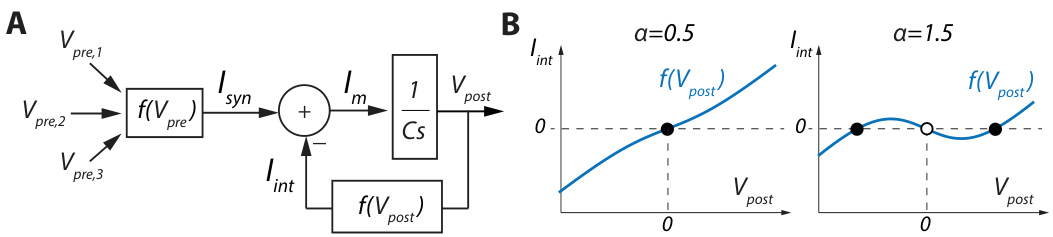
Figure 1: A. One timescale control diagram of a neuron. B. Plot of the function ${I_{i n t}=V_{p o s t}-}$ $\alpha\operatorname{tanh}(V_{p o s t})$ for two different values of $\alpha$ . Full dots correspond to stable states, empty dots to unstable states.
图 1: A. 神经元单时间尺度控制图。B. 函数 ${I_{i n t}=V_{p o s t}-}$ $\alpha\operatorname{tanh}(V_{p o s t})$ 在两种不同 $\alpha$ 值下的曲线图。实心圆点对应稳定状态,空心圆点对应不稳定状态。
The switch between mono stability and bi stability is achieved by shaping the nonlinear function ${\cal I}_ {i n t}=f(V_{p o s t})$ (Figure 1B). The neuron is monostable when $\bar{f}(V_{p o s t})$ is monotonic of positive slope (Figure 1B, left). Its only stable state corresponds to the voltage at which $I_{i n t}=0$ in the absence of synaptic inputs (full dot). The neuron switch to bi stability through the creation of a local region of negative slope in $f(V_{p o s t})$ (Figure 1B, left). Its two stable states correspond to the voltages at which $I_{i n t}=0$ with positive slope (full dots), separated by an unstable state where $I_{i n t}=0$ with negative slope (empty dot). The local region of negative slope corresponds to a local positive feedback where the membrane voltage is unstable.
单稳态和双稳态之间的切换是通过塑造非线性函数 ${\cal I}_ {i n t}=f(V_{p o s t})$ 实现的 (图 1B)。当 $\bar{f}(V_{p o s t})$ 具有正斜率的单调性时,神经元处于单稳态 (图 1B 左)。其唯一稳定状态对应于无突触输入时 $I_{i n t}=0$ 的电压值 (实心圆点)。通过在 $f(V_{p o s t})$ 中创建负斜率局部区域,神经元切换为双稳态 (图 1B 左)。其两个稳定状态对应于 $I_{i n t}=0$ 且斜率为正的电压值 (实心圆点),中间被一个 $I_{i n t}=0$ 且斜率为负的不稳定状态隔开 (空心圆点)。负斜率局部区域对应膜电压不稳定的局部正反馈。
In biological neurons, a local positive feedback is provided by regenerative gating, such as sodium and calcium channel activation or potassium channel in activation ([18, 19]). The switch from mono stability to bi stability can therefore be controlled by tuning ion channel density. This property can be emulated in electrical circuits by combining trans conductance amplifiers to create the function
在生物神经元中,局部正反馈通过再生门控提供,例如钠和钙通道激活或钾通道失活 ([18, 19])。因此,通过调节离子通道密度可以控制从单稳态到双稳态的切换。这一特性可通过结合跨导放大器来创建功能电路进行模拟。
$$
I_{i n t}=V_{p o s t}-\alpha\operatorname{tanh}(V_{p o s t}),
$$
$$
I_{i n t}=V_{p o s t}-\alpha\operatorname{tanh}(V_{p o s t}),
$$
where the switch from mono stability to bi stability is controlled by a single parameter $\alpha$ ([20]). $\alpha$ models the effect of sodium or calcium channel activation, which tunes the local slope of the function, hence the local gain of the feedback loop (Figure 1B). For $\alpha\in]0,1]$ , which models a low sodium or calcium channel density, the function is monotonic, leading to mono stability (Figure 1B, left). For $\alpha\in]1,+\infty[$ , which models a high sodium or calcium channel density, a region of negative slope is created around $V_{p o s t}=0$ , and the neuron becomes bistable (Figure 1B, right). This bistability leads to never-fading memory, as in the absence of significant input perturbation the system will remain indefinitely in one of the two stable states depending on the input history.
其中从单稳态到双稳态的切换由单一参数 $\alpha$ 控制 ([20])。$\alpha$ 模拟了钠或钙通道激活的效果,调节了函数的局部斜率,从而调节反馈环路的局部增益 (图 1B)。对于 $\alpha\in]0,1]$ (模拟低钠或钙通道密度的情况),函数是单调的,导致单稳态 (图 1B,左)。对于 $\alpha\in]1,+\infty[$ (模拟高钠或钙通道密度的情况),在 $V_{post}=0$ 附近会产生一个负斜率区域,神经元变为双稳态 (图 1B,右)。这种双稳态会导致永不消逝的记忆,因为在没有显著输入扰动的情况下,系统会根据输入历史无限期地保持在两个稳定状态之一。
Neuronal bi stability can therefore be modeled by a simple feedback system whose dynamics is tuned by a single feedback parameter $\alpha$ . This parameter can switch between mono stability and bi stability by tuning the shape of the feedback function $f(V_{p o s t})$ , whereas neuron convergence dynamics is controlled by a single feed forward parameter $C$ . In biological neurons, both these parameters can be modified dynamically by other neurons via a mechanism called neuro modulation, providing a dynamic, controllable memory at the cellular level. The key challenge is to find an appropriate mathematical representation of this mechanism to be efficiently used in artificial neural networks, and, more particularly, in RNNs.
因此,神经元双稳态可以通过一个简单的反馈系统建模,其动力学由单一反馈参数 $\alpha$ 调节。该参数可通过调整反馈函数 $f(V_{post})$ 的形状在单稳态与双稳态之间切换,而神经元收敛动力学则由单一前馈参数 $C$ 控制。在生物神经元中,这两个参数均可通过神经调制机制被其他神经元动态修改,从而在细胞层面实现动态可控的记忆功能。关键挑战在于找到该机制的合适数学表征,以高效应用于人工神经网络,尤其是循环神经网络 (RNN) 中。
4 Cellular memory, bi stability and neuro modulation in RNNs
4 RNN中的细胞记忆、双稳态和神经调节
The bistable recurrent cell (BRC) To model controllable bi stability in RNNs, we start by drawing two main comparisons between the feedback structure Figure 1A and the GRU equations (Equation 2). First, we note that the reset gate $r$ has a role that is similar to the one played by the feedback gain $\alpha$ in Equation 3. In GRU equations, $r$ is the output of a sigmoid function, which implies $r\in]0,1[$ [. These possible values for $r$ correspond to negative feedback only, which does not allow for bi stability. The update gate $z$ , on the other hand, has a role similar to that of the membrane capacitance $C$ . Second, one can see through the matrix multiplications $W_{z}\mathbf{h}_ {t-1}$ , $W_{r}\mathbf{h}_ {t-1}$ and $W_{h}\mathbf{h}_ {t-1}$ that each cell uses the internal state of other neurons to compute its own state without going through synaptic connections. In biological neurons, the intrinsic dynamics defined by $I_{i n t}$ is constrained to only depend on its own state $V_{p o s t}$ , and the influence of other neurons comes only through the synaptic compartment $(I_{s y n})$ , or through neuro modulation.
双稳态循环单元 (BRC) 为在循环神经网络中建立可控双稳态模型,我们首先对反馈结构图1A和GRU方程(式2)进行两项主要比较。首先,我们发现重置门$r$的作用类似于式3中的反馈增益$\alpha$。在GRU方程中,$r$是sigmoid函数的输出,这意味着$r\in]0,1[$。$r$的这些可能取值仅对应负反馈,无法实现双稳态。而更新门$z$的作用则类似于膜电容$C$。其次,通过矩阵乘法$W_{z}\mathbf{h}_ {t-1}$、$W_{r}\mathbf{h}_ {t-1}$和$W_{h}\mathbf{h}_ {t-1}$可以看出,每个单元都使用其他神经元的内部状态来计算自身状态,而无需经过突触连接。在生物神经元中,由$I_{int}$定义的内在动力学仅依赖于其自身状态$V_{post}$,其他神经元的影响仅通过突触区$(I_{syn})$或神经调节实现。
To enforce this cellular feedback constraint in GRU equations and to endow them with bi stability, we propose to update $h_{t}$ as follows:
为了在GRU方程中实施这种细胞反馈约束并赋予其双稳态特性,我们提出按以下方式更新 $h_{t}$:
$$
\mathbf{h}_ {t}=\mathbf{c}_ {t}\odot\mathbf{h}_ {t-1}+\left(1-\mathbf{c}_ {t}\right)\odot\operatorname{tanh}(U\mathbf{x}_ {t}+\mathbf{a}_ {t}\odot\mathbf{h}_{t-1})
$$
$$
\mathbf{h}_ {t}=\mathbf{c}_ {t}\odot\mathbf{h}_ {t-1}+\left(1-\mathbf{c}_ {t}\right)\odot\operatorname{tanh}(U\mathbf{x}_ {t}+\mathbf{a}_ {t}\odot\mathbf{h}_{t-1})
$$
where $\mathbf{a}_ {t}=1+\operatorname{tanh}(U_{a}\mathbf{x}_ {t}+\mathbf{w}_ {a}\odot\mathbf{h}_ {t-1})$ and $\mathbf{c}_ {t}=\sigma(U_{c}\mathbf{x}_ {t}+\mathbf{w}_ {c}\odot\mathbf{h}_ {t-1})$ . $\mathbf{a}_ {t}$ corresponds to the feedback parameter $\alpha$ , with ${\mathbf a}_ {t}\in]0,2[$ [. $\mathbf{c}_{t}$ corresponds to the update gate in GRU and plays the role of the membrane capacitance $C$ , determining the convergence dynamics of the neuron. We call this updated cell the bistable recurrent cell (BRC).
其中 $\mathbf{a}_ {t}=1+\operatorname{tanh}(U_{a}\mathbf{x}_ {t}+\mathbf{w}_ {a}\odot\mathbf{h}_ {t-1})$ ,且 $\mathbf{c}_ {t}=\sigma(U_{c}\mathbf{x}_ {t}+\mathbf{w}_ {c}\odot\mathbf{h}_ {t-1})$ 。$\mathbf{a}_ {t}$ 对应反馈参数 $\alpha$ ,其中 ${\mathbf a}_ {t}\in]0,2[$ 。$\mathbf{c}_{t}$ 对应 GRU 中的更新门,并起到膜电容 $C$ 的作用,决定神经元的收敛动态特性。我们将这个更新后的单元称为双稳态循环单元 (BRC)。
The main differences between a BRC and a GRU are twofold. First, each neuron has its own internal state $\mathbf{h}_ {t}$ that is not directly affected by the internal state of the other neurons. Indeed, due to the four instances of $\mathbf{h}_ {t-1}$ coming from Hadamard products, the only temporal connections existing in layers of BRC are from neurons to themselves. This enforces the memory to be only cellular. Second, the feedback parameter $\mathbf{a}_{t}$ is allowed to take a value in the range $|0,2[$ rather than $]0,1[$ . This allows the cell to switch between mono stability $(a\leq1)$ and bi stability $\left(a>1\right)$ ) (Figure 2A,B). The proof of this switch is provided in Appendix A.
BRC与GRU的主要区别有两点。首先,每个神经元都有独立的内部状态$\mathbf{h}_ {t}$,不受其他神经元内部状态的直接影响。由于Hadamard积引入的四个$\mathbf{h}_ {t-1}$实例,BRC层中仅存在神经元自身的时序连接,这强制实现了细胞级记忆。其次,反馈参数$\mathbf{a}_{t}$的取值范围扩展为$|0,2[$而非$]0,1[$,使细胞能在单稳态$(a\leq1)$和双稳态$\left(a>1\right)$之间切换(图2A,B)。该切换机制的证明详见附录A。
It is important to note that the parameters $\mathbf{a}_ {t}$ and $\mathbf{c}_ {t}$ are dynamic. $\mathbf{a}_ {t}$ and $\mathbf{c}_{t}$ are neuro modulated by the previous layer, that is, their value depends on the output of other neurons. Tests were carried with a and c as parameters learned by stochastic gradient descent, which resulted in lack of represent at ional power, leading to the need for neuro modulation. This neuro modulation scheme was the most evident as it maintains the cellular memory constraint and leads to the most similar update rule with respect to standard recurrent cells (Equation 2). However, as will be discussed later, other neuro modulation schemes can be thought of.
需要注意的是,参数 $\mathbf{a}_ {t}$ 和 $\mathbf{c}_ {t}$ 是动态的。$\mathbf{a}_ {t}$ 和 $\mathbf{c}_{t}$ 受到上一层的神经调节 (neuro modulation) ,即它们的值取决于其他神经元的输出。实验曾尝试将a和c作为通过随机梯度下降 (stochastic gradient descent) 学习的参数,但会导致表征能力不足,从而需要引入神经调节。这种神经调节方案最为明显,因为它保持了细胞记忆约束,并产生了与标准循环单元最相似的更新规则 (Equation 2) 。不过,后文将讨论其他可能的神经调节方案。
Likewise, from a neuroscience perspective, $\mathbf{a}_ {t}$ could well be greater than 2. Limiting the range of $\mathbf{a}_ {t}$ to $|0,2[$ was made for numerical stability and for symmetry between the range of bistable and monostable neurons. We argue that this is not an issue as, for a value of $\mathbf{a}_{t}$ greater than 1.5, the dynamics of the neurons become very similar (as suggested in Figure 2A).
同样,从神经科学的角度来看,$\mathbf{a}_ {t}$ 完全可以大于2。将 $\mathbf{a}_ {t}$ 的范围限制在 $|0,2[$ 是为了数值稳定性以及双稳态和单稳态神经元范围之间的对称性。我们认为这不是问题,因为当 $\mathbf{a}_{t}$ 的值大于1.5时,神经元的动态行为变得非常相似(如图 2A 所示)。
Figure 2C shows the dynamics of a BRC with respect to $a_{t}$ and $c_{t}$ . For $a_{t}<1$ , the cell exhibits a classical monostable behavior, relaxing to the 0 stable state in the absence of inputs (blue curves in Figure 2C). On the other hand, a bistable behavior can be observed for $a_{t}>1$ : the cells can either stabilize on an upper stable state or a lower stable state depending on past inputs (red curves in Figure 2C). Since these upper and lower stable states do not correspond to an $h_{t}$ which is equal to 0, they can be associated with cellular memory that never fades over time. Furthermore, Figure 2 also illustrates that neuron convergence dynamics depend on the value of $c$ .
图 2C 展示了 BRC 相对于 $a_{t}$ 和 $c_{t}$ 的动态变化。当 $a_{t}<1$ 时,细胞表现出经典的单调稳定行为,在没有输入的情况下会弛豫到 0 稳定状态 (图 2C 中的蓝色曲线)。另一方面,当 $a_{t}>1$ 时可以观察到双稳态行为:细胞会根据过去的输入稳定在上稳定状态或下稳定状态 (图 2C 中的红色曲线)。由于这些上稳定状态和下稳定状态不对应于 $h_{t}$ 等于 0 的情况,因此它们可以与永不随时间消退的细胞记忆相关联。此外,图 2 还说明了神经元收敛动态取决于 $c$ 的值。
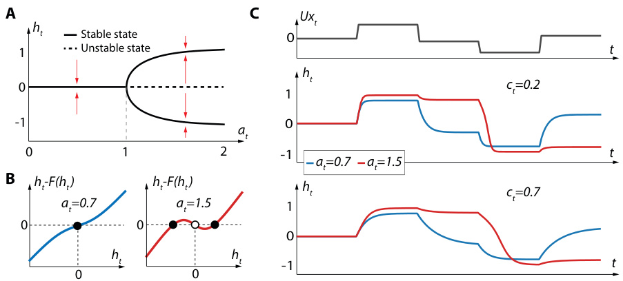
Figure 2: A. Bifurcation diagram of Equation 4 for $U\mathbf{x}_ {t}=0$ . B. Plots of the function $h_{t}-F(h_{t})$ for two values of $a_{t}$ , where $\bar{F(h_{t})}=c_{t}\bar{h}{t}+(1-c{t})\operatorname{tanh}(a_{t}h_{t})$ is the right hand side of Equation 4 with $x_{t}=0$ . Full dots correspond to stable states, empty dots to unstable states. C. Response of BRC to an input time-series for different values of $a_{t}$ and $c_{t}$ .
图 2: A. 当 $U\mathbf{x}_ {t}=0$ 时方程 4 的分岔图。B. 函数 $h_{t}-F(h_{t})$ 在两种 $a_{t}$ 值下的曲线图,其中 $\bar{F(h_{t})}=c_{t}\bar{h}{t}+(1-c{t})\operatorname{tanh}(a_{t}h_{t})$ 是方程 4 在 $x_{t}=0$ 时的右侧表达式。实心点表示稳定状态,空心点表示不稳定状态。C. BRC 在不同 $a_{t}$ 和 $c_{t}$ 值下对输入时间序列的响应。
The re currently neuro modulated bistable recurrent cell (nBRC) To further improve the performance of BRC, one can relax the cellular memory constraint. By creating a dependency of $a_{t}$ and $c_{t}$ on the output of other neurons of the layer, one can build a kind of recurrent layer-wise neuro modulation. We refer to this modified version of a BRC as an nBRC, standing for re currently neuro modulated BRC. The update rule for the nBRC is the same as for BRC, and follows Equation 4. The difference comes in the computation of $a_{t}$ and $c_{t}$ , which are neuro modulated as follows:
目前神经调制的双稳态循环单元 (nBRC)
为了进一步提升BRC的性能,可以放宽单元记忆约束。通过让$a_{t}$和$c_{t}$依赖于该层其他神经元的输出,可以构建一种循环层间神经调制机制。我们将这种改进版的BRC称为nBRC,意为"循环神经调制的BRC"。nBRC的更新规则与BRC相同,遵循公式4。差异体现在$a_{t}$和$c_{t}$的计算上,其神经调制方式如下:

The update rule of nBRCs being that of BRCs (Equation 4), bistable properties are maintained and hence the possibility of a cellular memory that does not fade over time. However, the new recurrent neuro modulation scheme adds a type of network memory on top of the cellular memory. This recurrent neuro modulation scheme brings the update rule even closer to standard GRU. This is highlighted when comparing Equation 2 and Equation 4 with parameters neuro modulated following Equation 5. We stress that, as opposed to GRUs, bi stability is still ensured through $a_{t}$ belonging to $|0,2[$ . A relaxed cellular memory constraint is also ensured, as each neuron past state $h_{t-1}$ only directly influences its own current state and not the state of other neurons of the layer (Hadamard product on the $\mathbf{h}_ {t}$ update in Equation 4). This is important for numerical stability as the introduction of a cellular positive feedback for bi stability leads to global instability if the update is computed using other neurons states directly (as it is done in the classical GRU update, see the matrix multiplication $W_{h}\mathbf{h}_{t-1}$ in Equation 2).
nBRC的更新规则与BRC相同(公式4),因此保留了双稳态特性,从而实现了不会随时间消退的细胞记忆。然而,新的循环神经调节机制在细胞记忆基础上新增了网络记忆功能。这种循环神经调节机制使更新规则更接近标准GRU结构,通过对比公式2与采用公式5进行神经调节的公式4即可看出这一特点。需要强调的是,与GRU不同,双稳态仍通过$a_{t}$属于$|0,2[$区间得以保证。同时实现了宽松的细胞记忆约束——每个神经元过去状态$h_{t-1}$仅直接影响自身当前状态,而不会直接影响同层其他神经元状态(见公式4中$\mathbf{h}_ {t}$更新的Hadamard积)。这对数值稳定性至关重要:若直接采用其他神经元状态进行计算(如经典GRU更新中的矩阵乘法$W_{h}\mathbf{h}_{t-1}$见公式2),为维持双稳态引入的细胞正反馈会导致全局不稳定性。
Finally, let us note that to be consistent with the biological model presented in Section 3, Equation 5 should be interpreted as a way to represent a neuro modulation mechanism of a neuron by those from its own layer and the layer that precedes. Hence, the possible analogy between gates $z$ and $r$ in GRUs and neuro modulation. In this respect, studying the introduction of new types of gates based on more biological plausible neuro modulation architectures would certainly be interesting.
最后,我们注意到,为了与第3节中提出的生物模型保持一致,方程5应被解释为一种表示神经元通过来自自身层和前一层神经元的神经调节机制的方式。因此,GRU中的门控 $z$ 和 $r$ 与神经调节之间可能存在类比。在这方面,研究基于更具生物学合理性的神经调节架构引入新型门控机制无疑会非常有趣。
5 Analysis of BRC and nBRC performance
5 BRC 和 nBRC 性能分析
To demonstrate the performances of BRCs and nBRCs with respect to standard GRUs and LSTMs, we tackle three problems. The first is a one-dimensional toy problem, the second is a twodimensional denoising problem and the third is the sequential MNIST problem. The supervised setting used is the same for all three benchmarks. The network is presented with a time-series and is asked to output a prediction (regression for the first two benchmarks and classification for the third) after having received the last element of the time-series $\mathbf{x}_{T}$ . We show that the introduction of bi stability in recurrent cells is especially useful for datasets in which only sparse time-series are available. In this section, we also take a look at the dynamics inside the BRC neurons in the context of the denoising benchmark and show that bi stability is heavily used by the neural network.
为了展示BRC和nBRC相对于标准GRU和LSTM的性能表现,我们研究了三个问题。第一个是一维玩具问题,第二个是二维去噪问题,第三个是顺序MNIST问题。这三个基准测试采用相同的监督设置:网络接收一个时间序列,并在接收到该序列的最后一个元素$\mathbf{x}_{T}$后输出预测结果(前两个基准测试为回归任务,第三个为分类任务)。我们证明,在循环单元中引入双稳态特性对于稀疏时间序列数据集特别有效。本节还通过去噪基准测试分析了BRC神经元内部的动态特性,表明神经网络充分运用了双稳态机制。
| T | BRC | nBRC | GRU | LSTM |
| 5 | 0.0157± 0.0124 | 0.0028± 0.0023 | 0.0019 ± 0.0011 | 0.0016± 0.0009 |
| 50 | 0.0142± 0.0081 | 0.0009 ± 0.0006 | 0.0004±0.0003 | 0.9919±0.0012 |
| 100 | 0.0046±0.0002 | 0.0006± 0.0001 | 0.0097± 0.006 | 1.0354± 0.0416 |
| 300 | 0.0013±0.0008 | 0.0007 ± 0.0002 | 0.6743± 0.4761 | 0.9989 ± 0.0170 |
| 600 | 0.1581±0.1574 | 0.0005±0.0001 | 0.9934±0.0182 | 0.9989±0.0162 |
| T | BRC | nBRC | GRU | LSTM |
|---|---|---|---|---|
| 5 | 0.0157±0.0124 | 0.0028±0.0023 | 0.0019±0.0011 | 0.0016±0.0009 |
| 50 | 0.0142±0.0081 | 0.0009±0.0006 | 0.0004±0.0003 | 0.9919±0.0012 |
| 100 | 0.0046±0.0002 | 0.0006±0.0001 | 0.0097±0.006 | 1.0354±0.0416 |
| 300 | 0.0013±0.0008 | 0.0007±0.0002 | 0.6743±0.4761 | 0.9989±0.0170 |
| 600 | 0.1581±0.1574 | 0.0005±0.0001 | 0.9934±0.0182 | 0.9989±0.0162 |
Table 1: Mean square error on test set after 30000 gradient descent iterations of different architectures on the copy first input benchmark. Results are shown for different values of $T$ .
表 1: 不同架构在复制首输入基准任务上经过30000次梯度下降迭代后的测试集均方误差。结果展示了不同 $T$ 值下的表现。

Figure 3: Evolution of the average mean-square error ( $\pm$ standard deviation) over three runs on the copy input benchmark for GRU and BRC and for different values of $T$ .
图 3: GRU和BRC在复制输入基准测试中,针对不同$T$值时平均均方误差( $\pm$ 标准差)在三轮运行中的演变情况。
5.1 Results
5.1 结果
For the first two problems, training sets comprise 45000 samples and performances are evaluated on test sets generated with 50000 samples. For the MNIST benchmark, the standard train and test sets are used. All averages and standard deviations reported were computed over three different seeds. We found that there were very little variations in between runs, and thus believe that three runs are enough to capture the performance of the different architectures. For benchmark 1, networks are composed of two recurrent layers of 100 neurons each whereas for benchmark 2 and 3, networks are composed of four recurrent layers of 100 neurons each. Different recurrent cells are always tested on similar networks (i.e. same number of layers/neurons). We used the tensorflow ([21]) implementation of GRUs and LSTMs. Finally, the ADAM optimizer with a learning rate of $1e^{-3}$ is used for training all networks, with a mini-batch size of 100. The source code for carrying out the experiments is available at https://github.com/nvecoven/BRC.
对于前两个问题,训练集包含45000个样本,性能评估基于50000个样本生成的测试集。MNIST基准测试则使用标准训练集和测试集。所有报告的均值和标准差均基于三个不同随机种子计算得出。我们发现不同运行间的差异极小,因此认为三次运行足以反映各架构的性能表现。在基准测试1中,网络由两个各含100个神经元的循环层组成;基准测试2和3则采用四个各含100个神经元的循环层。不同循环单元始终在结构相似的网络上测试(即相同层数/神经元数)。我们使用了tensorflow ([21])实现的GRU和LSTM,所有网络均采用学习率为$1e^{-3}$的ADAM优化器进行训练,最小批处理量为100。实验源代码详见https://github.com/nvecoven/BRC。
Copy first input benchmark In this benchmark, the network is presented with a one-dimensional time-series of $T$ time-steps where $x_{t}\sim\mathcal{N}(0,1)$ , $\forall t\in T$ . After receiving $x_{T}$ , the network output value should approximate $x_{0}$ , a task that is well suited for capturing their capacity to learn long temporal dependencies if $T$ is large. Note that this benchmark also requires the ability to filter irrelevant signals as, after time-step 0, the networks are continuously presented with noisy inputs that they must learn to ignore. The mean square error on the test set is shown for different values of $T$ in Table 1. For smaller values of $T$ , all recurrent cells achieve similar performances. The advantage of using bistable recurrent cells appears when $T$ becomes large (Figure 3). Indeed, when $T$ is equal to 600, only networks made of bistable cells are capable of outperforming random guessing threshold (which would be equal to 1 in this setting 1).
复制首个输入基准测试
在此基准测试中,网络接收一个长度为 $T$ 的一维时间序列,其中 $x_{t}\sim\mathcal{N}(0,1)$,$\forall t\in T$。接收到 $x_{T}$ 后,网络输出值应逼近 $x_{0}$。若 $T$ 值较大,该任务能有效衡量网络学习长时依赖关系的能力。需注意的是,此基准测试还要求网络具备过滤无关信号的能力,因为在时间步0之后,网络会持续接收到必须学会忽略的噪声输入。
表1展示了不同 $T$ 值下测试集的均方误差。当 $T$ 值较小时,所有循环单元表现相近。而 $T$ 值较大时(图3),双稳态循环单元的优势开始显现。具体而言,当 $T$ 达到600时,仅由双稳态单元构成的网络能够超越随机猜测阈值(本设定中该阈值为1)。
Denoising benchmark The copy input benchmark is interesting as a means to highlight the memorisation capacity of the recurrent neural network, but it does not tackle its ability to successfully exploit complex relationships between different elements of the input signal to predict the output. In the denoising benchmark, the network is presented with a two-dimensional time-series of $T$ time-steps. Five different time-steps $t_{1},\ldots,t_{5}$ are sampled uniformly in ${0,\dots,T-N}$ with
去噪基准测试
复制输入基准测试作为一种突显循环神经网络记忆能力的手段很有趣,但它并未解决网络能否成功利用输入信号中不同元素间的复杂关系来预测输出的能力。在去噪基准测试中,网络接收一个包含 $T$ 个时间步的二维时间序列。从 ${0,\dots,T-N}$ 中均匀采样五个不同时间步 $t_{1},\ldots,t_{5}$,并满足...
| N | BRC | nBRC | GRU | LSTM |
| 0 | 0.0014± 0.0001 | 0.0006 ± 0.0001 | 0.0001±0.0001 | 0.0003±0.0002 |
| 200 | 0.0032±0.0015 | 0.0013±0.0006 | 1.0571±0.0452 | 0.9878±0.0052 |
| N | BRC | nBRC | GRU | LSTM |
|---|---|---|---|---|
| 0 | 0.0014±0.0001 | 0.0006±0.0001 | 0.0001±0.0001 | 0.0003±0.0002 |
| 200 | 0.0032±0.0015 | 0.0013±0.0006 | 1.0571±0.0452 | 0.9878±0.0052 |
Table 2: Mean square error on test set after 30000 gradient descent iterations of different architectures on the denoising benchmark. Results are shown with and without constraint on the location of relevant inputs. Relevant inputs cannot appear in the $N$ last time-steps, that is ${\bf x}_{t}[1]=-1,\forall t>$ $(T-N)$ . In this experiment, results were obtained with $T=400$ .
表 2: 不同架构在去噪基准任务上经过30000次梯度下降迭代后的测试集均方误差。结果展示了是否对相关输入位置施加约束的对比情况。相关输入不允许出现在最后 $N$ 个时间步中,即 ${\bf x}_{t}[1]=-1,\forall t>$ $(T-N)$ 。本实验中采用 $T=400$ 进行测试。
| BRC | nBRC | GRU | LSTM |
| 0.0010±0.0001 | 0.0001± 0.0001 | 0.0373±0.00371 | 0.3323±0.4635 |
| BRC | nBRC | GRU | LSTM |
|---|---|---|---|
| 0.0010±0.0001 | 0.0001±0.0001 | 0.0373±0.00371 | 0.3323±0.4635 |
Table 3: Mean square error on test set after 30000 gradient descent iterations of different architectures on the modified copy input benchmark.
表 3: 不同架构在修改版复制输入基准测试上经过30000次梯度下降迭代后的测试集均方误差
$N\in{0,\ldots,T-5}$ and are communicated to the network through the first dimension of the timeseries by setting $\mathbf{x}_ {t}[1]=0$ if $t\in[t_{1},\ldots,t_{5}]$ , ${\mathbf x}_ {t}[1]=1$ if $t=T$ and ${\mathbf x}_{t}[1]=-1$ otherwise.
$N\in{0,\ldots,T-5}$ 并通过时间序列的第一个维度传递至网络,设定规则为:当 $t\in[t_{1},\ldots,t_{5}]$ 时 $\mathbf{x}_ {t}[1]=0$,当 $t=T$ 时 ${\mathbf x}_ {t}[1]=1$,其余情况 ${\mathbf x}_{t}[1]=-1$。
Note that this dimension is also used to notify the network that the end of the time-series is reached (and thus, that the network should output its prediction). The second dimension is a data-stream, generated as for the copy first input benchmark, that is $\mathbf{x}_ {t}[2]\sim\mathcal{N}(0,1),\forall t\in T$ . At time-step $T$ , the network is asked to output $[\bar{\mathbf{x}}_ {t_{1}}[2],\ldots,\mathbf{x}_ {t_{5}}[2]]$ . The mean squared error is averaged over the 5 values. That is, the error on the prediction is equal to i5=1 (xti [2]5−O[i]) with $\mathbf{O}$ the output of the neural network. Note that the parameter $N$ controls the lPength of the forgetting period as it forces the relevant inputs to be in the first $T-N$ time-steps. This ensures that $t_{x}<T-N$ , $\forall x\in{1,\ldots,5}$ . As one can see in Table 2 (generated with $T=200$ and two different values of $N$ ), for $N=200$ , GRUs and LSTMs are unable to exceed random guessing (mean square error of 1) whereas BRC and nBRC performances are virtually unimpacted. Also, Table 2 provides a very important observation. GRUs and LSTMs are, in fact, able to learn long-term dependencies, as they achieve extremely good performances when $N=0$ . In fact, all the samples generated when $N=200$ could also be generated when $N=0$ , meaning that with the right parameters, the GRUs and LSTMs network could achieve good predictive performances on such samples. However, our results show that GRUs and LSTMs are unable to learn those parameters when the datasets are only composed of such samples. That is, GRUs and LSTMs need training datasets with some samples for which the memory required is quite short to learn efficiently, and allow for learning the samples for which the temporal structure is longer. Bistable cells on the other hand are not susceptible to this caveat.
请注意,该维度还用于通知网络时间序列已结束(因此网络应输出其预测)。第二个维度是一个数据流,其生成方式与复制第一个输入基准相同,即 $\mathbf{x}_ {t}[2]\sim\mathcal{N}(0,1),\forall t\in T$。在时间步 $T$,网络被要求输出 $[\bar{\mathbf{x}}_ {t_{1}}[2],\ldots,\mathbf{x}_ {t_{5}}[2]]$。均方误差在这5个值上取平均。也就是说,预测误差等于 i5=1 (xti [2]5−O[i]),其中 $\mathbf{O}$ 是神经网络的输出。注意,参数 $N$ 控制遗忘周期的长度,因为它强制相关输入必须位于前 $T-N$ 个时间步内。这确保了 $t_{x}<T-N$,$\forall x\in{1,\ldots,5}$。如表2所示(使用 $T=200$ 和两个不同的 $N$ 值生成),当 $N=200$ 时,GRU和LSTM无法超越随机猜测(均方误差为1),而BRC和nBRC的性能几乎不受影响。此外,表2提供了一个非常重要的观察结果。事实上,GRU和LSTM能够学习长期依赖关系,因为当 $N=0$ 时它们表现出极佳的性能。实际上,$N=200$ 时生成的所有样本也可以在 $N=0$ 时生成,这意味着只要参数合适,GRU和LSTM网络在此类样本上也能取得良好的预测性能。然而,我们的结果表明,当数据集仅由此类样本组成时,GRU和LSTM无法学习这些参数。也就是说,GRU和LSTM需要训练数据集中包含一些所需记忆较短的样本才能高效学习,并进而学习时间结构较长的样本。而双稳态单元则不受此限制影响。
To further highlight this behavior, we design another benchmark that is a variant of the copy input benchmark. In this benchmark, the network is presented with a one-dimensional time-series of length $T=600$ where $x_{t}~=~0$ , $\forall t\in T\backslash t_{1}$ and $\boldsymbol x_{t_{1}}\sim\mathcal N(\boldsymbol0,\boldsymbol1)$ , with $t_{1}$ chosen uniformly in ${0,\ldots,599}$ . The network is tasked to output $x_{t_{1}}$ . Table 3 shows that, using this training scenario, GRUs are capable of achieving a low MSE (around 0.04) on the test set used for the original copy input benchmark in which all the $T=600$ . This was not the case in Table 1 (MSE around 1.0 for $T=600,$ ), when trained on a datasets for which all the samples require a 600 time-step-long dependency. On the other hand, the performance of BRC and nBRC peaked in this scenario.
为了进一步突显这一行为,我们设计了另一个基准测试,它是复制输入基准的一个变体。在该基准中,网络接收一个长度为 $T=600$ 的一维时间序列,其中 $x_{t}~=~0$,$\forall t\in T\backslash t_{1}$,且 $\boldsymbol x_{t_{1}}\sim\mathcal N(\boldsymbol0,\boldsymbol1)$,其中 $t_{1}$ 在 ${0,\ldots,599}$ 中均匀随机选择。网络的任务是输出 $x_{t_{1}}$。表 3 显示,使用这种训练场景,GRU 能够在原始复制输入基准的测试集上实现较低的均方误差 (MSE)(约为 0.04),该测试集中所有 $T=600$。而在表 1 中(当训练数据集中所有样本都需要 600 个时间步长的依赖关系时,$T=600$ 的 MSE 约为 1.0)情况并非如此。另一方面,BRC 和 nBRC 在此场景中的性能达到了峰值。
Sequential MNIST In this benchmark, the network is presented with the MNIST images, shown pixel by pixel as a time-series. MNIST images are made of 1024 pixels (32 by 32), showing that BRC and nBRC can learn dynamics over thousands of time-steps. Similar to both previous benchmarks, we add $n_{b l a c k}$ time-steps of black pixels at the end of the time-series to add a forgetting period. Results are shown in Table 4 for two values of $n_{b l a c k}$ , and are consistent with what has been observed in both previous benchmarks.
顺序MNIST
在此基准测试中,网络接收MNIST图像数据,这些图像以逐像素的时间序列形式呈现。MNIST图像由1024个像素(32×32)组成,表明BRC和nBRC能够在数千个时间步长上学习动态特征。与前述两个基准测试类似,我们在时间序列末尾添加 $n_{b l a c k}$ 个黑色像素时间步长以引入遗忘周期。表4展示了两种 $n_{b l a c k}$ 值的测试结果,该结果与前述两个基准测试的观测结论一致。
表4:
5.2 Analysis of BRC dynamic behavior
5.2 BRC动态行为分析
Until now, we have looked at the learning performances of bistable recurrent cells. It is however interesting to take a deeper look at the dynamics of such cells to understand whether or not bi stability
迄今为止,我们已研究了双稳态循环单元的学习性能。然而,更深入地观察此类单元的动力学特性,以理解双稳态是否...
| nblack | BRC | nBRC | GRU | LSTM |
| 0 | 0.9697±0.0020 | 0.9601 ± 0.0032 | 0.9880±0.0014 | 0.9651± 0.0023 |
| 300 | 0.9760±0.0015 | 0.9608±0.0109 | 0.1081±0.0053 | 0.1124±0.0013 |
| nblack | BRC | nBRC | GRU | LSTM |
|---|---|---|---|---|
| 0 | 0.9697±0.0020 | 0.9601 ± 0.0032 | 0.9880±0.0014 | 0.9651± 0.0023 |
| 300 | 0.9760±0.0015 | 0.9608±0.0109 | 0.1081±0.0053 | 0.1124±0.0013 |
Table 4: Accuracy on MNIST test set after 30000 gradient descent iterations on different architectures on the MNIST benchmark. Images are fed to the recurrent network pixel by pixel. Results are shown for MNIST images with $n_{b l a c k}$ black pixels appended to the image.
表 4: 在MNIST基准测试中,不同架构经过30000次梯度下降迭代后在MNIST测试集上的准确率。图像以逐像素方式输入循环网络。结果显示为在图像后附加 $n_{black}$ 个黑色像素的MNIST图像。

Figure 4: Representation of the BRC parameters, per layer, of a recurrent neural network (with 4 layers of 100 neurons each), when shown a time-series of the denoising benchmark $\mathit{T}=400$ , $N=0$ ). Layer numbering increases as layers get deeper (i.e. layer i corresponds to the ith layer of the network). The 5 time-steps at which a relevant input is shown to the model are clearly distinguishable by the behaviour of those measures alone.
图 4: 循环神经网络(包含4层、每层100个神经元)在去噪基准时间序列($\mathit{T}=400$, $N=0$)中每层的BRC参数表示。层编号随深度增加(即第i层对应网络的第i层)。仅通过这些测量指标的行为即可清晰区分模型接收相关输入的5个时间步。
is used by the network. To this end, we pick a random time-series from the denoising benchmark and analyse some properties of $a_{t}$ and $c_{t}$ . Figure 4 shows the proportion of bistable cells per layer and the average value of $e_{t}$ per layer. The dynamics of the parameters show that they are well used by the network, and three main observations owe to be made. First, as relevant inputs are shown to the network, the proportion of bistable neurons tends to increase in layers 2 and 3, effectively storing information and thus confirming the interest of introducing bi stability for long-term memory. As more information needs to be stored, the network leverages the power of bi stability by increasing the number of bistable neurons. Second, as relevant inputs are shown to the network, the average value $c_{t}$ tends to increase in layer 3, effectively making the network less and less sensitive to new inputs. Third, one can observe a transition regime when a relevant input is shown. Indeed, there is a high decrease in the average value of $c_{t}$ , effectively making the network extremely sensitive to the current input, which allows for its efficient memorization.
网络使用了这一机制。为此,我们从去噪基准测试中随机选取一个时间序列,分析了 $a_{t}$ 和 $c_{t}$ 的若干特性。图4展示了每层双稳态细胞的比例以及每层 $e_{t}$ 的平均值。参数动态表明网络对其进行了有效利用,可得出三个主要观察结论:首先,当网络接收相关输入时,第2层和第3层的双稳态神经元比例会上升,有效存储信息,从而证实了引入双稳态对长期记忆的价值。随着需要存储的信息增多,网络通过增加双稳态神经元数量来发挥双稳态优势。其次,当网络接收相关输入时,第3层的 $c_{t}$ 平均值会上升,使得网络对新输入的敏感性逐渐降低。第三,当出现相关输入时可观察到过渡态—— $c_{t}$ 平均值会急剧下降,使网络对当前输入极为敏感,从而实现高效记忆。
6 Conclusion
6 结论
In this paper, we introduced two new important concepts from the biological brain into recurrent neural networks: cellular memory and bi stability. This lead to the development of a new cell, called the Bistable Recurrent Cell (BRC) that proved to be very efficient on several datasets requiring longterm memory and on which the performances of classical recurrent cells such as GRUs and LSTMS were limited.
本文从生物大脑中引入了两个重要新概念到循环神经网络中:细胞记忆 (cellular memory) 和双稳态 (bi stability)。由此开发出一种新型细胞单元——双稳态循环单元 (Bistable Recurrent Cell,BRC),该单元在需要长期记忆的多组数据集上表现优异,而传统循环单元 (如GRU和LSTM) 在这些数据集上的性能存在局限。
Furthermore, by relaxing the cellular memory constraint and using a special rule for recurrent neuro modulation, we were able to create a neuro modulated bistable recurrent cell (nBRC) which is very similar to a standard GRU. This is of great interest and provides insights on how gates in GRUs and LSTMs, among others, could in fact be linked to what is neuro modulation in biological brains. As future work, it would be of interest to study some more complex and biologically plausible neuromodulation schemes and see what types of new, gated architectures could emerge from them.
此外,通过放宽细胞记忆限制并采用特殊的循环神经调控规则,我们成功构建了与标准GRU高度相似的神经调控双稳态循环单元(nBRC)。这一发现具有重要意义,它揭示了GRU和LSTM等模型中的门控机制可能与生物大脑中的神经调控存在关联。未来研究可探索更复杂且符合生物特性的神经调控方案,观察其可能衍生出的新型门控架构。
Acknowledgements
致谢
Nicolas Vecoven gratefully acknowledges the financial support of the Belgian FRIA.
Nicolas Vecoven 衷心感谢比利时 FRIA 的资助支持。
References
参考文献
A Proof of bi stability for BRC and nBRC for $a_>1$
关于BRC和nBRC在$a_>1$条件下的双稳态性证明
Theorem A.1. The system defined by the equation
定理 A.1. 由方程定义的系统
$$
h_{t}=c h_{t-1}+(1-c)\operatorname{tanh}(U x_{t}+a h_{t-1})=F(h_{t-1})
$$
$$
h_{t}=c h_{t-1}+(1-c)\operatorname{tanh}(U x_{t}+a h_{t-1})=F(h_{t-1})
$$
with $c\in[0,1]$ is monostable for $a\in[0,1[$ and bistable for $a>1$ in some finite range of $U x_{t}$ centered around $x_{t}=0$ .
对于 $c\in[0,1]$ ,当 $a\in[0,1[$ 时系统呈单稳态,而在 $a>1$ 时,在以 $x_{t}=0$ 为中心的有限 $U x_{t}$ 范围内呈现双稳态。
Proof. We can show that the system undergoes a super critical pitchfork bifurcation at the equilibrium point $(x_{0},h_{0})=(0,0)$ for $a=a_{p f}=1$ by verifying the conditions
证明。我们可以通过验证条件表明,系统在平衡点 $(x_{0},h_{0})=(0,0)$ 处,当 $a=a_{p f}=1$ 时经历了一个超临界叉形分岔。
$$
\begin{array}{c}{{G(h_{0})\big|_ {a_{p f}}=\frac{d G(h_{t})}{d h_{t}}\big|_ {h_{0},a_{p f}}=\frac{d^{2}G(h_{t})}{d h_{t}^{2}}\big|_ {h_{0},a_{p f}}=\frac{d G(h_{t})}{d a}\big|_ {h_{0},a_{p f}}=0}}\ {{\frac{d^{3}G(h_{t})}{d h_{t}^{3}}\big|_ {h_{0},a_{p f}}>0,\frac{d^{2}G(h_{t})}{d h_{t}d a}\big|_ {h_{0},a_{p f}}<0}}\end{array}
$$
$$
\begin{array}{c}{{G(h_{0})\big|_ {a_{p f}}=\frac{d G(h_{t})}{d h_{t}}\big|_ {h_{0},a_{p f}}=\frac{d^{2}G(h_{t})}{d h_{t}^{2}}\big|_ {h_{0},a_{p f}}=\frac{d G(h_{t})}{d a}\big|_ {h_{0},a_{p f}}=0}}\ {{\frac{d^{3}G(h_{t})}{d h_{t}^{3}}\big|_ {h_{0},a_{p f}}>0,\frac{d^{2}G(h_{t})}{d h_{t}d a}\big|_ {h_{0},a_{p f}}<0}}\end{array}
$$
where $G(h_{t})=h_{t}-F(h_{t})$ ([22]). This gives
其中 $G(h_{t})=h_{t}-F(h_{t})$ ([22])。由此可得

The stability of $(x_{0},h_{0})$ for $a\neq1$ can be assessed by studying the linearized system
$(x_{0},h_{0})$ 在 $a\neq1$ 时的稳定性可通过研究线性化系统来评估
$$
h_{t}=\frac{d F(h_{t})}{d h_{t}}\bigg|_ {h_{0}}h_{t-1}.
$$
$$
h_{t}=\frac{d F(h_{t})}{d h_{t}}\bigg|_ {h_{0}}h_{t-1}.
$$
The equilibrium point is stable if $d F(h_{t})/d h_{t}\in[0,1[.$ , singular if $d F(h_{t})/d h_{t}=1$ , and unstable if $d F(h_{t})/d h_{t}\in]1,+\infty[$ . We have
当 $d F(h_{t})/d h_{t}\in[0,1[$ 时,平衡点是稳定的;当 $d F(h_{t})/d h_{t}=1$ 时,平衡点是奇异的;当 $d F(h_{t})/d h_{t}\in]1,+\infty[$ 时,平衡点是不稳定的。我们有
$$
\left.\begin{array}{c c l}{\displaystyle{\frac{d F(h_{t})}{d h_{t}}\bigg\vert_{h_{0}}}}&{=}&{c+(1-c)a(1-\operatorname{tanh}^{2}(a_{t}h_{0}))}\ {\displaystyle{}}&{=}&{c+(1-c)a,}\end{array}\right.
$$
$$
\left.\begin{array}{c c l}{\displaystyle{\frac{d F(h_{t})}{d h_{t}}\bigg\vert_{h_{0}}}}&{=}&{c+(1-c)a(1-\operatorname{tanh}^{2}(a_{t}h_{0}))}\ {\displaystyle{}}&{=}&{c+(1-c)a,}\end{array}\right.
$$
which shows that $(x_{0},h_{0})$ is stable for $a\in[0,1[$ and unstable for $a>1$ .
这表明 $(x_{0},h_{0})$ 在 $a\in[0,1[$ 时稳定,在 $a>1$ 时不稳定。
It follows that for $a<1$ , the system has a unique stable equilibrium point at $(x_{0},h_{0})$ , whose uniqueness is verified by the monotonic it y of $G(h_{t}):(d G(h_{t})/d h_{t}>0\forall h_{t})$ .
由此可见,当 $a<1$ 时,系统在 $(x_{0},h_{0})$ 处具有唯一的稳定平衡点,其唯一性由 $G(h_{t}):(d G(h_{t})/d h_{t}>0\forall h_{t})$ 的单调性所验证。
For $a>1$ , the point $(x_{0},h_{0})$ is unstable, and there exist two stable points $(x_{0},\pm h_{1})$ whose basins of attraction are defined by $h_{t}\in]-\infty,h_{0}[$ for $-h_{1}$ and $h_{t}\in]h_{0},+\infty[$ for $h_{1}$ . 口
对于 $a>1$,点 $(x_{0},h_{0})$ 不稳定,且存在两个稳定点 $(x_{0},\pm h_{1})$,其吸引域分别由 $h_{t}\in]-\infty,h_{0}[$(对应 $-h_{1}$)和 $h_{t}\in]h_{0},+\infty[$(对应 $h_{1}$)定义。