Zero-shot Audio Source Separation through Query-based Learning from Weakly-labeled Data
零样本音频源分离:基于弱标签数据的查询学习
Abstract
摘要
Deep learning techniques for separating audio into different sound sources face several challenges. Standard architectures require training separate models for different types of audio sources. Although some universal separators employ a single model to target multiple sources, they have difficulty generalizing to unseen sources. In this paper, we propose a threecomponent pipeline to train a universal audio source separator from a large, but weakly-labeled dataset: AudioSet. First, we propose a transformer-based sound event detection system for processing weakly-labeled training data. Second, we devise a query-based audio separation model that leverages this data for model training. Third, we design a latent embedding processor to encode queries that specify audio targets for separation, allowing for zero-shot generalization. Our approach uses a single model for source separation of multiple sound types, and relies solely on weakly-labeled data for training. In addition, the proposed audio separator can be used in a zero-shot setting, learning to separate types of audio sources that were never seen in training. To evaluate the separation performance, we test our model on MUSDB18, while training on the disjoint AudioSet. We further verify the zero-shot performance by conducting another experiment on audio source types that are held-out from training. The model achieves comparable Source-to-Distortion Ratio (SDR) performance to current supervised models in both cases.
深度学习技术在将音频分离为不同声源方面面临多项挑战。标准架构需要针对不同类型的音频源训练独立模型。尽管部分通用分离器采用单一模型处理多类声源,但难以泛化至未见过的声源类型。本文提出由三个组件构成的训练流程,利用大规模弱标签数据集AudioSet训练通用音频源分离器:首先,我们提出基于Transformer的声音事件检测系统处理弱标签训练数据;其次,设计基于查询的音频分离模型以利用该数据进行训练;最后,开发潜在嵌入处理器来编码指定分离目标的查询,实现零样本泛化能力。该方法使用单一模型完成多类声源分离,且完全依赖弱标签数据进行训练。此外,所提出的音频分离器可在零样本场景下使用,学习分离训练阶段未见的声源类型。为评估分离性能,我们在MUSDB18数据集进行测试(训练数据来自互斥的AudioSet),并通过在训练阶段排除的声源类型上进行二次实验验证零样本性能。该模型在两种场景下均取得与当前监督模型相当的源失真比(SDR)性能。
Introduction
引言
Audio source separation is a core task in the field of audio processing using artificial intelligence. The goal is to separate one or more individual constituent sources from a single recording of a mixed audio piece. Audio source separation can be applied in various downstream tasks such as audio extraction, audio transcription, and music and speech enhancement. Although there are many successful backbone architectures (e.g. Wave-U-Net, TasNet, D3Net (Stoller, Ewert, and Dixon 2018; Luo and Mesgarani 2018; Takahashi and Mitsufuji 2020)), fundamental challenges and questions remain: How can the models be made to better generalize to multiple, or even unseen, types of audio sources when supervised training data is limited? Can large amounts of weaklylabeled data be used to increase generalization performance?
音频源分离是运用人工智能进行音频处理的核心任务,其目标是从混合音频的单条录音中分离出一个或多个独立构成声源。该技术可应用于音频提取、音频转录、音乐及语音增强等多种下游任务。尽管已有诸多成功的主干架构(如Wave-U-Net、TasNet、D3Net [20, 21, 22]),但根本性挑战依然存在:在监督训练数据有限时,如何使模型更好地泛化至多种甚至未见过的音频源类型?能否利用大量弱标注数据提升泛化性能?
The first challenge is known as universal source separation, meaning that we only need a single model to separate as many sources as possible. Most models mentioned above require training a full set of model parameters for each target type of audio source. As a result, training these models is both time and memory intensive. There are several heuristic frameworks (Samuel, Ganeshan, and Naradowsky 2020) that leverage meta-learning to bypass this problem, but they have difficulty generalizing to diverse types of audio sources. In other words, these frameworks succeeded in combining several source separators into one model, but the number of sources is still limited.
第一个挑战被称为通用源分离 (universal source separation),即只需一个模型就能分离尽可能多的声源。上述大多数模型都需要为每种目标音频源类型训练全套模型参数,因此训练这些模型既耗时又耗内存。目前已有几种启发式框架 (Samuel, Ganeshan, and Naradowsky 2020) 通过元学习规避该问题,但它们难以泛化到不同类型的音频源。换言之,这些框架成功将多个声源分离器整合到一个模型中,但声源数量仍然受限。
One approach to overcome this challenge is to train a model with an audio separation dataset that contains a very large variety of sound sources. The more sound sources a model can see, the better it will generalize. However, the scarcity of the supervised separation datasets makes this process challenging. Most separation datasets contain only a few source types. For example, MUSDB18 (Rafii et al. 2017) and DSD100 (Liutkus et al. 2017) contain music tracks of only four source types (vocal, drum, bass, and other) with a total duration of 5-10 hours. MedleyDB (Bittner et al. 2014) contains 82 instrument classes but with a total duration of only 3 hours. There exists some large-scale datasets such as AudioSet (Gemmeke et al. 2017) and FUSS (Wisdom et al. 2021), but they contain only weakly-labeled data. AudioSet, for example, contains 2.1 million 10-sec audio samples with 527 sound events. However, only $5%$ of recordings in Audioset have a localized event label (Hershey et al. 2021). For the remaining $95%$ of recordings, the correct occurrence of each labeled sound event can be anywhere within the 10-sec sample. In order to leverage this large and diverse source of weakly-labeled data, we first need to localize the sound event in each audio sample, which is referred as an audio tagging task (Fonseca et al. 2018).
克服这一挑战的一种方法是使用包含多种声源的音频分离数据集来训练模型。模型接触的声源种类越多,其泛化能力就越强。然而,监督式分离数据集的稀缺性使得这一过程颇具挑战性。大多数分离数据集仅包含少数几种声源类型。例如,MUSDB18 (Rafii et al. 2017) 和 DSD100 (Liutkus et al. 2017) 仅包含四种声源类型(人声、鼓、贝斯和其他)的音乐曲目,总时长为5-10小时。MedleyDB (Bittner et al. 2014) 包含82种乐器类别,但总时长仅为3小时。虽然存在AudioSet (Gemmeke et al. 2017) 和 FUSS (Wisdom et al. 2021) 等大规模数据集,但它们仅包含弱标注数据。以AudioSet为例,它包含210万个10秒音频样本,涵盖527种声音事件,但其中仅有 $5%$ 的录音具有定位事件标签 (Hershey et al. 2021)。对于其余 $95%$ 的录音,每个标注声音事件的实际出现位置可能位于10秒样本中的任意时间点。为了有效利用这种大规模且多样化的弱标注数据源,我们首先需要定位每个音频样本中的声音事件,这一过程被称为音频标注任务 (Fonseca et al. 2018)。
In this paper, as illustrated in Figure 1, we devise a pipeline1 that comprises of three components: a transformerbased sound event detection system ST-SED for performing time-localization in weakly-labeled training data, a querybased U-Net source separator to be trained from this data, and a latent source embedding processor that allows genera liz ation to unseen types of audio sources. The ST-SED can localize the correct occurrences of sound events from weakly-labeled audio samples and encode them as latent source embeddings. The separator learns to separate out a target source from an audio mixture given a corresponding target source embedding query, which is produced by the embedding processor. Further, the embedding processor enables zero-shot generalization by forming queries for new audio source types that were unseen at training time. In the experiment, we find that our model can separate unseen types of audio sources, including musical instruments and held-out AudioSet’s sound classes, effectively by achieving the SDR performance on par with existing state-of-the-art (SOTA) models. Our contributions are specified as follows:
本文中,如图1所示,我们设计了一个包含三个组件的流程:基于Transformer的声音事件检测系统ST-SED(用于在弱标记训练数据中执行时间定位)、基于查询的U-Net源分离器(通过该数据训练)以及可实现未见音频源类型泛化的潜在源嵌入处理器。ST-SED能够从弱标记音频样本中定位声音事件的正确发生时刻,并将其编码为潜在源嵌入。分离器通过学习,在给定由嵌入处理器生成的目标源嵌入查询时,能够从音频混合物中分离出目标源。此外,嵌入处理器通过为训练时未见过的新音频源类型构建查询,实现了零样本泛化能力。实验表明,我们的模型能够有效分离未见类型的音频源(包括乐器和保留的AudioSet声音类别),其SDR性能与现有最先进(SOTA)模型相当。具体贡献如下:
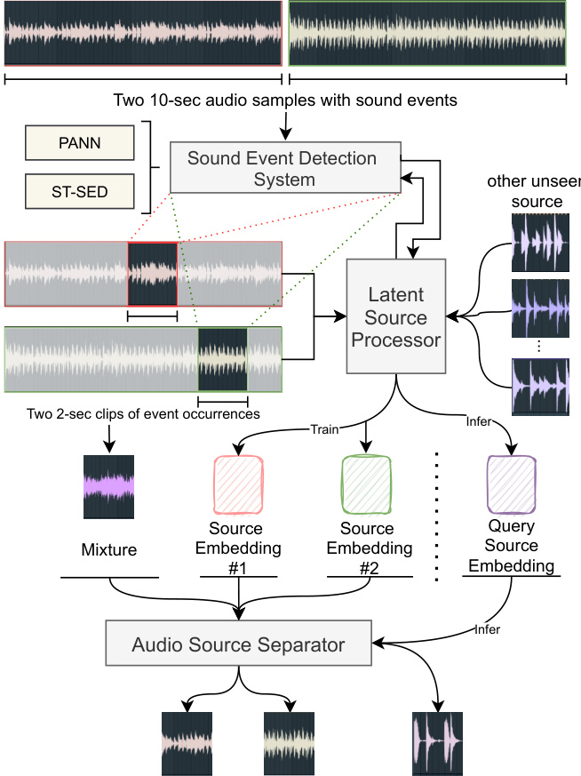
Figure 1: The architecture of our proposed zero-shot separation system.
图 1: 我们提出的零样本 (zero-shot) 分离系统架构。
• We propose a complete pipeline to leverage weaklylabeled audio data in training audio source separation systems. The results show that our utilization of these data is effective. • We design a transformer-based sound event detection system ST-SED. It outperforms the SOTA for sound event detection in AudioSet, while achieving a strong localization performance on the weakly-labeled data. • We employ a single latent source separator for multiple types of audio sources, which saves training time and reduces the number of parameters. Moreover, we experi mentally demonstrate that our approach can support zero-shot generalization to unseen types of sources.
• 我们提出了一套完整的流程,用于在音频源分离系统训练中利用弱标注音频数据。结果表明,我们对这些数据的利用是有效的。
• 我们设计了一个基于Transformer的声音事件检测系统ST-SED。该系统在AudioSet上的声音事件检测性能超越了当前最佳水平(SOTA),同时在弱标注数据上实现了强大的定位性能。
• 我们采用单一潜在源分离器处理多种类型的音频源,这节省了训练时间并减少了参数量。此外,实验证明我们的方法支持对未见源类型的零样本泛化。
Related Work Sound Event Detection and Localization
相关工作 声音事件检测与定位
The sound event detection task is to classify one or more target sound events in a given audio sample. The localization task, or the audio tagging, further requires the model to output the specific time-range of events on the audio timeline. Currently, the convolutional neural network (CNN) (LeCun et al. 1999) is being widely used to detect sound events. The Pretrained Audio Neural Networks (PANN) (Kong et al. 2020a) and the PSLA (Gong, Chung, and Glass 2021b) achieve the current CNN-based SOTA for the sound event detection, with their output feature maps serving as an empirical probability map of events within the audio timeline. For the transformer-based structure, the latest audio spectrogram transformer (AST) (Gong, Chung, and Glass 2021a) re-purposes the visual transformer structure ViT (Dosovitskiy et al. 2021) and DeiT (Touvron et al. 2021) to use the transformer’s class-token to predict the sound event. It achieves the best performance on the sound event detection task in AudioSet. However, it cannot directly localize the events because it outputs only a class-token instead of a featuremap. In this paper, we propose a transformer-based model ST-SED to detect and localize the sound event. Moreover, we use the ST-SED to process the weakly-labeled data that is sent downstream into the following separator.
声音事件检测任务是对给定音频样本中的一个或多个目标声音事件进行分类。定位任务(或称音频标注)则进一步要求模型输出音频时间线上事件的具体时间范围。目前,卷积神经网络 (CNN) (LeCun et al. 1999) 被广泛用于检测声音事件。预训练音频神经网络 (PANN) (Kong et al. 2020a) 和 PSLA (Gong, Chung, and Glass 2021b) 实现了当前基于 CNN 的声音事件检测 SOTA (state-of-the-art) ,其输出特征图作为音频时间线上事件的经验概率图。对于基于 Transformer 的结构,最新的音频频谱图 Transformer (AST) (Gong, Chung, and Glass 2021a) 重新利用了视觉 Transformer 结构 ViT (Dosovitskiy et al. 2021) 和 DeiT (Touvron et al. 2021) ,使用 Transformer 的类别 Token 来预测声音事件。它在 AudioSet 的声音事件检测任务中取得了最佳性能。然而,由于它仅输出类别 Token 而非特征图,因此无法直接定位事件。本文提出了一种基于 Transformer 的模型 ST-SED 来检测和定位声音事件。此外,我们使用 ST-SED 处理弱标注数据,并将其发送到下游的分离器中。
Universal Source Separation
通用源分离
Universal source separation attempts to employ a single model to separate different types of sources. Currently, the query-based model AQMSP (Lee, Choi, and Lee 2019) and the meta-learning model MetaTasNet (Samuel, Ganeshan, and Naradowsky 2020) can separate up to four sources in MUSDB18 dataset in the music source separation task. SuDoRM-RF (Tzinis, Wang, and Smaragdis 2020), the UniConvTasNet (Kavalerov et al. 2019), the PANN-based separator (Kong et al. 2020b), and MSI-DIS (Lin et al. 2021) extend the universal source separation to speech separation, environmental source separation, speech enhancement and music separation and synthesis tasks. However, most existing models require a separation dataset with clean sources and mixtures to train, and only support a limited number of sources that are seen in the training set. An ideal universal source separator should separate as many sources as possible even if they are unseen or not clearly defined in the training. In this paper, based on the architecture from (Kong et al. 2020b), we move further in this direction by proposing a pipeline that can use audio event samples for training a separator that generalizes to diverse and unseen sources.
通用音源分离旨在通过单一模型分离不同类型的音源。目前,基于查询的模型AQMSP (Lee, Choi, and Lee 2019) 和元学习模型MetaTasNet (Samuel, Ganeshan, and Naradowsky 2020) 在音乐音源分离任务中可分离MUSDB18数据集中的最多四种音源。SuDoRM-RF (Tzinis, Wang, and Smaragdis 2020)、UniConvTasNet (Kavalerov et al. 2019)、基于PANN的分离器 (Kong et al. 2020b) 以及MSI-DIS (Lin et al. 2021) 将通用音源分离扩展至语音分离、环境音源分离、语音增强以及音乐分离与合成任务。然而,现有模型大多需要包含纯净音源与混合样本的训练数据集,且仅支持训练集中已见的有限音源类型。理想的通用音源分离器应能分离尽可能多的音源,即使这些音源在训练中未出现或未明确定义。本文基于 (Kong et al. 2020b) 的架构,提出一种利用音频事件样本训练分离器的流程,该分离器可泛化至多样且未见过的音源,从而推动该方向的进一步发展。
Methodology and Pipeline
方法论与流程
In this section, we introduce three components of our source separation model. The sound event detection system is established to refine the weakly-labeled data before it is used by the separation model for training. A query-based source separator is designed to separate audio into different sources. Then an embedding processor is proposed to connect the above two components and allows our model to perform separation on unseen types of audio sources.
在本节中,我们将介绍音源分离模型的三个组成部分。首先建立声音事件检测系统,用于在弱标注数据被分离模型用于训练前对其进行优化。随后设计了一个基于查询的音源分离器,用于将音频分离为不同音源。最后提出一个嵌入处理器来连接上述两个组件,使我们的模型能够对未见过的音频源类型进行分离。
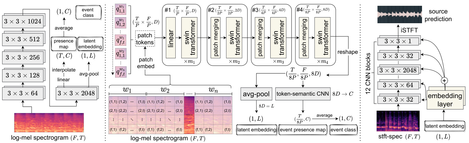
Figure 2: The network architecture of SED systems and the source separator. Left: PANN (Kong et al. 2020a); Middle: our proposed ST-SED; Right: the U-Net-based source separator. All CNNs are named as [2D-kernel size $\times$ channel size].
图 2: SED系统与音源分离器的网络架构。左: PANN (Kong et al. 2020a); 中: 我们提出的ST-SED; 右: 基于U-Net的音源分离器。所有CNN均命名为[2D-核尺寸 $\times$ 通道数]。
Sound Event Detection System
声音事件检测系统
In Audioset, each datum is a 10-sec audio sample with multiple sound events. The only accessible label is what sound events this sample contains (i.e., a multi-hot vector). However, we cannot get accurate start and end times for each sound event in a sample. This raises the problem of extracting a clip from a sample where one sound event most likely occurs (e.g., a 2-sec audio clip). As shown in the upper part of Figure 1, a pipeline is depicted by using a sound event detection (SED) system to process the weakly-labeled data. This system is designed to localize a 2-sec audio clip from a 10-sec sample, which will serve as an accurate sound event occurrence.
在Audioset数据集中,每个数据点都是包含多个声音事件的10秒音频样本。唯一可获取的标签是样本包含哪些声音事件(即一个多热向量)。但我们无法获知样本中每个声音事件精确的起止时间。这引出了如何从样本中提取最可能包含单一声音事件的音频片段(例如2秒片段)的问题。如图1上半部分所示,我们通过声音事件检测(SED)系统处理弱标注数据的流程:该系统被设计用于从10秒样本中定位出2秒音频片段,作为精确的声音事件发生区间。
In this section, we will first briefly introduce an existing SOTA system: Pretrained Audio Neural Networks (PANN) (Left), which serves as the main model to compare in both sound event detection and localization experiments. Then we introduce our proposed system ST-SED (Middle) that leads to better performance than PANN.
在本节中,我们将首先简要介绍现有的SOTA系统:预训练音频神经网络 (Pretrained Audio Neural Networks, PANN) (左),它作为声音事件检测和定位实验中的主要对比模型。然后介绍我们提出的ST-SED系统 (中),其性能优于PANN。
Pretrained Audio Neural Networks As shown in the left of Figure 2, PANN contains VGG-like CNNs (Simonyan and Zisserman 2015) to convert an audio mel-spec tr ogram into a $(T,C)$ featuremap, where $T$ is the number of time frames and $C$ is the number of sound event classes. The model averages the featuremap over the time axis to obtain a final probability vector $(1,C)$ and computes the binary cross-entropy loss between it and the groudtruth label. Since CNNs can capture the information in each time window, the featuremap $(T,C)$ is empircally regarded as a presence probability map of each sound event at each time frame. When determining the latent source embedding for the following pipeline, the penultimate layer’s output $(T,L)$ can be used to obtain its averaged vector $(1,L)$ as the latent source embedding.
预训练音频神经网络
如图 2 左侧所示,PANN 采用类 VGG CNN (Simonyan and Zisserman 2015) 将梅尔频谱图转换为 $(T,C)$ 特征图,其中 $T$ 为时间帧数,$C$ 为声音事件类别数。该模型通过对时间轴取平均得到最终概率向量 $(1,C)$ ,并计算其与真实标签的二元交叉熵损失。由于 CNN 能捕捉每个时间窗口的信息,特征图 $(T,C)$ 可视为各时间帧上各声音事件的存在概率图。在确定后续流程的潜在源嵌入时,可使用倒数第二层输出 $(T,L)$ 的平均向量 $(1,L)$ 作为潜在源嵌入。
Swin Token-Semantic Transformer for SED The transformer structure (Vaswani et al. 2017) and the tokensemantic module (Gao et al. 2021) have been widely used in the image classification and segmentation task and achieve better performance. In this paper, we expect to bring similar improvements to the sound event detection and audio tagging task, which then will contribute also to the separation task. As mentioned in the related work, the audio spectrogram transformer (AST) cannot be applied to audio tagging. Therefore, we refer to swin-transformer (Liu et al. 2021) in order to propose a swin token-semantic transformer for sound event detection (ST-SED). In the middle of Figure 2, a mel-spec tr ogram is cut into different patch tokens with a patch-embed CNN and sent into the transformer in order. We make the time and frequency lengths of the patch equal as $P\times P$ . Further, to better capture the relationship between frequency bins of the same time frame, we first split the mel-spec tr ogram into windows $w_{1},w_{2},...,w_{n}$ and then split the patches in each window. The order of tokens $Q$ follows time $\rightarrow$ frequency $\rightarrow$ window as:
Swin Token-Semantic Transformer 用于声音事件检测
Transformer 结构 (Vaswani et al. 2017) 和 token-semantic 模块 (Gao et al. 2021) 在图像分类和分割任务中已被广泛应用,并取得了优异性能。本文希望将类似改进引入声音事件检测和音频标注任务,从而进一步助力音频分离任务。如相关工作所述,音频频谱 Transformer (AST) 无法直接应用于音频标注任务。因此,我们参考 swin-transformer (Liu et al. 2021) ,提出用于声音事件检测的 swin token-semantic transformer (ST-SED)。
在图 2 中部,梅尔频谱图通过 patch-embed CNN 被切割为多个 patch token 并按序输入 Transformer。我们将 patch 的时频维度统一设为 $P\times P$。此外,为更好捕捉同一时间帧内频点间的关系,我们先将梅尔频谱图分割为窗口 $w_{1},w_{2},...,w_{n}$,再对各窗口进行 patch 划分。token 序列 $Q$ 遵循 时间 $\rightarrow$ 频率 $\rightarrow$ 窗口 的排序规则:

Where $\begin{array}{r}{t=\frac{T}{P},f=\frac{F}{P}}\end{array}$ , $n$ is the number of time windows, and $q_{i,j}^{w_{k}}$ denotes the patch in the position shown by Figure 2. The patch tokens pass through several network groups, each of which contains several transformer-encoder blocks. Between every two groups, we apply a patch-merge layer to reduce the number of tokens to construct a hierarchical representation. Each transformer-encoder block is a swintransformer block with the shifted window attention module (Liu et al. 2021), a modified self-attention module to improve the training efficiency. As illustrated in Figure 2, the shape of the patch tokens is reduced by 8 times from $\begin{array}{r}{\left(\frac{T}{P}\times\frac{\dot{F}}{P},D\right)}\end{array}$ to $(\frac{\stackrel{\cdot}{T}}{8P}\times\frac{F}{8P},8D)$ after 4 network groups.
其中 $\begin{array}{r}{t=\frac{T}{P},f=\frac{F}{P}}\end{array}$ ,$n$ 为时间窗口数量,$q_{i,j}^{w_{k}}$ 表示图 2 所示位置的图像块 (patch) 。这些图像块 token 会通过多个网络组,每组包含若干 transformer-encoder 模块。在每两组之间,我们采用 patch-merge 层来减少 token 数量以构建层次化表征。每个 transformer-encoder 模块都是采用移位窗口注意力机制 (shifted window attention module) [20] 的 swintransformer 模块,这是一种改进的自注意力模块以提升训练效率。如图 2 所示,经过 4 个网络组后,图像块 token 的维度从 $\begin{array}{r}{\left(\frac{T}{P}\times\frac{\dot{F}}{P},D\right)}\end{array}$ 缩减至 $(\frac{\stackrel{\cdot}{T}}{8P}\times\frac{F}{8P},8D)$ ,缩小了 8 倍。
We reshape the final block’s output to $(\frac{T}{8P},\frac{F}{8P},8D)$ Then, we apply a token-semantic 2D-CNN (Gao et al. 2021) with kernel size $(3,{\frac{F}{8P}})$ and padding size $(1,0)$ to integrate all frequency bins, meanwhile map the channel size $8D$ into the sound event classes $C$ . The output $\textstyle({\frac{T}{8P}},C)$ is regarded as a featuremap within time frames in a certain resolution. Finally, we average the featuremap as the final vector $(1,C)$ and compute the binary cross-entropy loss with the ground truth label. Different from traditional visual transformers and AST, our proposed ST-SED does not use the class-token but the averaged final vector from the tokensemantic layer to indicate the sound event. This makes the localization of sound events available in the output. In the practical scenario, we could use the featuremap $\textstyle{\Bigl(}{\frac{T}{8P}},C{\Bigr)}$ to localize sound events. And if we set $8D=L$ , the averaged vector $(1,L)$ of the featuremap $\bigl(\frac{T}{8P},\underline{{{L}}}\bigr)$ can be used as the latent source embedding in line with PANN.
我们将最终块的输出重塑为 $(\frac{T}{8P},\frac{F}{8P},8D)$ ,随后应用一个核大小为 $(3,{\frac{F}{8P}})$ 、填充大小为 $(1,0)$ 的 token-semantic 2D-CNN (Gao et al. 2021) 来整合所有频段,同时将通道数 $8D$ 映射到声音事件类别数 $C$ 。输出 $\textstyle({\frac{T}{8P}},C)$ 被视为特定时间分辨率下的特征图。最后,我们将特征图平均为最终向量 $(1,C)$ ,并与真实标签计算二元交叉熵损失。与传统视觉 Transformer 和 AST 不同,我们提出的 ST-SED 不使用类别 token,而是采用 token-semantic 层的平均输出向量来表征声音事件,这使得声音事件的定位可在输出中实现。实际应用中,我们可以利用特征图 $\textstyle{\Bigl(}{\frac{T}{8P}},C{\Bigr)}$ 进行声音事件定位。若设 $8D=L$ ,则特征图 $\bigl(\frac{T}{8P},\underline{{{L}}}\bigr)$ 的平均向量 $(1,L)$ 可作为符合 PANN 的潜在声源嵌入。
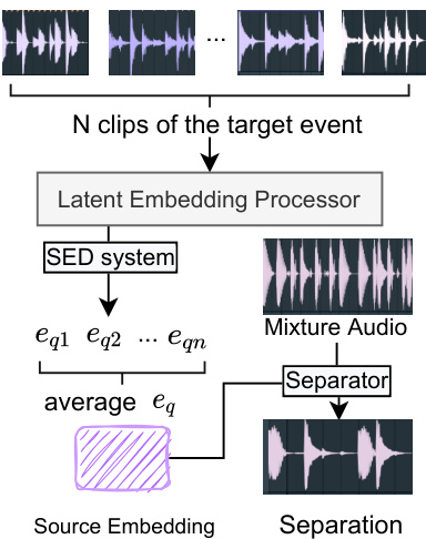
Figure 3: The mechanism to separate an audio into any given source. We collect $N$ clean clips of the target event. Then we take the average of latent source embeddings as the query embedding $e_{q}$ . The separator receives the embedding then performs the separation on the given audio.
图 3: 将音频分离为任意指定声源的机制。我们收集目标事件的 $N$ 段纯净片段,然后计算潜在声源嵌入的平均值作为查询嵌入 $e_{q}$。分离器接收该嵌入后对给定音频执行分离操作。
Query-based Source Separator
基于查询的源分离器
By SED systems, we can localize the most possible occurrence of a given sound event in an audio sample. Then, as shown in the Figure 1, suppose that we want to localize the sound event $s_{1}$ in the sample $x_{1}$ and another event $s_{2}$ in $x_{2}$ , we feed $x_{1},x_{2}$ into the SED system to obtain two featuremaps $m_{1},m_{2}$ . From $m_{1},m_{2}$ we can find the time frame $t_{1},t_{2}$ of the maximum probability on $s_{1}$ , $s_{2}$ , respectively. Finally, we could get two 2-sec clips $c_{1},c_{2}$ as the most possible occurrences of $s_{1},s_{2}$ by assigning $t_{1},t_{2}$ as center frames on two clips, respectively.
通过SED系统,我们可以在音频样本中定位给定声音事件最可能发生的位置。如图1所示,假设我们需要在样本$x_{1}$中定位声音事件$s_{1}$,在$x_{2}$中定位另一个事件$s_{2}$,我们将$x_{1},x_{2}$输入SED系统以获得两个特征图$m_{1},m_{2}$。从$m_{1},m_{2}$中可分别找到$s_{1}$、$s_{2}$最大概率对应的时间帧$t_{1},t_{2}$。最终,通过将$t_{1},t_{2}$分别设为两个片段的中心帧,可得到两个2秒片段$c_{1},c_{2}$作为$s_{1},s_{2}$最可能出现的区间。
Subsequently, we resend two clips $c_{1},c_{2}$ into the SED system to obtain two source embeddings $e_{1},e_{2}$ . Each latent source embedding $(1,L)$ is incorporated into the source separation model to specify which source needs to be separated. The incorporation mechanism will be introduced in detail in the following paragraphs.
随后,我们将两个音频片段 $c_{1},c_{2}$ 重新输入SED系统,得到两个源嵌入向量 $e_{1},e_{2}$。每个潜在源嵌入 $(1,L)$ 会被整合到源分离模型中,以指定需要分离的声源。具体的整合机制将在后续段落中详细介绍。
After we collect $c_{1},c_{2},e_{1},e_{2}$ , we mix two clips as $c=$ $c_{1}+c_{2}$ with energy normalization. Then we send two training triplets $(c,c_{1},e_{1}),(c,c_{2},e_{2})$ into the separator $f$ , respec- tively. We let the separator to learn the following regression:
在收集到 $c_{1},c_{2},e_{1},e_{2}$ 后,我们将两段音频混合为 $c=c_{1}+c_{2}$ 并进行能量归一化。随后将两个训练三元组 $(c,c_{1},e_{1}),(c,c_{2},e_{2})$ 分别送入分离器 $f$ ,使分离器学习以下回归关系:

As shown in the right of Figure 2, we base on U-Net (Ronneberger, Fischer, and Brox 2015) to construct our source separator, which contains a stack of down sampling and upsampling CNNs. The mixture clip $c$ is converted into the spec tr ogram by Short-time Fourier Transform (STFT). In each CNN block, the latent source embedding $e_{j}$ is incorporated by two embedding layers producing two featuremaps and added into the audio feature maps before passing through the next block. Therefore, the network will learn the relationship between the source embedding and the mixture, and adjust its weights to adapt to the separation of different sources. The output spec tr ogram of the fi- nal CNN block is converted into the separate waveform $c\prime$ by inverse STFT (iSTFT). Suppose that we have $n$ training triplets ${(c^{1},c_{j}^{1},e_{j}^{1}),(c^{2},c_{j}^{2},e_{j}^{\hat{2}}},...,(c^{n},c_{j}^{n},e_{j}^{n})}$ , we apply the Mean Absolute Error (MAE) to compute the loss between separate waveforms $C^{\prime}={c^{1\prime},c^{2\prime},...,c^{n\prime}}$ and the target source clips $C_{j}={c_{j}^{1},c_{j}^{2},...,\dot{c}_{j}^{n}}$ :
如图 2 右侧所示,我们基于 U-Net (Ronneberger, Fischer, and Brox 2015) 构建源分离器,该结构包含堆叠的下采样和上采样 CNN。混合音频片段 $c$ 通过短时傅里叶变换 (STFT) 转换为频谱图。在每个 CNN 模块中,潜在源嵌入 $e_{j}$ 通过两个嵌入层生成两个特征图,并添加到音频特征图中再传入下一模块。因此,网络将学习源嵌入与混合音频之间的关系,并调整权重以适应不同源的分离。最终 CNN 模块输出的频谱图通过逆 STFT (iSTFT) 转换为分离波形 $c\prime$。假设我们有 $n$ 个训练三元组 ${(c^{1},c_{j}^{1},e_{j}^{1}),(c^{2},c_{j}^{2},e_{j}^{\hat{2}}},...,(c^{n},c_{j}^{n},e_{j}^{n})}$,采用平均绝对误差 (MAE) 计算分离波形 $C^{\prime}={c^{1\prime},c^{2\prime},...,c^{n\prime}}$ 与目标源片段 $C_{j}={c_{j}^{1},c_{j}^{2},...,\dot{c}_{j}^{n}}$ 之间的损失:

Combining these two components together, we could utilize more datasets (i.e. containing sufficient audio samples but without separation data) in the source separation task. Indeed, it also indicates that we no longer require clean sources and mixtures for the source separation task (Kong et al. 2020b, 2021) if we succeed in using these datasets to achieve a good performance.
将这两个组件结合起来,我们可以在音源分离任务中利用更多数据集(即包含充足音频样本但缺乏分离数据的数据集)。事实上,这也意味着如果我们能成功利用这些数据集实现良好性能,就不再需要为音源分离任务准备干净的源信号和混合信号 (Kong et al. 2020b, 2021)。
Zero-shot Learning via Latent Source Embeddings
零样本学习通过潜在源嵌入实现
The third component, the embedding processor, serves as a communicator between the SED system and the source separator. As shown in Figure 1, during the training, the function of the latent source embedding processor is to obtain the latent source embedding $e$ of given clips $c$ from the SED system, and send the embedding into the separator. And in the inference stage, we enable the processor to utilize this model to separate more sources that are unseen or undefined in the training set.
第三个组件是嵌入处理器 (embedding processor),它充当SED系统和源分离器之间的通信桥梁。如图1所示,在训练过程中,潜在源嵌入处理器的功能是从SED系统中获取给定片段$c$的潜在源嵌入$e$,并将该嵌入发送到分离器。在推理阶段,我们使处理器能够利用该模型分离训练集中未见或未定义的更多声源。
Formally, suppose that we need to separate an audio $x_{q}$ according to a query source $s_{q}$ . In order to get the latent source embedding $e_{q}$ , we first need to collect $N$ clean clips of this source ${\dot{c_{q1}},c_{q2},...,c_{q N}}$ . Then we feed them into the SED system to obtain the latent embeddings ${e_{q1},e_{q2},...,e_{q N}}$ . The $e_{q}$ is obtained by taking the average of them:
形式上,假设我们需要根据查询源 $s_{q}$ 分离音频 $x_{q}$。为了获取潜在源嵌入 $e_{q}$,首先需要收集该源的 $N$ 个干净片段 ${\dot{c_{q1}},c_{q2},...,c_{q N}}$,然后将其输入SED系统以获得潜在嵌入 ${e_{q1},e_{q2},...,e_{q N}}$。最终通过取平均值得到 $e_{q}$:

Then, we use $e_{q}$ as the query for the source $s_{q}$ and separate $x_{q}$ into the target track $f(x_{q},e_{q})$ . A visualization of this process is depicted in Figure 3.
然后,我们使用 $e_{q}$ 作为源 $s_{q}$ 的查询,并将 $x_{q}$ 分离为目标轨道 $f(x_{q},e_{q})$ 。该过程的可视化如图 3 所示。
The 527 classes of Audioset are ranged from ambient natural sounds to human activity sounds. Most of them are not clean sources as they contain other backgrounds and event sounds. After training our model in Audioset, we find that the model is able to achieve a good performance on separating unseen sources. According to (Wang et al. 2019), we declare that this follows a Class-Trans duct ive InstanceInductive (CTII) setting of zero-shot learning (Wang et al. 2019) as we train the separation model by certain types of sources and use unseen queries to let the model separate unseen sources.
AudioSet的527个类别涵盖了从自然环境声到人类活动声的广泛范围。大多数声源并非纯净样本,往往包含背景音和其他事件声音。通过在AudioSet上训练模型,我们发现该模型能够有效分离未见过的声源类型。根据 (Wang et al. 2019) 的研究,我们将其归类为类传导实例归纳 (CTII) 的零样本学习设定:模型通过特定类型声源进行训练后,能够根据未见过的查询指令分离新声源类型 (Wang et al. 2019)。
Table 1: The mAP results in Audioset evaluation set.
表 1: Audioset评估集的mAP结果
| Model | mAP |
|---|---|
| AudioSetBaseline (2017) | 0.314 |
| DeepRes. (2019) | 0.392 |
| PANN. (2020a) | 0.434 |
| PSLA. (2021b) | 0.443 |
| AST. (single) w/o. pretrain (2021a) | 0.368 |
| AST. (single) (2021a) | 0.459 |
| 768-dST-SED | 0.467 |
| 768-d ST-SEDw/o.pretrain | 0.458 |
| 2048-d ST-SED w/o.pretrain | 0.459 |
Experiment
实验
There are two experimental stages for us to train a zero-shot audio source separator. First, we need to train a SED system as the first component. Then, we train an audio source separator as the second component based on the processed data from the SED system. In the following subsections, we will introduce the experiments in these two stages.
我们训练零样本音频源分离器的实验分为两个阶段。首先,需要训练一个声音事件检测(SED)系统作为第一组件。然后,基于SED系统处理后的数据,训练音频源分离器作为第二组件。以下小节将介绍这两个阶段的实验。
Sound Event Detection
声音事件检测
Dataset and Training Details We choose AudioSet to train our sound event detection system ST-SED. It is a largescale collection of over 2 million 10-sec audio samples and labeled with sound events from a set of 527 labels. Following the same training pipeline with (Gong, Chung, and Glass 2021a), we use AudioSet’s full-train set (2M samples) for training the ST-SED model and its evaluation set (22K samples) for evaluation. To further evaluate the localization performance, we use DESED test set (Serizel et al. 2020), which contains 692 10-sec audio samples with strong labels (time boundaries) of 2765 events in total. All labels in DESED are the subset (10 classes) of AudioSet’s sound event classes. In that, we can directly map AudioSet’s classes into DESED’s classes. There is no overlap between AudioSet’s full-train set and DESED test set. And there is no need to use DESED training set because AudioSet’s fulltrain set contains more training data.
数据集与训练细节
我们选择AudioSet来训练声音事件检测系统ST-SED。该数据集包含超过200万段10秒音频样本,并使用527种标签标注声音事件。遵循(Gong, Chung, and Glass 2021a)相同的训练流程,我们使用AudioSet的全训练集(200万样本)训练ST-SED模型,并用其评估集(2.2万样本)进行评估。
为进一步评估定位性能,我们采用DESED测试集(Serizel et al. 2020),该数据集包含692段10秒音频样本,带有2765个事件的强标注(时间边界)。DESED所有标签均为AudioSet声音事件类别的子集(10类),因此可直接将AudioSet类别映射到DESED类别。
AudioSet全训练集与DESED测试集无重叠,且无需使用DESED训练集,因为AudioSet全训练集已包含更丰富的训练数据。
For the pre-processing of audio, all samples are converted to mono as 1 channel by $32\mathrm{kHz}$ sampling rate. To compute STFTs and mel-spec tro grams, we use 1024 window size and 320 hop size. As a result, each frame is $\frac{320}{32000}=0.01$ sec. The number of mel-frequency bins is $F=64$ . Each 10-sec sample constructs 1000 time frames and we pad them with 24 zero-frames $T=1024)$ . The shape of the output featuremap is (1024, 527) ( $C=527$ ). The patch size is $4\times4$ and the time window is 256 frames in length. We propose two settings for the ST-SED with a latent dimension size $L$ of 768 or 2048. We adopt the 768-d model to make use of the swin-transformer ImageNet-pretrained model for achieving a potential best result. And we adopt the 2048-d model in the following separation experiment because it shares the consistent latent dimension size with PANN’s. We set 4 network groups in the ST-SED, containing 2,2,6, and 2 swintransformer blocks respectively.
在音频预处理阶段,所有样本均转换为单声道(1通道),采样率为$32\mathrm{kHz}$。计算短时傅里叶变换(STFT)和梅尔频谱时,我们采用1024的窗口大小和320的跳跃步长,因此每帧时长为$\frac{320}{32000}=0.01$秒。梅尔频段数设为$F=64$,每个10秒样本生成1000个时间帧,并补零24帧$T=1024)$。输出特征图的维度为(1024, 527)( $C=527$ )。设置$4\times4$的块大小和256帧长度的时间窗口。针对ST-SED模型,我们提出两种潜在维度尺寸$L$的配置方案:768或2048。采用768维模型是为了利用Swin-Transformer在ImageNet上的预训练模型以获取最佳性能,而分离实验中选择2048维模型因其与PANN模型的潜在维度保持一致。ST-SED网络设置4个组结构,分别包含2、2、6、2个Swin-Transformer模块。
| 验证集: AudioSet评估集 | |||
|---|---|---|---|
| 指标-SDR: dB | 混合 | 纯净 | 静音 |
| 527-dPANN-SEP(2020b) | 7.38 | 8.89 | 11.00 |
| 2048-dPANN-SEP | 9.42 | 13.96 | 15.89 |
| 2048-dST-SED-SEP | 10.55 | 27.83 | 16.64 |
Table 2: The SDR performance of different models with different source embeddings in the validation set.
表 2: 验证集中不同模型使用不同源嵌入(source embeddings)的SDR性能对比。
We implement the ST-SED in PyTorch2, train it with a batch size of 128 and the AdamW optimizer ( $\beta_{1}\mathrm{=}0.9$ , $\beta_{2}{=}0.999$ , $\mathrm{eps}{=}1\mathrm{e}{-}8$ , decay $=0.05\$ ) (Kingma and Ba 2015) in 8 NVIDIA Tesla V-100 GPUs in parallel. We adopt a warmup schedule by setting the learning rate as 0.05, 0.1, 0.2 in the first three epochs, then the learning rate is halved every ten epochs until it returns to 0.05.
我们在PyTorch2中实现了ST-SED,使用128的批量大小和AdamW优化器 ( $\beta_{1}\mathrm{=}0.9$ , $\beta_{2}{=}0.999$ , $\mathrm{eps}{=}1\mathrm{e}{-}8$ , decay $=0.05\$ ) (Kingma and Ba 2015),在8块NVIDIA Tesla V-100 GPU上并行训练。采用学习率预热策略:前三个周期分别设为0.05、0.1、0.2,之后每十个周期学习率减半直至回落到0.05。
AudioSet Results Following the standard evaluation pipeline, we use the mean average precision (mAP) to verify the classification performance on Audioset’s evaluation set. In Table 1, we compare the ST-SED with previous SOTAs including the latest PANN, PSLA, and AST. Among all models, PSLA, AST, and our 768-d ST-SED apply the ImageNet-pretrained models. Specifically, PSLA uses the pretrained Efficient Net (Tan and Le 2019); AST uses the pretrained DeiT; and 768-d ST-SED uses the pretrained swin-transformer in Swin-T/C24 setting3. We also provide the mAP result of the 768-d ST-SED without pre training for comparison. For the 2048-d ST-SED, we train it from zero because there is no pretrained model. For the AST, we compare our model with its single model’s report instead of the ensemble one to ensure the fairness of the experiment. All ST-SEDs are converged around 30-40 epochs in about 20 hours’ training.
AudioSet 实验结果
按照标准评估流程,我们采用平均精度均值 (mAP) 验证模型在 Audioset 评估集上的分类性能。表 1 将 ST-SED 与此前的 SOTA 方法(包括最新的 PANN、PSLA 和 AST)进行对比。所有模型中,PSLA、AST 以及我们的 768 维 ST-SED 均采用 ImageNet 预训练模型:具体而言,PSLA 使用预训练的 Efficient Net (Tan and Le 2019);AST 使用预训练的 DeiT;而 768 维 ST-SED 采用 Swin-T/C24 配置下的预训练 swin-transformer。我们还提供了未经过预训练的 768 维 ST-SED 的 mAP 结果作为对比。对于 2048 维 ST-SED,由于缺乏预训练模型,我们从头开始训练。为确保实验公平性,与 AST 对比时我们采用其单模型报告结果而非集成模型。所有 ST-SED 模型均在约 20 小时训练后于 30-40 个 epoch 达到收敛。
From Table 1, we find that the 768-d pretrained ST-SED achieves a new mAP SOTA as 0.467 in Audioset. Moreover, our 768-d and 2048-d ST-SEDs without pre training can also achieve the pre-SOTA mAP as 0.458 and 0.459, while the AST without pre training could only achieve a low mAP as 0.368. This indicates that the ST-SED is not limited to the pre training parameters of the computer vision model, and can be used more flexibly in audio tasks.
从表1中我们发现,768维预训练的ST-SED在Audioset上实现了0.467的mAP新SOTA。此外,我们未经预训练的768维和2048维ST-SED也能分别达到0.458和0.459的预SOTA级mAP,而未经预训练的AST仅能达到0.368的低mAP。这表明ST-SED不受限于计算机视觉模型的预训练参数,能更灵活地应用于音频任务。
DESED Results We conduct an experiment on DESED test set to evaluate the localization performance of PANN and the 2048-d ST-SED. We do not include AST and PSLA since AST does not directly support the event localization and the PSLA’s code is not published. We use the eventbased F1-score on each class as the evaluation metric, implemented by a Python library psds eval4.
DESED实验结果
我们在DESED测试集上进行实验,评估PANN和2048维ST-SED的定位性能。由于AST不直接支持事件定位且PSLA代码未公开,未纳入AST和PSLA模型。采用基于事件的每类F1分数作为评估指标,通过Python库psds_eval实现。
The F1-scores on all 10 classes in DESED by two models are shown in Table 3. We find that the 2048-d ST-SED achieves better F1-scores on 8 classes and a better average F1-score than PANN. A large increment is on the Frying class as increasing the F1-score by 40.92. However, we also notice that the F1-scores on Speech class and Cleaner class are dropped when using ST-SED, indicating that there are still some improvements for a better localization performance.
表3展示了两种模型在DESED数据集上10个类别的F1分数。我们发现,2048维ST-SED模型在8个类别上取得了优于PANN的F1分数,平均F1分数也更高。其中Frying类别的提升幅度最大,F1分数增加了40.92。但我们也注意到,ST-SED模型在Speech和Cleaner类别上的F1分数有所下降,这表明其在定位性能方面仍有改进空间。
Table 3: The F1-score results on each class of two models in DESED test set.
表 3: DESED测试集上两个模型在各类别的F1分数结果。
| Model | Alarm | Blender | Cat | Dishes | Dog | Shaver | Frying | Water | Speech | Cleaner | Average |
|---|---|---|---|---|---|---|---|---|---|---|---|
| PANN | 34.33 | 42.35 | 36.31 | 17.60 | 35.82 | 23.81 | 9.30 | 30.58 | 69.68 | 51.01 | 35.08 |
| ST-SED | 44.66 | 52.23 | 69.98 | 27.35 | 49.93 | 43.90 | 50.22 | 42.76 | 45.11 | 41.55 | 46.77 |
From the above experiments, we can conclude that the ST-SED achieves the best sound event detection results and the superior results on localization performance in AudioSet and DESED. These results are sufficient for us to use the 2048-d ST-SED model to conduct the following separation experiments. It is better to evaluate the ST-SED on datasets. Due to the page limit, we leave these as future work.
从上述实验中,我们可以得出结论:ST-SED在AudioSet和DESED数据集上实现了最佳的声音事件检测效果,并在定位性能上取得优越表现。这些结果足以支持我们采用2048维ST-SED模型进行后续分离实验。在数据集上评估ST-SED效果更佳,但由于篇幅限制,这部分工作将留待未来完成。
Audio Source Separation
音频源分离
Dataset and Training Details We train our audio separator in AudioSet full-train set, validate it in Audioset evaluation set, and evaluate it in MUSDB18 test set as following the 6th community-based Signal Separation Evaluation Campaign (SiSEC 2018). MUSDB18 contains 150 songs with a total duration of 3.5 hours in different genres. Each song provides a mixture track and four original stems: vocal, drum, bass, and other. All SOTAs are trained with MUSDB18 training set (100 songs) and evaluated in its test set (50 songs). Different from these SOTAs, we train our model only with Audioset full-train set other than MUSDB and directly evaluate it in MUSDB18 test set.
数据集与训练细节
我们使用AudioSet全训练集训练音频分离器,在AudioSet评估集进行验证,并按照第六届社区信号分离评估竞赛(SiSEC 2018)的标准在MUSDB18测试集上评估。MUSDB18包含150首不同流派的歌曲,总时长为3.5小时,每首歌曲提供混合音轨及四个原始音轨:人声、鼓、贝斯和其他。所有先进模型(SOTA)均使用MUSDB18训练集(100首歌曲)训练并在其测试集(50首歌曲)评估。与这些SOTA不同,我们仅使用AudioSet全训练集(而非MUSDB)训练模型,并直接在MUSDB18测试集上评估。
Since Audioset is not a natural separation dataset (i.e., no mixture data), to construct the training set and the validation set, during each training step, we sample two classes from 527 classes and randomly take each sample $x_{1},x_{2}$ from two classes in the full-train set. We implement a balanced sampler that all classes will be sampled equally during the whole training. During the validation stage, we follow the same sampling paradigm to construct 5096 audio pairs from Audioset evaluation set and fix these pairs. By setting a fixed random seed, all models will face the same training data and the validation data.
由于Audioset并非自然分离数据集(即不包含混合数据),为构建训练集和验证集,我们在每个训练步骤中从527个类别中采样两个类,并从完整训练集中随机选取各类样本$x_{1},x_{2}}$。我们实现了平衡采样器,确保所有类别在整个训练过程中被均匀采样。验证阶段采用相同采样范式,从Audioset评估集构建5096个固定音频对,并通过设置固定随机种子保证所有模型使用相同的训练数据和验证数据。
For the model design, our SED system has two choices: PANN or ST-SED. And the separator we apply comprises 6 encoder blocks and 6 decoder blocks. In encoder blocks, the numbers of channels are namely 32, 64, 128, 256, 512, 1024. In decoder blocks, they are reversed (i.e., from 1024 to 32). There is a final convolution kernel that converts 32 channels into the output audio channel. Batch normalization (Ioffe and Szegedy 2015) and ReLU non-linearity (Agarap 2018) are used in each block. The final output is a spectrogram, which can be converted into the final separate audio $c\prime$ by iSTFT. Similarly, we implement our separator in PyTorch and train it with the Adam optimizer ( $\beta_{1}{=}0.9$ , $\beta_{2}{=}0.999$ , eps=1e-8, decay $\mathrm{\ddot{=}}0$ ), the learning rate 0.001 and the batch size of 64 in 8 NVIDIA Tesla V-100 GPUs in parallel.
在模型设计方面,我们的SED系统有两种选择:PANN或ST-SED。所使用的分离器包含6个编码器块和6个解码器块。编码器块中的通道数分别为32、64、128、256、512、1024,解码器块则相反(即从1024到32)。最后一个卷积核将32个通道转换为输出音频通道。每个块都使用了批量归一化 (Ioffe and Szegedy 2015) 和ReLU非线性激活 (Agarap 2018)。最终输出是一个频谱图,可通过iSTFT转换为最终的分离音频$c\prime$。同样,我们使用PyTorch实现分离器,并在8块NVIDIA Tesla V-100 GPU上并行训练,采用Adam优化器 ($\beta_{1}{=}0.9$,$\beta_{2}{=}0.999$,eps=1e-8,衰减$\mathrm{\ddot{=}}0$),学习率为0.001,批量大小为64。
| 标准先进模型 | vocal | drum | bass | other |
|---|---|---|---|---|
| WaveNet (2019) | 3.25 | 4.22 | 3.21 | 2.25 |
| WK (2014) | 3.76 | 4.00 | 2.94 | 2.43 |
| RGT1 (2018) | 3.85 | 3.44 | 2.70 | 2.63 |
| Spec-U-Net (2018) | 5.74 | 4.66 | 3.67 | 3.40 |
| UHL2 (2017) | 5.93 | 5.92 | 5.03 | 4.19 |
| MMDenseLSTM (2018) | 6.60 | 6.41 | 5.16 | 4.15 |
| Open Unmix (2019) | 6.32 | 5.73 | 5.23 | 4.02 |
| Demucs (2019) | 6.21 | 6.50 | 6.21 | 3.80 |
| 基于查询的模型 (使用MUSDB18训练) | vocal | drum | bass | other |
|---|---|---|---|---|
| AQMSP-Mean (2019) | 4.90 | 4.34 | 3.09 | 3.16 |
| Meta-TasNet (2020) | 6.40 | 5.91 | 5.58 | 4.19 |
| 零样本模型 (未使用MUSDB18训练) | vocal | drum | bass | other |
|---|---|---|---|---|
| 527-d PANN-SEP | 4.16 | 0.95 | -0.86 | -2.65 |
| 2048-dPANN-SEP | 6.06 | 5.00 | 3.38 | 2.86 |
| 2048-dST-SED-SEP | 6.15 ±.22 | 5.44 ±.32 | 3.80 ±.23 | 3.05 ±.20 |
Table 4: The SDR performance in MUSDB18 test set. All models are categorized into three slots.
表 4: MUSDB18测试集中的SDR性能表现。所有模型分为三个档位。
Evaluation Metrics We use source-to-distortion ratio (SDR) as the metric to evaluate our separator. For the validation set, we compute three SDR metrics between the prediction and the ground truth in different separation targets:
评估指标
我们采用信源失真比(SDR)作为分离器的评估指标。在验证集上,我们针对不同分离目标计算预测结果与真实值之间的三种SDR指标:
• mixture-SDR’s target: $f(c_{1}+c_{2},e_{j})\mapsto c_{j}$ • clean-SDR’s target: $f(c_{j},e_{j})\mapsto c_{j}$ • silence-SDR’s target: $f(c_{\neg j},e_{j})\mapsto\mathbf{0}$
- mixture-SDR 的目标:$f(c_{1}+c_{2},e_{j})\mapsto c_{j}$
- clean-SDR 的目标:$f(c_{j},e_{j})\mapsto c_{j}$
- silence-SDR 的目标:$f(c_{\neg j},e_{j})\mapsto\mathbf{0}$
Where the symbol $\neg j$ denotes any clip which does not share the same class with the $j$ -th clip. In our setting, $\neg1=2$ and $\neg2=1$ . The clean SDR is to verify if the model can maintain the clean source given the self latent source embedding. The silence SDR is to verify if the model can separate nothing if there is no target source in the given audio. These help us understand if the model can be generalized to more general separation scenarios only by using the mixture training. For the testing, we only compute the mixture SDR between each stem and each original song in MUSDB18 test set. Each song is divided into 1-sec clips. The song’s SDR is the median SDR over all clips. And the final SDR is the median SDR over all songs.
其中符号 $\neg j$ 表示与第 $j$ 个片段不属于同一类别的任何片段。在我们的设定中,$\neg1=2$ 且 $\neg2=1$。干净 SDR 用于验证模型在给定自身潜在源嵌入时能否保持干净的源。静音 SDR 用于验证当给定音频中不存在目标源时,模型是否能分离出空内容。这有助于我们理解模型是否仅通过混合训练就能泛化到更一般的分离场景。测试时,我们仅计算 MUSDB18 测试集中每个音轨与每首原曲之间的混合 SDR。每首歌曲被分割为 1 秒的片段,歌曲的 SDR 是所有片段 SDR 的中位数,而最终的 SDR 是所有歌曲 SDR 的中位数。
The Choice of Source Embeddings We choose three source embeddings for our separator: (1) the 527-d presence probability vector from PANN, referring to (Kong et al. 2020b); (2) the 2048-d latent embedding from PANN’s penultimate layer; and (3) the 2048-d latent embedding from ST-SED. This helps to verify if the latent source embedding can perform a better representation for separation, and if the embedding from ST-SED is better than that from PANN.
源嵌入的选择
我们为分离器选择了三种源嵌入:(1) 来自PANN的527维存在概率向量,参考(Kong et al. 2020b);(2) 来自PANN倒数第二层的2048维潜在嵌入;(3) 来自ST-SED的2048维潜在嵌入。这有助于验证潜在源嵌入是否能更好地表示分离任务,以及ST-SED的嵌入是否优于PANN的嵌入。
Table 5: The SDR performance of the 2048-d ST-SED-SEP in the zero-shot verification experiment.
| 类别 | 对话 | 耳语 | 鼓掌 | 猫叫 | 管弦乐 | 飞机 | 中型引擎 | 倒水 | 刮擦 | 吱嘎声 | 平均 |
|---|---|---|---|---|---|---|---|---|---|---|---|
| 混合-SDR | 9.08 | 8.04 | 9.67 | 9.49 | 9.18 | 8.47 | 8.31 | 7.92 | 8.42 | 6.56 | 8.52 |
| 纯净-SDR | 17.44 | 10.50 | 17.78 | 15.01 | 10.06 | 13.09 | 14.85 | 14.28 | 15.52 | 13.79 | 14.23 |
| 静音-SDR | 14.05 | 13.86 | 14.45 | 17.63 | 12.08 | 11.97 | 11.56 | 12.76 | 13.95 | 13.61 | 13.59 |
表 5: 2048维ST-SED-SEP在零样本验证实验中的SDR性能
In the training and validation stage, we get each latent source embedding directly from each 2-sec clip according to the pipeline in Figure 1. After picking the best model in the validation set, we follow Figure 3 to get the query source embeddings in MUSDB18. Specifically, we collect all separate tracks in the highlight version of MUSDB10 training set (30 secs in each song, 100 songs in total) and take the average of their embeddings on each source as four queries: vocal, drum, bass, and other.
在训练和验证阶段,我们根据图1的流程直接从每个2秒片段中获取潜在源嵌入。在验证集中选出最佳模型后,按照图3的方法获取MUSDB18中的查询源嵌入。具体而言,我们收集MUSDB10训练集高光版本(每首歌30秒,共100首)中的所有分离音轨,并计算每个源(人声、鼓、贝斯和其他)嵌入的平均值作为四个查询。
Separation Results Table 2 shows the SDRs of two models in the validation set. We could clearly figure out that when using the 2048-d latent source embedding, PANN achieves better performance in increasing three types of SDR by $2{-}4~\mathrm{dB}$ than that of 527-d model. A potential rea- son is that the extra capacity of the 2048-d embedding space helped the model better capture the feature of the sound comparing to the 527-d probability embedding. In that, the model can receive more disc rim i native embeddings and perform a more accurate separation.
分离结果
表 2 展示了验证集上两种模型的SDR (Source-to-Distortion Ratio) 指标。可以明显看出,当使用2048维潜在源嵌入时,PANN模型在三种SDR指标上均比527维模型提升了 $2{-}4~\mathrm{dB}$。潜在原因是2048维嵌入空间的额外容量帮助模型更好地捕捉声音特征(相比527维概率嵌入)。这使得模型能获得更具判别性的嵌入,从而实现更精准的分离。
Then we pick the best models of 527-d PANN-SEP, 2048- d PANN-SEP, 2048-d ST-SED-SEP and evaluate them in MUSDB18. As shown in Table 4, there are three categories of models: (1) Standard Model: these models can only separate one source, in that they need to train 4 models to separate each source in MUSDB18. (2) Query-based Model: these models can separate four sources in one model. Both models in (1) and (2) require the training data in MUSDB training set and cannot generalize to separate other sources. And (3) Zero-shot Model: our proposed models can separate four sources in one model without any MUSDB18 training data. Additionally, they can even separate more sources. Specifically, for our proposed 2048-d ST-SED model, we repeat the training three times with different random seeds.
然后我们选取527维PANN-SEP、2048维PANN-SEP和2048维ST-SED-SEP的最佳模型,在MUSDB18上进行评估。如表4所示,模型分为三类:(1) 标准模型:这些模型只能分离一个音源,需要训练4个模型来分别分离MUSDB18中的每个音源。(2) 基于查询的模型:这些模型可以在一个模型中分离四个音源。第(1)和(2)类模型都需要MUSDB训练集中的数据进行训练,无法泛化到其他音源分离任务。(3) 零样本模型:我们提出的模型可以在一个模型中分离四个音源,且无需任何MUSDB18训练数据。此外,它们还能分离更多音源。具体来说,对于我们提出的2048维ST-SED模型,我们使用不同的随机种子重复训练了三次。
From Table 4 our proposed model 2048-d ST-SED-SEP outperforms PANN-SEP models in all SDRs (6.15, 5.44, 3.80, 3.05). The SDRs in vocal, drum, and bass are compatible with standard and query-based SOTAs. However, we observe a relatively low SDR in the ”other” source. One possible reason is that we compute a wrong ”other” embedding for separation by averaging over all source embedding of ”other” in MUSDB18 training set. But this ”other” embed- ding might not be a general embedding because “other” denotes different instruments and timbres in different tracks. Another observation lies in the relatively large standard deviations of all four instruments. One possible reason is that the separation quality is related to the random combination of training data, and different orders may cause differences on some specific types of sounds. One further improving idea is to increase the numbers of combinations (e.g., three instead of two). These sub-topics can be further researched in the future.
从表4可以看出,我们提出的2048-d ST-SED-SEP模型在所有SDR指标(6.15、5.44、3.80、3.05)上都优于PANN-SEP模型。其中人声、鼓声和贝斯的SDR表现与标准及基于查询的SOTA方法相当。然而在"其他"音源上观察到相对较低的SDR值,可能原因是我们通过平均MUSDB18训练集中所有"其他"音源的嵌入来计算分离用的错误"其他"嵌入。但这种"其他"嵌入可能不具备普适性,因为不同曲目中"其他"代表着不同乐器和音色。另一个现象是四种乐器的标准差都较大,可能原因是分离质量与训练数据的随机组合顺序相关,不同排序可能导致特定类型声音的分离效果差异。一个改进思路是增加组合数量(例如三组而非两组),这些子课题值得未来进一步研究。
In summary, the most novel and surprising observation is that our proposed audio separator succeeds in separating 4 sources in MUSDB18 test set without any of its training data but only Audioset. The model performs as a zero-shot separator by using any latent source embedding collected from accessible data, to separator any source it faces.
总之,最新颖且令人惊讶的发现是,我们提出的音频分离器在仅使用Audioset数据(未使用任何MUSDB18训练数据)的情况下,成功分离了MUSDB18测试集中的4种音源。该模型通过利用从可获取数据中收集的潜在音源嵌入(latent source embedding),以零样本方式分离任意遇到的音源。
Zero-Shot Verification
零样本验证
In this section, we conduct another experiment to let the model separate sources that are held-out from training. We first select 10 sound event classes in Audioset. Then during the training, we remove all data of these 10 classes. The model only learns how to separate clips mixed by the left 517 classes. During the evaluation, we construct 1000 $(100\times10)$ mixture samples in Audioset evaluation set whose constituents only belong to these 10 classes. Then we calculate the mixture SDR, the clean SDR, and the silence SDR of them.
在本节中,我们进行了另一项实验,让模型分离训练时未接触的声源。首先从Audioset中选取10个声音事件类别,随后在训练阶段移除这10个类别的所有数据。模型仅学习如何分离由剩余517个类别构成的混合音频片段。评估阶段,我们在Audioset评估集中构建了1000个$(100\times10)$混合样本,其成分仅属于这10个类别,随后计算它们的混合SDR、纯净SDR及静默SDR。
Table 5 shows the results by the 2048-d ST-SED model. We can find that the model can still separate the held-out sources well by achieving the average mixture SDR, clean SDR, and silence SDR as 8.52 dB, $14.23:\mathrm{dB}$ , and $13.59\mathrm{dB}$ . The detailed SDR distribution of these 1000 samples is depicted in the open source repository. The intrinsic reason for this good performance is that the SED system captures many features of 517 sound classes in its latent space. And it generalizes to regions of the embedding space it never saw during training, which the unseen 10 classes lie in. Finally, the separator utilizes these features in the embedding to separate the target source. The zero-shot setting of our model is essentially built by a solid feature extraction mechanism and a latent source separator.
表 5 展示了 2048 维 ST-SED 模型的结果。我们发现该模型仍能有效分离未参与训练的声源,平均混合 SDR、纯净 SDR 和静音 SDR 分别达到 8.52 dB、$14.23:\mathrm{dB}$ 和 $13.59\mathrm{dB}$。这 1000 个样本的详细 SDR 分布已发布于开源代码库。其优异性能的内在原因是 SED 系统在潜空间捕获了 517 种声音类别的特征,并能泛化至训练时未见的嵌入空间区域(未参与的 10 个类别即位于该区域)。最终,分离器利用嵌入空间中的这些特征来分离目标声源。本模型的零样本能力本质上由稳健的特征提取机制和潜在声源分离器共同构建。
Conclusion and Future Work
结论与未来工作
In this paper, we propose a zero-shot audio source separator that can utilize weakly-labeled data to train, target different sources to separate, and support more unseen sources. We train our model in Audioset while evaluating it in MUSDB18 test set. The experimental results show that our model outperforms the query-based SOTAs, meanwhile achieves a compatible result with standard supervised models. We further verify our model in a complete zero-shot setting to prove its generalization ability. With our model, more weakly-labeled audio data can be trained for the source separation problem. And more sources can be separated via one model. In future work, since audio embeddings have been widely used in other audio tasks such as music recommendation (Chen et al. 2021) and music generation (2019; 2020; 2021; 2020; 2020), we expect to use these audio embeddings as source queries to see if they can capture different audio features and lead to better separation performance.
本文提出了一种零样本音频源分离方法,该方法可利用弱标注数据进行训练,针对不同目标源进行分离,并支持更多未见过的声源。我们在Audioset上训练模型,并在MUSDB18测试集上评估。实验结果表明,该模型性能优于基于查询的SOTA方法,同时达到了与标准监督模型相当的结果。我们进一步在完全零样本设置下验证模型,证明了其泛化能力。通过该模型,更多弱标注音频数据可用于解决源分离问题,且单一模型可分离更多声源。未来工作中,鉴于音频嵌入已广泛应用于音乐推荐 (Chen et al. 2021) 和音乐生成 (2019; 2020; 2021; 2020; 2020) 等其他音频任务,我们计划探索将这些音频嵌入作为源查询,验证其是否能捕捉不同音频特征并提升分离性能。