Pruning neural networks without any data by iterative ly conserving synaptic flow
通过迭代保持突触流实现无需数据的神经网络剪枝
Hidenori Tanaka∗ Physics & Informatics Laboratories NTT Research, Inc. Department of Applied Physics Stanford University
田中英哲*
物理学与信息科学实验室
NTT Research公司
应用物理系
斯坦福大学
Daniel Kunin∗ Institute for Computational and Mathematical Engineering Stanford University
Daniel Kunin∗ 斯坦福大学计算与数学工程研究所
Daniel L. K. Yamins Department of Psychology Department of Computer Science Stanford University
Daniel L. K. Yamins 心理学系 计算机科学系 斯坦福大学
Surya Ganguli Department of Applied Physics Stanford University
Surya Ganguli 斯坦福大学应用物理系
Abstract
摘要
Pruning the parameters of deep neural networks has generated intense interest due to potential savings in time, memory and energy both during training and at test time. Recent works have identified, through an expensive sequence of training and pruning cycles, the existence of winning lottery tickets or sparse trainable sub networks at initialization. This raises a foundational question: can we identify highly sparse trainable sub networks at initialization, without ever training, or indeed without ever looking at the data? We provide an affirmative answer to this question through theory driven algorithm design. We first mathematically formulate and experimentally verify a conservation law that explains why existing gradient-based pruning algorithms at initialization suffer from layer-collapse, the premature pruning of an entire layer rendering a network un trainable. This theory also elucidates how layer-collapse can be entirely avoided, motivating a novel pruning algorithm Iterative Synaptic Flow Pruning (SynFlow). This algorithm can be interpreted as preserving the total flow of synaptic strengths through the network at initialization subject to a sparsity constraint. Notably, this algorithm makes no reference to the training data and consistently competes with or outperforms existing state-of-the-art pruning algorithms at initialization over a range of models (VGG and ResNet), datasets (CIFAR-10/100 and Tiny ImageNet), and sparsity constraints (up to 99.99 percent). Thus our data-agnostic pruning algorithm challenges the existing paradigm that, at initialization, data must be used to quantify which synapses are important.
规则:
- 输出中文翻译部分的时候,只保留翻译的标题,不要有任何其他的多余内容,不要重复,不要解释。
- 不要输出与英文内容无关的内容。
- 翻译时要保留原始段落格式,以及保留术语,例如 FLAC,JPEG 等。保留公司缩写,例如 Microsoft, Amazon, OpenAI 等。
- 人名不翻译
- 同时要保留引用的论文,例如 [20] 这样的引用。
- 对于 Figure 和 Table,翻译的同时保留原有格式,例如:“Figure 1: ”翻译为“图 1: ”,“Table 1: ”翻译为:“表 1: ”。
- 全角括号换成半角括号,并在左括号前面加半角空格,右括号后面加半角空格。
- 在翻译专业术语时,第一次出现时要在括号里面写上英文原文,例如:“生成式 AI (Generative AI)”,之后就可以只写中文了。
- 以下是常见的 AI 相关术语词汇对应表(English -> 中文):
- Transformer -> Transformer
- Token -> Token
- LLM/Large Language Model -> 大语言模型
- Zero-shot -> 零样本
- Few-shot -> 少样本
- AI Agent -> AI智能体
- AGI -> 通用人工智能
- Python -> Python语言
策略:
分三步进行翻译工作:
- 不翻译无法识别的特殊字符和公式,原样返回
- 将HTML表格格式转换成Markdown表格格式
- 根据英文内容翻译成符合中文表达习惯的内容,不要遗漏任何信息
最终只返回Markdown格式的翻译结果,不要回复无关内容。
现在请按照上面的要求开始翻译以下内容为简体中文:Pruning the parameters of deep neural networks has generated intense interest due to potential savings in time, memory and energy both during training and at test time. Recent works have identified, through an expensive sequence of training and pruning cycles, the existence of winning lottery tickets or sparse trainable sub networks at initialization. This raises a foundational question: can we identify highly sparse trainable sub networks at initialization, without ever training, or indeed without ever looking at the data? We provide an affirmative answer to this question through theory driven algorithm design. We first mathematically formulate and experimentally verify a conservation law that explains why existing gradient-based pruning algorithms at initialization suffer from layer-collapse, the premature pruning of an entire layer rendering a network un trainable. This theory also elucidates how layer-collapse can be entirely avoided, motivating a novel pruning algorithm Iterative Synaptic Flow Pruning (SynFlow). This algorithm can be interpreted as preserving the total flow of synaptic strengths through the network at initialization subject to a sparsity constraint. Notably, this algorithm makes no reference to the training data and consistently competes with or outperforms existing state-of-the-art pruning algorithms at initialization over a range of models (VGG and ResNet), datasets (CIFAR-10/100 and Tiny ImageNet), and sparsity constraints (up to 99.99 percent). Thus our data-agnostic pruning algorithm challenges the existing paradigm that, at initialization, data must be used to quantify which synapses are important.
1 Introduction
1 引言
Network pruning, or the compression of neural networks by removing parameters, has been an important subject both for reasons of practical deployment [1, 2, 3, 4, 5, 6, 7] and for theoretical understanding of artificial [8] and biological [9] neural networks. Conventionally, pruning algorithms have focused on compressing pre-trained models [1, 2, 3, 5, 6]. However, recent works [10, 11] have identified through iterative training and pruning cycles (iterative magnitude pruning) that there exist sparse sub networks (winning tickets) in randomly-initialized neural networks that, when trained in isolation, can match the test accuracy of the original network. Moreover, its been shown that some of these winning ticket sub networks can generalize across datasets and optimizers [12]. While these results suggest training can be made more efficient by identifying winning ticket sub networks at initialization, they do not provide efficient algorithms to find them. Typically, it requires significantly more computational costs to identify winning tickets through iterative training and pruning cycles than simply training the original network from scratch [10, 11]. Thus, the fundamental unanswered question is: can we identify highly sparse trainable sub networks at initialization, without ever training, or indeed without ever looking at the data? Towards this goal, we start by investigating the limitations of existing pruning algorithms at initialization [13, 14], determine simple strategies for avoiding these limitations, and provide a novel data-agnostic algorithm that achieves state-of-the-art results. Our main contributions are:
网络剪枝(Network pruning),即通过移除参数来压缩神经网络,无论是出于实际部署需求[1, 2, 3, 4, 5, 6, 7]还是对人工[8]与生物[9]神经网络的理论理解,都已成为重要课题。传统剪枝算法主要针对预训练模型进行压缩[1, 2, 3, 5, 6]。然而近期研究[10, 11]通过迭代训练与剪枝循环(迭代幅度剪枝)发现:随机初始化的神经网络中存在稀疏子网络(中奖彩票),这些子网络经独立训练后可达到原网络的测试精度。更有趣的是,部分中奖彩票子网络能跨数据集和优化器泛化[12]。虽然这些结果表明通过初始阶段识别中奖彩票子网络可提升训练效率,但现有方法未能提供高效识别算法。典型情况下,通过迭代训练与剪枝循环识别中奖彩票的计算成本远超从头训练原始网络[10, 11]。因此核心悬而未决的问题是:能否在初始阶段(无需训练甚至不观察数据)识别高度稀疏的可训练子网络?为此,我们首先分析现有初始化剪枝算法[13, 14]的局限性,提出规避这些局限的简单策略,并给出一种新型数据无关算法以达成当前最优效果。主要贡献包括:
2 Related work
2 相关工作
While there are a variety of approaches to compressing neural networks, such as novel design of micro-architectures [15, 16, 17], dimensionality reduction of network parameters [18, 19], and training of dynamic sparse networks [20, 21, 22], in this work we will focus on neural network pruning.
虽然压缩神经网络的方法多种多样,例如新颖的微架构设计 [15, 16, 17]、网络参数的降维 [18, 19] 以及动态稀疏网络的训练 [20, 21, 22],但在本文中我们将重点关注神经网络剪枝。
Pruning after training. Conventional pruning algorithms assign scores to parameters in neural networks after training and remove the parameters with the lowest scores [5, 23, 24]. Popular scoring metrics include weight magnitudes [4, 6], its generalization to multi-layers [25], first- [1, 26, 27, 28] and second-order [2, 3, 28] Taylor coefficients of the training loss with respect to the parameters, and more sophisticated variants [29, 30, 31]. While these pruning algorithms can indeed compress neural networks at test time, there is no reduction in the cost of training.
训练后剪枝。传统剪枝算法在训练完成后为神经网络参数评分,并移除得分最低的参数 [5, 23, 24]。常用评分指标包括权重幅值 [4, 6]、其多层泛化形式 [25]、训练损失对参数的一阶 [1, 26, 27, 28] 和二阶 [2, 3, 28] 泰勒系数,以及更复杂的变体 [29, 30, 31]。尽管这些剪枝算法确实能在测试阶段压缩神经网络,但并未降低训练成本。
Pruning before Training. Recent works demonstrated that randomly initialized neural networks can be pruned before training with little or no loss in the final test accuracy [10, 13, 32]. In particular, the Iterative Magnitude Pruning (IMP) algorithm [10, 11] repeats multiple cycles of training, pruning, and weight rewinding to identify extremely sparse neural networks at initialization that can be trained to match the test accuracy of the original network. While IMP is powerful, it requires multiple cycles of expensive training and pruning with very specific sets of hyper parameters. Avoiding these difficulties, a different approach uses the gradients of the training loss at initialization to prune the network in a single-shot [13, 14]. While these single-shot pruning algorithms at initialization are much more efficient, and work as well as IMP at moderate levels of sparsity, they suffer from layer-collapse, or the premature pruning of an entire layer rendering a network un trainable [33, 34]. Understanding and circumventing this layer-collapse issue is the fundamental motivation for our study.
训练前剪枝。近期研究表明,随机初始化的神经网络在训练前即可进行剪枝,且最终测试精度几乎不受影响 [10, 13, 32]。其中,迭代幅度剪枝 (Iterative Magnitude Pruning, IMP) 算法 [10, 11] 通过重复训练、剪枝和权重回退的循环,能在初始化阶段识别出极稀疏的神经网络结构,这些网络经训练后可达到原始网络的测试精度。尽管IMP效果显著,但其需要多轮昂贵的训练和剪枝过程,且依赖特定超参数组合。为规避这些难点,另一类方法利用初始化阶段训练损失的梯度进行单次剪枝 [13, 14]。这类单次剪枝算法效率更高,在中等稀疏度下表现与IMP相当,但存在层塌陷 (layer-collapse) 问题——即某些网络层被过早全部剪除导致网络无法训练 [33, 34]。理解和解决层塌陷问题正是本研究的核心动机。
3 Layer-collapse: the key obstacle to pruning at initialization
3 层坍塌 (Layer-collapse):初始化剪枝的关键障碍
Broadly speaking, a pruning algorithm at initialization is defined by two steps. The first step scores the parameters of a network according to some metric and the second step masks the parameters (removes or keeps the parameter) according to their scores. The pruning algorithms we consider will always mask the parameters by simply removing the parameters with the smallest scores. This ranking process can be applied globally across the network, or layer-wise. Empirically, its been shown that global-masking performs far better than layer-masking, in part because it introduces fewer hyper parameters and allows for flexible pruning rates across the network [24]. However, recent works [33, 14, 34] have identified a key failure mode, layer-collapse, for existing pruning algorithms using global-masking. Layer-collapse occurs when an algorithm prunes all parameters in a single weight layer even when prunable parameters remain elsewhere in the network. This renders the network un trainable, evident by sudden drops in the achievable accuracy for the network as shown in Fig. 1. To gain insight into the phenomenon of layer-collapse we will define some useful terms inspired by a recent paper studying the failure mode [34].
广义而言,初始化剪枝算法通过两个步骤定义。第一步根据某种指标对网络参数进行评分,第二步根据评分对参数进行掩码处理(移除或保留参数)。我们讨论的剪枝算法始终采用最简单的掩码方式:直接移除评分最低的参数。这种排序过程可以全局应用于整个网络,也可以逐层进行。实验表明,全局掩码性能远优于逐层掩码[24],部分原因是其引入的超参数更少,并允许网络内灵活调整剪枝率。然而最新研究[33, 14, 34]发现,采用全局掩码的现有剪枝算法存在关键失效模式——层坍塌。当算法将单个权重层的所有参数全部剪除(即使网络其他位置仍存在可剪枝参数)时,就会发生层坍塌,导致网络无法训练。如图1所示,这种现象表现为网络可达到的准确率突然下降。为深入理解层坍塌现象,我们将参考近期研究该失效模式的论文[34],定义若干关键术语。
Given a network, compression ratio $(\rho)$ is the number of parameters in the original network divided by the number of parameters remaining after pruning. For example, when the compression ratio $\bar{\rho}=\bar{10^{3}}$ , then only one out of a thousand of the parameters remain after pruning. Max compression $(\rho_{\mathrm{max}})$ is the maximal possible compression ratio for a network that doesn’t lead to layer-collapse. For example, for a network with $L$ layers and $N$ parameters, $\rho_{\mathrm{max}}=N/L$ , which is the compression ratio associated with pruning all but one parameter per layer. Critical compression $(\rho_{\mathrm{cr}})$ is the maximal compression ratio a given algorithm can achieve without inducing layer-collapse. In particular, the critical compression of an algorithm is always upper bounded by the max compression of the network: $\rho_{\mathrm{cr}}\leq\rho_{\mathrm{max}}$ . This inequality motivates the following axiom we postulate any successful pruning algorithm should satisfy.
给定一个网络,压缩比 $(\rho)$ 是指原始网络中的参数量除以剪枝后剩余参数量。例如,当压缩比 $\bar{\rho}=\bar{10^{3}}$ 时,剪枝后仅保留千分之一的参数。最大压缩 $(\rho_{\mathrm{max}})$ 是指在不导致层坍塌的情况下,网络可能达到的最大压缩比。例如,对于一个具有 $L$ 层和 $N$ 个参数的网络,$\rho_{\mathrm{max}}=N/L$,即每层仅保留一个参数对应的压缩比。临界压缩 $(\rho_{\mathrm{cr}})$ 是指给定算法在不引发层坍塌的情况下能实现的最大压缩比。特别地,算法的临界压缩始终受限于网络的最大压缩:$\rho_{\mathrm{cr}}\leq\rho_{\mathrm{max}}$。该不等式引出了我们假设任何成功剪枝算法都应满足的公理。
Axiom. Maximal Critical Compression. The critical compression of a pruning algorithm applied to a network should always equal the max compression of that network.
公理. 最大临界压缩. 应用于网络的剪枝算法的临界压缩应始终等于该网络的最大压缩.
In other words, this axiom implies a pruning algorithm should never prune a set of parameters that results in layercollapse if there exists another set of the same cardinality that will keep the network trainable. To the best of our knowledge, no existing pruning algorithm with global-masking satisfies this simple axiom. Of course any pruning algorithm could be modified to satisfy the axiom by introducing specialized layer-wise pruning rates. However, to retain the benefits of global-masking [24], we will formulate an algorithm, Iterative Synaptic Flow Pruning (SynFlow), which satisfies this property by construction. SynFlow is a natural extension of magnitude pruning, that preserves the total flow of synaptic strengths from input to output rather than the individual synaptic strengths themselves. We will demonstrate that not only does the SynFlow algorithm achieve Maximal Critical Compression, but it consistently matches or outperforms existing state-of-the-art pruning algorithms (as shown in Fig. 1 and in Sec. 7), all while not using the data.
换句话说,该公理意味着:如果存在另一组相同基数的参数能保持网络可训练,剪枝算法就绝不应剪除会导致层坍塌的参数集。据我们所知,现有采用全局掩码 (global-masking) 的剪枝算法均未满足这一简单公理。当然,通过引入专门的逐层剪枝率,任何剪枝算法都可修改以满足该公理。但为保留全局掩码的优势 [24],我们将构建性地提出满足该性质的迭代突触流剪枝算法 (SynFlow)。SynFlow 是幅度剪枝的自然延伸,其保留的是从输入到输出的突触强度总流量,而非单个突触强度本身。我们将证明,SynFlow 算法不仅能实现最大临界压缩 (Maximal Critical Compression),还能在不使用数据的情况下持续匹配或超越现有最先进剪枝算法 (如图 1 和第 7 节所示)。
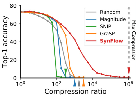
Figure 1: Layer-collapse leads to a sudden drop in accuracy. Top-1 test accuracy as a function of the compression ratio for a VGG-16 model pruned at initialization and trained on CIFAR100. Colored arrows represent the critical compression of the corresponding pruning algorithm. Only our algorithm, SynFlow, reaches the theoretical limit of max compression (black dashed line) without collapsing the network. See Sec. 7 for more details on the experiments.
图 1: 层坍塌导致准确率骤降。在CIFAR100数据集上,初始化剪枝后VGG-16模型在不同压缩比下的Top-1测试准确率。彩色箭头表示对应剪枝算法的临界压缩点。唯有我们的SynFlow算法能在不引发网络坍塌的情况下达到理论最大压缩极限(黑色虚线)。实验细节详见第7节。
Throughout this work, we benchmark our algorithm, SynFlow, against two simple baselines, random scoring and scoring based on weight magnitudes, as well as two state-of-the-art single-shot pruning algorithms, Single-shot Network Pruning based on Connection Sensitivity (SNIP) [13] and Gradient Signal Preservation (GraSP) [14]. SNIP [13] is a pioneering algorithm to prune neural networks at initialization by scoring weights based on the gradients of the training loss. GraSP [14] is a more recent algorithm that aims to preserve gradient flow at initialization by scoring weights based on the Hessian-gradient product. Both SNIP and GraSP have been thoroughly benchmarked by [14] against other state-of-the-art pruning algorithms that involve training [2, 35, 10, 11, 36, 21, 20], demonstrating competitive performance.
在本研究中,我们将算法SynFlow与两种简单基线(随机评分和基于权重幅度的评分)以及两种先进的一次性剪枝算法进行对比:基于连接敏感性的单次网络剪枝(SNIP) [13] 和梯度信号保留(GraSP) [14]。SNIP [13] 是一种开创性算法,通过基于训练损失梯度对权重评分,实现在初始化阶段剪枝神经网络。GraSP [14] 是较新的算法,通过基于海森-梯度积对权重评分,旨在保留初始化阶段的梯度流。[14] 已对SNIP和GraSP与其他需要训练的先进剪枝算法 [2, 35, 10, 11, 36, 21, 20] 进行了全面基准测试,证明了其具有竞争力的性能。
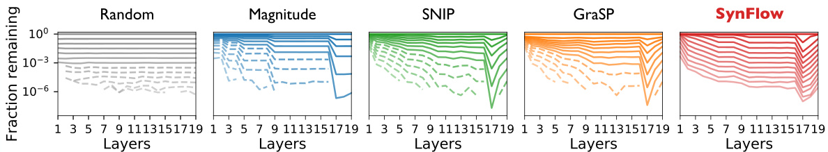
Figure 2: Where does layer-collapse occur? Fraction of parameters remaining at each layer of a VGG-19 model pruned at initialization with ImageNet over a range of compression ratios ( $10^{n}$ for $n=0,0.5,\ldots,6.0)$ . A higher transparency represents a higher compression ratio. A dashed line indicates that there is at least one layer with no parameters, implying layer-collapse has occurred.
图 2: 层坍塌发生在哪里?使用ImageNet在不同压缩比( $10^{n}$ ,其中 $n=0,0.5,\ldots,6.0$ )下初始化剪枝的VGG-19模型各层剩余参数比例。透明度越高表示压缩比越大。虚线表示至少存在一个无参数的层,即发生了层坍塌。
4 Conservation laws of synaptic saliency
4 突触显著性守恒定律
In this section, we will further verify that layer-collapse is a key obstacle to effective pruning at initialization and explore what is causing this failure mode. As shown in Fig. 2, with increasing compression ratios, existing random, magnitude, and gradient-based pruning algorithms will prematurely prune an entire layer making the network un trainable. Understanding why certain score metrics lead to layer-collapse is essential to improve the design of pruning algorithms.
在本节中,我们将进一步验证层坍塌 (layer-collapse) 是初始化阶段有效剪枝的关键障碍,并探究导致这种失效模式的原因。如图 2 所示,随着压缩比的增加,现有的随机剪枝、幅度剪枝和基于梯度的剪枝算法会过早地剪除整个网络层,导致网络无法训练。理解某些评分指标为何会导致层坍塌现象,对于改进剪枝算法设计至关重要。
Random pruning prunes every layer in a network by the same amount, evident by the horizontal lines in Fig. 2. With random pruning the smallest layer, the layer with the least parameters, is the first to be fully pruned. Conversely, magnitude pruning prunes layers at different rates, evident by the staircase pattern in Fig. 2. Magnitude pruning effectively prunes parameters based on the variance of their initialization, which for common network initialization s, such as Xavier [37] or Kaiming [38], are inversely proportional to the width of a layer [34]. With magnitude pruning the widest layers, the layers with largest input or output dimensions, are the first to be fully pruned. Gradient-based pruning algorithms SNIP [13] and GraSP [14] also prune layers at different rates, but it is less clear what the root cause for this preference is. In particular, both SNIP and GraSP aggressively prune the largest layer, the layer with the most trainable parameters, evident by the sharp peaks in Fig. 2. Based on this observation, we hypothesize that gradient-based scores averaged within a layer are inversely proportional to the layer size. We examine this hypothesis by constructing a theoretical framework grounded in flow networks. We first define a general class of gradient-based scores, prove a conservation law for these scores, and then use this law to prove that our hypothesis of inverse proportionality between layer size and average layer score holds exactly.
随机剪枝以相同比例剪枝网络中的每一层,如图2中的水平线所示。采用随机剪枝时,参数量最少的层会最先被完全剪除。相反,幅度剪枝以不同速率修剪各层,如图2中的阶梯模式所示。幅度剪枝根据参数初始化方差进行剪枝,对于Xavier [37] 或Kaiming [38] 等常见网络初始化方法,该方差与层宽度成反比 [34]。采用幅度剪枝时,输入或输出维度最大的宽层会最先被完全剪除。基于梯度的剪枝算法SNIP [13] 和GraSP [14] 同样以不同速率剪枝各层,但其偏好性成因尚不明确。值得注意的是,SNIP和GraSP会激进地剪除可训练参数量最多的层,如图2中的尖锐峰值所示。基于此现象,我们提出假设:层内平均梯度评分与层规模成反比。我们通过构建基于流网络的理论框架验证该假设,首先定义通用梯度评分类别,证明这些评分的守恒定律,进而利用该定律严格证明层规模与平均层评分呈反比的假设。
A general class of gradient-based scores. Synaptic saliency is a class of score metrics that can be expressed as the Hadamard product
基于梯度评分的通用类别。突触显著性 (synaptic saliency) 是一类可表示为Hadamard积的评分指标
$$
S(\theta)=\frac{\partial\mathcal{R}}{\partial\theta}\odot\theta,
$$
$$
S(\theta)=\frac{\partial\mathcal{R}}{\partial\theta}\odot\theta,
$$
where $\mathcal{R}$ is a scalar loss function of the output $y$ of a feed-forward network parameterized by $\theta$ . When $\mathcal{R}$ is the training loss $\mathcal{L}$ , the resulting synaptic saliency metric is equivalent (modulo sign) to $-\frac{\partial\mathcal{L}}{\partial\boldsymbol{\theta}}\odot\boldsymbol{\theta}$ the score metric used in Skeleton iz ation [1], one of the first network pruning algorithms. The resulting metric is also closely related to $\big|\frac{\partial\mathcal{L}}{\partial\theta}\odot\theta\big|$ the score used in SNIP [13], $\begin{array}{r}{-\left(H\frac{\partial\mathcal{L}}{\partial\theta}\right)\odot\theta}\end{array}$ the score used in GraSP, and $\left(\frac{\partial\mathcal{L}}{\partial\theta}\odot\theta\right)^{2}$ the scor e used in the pruning after training algorithm Taylor-FO [28]. When $\begin{array}{r}{\mathcal{R}=\langle\frac{\partial\mathcal{L}}{\partial y},y\rangle}\end{array}$ , the resulting synaptic saliency metric is closely related to $\mathrm{diag}(H)\theta\odot\theta$ , the score used in Optimal Brain Damage [2]. This general class of score metrics, while not encompassing, exposes key properties of gradient-based scores used for pruning.
其中$\mathcal{R}$是由参数$\theta$确定的前馈网络输出$y$的标量损失函数。当$\mathcal{R}$为训练损失$\mathcal{L}$时,所得突触显著性度量等价于(符号取反)剪枝算法Skeletonization[1]中使用的评分指标$-\frac{\partial\mathcal{L}}{\partial\boldsymbol{\theta}}\odot\boldsymbol{\theta}$。该指标也与SNIP[13]采用的$\big|\frac{\partial\mathcal{L}}{\partial\theta}\odot\theta\big|$、GraSP采用的$\begin{array}{r}{-\left(H\frac{\partial\mathcal{L}}{\partial\theta}\right)\odot\theta}\end{array}$,以及训练后剪枝算法Taylor-FO[28]采用的$\left(\frac{\partial\mathcal{L}}{\partial\theta}\odot\theta\right)^{2}$密切相关。当$\begin{array}{r}{\mathcal{R}=\langle\frac{\partial\mathcal{L}}{\partial y},y\rangle}\end{array}$时,所得突触显著性度量与Optimal Brain Damage[2]采用的$\mathrm{diag}(H)\theta\odot\theta$高度相关。这类评分指标虽未涵盖全部,但揭示了基于梯度的剪枝评分方法的关键特性。
The conservation of synaptic saliency. All synaptic saliency metrics respect two surprising conservation laws, which we prove in Appendix 9, that hold at any initialization and step in training.
突触显著性守恒。所有突触显著性指标都遵循两个令人惊讶的守恒定律(我们在附录9中予以证明),这些定律在训练的任何初始化和步骤中都成立。
Theorem 1. Neuron-wise Conservation of Synaptic Saliency. For a feed forward neural network with continuous, homogeneous activation functions, $\phi(x)=\phi^{\prime}(x)x,$ , (e.g. ReLU, Leaky ReLU, linear), $\begin{array}{r}{(\boldsymbol{S^{i n}}=\langle\frac{\tilde{\partial}\mathcal{R}}{\partial\theta^{i n}},\theta^{i\check{n}}\rangle)}\end{array}$ aisp teicq usaalli teon cthy ef osru tmh eo fi ntchoe msiynnga pptairc as male i teen rsc y( ifnocrl uthdie nog utthgeo ibniga sp) atro aam heitdedrse nf rnoemu rtohne hidden neuron $\begin{array}{r}{(S^{o u t}=\langle\frac{\partial\mathcal{R}}{\partial\theta^{o u t}},\theta^{o u t}\rangle)}\end{array}$
定理1. 神经元突触显著性守恒。对于一个具有连续、齐次激活函数的前馈神经网络,$\phi(x)=\phi^{\prime}(x)x$(例如ReLU、Leaky ReLU、线性函数),$\begin{array}{r}{(\boldsymbol{S^{i n}}=\langle\frac{\tilde{\partial}\mathcal{R}}{\partial\theta^{i n}},\theta^{i\check{n}}\rangle)}\end{array}$的输入突触显著性总和(包括偏置项)等于隐藏神经元$\begin{array}{r}{(S^{o u t}=\langle\frac{\partial\mathcal{R}}{\partial\theta^{o u t}},\theta^{o u t}\rangle)}\end{array}$的输出突触显著性。
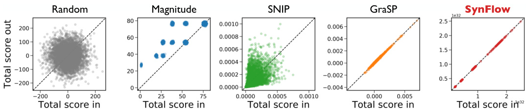
Figure 3: Neuron-wise conservation of score. Each dot represents a hidden unit from the featureextractor of a VGG-19 model pruned at initialization with ImageNet. The location of each dot corresponds to the total score for the unit’s incoming and outgoing parameters, $(S^{\mathrm{in}},S^{\mathrm{out}})$ . The black dotted line represents exact neuron-wise conservation of score.
图 3: 神经元级别的分数守恒。每个点代表VGG-19模型特征提取器中的一个隐藏单元,该模型在ImageNet数据集上初始化时进行了剪枝。点的位置对应于该单元输入和输出参数的总分数$(S^{\mathrm{in}},S^{\mathrm{out}})$。黑色虚线表示严格的神经元级别分数守恒。
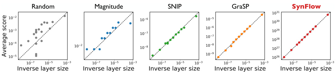
Figure 4: Inverse relationship between layer size and average layer score. Each dot represents a layer from a VGG-19 model pruned at initialization with ImageNet. The location of each dot corresponds to the layer’s average score4and inverse number of elements. The black dotted line represents a perfect linear relationship.
图 4: 层大小与平均层得分的反比关系。每个点代表使用ImageNet初始化剪枝的VGG-19模型中的一个层。点的位置对应该层的平均得分4与元素数量的倒数。黑色虚线表示完美的线性关系。
Theorem 2. Network-wise Conservation of Synaptic Saliency. The sum of the synaptic saliency across any set of parameters that exactly3 separates the input neurons $x$ from the output neurons y of a feed forward neural network with homogeneous activation functions equals $\begin{array}{r}{\langle\frac{\partial\mathcal{R}}{\partial x},\dot{x}\rangle=\langle\frac{\partial\mathcal{R}}{\partial y},y\rangle}\end{array}$ .
定理2: 网络突触显著性守恒。在前向神经网络中,对于任何能将输入神经元$x$与输出神经元$y$完全分离的参数集合,其突触显著性( Synaptic Saliency )之和满足$\begin{array}{r}{\langle\frac{\partial\mathcal{R}}{\partial x},\dot{x}\rangle=\langle\frac{\partial\mathcal{R}}{\partial y},y\rangle}\end{array}$,其中激活函数需满足齐次性条件。
For example, when considering a simple feed forward network with biases, then these conservation laws imply the non-trivial relationship: $\begin{array}{r}{\langle\frac{\partial\mathcal{R}}{\partial W^{[l]}},W^{[l]}\rangle+\sum_{i=l}^{L}\langle\frac{\partial\mathcal{R}}{\partial b^{[i]}},b^{[i]}\rangle=\langle\frac{\partial\mathcal{R}}{\partial y},y\rangle}\end{array}$ . Similar conservation properties have been noted in the network com plexity [39], implicit regular iz ation [40], and network interpret ability [41, 42] literature with some highlighting the potential applications to pruning [9, 43]. While the previous literatures have focused on attribution to the input pixels, or have ignored bias parameters, or have only considered the laws at the layer-level, we have formulated neuron-wise conservation laws that are more general and applicable to any parameter, including biases, in a network. Remarkably, these conservation laws of synaptic saliency apply to modern neural network architectures and a wide variety of neural network layers (e.g. dense, convolutional, pooling, residual) as visually demonstrated in Fig. 3. In Appendix 10 we discuss the specific setting of these conservation laws to parameters immediately preceding a batch normalization layer.
例如,考虑一个带偏置的简单前馈网络时,这些守恒定律蕴含着非平凡关系:$\begin{array}{r}{\langle\frac{\partial\mathcal{R}}{\partial W^{[l]}},W^{[l]}\rangle+\sum_{i=l}^{L}\langle\frac{\partial\mathcal{R}}{\partial b^{[i]}},b^{[i]}\rangle=\langle\frac{\partial\mathcal{R}}{\partial y},y\rangle}\end{array}$。类似守恒特性在网络复杂度 [39]、隐式正则化 [40] 和网络可解释性 [41, 42] 研究中已被注意到,部分研究强调了其在剪枝 [9, 43] 中的潜在应用。先前文献或聚焦于输入像素归因,或忽略偏置参数,或仅考虑层级守恒定律,而我们提出的神经元级守恒定律更具普适性,可应用于网络中包括偏置在内的任何参数。值得注意的是,这些突触显著性守恒定律适用于现代神经网络架构及多种网络层(如全连接层、卷积层、池化层、残差层),如图 3 直观所示。附录10将讨论这些守恒定律在批归一化层前参数中的具体设定。
Conservation and single-shot pruning leads to layer-collapse. The conservation laws of synaptic saliency provide us with the theoretical tools to validate our earlier hypothesis of inverse proportionality between layer size and average layer score as a root cause for layer-collapse of gradient-based pruning methods. Consider the set of parameters in a layer of a simple, fully connected neural network. This set would exactly separate the input neurons from the output neurons. Thus, by the network-wise conservation of synaptic saliency (theorem 2), the total score for this set is constant for all layers, implying the average is inversely proportional to the layer size. We can empirically evaluate this relationship at scale for existing pruning methods by computing the total score for each layer of a model, as shown in Fig. 4. While this inverse relationship is exact for synaptic saliency, other closely related gradient-based scores, such as the scores used in SNIP and GraSP, also respect this relationship. This validates the empirical observation that for a given compression ratio, gradient-based pruning methods will disproportionately prune the largest layers. Thus, if the compression ratio is large enough and the pruning score is only evaluated once, then a gradient-based pruning method will completely prune the largest layer leading to layer-collapse.
守恒性与单次剪枝导致层坍塌。突触显著性守恒定律为我们提供了理论工具,验证了我们先前关于层大小与平均层分数成反比这一假设——该假设正是基于梯度的剪枝方法产生层坍塌的根本原因。考虑一个简单全连接神经网络中某层的参数集合,该集合将精确分隔输入神经元与输出神经元。根据突触显著性的网络级守恒性(定理2),该集合的总分数对所有层都是恒定的,这意味着平均值与层大小成反比。如图4所示,我们可通过计算模型各层的总分数,对现有剪枝方法中的这种关系进行大规模实证评估。虽然这种反比关系在突触显著性中精确成立,但其他密切相关的基于梯度的分数(如SNIP和GraSP使用的分数)也遵循这一规律。这验证了以下实证观察:对于给定压缩比,基于梯度的剪枝方法会不成比例地剪除最大层。因此,若压缩比足够大且剪枝分数仅评估一次,基于梯度的剪枝方法将完全剪除最大层,从而导致层坍塌。
5 Magnitude pruning avoids layer-collapse with conservation and iteration
5 幅度剪枝通过守恒和迭代避免层坍塌
Having demonstrated and investigated the cause of layercollapse in single-shot pruning methods at initialization, we now explore an iterative pruning method that appears to avoid the issue entirely. Iterative Magnitude Pruning (IMP) is a recently proposed pruning algorithm that has proven to be successful in finding extremely sparse trainable neural networks at initialization (winning lottery tickets) [10, 11, 12, 44, 45, 46, 47]. The algorithm follows three simple steps. First train a network, second prune parameters with the smallest magnitude, third reset the unpruned parameters to their initialization and repeat until the desired compression ratio. While simple and powerful, IMP is impractical as it involves training the network several times, essentially defeating the purpose of constructing a sparse initialization. That being said it does not suffer from the same catastrophic layer-collapse that other pruning at initialization methods are susceptible to. Thus, understanding better how IMP avoids layer-collapse might shed light on how to improve pruning at initialization.
在单次剪枝方法中已经展示并研究了初始化时层坍塌的成因,我们现在探索一种似乎能完全避免该问题的迭代剪枝方法。迭代幅度剪枝(IMP)是近期提出的一种剪枝算法,已被证明能成功在初始化阶段找到极稀疏的可训练神经网络(中奖彩票)[10, 11, 12, 44, 45, 46, 47]。该算法遵循三个简单步骤:首先训练网络,其次剪除幅度最小的参数,最后将未剪枝参数重置为初始值并重复直至达到目标压缩率。虽然简单高效,但IMP需要多次训练网络,本质上违背了构建稀疏初始化的初衷,因此并不实用。不过它确实不会像其他初始化剪枝方法那样遭受灾难性的层坍塌问题。因此,深入理解IMP如何避免层坍塌,可能为改进初始化剪枝提供启示。
As has been noted previously [10, 11], iteration is essential for stabilizing IMP. In fact, without sufficient pruning iterations, IMP will suffer from layer-collapse, evident in the sudden accuracy drops for the darker curves in Fig. 5a. However, the number of pruning iterations alone cannot explain IMP’s success at avoiding layer-collapse. Notice that if IMP didn’t train the network during each prune cycle, then, no matter the number of pruning iterations, it would be equivalent to single-shot magnitude pruning. Thus, something very critical must happen to the magnitude of the parameters during training, that when coupled (b) IMP obtains conservation by training
此前已有研究指出 [10, 11],迭代对于稳定迭代式剪枝(IMP)至关重要。实际上,若剪枝迭代次数不足,IMP会出现层坍塌现象,图5a中颜色较深的曲线突然下跌的精度值便印证了这一点。但仅凭剪枝迭代次数并不能解释IMP成功避免层坍塌的原因。值得注意的是,若IMP在每个剪枝周期中不训练网络,那么无论进行多少次剪枝迭代,其效果都将等同于单次幅度剪枝。因此,参数幅度在训练过程中必然发生了某些关键性变化,当这些变化与(b) IMP通过训练获得守恒性相结合时...
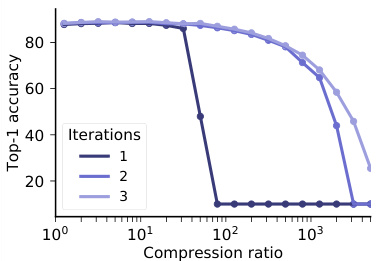
图 1:
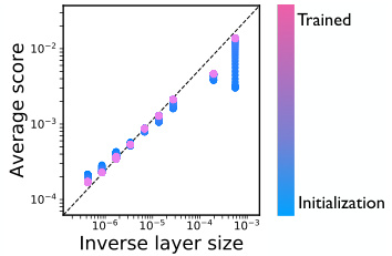
(a) Iteration is needed to avoid layer-collapse Figure 5: How IMP avoids layer collapse. (a) Multiple iterations of trainingpruning cycles is needed to prevent IMP from suffering layer-collapse. (b) The average square magnitude scores per layer, originally at initialization (blue), converge through training towards a linear relationship with the inverse layer size after training (pink), suggesting layer-wise conservation. All data is from a VGG-19 model trained on CIFAR-10.
图 5: IMP如何避免层坍塌。(a) 需要多次训练-剪枝循环迭代来防止IMP出现层坍塌。(b) 每层平均平方幅度分数在初始化时(蓝色)通过训练逐渐收敛至与逆层尺寸呈线性关系(粉色),表明存在层级守恒现象。所有数据均来自在CIFAR-10上训练的VGG-19模型。
with sufficient pruning iterations allows IMP to avoid layer-collapse. We hypothesize that gradient descent training effectively encourages the scores to observe an approximate layer-wise conservation law, which when coupled with sufficient pruning iterations allows IMP to avoid layer-collapse.
通过足够的剪枝迭代次数,IMP能够避免层级坍塌。我们假设梯度下降训练能有效促使分数遵循近似的层级守恒定律,当结合足够的剪枝迭代时,这一机制使IMP得以规避层级坍塌问题。
Gradient descent encourages conservation. To better understand the dynamics of the IMP algorithm during training, we will consider a differentiable score $\begin{array}{r}{S(\theta_{i})=\frac{1}{2}\theta_{i}^{2}}\end{array}$ algorithmic ally equivalent to the magnitude score. Consider these scores throughout training with gradient descent on a loss function $\mathcal{L}$ using an infinitesimal step size (i.e. gradient flow). In this setting, the temporal derivative of the parameters is equivalent to $\begin{array}{r}{{\frac{d\theta}{d t}}=-{\frac{\stackrel{\cdot}{\partial}\mathcal{L}}{\partial\theta}}}\end{array}$ − ∂∂θL , and thus the temporal derivative of the score is $\begin{array}{r}{\frac{d}{d t}\frac{1}{2}\theta_{i}^{2}=\frac{d\theta_{i}}{d t}\odot\theta_{i}=-\frac{\partial\mathcal{L}}{\partial\theta_{i}}\odot\theta_{i}}\end{array}$ . Surprisingly, this is a form of synaptic saliency and thus the neuron-wise and layer-wise conservation laws from Sec. 4 apply. In particular, this implies that for any two layers $l$ and $k$ of a simple, fully connected network, then $\begin{array}{r}{\frac{d}{d t}||W^{[l]}||_ {F}^{2}=\frac{d}{d t}||\bar{W^{[k]}}||_{F}^{2}}\end{array}$ . This invariance has been noticed before by [40] as a form of implicit regular iz ation and used to explain the empirical phenomenon that trained multi-layer models can have similar layer-wise magnitudes. In the context of pruning, this phenomenon implies that gradient descent training, with a small enough learning rate, encourages the squared magnitude scores to converge to an approximate layer-wise conservation, as shown in Fig. 5b.
梯度下降促进守恒性。为了更好地理解训练过程中IMP算法的动态特性,我们将考虑一个可微分评分函数$\begin{array}{r}{S(\theta_{i})=\frac{1}{2}\theta_{i}^{2}}\end{array}$,该函数在算法上等效于幅度评分。考察使用无穷小步长(即梯度流)对损失函数$\mathcal{L}$进行梯度下降训练时这些评分的变化。在此设定下,参数的时间导数等价于$\begin{array}{r}{{\frac{d\theta}{d t}}=-{\frac{\stackrel{\cdot}{\partial}\mathcal{L}}{\partial\theta}}}\end{array}$,因此评分的时间导数为$\begin{array}{r}{\frac{d}{d t}\frac{1}{2}\theta_{i}^{2}=\frac{d\theta_{i}}{d t}\odot\theta_{i}=-\frac{\partial\mathcal{L}}{\partial\theta_{i}}\odot\theta_{i}\end{array}$。值得注意的是,这实际上是突触显著性的一种形式,因此第4节中的神经元级和层级守恒定律同样适用。特别地,这意味着对于简单全连接网络的任意两个层$l$和$k$,有$\begin{array}{r}{\frac{d}{d t}||W^{[l]}||_ {F}^{2}=\frac{d}{d t}||\bar{W^{[k]}}||_{F}^{2}\end{array}$。[40]曾注意到这种不变性是一种隐式正则化形式,并用其解释训练后的多层模型可能具有相似层级幅值的经验现象。在剪枝背景下,该现象表明只要学习率足够小,梯度下降训练会促使平方幅度评分收敛至近似层级守恒状态,如图5b所示。
Conservation and iterative pruning avoids layer-collapse. As explained in section 4, conservation alone leads to layer-collapse by assigning parameters in the largest layers with lower scores relative to parameters in smaller layers. However, if conservation is coupled with iterative pruning, then when the largest layer is pruned, becoming smaller, then in subsequent iterations the remaining parameters of this layer will be assigned higher relative scores. With sufficient iterations, conservation coupled with iteration leads to a self-balancing pruning strategy allowing IMP to avoid layer-collapse. This insight on the importance of conservation and iteration applies more broadly to other algorithms with exact or approximate conservation properties. Indeed, concurrent work empirically confirms that iteration improves the performance of SNIP [48, 49].
守恒与迭代剪枝避免层级塌缩。如第4节所述,仅采用守恒机制会因给大层参数分配相对低于小层参数的分数而导致层级塌缩。但若将守恒与迭代剪枝结合,当最大层被剪枝变小时,在后续迭代中该层剩余参数将获得更高的相对分数。经过足够迭代后,守恒与迭代的结合形成自平衡剪枝策略,使IMP得以规避层级塌缩。这一关于守恒与迭代重要性的洞见,同样适用于其他具有精确或近似守恒特性的算法。事实上,同期研究已实证表明迭代能提升SNIP算法的性能 [48, 49]。
6 A data-agnostic algorithm satisfying Maximal Critical Compression
6 满足最大关键压缩的数据无关算法
In the previous section we identified two key ingredients of IMP’s ability to avoid layer-collapse: (i) approximate layer-wise conservation of the pruning scores, and (ii) the iterative re-evaluation of these scores. While these properties allow the IMP algorithm to identify high performing and highly sparse, trainable neural networks, it requires an impractical amount of computation to obtain them. Thus, we aim to construct a more efficient pruning algorithm while still inheriting the key aspects of IMP’s success. So what are the essential ingredients for a pruning algorithm to avoid layer-collapse and provably attain Maximal Critical Compression? We prove the following theorem in Appendix 9.
在前一节中,我们确定了IMP方法避免层坍塌的两个关键要素:(i) 剪枝分数的近似逐层守恒性,以及(ii) 对这些分数的迭代重评估。虽然这些特性使得IMP算法能够识别出高性能、高稀疏度且可训练的神经网络,但获取它们需要大量不切实际的计算。因此,我们的目标是构建一种更高效的剪枝算法,同时仍继承IMP成功的关键要素。那么,剪枝算法要避免层坍塌并理论上达到最大临界压缩(Maximal Critical Compression)的关键要素是什么?我们在附录9中证明了以下定理。
Theorem 3. Iterative, positive, conservative scoring achieves Maximal Critical Compression. If a pruning algorithm, with global-masking, assigns positive scores that respect layer-wise conservation and if the prune size, the total score for the parameters pruned at any iteration, is strictly less than the cut size, the total score for an entire layer, whenever possible, then the algorithm satisfies the Maximal Critical Compression axiom.
定理3: 迭代式、正向、保守的评分可实现最大关键压缩。若采用全局掩码的剪枝算法分配的评分满足层间守恒性,且剪枝规模(即每次迭代被剪参数总评分)始终严格小于临界规模(即单层总评分),则该算法满足最大关键压缩公理。
The Iterative Synaptic Flow Pruning (SynFlow) algorithm. Theorem 3 directly motivates the design of our novel pruning algorithm, SynFlow, that provably reaches Maximal Critical Compression. First, the necessity for iterative score evaluation discourages algorithms that involve back propagation on batches of data, and instead motivates the development of an efficient data-independent scoring procedure. Second, positivity and conservation motivates the construction of a loss function that yields positive synaptic saliency scores. We combine these insights to introduce a new loss function (where $\mathbb{1}$ is the all ones vector and $\left\vert\theta^{[l]}\right\vert$ is the element-wise absolute value of parameters in the $l^{\mathrm{th}}$ layer),
迭代突触流剪枝(SynFlow)算法。定理3直接启发我们设计出新型剪枝算法SynFlow,该算法可证明达到最大临界压缩。首先,迭代评分计算的必要性排除了基于数据批次反向传播的算法,转而促使我们开发一种高效的数据无关评分流程。其次,正值性与守恒性要求我们构建能产生正突触显著性评分的损失函数。结合这些洞见,我们提出新损失函数(其中$\mathbb{1}$为全1向量,$\left\vert\theta^{[l]}\right\vert$表示第$l^{\mathrm{th}}$层参数的逐元素绝对值),
$$
\mathcal{R}_ {\mathrm{SF}}=\mathbb{1}^{T}\left(\prod_{l=1}^{L}|\theta^{[l]}|\right)\mathbb{1}
$$
$$
\mathcal{R}_ {\mathrm{SF}}=\mathbb{1}^{T}\left(\prod_{l=1}^{L}|\theta^{[l]}|\right)\mathbb{1}
$$
that yields the positive, synaptic saliency scores $(\frac{\partial\mathcal{R}_{\mathrm{SE}}}{\partial\theta}\odot\theta)$ we term Synaptic Flow. For a simple, fully connected network (i.e. $f(x)=W^{[{N}]}\cdot\cdot\cdot W^{[{1}]}x)$ , we can factor the Synaptic Flow score for a parameter w[ilj] as
产生正向突触显著性分数 $(\frac{\partial\mathcal{R}_{\mathrm{SE}}}{\partial\theta}\odot\theta)$ 的方法,我们称之为突触流 (Synaptic Flow) 。对于一个简单的全连接网络 (即 $f(x)=W^{[{N}]}\cdot\cdot\cdot W^{[{1}]}x)$ ,我们可以将参数 w[ilj] 的突触流分数分解为
$$
S_{\mathrm{SF}}(w_{i j}^{[l]})=\left[\mathbb{1}^{\top}\prod_{k=l+1}^{N}\Big|W^{[k]}\Big|\right]_ {i}\left|w_{i j}^{[l]}\right|\left[\prod_{k=1}^{l-1}\Big|W^{[k]}\Big|\mathbb{1}\right]_{j}.
$$
$$
S_{\mathrm{SF}}(w_{i j}^{[l]})=\left[\mathbb{1}^{\top}\prod_{k=l+1}^{N}\Big|W^{[k]}\Big|\right]_ {i}\left|w_{i j}^{[l]}\right|\left[\prod_{k=1}^{l-1}\Big|W^{[k]}\Big|\mathbb{1}\right]_{j}.
$$
This perspective demonstrates that Synaptic Flow score is a generalization of magnitude score $(|w_{i j}^{[l]}|)$ , where the scores consider the product of synaptic strengths flowing through each parameter, taking the inter-layer interactions of parameters into account. In fact, this more generalized magnitude has been discussed previously in literature as a path-norm [50]. The Synaptic Flow loss, equation (2), is the $l_{1}$ -path norm of a network and the synaptic flow score for a parameter is the portion of the norm through the parameter. We use the Synaptic Flow score in the Iterative Synaptic Flow Pruning (SynFlow) algorithm summarized in the pseudocode below.
这一观点表明,突触流评分 (Synaptic Flow score) 是幅度评分 $(|w_{i j}^{[l]}|)$ 的广义形式,该评分通过考虑流经每个参数的突触强度乘积,将参数间的跨层交互纳入考量。事实上,这种更广义的幅度在文献[50]中已被讨论为路径范数 (path-norm)。突触流损失函数(公式(2))即网络的 $l_{1}$ -路径范数,而参数的突触流评分则是该范数流经该参数的部分。我们在下方伪代码总结的迭代突触流剪枝 (SynFlow) 算法中使用了突触流评分。
Given a network $f(x;\theta_{0})$ and specified compression ratio $\rho$ , the SynFlow algorithm requires only one additional hyper parameter, the number of pruning iterations $n$ . We demonstrate in Appendix 12, that an exponential pruning schedule $(\rho^{-k/n})$ with $n=100$ pruning iterations essentially prevents layer-collapse whenever avoidable (Fig. 1), while remaining computationally feasible, even for large networks.
给定网络 $f(x;\theta_{0})$ 和指定的压缩比 $\rho$ ,SynFlow算法仅需一个额外的超参数——剪枝迭代次数 $n$ 。我们在附录12中证明,采用指数剪枝调度 $(\rho^{-k/n})$ 配合 $n=100$ 次迭代时,该算法能在可避免的情况下有效防止层坍塌 (如图1所示) ,同时即使对于大型网络也保持计算可行性。
Computational cost of SynFlow. The computational cost of a pruning algorithm can be measured by the number of forward/backward passes (#iterations $\times$ #examples per iteration). We always run the data-agnostic SynFlow with 100 iterations, implying it takes 100 passes no matter the dataset. SNIP and GraSP each involve one iteration, but use ten times the number of classes per iteration requiring 1000, 2000, and 10,000 passes for CIFAR-100, Tiny-ImageNet, and ImageNet respectively.
SynFlow的计算成本。剪枝算法的计算成本可以通过前向/反向传播的次数(#迭代次数 $\times$ 每次迭代的样本数)来衡量。数据无关的SynFlow始终以100次迭代运行,这意味着无论数据集如何都需要100次传播。SNIP和GraSP各涉及一次迭代,但每次迭代使用类别数的十倍样本量,因此在CIFAR-100、Tiny-ImageNet和ImageNet上分别需要1000、2000和10,000次传播。
7 Experiments
7 实验
We empirically benchmark the performance of our algorithm, SynFlow (red), against the baselines random pruning and magnitude pruning, as well as the state-of-the-art algorithms SNIP [13] and GraSP [14]. In Fig. 6, we test the five algorithms on 12 distinct combinations of modern architectures (VGG-11, VGG-16, ResNet-18, WideResNet-18) and datasets (CIFAR-10, CIFAR-100, Tiny ImageNet) over an exponential sweep of compression ratios ( $10^{\alpha}$ for $\alpha=[0,0.25,\ldots,3.75,4],$ ). See Appendix 13 for more details and hyper parameters of the experiments. Consistently, SynFlow outperforms the other algorithms in the high compression regime $(\mathrm{\bar{1}0^{1.5}}<\rho)$ and demonstrates more stability, as indicated by its tight intervals. SynFlow is also quite competitive in the low compression regime $(\rho<10^{1.5})$ ). Although SNIP and GraSP can partially outperform SynFlow in this regime, both methods suffer from layer-collapse as indicated by their sharp drops in accuracy.
我们通过实验将算法SynFlow(红色)与基线方法随机剪枝和幅度剪枝,以及前沿算法SNIP[13]和GraSP[14]进行性能对比。在图6中,我们在12种不同组合的现代架构(VGG-11、VGG-16、ResNet-18、WideResNet-18)和数据集(CIFAR-10、CIFAR-100、Tiny ImageNet)上,以指数级压缩比($10^{\alpha}$,其中$\alpha=[0,0.25,\ldots,3.75,4]$)测试了这五种算法。实验详细设置和超参数参见附录13。在高压缩比区域$(\mathrm{\bar{1}0^{1.5}}<\rho)$下,SynFlow始终优于其他算法,并展现出更稳定的性能(表现为紧密的置信区间)。在低压缩比区域$(\rho<10^{1.5})$下,SynFlow也极具竞争力。虽然SNIP和GraSP在该区域可能部分优于SynFlow,但这两种方法都存在层坍塌问题(表现为准确率急剧下降)。
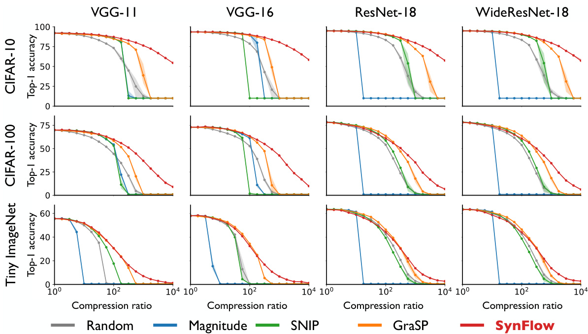
Figure 6: SynFlow consistently outperforms other pruning methods in high compression regimes avoiding layer collapse. Top-1 test accuracy as a function of different compression ratios over 12 distinct combinations of models and datasets. We performed three runs with the same hyper parameter conditions and different random seeds. The solid line represents the mean, the shaded region represents area between minimum and maximum performance of the three runs.
图 6: SynFlow在高压缩率下始终优于其他剪枝方法,避免了层坍塌。Top-1测试准确率随12种不同模型和数据集组合的压缩比变化情况。我们在相同超参数条件和不同随机种子下进行了三次实验,实线表示平均值,阴影区域表示三次实验的最小和最大性能范围。
Comparing to expensive iterative pruning algorithms. Theorem 3 states that iteration is a necessary ingredient for any pruning algorithm, elucidating the success of iterative magnitude pruning and concurrent work on iterative versions of SNIP [48, 49]. As shown in Fig. 7, iteration helps SNIP avoid early layer-collapse, but with a multiplicative computational cost. Additionally, these iterative versions of SNIP still suffer from layer-collapse, long before reaching max compression, which SynFlow is provably guaranteed to reach.
与昂贵的迭代剪枝算法相比,定理3表明迭代是所有剪枝算法的必要组成部分,这解释了迭代幅度剪枝的成功以及SNIP [48, 49] 迭代版本的相关研究。如图7所示,迭代帮助SNIP避免了早期层坍塌,但会带来乘法级的计算成本。此外,这些SNIP的迭代版本在达到最大压缩率之前仍会出现层坍塌现象,而SynFlow则被证明能确保达到该极限。
Ablation studies. The SynFlow algorithm demonstrates that we do not need to use data to match, and at times outperform, data-dependent pruning methods at initialization such as SNIP and GraSP. This result challenges the effectiveness of how existing algorithms use data at initialization, and provides a concrete algorithmic baseline that any future algorithms that prune at initialization using data should surpass. A recent follow-up work [51] confirms our observation that SynFlow is competitive with SNIP and GraSP even in the low-compression regime and for large-scale datasets (ImageNet) and models (ResNet-50). This work also performs careful ablation studies that offer concrete evidence supporting the theoretical motivation for SynFlow and insightful observations for further improvements of the algorithm. See Appendix 11 for a more detailed discussion on these ablation studies presented in [51].
消融研究。SynFlow算法表明,我们无需使用数据就能在初始化阶段达到甚至超越SNIP和GraSP等依赖数据的剪枝方法。这一结果挑战了现有算法在初始化阶段使用数据的有效性,并为未来所有基于数据初始剪枝的算法提供了必须超越的具体算法基线。近期后续研究[51]证实了我们的发现:即使在低压缩率场景下,针对大规模数据集(ImageNet)和模型(ResNet-50),SynFlow仍能与SNIP和GraSP保持竞争力。该研究还进行了细致的消融实验,为SynFlow的理论动机提供了实证支持,并为算法改进提出了深刻见解。关于[51]中这些消融研究的详细讨论,请参阅附录11。
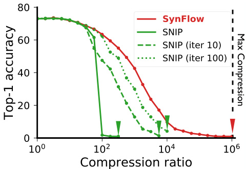
Figure 7: Iteration improves SNIP, but layer-collapse still occurs. Top1 test accuracy as a function of the compression ratio for a VGG-16 model pruned at initialization and trained on CIFAR-100.
图 7: 迭代优化能提升SNIP (Sparse Neural Network Pruning) 效果,但层坍塌现象仍存在。展示了在CIFAR-100数据集上初始化剪枝并训练的VGG-16模型,其Top1测试准确率随压缩比变化的函数关系。
8 Conclusion
8 结论
In this paper, we developed a unifying theoretical framework that explains why existing pruning algorithms at initialization suffer from layer-collapse. We applied our framework to elucidate how iterative magnitude pruning [10] overcomes layer-collapse to identify winning lottery tickets at initi aliz ation. Building on the theory, we designed a new data-agnostic pruning algorithm, SynFlow, that provably avoids layer-collapse and reaches Maximal Critical Compression. Finally, we empirically confirmed that our SynFlow algorithm consistently matches or outperforms existing algorithms across 12 distinct combinations of models and datasets, despite the fact that our algorithm is data-agnostic and requires no pre-training. Promising future directions for this work are to (i) explore a larger space of potential pruning algorithms that satisfy Maximal Critical Compression, (ii) harness SynFlow as an efficient way to compute appropriate per-layer compression ratios to combine with existing scoring metrics, and (iii) incorporate pruning as a part of neural network initialization schemes. Overall, our data-agnostic pruning algorithm challenges the existing paradigm that data must be used, at initialization, to quantify which synapses of a neural network are important.
本文提出了一个统一的理论框架,用于解释现有初始化剪枝算法为何会出现层坍塌问题。我们应用该框架阐明了迭代幅度剪枝[10]如何在初始化阶段克服层坍塌现象并识别中奖彩票。基于该理论,我们设计了一种新的数据无关剪枝算法SynFlow,该算法可证明避免层坍塌并达到最大临界压缩率。最后,我们通过实验验证了SynFlow算法在12种不同模型和数据集组合中始终匹配或超越现有算法,尽管该算法完全不需要数据且无需预训练。未来研究方向包括:(i) 探索满足最大临界压缩率的更大剪枝算法空间,(ii) 利用SynFlow作为计算各层合适压缩比的高效方法,与现有评分指标相结合,(iii) 将剪枝作为神经网络初始化方案的一部分。总体而言,我们的数据无关剪枝算法挑战了现有范式——必须在初始化阶段使用数据来量化神经网络突触的重要性。
Broader Impact
更广泛的影响
Neural network pruning has the potential to increase the energy efficiency of neural network models and decrease the environmental impact of their training. It also has the potential to allow for trained neural network models to be more easily deployed on edge devices such as mobile phones. Our work explores neural network pruning mainly from a theoretical angle and thus these impacts are not directly applicable to our work. However, future work might be able to realize these potentials and thus must consider their impacts more carefully.
神经网络剪枝技术有望提升神经网络模型的能效,并降低其训练过程对环境的影响。该技术还可能使训练好的神经网络模型更易于部署在手机等边缘设备上。本研究主要从理论角度探索神经网络剪枝,因此这些影响并不直接适用于我们的工作。然而,未来的研究或许能够实现这些潜力,因而需要更审慎地考量其影响。
Acknowledgments and Disclosure of Funding
致谢与资金披露
We thank Jonathan M. Bloom, Weihua Hu, Javier Sagastuy-Brena, Chaoqi Wang, Guodong Zhang, Chengxu Zhuang, and members of the Stanford Neuroscience and Artificial Intelligence Laboratory for helpful discussions. We thank the Stanford Data Science Scholars program (DK), the Burroughs Wellcome, Simons and James S. McDonnell foundations, and an NSF career award (SG) for support. This work was funded in part by the IBM-Watson AI Lab. D.L.K.Y is supported by the McDonnell Foundation (Understanding Human Cognition Award Grant No. 220020469), the Simons Foundation (Collaboration on the Global Brain Grant No. 543061), the Sloan Foundation (Fellowship FG-2018- 10963), the National Science Foundation (RI 1703161 and CAREER Award 1844724), the DARPA Machine Common Sense program, and hardware donation from the NVIDIA Corporation.
我们感谢Jonathan M. Bloom、Weihua Hu、Javier Sagastuy-Brena、Chaoqi Wang、Guodong Zhang、Chengxu Zhuang以及斯坦福神经科学与人工智能实验室成员的宝贵讨论。感谢斯坦福数据科学学者项目(DK)、Burroughs Wellcome基金会、Simons基金会、James S. McDonnell基金会以及美国国家科学基金会(NSF)职业奖(SG)的支持。本研究部分由IBM-Watson AI实验室资助。D.L.K.Y的研究获得了McDonnell基金会(人类认知理解奖220020469)、Simons基金会(全球大脑合作项目543061)、Sloan基金会(FG-2018-10963)、美国国家科学基金会(RI 1703161和CAREER奖1844724)、DARPA机器常识项目以及NVIDIA公司的硬件捐赠支持。
References
参考文献
[30] Xin Dong, Shangyu Chen, and Sinno Pan. Learning to prune deep neural networks via layerwise optimal brain surgeon. In Advances in Neural Information Processing Systems, pages 4857–4867, 2017.
[30] Xin Dong, Shangyu Chen, Sinno Pan. 基于层级最优脑外科手术的深度神经网络剪枝学习. 收录于《神经信息处理系统进展》, 第4857-4867页, 2017年.
Appendix
附录
9 Proofs
9 证明
Theorem 1. Neuron-wise Conservation of Synaptic Saliency. For a feed forward neural network with continuous, homogeneous activation functions, $\phi(x)=\phi^{\prime}(x)x$ , (e.g. ReLU, Leaky ReLU, linear), the sum of the synaptic saliency for the incoming parameters (including the bias) to a hidden neuron $\begin{array}{r}{(\boldsymbol{S^{\mathrm{in}}}=\langle\frac{\partial\mathcal{R}}{\partial\theta^{\mathrm{in}}},\theta^{\mathrm{in}}\rangle)}\end{array}$ is equal to the sum of the synaptic saliency for the outgoing parameters from the hidden neuron $\begin{array}{r}{(S^{\mathrm{out}}=\langle\frac{\partial\mathcal{R}}{\partial\theta^{\mathrm{out}}},\theta^{\mathrm{out}}\rangle)}\end{array}$ .
定理1. 神经元突触显著性的守恒性。对于一个具有连续、齐次激活函数的前馈神经网络,$\phi(x)=\phi^{\prime}(x)x$(例如ReLU、Leaky ReLU、线性函数),隐藏神经元输入参数(包括偏置)的突触显著性之和 $\begin{array}{r}{(\boldsymbol{S^{\mathrm{in}}}=\langle\frac{\partial\mathcal{R}}{\partial\theta^{\mathrm{in}}},\theta^{\mathrm{in}}\rangle)\end{array}$ 等于该隐藏神经元输出参数的突触显著性之和 $\begin{array}{r}{(S^{\mathrm{out}}}=\langle\frac{\partial\mathcal{R}}{\partial\theta^{\mathrm{out}}},\theta^{\mathrm{out}}\rangle)\end{array}$。
Proof. Consider the $j^{\mathrm{th}}$ hidden neuron of a network with outgoing parameters $\theta_{i j}^{\mathrm{out}}$ and incoming parameters $\theta_{j k}^{\mathrm{in}}$ , such that $\begin{array}{r}{\frac{\partial\mathcal{R}}{\partial\phi(z_{j})}=\sum_{i}\frac{\partial\mathcal{R}}{\partial z_{i}}\theta_{i j}^{\mathrm{out}}}\end{array}$ and $\begin{array}{r}{z_{j}=\sum_{k}\theta_{j k}^{\mathrm{in}}\phi(z_{k})}\end{array}$ where there exists a bias parameter $\theta_{b}^{\mathrm{in}}=b_{j}$ and a neuron in each layer with the activation $\phi_{b}=1$ . The sum of the synaptic saliency for the outgoing parameters is
证明。考虑一个网络的第 $j^{\mathrm{th}}$ 个隐藏神经元,其传出参数为 $\theta_{i j}^{\mathrm{out}}$,传入参数为 $\theta_{j k}^{\mathrm{in}}$,使得 $\begin{array}{r}{\frac{\partial\mathcal{R}}{\partial\phi(z_{j})}=\sum_{i}\frac{\partial\mathcal{R}}{\partial z_{i}}\theta_{i j}^{\mathrm{out}}}\end{array}$ 且 $\begin{array}{r}{z_{j}=\sum_{k}\theta_{j k}^{\mathrm{in}}\phi(z_{k})}\end{array}$,其中存在一个偏置参数 $\theta_{b}^{\mathrm{in}}=b_{j}$,以及每层中有一个神经元的激活函数为 $\phi_{b}=1$。传出参数的突触显著性和为
$$
S^{\mathrm{out}}=\sum_{i}\frac{\partial\mathcal{R}}{\partial\theta_{i j}^{\mathrm{out}}}\theta_{i j}^{\mathrm{out}}=\sum_{i}\frac{\partial\mathcal{R}}{\partial z_{i}}\phi(z_{j})\theta_{i j}^{\mathrm{out}}=\left(\sum_{i}\frac{\partial\mathcal{R}}{\partial z_{i}}\theta_{i j}^{\mathrm{out}}\right)\phi(z_{j})=\frac{\partial\mathcal{R}}{\partial\phi(z_{j})}\phi(z_{j}).
$$
$$
S^{\mathrm{out}}=\sum_{i}\frac{\partial\mathcal{R}}{\partial\theta_{i j}^{\mathrm{out}}}\theta_{i j}^{\mathrm{out}}=\sum_{i}\frac{\partial\mathcal{R}}{\partial z_{i}}\phi(z_{j})\theta_{i j}^{\mathrm{out}}=\left(\sum_{i}\frac{\partial\mathcal{R}}{\partial z_{i}}\theta_{i j}^{\mathrm{out}}\right)\phi(z_{j})=\frac{\partial\mathcal{R}}{\partial\phi(z_{j})}\phi(z_{j}).
$$
The sum of the synaptic saliency for the incoming parameters is
传入参数的突触显著性总和
$$
S^{\mathrm{in}}=\sum_{k}\frac{\partial\mathcal{R}}{\partial\theta_{j k}^{\mathrm{in}}}\theta_{j k}^{\mathrm{in}}=\sum_{k}\frac{\partial\mathcal{R}}{\partial z_{j}}\phi(z_{k})\theta_{j k}^{\mathrm{in}}=\frac{\partial\mathcal{R}}{\partial z_{j}}\left(\sum_{k}\theta_{j k}^{\mathrm{in}}\phi(z_{k})\right)=\frac{\partial\mathcal{R}}{\partial z_{j}}z_{j}.
$$
$$
S^{\mathrm{in}}=\sum_{k}\frac{\partial\mathcal{R}}{\partial\theta_{j k}^{\mathrm{in}}}\theta_{j k}^{\mathrm{in}}=\sum_{k}\frac{\partial\mathcal{R}}{\partial z_{j}}\phi(z_{k})\theta_{j k}^{\mathrm{in}}=\frac{\partial\mathcal{R}}{\partial z_{j}}\left(\sum_{k}\theta_{j k}^{\mathrm{in}}\phi(z_{k})\right)=\frac{\partial\mathcal{R}}{\partial z_{j}}z_{j}.
$$
When $\phi$ is homogeneous, then $\begin{array}{r}{\frac{\partial\mathcal{R}}{\partial\phi(z_{j})}\phi(z_{j})=\frac{\partial\mathcal{R}}{\partial z_{j}}z_{j}}\end{array}$
当 $\phi$ 是齐次函数时,$\begin{array}{r}{\frac{\partial\mathcal{R}}{\partial\phi(z_{j})}\phi(z_{j})=\frac{\partial\mathcal{R}}{\partial z_{j}}z_{j}}\end{array}$
Theorem 2. Network-wise Conservation of Synaptic Saliency. The sum of the synaptic saliency across any set of parameters that exactly separates the input neurons $x$ from the output neurons y of a feed forward neural network with homogeneous activation functions equals ⟨ ∂∂xR , x⟩ = ⟨ ∂∂yR , y⟩.
定理2:网络层面的突触显著性守恒。在具有齐次激活函数的前馈神经网络中,任何将输入神经元$x$与输出神经元y精确分离的参数集上的突触显著性之和等于⟨∂R/∂x, x⟩ = ⟨∂R/∂y, y⟩。
Proof. We begin by defining the set of neurons $(V)$ and the set of prunable parameters $(E)$ for a neural network.
证明。我们首先定义神经网络中的神经元集合 $(V)$ 和可修剪参数集合 $(E)$。
Consider a subset of the neurons $S\subset V$ , such that all output neurons $y_{c}\in S$ and all input neurons $x_{i}\in V\backslash S$ . Consider the set of parameters cut by this partition
考虑神经元子集 $S\subset V$,使得所有输出神经元 $y_{c}\in S$ 且所有输入神经元 $x_{i}\in V\backslash S$。考虑由该划分切割的参数集
$$
C(S)={\theta_{u v}\in E:u\in S,v\in V\backslash S}.
$$
$$
C(S)={\theta_{u v}\in E:u\in S,v\in V\backslash S}.
$$
By theorem 1, we know that that sum of the synaptic saliency over $C(S)$ is equal to the sum of the synaptic saliency over the set of parameters adjacent to $C(S)$ and between neurons in $S$ , ${\theta_{t u}\in E:t\in S,u\in\partial S}$ . Continuing this argument, then eventually we get that this sum must be equal to the sum of the synaptic saliency over the set of parameters incident to the output neurons $y$ , which is
根据定理1,我们知道 $C(S)$ 上的突触显著性之和等于与 $C(S)$ 相邻且在 $S$ 内神经元之间的参数集 ${\theta_{t u}\in E:t\in S,u\in\partial S}$ 上的突触显著性之和。延续这一论证,最终我们得出该总和必然等于输出神经元 $y$ 关联参数集上的突触显著性之和,即
$$
\sum_{c,d}\frac{\partial\mathcal{R}}{\partial\theta_{c d}}\theta_{c d}=\sum_{c,d}\frac{\partial\mathcal{R}}{\partial y_{c}}\phi(z_{d})\theta_{c d}=\sum_{c}\frac{\partial\mathcal{R}}{\partial y_{c}}\left(\sum_{d}\theta_{c d}\phi(z_{d})\right)=\sum_{c}\frac{\partial\mathcal{R}}{\partial y_{c}}y_{c}=\langle\frac{\partial\mathcal{R}}{\partial y},y\rangle.
$$
$$
\sum_{c,d}\frac{\partial\mathcal{R}}{\partial\theta_{c d}}\theta_{c d}=\sum_{c,d}\frac{\partial\mathcal{R}}{\partial y_{c}}\phi(z_{d})\theta_{c d}=\sum_{c}\frac{\partial\mathcal{R}}{\partial y_{c}}\left(\sum_{d}\theta_{c d}\phi(z_{d})\right)=\sum_{c}\frac{\partial\mathcal{R}}{\partial y_{c}}y_{c}=\langle\frac{\partial\mathcal{R}}{\partial y},y\rangle.
$$
We can repeat this argument iterating through the set $V\backslash S$ till we reach the input neurons $x$ to show that this sum is also equal to $\textstyle\langle{\frac{\partial{\mathcal{R}}}{\partial x}},x\rangle$ . 口
我们可以通过迭代遍历集合 $V\backslash S$ 直至到达输入神经元 $x$ 来重复这一论证,从而证明该求和式也等于 $\textstyle\langle{\frac{\partial{\mathcal{R}}}{\partial x}},x\rangle$。
Theorem 3. Iterative, positive, conservative scoring achieves Maximal Critical Compression. If a pruning algorithm, with global-masking, assigns positive scores that respect layer-wise conservation and if the prune size, the total score for the parameters pruned at any iteration, is strictly less than the cut size, the total score for an entire layer, whenever possible, then the algorithm satisfies the Maximal Critical Compression axiom.
定理3:迭代式、正向、保守的评分能够实现最大关键压缩。如果一个采用全局掩码的剪枝算法,分配的评分满足逐层守恒,并且在任何迭代中剪裁规模(即被剪裁参数的总评分)严格小于切割规模(即整个层的总评分),则该算法满足最大关键压缩公理。
Proof. We prove this theorem by contradiction. Assume there is an iterative pruning algorithm that uses positive, layer-wise conserved scores and maintains that the prune size at any iteration is less than the cut size whenever possible, but doesn’t satisfy the Maximal Critical Compression axiom.
证明。我们通过反证法来证明这个定理。假设存在一种迭代剪枝算法,该算法使用正向的、逐层保留的评分,并尽可能保持每次迭代的剪枝规模小于切割规模,但不满足最大临界压缩公理。
At some iteration the algorithm will prune a set of parameters containing a subset separating the input neurons from the output neurons, despite there existing a set of the same cardinality that does not lead to layer-collapse. By theorem 2, the total score for the separating subset is $\langle\frac{\partial\mathcal{R}}{\partial y},y\rangle$ , which implies by the positivity of the scores, that the total prune size is at least $\langle\frac{\partial\mathcal{R}}{\partial y},y\rangle$ . This contradicts the assumption that the algorithm maintains that the prune size at any iteration is always strictly less than the cut size whenever possible. 口
在某一轮迭代中,算法将剪枝包含分离输入神经元与输出神经元的参数子集,尽管存在相同基数的集合不会导致层坍塌。根据定理2,该分离子集的总得分为$\langle\frac{\partial\mathcal{R}}{\partial y},y\rangle$,结合得分的正性可知总剪枝量至少为$\langle\frac{\partial\mathcal{R}}{\partial y},y\rangle$。这与算法"在可能时始终严格保持剪枝量小于割集大小"的假设矛盾。口
10 Pruning with batch normalization
10 结合批归一化的剪枝
In section 4, we demonstrated how the conservation laws of synaptic saliency lead to an inverse proportionality between layer size and average layer score, $\langle S_{i}^{[l]}\rangle~=~C/N^{[l]}$ , for models with homogeneous activation functions. Here, we extend this analysis of layer-collapse to models with batch normalization.
在第4节中,我们展示了突触显著性守恒定律如何导致具有同质激活函数的模型中层大小与平均层分数成反比关系,即 $\langle S_{i}^{[l]}\rangle~=~C/N^{[l]}$。在此,我们将这种层塌缩分析扩展到包含批归一化 (batch normalization) 的模型中。
We first review basic mathematical properties of batch normalization. Let $\theta^{\mathrm{in}}$ be the incoming parameters to a neuron with batch normalization, and $x^{(n)}$ be the activation of the preceding layer given the $n^{\mathrm{th}}$ input from a batch $\boldsymbol{\mathcal{B}}$ . The output of the batch normalization (before the affine transformation) at this neuron is,
我们首先回顾批量归一化的基本数学特性。设 $\theta^{\mathrm{in}}$ 为带有批量归一化的神经元输入参数,$x^{(n)}$ 表示给定批次 $\boldsymbol{\mathcal{B}}$ 中第 $n^{\mathrm{th}}$ 个输入时前一层的激活值。该神经元处批量归一化(在仿射变换之前)的输出为,
$$
\mathbf{BN}(\theta^{\mathrm{in}}x^{(n)})=\frac{\theta^{\mathrm{in}}x^{(n)}-\mu_{B}}{\sigma_{B}},
$$
$$
\mathbf{BN}(\theta^{\mathrm{in}}x^{(n)})=\frac{\theta^{\mathrm{in}}x^{(n)}-\mu_{B}}{\sigma_{B}},
$$
where $\mu_{B}=\operatorname{E}_ {B}[\theta^{\mathrm{in}}x^{(n)}]$ is the sample mean and $\sigma_{B}^{2}=\mathrm{Var}_ {B}[\theta^{\mathrm{in}}x^{(n)}]$ is the sample variance computed over the batch of data $\boldsymbol{\mathcal{B}}$ . Since both mean $(\mu_{B})$ and variance $(\sigma_{B})$ scale linearly with respect to the weights, the output of a batch normalization layer is invariant under scaling of incoming parameters: $\mathbf{BN}\bar{(}\alpha\theta^{\mathrm{in}}x^{(n)})\stackrel{-}{=}\mathbf{BN}(\theta^{\mathrm{in}}x^{(n)})$ for all non-zero $\alpha$ . Consequently, any scalar loss function of the output of a network is invariant to scaling these parameters as well, $\mathcal{R}(\dot{\alpha}\theta^{i n})=\mathcal{R}(\theta^{i n})$ . This invariance leads to a well known [52, 53] geometric property on the partial gradients of the loss with respect to these parameters: the sum of Synaptic Saliency for the incoming parameters to a hidden neuron with batch normalization is zero, $\begin{array}{r}{\langle\frac{\partial\mathcal{R}}{\partial\theta^{i n}},\theta^{i n}\rangle=0}\end{array}$ .
其中 $\mu_{B}=\operatorname{E}_ {B}[\theta^{\mathrm{in}}x^{(n)}]$ 是样本均值, $\sigma_{B}^{2}=\mathrm{Var}_ {B}[\theta^{\mathrm{in}}x^{(n)}]$ 是在数据批次 $\boldsymbol{\mathcal{B}}$ 上计算的样本方差。由于均值 $(\mu_{B})$ 和方差 $(\sigma_{B})$ 都相对于权重呈线性缩放,因此批归一化层的输出在输入参数缩放下保持不变:对于所有非零 $\alpha$ ,有 $\mathbf{BN}\bar{(}\alpha\theta^{\mathrm{in}}x^{(n)})\stackrel{-}{=}\mathbf{BN}(\theta^{\mathrm{in}}x^{(n)})$ 。因此,任何关于网络输出的标量损失函数对这些参数的缩放也具有不变性,即 $\mathcal{R}(\dot{\alpha}\theta^{i n})=\mathcal{R}(\theta^{i n})$ 。这种不变性导致了损失函数关于这些参数的偏梯度具有一个众所周知的 [52, 53] 几何性质:对于带有批归一化的隐藏神经元的输入参数,其突触显著性的总和为零,即 $\begin{array}{r}{\langle\frac{\partial\mathcal{R}}{\partial\theta^{i n}},\theta^{i n}\rangle=0}\end{array}$ 。
This geometric property has important implications for synaptic saliency scores in the presence of batch normalization. Crucially, batch normalization breaks the conservation laws for synaptic saliency introduced in section 4 affecting. In fact, batch normalization introduces a new conservation law: the sum of the synaptic saliency scores into a neuron with batch normalization is zero. This property has two important implications: (1) Recall that SynFlow scores are non-negative synaptic saliency, and thus in order to satisfy the previous summation property, all SynFlow scores for parameters preceding a batch normalization layer must be zero. Thus, in order to avoid this failure mode, SynFlow scores are computed in eval mode, which effectively removes batch normalization at initialization. (2) Our previous understanding for the cause of layer-collapse due to SNIP and GraSP was based on an inverse relationship between the layer size and average layer score due to the conservation laws of synaptic saliency. Indeed, as shown in Fig. 8, we confirm that the inverse proportionality still holds empirically even in the presence of batch normalization.
这种几何特性对存在批归一化(batch normalization)时的突触显著性分数具有重要影响。关键之处在于,批归一化破坏了第4节介绍的突触显著性守恒定律。实际上,批归一化引入了一个新的守恒定律:进入带有批归一化的神经元的突触显著性分数之和为零。该特性带来两个重要影响:(1) 由于SynFlow分数是非负突触显著性,为满足上述求和特性,批归一化层之前所有参数的SynFlow分数必须为零。因此为避免这种失效模式,SynFlow分数需在评估模式(eval mode)下计算,这实质上在初始化时移除了批归一化。(2) 我们先前对SNIP和GraSP导致层坍缩原因的理解,是基于突触显著性守恒定律带来的层尺寸与平均层分数之间的反比关系。如图8所示,我们证实即使存在批归一化,这种反比关系在实证中仍然成立。

Figure 8: Here we consider a VGG-19 model with batch normalization pruned at initialization by SNIP and GraSP in train mode using ImageNet. (a) Each dot represents a hidden unit and the location corresponds to the total score for the unit’s incoming and outgoing parameters. The black dotted line represents exact neuron-wise conservation of score. (b) Each dot represents a layer and the location corresponds to the layer’s average score and inverse number of elements. The black dotted line represents a perfect linear relationship.
图 8: 这里我们考虑在训练模式下使用ImageNet数据集,通过SNIP和GraSP方法在初始化时剪枝的VGG-19模型(带批量归一化)。(a) 每个点代表一个隐藏单元,其位置对应该单元输入和输出参数的总得分。黑色虚线表示神经元层面得分的严格守恒。(b) 每个点代表一个层,其位置对应该层的平均得分与参数数量的倒数。黑色虚线表示完美的线性关系。
11 Ablation studies
11 消融实验
Our SynFlow algorithm does not make use of any data, yet it matches and at times outperforms other pruning algorithms at initialization that do, notably SNIP and GraSP whose design were motivated by the preservation of the loss [13] and gradient norm [14] respectively. Thus, the success of SynFlow, without a data requirement, motivates the question of what exact elements of these pruning algorithms at initialization matter? A recent work following up on SynFlow [51] has performed ablation studies of pruning at initialization algorithms, identifying the empirical facts that: (1) there is of course still a gap to close to match the accuracy-sparsity tradeoff of much more computationally complex pruning “after” training algorithms that make repeated use of the data and the resultant learned weights; (2) the performance of pruning at initialization methods are unaffected by re-initialization of the weights or within layer shuffling of the mask.
我们的SynFlow算法不使用任何数据,却在初始化阶段达到甚至有时超越其他依赖数据的剪枝算法性能,特别是SNIP和GraSP——这两种算法的设计初衷分别是保持损失值[13]和梯度范数[14]。因此,SynFlow在不依赖数据的情况下取得成功,引发了一个问题:这些初始化阶段剪枝算法的哪些具体要素才是关键?近期一项跟进SynFlow的研究[51]对初始化剪枝算法进行了消融实验,揭示了以下实证发现:(1) 与计算复杂度高得多的训练"后"剪枝算法相比(这类算法需要反复使用数据及训练得到的权重),当前方法在准确率-稀疏性权衡上仍有差距需要弥补;(2) 初始化剪枝方法的性能不受权重重新初始化或掩码层内重排的影响。
While these ablation studies as reproduced in Fig. 9 are insightful, their interpretation that the results “undermine the claimed justifications” [51] of the SynFlow algorithm is incorrect. In fact, one of their ablation studies directly supports the theoretical motivation for the SynFlow algorithm, i.e. to specifically avoid layer-collapse, which it provably does. When they inverted the SynFlow score so as to prune the most important, rather than most unimportant connections first, the performance of the resulting pruned models dropped immediately for SynFlow. In contrast, the inversion of the corresponding scores results in a relatively moderate performance drop for SNIP, and an unnoticeable drop for GraSP. SynFlow’s performance sensitivity to score inversion arises because pruning the most important connections identified by the SynFlow score specifically encourages layer-collapse instead of avoiding it, yielding a direct decrement in the performance of the pruned models. Thus this ablation study provides direct evidence that SynFlow scores do indeed quantify the relative importance of parameters across different layers, for the purpose of avoiding layer collapse.
虽然这些消融实验在图9中重现时颇具启发性,但将其结果解读为"削弱了SynFlow算法的理论依据"[51]是不正确的。实际上,其中一项消融研究直接支持了SynFlow算法的理论动机——即专门避免层坍塌(layer-collapse),该算法已被证明能做到这一点。当他们反转SynFlow分数以优先剪枝最重要而非最不重要的连接时,剪枝后模型的性能立即出现下降。相比之下,反转SNIP的相应分数仅导致性能适度下降,而GraSP则几乎不受影响。SynFlow对分数反转的性能敏感性源于:剪枝SynFlow分数识别出的最重要连接会直接诱发层坍塌而非避免该现象,从而导致剪枝模型性能下降。因此这项消融研究直接证明,SynFlow分数确实能跨层量化参数的相对重要性,从而实现避免层坍塌的目的。

Figure 9: Ablation studies of SynFlow algorithm. Top-1 test accuracy as a function of the compression ratio for a VGG-16 model pruned at initialization and trained on CIFAR-100. We per- formed a series of ablation studies of SynFlow algorithm reproducing results in [51] including higher compression ratio regimes.
图 9: SynFlow算法的消融研究。展示了VGG-16模型在CIFAR-100数据集上初始化剪枝后,Top-1测试准确率随压缩比变化的函数关系。我们复现了[51]中的SynFlow算法结果(包括更高压缩比区间)并进行系列消融实验。
In two different ablation studies the authors of [51] notice that re-initializing the weights or within layer shuffling of the mask has minimal impact on the performance of convolutional models pruned by SynFlow in low-compression regimes (though we note that unpublished work from the authors shows the impact of shuffling appears to be more significant for fully connected networks). While this observation is interesting, it again does not undermine the claimed theoretical justification of SynFlow, which is, simply the understanding of when pruning algorithms lead to layer collapse, and the development of an algorithm that provably avoids layer collapse. Importantly, since we are performing global pruning across all layers, obtaining the correct per-layer sparsity given a model and a desired compression ratio is a non-trivial task in and of itself. To the best of our knowledge, neither their empirical ablation study nor existing algorithms provide a concrete way to provably achieve maximal critical compression. At this point in time, SynFlow provides, to our knowledge, the only known method of global pruning for achieving that by providing scores whose relative importance across layers yields per layer sparsity levels that provably avoid layer collapse at any compression ratio, including at maximal critical compression. Thus, SynFlow remains to be the state-of-the-art algorithm in high-compression regimes and our theoretical framework about layer-collapse provides a solid foundation for guiding the principled design of future algorithms.
在两项不同的消融研究中,[51]的作者注意到:在低压缩率场景下,权重重新初始化或掩码的层内洗牌对SynFlow剪枝的卷积模型性能影响微乎其微(但需指出,作者未公开的研究表明洗牌操作对全连接网络的影响更为显著)。尽管这一发现颇具趣味性,但并未动摇SynFlow的理论依据——其核心价值在于阐明剪枝算法何时会导致层坍塌,并开发出可证明避免该问题的算法。关键的是,由于我们实施的是跨所有层的全局剪枝,在给定模型和目标压缩比时,准确计算每层稀疏度本身就是一项复杂任务。据我们所知,无论是他们的实证消融研究还是现有算法,都未能提供可证明实现最大临界压缩的具体方法。截至目前,SynFlow通过生成跨层相对重要性分数——这些分数能确保在任何压缩比(包括最大临界压缩)下可证明避免层坍塌的每层稀疏度水平——仍是唯一已知的全局剪枝方法。因此,SynFlow仍是高压缩率领域的尖端算法,而我们关于层坍塌的理论框架为未来算法的原理化设计奠定了坚实基础。
Overall our combined theory and empirics, and the ablation studies, also raise intriguing questions about: (1) if and how data might be used more effectively at initialization to prune; (2) whether alternate methods might be able to compute effective per-layer sparsity levels for global pruning at initialization, while still maintaining a good accuracy sparsity tradeoff, especially at high compression ratios; (3) the elucidation of theoretical principles other than the avoidance of layer collapse that could lead to improved global pruning at initialization without data, especially at low compression ratios; (4) the development of global pruning at initialization algorithms that yield more optimal choices of which specific synapses to prune within a layer, after effective across layer sparsity levels have been determined, either with SynFlow or any other method.
总体而言,我们结合理论与实证研究以及消融实验,提出了以下引人深思的问题:(1) 是否以及如何更有效地利用初始化数据进行剪枝;(2) 是否存在替代方法能在初始化阶段计算有效的逐层稀疏度以实现全局剪枝,同时保持良好的准确率与稀疏度权衡(尤其在高压缩比情况下);(3) 除避免层坍塌外,能否阐明其他理论原则以改进无数据依赖的初始化全局剪枝(尤其在低压缩比场景);(4) 开发新型初始化全局剪枝算法,在通过SynFlow或其他方法确定跨层稀疏度后,能更优化地选择层内特定突触进行剪枝。
12 Hyper parameters choices for the SynFlow algorithm
12 SynFlow算法的超参数选择
Motivated by Theorem 3, we can now choose a practical, yet effective, number of pruning iteration $(n)$ and schedule for the compression ratios $(\rho_{k})$ applied at each iteration $(k)$ for the SynFlow algorithm. Two natural candidates for a compression schedule would be either linear $\begin{array}{r}{(\rho_{k}=\frac{\bar{k}}{n}\rho)}\end{array}$ or exponential $(\rho_{k}=\rho^{\frac{k}{n}})$ . Empirically we find that the SynFlow algorithm with 100 pruning iterations and an exponential compression schedule satisfies the conditions of theorem 3 over a reasonable range of compression ratios $10^{n}$ for $0\leq n\leq3$ ), as shown in Fig. 10b. This is not true if we use a linear schedule for the compression ratios, as shown in Fig. 10a. Interestingly, Iterative Magnitude Pruning also uses an exponential compression schedule, but does not provide a thorough explanation for this hyper parameter choice [10].
受定理3的启发,我们现在可以为SynFlow算法选择一个实用且有效的剪枝迭代次数$(n)$以及每轮迭代$(k)$应用的压缩率$(\rho_{k})$调度方案。压缩调度有两种自然候选方案:线性调度$(\rho_{k}=\frac{\bar{k}}{n}\rho)$或指数调度$(\rho_{k}=\rho^{\frac{k}{n}})$。实验表明,采用100次剪枝迭代和指数压缩调度的SynFlow算法在合理压缩比范围内$(10^{n}$,其中$0\leq n\leq3$)满足定理3的条件,如图10b所示。若采用线性压缩调度则无法满足该条件,如图10a所示。值得注意的是,迭代幅度剪枝方法同样采用指数压缩调度,但文献[10]并未对这一超参数选择给出详细解释。

Figure 10: Choosing the number of pruning iterations and compression schedule for SynFlow. Maximum ratio of prune size with cut size for increasing number of pruning iterations for SynFlow with a linear (left) or exponential (right) compression schedule. Higher transparency represents higher compression ratios. The black dotted line represents the maximal prune size ratio that can be obtained while still satisfying the conditions of theorem 2. All data is from a VGG-19 model at initialization using ImageNet.
图 10: SynFlow剪枝迭代次数与压缩策略选择。左图为线性压缩策略下SynFlow随剪枝迭代次数增加的剪枝尺寸与切割尺寸最大比率,右图为指数压缩策略下的对应关系。透明度越高表示压缩比越大。黑色虚线表示在满足定理2条件前提下可获得的最大剪枝尺寸比率。所有数据均来自ImageNet数据集上初始化的VGG-19模型。
Potential numerical instability. The SynFlow algorithm involves computing the SynFlow objective, $\begin{array}{r}{\mathcal{R}_ {\mathrm{SF}}=\mathbb{1}^{T}\left(\prod_{l=1}^{L}\left|\theta^{[l]}\right|\right)\mathbb{1}}\end{array}$ , whose singular values may vanish or explode exponentially with depth $L$ This may lead to potential numerical instability for very deep networks, although we did not observe this for the models presented in this paper. One way to address this potential challenge would be to appropriately scale network parameters at each layer to maintain stability. Because the SynFlow algorithm is scale invariant at each layer $\theta^{[l]}$ , this modification will not effect the performance of the algorithm. An alternative approach, implemented by Frankle et al. [51], is to increase the precision from single- to double-precision floating points when computing the scores.
潜在的数值不稳定性。SynFlow算法涉及计算SynFlow目标函数 $\begin{array}{r}{\mathcal{R}_ {\mathrm{SF}}=\mathbb{1}^{T}\left(\prod_{l=1}^{L}\left|\theta^{[l]}\right|\right)\mathbb{1}}\end{array}$ ,其奇异值可能随深度 $L$ 呈指数级消失或爆炸。虽然本文涉及的模型未出现此现象,但对于极深度网络可能导致数值不稳定。解决方案之一是通过逐层缩放网络参数来维持稳定性。由于SynFlow算法在各层 $\theta^{[l]}$ 具有尺度不变性,此调整不会影响算法性能。另一种方案如Frankle等人[51]所实施,即在计算分数时将单精度浮点数提升为双精度浮点数。
13 Experimental details
13 实验细节
An open source version of our code and the data used to generate all the figures in this paper are available at github.com/ganguli-lab/Synaptic-Flow.
我们代码的开源版本以及用于生成本文中所有图表的数据可在 github.com/ganguli-lab/Synaptic-Flow 获取。
13.1 Pruning algorithms
13.1 剪枝算法
All pruning algorithms we considered in our experiments use the following two steps: (i) scoring parameters, and (ii) masking parameters globally across the network with the lowest scores. Here we describe details of how we computed scores used in each of the pruning algorithms.
我们实验中考虑的所有剪枝算法都采用以下两个步骤:(i) 对参数进行评分,(ii) 在整个网络中屏蔽得分最低的参数。下面我们将详细说明每种剪枝算法中评分计算的具体方法。
Random: We sampled independently from a standard Gaussian.
随机:我们从标准高斯分布中独立采样。
Magnitude: We computed the absolute value of the parameters.
量级:我们计算了参数的绝对值。
SNIP: We computed the score $\begin{array}{r}{\left|\frac{\partial\mathcal{L}}{\partial\theta}\odot\theta\right|}\end{array}$ using a random subset of the training dataset with a size ten times the number of classes , namel y 100 for CIFAR-10, 1000 for CIFAR-100, 2000 for Tiny ImageNet, and 10000 for ImageNet. The score was computed in train mode on a batch of size 256 for CIFAR-10/100, 64 for Tiny ImageNet, and 16 for ImageNet, then summed across batches to obtain the score used for pruning.
SNIP:我们使用训练数据集的随机子集计算得分 $\begin{array}{r}{\left|\frac{\partial\mathcal{L}}{\partial\theta}\odot\theta\right|}\end{array}$ ,子集大小为类别数的十倍,即CIFAR-10为100,CIFAR-100为1000,Tiny ImageNet为2000,ImageNet为10000。得分在训练模式下计算,批量大小设为CIFAR-10/100为256,Tiny ImageNet为64,ImageNet为16,随后对各批次得分求和得到用于剪枝的最终得分。
GraSP: We computed the score $\textstyle\left(H{\frac{\partial{\mathcal{L}}}{\partial\theta}}\right)\odot\theta$ using a random subset of the training dataset with a size ten times the number of classes, namely 100 for CIFAR-10, 1000 for CIFAR-100, 2000 for Tiny ImageNet, and 10000 for ImageNet. The score was computed in train mode on a batch of size 256 for CIFAR-10/100, 64 for Tiny ImageNet, and 16 for ImageNet, then summed across batches to obtain the score used for pruning.
GraSP: 我们使用训练数据集的随机子集计算得分 $\textstyle\left(H{\frac{\partial{\mathcal{L}}}{\partial\theta}}\right)\odot\theta$,子集大小为类别数的十倍(CIFAR-10为100,CIFAR-100为1000,Tiny ImageNet为2000,ImageNet为10000)。得分在训练模式下计算,批量大小分别为:CIFAR-10/100为256,Tiny ImageNet为64,ImageNet为16,最后跨批次求和得到用于剪枝的得分。
SynFlow: We applied the pseudocode 1 with 100 pruning iterations motivated by the theoretical and empirical results discussed in Sec 12.
SynFlow: 我们应用了伪代码1进行100次剪枝迭代,其动机来自第12节讨论的理论和实证结果。
13.1.1 The importance of pruning in train mode for SNIP and GraSP
13.1.1 SNIP和GraSP训练模式中剪枝的重要性
In an earlier version of this work we computed the score for all pruning algorithms in eval mode. While, the details for whether to score in train or eval mode were not discussed directly in either SNIP [13] or GraSP [14], their original code used train mode. We found that for both these algorithms this difference is actually an important detail, especially for larger datasets. Both SNIP and GraSP involve computing data-dependent gradients during scoring, however, because we score at initialization, the batch normalization buffers are independent of the data and thus ineffective at stabilizing the gradients.
在本工作的早期版本中,我们计算了所有剪枝算法在评估模式下的得分。虽然SNIP [13] 和 GraSP [14] 都未直接讨论应在训练模式还是评估模式下进行评分,但它们的原始代码使用了训练模式。我们发现,对于这两种算法而言,这一差异实际上是一个重要细节,尤其对于较大规模的数据集。SNIP和GraSP在评分过程中都涉及计算数据依赖的梯度,但由于我们在初始化阶段进行评分,批量归一化缓冲器与数据无关,因此无法有效稳定梯度。
13.2 Model architectures
13.2 模型架构
We adapted standard implementations of VGG-11 and VGG-16 from OpenLTH, and ResNet-18 and WideResNet-18 from PyTorch models. We considered all weights from convolutional and linear layers of these models as prunable parameters, but did not prune biases nor the parameters involved in batch normalization layers. For convolutional and linear layers, the weights were initialized with a Kaiming normal strategy and biases to be zero.
我们从OpenLTH中采用了VGG-11和VGG-16的标准实现,从PyTorch模型中采用了ResNet-18和WideResNet-18。我们将这些模型中卷积层和线性层的所有权重视为可剪枝参数,但未对偏置项及批量归一化层涉及的参数进行剪枝。对于卷积层和线性层,权重采用Kaiming正态初始化策略,偏置项初始化为零。
13.3 Training hyper parameters
13.3 训练超参数
Here we provide hyper parameters that we used to train the models presented in Fig. 1 and Fig. 6. These hyper parameters were chosen for the performance of the original model and were not optimized for the performance of the pruned networks.
在此我们提供用于训练图1和图6中模型的超参数。这些参数是为原模型性能而选定,未针对剪枝后网络进行优化。
| VGG-11 | VGG-16 | ResNet-18 | WideResNet-18 | |||||
| CIFAR-10/100 | Tiny ImageNet | CIFAR-10/100 | Tiny ImageNet | CIFAR-10/100 | TinyImageNet | CIFAR-10/100 | Tiny ImageNet | |
| Optimizer | momentum | momentum | momentum | momentum | momentum | momentum | momentum | momentum |
| Training Epochs | 160 | 100 | 160 | 100 | 160 | 100 | 160 | 100 |
| Batch Size | 128 | 128 | 128 | 128 | 128 | 128 | 128 | 128 |
| Learning Rate | 0.1 | 0.01 | 0.1 | 0.01 | 0.01 | 0.01 | 0.01 | 0.01 |
| Learning Rate Drops | 60,120 | 30,60,80 | 60,120 | 30,60, 80 | 60,120 | 30,60, 80 | 60, 120 | 30, 60, 80 |
| Drop Factor | 0.1 | 0.1 | 0.1 | 0.1 | 0.2 | 0.1 | 0.2 | 0.1 |
| WeightDecay | 104 | 10-4 | 104 | 10-4 | 5 × 10⁻⁴ | 104 | 5 × 10⁻⁴ | 10-4 |
| VGG-11 | VGG-16 | ResNet-18 | WideResNet-18 | |||||
|---|---|---|---|---|---|---|---|---|
| CIFAR-10/100 | Tiny ImageNet | CIFAR-10/100 | Tiny ImageNet | CIFAR-10/100 | TinyImageNet | CIFAR-10/100 | Tiny ImageNet | |
| 优化器 | momentum | momentum | momentum | momentum | momentum | momentum | momentum | momentum |
| 训练轮数 | 160 | 100 | 160 | 100 | 160 | 100 | 160 | 100 |
| 批次大小 | 128 | 128 | 128 | 128 | 128 | 128 | 128 | 128 |
| 学习率 | 0.1 | 0.01 | 0.1 | 0.01 | 0.01 | 0.01 | 0.01 | 0.01 |
| 学习率衰减节点 | 60,120 | 30,60,80 | 60,120 | 30,60,80 | 60,120 | 30,60,80 | 60,120 | 30,60,80 |
| 衰减系数 | 0.1 | 0.1 | 0.1 | 0.1 | 0.2 | 0.1 | 0.2 | 0.1 |
| 权重衰减 | 104 | 10-4 | 104 | 10-4 | 5 × 10⁻⁴ | 104 | 5 × 10⁻⁴ | 10-4 |
The original codebase had an issue in the generator used to pass parameters to the optimizer, which effectively multiplied the learning rate by three. This error was used in the training of all models.
原始代码库在用于向优化器传递参数的生成器(generator)中存在一个问题,该问题实际上将学习率(learning rate)放大了三倍。这个错误在所有模型的训练过程中都被使用了。