Bootstrap Your Own Latent A New Approach to Self-Supervised Learning
自引导潜在空间:一种自监督学习新方法
Jean-Bastien $\mathbf{Grill^{*,1}}$ , Florian Strub∗,1 , Florent Altché∗,1 , Corentin Tallec∗,1 , Pierre H. Richemond∗,1,2 Elena Buch at s kaya 1 , Carl Doersch1 , Bernardo Avila Pires1 , Zhaohan Daniel Guo1 Mohammad Gheshlaghi Azar1, Bilal Piot1, Koray Ka vuk cuo g lu 1 , Rémi Munos1 , Michal Valko1
Jean-Bastien $\mathbf{Grill^{*,1}}$、Florian Strub∗,1、Florent Altché∗,1、Corentin Tallec∗,1、Pierre H. Richemond∗,1,2、Elena Buchatskaya 1、Carl Doersch 1、Bernardo Avila Pires 1、Zhaohan Daniel Guo 1、Mohammad Gheshlaghi Azar 1、Bilal Piot 1、Koray Kavukcuoglu 1、Rémi Munos 1、Michal Valko 1
1DeepMind 2Imperial College
1DeepMind 2帝国理工学院
[jbgrill,fstrub,altche,corentint,richemond]@google.com
[jbgrill,fstrub,altche,corentint,richemond]@google.com
Abstract
摘要
We introduce Bootstrap Your Own Latent (BYOL), a new approach to selfsupervised image representation learning. BYOL relies on two neural networks, referred to as online and target networks, that interact and learn from each other. From an augmented view of an image, we train the online network to predict the target network representation of the same image under a different augmented view. At the same time, we update the target network with a slow-moving average of the online network. While state-of-the art methods rely on negative pairs, BYOL achieves a new state of the art without them. BYOL reaches $74.3%$ top-1 classification accuracy on ImageNet using a linear evaluation with a ResNet-50 architecture and $79.6%$ with a larger ResNet. We show that BYOL performs on par or better than the current state of the art on both transfer and semi-supervised benchmarks. Our implementation and pretrained models are given on GitHub.3
我们提出了一种新的自监督图像表征学习方法——自引导潜在空间 (Bootstrap Your Own Latent, BYOL)。该方法基于两个被称为在线网络和目标网络的神经网络,通过相互交互和学习实现表征优化。给定一张图像的增强视图,我们训练在线网络预测同一图像在不同增强视图下的目标网络表征,同时采用在线网络的滑动平均来更新目标网络。与依赖负样本对的现有最优方法不同,BYOL在不使用负样本的情况下实现了新的性能突破:在ResNet-50架构的线性评估中达到ImageNet 74.3%的top-1分类准确率,更大规模ResNet架构下达到79.6%。实验表明,BYOL在迁移学习和半监督基准测试中均达到或超越当前最优水平。实现代码与预训练模型已发布于GitHub。[3]
1 Introduction
1 引言
Learning good image representations is a key challenge in computer vision [1, 2, 3] as it allows for efficient training on downstream tasks [4, 5, 6, 7]. Many different training approaches have been proposed to learn such represent at ions, usually relying on visual pretext tasks. Among them, state-of-the-art contrastive methods [8, 9, 10, 11, 12] are trained by reducing the distance between representations of different augmented views of the same image (‘positive pairs’), and increasing the distance between representations of augmented views from different images (‘negative pairs’). These methods need careful treatment of negative pairs [13] by either relying on large batch sizes [8, 12], memory banks [9] or customized mining strategies [14, 15] to retrieve the negative pairs. In addition, their performance critically depends on the choice of image augmentations [34, 11, 8, 12].
学习良好的图像表示是计算机视觉领域的关键挑战 [1, 2, 3],因为它能有效支持下游任务的训练 [4, 5, 6, 7]。目前已有多种训练方法被提出用于学习此类表示,通常依赖于视觉代理任务。其中,最先进的对比学习方法 [8, 9, 10, 11, 12] 通过缩小同一图像不同增强视图表示之间的距离("正样本对"),同时增大不同图像增强视图表示之间的距离("负样本对")进行训练。这些方法需要谨慎处理负样本对 [13],要么依赖大批次训练 [8, 12],要么使用记忆库 [9] 或定制挖掘策略 [14, 15] 来检索负样本对。此外,其性能关键取决于图像增强策略的选择 [34, 11, 8, 12]。
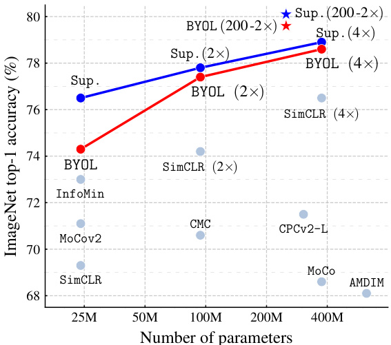
Figure 1: Performance of BYOL on ImageNet (linear evaluation) using ResNet-50 and our best architecture ResNet-200 $(2\times)$ , compared to other unsupervised and supervised (Sup.) baselines [8].
图 1: BYOL 在 ImageNet 上的性能 (线性评估) 使用 ResNet-50 和我们最佳架构 ResNet-200 $(2\times)$ ,与其他无监督和监督 (Sup.) 基线 [8] 的对比。
In this paper, we introduce Bootstrap Your Own Latent (BYOL), a new algorithm for self-supervised learning of image representations. BYOL achieves higher performance than state-of-the-art contrastive methods without using negative pairs. It iterative ly bootstraps 4 the outputs of a network to serve as targets for an enhanced representation. Moreover, BYOL is more robust to the choice of image augmentations than contrastive methods; we suspect that not relying on negative pairs is one of the leading reasons for its improved robustness. While previous methods based on boots trapping have used pseudo-labels [16], cluster indices [17] or a handful of labels [18, 19, 20], we propose to directly bootstrap the representations. In particular, BYOL uses two neural networks, referred to as online and target networks, that interact and learn from each other. Starting from an augmented view of an image, BYOL trains its online network to predict the target network’s representation of another augmented view of the same image. While this objective admits collapsed solutions, e.g., outputting the same vector for all images, we empirically show that BYOL does not converge to such solutions. We hypothesize (Section 3.2) that the combination of (i) the addition of a predictor to the online network and (ii) the use of a moving average of online parameters, as the target network encourages encoding more and more information in the online projection and avoids collapsed solutions.
本文介绍了一种新的图像表征自监督学习算法——自引导潜在空间(Bootstrap Your Own Latent,BYOL)。该算法在不使用负样本对的情况下,性能超越了当前最先进的对比学习方法。BYOL通过迭代式自引导网络输出来构建增强表征目标,且对图像增强策略的选择具有比对比学习更强的鲁棒性,我们认为这种优势主要源于其不依赖负样本对的特性。与以往基于自引导的方法[16]使用伪标签、[17]使用聚类索引或[18,19,20]使用少量标签不同,我们提出直接自引导表征本身。具体而言,BYOL采用在线网络和目标网络两个神经网络进行交互学习:从图像的增强视图出发,在线网络被训练用于预测同一图像另一增强视图在目标网络中的表征。虽然该目标函数存在坍缩解风险(例如对所有图像输出相同向量),但我们通过实验证明BYOL不会收敛到此类解。我们假设(第3.2节)这种特性源于:(i)在线网络预测器的引入,与(ii)采用在线参数移动平均值作为目标网络参数的双重机制,这种组合能促使在线投影编码更多信息并避免坍缩解。
We evaluate the representation learned by BYOL on ImageNet [21] and other vision benchmarks using ResNet architectures [22]. Under the linear evaluation protocol on ImageNet, consisting in training a linear classifier on top of the frozen representation, BYOL reaches $7\bar{4}.3%$ top-1 accuracy with a standard ResNet-50 and $79.6%$ top-1 accuracy with a larger ResNet (Figure 1). In the semi-supervised and transfer settings on ImageNet, we obtain results on par or superior to the current state of the art. Our contributions are: (i) We introduce BYOL, a self-supervised representation learning method (Section 3) which achieves state-of-the-art results under the linear evaluation protocol on ImageNet without using negative pairs. $(i i)$ We show that our learned representation outperforms the state of the art on semi-supervised and transfer benchmarks (Section 4). (iii) We show that BYOL is more resilient to changes in the batch size and in the set of image augmentations compared to its contrastive counterparts (Section 5). In particular, BYOL suffers a much smaller performance drop than SimCLR, a strong contrastive baseline, when only using random crops as image augmentations.
我们在ImageNet [21]和其他视觉基准测试中使用ResNet架构 [22]评估BYOL学习到的表示。在ImageNet的线性评估协议下(即在冻结表示之上训练线性分类器),BYOL使用标准ResNet-50达到74.3%的top-1准确率,使用更大的ResNet达到79.6%的top-1准确率(图1)。在ImageNet的半监督和迁移设置中,我们获得与当前最先进技术相当或更优的结果。我们的贡献包括:(i) 我们提出了BYOL(一种自监督表示学习方法)(第3节),该方法在ImageNet线性评估协议下不使用负样本对就达到了最先进的性能。(ii) 我们证明学习到的表示在半监督和迁移基准测试中优于现有技术(第4节)。(iii) 我们表明,与对比方法相比,BYOL对批次大小和图像增强集的变化更具适应性(第5节)。特别是当仅使用随机裁剪作为图像增强时,BYOL的性能下降远小于强对比基线SimCLR。
2 Related work
2 相关工作
Most unsupervised methods for representation learning can be categorized as either generative or disc rim i native [23, 8]. Generative approaches to representation learning build a distribution over data and latent embedding and use the learned embeddings as image representations. Many of these approaches rely either on auto-encoding of images [24, 25, 26] or on adversarial learning [27], jointly modelling data and representation [28, 29, 30, 31]. Generative methods typically operate directly in pixel space. This however is computationally expensive, and the high level of detail required for image generation may not be necessary for representation learning.
大多数无监督表示学习方法可分为生成式 (generative) 或判别式 (discriminative) [23, 8]。生成式表示学习方法构建数据和潜在嵌入的分布,并将学习到的嵌入作为图像表示。这些方法大多依赖于图像的自编码 (auto-encoding) [24, 25, 26] 或对抗学习 (adversarial learning) [27],同时对数据和表示进行联合建模 [28, 29, 30, 31]。生成式方法通常直接在像素空间操作,但计算成本较高,且图像生成所需的高细节水平对于表示学习可能并非必要。
Among disc rim i native methods, contrastive methods [9, 10, 32, 33, 34, 11, 35, 36] currently achieve state-of-the-art performance in self-supervised learning [37, 8, 38, 12]. Contrastive approaches avoid a costly generation step in pixel space by bringing representation of different views of the same image closer (‘positive pairs’), and spreading representations of views from different images (‘negative pairs’) apart [39, 40]. Contrastive methods often require comparing each example with many other examples to work well [9, 8] prompting the question of whether using negative pairs is necessary.
在判别式方法中,对比方法 [9, 10, 32, 33, 34, 11, 35, 36] 目前代表了自监督学习 [37, 8, 38, 12] 的最先进性能。对比方法通过拉近同一图像不同视角的表示("正样本对"),并推远不同图像视角的表示("负样本对")[39, 40],避免了像素空间中代价高昂的生成步骤。对比方法通常需要将每个样本与许多其他样本进行比较才能取得良好效果 [9, 8],这引发了是否需要使用负样本对的疑问。
Deep Cluster [17] partially answers this question. It uses boots trapping on previous versions of its representation to produce targets for the next representation; it clusters data points using the prior representation, and uses the cluster index of each sample as a classification target for the new representation. While avoiding the use of negative pairs, this requires a costly clustering phase and specific precautions to avoid collapsing to trivial solutions.
Deep Cluster [17] 部分回答了这个问题。它通过对先前表示版本进行自举 (bootstrapping) 来为下一个表示生成目标:使用先前的表示对数据点进行聚类,并将每个样本的聚类索引作为新表示的分类目标。虽然避免了使用负样本对,但这种方法需要昂贵的聚类阶段和特定的预防措施来避免坍缩到平凡解。
Some self-supervised methods are not contrastive but rely on using auxiliary handcrafted prediction tasks to learn their representation. In particular, relative patch prediction [23, 40], colorizing grayscale images [41, 42], image inpainting [43], image jigsaw puzzle [44], image super-resolution [45], and geometric transformations [46, 47] have been shown to be useful. Yet, even with suitable architectures [48], these methods are being outperformed by contrastive methods [37, 8, 12].
一些自监督方法并非对比式学习,而是依靠辅助手工设计的预测任务来学习表征。具体而言,相对块预测 [23, 40]、灰度图像着色 [41, 42]、图像修复 [43]、图像拼图 [44]、图像超分辨率 [45] 以及几何变换 [46, 47] 已被证明是有效的。然而,即使采用合适的架构 [48],这些方法的性能仍逊于对比式方法 [37, 8, 12]。
Our approach has some similarities with Predictions of Boots trapped Latents (PBL, [49]), a selfsupervised representation learning technique for reinforcement learning (RL). PBL jointly trains the agent’s history representation and an encoding of future observations. The observation encoding is used as a target to train the agent’s representation, and the agent’s representation as a target to train the observation encoding. Unlike PBL, BYOL uses a slow-moving average of its representation to provide its targets, and does not require a second network.
我们的方法与Predictions of Boots trapped Latents (PBL, [49])有相似之处,后者是一种用于强化学习(RL)的自监督表示学习技术。PBL同时训练智能体的历史表示和未来观测的编码,其中观测编码用作训练智能体表示的目标,而智能体表示则作为训练观测编码的目标。与PBL不同,BYOL使用其表示的缓慢移动平均值来提供目标,且不需要第二个网络。
The idea of using a slow-moving average target network to produce stable targets for the online network was inspired by deep RL [50, 51, 52, 53]. Target networks stabilize the boots trapping updates provided by the Bellman equation, making them appealing to stabilize the bootstrap mechanism in BYOL. While most RL methods use fixed target networks, BYOL uses a weighted moving average of previous networks (as in [54]) in order to provide smoother changes in the target representation.
使用缓慢移动的平均目标网络为在线网络生成稳定目标的想法源于深度强化学习 [50, 51, 52, 53]。目标网络稳定了由贝尔曼方程提供的自举更新,使其适用于稳定BYOL中的自举机制。虽然大多数强化学习方法使用固定目标网络,但BYOL采用了先前网络的加权移动平均 (如 [54] 所述) 以提供目标表征的更平滑变化。
In the semi-supervised setting [55, 56], an unsupervised loss is combined with a classification loss over a handful of labels to ground the training [19, 20, 57, 58, 59, 60, 61, 62]. Among these methods, mean teacher (MT) [20] also uses a slow-moving average network, called teacher, to produce targets for an online network, called student. An $\ell_{2}$ consistency loss between the softmax predictions of the teacher and the student is added to the classification loss. While [20] demonstrates the effectiveness of MT in the semi-supervised learning case, in Section 5 we show that a similar approach collapses when removing the classification loss. In contrast, BYOL introduces an additional predictor on top of the online network, which prevents collapse.
在半监督设定 [55, 56] 中,无监督损失与少量标签的分类损失相结合以稳定训练过程 [19, 20, 57, 58, 59, 60, 61, 62]。在这些方法中,均值教师 (MT) [20] 同样使用了一个缓慢更新的平均网络(称为教师网络)为在线网络(称为学生网络)生成目标。教师网络与学生网络的 softmax 预测之间的 $\ell_{2}$ 一致性损失被添加到分类损失中。虽然 [20] 证明了 MT 在半监督学习场景中的有效性,但我们在第 5 节表明,当移除分类损失时,类似方法会崩溃。相比之下,BYOL 在在线网络之上引入了一个额外的预测器,从而避免了崩溃。
Finally, in self-supervised learning, MoCo [9] uses a slow-moving average network (momentum encoder) to maintain consistent representations of negative pairs drawn from a memory bank. Instead, BYOL uses a moving average network to produce prediction targets as a means of stabilizing the bootstrap step. We show in Section 5 that this mere stabilizing effect can also improve existing contrastive methods.
最后,在自监督学习(self-supervised learning)中,MoCo [9] 使用了一个缓慢更新的平均网络(动量编码器)来保持从记忆库中提取的负样本对表示的一致性。而 BYOL 则采用移动平均网络来生成预测目标,以此稳定自举步骤。我们在第 5 节中表明,这种单纯的稳定效应同样可以改进现有的对比学习方法。
3 Method
3 方法
We start by motivating our method before explaining its details in Section 3.1. Many successful self-supervised learning approaches build upon the cross-view prediction framework introduced in [63]. Typically, these approaches learn representations by predicting different views (e.g., different random crops) of the same image from one another. Many such approaches cast the prediction problem directly in representation space: the representation of an augmented view of an image should be predictive of the representation of another augmented view of the same image. However, predicting directly in representation space can lead to collapsed representations: for instance, a representation that is constant across views is always fully predictive of itself. Contrastive methods circumvent this problem by reformulating the prediction problem into one of discrimination: from the representation of an augmented view, they learn to discriminate between the representation of another augmented view of the same image, and the representations of augmented views of different images. In the vast majority of cases, this prevents the training from finding collapsed representations. Yet, this disc rim i native approach typically requires comparing each representation of an augmented view with many negative examples, to find ones sufficiently close to make the discrimination task challenging. In this work, we thus tasked ourselves to find out whether these negative examples are indispensable to prevent collapsing while preserving high performance.
在详细解释方法之前(第3.1节),我们首先阐述研究动机。许多成功的自监督学习方法都基于[63]提出的跨视图预测框架。这类方法通常通过预测同一图像的不同视图(如不同随机裁剪区域)来学习表征。大多数方法直接在表征空间构建预测任务:图像增强视图的表征应能预测同一图像另一增强视图的表征。但直接在表征空间进行预测可能导致表征坍缩——例如,一个在所有视图中保持恒定的表征总能完美预测自身。对比学习方法通过将预测任务重构为判别任务来规避该问题:基于增强视图的表征,模型需要判别出属于同一图像的另一增强视图表征与不同图像的增强视图表征。这种方法在绝大多数情况下能避免训练得到坍缩表征。然而,这种判别式方法通常需要将每个增强视图的表征与大量负样本进行比较,以找到足够接近的样本来维持判别任务的挑战性。本研究旨在探究:在保持高性能的同时,这些负样本是否真是避免表征坍缩的必要条件。
To prevent collapse, a straightforward solution is to use a fixed randomly initialized network to produce the targets for our predictions. While avoiding collapse, it empirically does not result in very good representations. Nonetheless, it is interesting to note that the representation obtained using this procedure can already be much better than the initial fixed representation. In our ablation study (Section 5), we apply this procedure by predicting a fixed randomly initialized network and achieve $18.8%$ top-1 accuracy (Table 5a) on the linear evaluation protocol on ImageNet, whereas the randomly initialized network only achieves $1.4%$ by itself. This experimental finding is the core motivation for BYOL: from a given representation, referred to as target, we can train a new, potentially enhanced representation, referred to as online, by predicting the target representation. From there, we can expect to build a sequence of representations of increasing quality by iterating this procedure, using subsequent online networks as new target networks for further training. In practice, BYOL generalizes this boots trapping procedure by iterative ly refining its representation, but using a slowly moving exponential average of the online network as the target network instead of fixed checkpoints.
为防止训练崩溃,一个直接的解决方案是使用固定随机初始化的网络来生成预测目标。虽然这种方法避免了崩溃,但实验表明其产生的表征效果并不理想。不过值得注意的是,通过此方法获得的表征质量已显著优于初始固定表征。在我们的消融研究中(第5节),通过预测固定随机初始化网络,在ImageNet线性评估协议上达到了18.8%的top-1准确率(表5a),而随机初始化网络本身的准确率仅为1.4%。这一实验发现是BYOL的核心动机:从给定的目标表征出发,我们可以通过预测该目标表征来训练一个新的、可能增强的在线表征。由此,通过迭代这一过程(将后续在线网络作为新的目标网络继续训练),有望构建出质量逐步提升的表征序列。实际上,BYOL通过迭代优化其表征来推广这种自举过程,但采用在线网络的缓慢移动指数平均值作为目标网络,而非固定检查点。
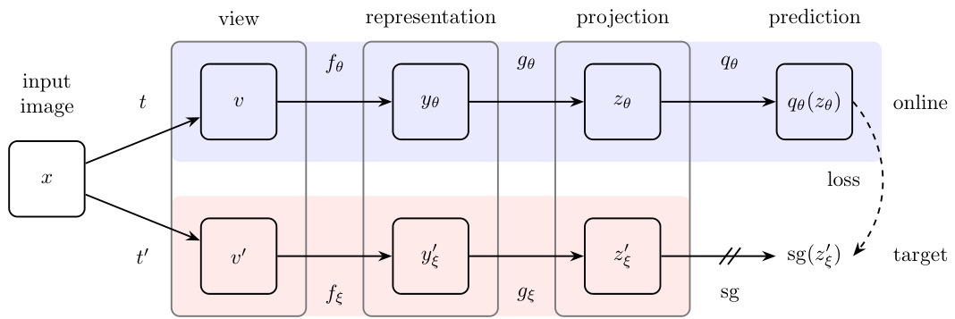
Figure 2: BYOL’s architecture. BYOL minimizes a similarity loss between $q_{\theta}(z_{\theta})$ and $\mathrm{sg}(z_{\xi}^{\prime})$ , where $\theta$ are the trained weights, $\xi$ are an exponential moving average of $\theta$ and sg means stop-gradient. At the end of training, everything but $f_{\theta}$ is discarded, and $y_{\theta}$ is used as the image representation.
图 2: BYOL架构示意图。BYOL通过最小化 $q_{\theta}(z_{\theta})$ 与 $\mathrm{sg}(z_{\xi}^{\prime})$ 之间的相似性损失进行训练,其中 $\theta$ 为可训练权重,$\xi$ 是 $\theta$ 的指数移动平均值,sg表示停止梯度。训练完成后仅保留 $f_{\theta}$ 模块,图像表征输出为 $y_{\theta}$。
3.1 Description of BYOL
3.1 BYOL描述
BYOL’s goal is to learn a representation $y_{\theta}$ which can then be used for downstream tasks. As described previously, BYOL uses two neural networks to learn: the online and target networks. The online network is defined by a set of weights $\theta$ and is comprised of three stages: an encoder $f_{\theta}$ , a projector $g_{\theta}$ and a predictor $q_{\theta}$ , as shown in Figure 2 and Figure 8. The target network has the same architecture as the online network, but uses a different set of weights $\xi$ . The target network provides the regression targets to train the online network, and its parameters $\xi$ are an exponential moving average of the online parameters $\theta$ [54]. More precisely, given a target decay rate $\tau\in[0,1]$ , after each training step we perform the following update,
BYOL的目标是学习一种可以用于下游任务的表示 $y_{\theta}$。如前所述,BYOL使用两个神经网络进行学习:在线网络和目标网络。在线网络由一组权重 $\theta$ 定义,包含三个阶段:编码器 $f_{\theta}$、投影器 $g_{\theta}$ 和预测器 $q_{\theta}$,如图2和图8所示。目标网络与在线网络结构相同,但使用另一组权重 $\xi$。目标网络提供回归目标来训练在线网络,其参数 $\xi$ 是在线参数 $\theta$ 的指数移动平均值 [54]。具体来说,给定目标衰减率 $\tau\in[0,1]$,在每次训练步骤后执行以下更新:
$$
\xi\leftarrow\tau\xi+(1-\tau)\theta.
$$
$$
\xi\leftarrow\tau\xi+(1-\tau)\theta.
$$
Given a set of images $\mathcal{D}$ , an image $x\sim\mathcal{D}$ sampled uniformly from $\mathcal{D}$ , and two distributions of image augmentations $\tau$ and $\mathcal{T}^{\prime}$ , BYOL produces two augmented views $v\triangleq t(x)$ and $v^{\prime}\triangleq t^{\prime}(x)$ from $x$ by applying respectively image augmentations $t\sim\tau$ and $t^{\prime}\sim\mathcal{T}^{\prime}$ . From the first augmented view $v$ , the online network outputs a representation $y_{\theta}\triangleq f_{\theta}(v)$ and a projection $z_{\theta}{\stackrel{\triangledown}{=}}g_{\theta}(y)$ . The target network outputs $y_{\xi}^{\prime}\triangleq f_{\xi}(v^{\prime})$ and the target projection $z_{\xi}^{\prime}\triangleq\bar{g}_ {\xi}(\bar{y}^{\prime})$ from the second augmented view $v^{\prime}$ . We then output a prediction $q_{\theta}(z_{\theta})$ of $z_{\xi}^{\prime}$ and $\ell_{2}$ -normalize both $q_{\theta}(z_{\theta})$ and $z_{\xi}^{\prime}$ to $\overline{{{q_{\theta}}}}(z_{\theta})\triangleq q_{\theta}(z_{\theta})/\lVert q_{\theta}(z_{\theta})\rVert_{2}$ and $\overline{{z}}_ {\xi}^{\prime}\triangleq z_{\xi}^{\prime}/\Vert z_{\xi}^{\prime}\Vert_{2}$ . Note that this predictor is only applied to the online branch, making the architecture asymmetric between the online and target pipeline. Finally we define the following mean squared error between the normalized predictions and target projections,5
给定一组图像 $\mathcal{D}$,从中均匀采样的图像 $x\sim\mathcal{D}$,以及两个图像增强分布 $\tau$ 和 $\mathcal{T}^{\prime}$,BYOL 通过分别应用图像增强 $t\sim\tau$ 和 $t^{\prime}\sim\mathcal{T}^{\prime}$ 从 $x$ 生成两个增强视图 $v\triangleq t(x)$ 和 $v^{\prime}\triangleq t^{\prime}(x)$。从第一个增强视图 $v$ 出发,在线网络输出一个表示 $y_{\theta}\triangleq f_{\theta}(v)$ 和一个投影 $z_{\theta}{\stackrel{\triangledown}{=}}g_{\theta}(y)$。目标网络从第二个增强视图 $v^{\prime}$ 输出 $y_{\xi}^{\prime}\triangleq f_{\xi}(v^{\prime})$ 和目标投影 $z_{\xi}^{\prime}\triangleq\bar{g}_ {\xi}(\bar{y}^{\prime})$。然后,我们输出 $z_{\xi}^{\prime}$ 的预测 $q_{\theta}(z_{\theta})$,并将 $q_{\theta}(z_{\theta})$ 和 $z_{\xi}^{\prime}$ 都进行 $\ell_{2}$ 归一化,得到 $\overline{{{q_{\theta}}}}(z_{\theta})\triangleq q_{\theta}(z_{\theta})/\lVert q_{\theta}(z_{\theta})\rVert_{2}$ 和 $\overline{{z}}_ {\xi}^{\prime}\triangleq z_{\xi}^{\prime}/\Vert z_{\xi}^{\prime}\Vert_{2}$。需要注意的是,这个预测器仅应用于在线分支,使得在线和目标流程之间的架构不对称。最后,我们定义了归一化预测和目标投影之间的均方误差,5
$$
\mathcal{L}_ {\theta,\xi}\triangleq\left\lVert\overline{{q_{\theta}}}(z_{\theta})-\overline{{z}}_ {\xi}^{\prime}\right\rVert_{2}^{2}=2-2\cdot\frac{\left\langle q_{\theta}(z_{\theta}),z_{\xi}^{\prime}\right\rangle}{\left\lVert q_{\theta}(z_{\theta})\right\rVert_{2}\cdot\left\lVert z_{\xi}^{\prime}\right\rVert_{2}}.
$$
$$
\mathcal{L}_ {\theta,\xi}\triangleq\left\lVert\overline{{q_{\theta}}}(z_{\theta})-\overline{{z}}_ {\xi}^{\prime}\right\rVert_{2}^{2}=2-2\cdot\frac{\left\langle q_{\theta}(z_{\theta}),z_{\xi}^{\prime}\right\rangle}{\left\lVert q_{\theta}(z_{\theta})\right\rVert_{2}\cdot\left\lVert z_{\xi}^{\prime}\right\rVert_{2}}.
$$
We symmetrize the loss $\mathcal{L}_ {\boldsymbol{\theta},\boldsymbol{\xi}}$ in Eq. 2 by separately feeding $v^{\prime}$ to the online network and $v$ to the target network to compute $\widetilde{\mathcal{L}}_ {\theta,\xi}$ . At each training step, we perform a stochastic optimization step to minimize BYOL $\mathcal{L}_ {\boldsymbol{\theta},\boldsymbol{\xi}}^{\mathtt{B Y O L}}=\mathcal{L}_ {\boldsymbol{\theta},\boldsymbol{\xi}}+\widetilde{\mathcal{L}}_{\boldsymbol{\theta},\boldsymbol{\xi}}$ with respect to $\theta$ only, but not $\xi$ , as depicted by the stop-gradient in Figure 2. BYOL’s dynamics eare summarized as
我们对等式2中的损失 $\mathcal{L}_ {\boldsymbol{\theta},\boldsymbol{\xi}}$ 进行对称化处理,分别将 $v^{\prime}$ 输入在线网络、$v$ 输入目标网络来计算 $\widetilde{\mathcal{L}}_ {\theta,\xi}$。在每个训练步骤中,我们执行随机优化步骤以最小化BYOL损失 $\mathcal{L}_ {\boldsymbol{\theta},\boldsymbol{\xi}}^{\mathtt{B Y O L}}=\mathcal{L}_ {\boldsymbol{\theta},\boldsymbol{\xi}}+\widetilde{\mathcal{L}}_{\boldsymbol{\theta},\boldsymbol{\xi}}$,但仅针对参数 $\theta$ 进行优化(不更新 $\xi$),如图2中的停止梯度所示。BYOL的动态机制可总结为

where optimizer is an optimizer and $\eta$ is a learning rate. At the end of training, we only keep the encoder $f_{\theta}$ ; as in [9]. When comparing to other methods, we consider the number of inference-time weights only in the final representation $f_{\theta}$ . The architecture, hyper-parameters and training details are specified in Appendix A, the full training procedure is summarized in Appendix B, and python pseudo-code based on the libraries JAX [64] and Haiku [65] is provided in in Appendix J.
其中 optimizer 是优化器,$\eta$ 是学习率。训练结束时,我们仅保留编码器 $f_{\theta}$;如 [9] 所述。在与其他方法比较时,我们仅考虑最终表示 $f_{\theta}$ 中的推理时权重数量。架构、超参数和训练细节详见附录 A,完整训练流程总结于附录 B,基于 JAX [64] 和 Haiku [65] 库的 Python语言 伪代码提供于附录 J。
3.2 Intuitions on BYOL’s behavior
3.2 关于BYOL行为的直观理解
minimizing $\mathcal{L}_{\boldsymbol{\theta},\boldsymbol{\xi}}^{\mathtt{B Y O L}}$ with respect to $\theta$ , it may seem that BYOL should converge to a minimum of this loss
最小化 $\mathcal{L}_{\boldsymbol{\theta},\boldsymbol{\xi}}^{\mathtt{B Y O L}}$ 关于 $\theta$ 时,看起来 BYOL 应该收敛到该损失的最小值
| Method | Top-1 | Top-5 |
| LocalAgg. | 60.2 | |
| PIRL[35] | 63.6 | |
| CPC v2[32] | 63.8 | 85.3 |
| CMC [11] | 66.2 | 87.0 |
| SimCLR [8] | 69.3 | 89.0 |
| MoCov2[37] | 71.1 | |
| InfoMinAug.[12] | 73.0 | 91.1 |
| BYOL (ours) | 74.3 | 91.6 |
(a) ResNet-50 encoder.
| 方法 | Top-1 | Top-5 |
|---|---|---|
| LocalAgg. | 60.2 | |
| PIRL[35] | 63.6 | |
| CPC v2[32] | 63.8 | 85.3 |
| CMC [11] | 66.2 | 87.0 |
| SimCLR [8] | 69.3 | 89.0 |
| MoCov2[37] | 71.1 | |
| InfoMinAug.[12] | 73.0 | 91.1 |
| BYOL (ours) | 74.3 | 91.6 |
(a) ResNet-50编码器。
| Method | Architecture | Param. | Top-1 | Top-5 |
| SimCLR[8] | ResNet-50(2×) | 94M | 74.2 | 92.0 |
| CMC [11] | ResNet-50(2x) | 94M | 70.6 | 89.7 |
| BYOL(ours) | ResNet-50 (2×) | 94M | 77.4 | 93.6 |
| CPC v2[32] | ResNet-161 | 305M | 71.5 | 90.1 |
| MoCo [9] | ResNet-50(4x) | 375M | 68.6 | |
| SimCLR[8] | ResNet-50 (4×) | 375M | 76.5 | 93.2 |
| BYOL (ours) | ResNet-50 (4×) | 375M | 78.6 | 94.2 |
| BYOL (ours) | ResNet-200 (2x) | 250M | 79.6 | 94.8 |
(b) Other ResNet encoder architectures.
| 方法 | 架构 | 参数量 | Top-1 | Top-5 |
|---|---|---|---|---|
| SimCLR[8] | ResNet-50(2×) | 94M | 74.2 | 92.0 |
| CMC [11] | ResNet-50(2×) | 94M | 70.6 | 89.7 |
| BYOL(ours) | ResNet-50 (2×) | 94M | 77.4 | 93.6 |
| CPC v2[32] | ResNet-161 | 305M | 71.5 | 90.1 |
| MoCo [9] | ResNet-50(4×) | 375M | 68.6 | |
| SimCLR[8] | ResNet-50 (4×) | 375M | 76.5 | 93.2 |
| BYOL (ours) | ResNet-50 (4×) | 375M | 78.6 | 94.2 |
| BYOL (ours) | ResNet-200 (2×) | 250M | 79.6 | 94.8 |
(b) 其他ResNet编码器架构。
Table 1: Top-1 and top-5 accuracies (in $%$ ) under linear evaluation on ImageNet.
表 1: ImageNet线性评估下的Top-1和Top-5准确率(以$%$计)。
with respect to $(\theta,\xi)$ (e.g., a collapsed constant representation). However BYOL’s target parameters $\xi$ updates are not in the direction of $\mathsf{\bar{V}}_ {\xi}\mathcal{L}_ {\theta,\xi}^{\mathtt{B Y O L}}$ . More generally, we hypothesize that there is no loss $L_{\theta,\xi}$ such that BYOL’s dynamics is a gradient descent on jointly over $\theta,\xi$ . This is similar to GANs [66], where there is no loss that is jointly minimized w.r.t. both the disc rim in at or and generator parameters. There is therefore no a priori reason why BYOL’s parameters would converge to a minimum of LBθ,YξO L. While BYOL’s dynamics still admit undesirable equilibria, we did not observe convergence to such equilibria in our experiments. In addition, when assuming BYOL’s predictor to be optimal6 i.e.,
关于 $(\theta,\xi)$ (例如坍塌的常量表示) 。然而BYOL的目标参数 $\xi$ 的更新方向并非 $\mathsf{\bar{V}}_ {\xi}\mathcal{L}_ {\theta,\xi}^{\mathtt{B Y O L}}$ 。更一般地,我们假设不存在损失函数 $L_{\theta,\xi}$ 能使BYOL的动力学过程成为 $\theta,\xi$ 上的联合梯度下降。这与GANs [66] 的情况类似——不存在能同时最小化判别器和生成器参数的损失函数。因此从先验角度而言,BYOL的参数没有必然收敛到LBθ,YξO L最小值的理由。虽然BYOL的动力学仍存在不理想的平衡点,但在实验中我们并未观察到收敛到此类平衡点的情况。此外,当假设BYOL的预测器处于最优状态6时,即
$$
q_{\theta}=q^{\star}\mathrm{with}q^{\star}\triangleq\operatorname*{argmin}_ {q}\mathbb{E}\Big[\big|q(z_{\theta})-z_{\xi}^{\prime}\big|_ {2}^{2}\Big],\quad\mathrm{where}\quad q^{\star}(z_{\theta})=\mathbb{E}\big[z_{\xi}^{\prime}|z_{\theta}\big],
$$
$$
q_{\theta}=q^{\star}\mathrm{with}q^{\star}\triangleq\operatorname*{argmin}_ {q}\mathbb{E}\Big[\big|q(z_{\theta})-z_{\xi}^{\prime}\big|_ {2}^{2}\Big],\quad\mathrm{where}\quad q^{\star}(z_{\theta})=\mathbb{E}\big[z_{\xi}^{\prime}|z_{\theta}\big],
$$
we hypothesize that the undesirable equilibria are unstable. Indeed, in this optimal predictor case, BYOL’s updates on $\theta$ follow in expectation the gradient of the expected conditional variance (see Appendix I for details), we note $z_{\xi,i}^{\bar{\prime}}$ the $i$ -th feature of $z_{\xi}^{\prime}$ , then
我们假设不良均衡是不稳定的。实际上,在这个最优预测器的情况下,BYOL对$\theta$的更新在期望上遵循预期条件方差的梯度(详见附录I),我们将$z_{\xi,i}^{\bar{\prime}}$记为$z_{\xi}^{\prime}$的第$i$个特征,那么
$$
\nabla_{\theta}\mathbb{E}\left[\left\Vert q^{\star}(z_{\theta})-z_{\xi}^{\prime}\right\Vert_{2}^{2}\right]=\nabla_{\theta}\mathbb{E}\left[\left\Vert\mathbb{E}\left[z_{\xi}^{\prime}|z_{\theta}\right]-z_{\xi}^{\prime}\right\Vert_{2}^{2}\right]=\nabla_{\theta}\mathbb{E}\left[\sum_{i}\mathrm{Var}(z_{\xi,i}^{\prime}|z_{\theta})\right],
$$
$$
\nabla_{\theta}\mathbb{E}\left[\left\Vert q^{\star}(z_{\theta})-z_{\xi}^{\prime}\right\Vert_{2}^{2}\right]=\nabla_{\theta}\mathbb{E}\left[\left\Vert\mathbb{E}\left[z_{\xi}^{\prime}|z_{\theta}\right]-z_{\xi}^{\prime}\right\Vert_{2}^{2}\right]=\nabla_{\theta}\mathbb{E}\left[\sum_{i}\mathrm{Var}(z_{\xi,i}^{\prime}|z_{\theta})\right],
$$
Note that for any random variables $X,Y,$ and $Z$ $\cdot,\operatorname{Var}(X|Y,Z)\leq\operatorname{Var}(X|Y)$ . Let $X$ be the target projection, $Y$ the current online projection, and $Z$ an additional variability on top of the online projection induced by stochastic i ties in the training dynamics: purely discarding information from the online projection cannot decrease the conditional variance.
注意,对于任意随机变量 $X,Y,$ 和 $Z$ ,有 $\cdot,\operatorname{Var}(X|Y,Z)\leq\operatorname{Var}(X|Y)$ 。设 $X$ 为目标投影, $Y$ 为当前在线投影, $Z$ 为训练动态中由随机性引入的在线投影上的额外变异性:纯粹丢弃在线投影的信息不会减少条件方差。
In particular, BYOL avoids constant features in $z_{\theta}$ as, for any constant $c$ and random variables $z_{\theta}$ and $z_{\xi}^{\prime}$ , $\mathrm{Var}(z_{\xi}^{\prime}|z_{\theta})\leq\mathrm{Var}(z_{\xi}^{\prime}|c)$ ; hence our hypothesis on these collapsed constant equilibria being unstable. Interestingly, if we were to minimize $\mathbb{E}[\sum_{i}\mathrm{Var}\big(z_{\xi,i}^{\prime}|z_{\theta}\big)]$ with respect to $\xi$ , we would get a collapsed $z_{\xi}^{\prime}$ as the variance is minimized for a constant $z_{\xi}^{\prime}$ . Instead, BYOL makes $\xi$ closer to $\theta$ , incorporating sources of variability captured by the online projection into the target projection.
具体而言,BYOL避免了 $z_{\theta}$ 中出现恒定特征,因为对于任意常数 $c$ 和随机变量 $z_{\theta}$ 与 $z_{\xi}^{\prime}$ ,有 $\mathrm{Var}(z_{\xi}^{\prime}|z_{\theta})\leq\mathrm{Var}(z_{\xi}^{\prime}|c)$ ;因此我们假设这些坍缩的恒定平衡点是不稳定的。有趣的是,如果我们针对 $\xi$ 最小化 $\mathbb{E}[\sum_{i}\mathrm{Var}\big(z_{\xi,i}^{\prime}|z_{\theta}\big)]$ ,就会得到一个坍缩的 $z_{\xi}^{\prime}$ ,因为当 $z_{\xi}^{\prime}$ 为常数时方差最小。相反,BYOL让 $\xi$ 更接近 $\theta$ ,将在线投影捕获的变异性来源整合到目标投影中。
Furthermore, notice that performing a hard-copy of the online parameters $\theta$ into the target parameters $\xi$ would be enough to propagate new sources of variability. However, sudden changes in the target network might break the assumption of an optimal predictor, in which case BYOL’s loss is not guaranteed to be close to the conditional variance. We hypothesize that the main role of BYOL’s moving-averaged target network is to ensure the near-optimality of the predictor over training; Section 5 and Appendix J provide some empirical support of this interpretation.
此外,注意到将在线参数 $\theta$ 硬拷贝到目标参数 $\xi$ 足以传播新的可变性来源。然而,目标网络的突然变化可能会打破最优预测器的假设,在这种情况下,BYOL 的损失不一定接近条件方差。我们假设 BYOL 的移动平均目标网络的主要作用是在训练过程中确保预测器的接近最优性;第 5 节和附录 J 为这一解释提供了一些实证支持。
6For simplicity we also consider BYOL without normalization (which performs reasonably close to BYOL, see Appendix G.6) nor sym me tri z ation.
| Method | Top-1 | Top-5 | ||
| 1% | 10% | 1% | 10% | |
| Supervised[77] | 25.4 | 56.4 | 48.4 | 80.4 |
| InstDisc | 39.2 | 77.4 | ||
| PIRL [35] | 57.2 | 83.8 | ||
| SimCLR[8] | 48.3 | 65.6 | 75.5 | 87.8 |
| BYOL(ours) | 53.2 | 68.8 | 78.4 | 89.0 |
(a) ResNet-50 encoder.
为简化起见,我们同样考虑不进行归一化(其表现与BYOL相当接近,参见附录G.6)和对称化的BYOL。
| 方法 | Top-1 | Top-5 | ||
|---|---|---|---|---|
| 1% | 10% | 1% | 10% | |
| Supervised[77] | 25.4 | 56.4 | 48.4 | 80.4 |
| InstDisc | 39.2 | 77.4 | ||
| PIRL [35] | 57.2 | 83.8 | ||
| SimCLR[8] | 48.3 | 65.6 | 75.5 | 87.8 |
| BYOL(ours) | 53.2 | 68.8 | 78.4 | 89.0 |
(a) ResNet-50编码器。
| Method | Architecture | Param. | Top-1 | Top-5 | ||
| 1% | 10% | 1% | 10% | |||
| CPCv2[32] | ResNet-161 | 305M | 77.9 | 91.2 | ||
| SimCLR [8] | ResNet-50(2×) | 94M | 58.5 | 71.7 | 83.0 | 91.2 |
| BYOL (ours) | ResNet-50(2×) | 94M | 62.2 | 73.5 | 84.1 | 91.7 |
| SimCLR [8] | ResNet-50(4x) | 375M | 63.0 | 74.4 | 85.8 | 92.6 |
| BYOL(ours) | ResNet-50(4x) | 375M | 69.1 | 75.7 | 87.9 | 92.5 |
| BYOL (ours) | ResNet-200 (2x) | 250M | 71.2 | 77.7 | 89.5 | 93.7 |
| 方法 | 架构 | 参数量 | Top-1 (1%) | Top-1 (10%) | Top-5 (1%) | Top-5 (10%) |
|---|---|---|---|---|---|---|
| CPCv2 [32] | ResNet-161 | 305M | - | - | 77.9 | 91.2 |
| SimCLR [8] | ResNet-50(2×) | 94M | 58.5 | 71.7 | 83.0 | 91.2 |
| BYOL (ours) | ResNet-50(2×) | 94M | 62.2 | 73.5 | 84.1 | 91.7 |
| SimCLR [8] | ResNet-50(4×) | 375M | 63.0 | 74.4 | 85.8 | 92.6 |
| BYOL (ours) | ResNet-50(4×) | 375M | 69.1 | 75.7 | 87.9 | 92.5 |
| BYOL (ours) | ResNet-200 (2×) | 250M | 71.2 | 77.7 | 89.5 | 93.7 |
(b) Other ResNet encoder architectures.
(b) 其他ResNet编码器架构。
Table 2: Semi-supervised training with a fraction of ImageNet labels.
表 2: 使用部分ImageNet标签的半监督训练
| Method | Food101 | CIFAR10 | CIFAR100 | Birdsnap | SUN397 | Cars | Aircraft | VOC2007 | DTD | Pets | Caltech-101 | Flowers |
| Linearevaluation: | ||||||||||||
| BYOL (ours) | 75.3 | 91.3 | 78.4 | 57.2 | 62.2 | 67.8 | 60.6 | 82.5 | 75.5 | 90.4 | 94.2 | 96.1 |
| SimCLR(repro) | 72.8 | 90.5 | 74.4 | 42.4 | 60.6 | 49.3 | 49.8 | 81.4 | 75.7 | 84.6 | 89.3 | 92.6 |
| SimCLR [8] | 68.4 | 90.6 | 71.6 | 37.4 | 58.8 | 50.3 | 50.3 | 80.5 | 74.5 | 83.6 | 90.3 | 91.2 |
| Supervised-IN [8] | 72.3 | 93.6 | 78.3 | 53.7 | 61.9 | 66.7 | 61.0 | 82.8 | 74.9 | 91.5 | 94.5 | 94.7 |
| Fine-tuned: | ||||||||||||
| BYOL (ours) | 88.5 | 97.8 | 86.1 | 76.3 | 63.7 | 91.6 | 88.1 | 85.4 | 76.2 | 91.7 | 93.8 | 97.0 |
| SimCLR (repro) | 87.5 | 97.4 | 85.3 | 75.0 | 63.9 | 91.4 | 87.6 | 84.5 | 75.4 | 89.4 | 91.7 | 96.6 |
| SimCLR [8] | 88.2 | 97.7 | 85.9 | 75.9 | 63.5 | 91.3 | 88.1 | 84.1 | 73.2 | 89.2 | 92.1 | 97.0 |
| Supervised-IN[8] | 88.3 | 97.5 | 86.4 | 75.8 | 64.3 | 92.1 | 86.0 | 85.0 | 74.6 | 92.1 | 93.3 | 97.6 |
| Random init[8] | 86.9 | 95.9 | 80.2 | 76.1 | 53.6 | 91.4 | 85.9 | 67.3 | 64.8 | 81.5 | 72.6 | 92.0 |
Table 3: Transfer learning results from ImageNet (IN) with the standard ResNet-50 architecture.
| 方法 | Food101 | CIFAR10 | CIFAR100 | Birdsnap | SUN397 | Cars | Aircraft | VOC2007 | DTD | Pets | Caltech-101 | Flowers |
|---|---|---|---|---|---|---|---|---|---|---|---|---|
| 线性评估: | ||||||||||||
| BYOL (ours) | 75.3 | 91.3 | 78.4 | 57.2 | 62.2 | 67.8 | 60.6 | 82.5 | 75.5 | 90.4 | 94.2 | 96.1 |
| SimCLR (复现) | 72.8 | 90.5 | 74.4 | 42.4 | 60.6 | 49.3 | 49.8 | 81.4 | 75.7 | 84.6 | 89.3 | 92.6 |
| SimCLR [8] | 68.4 | 90.6 | 71.6 | 37.4 | 58.8 | 50.3 | 50.3 | 80.5 | 74.5 | 83.6 | 90.3 | 91.2 |
| Supervised-IN [8] | 72.3 | 93.6 | 78.3 | 53.7 | 61.9 | 66.7 | 61.0 | 82.8 | 74.9 | 91.5 | 94.5 | 94.7 |
| 微调: | ||||||||||||
| BYOL (ours) | 88.5 | 97.8 | 86.1 | 76.3 | 63.7 | 91.6 | 88.1 | 85.4 | 76.2 | 91.7 | 93.8 | 97.0 |
| SimCLR (复现) | 87.5 | 97.4 | 85.3 | 75.0 | 63.9 | 91.4 | 87.6 | 84.5 | 75.4 | 89.4 | 91.7 | 96.6 |
| SimCLR [8] | 88.2 | 97.7 | 85.9 | 75.9 | 63.5 | 91.3 | 88.1 | 84.1 | 73.2 | 89.2 | 92.1 | 97.0 |
| Supervised-IN [8] | 88.3 | 97.5 | 86.4 | 75.8 | 64.3 | 92.1 | 86.0 | 85.0 | 74.6 | 92.1 | 93.3 | 97.6 |
| Random init [8] | 86.9 | 95.9 | 80.2 | 76.1 | 53.6 | 91.4 | 85.9 | 67.3 | 64.8 | 81.5 | 72.6 | 92.0 |
表 3: 使用标准 ResNet-50 架构从 ImageNet (IN) 迁移学习的结果。
4 Experimental evaluation
4 实验评估
We assess the performance of BYOL’s representation after self-supervised pre training on the training set of the ImageNet ILSVRC-2012 dataset [21]. We first evaluate it on ImageNet (IN) in both linear evaluation and semi-supervised setups. We then measure its transfer capabilities on other datasets and tasks, including classification, segmentation, object detection and depth estimation. For comparison, we also report scores for a representation trained using labels from the train ImageNet subset, referred to as Supervised-IN. In Appendix F, we assess the generality of BYOL by pre training a representation on the Places365-Standard dataset [73] before reproducing this evaluation protocol.
我们在ImageNet ILSVRC-2012数据集[21]的训练集上通过自监督预训练评估BYOL的表征性能。首先在ImageNet (IN)上以线性评估和半监督设置进行测试,随后在其他数据集和任务(包括分类、分割、目标检测和深度估计)上衡量其迁移能力。作为对比,我们还报告了使用ImageNet训练子集标签训练的监督式IN表征得分。附录F中,我们通过在Places365-Standard数据集[73]上预训练表征并复现本评估方案,验证BYOL的泛化性。
Linear evaluation on ImageNet We first evaluate BYOL’s representation by training a linear classifier on top of the frozen representation, following the procedure described in [48, 74, 41, 10, 8], and appendix D.1; we report top-1 and top-5 accuracies in $%$ on the test set in Table 1. With a standard ResNet-50 $(\times1)$ BYOL obtains $74.3%$ top-1 accuracy $(91.6%$ top-5 accuracy), which is a $1.3%$ (resp. $0.5%$ ) improvement over the previous self-supervised state of the art [12]. This tightens the gap with respect to the supervised baseline of [8], $\bar{7}6.5%$ , but is still significantly below the stronger supervised baseline of [75], $78.9%$ . With deeper and wider architectures, BYOL consistently outperforms the previous state of the art (Appendix D.2), and obtains a best performance of $79.6%$ top-1 accuracy, ranking higher than previous self-supervised approaches. On a ResNet-50 $(4\times)$ BYOL achieves $78.6%$ , similar to the $78.9%$ of the best supervised baseline in [8] for the same architecture.
ImageNet上的线性评估
我们首先按照[48, 74, 41, 10, 8]和附录D.1描述的方法,通过在冻结表示上训练线性分类器来评估BYOL的表征性能。测试集的top-1和top-5准确率(单位:%)如 表1 所示。使用标准ResNet-50 $(\times1)$ 时,BYOL取得了 $74.3%$ 的top-1准确率 $(91.6%$ top-5准确率),相比之前最先进的自监督方法[12]提升了 $1.3%$ (对应 $0.5%$ )。这缩小了与监督基线[8] $\bar{7}6.5%$ 的差距,但仍显著低于更强监督基线[75]的 $78.9%$ 。采用更深更宽架构时,BYOL持续超越先前最优水平(附录D.2),并以 $79.6%$ 的top-1准确率创下新高,排名超过以往所有自监督方法。在ResNet-50 $(4\times)$ 架构上,BYOL达到 $78.6%$ ,与同架构下[8]最佳监督基线的 $78.9%$ 相当。
Semi-supervised training on ImageNet Next, we evaluate the performance obtained when finetuning BYOL’s representation on a classification task with a small subset of ImageNet’s train set, this time using label information. We follow the semi-supervised protocol of [74, 76, 8, 32] detailed in Appendix D.1, and use the same fixed splits of respectively $\bar{1}%$ and $10%$ of ImageNet labeled training data as in [8]. We report both top-1 and top-5 accuracies on the test set in Table 2. BYOL consistently outperforms previous approaches across a wide range of architectures. Additionally, as detailed in Appendix D.1, BYOL reaches $77.7%$ top-1 accuracy with ResNet-50 when fine-tuning over $100%$ of ImageNet labels.
ImageNet上的半监督训练
接下来,我们评估BYOL在小规模ImageNet训练集子集上进行分类任务微调时的表现,这次使用了标签信息。我们遵循[74, 76, 8, 32]中详述的半监督协议(见附录D.1),并采用与[8]相同的固定划分方式(分别使用$\bar{1}%$和$10%$的ImageNet标注训练数据)。表2展示了测试集的top-1和top-5准确率。BYOL在不同架构上始终优于先前方法。此外,如附录D.1所述,当使用ResNet-50对100% ImageNet标签进行微调时,BYOL达到了77.7%的top-1准确率。
Transfer to other classification tasks We evaluate our representation on other classification datasets to assess whether the features learned on ImageNet (IN) are generic and thus useful across image domains, or if they are ImageNet-specific. We perform linear evaluation and fine-tuning on the same set of classification tasks used in [8, 74], and carefully follow their evaluation protocol, as detailed in Appendix E. Performance is reported using standard metrics for each benchmark, and results are provided on a held-out test set after hyper parameter selection on a validation set. We report results in Table 3, both for linear evaluation and fine-tuning. BYOL outperforms SimCLR on all benchmarks and the Supervised-IN baseline on 7 of the 12 benchmarks, providing only slightly worse performance on the 5 remaining benchmarks. BYOL’s representation can transfer to small images, e.g., CIFAR [78], landscapes, e.g., SUN397 [79] or VOC2007 [80], and textures, e.g., DTD [81].
迁移到其他分类任务
我们在其他分类数据集上评估所学习的表征,以判断这些在ImageNet (IN) 上学到的特征是通用的(因而能跨图像领域适用),还是仅针对ImageNet的。我们采用[8, 74]中相同的分类任务集进行线性评估和微调,并严格遵循其评估协议(详见附录E)。性能报告使用各基准的标准指标,超参数通过验证集选择后在独立测试集上给出结果。表3展示了线性评估和微调的对比结果:BYOL在所有基准上都优于SimCLR,并在12个基准中的7个上超越了Supervised-IN基线,仅在剩余5个基准上表现略逊。BYOL的表征可迁移至小图像(如CIFAR [78])、自然场景(如SUN397 [79]或VOC2007 [80])以及纹理(如DTD [81])。
Transfer to other vision tasks We evaluate our representation on different tasks relevant to computer vision practitioners, namely semantic segmentation, object detection and depth estimation. With this evaluation, we assess whether BYOL’s representation generalizes beyond classification tasks.
迁移至其他视觉任务
我们评估了我们的表征在与计算机视觉从业者相关的不同任务上的表现,即语义分割、目标检测和深度估计。通过这一评估,我们验证了BYOL的表征是否能够泛化至分类任务之外。
We first evaluate BYOL on the VOC2012 semantic segmentation task as detailed in Appendix E.4, where the goal is to classify each pixel in the image [7]. We report the results in Table 4a. BYOL outperforms both the Supervised-IN baseline $+1.9$ mIoU) and SimCLR ( $+1.1$ mIoU).
我们首先在VOC2012语义分割任务上评估BYOL (详见附录E.4) ,该任务的目标是对图像中的每个像素进行分类 [7] 。结果如表4a所示,BYOL的表现优于监督式ImageNet基线 (提升1.9 mIoU) 和SimCLR (提升1.1 mIoU) 。
Similarly, we evaluate on object detection by reproducing the setup in [9] using a Faster R-CNN architecture [82], as detailed in Appendix E.5. We fine-tune on train val 2007 and report results on test2007 using the standard $\mathrm{AP_{50}}$ metric; BYOL is significantly better than the SupervisedIN baseline $(+3.1\mathrm{AP}_ {50})$ ) and SimCLR $(+2.3\mathrm{AP}_{50}) $ ).
同样地,我们通过使用Faster R-CNN架构[82]复现[9]中的设置来评估目标检测性能,具体细节见附录E.5。我们在trainval2007上微调,并使用标准$\mathrm{AP_{50}}$指标在test2007上报告结果;BYOL显著优于SupervisedIN基线$(+3.1\mathrm{AP}_ {50})$)和SimCLR$(+2.3\mathrm{AP}_{50})$)。
Finally, we evaluate on depth estimation on the NYU v2 dataset, where the depth map of a scene is estimated given a single RGB image. Depth prediction measures how well a network represents geometry, and how well that information can be localized to pixel accuracy [40]. The setup is based on [83] and detailed in Appendix E.6. We evaluate on the commonly used test subset of 654 images and report results using several common metrics in Table 4b: relative (rel) error, root mean squared (rms) error, and the percent of pixels (pct) where the error, $\operatorname*{max}(d_{g t}/d_{p},d_{p}/d_{g t})$ , is below $1.25^{n}$ thresholds where $d_{p}$ is the predicted depth and $d_{g t}$ is the ground truth depth [40]. BYOL is better or on par with other methods for each metric. For instance, the challenging pct. $<1.25$ measure is respectively improved by $+3.5$ points and $+1.3$ points compared to supervised and SimCLR baselines.
最后,我们在 NYU v2 数据集上进行深度估计评估,即给定单张 RGB 图像预测场景的深度图。深度预测衡量了网络对几何结构的表征能力,以及该信息能否精确定位到像素级 [40]。实验设置基于 [83],具体细节见附录 E.6。我们在常用的 654 张测试子集上评估,并使用表 4b 中的多个常用指标报告结果:相对 (rel) 误差、均方根 (rms) 误差,以及误差 $\operatorname*{max}(d_{g t}/d_{p},d_{p}/d_{g t})$ 低于 $1.25^{n}$ 阈值的像素百分比 (pct),其中 $d_{p}$ 为预测深度,$d_{g t}$ 为真实深度 [40]。BYOL 在各项指标上均优于或持平其他方法。例如,具有挑战性的 pct. $<1.25$ 指标相比监督学习和 SimCLR 基线分别提升了 $+3.5$ 和 $+1.3$ 个百分点。
| Method | AP50 | mloU | Lowerbetter | ||||||
| Supervised-IN [9] | 74.4 | 74.4 | Method | pct.<1.25 | pct.<1.252 | pct.<1.253 | rms | rel | |
| MoCo[9] | 74.9 | 72.5 | Supervised-IN [83] | 81.1 | 95.3 | 98.8 | 0.573 | 0.127 | |
| SimCLR (repro) | 75.2 | 75.2 | SimCLR (repro) | 83.3 | 96.5 | 99.1 | 0.557 | 0.134 | |
| BYOL (ours) | 77.5 | 76.3 | BYOL(ours) | 84.6 | 96.7 | 99.1 | 0.541 | 0.129 | |
(b) Transfer results on NYU v2 depth estimation.
| 方法 | AP50 | mloU | 方法 | pct.<1.25 | pct.<1.252 | pct.<1.253 | rms | rel |
|---|---|---|---|---|---|---|---|---|
| Supervised-IN [9] | 74.4 | 74.4 | Supervised-IN [83] | 81.1 | 95.3 | 98.8 | 0.573 | 0.127 |
| MoCo[9] | 74.9 | 72.5 | SimCLR (repro) | 83.3 | 96.5 | 99.1 | 0.557 | 0.134 |
| SimCLR (repro) | 75.2 | 75.2 | BYOL(ours) | 84.6 | 96.7 | 99.1 | 0.541 | 0.129 |
| BYOL (ours) | 77.5 | 76.3 |
(b) NYU v2深度估计迁移结果。
(a) Transfer results in semantic segmentation and object detection.
(a) 语义分割和目标检测中的迁移结果
Table 4: Results on transferring BYOL’s representation to other vision tasks.
表 4: BYOL表征迁移到其他视觉任务的结果
5 Building intuitions with ablations
5 通过消融实验建立直觉
We present ablations on BYOL to give an intuition of its behavior and performance. For reproducibility, we run each configuration of parameters over three seeds, and report the average performance. We also report the half difference between the best and worst runs when it is larger than 0.25. Although previous works perform ablations at 100 epochs [8, 12], we notice that relative improvements at 100 epochs do not always hold over longer training. For this reason, we run ablations over 300 epochs on 64 TPU v3 cores, which yields consistent results compared to our baseline training of 1000 epochs. For all the experiments in this section, we set the initial learning rate to 0.3 with batch size 4096, the weight decay to $10^{-6}$ as in SimCLR [8] and the base target decay rate $\tau_{\mathrm{base}}$ to 0.99. In this section we report results in top-1 accuracy on ImageNet under the linear evaluation protocol as in Appendix D.1.
我们对BYOL进行消融实验,以直观理解其行为和性能。为确保可复现性,每种参数配置均运行三次随机种子,并报告平均性能。当最佳与最差运行结果差异超过0.25时,我们会额外报告半差值。尽管先前研究多在100轮次进行消融实验[8,12],但我们发现100轮次的相对改进在更长训练周期中未必持续有效。因此,我们在64个TPU v3核心上进行了300轮次的消融实验,其结果与1000轮次基线训练具有一致性。本节所有实验均设置初始学习率为0.3(批量大小4096),权重衰减为$10^{-6}$(与SimCLR[8]一致),基础目标衰减率$\tau_{\mathrm{base}}$为0.99。本节结果采用ImageNet线性评估协议下的top-1准确率(详见附录D.1)。
Batch size Among contrastive methods, the ones that draw negative examples from the minibatch suffer performance drops when their batch size is reduced. BYOL does not use negative examples and we expect it to be more robust to smaller batch sizes. To empirically verify this hypothesis, we train both BYOL and SimCLR using different batch sizes from 128 to 4096. To avoid re-tuning other hyper parameters, we average gradients over $N$ consecutive steps before updating the online network when reducing the batch size by a factor $N$ . The target network is updated once every $N$ steps, after the update of the online network; we accumulate the $N$ -steps in parallel in our runs. As shown in Figure 3a, the performance of SimCLR rapidly deteriorates with batch size, likely due to the decrease in the number of negative examples. In contrast, the performance of BYOL remains stable over a wide range of batch sizes from 256 to 4096, and only drops for smaller values due to batch normalization layers in the encoder.7
批量大小
在对比方法中,那些从小批量(minibatch)中抽取负样本的方法在批量减小时性能会下降。BYOL不使用负样本,因此我们预期它对较小批量更具鲁棒性。为验证这一假设,我们使用128至4096的不同批量大小分别训练BYOL和SimCLR。为避免重新调整其他超参数,当批量缩小N倍时,我们会在更新在线网络前对连续N步的梯度取平均。目标网络每N步更新一次(在线网络更新后进行),实验中我们并行累积N步。如图3a所示,SimCLR性能随批量减小而快速恶化,这可能是由于负样本数量减少所致。相比之下,BYOL在256至4096的广泛批量范围内保持稳定性能,仅在更小批量时因编码器中的批量归一化层而出现下降[7]。
Image augmentations Contrastive methods are sensitive to the choice of image augmentations. For instance, SimCLR does not work well when removing color distortion from its image augmentations. As an explanation, $\mathtt{S i m C L R}$ shows that crops of the same image mostly share their color histograms. At the same time, color histograms vary across images. Therefore, when a contrastive task only relies on random crops as image augmentations, it can be mostly solved by focusing on color histograms alone. As a result the representation is not in centi viz ed to retain information beyond color histograms. To prevent that, SimCLR adds color distortion to its set of image augmentations. Instead, BYOL is in centi viz ed to keep any information captured by the target representation into its online network, to improve its predictions. Therefore, even if augmented views of a same image share the same color histogram, BYOL is still in centi viz ed to retain additional features in its representation. For that reason, we believe that BYOL is more robust to the choice of image augmentations than contrastive methods.
图像增强
对比方法对图像增强的选择非常敏感。例如,当从图像增强中移除颜色失真时,SimCLR表现不佳。对此,$\mathtt{SimCLR}$指出,同一图像的裁剪区域通常共享相同的颜色直方图,而不同图像之间的颜色直方图则存在差异。因此,当对比任务仅依赖随机裁剪作为图像增强时,仅通过关注颜色直方图就能基本解决该任务,导致表征无法集中保留颜色直方图之外的信息。为防止这一问题,SimCLR在其图像增强集中添加了颜色失真。
相比之下,BYOL的目标是将目标表征捕获的任何信息保留到其在线网络中,以改进预测。因此,即使同一图像的不同增强视图共享相同的颜色直方图,BYOL仍会集中保留表征中的其他特征。基于此,我们认为BYOL对图像增强的选择比对比方法更具鲁棒性。

Figure 3: Decrease in top-1 accuracy (in $%$ points) of BYOL and our own reproduction of SimCLR at 300 epochs, under linear evaluation on ImageNet.
图 3: BYOL 和我们自行复现的 SimCLR 在 ImageNet 线性评估下,经过 300 轮训练后 top-1 准确率 (以 $%$ 为单位) 的下降情况。
Results presented in Figure 3b support this hypothesis: the performance of BYOL is much less affected than the performance of SimCLR when removing color distortions from the set of image augmentations ( $-9.1$ accuracy points for BYOL, $-22.2$ accuracy points for SimCLR). When image augmentations are reduced to mere random crops, BYOL still displays good performance $(59.4%$ , i.e. $-13.1$ points from $72.5%$ ), while SimCLR loses more than a third of its performance ( $40.3%$ , i.e. $-27.6$ points from $67.9%$ ). We report additional ablations in Appendix G.3.
图 3b 展示的结果支持这一假设:当从图像增强组合中去除色彩失真时,BYOL的性能受影响程度远小于SimCLR (BYOL下降9.1个准确点,SimCLR下降22.2个准确点)。当图像增强仅保留随机裁剪时,BYOL仍保持良好性能 (59.4%,即从72.5%下降13.1个点),而SimCLR性能损失超过三分之一 (40.3%,即从67.9%下降27.6个点)。更多消融实验结果详见附录G.3。
Boots trapping BYOL uses the projected representation of a target network, whose weights are an exponential moving average of the weights of the online network, as target for its predictions. This way, the weights of the target network represent a delayed and more stable version of the weights of the online network. When the target decay rate is 1, the target network is never updated, and remains at a constant value corresponding to its initialization. When the target decay rate is 0, the target network is instantaneously updated to the online network at each step. There is a trade-off between updating the targets too often and updating them too slowly, as illustrated in Table 5a. Instantaneously updating the target network $\mathrm{\Delta}_{T}=0\mathrm{\Delta}$ ) destabilize s training, yielding very poor performance while never updating the target $(\tau=1)$ ) makes the training stable but prevents iterative improvement, ending with low-quality final representation. All values of the decay rate between 0.9 and 0.999 yield performance above $68.{\dot{4}}%$ top-1 accuracy at 300 epochs.
BYOL的自举策略使用目标网络的投影表示作为预测目标,该目标网络的权重是在线网络权重的指数移动平均值。这种方式使得目标网络的权重成为在线网络权重的延迟且更稳定的版本。当目标衰减率为1时,目标网络永不更新,保持初始化的恒定值;当目标衰减率为0时,目标网络会在每一步立即更新为在线网络。如表5a所示,目标更新频率存在权衡:立即更新目标网络($\mathrm{\Delta}_{T}=0\mathrm{\Delta}$)会导致训练失稳,性能极差;而永不更新目标($\tau=1$)虽能稳定训练,但会阻碍迭代优化,最终得到低质量表征。衰减率在0.9至0.999之间时,300轮训练后的top-1准确率均能超过$68.{\dot{4}}%$。
Table 5: Ablations with top-1 accuracy (in $%$ ) at 300 epochs under linear evaluation on ImageNet.
| Target | Tbase | Top-1 |
| Constantrandomnetwork | 1 | 18.8±0.7 |
| Moving average of online | 0.999 | 69.8 |
| Movinga averageofonline | 0.99 | 72.5 |
| Moving average of online | 0.9 | 68.4 |
| Stopgradient of online | 0 | 0.3 |
(a) Results for different target modes. †In the stop gradient of online, $\tau=\tau_{\mathrm{base}}=0$ is kept constant throughout training.
表 5: 在ImageNet线性评估下300个epoch时的Top-1准确率(单位: $%$ )消融实验。
| 目标 | Tbase | Top-1 |
|---|---|---|
| 恒定随机网络 | 1 | 18.8±0.7 |
| 在线移动平均 | 0.999 | 69.8 |
| 在线移动平均 | 0.99 | 72.5 |
| 在线移动平均 | 0.9 | 68.4 |
| 在线停止梯度 | 0 | 0.3 |
(a) 不同目标模式的结果。†在在线停止梯度中, $\tau=\tau_{\mathrm{base}}=0$ 在整个训练过程中保持恒定。
(b) Intermediate variants between BYOL and SimCLR.
| 方法 | 预测器 | 目标网络 | B | Top-1 |
|---|---|---|---|---|
| BYOL | √ | √ | 0 | 72.5 |
| — | √ | √ | 1 | 70.9 |
| — | √ | 1 | 70.7 | |
| SimCLR | 1 | 69.4 | ||
| — | √ | 1 | 69.1 | |
| — | √ | 0 | 0.3 | |
| √ | 0 | 0.2 | ||
| — | 0 | 0.1 |
(b) BYOL与SimCLR之间的中间变体。
Ablation to contrastive methods In this subsection, we recast SimCLR and BYOL using the same formalism to better understand where the improvement of BYOL over SimCLR comes from. Let us consider the following objective that extends the InfoNCE objective [10, 84] (see Appendix G.4),
对比方法的消融研究
在本小节中,我们采用相同形式化方法重构SimCLR和BYOL,以更深入理解BYOL相对于SimCLR的改进来源。考虑以下扩展InfoNCE目标函数[10,84]的目标(详见附录G.4),
$$
\mathrm{InfoNCE}_ {\theta}^{\alpha,\beta}\triangleq\frac{2}{B}\sum_{i=1}^{B}S_{\theta}(v_{i},v_{i}^{\prime})-\beta\cdot\frac{2\alpha}{B}\sum_{i=1}^{B}\ln\left(\sum_{j\neq i}\exp\frac{S_{\theta}(v_{i},v_{j})}{\alpha}+\sum_{j}\exp\frac{S_{\theta}(v_{i},v_{j}^{\prime})}{\alpha}\right),
$$
$$
\mathrm{InfoNCE}_ {\theta}^{\alpha,\beta}\triangleq\frac{2}{B}\sum_{i=1}^{B}S_{\theta}(v_{i},v_{i}^{\prime})-\beta\cdot\frac{2\alpha}{B}\sum_{i=1}^{B}\ln\left(\sum_{j\neq i}\exp\frac{S_{\theta}(v_{i},v_{j})}{\alpha}+\sum_{j}\exp\frac{S_{\theta}(v_{i},v_{j}^{\prime})}{\alpha}\right),
$$
where $\alpha>0$ is a fixed temperature, $\beta\in[0,1]$ a weighting coefficient, $B$ the batch size, $v$ and $v^{\prime}$ are batches of augmented views where for any batch index $i$ , $v_{i}$ and $\boldsymbol{v}{i}^{\prime}$ are augmented views from the same image; the real-valued function $S{\theta}$ quantifies pairwise similarity between augmented views. For any augmented view $u$ we denote $z_{\theta}(u)\triangleq f_{\theta}(g_{\theta}(u))$ and $z_{\xi}(u)\triangleq f_{\xi}(g_{\xi}(u))$ . For given $\phi$ and $\psi$ , we consider the normalized dot product
其中 $\alpha>0$ 是固定温度参数,$\beta\in[0,1]$ 为权重系数,$B$ 表示批处理大小,$v$ 和 $v^{\prime}$ 是增强视图批次,对于任意批次索引 $i$,$v_{i}$ 和 $\boldsymbol{v}{i}^{\prime}$ 来自同一图像的增强视图;实值函数 $S{\theta}$ 用于量化增强视图间的成对相似度。对于任意增强视图 $u$,我们记 $z_{\theta}(u)\triangleq f_{\theta}(g_{\theta}(u))$ 和 $z_{\xi}(u)\triangleq f_{\xi}(g_{\xi}(u))$。给定 $\phi$ 和 $\psi$ 时,我们考虑归一化点积
$$
S_{\theta}(u_{1},u_{2})\triangleq\frac{\langle\phi(u_{1}),\psi(u_{2})\rangle}{|\phi(u_{1})|_ {2}\cdot|\psi(u_{2})|_{2}}.
$$
$$
S_{\theta}(u_{1},u_{2})\triangleq\frac{\langle\phi(u_{1}),\psi(u_{2})\rangle}{|\phi(u_{1})|_ {2}\cdot|\psi(u_{2})|_{2}}.
$$
Up to minor details (cf. Appendix G.5), we recover the SimCLR loss with $\phi(u_{1}):=:z_{\theta}(u_{1})$ (no predictor), $\psi(u_{2})=z_{\theta}(u_{2})$ (no target network) and $\beta=1$ . We recover the BYOL loss when using a predictor and a target network, i.e., $\phi(u_{1})=p_{\theta}(z_{\theta}(u_{1}))$ and $\psi(u_{2})=z_{\xi}(u_{2})$ with $\beta=0$ . To evaluate the influence of the target network, the predictor and the coefficient $\beta$ , we perform an ablation over them. Results are presented in Table 5b and more details are given in Appendix G.4. The only variant that performs well without negative examples (i.e., with $\beta=0$ ) is BYOL, using both a bootstrap target network and a predictor. Adding the negative pairs to BYOL’s loss without re-tuning the temperature parameter hurts its performance. In Appendix G.4, we show that we can add back negative pairs and still match the performance of BYOL with proper tuning of the temperature.
除细微差异外(参见附录 G.5),当设置$\phi(u_{1}):=:z_{\theta}(u_{1})$(无预测头)、$\psi(u_{2})=z_{\theta}(u_{2})$(无目标网络)且$\beta=1$时,我们还原了SimCLR损失函数。当使用预测头和目标网络时(即$\phi(u_{1})=p_{\theta}(z_{\theta}(u_{1}))$和$\psi(u_{2})=z_{\xi}(u_{2})$且$\beta=0$),我们还原了BYOL损失函数。为评估目标网络、预测头及系数$\beta$的影响,我们对其进行了消融实验。结果如 表 5b 所示,更多细节见附录 G.4。唯一能在不使用负样本(即$\beta=0$)情况下表现良好的变体是同时采用目标网络和预测头的BYOL。若在BYOL损失函数中直接添加负样本对而不重新调整温度参数,会损害其性能。附录 G.4 表明,通过适当调整温度参数,我们可以在保留负样本对的情况下仍达到BYOL的性能水平。
Simply adding a target network to $\mathtt{S i m C L R}$ already improves performance $(+1.6\$ points). This sheds new light on the use of the target network in MoCo [9], where the target network is used to provide more negative examples. Here, we show that by mere stabilization effect, even when using the same number of negative examples, using a target network is beneficial. Finally, we observe that modifying the architecture of $S_{\theta}$ to include a predictor only mildly affects the performance of $\mathtt{S i m C L R}$ .
仅向 $\mathtt{SimCLR}$ 添加目标网络即可提升性能 $(+1.6$ 分) 。这一发现为MoCo [9] 中目标网络的作用提供了新视角 (原用于提供更多负样本) 。我们证明仅通过稳定效应,即使使用相同数量的负样本,目标网络仍能带来收益。最后,我们观察到修改 $S_{\theta}$ 架构以包含预测器对 $\mathtt{SimCLR}$ 性能影响较小。
Relationship with Mean Teacher Another semi-supervised approach, Mean Teacher (MT) [20], complements a supervised loss on few labels with an additional consistency loss. In [20], this consistency loss is the $\ell_{2}$ distance between the logits from a student network, and those of a temporally averaged version of the student network, called teacher. Removing the predictor in BYOL results in an unsupervised version of MT with no classification loss that uses image augmentations instead of the original architectural noise (e.g., dropout). This variant of BYOL collapses (Row 7 of ??) which suggests that the additional predictor is critical to prevent collapse in an unsupervised scenario.
与Mean Teacher的关系
另一种半监督方法Mean Teacher (MT) [20]通过额外的一致性损失补充了少标签监督损失。在[20]中,该一致性损失是学生网络的logits与称为教师网络的学生网络时间平均版本logits之间的$\ell_{2}$距离。BYOL中移除预测器会得到一个无监督版本的MT,该版本不使用分类损失,而是用图像增强替代原始架构噪声(如dropout)。BYOL的这种变体会崩溃(见??第7行),这表明额外的预测器对于防止无监督场景中的崩溃至关重要。
Importance of a near-optimal predictor Table 5b already shows the importance of combining a predictor and a target network: the representation does collapse when either is removed. We further found that we can remove the target network without collapse by making the predictor near-optimal, either by (i) using an optimal linear predictor (obtained by linear regression on the current batch) before back-propagating the error through the network $(52.5%$ top-1 accuracy), or (ii) increasing the learning rate of the predictor $(66.5%$ top-1). By contrast, increasing the learning rates of both projector and predictor (without target network) yields poor results $\approx25%$ top-1). See Appendix J for more details. This seems to indicate that keeping the predictor near-optimal at all times is important to preventing collapse, which may be one of the roles of BYOL’s target network.
近优预测器的重要性
表5b已展示结合预测器和目标网络的重要性:当移除任一组件时,表征确实会崩溃。我们进一步发现,通过使预测器接近最优状态,可以移除目标网络而不引发崩溃。具体方法包括:(i) 在网络中反向传播误差前使用最优线性预测器(通过对当前批次进行线性回归获得)$(52.5%$ top-1准确率),或(ii) 提高预测器的学习率 $(66.5%$ top-1)。相比之下,同时提高投影器和预测器的学习率(无目标网络)会导致较差结果 $\approx25%$ top-1)。详见附录J。这表明,始终保持预测器接近最优状态对防止崩溃至关重要,这可能是BYOL目标网络的功能之一。
6 Conclusion
6 结论
We introduced BYOL, a new algorithm for self-supervised learning of image representations. BYOL learns its representation by predicting previous versions of its outputs, without using negative pairs. We show that BYOL achieves state-of-the-art results on various benchmarks. In particular, under the linear evaluation protocol on ImageNet with a ResNet-50 $(1\times)$ , BYOL achieves a new state of the art and bridges most of the remaining gap between self-supervised methods and the supervised learning baseline of [8]. Using a ResNet-200 $(2\times)$ , BYOL reaches a top-1 accuracy of $79.6%$ which improves over the previous state of the art $(76.8%)$ ) while using $30%$ fewer parameters.
我们提出了BYOL,一种用于图像表示自监督学习的新算法。BYOL通过预测其输出的先前版本来学习表示,而无需使用负样本对。实验表明,BYOL在各种基准测试中取得了最先进的性能。具体而言,在ImageNet上使用ResNet-50 $(1\times)$ 的线性评估协议下,BYOL创造了新的性能记录,并显著缩小了自监督方法与[8]中监督学习基线之间的剩余差距。使用ResNet-200 $(2\times)$ 时,BYOL以79.6%的top-1准确率超越了此前76.8%的最佳结果,同时减少了30%的参数量。
Nevertheless, BYOL remains dependent on existing sets of augmentations that are specific to vision applications. To generalize BYOL to other modalities (e.g., audio, video, text, . . . ) it is necessary to obtain similarly suitable augmentations for each of them. Designing such augmentations may require significant effort and expertise. Therefore, automating the search for these augmentations would be an important next step to generalize BYOL to other modalities.
然而,BYOL仍然依赖于特定于视觉应用的现有增强集。为了将BYOL推广到其他模态(如音频、视频、文本等),需要为每种模态获取类似的合适增强。设计这些增强可能需要大量的努力和专业知识。因此,自动搜索这些增强将是下一步将BYOL推广到其他模态的重要步骤。
Broader impact
更广泛的影响
The presented research should be categorized as research in the field of unsupervised learning. This work may inspire new algorithms, theoretical, and experimental investigation. The algorithm presented here can be used for many different vision applications and a particular use may have both positive or negative impacts, which is known as the dual use problem. Besides, as vision datasets could be biased, the representation learned by BYOL could be susceptible to replicate these biases.
本研究应归类为无监督学习领域的研究。这项工作可能启发新的算法、理论和实验探索。本文提出的算法可应用于多种视觉任务,其具体用途可能同时产生正面或负面影响,即所谓的双重用途问题。此外,由于视觉数据集可能存在偏差,BYOL学习到的表征可能容易复制这些偏差。
Acknowledgements
致谢
The authors would like to thank the following people for their help throughout the process of writing this paper, in alphabetical order: Aaron van den Oord, Andrew Brock, Jason Ramapuram, Jeffrey De Fauw, Karen Simonyan, Katrina McKinney, Nathalie Be augue r lange, Olivier Henaff, Oriol Vinyals, Pauline Luc, Razvan Pascanu, Sander Dieleman, and the DeepMind team. We especially thank Jason Ramapuram and Jeffrey De Fauw, who provided the JAX SimCLR reproduction used throughout the paper.
作者感谢以下人士在本文撰写过程中提供的帮助(按姓氏字母排序):Aaron van den Oord、Andrew Brock、Jason Ramapuram、Jeffrey De Fauw、Karen Simonyan、Katrina McKinney、Nathalie Beauguerlange、Olivier Henaff、Oriol Vinyals、Pauline Luc、Razvan Pascanu、Sander Dieleman 以及 DeepMind 团队。特别感谢 Jason Ramapuram 和 Jeffrey De Fauw 提供了本文使用的 JAX SimCLR 复现版本。