Divide-and-Conquer Monte Carlo Tree Search For Goal-Directed Planning

分治蒙特卡洛树搜索在目标导向规划中的应用

Gia m battista Paras can do lo * 1 2 Lars Buesing * 3 Josh Merel 3 Leonard Has en clever 3 John Aslanides 3 Jessica B. Hamrick 3 Nicolas Heess 3 Alexander Neitz 1 Theophane Weber 3

Abstract

摘要

Standard planners for sequential decision making (including Monte Carlo planning, tree search, dynamic programming, etc.) are constrained by an implicit sequential planning assumption: The order in which a plan is constructed is the same in which it is executed. We consider alternatives to this assumption for the class of goal-directed Reinforcement Learning (RL) problems. Instead of an environment transition model, we assume an imperfect, goal-directed policy. This low-level policy can be improved by a plan, consisting of an appropriate sequence of sub-goals that guide it from the start to the goal state. We propose a planning algorithm, Divide-and-Conquer Monte Carlo Tree Search (DC-MCTS), for approximating the optimal plan by means of proposing intermediate sub-goals which hierarchically partition the initial tasks into simpler ones that are then solved independently and recursively. The algorithm critically makes use of a learned sub-goal proposal for finding appropriate partitions trees of new tasks based on prior experience. Different strategies for learning sub-goal proposals give rise to different planning strategies that strictly generalize sequential planning. We show that this algorithmic flexibility over planning order leads to improved results in navigation tasks in grid-worlds as well as in challenging continuous control environments.

顺序决策的标准规划器（包括蒙特卡洛规划、树搜索、动态规划等）受到隐式顺序规划假设的限制：构建计划的顺序与执行顺序相同。我们针对目标导向的强化学习（RL）问题类别，探讨了该假设的替代方案。我们假设存在一个不完美的目标导向策略，而非环境转移模型。该底层策略可通过包含适当子目标序列的计划进行改进，这些子目标能将其从初始状态引导至目标状态。我们提出了一种规划算法——分治蒙特卡洛树搜索（DC-MCTS），通过提出中间子目标来近似最优计划，这些子目标将初始任务分层划分为更简单的子任务，随后独立递归求解。该算法关键性地利用学习到的子目标提议，基于先验经验为新任务寻找合适的分割树。不同的子目标提议学习策略会产生严格泛化顺序规划的不同规划策略。我们证明，这种对规划顺序的算法灵活性在网格世界导航任务及具有挑战性的连续控制环境中均能提升结果。

1. Introduction

1. 引言

This is the first sentence of this paper, but it was not the first one we wrote. In fact, the entire introduction section was actually one of the last sections to be added to this manuscript. The discrepancy between the order of inception of ideas and the order of their presentation in this paper probably does not come as a surprise to the reader. Nonetheless, it serves as a point for reflection that is central to the rest of this work, and that can be summarized as “the order in which we construct a plan does not have to coincide with the order in which we execute it”.

这是本文的第一句话，但并非我们最初写下的内容。事实上，整个引言部分实际上是最后才添加到这篇论文中的。想法产生的顺序与它们在本文中呈现顺序之间的差异，对读者来说可能并不意外。尽管如此，这一点仍值得反思，它是本文后续工作的核心，可以总结为"我们制定计划的顺序不必与执行计划的顺序一致"。

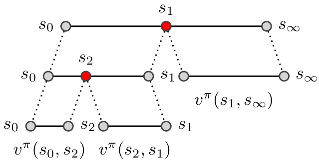
Figure 1. We propose a divide-and-conquer method to search for sub-goals (here $s_{1},s_{2})$ by hierarchical partitioning the task of guiding an agent from start state $s_{0}$ to goal state $s_{\infty}$ .

图 1: 我们提出一种分治法，通过分层划分从初始状态 $s_{0}$ 到目标状态 $s_{\infty}$ 的智能体引导任务，来搜索子目标 (此处为 $s_{1},s_{2}$)。

Most standard planners for sequential decision making problems—including Monte Carlo planning, Monte Carlo Tree Search (MCTS) and dynamic programming—have a baked-in sequential planning assumption (Browne et al., 2012; Bertsekas et al., 1995). These methods begin at either the initial or final state and then proceed to plan actions sequentially forward or backwards in time. However, this sequential approach faces two main challenges. (i) The transition model used for planning needs to be reliable over long horizons, which is often difficult to achieve when it has to be inferred from data. (ii) Credit assignment to each individual action is difficult: In a planning problem spanning a horizon of 100 steps, to assign credit to the first action, we have to compute the optimal cost-to-go for the remaining problem with a horizon of 99 steps, which is only slightly easier than solving the original problem.

大多数用于序列决策问题的标准规划器——包括蒙特卡洛规划、蒙特卡洛树搜索(MCTS)和动态规划——都内置了序列化规划假设 (Browne et al., 2012; Bertsekas et al., 1995)。这些方法从初始状态或最终状态出发，按时间顺序向前或向后逐步规划动作。但该序列化方法面临两大挑战：(i) 规划所用的转移模型需在长时域内保持可靠，当模型需从数据推断时往往难以实现；(ii) 单个动作的信用分配困难：在跨越100步的规划问题中，要为第一个动作分配信用，需计算剩余99步问题的最优成本，其难度仅略低于求解原问题。

To overcome these two fundamental challenges, we consider alternatives to the basic assumptions of sequential planners in this work. To this end, we focus on goal-directed decision making problems where an agent should reach a goal state from a start state. Instead of a transition and reward model of the environment, we assume a given goal-directed policy (the “low-level” policy) and the associated value oracle that returns the success probability of the low-level policy on any given task. In general, a low-level policy will not be not optimal, e.g. it might be too “myopic” to reliably reach goal states that are far away from its current state. We now seek to improve the low-level policy via a suitable sequence of subgoals that effectively guide it from the start to the final goal, thus maximizing the overall task success probability. This formulation of planning as finding good sub-goal sequences, makes learning of explicit environment models unnecessary, as they are replaced by low-level policies and their value functions.

为克服这两个根本性挑战，本研究重新审视序列规划器的基本假设。我们聚焦于目标导向型决策问题，即智能体需从初始状态抵达目标状态。不同于传统环境转移与奖励模型，我们采用给定目标导向策略（"底层"策略）及其关联的价值预言机——该预言机能返回底层策略在任何任务上的成功概率。由于底层策略通常并非最优（例如可能因"短视"而难以可靠到达远距离目标状态），我们通过构建合适的子目标序列来优化策略，从而有效引导其从起点抵达最终目标，实现整体任务成功概率最大化。这种将规划问题转化为子目标序列搜索的范式，消除了显式环境模型的学习需求，转而依赖底层策略及其价值函数实现决策。

The sub-goal planning problem can still be solved by a conventional sequential planner that begins by searching for the first sub-goal to reach from the start state, then planning the next sub-goal in sequence, and so on. Indeed, this is the approach taken in most hierarchical RL settings based on options or sub-goals (e.g. Dayan & Hinton, 1993; Sutton et al., 1999; Vezhnevets et al., 2017). However, the credit assignment problem mentioned above still persists, as assessing if the first sub-goal is useful still requires evaluating the success probability of the remaining plan. Instead, it could be substantially easier to reason about the utility of a sub-goal “in the middle” of the plan, as this breaks the long-horizon problem into two sub-problems with much shorter horizons: how to get to the sub-goal and how to get from there to the final goal. Based on this intuition, we propose the Divide-and-Conquer MCTS (DC-MCTS) planner that searches for sub-goals to split the original task into two independent sub-tasks of comparable complexity and then recursively solves these, thereby drastically facilitating credit assignment. To search the space of intermediate subgoals efficiently, DC-MCTS uses a heuristic for proposing promising sub-goals that is learned from previous search results and agent experience.

子目标规划问题仍可通过传统的顺序规划器解决，该规划器首先搜索从初始状态需达成的第一个子目标，随后依次规划后续子目标。事实上，这是大多数基于选项或子目标的层次强化学习（如 Dayan & Hinton, 1993; Sutton et al., 1999; Vezhnevets et al., 2017）采用的方法。然而，上述信用分配问题依然存在，因为评估首个子目标的有效性仍需考量剩余计划的成功概率。相比之下，分析计划"中间"子目标的效用可能更为简便——这将长视野问题拆解为两个视野更短的子问题：如何抵达该子目标，以及如何从该处到达最终目标。基于此直觉，我们提出分治蒙特卡洛树搜索（DC-MCTS）规划器，通过搜索子目标将原始任务分解为两个复杂度相当的独立子任务并递归求解，从而极大简化信用分配。为高效探索中间子目标空间，DC-MCTS采用启发式方法提出潜在子目标，该启发式通过先前的搜索结果和智能体经验学习获得。

The paper is structured as follows. In Section 2, we formulate planning in terms of sub-goals instead of primitive actions. In Section 3, as our main contribution, we propose the novel Divide-and-Conquer Monte Carlo Tree Search algorithm for this planning problem. In Section 5, we show that it outperforms sequential planners both on grid world and continuous control navigation tasks, demonstrating the utility of constructing plans in a flexible order that can be different from their execution order.

本文结构如下。第2节将规划问题表述为子目标而非原始动作。第3节作为主要贡献，针对该规划问题提出了新颖的分治蒙特卡洛树搜索算法。第5节通过网格世界和连续控制导航任务的实验表明，该算法性能优于顺序规划器，验证了以不同于执行顺序的灵活方式构建规划方案的实用性。

2. Improving Goal-Directed Policies with Planning

2. 通过规划改进目标导向策略

Let $s$ and $\mathcal{A}$ be finite sets of states and actions. We consider a multi-task setting, where for each episode the agent has to solve a new task consisting of a new Markov Decision Process (MDP) $\mathcal{M}$ over $s$ and $\mathcal{A}$ . Each $\mathcal{M}$ has a single start state $s_{0}$ and a special absorbing state $s_{\infty}$ , also termed the goal state. If the agent transitions into $s_{\infty}$ at any time it receives a reward of 1 and the episode terminates; otherwise the reward is 0. We assume that the agent observes the start and goal states $(s_{0},s_{\infty})$ at the beginning of each episode, as well as an encoding vector $c_{\mathcal{M}}\in\mathbb{R}^{d}$ . This vector provides the agent with additional information about the MDP $\mathcal{M}$ of the current episode and will be key to transfer learning across tasks in the multi-task setting. A stochastic, goal-directed policy $\pi$ is a mapping from $S\times S\times\mathbb{R}^{d}$ into distributions over $\mathcal{A}$ , where $\pi({a}|s,s_{\infty},c_{\mathcal{M}})$ denotes the probability of taking action $a$ in state $s$ in order to get to goal $s_{\infty}$ . For a fixed goal $s_{\infty}$ , we can interpret $\pi$ as a regular policy, here denoted as $\pi_{s_{\infty}}$ , mapping states to action probabilities. We denote the value of $\pi$ in state $s$ for goal $s_{\infty}$ as $v^{\pi}(s,s_{\infty}|c_{\mathcal{M}})$ ; we assume no discounting $\gamma=1$ . Under the above definition of the reward, the value is equal to the success probability of $\pi$ on the task, i.e. the absorption probability of the stochastic process starting in $s_{0}$ defined by running $\pi_{s_{\infty}}$ :

设 $s$ 和 $\mathcal{A}$ 为有限的状态集和动作集。我们考虑一个多任务场景，其中每个回合智能体需要解决一个新任务，该任务由在 $s$ 和 $\mathcal{A}$ 上定义的新马尔可夫决策过程 (MDP) $\mathcal{M}$ 组成。每个 $\mathcal{M}$ 有一个初始状态 $s_{0}$ 和一个特殊的吸收状态 $s_{\infty}$，也称为目标状态。如果智能体在任何时刻转移到 $s_{\infty}$，它将获得奖励 1 且回合终止；否则奖励为 0。我们假设智能体在每回合开始时观察初始和目标状态 $(s_{0},s_{\infty})$，以及一个编码向量 $c_{\mathcal{M}}\in\mathbb{R}^{d}$。该向量为智能体提供关于当前回合 MDP $\mathcal{M}$ 的额外信息，这将是多任务场景中跨任务迁移学习的关键。一个随机的、目标导向的策略 $\pi$ 是从 $S\times S\times\mathbb{R}^{d}$ 到 $\mathcal{A}$ 上概率分布的映射，其中 $\pi({a}|s,s_{\infty},c_{\mathcal{M}})$ 表示在状态 $s$ 中采取动作 $a$ 以达到目标 $s_{\infty}$ 的概率。对于一个固定的目标 $s_{\infty}$，我们可以将 $\pi$ 解释为一个常规策略，这里记为 $\pi_{s_{\infty}}$，它将状态映射到动作概率。我们将 $\pi$ 在状态 $s$ 对于目标 $s_{\infty}$ 的值记为 $v^{\pi}(s,s_{\infty}|c_{\mathcal{M}})$；我们假设无折扣 $\gamma=1$。在上述奖励定义下，该值等于 $\pi$ 在任务上的成功概率，即由运行 $\pi_{s_{\infty}}$ 定义的从 $s_{0}$ 开始的随机过程的吸收概率：

$$
v^{\pi}(s_{0},s_{\infty}|c_{\mathcal{M}})=P(s_{\infty}\in\tau_{s_{0}}^{\pi_{s_{\infty}}}|c_{\mathcal{M}}),
$$

where τ sπ0s∞ is the trajectory generated by running πs from state $s_{0}$ 1. To keep the notation compact, we will omit the explicit dependence on $c_{\mathcal{M}}$ and abbreviate tasks with pairs of states in $s\times s$ .

其中τ sπ0s∞是从状态$s_{0}$开始执行πs生成的轨迹。为简化表示，我们将省略对$c_{\mathcal{M}}$的显式依赖，并用状态对$s\times s$来缩写任务。

2.1. Planning over Sub-Goal Sequences

2.1. 子目标序列规划

Assume a given goal-directed policy $\pi$ , which we also refer to as the low-level policy. If $\pi$ is not already the optimal policy, then we can potentially improve it by planning: If $\pi$ has a low probability of directly reaching $s_{\infty}$ from the initial state $s_{0}$ , i.e. $v^{\pi}(s_{0},s_{\infty})\approx0$ , we will try to find a plan consisting of a sequence of intermediate sub-goals such that they guide $\pi$ from the start $s_{0}$ to the goal state $s_{\infty}$ .

假设给定一个目标导向的策略 $\pi$ ，我们也称之为低级策略。如果 $\pi$ 还不是最优策略，那么我们可以通过规划来改进它：如果 $\pi$ 从初始状态 $s_{0}$ 直接到达 $s_{\infty}$ 的概率较低，即 $v^{\pi}(s_{0},s_{\infty})\approx0$ ，我们将尝试找到一个由一系列中间子目标组成的计划，以引导 $\pi$ 从起始状态 $s_{0}$ 到达目标状态 $s_{\infty}$ 。

Concretely, let $S^{ * }=\cup_{n=0}^{\infty}S^{n}$ be the set of sequences over $s$ , and let $|\sigma|$ be the length of a sequence $\sigma\in S^{ * }$ . We define for convenience $\bar{\mathcal{S}}:=\mathcal{S}\cup{\varnothing}$ , where $\mathcal{D}$ is them empty sequence representing no sub-goal. We refer to $\sigma$ as a plan for task $(s_{0},s_{\infty})$ if $\sigma_{1}=s_{0}$ and $\sigma_{|\sigma|}=s_{\infty}$ , i.e. if the first and last elements of $\sigma$ are equal to $s_{0}$ and $s_{\infty}$ , respectively. We denote the set of plans for this task as $s_{0}S^{*}s_{\infty}$ .

具体地，设 $S^{ * }=\cup_{n=0}^{\infty}S^{n}$ 为 $s$ 上的序列集合，$|\sigma|$ 表示序列 $\sigma\in S^{ * }$ 的长度。为方便起见，定义 $\bar{\mathcal{S}}:=\mathcal{S}\cup{\varnothing}$ ，其中 $\mathcal{D}$ 是表示无子目标的空序列。若序列 $\sigma$ 满足 $\sigma_{1}=s_{0}$ 且 $\sigma_{|\sigma|}=s_{\infty}$ （即首尾元素分别等于 $s_{0}$ 和 $s_{\infty}$ ），则称 $\sigma$ 为任务 $(s_{0},s_{\infty})$ 的规划。该任务的所有规划集合记为 $s_{0}S^{*}s_{\infty}$。

To execute a plan $\sigma$ , we construct a policy $\pi_{\sigma}$ by conditioning the low-level policy $\pi$ on each of the sub-goals in order: Starting with $n=1$ , we feed sub-goal $\sigma_{n+1}$ to $\pi$ , i.e. we run $\pi_{\sigma_{n+1}}$ ; if $\sigma_{n+1}$ is reached, we will execute $\pi_{\sigma_{n+2}}$ and so on. We now wish to do open-loop planning, i.e. find the plan with the highest success probability $P(s_{\infty}\in\tau_{s_{0}}^{\pi_{\sigma}})$ of reaching $s_{\infty}$ . However, this success probability depends on the transition kernels of the underlying MPDs, which might not be known. We can instead define planning as maximizing the following lower bound of the success probability, that can be expressed in terms of the low-level value $v^{\pi}$ .

要执行一个计划 $\sigma$，我们通过按顺序将低层策略 $\pi$ 条件化到每个子目标上来构建策略 $\pi_{\sigma}$：从 $n=1$ 开始，我们将子目标 $\sigma_{n+1}$ 输入给 $\pi$，即运行 $\pi_{\sigma_{n+1}}$；如果达到 $\sigma_{n+1}$，则继续执行 $\pi_{\sigma_{n+2}}$，依此类推。现在，我们希望进行开环规划 (open-loop planning)，即找到达到 $s_{\infty}$ 的成功概率 $P(s_{\infty}\in\tau_{s_{0}}^{\pi_{\sigma}})$ 最高的计划。然而，这一成功概率取决于底层 MPD 的转移核，而这些可能未知。于是，我们可以将规划定义为最大化以下成功概率的下界，该下界可以用低层价值 $v^{\pi}$ 表示。

Proposition 1 (Lower bound of success probability). The success probability $P(s_{\infty}\in\tau_{s_{0}}^{\pi_{\sigma}})\geq L(\sigma)$ of a plan $\sigma$ is bounded from below by $\begin{array}{r}{L(\sigma):=\prod_{i=1}^{|\sigma|-1}v^{\pi}(\sigma_{i},\sigma_{i+1}),}\end{array}$ i.e. the product of the success probab ilities of $\pi$ on the subtasks defined by $(\sigma_{i},\sigma_{i+1})$ .

命题1 (成功概率下界). 计划$\sigma$的成功概率$P(s_{\infty}\in\tau_{s_{0}}^{\pi_{\sigma}})\geq L(\sigma)$存在下界$\begin{array}{r}{L(\sigma):=\prod_{i=1}^{|\sigma|-1}v^{\pi}(\sigma_{i},\sigma_{i+1}),}\end{array}$, 即$\pi$在子任务$(\sigma_{i},\sigma_{i+1})$上成功概率的乘积。

The straight-forward proof is given in Appendix A.1. Intuitively, $L(\sigma)$ is a lower bound for the success of $\pi_{\sigma}$ , as it neglects the probability of “accidentally” (due to stochasticity of the policy or transitions) running into the goal $s_{\infty}$ before having executed the full plan. We summarize:

直观证明见附录A.1。从直观上看，$L(\sigma)$是$\pi_{\sigma}$成功概率的下界，因为它忽略了在完整执行计划前"意外"(由于策略或状态转移的随机性)抵达目标状态$s_{\infty}$的概率。我们总结如下：

Definition 1 (Open-Loop Goal-Directed Planning). Given a goal-directed policy $\pi$ and its corresponding value oracle $v^{\pi}$ , we define planning as optimizing $L(\sigma)$ over $\sigma\in$ $s_{0}S^{ * }s_{\infty}$ , i.e. the set of plans for task $(s_{0},s_{\infty})$ . We define the high-level (HL) value $v^{ * }(s_{0},s_{\infty}):=\operatorname*{max}_{\sigma}L(\sigma)$ as the maximum value of the planning objective.

定义 1 (开环目标导向规划) 。给定目标导向策略 $\pi$ 及其对应的价值预言机 $v^{\pi}$ ，我们将规划定义为在 $\sigma\in$ $s_{0}S^{ * }s_{\infty}$ (即任务 $(s_{0},s_{\infty})$ 的计划集合) 上优化 $L(\sigma)$ 。我们将高层 (HL) 价值 $v^{ * }(s_{0},s_{\infty}):=\operatorname*{max}_{\sigma}L(\sigma)$ 定义为规划目标的最大值。

Note the difference between the low-level value $v^{\pi}$ and the high-level $v^{ * }$ . $v^{\pi}(s,s^{\prime})$ is the probability of the agent directly reaching $s^{\prime}$ from $s$ following $\pi$ , whereas $v^{ * }(s,s^{\prime})$ the probability reaching $s^{\prime}$ from $s$ under the optimal plan, which likely includes intermediate sub-goals. In particular we have $v^{*}\geq v^{\pi}$ .

注意低层值 $v^{\pi}$ 和高层值 $v^{ * }$ 之间的区别。$v^{\pi}(s,s^{\prime})$ 是智能体遵循策略 $\pi$ 直接从 $s$ 到达 $s^{\prime}$ 的概率，而 $v^{ * }(s,s^{\prime})$ 是在最优计划下从 $s$ 到达 $s^{\prime}$ 的概率，其中可能包含中间子目标。特别地，我们有 $v^{*}\geq v^{\pi}$。

2.2. AND/OR Search Tree Representation

2.2. AND/OR 搜索树表示

In the following we cast the planning problem into a representation amenable to efficient search. To this end, we use the natural compositional it y of plans: We can concatenate, a plan $\sigma$ for the task $(s,s^{\prime})$ and a plan $\hat{\sigma}$ for the task $(s^{\prime},s^{\prime\prime})$ into a plan $\sigma\circ\hat{\sigma}$ for the task $(s,s^{\prime\prime})$ . Conversely, we can decompose any given plan $\sigma$ for task $(s_{0},s_{\infty})$ by splitting it at any sub-goal $s\in\sigma$ into $\sigma=\sigma^{l}\circ\sigma^{r}$ , where $\sigma^{l}$ is the “left” sub-plan for task $(s_{0},s)$ , and $\sigma^{r}$ is the “right” sub-plan for task $(s,s_{\infty})$ . For an illustration see Figure 1. Trivially, the planning objective and the optimal high-level value factorize wrt. to this decomposition:

以下我们将规划问题转化为适合高效搜索的表示形式。为此，我们利用规划的自然组合性：可以将任务$(s,s^{\prime})$的规划$\sigma$与任务$(s^{\prime},s^{\prime\prime})$的规划$\hat{\sigma}$拼接成任务$(s,s^{\prime\prime})$的规划$\sigma\circ\hat{\sigma}$。反之，对于任务$(s_{0},s_{\infty})$的任意给定规划$\sigma$，可通过在子目标$s\in\sigma$处将其拆分为$\sigma=\sigma^{l}\circ\sigma^{r}$，其中$\sigma^{l}$是任务$(s_{0},s)$的"左"子规划，$\sigma^{r}$是任务$(s,s_{\infty})$的"右"子规划。示意图见图1。显然，规划目标与最优高层价值函数均关于该分解具有可乘性：

$$
\begin{array}{l c l}{{{\cal L}(\sigma^{l}\circ\sigma^{r})}}&{{=}}&{{{\cal L}(\sigma^{l}){\cal L}(\sigma^{r})}}\ {{v^{ * }(s_{0},s_{\infty})}}&{{=}}&{{\displaystyle\operatorname*{max}_ {s\in\bar{S}}v^{ * }(s_{0},s)\cdot v^{*}(s,s_{\infty}).}}\end{array}
$$

This allows us to recursively reformulate planning as:

这使我们能够递归地将规划重新表述为：

$$
\underset{s\in\bar{\cal S}}{\arg\operatorname*{max}}\left(\arg\operatorname*{max}_ {\sigma_{l}\in s_{0}}L(\sigma^{l})\right)\cdot\left(\arg\operatorname*{max}_ {\sigma_{r}\in s{\cal S}^{\ast}s_{\infty}}L(\sigma^{r})\right).
$$

The above equations are the Bellman equations and the Bellman optimality equations for the classical single pair shortest path problem in graphs, where the edge weights are given by $-\log v^{\pi}(s,s^{\prime})$ . We can represent this planning problem by an AND/OR search tree (Nilsson, N. J., 1980) consisting of alternating levels of OR and AND nodes. An OR node, also termed an action node, is labeled by a task $(s,s^{\prime\prime})\in\boldsymbol{\mathcal{S}}\times\boldsymbol{\mathcal{S}}$ ; the root of the search tree is an OR node labeled by the original task $(s_{0},s_{\infty})$ . A terminal OR node $(s,s^{\prime\prime})$ has a value $v^{\pi}(s,s^{\prime\prime})$ attached to it, which reflects the success probability of $\pi_{s^{\prime\prime}}$ for completing the sub-task $(s,s^{\prime\prime})$ . Each non-terminal OR node has $|S|+1$ AND nodes as children. Each of these is labeled by a triple $(s,s^{\prime},s^{\prime\prime})$ for $s^{\prime}\in\bar{S}$ , which correspond to inserting a sub-goal $s^{\prime}$ into the overall plan, or not inserting one in case of $s=\emptyset$ Every AND node $(s,s^{\prime},s^{\prime\prime})$ , which we will also refer to as a conjunction node, has two OR children, the “left” sub-task $(s,s^{\prime})$ and the “right” sub-task $(s^{\prime},s^{\prime\prime})$ .

上述方程是图中经典单对最短路径问题的贝尔曼方程和贝尔曼最优性方程，其中边权重由 $-\log v^{\pi}(s,s^{\prime})$ 给出。我们可以通过一个由交替的OR节点和AND节点层级组成的AND/OR搜索树 (Nilsson, N. J., 1980) 来表示这一规划问题。OR节点（也称为动作节点）由任务 $(s,s^{\prime\prime})\in\boldsymbol{\mathcal{S}}\times\boldsymbol{\mathcal{S}}$ 标记；搜索树的根节点是由原始任务 $(s_{0},s_{\infty})$ 标记的OR节点。终端OR节点 $(s,s^{\prime\prime})$ 附有一个值 $v^{\pi}(s,s^{\prime\prime})$ ，它反映了 $\pi_{s^{\prime\prime}}$ 完成子任务 $(s,s^{\prime\prime})$ 的成功概率。每个非终端OR节点有 $|S|+1$ 个AND子节点，每个子节点由三元组 $(s,s^{\prime},s^{\prime\prime})$ （其中 $s^{\prime}\in\bar{S}$ ）标记，对应于在整体计划中插入子目标 $s^{\prime}$ ，或在 $s=\emptyset$ 时不插入。每个AND节点 $(s,s^{\prime},s^{\prime\prime})$ （也称为合取节点）有两个OR子节点，即“左”子任务 $(s,s^{\prime})$ 和“右”子任务 $(s^{\prime},s^{\prime\prime})$ 。

In this representation, plans are induced by solution trees. A solution tree $\mathcal{T}_ {\sigma}$ is a sub-tree of the complete AND/OR search tree, with the properties that (i) the root $(s_{0},s_{\infty})\in$ $\mathcal{T}_ {\sigma}$ , (ii) each OR node in $\tau_{\sigma}$ has at most one child in $\mathcal{T}_ {\sigma}$ and (iii) each AND node in $\mathcal{T}_ {\sigma}$ as two children in $\mathcal{T}_ {\sigma}$ . The plan $\sigma$ and its objective $L(\sigma)$ can be computed from $\tau_{\sigma}$ by a depth-first traversal of $\tau_{\sigma}$ , see Figure 1. The correspondence of sub-trees to plans is many-to-one, as $\tau_{\sigma}$ , in addition to the plan itself, contains the order in which the plan was constructed. Figure 6 in the Appendix shows a example for a search and solution tree. Below we will discuss how to construct a favourable search order heuristic.

在此表示中，计划由解树推导得出。解树 $\mathcal{T}_ {\sigma}$ 是完整AND/OR搜索树的子树，具有以下特性：(i) 根节点 $(s_{0},s_{\infty})\in$ $\mathcal{T}_ {\sigma}$，(ii) $\tau_{\sigma}$ 中的每个OR节点在 $\mathcal{T}_ {\sigma}$ 中至多有一个子节点，(iii) $\mathcal{T}_ {\sigma}$ 中的每个AND节点在 $\mathcal{T}_ {\sigma}$ 中有两个子节点。计划 $\sigma$ 及其目标值 $L(\sigma)$ 可通过深度优先遍历 $\tau_{\sigma}$ 计算得出，如图1所示。子树与计划的对应关系是多对一的，因为 $\tau_{\sigma}$ 除了包含计划本身外，还包含计划的构建顺序。附录中的图6展示了搜索树与解树的示例。下文将讨论如何构建有利的搜索顺序启发式策略。

3. Best-First AND/OR Planning

3. 最佳优先与或规划

The planning problem from Definition 1 can be solved exactly by formulating it as shortest path problem from $s_{0}$ to $s_{\infty}$ on a fully connected graph with vertex set $s$ with non-negative edge weights given by $-\log v^{\pi}$ and applying a classical Single Source or All Pairs Shortest Path (SSSP / APSP) planner. This approach is appropriate if one wants to solve all goal-directed tasks in a single MDP. Here, we focus however on the multi-task setting described above, where the agent is given a new MDP wit a single task $(s_{0},s_{\infty})$ every episode. In this case, solving the ${\tt S S S P}/$ APSP problem is not feasible: Tabulating all graphs weights $-\log v^{\pi}(s,s^{\prime})$ would require $|\boldsymbol{S}|^{2}$ evaluations of $v^{\pi}(s,s^{\prime})$ for all pairs $(s,s^{\prime})$ . In practice, approximate evaluations of $v^{\pi}$ could be implemented by e.g. actually running the policy $\pi$ , or by calls to a powerful function approx im at or, both of which are often too costly to exhaustively evaluate for large state-spaces $s$ . Instead, we tailor an algorithm for approximate planning to the multi-task setting, which we call Divide-and-Conquer MCTS (DC-MCTS). To evaluate $v^{\pi}$ as sparsely as possible, DC-MCTS critically makes use of two learned search heuristics that transfer knowledge from previously encountered MDPs / tasks to new problem instance: (i) a distribution $p(s^{\prime}|s,s^{\prime\prime})$ , called the policy prior, for proposing promising intermediate sub-goals $s^{\prime}$ for a task $(s,s^{\prime\prime})$ ; and (ii) a learned approximation $v$ to the high-level value $v^{*}$ for bootstrap evaluation of partial plans. In the following we present DC-MCTS and discuss design choices and training for the two search heuristics.

根据定义1，规划问题可以通过将其表述为从$s_{0}$到$s_{\infty}$的最短路径问题来精确求解，该问题基于一个完全连通的图结构，其中顶点集为$s$，边权重由$-\log v^{\pi}$给出且非负，并应用经典的单源或全对最短路径（SSSP/APSP）规划器。这种方法适用于需要在一个MDP中解决所有目标导向任务的情况。然而，本文重点讨论上述多任务场景，其中智能体每回合会收到一个包含单一任务$(s_{0},s_{\infty})$的新MDP。此时，求解${\tt SSSP}/$APSP问题不可行：若对所有状态对$(s,s^{\prime})$制表$-\log v^{\pi}(s,s^{\prime})$，则需进行$|\boldsymbol{S}|^{2}$次$v^{\pi}(s,s^{\prime})$评估。实践中，可通过实际运行策略$\pi$或调用强大的函数逼近器来近似评估$v^{\pi}$，但对于大规模状态空间$s$，这两种方法往往因计算成本过高而难以穷举。为此，我们针对多任务场景定制了近似规划算法——分治蒙特卡洛树搜索（DC-MCTS）。为尽可能稀疏地评估$v^{\pi}$，DC-MCTS关键性地利用了两个从历史MDP/任务迁移知识的搜索启发式：(i) 策略先验分布$p(s^{\prime}|s,s^{\prime\prime})$，用于为任务$(s,s^{\prime\prime})$推荐潜在中间子目标$s^{\prime}$；(ii) 对高层价值$v^{*}$的学习近似$v$，用于部分规划的自举评估。下文将介绍DC-MCTS，并讨论两个搜索启发式的设计选择与训练过程。

Algorithm1 Divide-and-Conquer MCTSprocedures

Global low-level value oracle vm

Globalhigh-level value function v

Global policy prior p

Global search tree T

1: procedure TRAVERSE(OR node (s, s"))

2: if (s, s") T then

3: T← ExPAND(T,(s, s"))

4: return max(u"(s, s"),v(s, s")) bootstrap

5: end if

6: s'← SELECT(s, s") OR node

7: if s' = or max-depth reached then

8: G←u"(s, s"")

9: else > AND node

10: Gleft ← TRAVERSE(s, s')

11: Gright ← TRAVERSE(s', s")

12: // BACKUP

13: G← Gleft · Gright

14: end if

15: G← max(G,v"(s, s")) threshold the return

16: //UPDATE

17: V(s, s") < (V(s, s")N(s, s")+G)/(N(s, s")+1)

18: N(s, s") ← N(s,s") + 1

19: return G

20: end procedure

算法1 分治MCTS流程
全局低层价值评估器 vm
全局高层价值函数 v
全局策略先验 p
全局搜索树 T
1: 过程 TRAVERSE(或节点 (s, s"))
2: 如果 (s, s") 不在 T 中
3: T← 扩展(T,(s, s"))
4: 返回 max(u"(s, s"),v(s, s")) 自举值
5: 结束条件
6: s'← 选择(s, s") 或节点
7: 如果 s' = 空或达到最大深度
8: G←u"(s, s"")
9: 否则 > 与节点
10: G左 ← 遍历(s, s')
11: G右 ← 遍历(s', s")
12: // 回传
13: G← G左 · G右
14: 结束条件
15: G← max(G,v"(s, s")) 阈值化返回值
16: //更新
17: V(s, s") ← (V(s, s")N(s, s")+G)/(N(s, s")+1)
18: N(s, s") ← N(s,s") + 1
19: 返回 G
20: 结束过程

3.1. Divide-and-Conquer Monte Carlo Tree Search

3.1. 分治蒙特卡洛树搜索

The input to the DC-MCTS planner is an MDP encoding $c_{\mathcal{M}}$ , a task $(s_{0},s_{\infty})$ as well as a planning budget, i.e. a maximum number $B\in\mathbb{N}$ of $v^{\pi}$ oracle evaluations. At each stage, DC-MCTS maintains a (partial) AND/OR search tree $\tau$ whose root is the OR node $(s_{0},s_{\infty})$ corresponding to the original task. Every OR node $(s,s^{\prime\prime})\in\mathcal{T}$ maintains an estimate $V(s,s^{\prime\prime})\approx v^{*}(s,s^{\prime\prime})$ of its high-level value. DC-MCTS searches for a plan by iterative ly constructing the search tree $\tau$ with TRAVERSE until the budget is exhausted, see Algorithm 1. During each traversal, if a leaf node of $\tau$ is reached, it is expanded, followed by a recursive bottom-up backup to update the value estimates $V$ of all OR nodes visited in this traversal. After this search phase, the currently best plan is extracted from $\tau$ by EXTRACTPLAN (essentially depth-first traversal, see Algorithm 2 in the Appendix). In the following we briefly describe the main methods of the search.

DC-MCTS规划器的输入是一个MDP编码$c_{\mathcal{M}}$、任务$(s_{0},s_{\infty})$以及规划预算(即$v^{\pi}$预言评估的最大次数$B\in\mathbb{N}$)。在每一阶段，DC-MCTS维护一个(部分)AND/OR搜索树$\tau$，其根节点是对应原始任务的OR节点$(s_{0},s_{\infty})$。每个OR节点$(s,s^{\prime\prime})\in\mathcal{T}$维护着其高层价值估计$V(s,s^{\prime\prime})\approx v^{*}(s,s^{\prime\prime})$。DC-MCTS通过迭代构建搜索树$\tau$(使用TRAVERSE算法)来寻找规划方案，直至预算耗尽(见算法1)。每次遍历期间，若到达$\tau$的叶节点，则对其进行扩展，随后通过递归自底向上回溯来更新本次遍历中访问的所有OR节点的价值估计$V$。搜索阶段结束后，通过EXTRACTPLAN(本质上是深度优先遍历，见附录算法2)从$\tau$中提取当前最优规划方案。下文将简要介绍搜索的主要方法。

TRAVERSE and SELECT $\tau$ is traversed from the root $(s_{0},s_{\infty})$ to find a promising node to expand. At an OR node $(s,s^{\prime\prime})$ , SELECT chooses one of its children $s^{\prime}\in\bar{S}$ to next traverse into, including $s=\emptyset$ for not inserting any further sub-goals into this branch. We implemented SELECT by the pUCT (Rosin, 2011) rule, which consists of picking the next node $s^{\prime}\in\bar{S}$ based on maximizing the following score:

遍历与选择
从根节点 $(s_{0},s_{\infty})$ 开始遍历 $\tau$ 以寻找有扩展潜力的节点。在OR节点 $(s,s^{\prime\prime})$ 处，SELECT会从其子节点 $s^{\prime}\in\bar{S}$ 中选择一个进行下一步遍历（包括 $s=\emptyset$ 表示不再向该分支插入子目标）。我们采用pUCT规则 (Rosin, 2011) 实现SELECT，其核心是通过最大化以下评分来选择下一个节点 $s^{\prime}\in\bar{S}$：

$$
V(s,s^{\prime})\cdot V(s^{\prime},s^{\prime\prime})+c\cdot p(s^{\prime}|s,s^{\prime\prime})\cdot\frac{\sqrt{N(s,s^{\prime\prime})}}{1+N(s,s^{\prime},s^{\prime\prime})},
$$

where $N(s,s^{\prime})$ , $N(s,s^{\prime},s^{\prime\prime})$ are the visit counts of the OR node $(s,s^{\prime})$ , AND node $(s,s^{\prime},s^{\prime\prime})$ respectively. The first term is the exploitation component, guiding the search to sub-goals that currently look promising, i.e. have high estimated value. The second term is the exploration term favoring nodes with low visit counts. Crucially, it is explicitly scaled by the policy prior $p(s^{\prime}|s,s^{\prime\prime})$ to guide exploration. At an AND node $(s,s^{\prime},s^{\prime\prime})$ , TRAVERSE traverses into both the left $(s,s^{\prime})$ and right child $(s^{\prime},s^{\prime\prime})$ .2 As the two subproblems are solved independently, computation from there on can be carried out in parallel. All nodes visited in a single traversal form a solution tree denoted here as $\tau_{\sigma}$ with plan $\sigma$ .

其中 $N(s,s^{\prime})$ 和 $N(s,s^{\prime},s^{\prime\prime})$ 分别是 OR 节点 $(s,s^{\prime})$ 和 AND 节点 $(s,s^{\prime},s^{\prime\prime})$ 的访问计数。第一项是开发(exploitation)部分，引导搜索到当前看起来有前景的子目标，即具有较高估计值的子目标。第二项是探索(exploration)部分，倾向于访问计数较低的节点。关键的是，它通过策略先验 $p(s^{\prime}|s,s^{\prime\prime})$ 显式缩放以引导探索。在 AND 节点 $(s,s^{\prime},s^{\prime\prime})$ 处，TRAVERSE 会同时遍历左子节点 $(s,s^{\prime})$ 和右子节点 $(s^{\prime},s^{\prime\prime})$。由于这两个子问题是独立求解的，后续计算可以并行进行。单次遍历中访问的所有节点形成一个解树，记为 $\tau_{\sigma}$，其对应计划为 $\sigma$。

EXPAND If a leaf OR node $(s,s^{\prime\prime})$ is reached during the traversal and its depth is smaller than a given maximum depth, it is expanded by evaluating the high- and low-level values $v(s,s^{\prime\prime})$ , $v^{\pi}(s,s^{\prime\prime})$ . The initial value of the node is defined as max of both values, as by definition $v^{*}\geq$ $v^{\pi}$ , i.e. further planning should only increase the success probability on a sub-task. We also evaluate the policy prior $p(s^{\prime}|s,s^{\prime\prime})$ for all $s^{\prime}$ , yielding the proposal distribution over sub-goals used in SELECT. Each node expansion costs one unit of budget $B$ .

EXPAND 如果在遍历过程中到达一个叶节点或节点 $(s,s^{\prime\prime})$ 且其深度小于给定的最大深度，则通过评估高层次和低层次值 $v(s,s^{\prime\prime})$ 、 $v^{\pi}(s,s^{\prime\prime})$ 来扩展该节点。节点的初始值定义为这两个值的最大值，因为根据定义 $v^{*}\geq$ $v^{\pi}$ ，即进一步的规划应仅增加子任务的成功概率。我们还会评估所有 $s^{\prime}$ 的策略先验 $p(s^{\prime}|s,s^{\prime\prime})$ ，生成用于SELECT的子目标提议分布。每次节点扩展消耗一个预算单位 $B$ 。

BACKUP and UPDATE We define the return $G_{\sigma}$ of the traversal tree $\tau_{\sigma}$ as follows. Let a refinement $\mathcal{T}_ {\sigma}^{+}$ of $\mathcal{T}_ {\sigma}$ be a solution tree such that ${\mathcal{T}}_ {\sigma}\subseteq{\mathcal{T}}_ {\sigma}^{+}$ , thus representing a plan $\sigma^{+}$ that has all sub-goals of $\sigma$ with additional inserted sub-goals. $G_{\sigma}$ is now defined as the value of the objective $L(\sigma^{+})$ of the optimal refinement of $\mathcal{T}_ {\sigma}$ , i.e. it reflects how well one could do on task $(s_{0},s_{\infty})$ by starting from the plan $\sigma$ and refining it. It can be computed by a simple back-up on the tree $\mathcal{T}_ {\sigma}$ that uses the bootstrap value $v\approx v^{ * }$ at the leafs. As $v^{\ast}(s_{0},s_{\infty})\geq G_{\sigma}\geq L(\sigma)$ and $G_{\sigma^{ * }}=v^{ * }(s_{0},s_{\infty})$ for the optimal plan $\sigma^{*}$ , we can use $G_{\sigma}$ to update the value estimate $V$ . Like in other MCTS variants, we employ a running average operation (line 17-18 in TRAVERSE).

备份与更新
我们将遍历树 $\tau_{\sigma}$ 的回报 $G_{\sigma}$ 定义如下。设 $\mathcal{T}_ {\sigma}$ 的一个细化 $\mathcal{T}_ {\sigma}^{+}$ 为满足 ${\mathcal{T}}_ {\sigma}\subseteq{\mathcal{T}}_ {\sigma}^{+}$ 的解树，表示一个包含 $\sigma$ 所有子目标并额外插入子目标的计划 $\sigma^{+}$。此时 $G_{\sigma}$ 定义为 $\mathcal{T}_ {\sigma}$ 最优细化的目标值 $L(\sigma^{+})$，即反映从计划 $\sigma$ 出发细化后能在任务 $(s_{0},s_{\infty})$ 上达到的最佳效果。它可通过在树 $\mathcal{T}_ {\sigma}$ 上执行简单备份计算得出，其中叶节点使用近似引导值 $v\approx v^{ * }$。由于对于最优计划 $\sigma^{ * }$ 有 $v^{\ast}(s_{0},s_{\infty})\geq G_{\sigma}\geq L(\sigma)$ 且 $G_{\sigma^{ * }}=v^{*}(s_{0},s_{\infty})$，我们可用 $G_{\sigma}$ 更新价值估计 $V$。与其他MCTS变体类似，我们采用滑动平均操作（TRAVERSE算法第17-18行）。

3.2. Designing and Training Search Heuristics

3.2. 设计和训练搜索启发式

Search results and experience from previous tasks can be used to improve DC-MCTS on new problem instances via adapting the search heuristics, i.e. the policy prior $p$ and the approximate value function $v$ , in the following way.

利用先前任务的搜索结果和经验，可通过以下方式调整搜索启发式策略（即策略先验 $p$ 和近似价值函数 $v$）来提升DC-MCTS在新问题实例上的表现。

Bootstrap Value Function We parametrize $v(s,s^{\prime}|c_{\mathcal{M}})\approx~v^{*}(s,s^{\prime}|c_{\mathcal{M}})$ as a neural network that takes as inputs the current task consisting of $(s,s^{\prime})$ and the MDP encoding $c_{\mathcal{M}}$ . A straight-forward approach to train $v$ is to regress it towards the non-parametric value estimates $V$ computed by DC-MCTS on previous problem instances. However, initial results indicated that this leads to $v$ being overly optimistic, an observation also made in (Kaelbling, 1993). We therefore used more conservative training targets, that are computed by backing the low-level values $v^{\pi}$ up the solution tree $\tau_{\sigma}$ of the plan $\sigma$ return by DC-MCTS. Details can be found in Appendix B.1.

Bootstrap值函数我们将$v(s,s^{\prime}|c_{\mathcal{M}})\approx~v^{*}(s,s^{\prime}|c_{\mathcal{M}})$参数化为一个神经网络，其输入包括当前任务$(s,s^{\prime})$和MDP编码$c_{\mathcal{M}}$。训练$v$的直接方法是将其回归到DC-MCTS在先前问题实例上计算的非参数值估计$V$。然而，初步结果表明这会导致$v$过于乐观，这一现象在 (Kaelbling, 1993) 中也有提及。因此，我们采用了更保守的训练目标，这些目标通过将底层值$v^{\pi}$沿DC-MCTS返回的计划$\sigma$的解树$\tau_{\sigma}$反向传播计算得出。详情见附录B.1。

Policy Prior Best-first search guided by a policy prior $p$ can be understood as policy improvement of $p$ as described in (Silver et al., 2016). Therefore, a straight-forward way of training $p$ is to distill the search results back into into the policy prior, e.g. by behavioral cloning. When applying this to DC-MCTS in our setting, we found empirically that this yielded very slow improvement when starting from an untrained, uniform prior $p$ . This is due to plans with non-zero success probability $L>0$ being very sparse in $S^{ * }$ , equivalent to the sparse reward setting in regular MDPs. To address this issue, we propose to apply Hindsight Experience Replay (HER, (An dry ch owicz et al., 2017)): Instead of training $p$ exclusively on search results, we additionally execute plans $\sigma$ in the environment and collect the resulting trajectories, i.e. the sequence of visited states, $\tau_{s_{0}}^{\pi_{\sigma}}=(s_{0},s_{1},...,s_{T})$ HER then proceeds with hindsight relabeling, i.e. taking $\tau_{s_{0}}^{\pi_{\sigma}}$ as an approximately optimal plan for the “fictional” task $(s_{0},s_{T})$ that is likely different from the actual task $(s_{0},s_{\infty})$ In standard HER, these fictitious expert demonstrations are used for imitation learning of goal-directed policies, thereby circumventing the sparse reward problem. We can apply HER to train $p$ in our setting by extracting any ordered triplet $(s_{t_{1}},s_{t_{2}},s_{t_{3}})$ from $\tau_{s_{0}}^{\pi_{\sigma}}$ and use it as supervised learning targets for $p$ . This is a sensible procedure, as $p$ would then learn to predict optimal sub-goals $s_{t_{2}}^{ * }$ for sub-tasks $(s_{t_{1}}^{ * },s_{t_{3}}^{ * })$ under the assumption that the data was generated by an oracle producing optimal plans $\tau_{s_{0}}^{\pi_{\sigma}}=\sigma^{*}$ .

策略先验
由策略先验 $p$ 引导的最佳优先搜索可以理解为对 $p$ 的策略改进 (如 Silver 等人 2016 年所述)。因此，训练 $p$ 的直接方法是将搜索结果反蒸馏回策略先验，例如通过行为克隆。当在我们的设置中将此方法应用于 DC-MCTS 时，我们通过实验发现，从未经训练的均匀先验 $p$ 开始时，这种方法产生的改进非常缓慢。这是由于在 $S^{*}$ 中，具有非零成功概率 $L>0$ 的计划非常稀疏，相当于常规 MDP 中的稀疏奖励设置。

为了解决这个问题，我们提出应用后见之明经验回放 (Hindsight Experience Replay, HER) (Andrychowicz 等人, 2017)：除了在搜索结果上训练 $p$ 外，我们还在环境中执行计划 $\sigma$ 并收集生成的轨迹，即访问状态的序列 $\tau_{s_{0}}^{\pi_{\sigma}}=(s_{0},s_{1},...,s_{T})$。随后，HER 进行后见之明重标记，即将 $\tau_{s_{0}}^{\pi_{\sigma}}$ 视为“虚构”任务 $(s_{0},s_{T})$ 的近似最优计划，该任务可能与实际任务 $(s_{0},s_{\infty})$ 不同。

在标准 HER 中，这些虚构的专家演示用于目标导向策略的模仿学习，从而规避稀疏奖励问题。我们可以通过从 $\tau_{s_{0}}^{\pi_{\sigma}}$ 中提取任意有序三元组 $(s_{t_{1}},s_{t_{2}},s_{t_{3}})$ 并将其用作 $p$ 的监督学习目标，从而在我们的设置中应用 HER 来训练 $p$。这是一个合理的操作，因为 $p$ 随后会学习在假设数据是由生成最优计划 $\tau_{s_{0}}^{\pi_{\sigma}}=\sigma^{ * }$ 的预言机生成的情况下，预测子任务 $(s_{t_{1}}^{ * },s_{t_{3}}^{ * })$ 的最优子目标 $s_{t_{2}}^{*}$。

We have considerable freedom in choosing which triplets to extract from data and use as supervision, which we can characterize in the following way. Given a task $(s_{0},s_{\infty})$ , the policy prior $p$ defines a distribution over binary partition trees of the task via recursive application (until the terminal symbol $\boldsymbol{\mathcal{O}}$ closes a branch). A sample $\mathcal{T}_ {\sigma}$ from this distribution implies a plan $\sigma$ as described above; but furthermore it also contains the order in which the task was partitioned. Therefore, $p$ not only implies a distribution over plans, but also a search order: Trees with high probability under $p$ will be discovered earlier in the search with DC-MCTS. For generating training targets for supervised training of $p$ , we need to parse a given sequence $\tau_{s_{0}}^{\pi_{\sigma}}=(s_{0},s_{1},\ldots,s_{T})$ into a binary tree. Therefore, when applying HER we are free to chose any deterministic or probabilistic parser that generates a solution tree $\mathcal{T}_ {\tau_{s_{0}}^{\pi_{\sigma}}}$ from re-label HER data $\tau_{s_{0}}^{\pi_{\sigma}}$ . The particular choice of HER-parser will shape the search strategy defined by $p$ . Possible choices include:

在选择从数据中提取哪些三元组作为监督信号时，我们拥有相当大的自由度，这可以通过以下方式描述。给定任务$(s_{0},s_{\infty})$，策略先验$p$通过递归应用（直到终止符号$\boldsymbol{\mathcal{O}}$关闭分支）定义了任务二叉划分树的分布。从该分布中采样的$\mathcal{T}_ {\sigma}$不仅隐含了上述计划$\sigma$，还包含了任务被划分的顺序。因此，$p$不仅定义了计划的分布，还定义了搜索顺序：在DC-MCTS搜索中，高概率的树会优先被发现。为了生成用于监督训练$p$的目标，我们需要将给定序列$\tau_{s_{0}}^{\pi_{\sigma}}=(s_{0},s_{1},\ldots,s_{T})$解析为二叉树。因此，在应用HER时，我们可以自由选择任何确定性或概率性解析器，从重新标记的HER数据$\tau_{s_{0}}^{\pi_{\sigma}}$生成解树$\mathcal{T}_ {\tau_{s_{0}}^{\pi_{\sigma}}}$。HER解析器的具体选择将塑造由$p$定义的搜索策略。可能的选项包括：

相关工作

Goal-directed multi-task learning has been identified as an important special case of general RL and has been extensively studied. Universal value functions (Schaul et al., 2015) have been established as compact representation for this setting (Kulkarni et al., 2016; An dry ch owicz et al., 2017; Ghosh et al., 2018; Dhiman et al., 2018). This allows to use sub-goals as means for planning, as done in several works such as (Kaelbling & Lozano-Pérez, 2017; Gao et al., 2017; Savinov et al., 2018; Stein et al., 2018; Nasiriany et al., 2019), all of which rely on forward sequential planning. Gabor et al. (2019) use MCTS for traditional sequential planning based on heuristics, sub-goals and macro-actions. Zhang et al. (2018) apply traditional graph planners to find abstract sub-goal sequences. We extend this line of work by showing that the abstraction of sub-goals affords more general search strategies than sequential planning. Work concurrent to ours has independently investigated non-sequential sub-goals planning: Jurgenson et al. (2019) propose bottomup exhaustive planning; as discussed above this is infeasible in large state-spaces. We avoid exhaustive search by topdown search with learned heuristics. Nasiriany et al. (2019) propose gradient-based search jointly over a fixed number of sub-goals for continuous goal spaces. In contrast, DCMCTS is able to dynamically determine the complexity of

目标导向的多任务学习已被确认为通用强化学习(RL)的重要特例，并得到了广泛研究。通用价值函数(Schaul et al., 2015)已成为该场景下的紧凑表示方法(Kulkarni et al., 2016; Andrychowicz et al., 2017; Ghosh et al., 2018; Dhiman et al., 2018)。这使得子目标可作为规划手段，如(Kaelbling & Lozano-Pérez, 2017; Gao et al., 2017; Savinov et al., 2018; Stein et al., 2018; Nasiriany et al., 2019)等研究所示，这些工作均依赖前向序列规划。Gabor et al. (2019)基于启发式、子目标和宏动作，使用蒙特卡洛树搜索(MCTS)进行传统序列规划。Zhang et al. (2018)应用传统图规划器寻找抽象子目标序列。我们通过证明子目标抽象支持比序列规划更通用的搜索策略，拓展了该研究方向。与我们同期的工作也独立探索了非序列子目标规划：Jurgenson et al. (2019)提出自底向上的穷举式规划，如前所述，这在大状态空间不可行。我们通过采用带学习启发式的自顶向下搜索避免穷举。Nasiriany et al. (2019)针对连续目标空间提出基于梯度的固定数量子目标联合搜索。相比之下，DCMCTS能够动态确定...

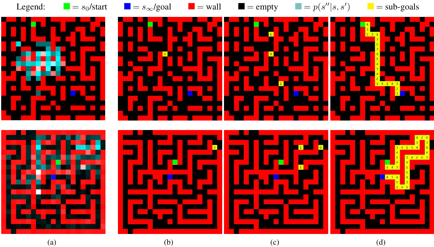
Figure 2. Grid-world maze examples for wall density $d=0.75$ (top row) and $d=0.95$ (bottom row). (a) The distribution over sub-goals induced by the policy prior $p$ that guides the DC-MCTS planner. (b)-(d) Visualization of the solution tree found by DC-MCTS: (b) The first sub-goal, i.e. at depth 0 of the solution tree. It approximately splits the problem in half. (c) The sub-goals at depth 1. Note there are two of them. (d) The final plan with the depth of each sub-goal shown. See supplementary material for animations.

图 2: 墙体密度 $d=0.75$ (上行) 和 $d=0.95$ (下行) 的网格世界迷宫示例。(a) 由指导 DC-MCTS 规划器的策略先验 $p$ 诱导的子目标分布。(b)-(d) DC-MCTS 找到的解树可视化：(b) 第一个子目标，即解树深度为 0 的节点。它近似将问题对半分割。(c) 深度为 1 的子目标。注意存在两个子目标。(d) 显示各子目标深度的最终规划方案。动画请参阅补充材料。

the optimal plan.

最优方案。

The proposed DC-MCTS planner is a MCTS (Browne et al., 2012) variant, that is inspired by recent advances in best-first or guided search, such as AlphaZero (Silver et al., 2018). It can also be understood as a heuristic, guided version of the classic Floyd-Warshall algorithm. The latter iterates over all sub-goals and then, in an inner loop, over all paths to and from a given sub-goal, for exhaustively computing all shortest paths. In the special case of planar graphs, small sub-goal sets, also known as vertex separators, can be constructed that favourably partition the remaining graph, leading to linear time ASAP algorithms (Henzinger et al., 1997). The heuristic sub-goal proposer $p$ that guides DCMCTS can be loosely understood as a probabilistic version of a vertex separator. Nowak-Vila et al. (2016) also consider neural networks that mimic divide-and-conquer algorithms similar to the sub-goal proposals used here. However, while we do policy improvement for the proposals using search and HER, the networks in (Nowak-Vila et al., 2016) are purely trained by policy gradient methods.

提出的DC-MCTS规划器是MCTS (Browne等人，2012) 的变体，其灵感来源于最佳优先或引导搜索领域的最新进展，例如AlphaZero (Silver等人，2018) 。它也可以被理解为经典Floyd-Warshall算法的启发式引导版本。后者会遍历所有子目标，然后在内部循环中遍历与给定子目标相关的所有路径，以穷举计算所有最短路径。在平面图的特殊情况下，可以构建小子目标集（也称为顶点分隔符）来有利地分割剩余图，从而产生线性时间的ASAP算法 (Henzinger等人，1997) 。引导DCMCTS的启发式子目标提议器$p$可以粗略地理解为顶点分隔符的概率版本。Nowak-Vila等人 (2016) 也考虑了模仿分治算法的神经网络，类似于本文使用的子目标提议。然而，虽然我们使用搜索和HER对提议进行策略改进，但 (Nowak-Vila等人，2016) 中的网络仅通过策略梯度方法进行训练。

Decomposing tasks into sub-problems has been formalized as pseudo trees (Freuder & Quinn, 1985) and AND/OR graphs (Nilsson, N. J., 1980). The latter have been used especially in the context of optimization (Larrosa et al.,

将任务分解为子问题已被形式化为伪树 (Freuder & Quinn, 1985) 和与或图 (Nilsson, N. J., 1980)。后者尤其被用于优化问题的场景 (Larrosa et al.,

2002; Jégou & Terrioux, 2003; Dechter & Mateescu, 2004; Marinescu & Dechter, 2004). Our approach is related to work on using AND/OR trees for sub-goal ordering in the context of logic inference (Ledeniov & Markovitch, 1998). While DC-MCTS is closely related to the $A O^{ * }$ algorithm (Nilsson, N. J., 1980), which is the generalization of the heuristic $A^{ * }$ search to AND/OR search graphs, interesting differences exist: $A O^{*}$ assumes a fixed search heuristic, which is required to be lower bound on the cost-to-go. In contrast, we employ learned value functions and policy priors that are not required to be exact bounds. Relaxing this assumption, thereby violating the principle of “optimism in the face of uncertainty”, necessitates explicit exploration incentives in the SELECT method. Alternatives for searching AND/OR spaces include proof-number search, which has recently been successfully applied to chemical synthesis planning (Kishimoto et al., 2019).

2002; Jégou & Terrioux, 2003; Dechter & Mateescu, 2004; Marinescu & Dechter, 2004)。我们的方法与逻辑推理中子目标排序的AND/OR树应用研究相关(Ledeniov & Markovitch, 1998)。虽然DC-MCTS与$AO^{ * }$算法(Nilsson, N. J., 1980)——即启发式$A^{ * }$搜索在AND/OR搜索图上的泛化形式——存在紧密联系，但存在有趣的差异：$AO^{*}$假定固定的搜索启发函数需满足剩余代价下界要求，而我们采用的学习价值函数和策略先验无需严格满足边界条件。放宽该假设会违反"不确定性下的乐观原则"，因此需要在SELECT方法中显式引入探索激励。AND/OR空间搜索的替代方案包括证明数搜索，该方法近期已成功应用于化学合成规划(Kishimoto et al., 2019)。

5. Experiments

5. 实验

We evaluate the proposed DC-MCTS algorithm on navigation in grid-world mazes as well as on a challenging continuous control version of the same problem. In our experiments, we compared DC-MCTS to standard sequential MCTS (in sub-goal space) based on the fraction of “solved” mazes by executing their plans. The MCTS baseline was implemented by restricting the DC-MCTS algorithm to only expand the “right” sub-problem in line 11 of Algorithm 1; all remaining parameters and design choice were the same for both planners except where explicitly mentioned otherwise. Videos of results can be found at https://sites.google.com/view/dc-mcts/home.

我们在网格世界迷宫导航以及该问题的连续控制挑战版本上评估了提出的DC-MCTS算法。实验中，我们通过执行规划方案解决迷宫的比例，将DC-MCTS与基于子目标空间的标准顺序MCTS进行对比。MCTS基线实现方式是将DC-MCTS算法限制为仅扩展算法1第11行的"右侧"子问题；除非另有明确说明，两个规划器的其余参数和设计选择均保持一致。结果视频可在 https://sites.google.com/view/dc-mcts/home 查看。

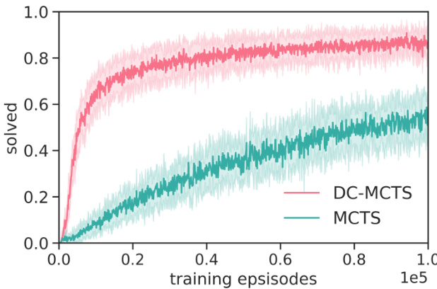
Figure 3. Performance of DC-MCTS and standard MCTS on gridworld maze navigation. Each episode corresponds to a new maze with wall density $d=0.75$ . Curves are averages and standard deviations over 20 different hyper parameters.

图 3: DC-MCTS与标准MCTS在网格世界迷宫导航中的性能对比。每个回合对应一个墙体密度 $d=0.75$ 的新迷宫。曲线为20组不同超参数下的平均值及标准差。

5.1. Grid-World Mazes

5.1. 网格世界迷宫

In this domain, each task consists of a new, procedurally generated maze on a $21\times21$ grid with start and goal locations $\left(s_{0},s_{\infty}\right)\in{1,\ldots,21}^{2}$ , see Figure 2. Task difficulty was controlled by the density of walls $d$ (under connected ness constraint), where the easiest setting $d=0.0$ corresponds to no walls and the most difficult one $d=1.0$ implies so-called perfect or singly-connected mazes. The task embedding $c_{\mathcal{M}}$ was given as the maze layout and $(s_{0},s_{\infty})$ encoded together as a feature map of $21\times21$ categorical variables with 4 categories each (empty, wall, start and goal location). The underlying MDPs have 5 primitive actions: up, down, left, right and NOOP. For sake of simplicity, we first tested our proposed approach by hard-coding a low-level policy $\pi^{0}$ as well as its value oracle $\boldsymbol{v}^{\pi^{0}}$ in the following way. If in state $s$ and conditioned on a goal $s^{\prime}$ , and if $s$ is adjacent to $s^{\prime}$ , $\pi_{s^{\prime}}^{0}$ successfully reaches $s^{\prime}$ with probability 1 in one step, i.e. $\begin{array}{r}{v^{\pi^{0}}(s,s^{\prime})=1}\end{array}$ ; otherwise $\begin{array}{r}{v^{\pi^{0}}(s,s^{\prime})=0}\end{array}$ . If $\pi_{s^{\prime}}^{0}$ is nevertheless executed, the agent moves to a random empty tile adjacent to $s$ . Therefore, $\pi^{0}$ is the “most myopic” goaldirected policy that can still navigate everywhere.

在该领域中，每个任务由程序化生成的 $21\times21$ 网格迷宫构成，包含起点和终点位置 $\left(s_{0},s_{\infty}\right)\in{1,\ldots,21}^{2}$ (见图2)。任务难度通过墙体密度 $d$ (在连通性约束下)控制，其中最简单设置 $d=0.0$ 对应无墙体，最困难设置 $d=1.0$ 对应所谓完美或单连通迷宫。任务嵌入 $c_{\mathcal{M}}$ 以迷宫布局和 $(s_{0},s_{\infty})$ 共同编码的形式给出，表示为 $21\times21$ 分类变量特征图，每个变量有4个类别(空地、墙体、起点和终点)。底层MDP包含5个基本动作：上、下、左、右和空操作(NOOP)。

为简化问题，我们首先通过硬编码低级策略 $\pi^{0}$ 及其值函数 $\boldsymbol{v}^{\pi^{0}}$ 来测试所提方法，具体实现如下：若在状态 $s$ 下以目标 $s^{\prime}$ 为条件，且 $s$ 与 $s^{\prime}$ 相邻时，策略 $\pi_{s^{\prime}}^{0}$ 能以概率1在一步内成功到达 $s^{\prime}$，即 $\begin{array}{r}{v^{\pi^{0}}(s,s^{\prime})=1}\end{array}$；否则 $\begin{array}{r}{v^{\pi^{0}}(s,s^{\prime})=0}\end{array}$。若仍执行 $\pi_{s^{\prime}}^{0}$，智能体会随机移动到与 $s$ 相邻的空地。因此，$\pi^{0}$ 是"最短视"但仍能全局导航的目标导向策略。

For each maze, MCTS and DC-MCTS were given a search budget of 200 calls to the low-level value oracle $\boldsymbol{v}^{\pi^{0}}$ . We implemented the search heuristics, i.e. policy prior $p$ and high-level value function $v$ , as convolutional neural networks which operate on input $c_{\mathcal{M}}$ ; details for the network architectures are given in Appendix B.3. With untrained networks, both planners were unable to solve the task $(<2%$ success probability), as shown in Figure 3. This illustrates that a search budget of 200 evaluations of $\boldsymbol{v}^{\pi^{0}}$ is insufficient for unguided planners to find a feasible path in most mazes. This is consistent with standard exhaustive SSSP / APSP graph planners requiring $21^{4}>10^{5}\gg200$ evaluations for optimal planning in the worst case on these tasks.

对于每个迷宫，MCTS和DC-MCTS的低级价值预言器$\boldsymbol{v}^{\pi^{0}}$的搜索预算设定为200次调用。我们将搜索启发式（即策略先验$p$和高级价值函数$v$）实现为卷积神经网络，其输入为$c_{\mathcal{M}}$；网络架构的详细信息见附录B.3。如图3所示，使用未经训练的网络时，两种规划器均无法完成任务（成功率<2%）。这表明，在大多数迷宫中，200次$\boldsymbol{v}^{\pi^{0}}$评估的搜索预算不足以让无引导的规划器找到可行路径。这与标准穷举SSSP/APSP图规划器在最坏情况下需要$21^{4}>10^{5}\gg200$次评估以实现最优规划的结果一致。

Next, we trained both search heuristics $v$ and $p$ as detailed in Section 3.2. In particular, the sub-goal proposal $p$ was also trained on hindsight-relabeled experience data, where for DC-MCTS we used the temporally balanced parser and for MCTS the corresponding left-first parser. Training of the heuristics greatly improved the performance of both planners. Figure 3 shows learning curves for mazes with wall density $d=0.75$ . DC-MCTS exhibits substantially improved performance compared to MCTS, and when compared at equal performance levels, DC-MCTS requires 5 to 10-times fewer training episodes than MCTS. The learned sub-goal proposal $p$ for DC-MCTS is visualized for two example tasks in Figure 2 (further examples are given in the Appendix in Figure 8). Probability mass concentrates on promising sub-goals that are far from both start and goal, approximately partitioning the task into equally hard subtasks.

接下来，我们按照第3.2节的详细说明训练了两种搜索启发式方法$v$和$p$。其中，子目标提议$p$的训练也使用了 hindsight-relabeled 经验数据：DC-MCTS采用时序平衡解析器，MCTS则使用对应的左优先解析器。启发式训练显著提升了两种规划器的性能。图3展示了墙体密度$d=0.75$迷宫的学习曲线。DC-MCTS相比MCTS展现出显著性能提升，在相同性能水平下，DC-MCTS所需的训练轮次比MCTS少5到10倍。图2展示了DC-MCTS学习到的子目标提议$p$在两个示例任务中的可视化效果（更多示例见附录图8），概率质量集中在远离起点和终点的潜力子目标上，这些子目标大致将任务划分为难度相当的子任务。

5.2. Continuous Control Mazes

5.2. 连续控制迷宫

Next, we investigated the performance of both MCTS and DC-MCTS in challenging continuous control environments with non-trivial low-level policies. To this end, we embedded the navigation in grid-world mazes described above into a physical 3D environment simulated by MuJoCo (Todorov et al., 2012), where each grid-world cell is rendered as $4\mathrm{m}\times4\mathrm{m}$ cell in physical space. The agent is embodied by a quadruped “ant” body; for illustration see Figure 4. For the low-level policy $\pi^{m}$ , we pre-trained a goal-directed neural network controller that gets as inputs proprio ce pti ve features (e.g. some joint angles and velocities) of the ant body as well as a 3D-vector pointing from its current position to a target position. $\pi^{m}$ was trained to navigate to targets randomly placed less than $1.5\mathrm{m~}$ away in an open area (no walls), using MPO (Abd ol malek i et al., 2018). See Appendix B.4 for more details. If unobstructed, $\pi^{m}$ can walk in a straight line towards its current goal. However, this policy receives no visual input and thus can only avoid walls when guided with appropriate sub-goals. In order to establish an interface between the low-level $\pi^{m}$ and the planners, we used another convolutional neural network to approximate the low-level value oracle $\boldsymbol{v}^{\pi^{m}}\left(s_{0},s_{\infty}|c_{\mathcal{M}}\right)$ : It was trained to predict whether $\pi^{m}$ will succeed in solving the navigation tasks $(s_{0},s_{\infty}),c_{\mathcal{M}}$ . Its input is given by the corresponding discrete grid-world representation $c_{\mathcal{M}}$ of the maze $(21\times21$ feature map of categorical s as described above, detail in Appendix). Note that this setting is still a difficult environment: In initial experiments we verified that a model-free baseline (also based on MPO) with access to state abstraction and low-level controller, only solved about $10%$ of the mazes after 100 million episodes due to the extremely sparse rewards.

接下来，我们研究了MCTS和DC-MCTS在具有复杂底层策略的连续控制环境中的性能。为此，我们将上述网格世界迷宫导航嵌入到由MuJoCo (Todorov et al., 2012) 模拟的物理3D环境中，其中每个网格单元在物理空间中呈现为$4\mathrm{m}\times4\mathrm{m}$的区域。智能体采用四足"蚂蚁"形态（示意图见图4）。对于底层策略$\pi^{m}$，我们预训练了一个目标导向的神经网络控制器，其输入包括蚂蚁本体的本体感知特征（如关节角度和速度）以及从当前位置指向目标位置的3D向量。$\pi^{m}$使用MPO (Abd ol malek i et al., 2018) 在开放区域（无墙体）训练导航至随机放置（距离小于$1.5\mathrm{m~}$）的目标点（详见附录B.4）。若无障碍，$\pi^{m}$可直线行进至当前目标，但由于缺乏视觉输入，该策略需依赖适当子目标引导才能避障。

为实现底层$\pi^{m}$与规划器的接口，我们采用另一个卷积神经网络来近似底层价值函数$\boldsymbol{v}^{\pi^{m}}\left(s_{0},s_{\infty}|c_{\mathcal{M}}\right)$：该网络被训练用于预测$\pi^{m}$能否成功完成导航任务$(s_{0},s_{\infty}),c_{\mathcal{M}}$，其输入为迷宫的离散网格表示$c_{\mathcal{M}}$（21×21分类特征图，详见附录）。需注意该环境仍具挑战性：初步实验表明，具备状态抽象和底层控制器访问权限的无模型基线（同样基于MPO）在1亿次训练后仅能解决约$10%$的迷宫，这归因于奖励极度稀疏的特性。

Figure 4. Navigation in a physical MuJoCo domain. The agent, situated in an "ant"-like body, should navigate to the green target.

图 4: 物理 MuJoCo 环境中的导航任务。智能体位于一个类似"蚂蚁"的身体中，需要导航至绿色目标位置。

We applied the MCTS and DC-MCTS planners to this problem to find symbolic plans consisting of sub-goals in ${1,\ldots,21}^{2}$ . The high-level heuristics $p$ and $v$ were trained for $65\mathrm{k\Omega}$ episodes, exactly as described in Section 5.1, except using $v^{\pi^{m}}$ instead of $\boldsymbol{v}^{\pi^{0}}$ . We again observed that DCMCTS outperforms by a wide margin the vanilla MCTS planner: Figure 5 shows performance of both (with fully trained search heuristics) as a function of the search budget for the most difficult mazes with wall density $d=1.0$ Performance of DC-MCTS with the MuJoCo low-level controller was comparable to that with the hard-coded low-level policy from the grid-world experiment (with same wall density), showing that the abstraction of planning over low-level sub-goals successfully isolates high-level planning from low-level execution. We did not manage to successfully train the MCTS planner on MuJoCo navigation. This was likely due to the fact that HER training, which we found — in ablation studies — essential for training DC-MCTS on both problem versions and MCTS on the grid-world problem, was not appropriate for MCTS on MuJoCo navigation: Left-first parsing for selecting sub-goals for HER training consistently biased the MCTS search prior $p$ to propose next sub-goals too close to the previous sub-goal. This lead the MCTS planner to "micro-manage" the low-level policy too much, in particular in long corridors that $\pi^{m}$ can solve by itself. DC-MCTS, by recursively partitioning, found an appropriate length scale of sub-goals, leading to drastically improved performance.

我们将MCTS和DC-MCTS规划器应用于此问题，以寻找由 ${1,\ldots,21}^{2}$ 中子目标组成的符号化计划。高层启发式 $p$ 和 $v$ 经过 $65\mathrm{k\Omega}$ 轮训练，具体如第5.1节所述，但使用 $v^{\pi^{m}}$ 而非 $\boldsymbol{v}^{\pi^{0}}$ 。我们再次观察到DC-MCTS显著优于普通MCTS规划器：图5展示了二者（使用完全训练的搜索启发式）在最具挑战性的迷宫（墙体密度 $d=1.0$）中随搜索预算变化的性能表现。DC-MCTS搭配MuJoCo底层控制器的性能与网格世界实验中硬编码底层策略（相同墙体密度）相当，表明基于底层子目标的规划抽象成功将高层规划与底层执行分离。我们未能成功在MuJoCo导航任务上训练MCTS规划器，这可能是因为——在消融研究中发现——对两个问题版本的DC-MCTS训练及网格世界问题的MCTS训练至关重要的HER训练，并不适用于MuJoCo导航的MCTS：为HER训练选择子目标的左优先解析持续使MCTS搜索先验 $p$ 倾向于提议距离前一个子目标过近的新子目标，导致MCTS规划器对底层策略"过度微观管理"，尤其在 $\pi^{m}$ 可独立解决的长走廊场景中。而DC-MCTS通过递归分区找到了合适的子目标长度尺度，从而大幅提升性能。

Visualizing MCTS and DC-MCTS To further illustrate the difference between DC-MCTS and MCTS planning we can look at an example search tree from each method in

可视化MCTS与DC-MCTS
为更直观展示DC-MCTS与MCTS规划的区别，我们可以观察两种方法生成的搜索树示例。

Figure 5. Performance of DC-MCTS and standard MCTS on continuous control maze navigation as a function of planning budget. Mazes have wall density $d=1.0$ . Shown is the outcome of the single best hyper-parameter run, confidence intervals are defined as one standard deviation of the corresponding multi no mi al computed over 100 mazes.

图 5: DC-MCTS与标准MCTS在连续控制迷宫导航任务中的性能对比(随规划预算变化)。迷宫墙体密度为$d=1.0$。展示结果为单组最优超参数运行的输出，置信区间定义为100个迷宫上计算的多项分布的一个标准差。

Figure 6. Light blue nodes are part of the final plan: note how in the case of DC-MCTS, the plan is distributed across a sub-tree within the search tree, while for the standard MCTS the plan is a single chain. The first ‘actionable’ sub-goal, i.e. the first sub-goal that can be passed to the low-level policy, is the left-most leaf in DC-MCTS and the first dark node from the root for MCTS.

图 6: 浅蓝色节点为最终计划组成部分。注意在DC-MCTS中，计划分布在搜索树的子树内，而标准MCTS的计划为单一链式结构。首个"可执行"子目标(即首个可传递给底层策略的子目标)，在DC-MCTS中是最左侧叶节点，在MCTS中则是从根节点算起的第一个深色节点。

6. Discussion

6. 讨论

To enable guided, divide-and-conquer style planning, we made a few strong assumptions. Sub-goal based planning requires a universal value function oracle of the low-level policy. In many applications, this will have to be approximated from data. Overly optimistic approximations are likely be exploited by the planner, leading to “delusional” plans (Little & Thiébaux, 2007). Joint learning of the high and low-level components can potentially address this issue. A further limitation of sub-goal planning is that, at least in its current naive implementation, the "action space" for the planner is the whole state space of the underlying MDPs. Therefore, the search space will have a large branching factor in large state spaces. A solution to this problem likely lies in using learned state abstractions for sub-goal specifications, which is a fundamental open research question. We also implicitly made the assumption that low-level skills afforded by the low-level policy need to be “universal”, i.e. if there are states that it cannot reach, no amount of high level search will lead to successful planning outcomes.

为实现分步引导式规划，我们做了几个强假设。基于子目标的规划需要底层策略具备通用价值函数预言机。在许多应用中，这需要通过数据近似实现。过于乐观的近似可能被规划器利用，导致出现"妄想型"计划 (Little & Thiébaux, 2007)。高低层组件的联合学习可能解决此问题。子目标规划的另一个局限是，至少在当前简单实现中，规划器的"动作空间"是底层MDP的整个状态空间，因此在大型状态空间中会产生高分支因子的搜索空间。该问题的解决方案可能在于使用学习到的状态抽象来指定子目标，这是基础性开放研究课题。我们还隐含假设底层策略提供的低级技能需具备"通用性"，即若存在无法到达的状态，任何高层搜索都无法产生成功规划结果。

In spite of these assumptions and open challenges, we showed that non-sequential sub-goal planning has some fundamental advantages over the standard approach of search over primitive actions: (i) Abstraction and dynamic allocation: Sub-goals automatically support temporal abstraction as the high-level planner does not need to specify the exact time horizon required to achieve a sub-goal. Plans are generated from coarse to fine, and additional planning is dynamically allocated to those parts of the plan that require more compute. (ii) Closed & open-loop: The approach combines advantages of both open- and closed loop planning: The closed-loop low-level policies can recover from failures or unexpected transitions in stochastic environments, while at the same time the high-level planner can avoid costly closed-loop planning. (iii) Long horizon credit assignment: Sub-goal abstractions open up new algorithmic possibilities for planning — as exemplified by DC-MCTS — that can facilitate credit assignment and therefore reduce planning complexity. (iv) Parallel iz ation: Like other divide-and-conquer algorithms, DC-MCTS lends itself to parallel execution by leveraging problem decomposition made explicit by the independence of the "left" and "right" sub-problems of an AND node. (v) Reuse of cached search: DC-MCTS is highly amenable to transposition tables, by caching and reusing values for sub-problems solved in other branches of the search tree. (vi) Generality: DC-MCTS is strictly more general than both forward and backward goal-directed planning, both of which can be seen as special cases.

尽管存在这些假设和开放挑战，我们证明了非顺序子目标规划相比基于原始动作的标准搜索方法具有以下根本优势：(i) 抽象与动态分配：子目标自动支持时间抽象，高层规划器无需指定实现子目标的确切时间跨度。规划过程由粗到细生成，系统会动态分配额外计算资源给需要更复杂处理的规划部分。(ii) 闭环与开环结合：该方法融合了开环与闭环规划的双重优势：闭环底层策略能从随机环境中的失败或意外状态中恢复，同时高层规划器可避免昂贵的闭环规划开销。(iii) 长周期信用分配：子目标抽象为规划算法（如DC-MCTS所示范）开辟了新可能性，能促进信用分配从而降低规划复杂度。(iv) 并行化：与其他分治算法类似，DC-MCTS通过利用AND节点"左""右"子问题的独立性实现显式问题分解，天然适合并行执行。(v) 缓存搜索复用：DC-MCTS高度适配置换表机制，通过缓存和复用搜索树其他分支已解决的子问题估值。(vi) 通用性：DC-MCTS严格涵盖了前向与后向目标导向规划，两者均可视为其特例。

Figure 6. On the left the search tree for DC-MCTS, on the right for regular MCTS. Only colored nodes are part of the final plan. Note that for MCTS the final plan is a chain, while for DC-MCTS it is a sub-tree.

图 6: 左侧为DC-MCTS的搜索树，右侧为常规MCTS。仅着色节点属于最终规划方案。注意MCTS的最终方案呈链式结构，而DC-MCTS的最终方案为子树结构。

Acknowledgments

致谢

The authors wish to thank Benigno Uría, David Silver, Loic Matthey, Niki Kilbertus, Alessandro Ialongo, Pol Moreno, Steph Hughes-Fitt, Charles Blundell and Daan Wierstra for helpful discussions and support in the preparation of this work.

作者谨此感谢Benigno Uría、David Silver、Loic Matthey、Niki Kilbertus、Alessandro Ialongo、Pol Moreno、Steph Hughes-Fitt、Charles Blundell和Daan Wierstra在本研究筹备过程中提供的宝贵讨论与支持。

References

参考文献

Abd ol malek i, A., Spring e nberg, J. T., Tassa, Y., Munos, R., Heess, N., and Riedmiller, M. Maximum a posteriori policy optimisation. In International Conference on Learning Representations, 2018.

Abd ol malek i, A., Spring e nberg, J. T., Tassa, Y., Munos, R., Heess, N., and Riedmiller, M. 最大后验策略优化。In International Conference on Learning Representations, 2018.

An dry ch owicz, M., Wolski, F., Ray, A., Schneider, J., Fong, R., Welinder, P., McGrew, B., Tobin, J., Pieter Abbeel, O., and Zaremba, W. Hindsight Experience Replay. In Guyon, I., Luxburg, U. V., Bengio, S., Wallach, H., Fer- gus, R., Vishwanath an, S., and Garnett, R. (eds.), Ad

Proceedings of the 34th International Conference on Machine Learning-Volume 70, pp. 3540–3549. JMLR. org, 2017.

第34届国际机器学习大会论文集-第70卷，第3540–3549页。JMLR.org，2017年。

Zhang, A., Lerer, A., Sukhbaatar, S., Fergus, R., and Szlam, A. Composable planning with attributes. arXiv preprint arXiv:1803.00512, 2018.

Zhang, A., Lerer, A., Sukhbaatar, S., Fergus, R., and Szlam, A. 基于属性的可组合规划。arXiv预印本 arXiv:1803.00512, 2018。

A. Additional Details for DC-MCTS

A. DC-MCTS 的附加细节

A.1. Proof of Proposition 1

A.1. 命题1的证明

Proof. The performance of $\pi_{\sigma}$ on the task $(s_{0},s_{\infty})$ is defined as the probability that its trajectory $\tau_{s_{0}}^{\pi_{\sigma}}$ from initial state $s_{0}$ gets absorbed in the state $s_{\infty}$ , i.e. $P(s_{\infty}\in\tau_{s_{0}}^{\pi_{\sigma}})$ . We can bound the latter from below in the following way. Let $\sigma=(\sigma_{0},\ldots,\sigma_{m})$ , with $\sigma_{0}=s_{0}$ and $\sigma_{m}=s_{\infty}$ . With $(\sigma_{0},\ldots,\sigma_{i})\subseteq\tau_{s_{0}}^{\pi_{\sigma}}$ we denote the event that $\pi_{\sigma}$ visits all states $\sigma_{0},\ldots,\sigma_{i}$ in order:

证明。策略 $\pi_{\sigma}$ 在任务 $(s_{0},s_{\infty})$ 上的性能定义为：从初始状态 $s_{0}$ 出发的轨迹 $\tau_{s_{0}}^{\pi_{\sigma}}$ 被吸收到状态 $s_{\infty}$ 的概率，即 $P(s_{\infty}\in\tau_{s_{0}}^{\pi_{\sigma}})$ 。我们可以通过以下方式给出该概率的下界。设 $\sigma=(\sigma_{0},\ldots,\sigma_{m})$ ，其中 $\sigma_{0}=s_{0}$ 且 $\sigma_{m}=s_{\infty}$ 。用 $(\sigma_{0},\ldots,\sigma_{i})\subseteq\tau_{s_{0}}^{\pi_{\sigma}}$ 表示事件：策略 $\pi_{\sigma}$ 按顺序访问所有状态 $\sigma_{0},\ldots,\sigma_{i}$ 。

$$
P((\sigma_{0},\dots,\sigma_{i})\subseteq\tau_{s_{0}}^{\pi_{\sigma}})=P\left(\bigwedge_{i^{\prime}=1}^{i}(\sigma_{i^{\prime}}\in\tau_{s_{0}}^{\pi_{\sigma}})\wedge(t_{i^{\prime}-1}<t_{i^{\prime}})\right),
$$

where $t_{i}$ is the arrival time of $\pi_{\sigma}$ at $\sigma_{i}$ , and we define $t_{0}=0$ . Obviously, the event $\left(\sigma_{0},\ldots,\sigma_{m}\right)\subseteq\tau_{s_{0}}^{\pi_{\sigma}}$ is a subset of the event $s_{\infty}\in\tau_{s_{0}}^{\pi_{\sigma}}$ , and therefore

其中 $t_{i}$ 是 $\pi_{\sigma}$ 到达 $\sigma_{i}$ 的时间，我们定义 $t_{0}=0$。显然，事件 $\left(\sigma_{0},\ldots,\sigma_{m}\right)\subseteq\tau_{s_{0}}^{\pi_{\sigma}}$ 是事件 $s_{\infty}\in\tau_{s_{0}}^{\pi_{\sigma}}$ 的子集，因此

$$
P((\sigma_{0},\dots,\sigma_{m})\subseteq\tau_{s_{0}}^{\pi_{\sigma}})\leq P(s_{\infty}\in\tau_{s_{0}}^{\pi_{\sigma}}).
$$

Using the chain rule of probability we can write the lhs as:

利用概率的链式法则，我们可以将左侧表示为：

$$
P((\sigma_{0},\ldots,\sigma_{m})\subseteq\tau_{s_{0}}^{\pi_{\sigma}})=\prod_{i=1}^{m}P\left((\sigma_{i}\in\tau_{s_{0}}^{\pi_{\sigma}})\land(t_{i-1}<t_{i})\mid(\sigma_{0},\ldots,\sigma_{i-i})\subseteq\tau_{s_{0}}^{\pi_{\sigma}}\right).
$$

We now use the definition of $\pi_{\sigma}\colon A f t e r$ reaching $\sigma_{i-1}$ and before reaching $\sigma_{i},\pi_{\sigma}$ is defined by just executing $\pi_{\sigma_{i}}$ starting from the state σi−1:

我们现在使用 $\pi_{\sigma}\colon A f t e r$ 的定义：在到达 $\sigma_{i-1}$ 之后且未到达 $\sigma_{i}$ 之前，$\pi_{\sigma}$ 仅定义为从状态 $\sigma_{i-1}$ 开始执行 $\pi_{\sigma_{i}}$。

$$
P((\sigma_{0},\ldots,\sigma_{m})\subseteq\tau_{s_{0}}^{\pi_{\sigma}})=\prod_{i=1}^{m}P\left(\sigma_{i}\in\tau_{\sigma_{i-1}}^{\pi_{\sigma_{i}}}\mid(\sigma_{0},\ldots,\sigma_{i-i})\subseteq\tau_{s_{0}}^{\pi_{\sigma}}\right).
$$

We now make use of the fact that the $\sigma_{i}\in S$ are states of the underlying MDP that make the future independent from the past: Having reached $\sigma_{i-1}$ at $t_{i-1}$ , all events from there on (e.g. reaching $\sigma_{j}$ for $j\geq i$ ) are independent from all event before $t_{i-1}$ . We can therefore write:

我们现在利用$\sigma_{i}\in S$是底层MDP状态这一事实，使得未来与过去独立：在$t_{i-1}$时刻到达$\sigma_{i-1}$后，之后的所有事件（例如在$j\geq i$时到达$\sigma_{j}$）都与$t_{i-1}$之前的所有事件无关。因此可以写成：

$$
\begin{array}{r c l}{{\displaystyle{\cal P}((\sigma_{0},\dots,\sigma_{m})\subseteq\tau_{s_{0}}^{\pi_{\sigma}})}}&{{=}}&{{\displaystyle\prod_{i=1}^{m}{\cal P}\left(\sigma_{i}\in\tau_{\sigma_{i-1}}^{\pi_{\sigma_{i}}}\right)}}\ {{}}&{{=}}&{{\displaystyle\prod_{i=1}^{m}v^{\pi}\left(\sigma_{i-1},\sigma_{i}\right).}}\end{array}
$$

Putting together equation 3 and equation 4 yields the proposition.

将方程3和方程4联立可得该命题。

A.2. Additional algorithmic details

A.2. 额外算法细节

After the search phase, in which DC-MCTS builds the search tree $\tau$ , it returns its estimate of the best plan $\hat{\sigma}^{ * }$ and the corresponding lower bound $L(\hat{\sigma}^{*})$ by calling the EXTRACT PLAN procedure on the root node $(s_{0},s_{\infty})$ . Algorithm 2 gives details on this procedure.

在搜索阶段，DC-MCTS构建搜索树$\tau$后，通过对根节点$(s_{0},s_{\infty})$调用EXTRACT PLAN过程，返回其对最佳计划$\hat{\sigma}^{ * }$的估计以及相应的下限$L(\hat{\sigma}^{*})$。算法2详细描述了这一过程。

A.3. Descending into one node at the time during search

A.3. 搜索时每次下降一个节点

Instead of descending into both nodes during the TRAVERSE step of Algorithm 1, it is possible to choose only one of the two sub-problems to expand further. This can be especially useful if parallel computation is not an option, or if there are specific needs e.g. as illustrated by the following three heuristics. These can be used to decide when to traverse into the left sub-problem $(s,s^{\prime})$ or the right sub-problem $(s^{\prime},s^{\prime\prime})$ . Note that both nodes have a corresponding current estimate for their value $V$ , coming either from the bootstrap evaluation of $v$ or further refined from previous traversals.

在算法1的TRAVERSE步骤中，可以选择仅扩展两个子问题中的一个而非同时深入两个节点。这在无法进行并行计算或存在特定需求时尤为实用，例如以下三种启发式方法所示。这些方法可用于决定何时深入左子问题$(s,s^{\prime})$或右子问题$(s^{\prime},s^{\prime\prime})$。需注意，两个节点都有对应的当前价值估计值$V$，该值可能来自$v$的引导评估，也可能通过先前遍历得到进一步优化。

Figure 7. Divide and Conquer Tree Search is strictly more general than both forward and backward search.

图 7: 分治树搜索 (Divide and Conquer Tree Search) 严格优于前向搜索和后向搜索。

Algorithm 2 additional Divide-And-Conquer MCTS procedures
Globallow-levelvalueoraclevm Global high-level value function v
	Global policy prior p
	GlobalsearchtreeT
1: procedure EXTRACTPLAN(OR node (s, s")) s' ← arg maxs V(s,s) · V(s, s") choose best sub-goal no more splitting 6: O1,G EXTRACTPLAN(s, S') extract "left" sub-plan 7: Or, Gr EXTRACTPLAN(s', s") > extract "right" sub-plan
2: 3: if s =then 4: return O, v"(s, s") 5: else

算法 2 附加的分治蒙特卡洛树搜索流程
全局低层价值预言机 vm 全局高层价值函数 v
全局策略先验 p
全局搜索树 T
1: 过程 EXTRACTPLAN(或节点 (s, s"))
s' ← arg maxs V(s,s) · V(s, s") 选择最佳子目标
不再分裂
6: O1,G EXTRACTPLAN(s, S') 提取"左"子计划
7: Or, Gr EXTRACTPLAN(s', s") 提取"右"子计划
2: 3: 如果 s = 则
4: 返回 O, v"(s, s")
5: 否则

• Preferentially descend into the left node encourages a more accurate evaluation of the near future, which is more relevant to the current choices of the agent. This makes sense when the right node can be further examined later, or there is uncertainty about the future that makes it sub-optimal to design a detailed plan at the moment. • Preferentially descend into the node with a lower value, following the principle that a chain (plan) is only as good as its weakest link (sub-problem). This heuristic effectively greedily optimizes for the overall value of the plan. • Use 2-way UCT on the values of the nodes, which acts similarly to the previous greedy heuristic, but also takes into account the confidence over the value estimates given by the visit counts.

• 优先深入左节点能更准确地评估近期未来，这与智能体当前的选择更为相关。当右节点可以在后续检查时，或存在未来不确定性使得当前制定详细计划并非最优时，这种做法是合理的。
• 遵循"链条（计划）的强度取决于其最薄弱环节（子问题）"的原则，优先深入值较低的节点。这种启发式方法有效地以贪婪方式优化计划的整体价值。
• 对节点值使用双向UCT (Upper Confidence Bound for Trees)，其作用类似于先前的贪婪启发式方法，但还会考虑访问计数给出的价值估计置信度。

The rest of the algorithm can remain unchanged, and during the BACKUP phase the current value estimate $V$ of the sibling sub-problem can be used.

算法的其余部分可以保持不变，在 BACKUP 阶段可以使用兄弟子问题的当前值估计 $V$。

B. Training details

B. 训练细节

B.1. Details for training the value function

B.1. 价值函数训练细节

In order to train the value network $v$ , that is used for boots trapping in DC-MCTS, we can regress it towards targets computed from previous search results or environment experiences. A first obvious option is to use as regression target the Monte Carlo return (i.e. 0 if the goal was reached, and 1 if it was not) from executing the DC-MCTS plans in the environment. This appears to be a sensible target, as the return is an unbiased estimator of the success probability $P(s_{\infty}\in\tau_{s_{0}}^{\pi_{\sigma}})$ of the plan. Although this approach was used in (Silver et al., 2016), its downside is that gathering environment experience is often very costly and only yields little information, i.e. one binary variable per episode. Furthermore no other information from the generated search tree $\tau$ except for the best plan is used. Therefore, a lot of valuable information might be discarded, in particular in situations where a good sub-plan for a particular sub-problem was found, but the overall plan nevertheless failed.

为了训练用于DC-MCTS中自举(bootstrapping)的价值网络$v$，我们可以将其回归到基于先前搜索结果或环境经验计算的目标值。最直观的方案是使用在环境中执行DC-MCTS计划获得的蒙特卡洛回报（即达成目标时为0，未达成时为1）作为回归目标。这看似合理的方案是因为该回报是计划成功概率$P(s_{\infty}\in\tau_{s_{0}}^{\pi_{\sigma}})$的无偏估计量。虽然(Silver et al., 2016)采用了这种方法，但其缺陷在于获取环境经验的成本通常极高且信息量极少（即每个回合仅产生一个二元变量）。此外，除最优计划外，生成的搜索树$\tau$中的其他信息均未被利用。因此大量有价值的信息可能被丢弃，特别是在已找到特定子问题的优质子计划、但整体计划仍失败的情况下。

This shortcoming could be remedied by using as regression targets the non-parametric value estimates $V(s,s^{\prime\prime})$ for all OR nodes $(s,s^{\prime\prime})$ in the DC-MCTS tree at the end of the search. With this approach, a learning signal could still be obtained from successful sub-plans of an overall failed plan. However, we empirically found in our experiments that this lead to drastically over-optimistic value estimates, for the following reason. By standard policy improvement arguments, regressing toward $V$ leads to a bootstrap value function that converges to $v^{ * }$ . In the definition of the optimal value $\begin{array}{r}{v^{\ast}(s,s^{\prime\prime})=\operatorname*{max}_{s^{\prime}}v^{\ast}(s,s^{\prime})\cdot v^{\ast}(s^{\prime},s^{\prime\prime})}\end{array}$ , we implicitly allow for infinite recursion depth for solving sub-problems. However, in practice, we often used quite shallow trees (depth $<10$ ), so that boots trapping with approximations of $v^{*}$ is too optimistic, as this assumes unbounded planning budget. A principled solution for this could be to condition the value function for boots trapping on the amount of remaining search budget, either in terms of remaining tree depth or node expansions.

这一缺陷可以通过使用搜索结束时DC-MCTS树中所有OR节点$(s,s^{\prime\prime})$的非参数化价值估计$V(s,s^{\prime\prime})$作为回归目标来弥补。这种方法仍能从整体失败计划的成功子计划中获取学习信号。但实验发现，这种做法会导致价值估计严重过度乐观，原因如下：根据标准策略改进理论，向$V$回归会得到一个收敛于$v^{ * }$的自举价值函数。在最优价值$\begin{array}{r}{v^{\ast}(s,s^{\prime\prime})=\operatorname*{max}_{s^{\prime}}v^{\ast}(s,s^{\prime})\cdot v^{\ast}(s^{\prime},s^{\prime\prime})}\end{array}$的定义中，我们隐式允许无限递归深度来解决子问题。然而实践中常使用较浅的树（深度$<10$），因此用$v^{*}$近似值进行自举过于乐观，因为这假设了无限的规划预算。一个理论解决方案是将自举价值函数与剩余搜索预算（剩余树深度或节点扩展次数）相关联。

Instead of the cumbersome, explicitly resource-aware value function, we found the following to work well. After planning with DC-MCTS, we extract the plan $\hat{\sigma}^{ * }$ with EXTRACT PLAN from the search tree $\tau$ . As can be seen from Algorithm 2, the procedure computes the return $G_{\hat{\sigma}^{ * }}$ for all OR nodes in the solution tree $\boldsymbol{\mathcal{T}}_ {\hat{\sigma}^{ * }}$ . For training $v$ we chose these returns $G_{\hat{\sigma}^{*}}$ for all OR nodes in the solution tree as regression targets. This combines the favourable aspects of both methods described above. In particular, this value estimate contains no boots trapping and therefore did not lead to overly-optimistic bootstraps. Furthermore, all successfully solved sub-problems given a learning signal. As regression loss we chose cross-entropy.

我们发现以下方法效果良好，避免了繁琐且显式资源感知的价值函数。在使用DC-MCTS规划后，我们通过EXTRACT PLAN从搜索树$\tau$中提取计划$\hat{\sigma}^{ * }$。如算法2所示，该过程为解树$\boldsymbol{\mathcal{T}}_ {\hat{\sigma}^{ * }}$中的所有OR节点计算收益$G_{\hat{\sigma}^{ * }}$。在训练$v$时，我们选择解树中所有OR节点的这些收益$G_{\hat{\sigma}^{*}}$作为回归目标。这结合了上述两种方法的优势：该价值估计不含自助法(bootstrapping)，因此不会产生过度乐观的自助结果；同时所有成功解决的子问题都能提供学习信号。我们选用交叉熵作为回归损失函数。

B.2. Details for training the policy prior

B.2. 策略先验训练的详细说明

The prior network is trained to match the distribution of the values of the AND nodes, also with a cross-entropy loss. Note that we did not use visit counts as targets for the prior network — as done in AlphaGo and AlphaZero for example (Silver et al., 2016; 2018)— since for small search budgets visit counts tend to be noisy and require significant fine-tuning to avoid collapse (Hamrick et al., 2020).

先验网络通过交叉熵损失训练，以匹配AND节点值的分布。需要注意的是，我们没有像AlphaGo和AlphaZero那样(Silver et al., 2016; 2018)将访问计数作为先验网络的目标，因为在较小搜索预算下，访问计数往往存在噪声，且需要大量微调以避免崩溃(Hamrick et al., 2020)。

B.3. Neural networks architectures for grid-world experiments

B.3. 网格世界实验的神经网络架构

The shared torso of the prior and value network used in the experiments is a 6-layer CNN with kernels of size 3, 64 filters per layer, Layer Normalization after every convolutional layer, swish (cit) as activation function, zero-padding of 1, and strides [1, 1, 2, 1, 1, 2] to increase the size of the receptive field.

实验中先验网络和价值网络共用的主干结构是一个6层CNN，每层使用大小为3的卷积核、64个滤波器，每层卷积后接层归一化(Layer Normalization)，激活函数采用swish [cit]，零填充为1，步长设置为[1, 1, 2, 1, 1, 2]以增大感受野范围。

The two heads for the prior and value networks follow the pattern described above, but with three layers only instead of six, and fixed strides of 1. The prior head ends with a linear layer and a softmax, in order to obtain a distribution over sub-goals. The value head ends with a linear layer and a sigmoid that predicts a single value, i.e. the probability of reaching the goal from the start state if we further split the problem into sub-problems.

先验网络和价值网络的两个头部遵循上述模式，但仅有三层而非六层，且固定步长为1。先验头部以线性层和softmax结尾，以获得子目标的分布。价值头部以线性层和sigmoid结尾，预测单个值（即若将问题进一步拆分为子问题，从初始状态到达目标的概率）。

We did not heavily optimize networks hyper-parameters. After running a random search over hyper-parameters for the fixed architecture described above, the following were chosen to run the experiments in Figure 3. The replay buffer has a maximum size of 2048. The prior and value networks are trained on batches of size 128 as new experiences are collected. Networks are trained using Adam with a learning rate of 1e-3, the boltzmann temperature of the softmax for the prior network set to 0.003. For simplicity, we used HER with the time-based rebalancing (i.e. turning experiences into temporal binary search trees). UCB constants are sampled uniformly between 3 and 7, as these values were observed to give more robust results.

我们没有对网络超参数进行过多优化。在针对上述固定架构进行超参数随机搜索后，选定以下配置运行图3中的实验：回放缓冲区最大容量为2048，先验网络和价值网络采用128的批量大小进行训练（随新经验收集动态更新）。网络训练使用学习率为1e-3的Adam优化器，先验网络的softmax玻尔兹曼温度设为0.003。为简化实现，我们采用基于时间重平衡的HER方法（即将经验转化为时序二叉搜索树）。UCB常数在3到7之间均匀采样，实验观测表明该区间能产生更稳定的结果。

B.4. Low-level controller training details

B.4. 底层控制器训练细节

For physics-based experiments using MuJoCo (Todorov et al., 2012), we trained a low-level policy first and then trained the planning agent to reuse the low-level motor skills afforded by this body and pretrained policy. The low-level policy, was trained to control the quadruped (“ant”) body to go to a randomly placed target in an open area (a “go-to-target” task, essentially the same as the task used to train the humanoid in Merel et al., 2019, which is available at dm_control/locomotion). The task amounts to the environment providing an instruction corresponding to a target position that the agent is is rewarded for moving to (i.e, a sparse reward when within a region of the target). When the target is obtained, a new target is generated that is a short distance away $(<1.5\mathrm{m})$ . What this means is that a policy trained on this task should be capable of producing short, direct, goal-directed locomotion behaviors in an open field. And at test time, the presence of obstacles will catastrophically confuse the trained low-level policy. The policy architecture, consisting of a shallow MLP for the actor and critic, was trained to solve this task using MPO (Abd ol malek i et al., 2018). More specifically, the actor and critic had respectively 2 and 3 hidden layers, 256 units each and elu activation function. The policy was trained to a high level of performance using a distributed, replay-based, off-policy training setup involving 64 actors. In order to reuse the low-level policy in the context of mazes, we can replace the environment-provided instruction with a message sent by a high-level policy (i.e., the planning agent). For the planning agent that interfaces with the low-level policy, the action space of the high-level policy will, by construction, correspond to the instruction to the low-level policy.

对于使用MuJoCo (Todorov等人, 2012) 的物理实验，我们首先训练了一个低级策略，然后训练规划智能体来复用该身体和预训练策略提供的低级运动技能。该低级策略被训练用于控制四足("ant")身体在开放区域移动到随机放置的目标(即"前往目标"任务，本质上与Merel等人2019年用于训练人形机器人的任务相同，该任务可在dm_control/locomotion获取)。该任务相当于环境提供一个对应于目标位置的指令，智能体因移动到该位置而获得奖励(即当处于目标区域时获得稀疏奖励)。当获得目标后，会在短距离内 $(<1.5\mathrm{m})$ 生成一个新目标。这意味着在该任务上训练的策略应能在开放场地中产生简短、直接、目标导向的运动行为。而在测试时，障碍物的存在会使训练好的低级策略严重混乱。该策略架构由用于行动器和评价器的浅层MLP组成，使用MPO (Abd ol malek i等人, 2018)训练以解决此任务。更具体地说，行动器和评价器分别具有2层和3层隐藏层，每层256个单元，使用elu激活函数。该策略通过涉及64个行动器的分布式、基于经验回放的离策略训练设置训练至高性能水平。为了在迷宫环境中复用低级策略，我们可以用高级策略(即规划智能体)发送的消息替换环境提供的指令。对于与低级策略交互的规划智能体，高级策略的动作空间在构造上将对应于对低级策略的指令。

B.5. Pseudocode

B.5. 伪代码

We summarize the training procudre for DC-MCTS in the following pseudo-code.

我们通过以下伪代码总结了DC-MCTS的训练流程。

Table 1. Architectures of the neural networks used in the experiment section for the high-level value and prior. For each convolutional layer we report kernel size, number of filters and stride. LN stands for Layer normalization, FC for fully connected,. All convolutions are preceded by a 1 pixel zero padding.

表1: 实验部分使用的高层价值网络与先验网络的神经网络架构。每个卷积层均标注了核尺寸、滤波器数量和步长。LN表示层归一化 (Layer normalization)，FC表示全连接层 (fully connected)。所有卷积操作前均进行1像素零填充。

Valuehead

3 × 3, 64, stride = 1

swish, LN

3 × 3,64, stride = 1

swish, LN

3 × 3, 64, stride = 1

swish, LN

Flatten

FC: Nh = 1

sigmoid

Valuehead
3 × 3, 64, 步长 = 1
swish, LN
3 × 3, 64, 步长 = 1
swish, LN
3 × 3, 64, 步长 = 1
swish, LN
Flatten
FC: Nh = 1
sigmoid

Torso

3 × 3,64, stride = 1

swish, LN

3 × 3, 64, stride = 1

swish, LN

3 × 3, 64, stride = 2

swish, LN

3 × 3, 64, stride = 1

swish, LN

3 × 3, 64, stride = 1

swish, LN

3 × 3,64, stride = 2

swish, LN

躯干部分
3×3,64, 步长=1
swish, LN
3×3,64, 步长=1
swish, LN
3×3,64, 步长=2
swish, LN
3×3,64, 步长=1
swish, LN
3×3,64, 步长=1
swish, LN
3×3,64, 步长=2
swish, LN

Policy head

3 × 3,64, stride = 1

swish, LN

3 × 3, 64, stride = 1

swish, LN

3 × 3, 64, stride = 1

swish, LN

Flatten

FC:Nh =#classes

softmax

策略头
3 × 3, 64, 步长 = 1
swish, LN
3 × 3, 64, 步长 = 1
swish, LN
3 × 3, 64, 步长 = 1
swish, LN
展平
全连接层: Nh = 类别数
softmax

Listing 1. DC-MCTS training.

列表 1. DC-MCTS 训练。

C. More solved mazes

C. 更多已解迷宫

In Figure 8 we show more mazes as solved by the trained Divide and Conquer MCTS.

图 8: 训练后的分治 MCTS 算法求解更多迷宫示例

C.1. Supplementary material and videos

C.1. 补充材料和视频

Additional material, including videos of several grid-world mazes as solved by the algorithm and of MuJoCo low-level policy solving mazes by following DC-MCTS plans, can be found at https://sites.google.com/view/dc-mcts/ home .

包括算法求解多个网格世界迷宫的视频以及MuJoCo底层策略通过遵循DC-MCTS方案解决迷宫的更多补充材料，可在https://sites.google.com/view/dc-mcts/home找到。

Figure 8. Solved mazes with Divide and Conquer MCTS. $=$ start, $\circleddash$ goal, $\Vdash$ wall, $\vDash$ walkable. Overlapping numbers are due to the agent back-tracking while refining finer sub-goals.

图 8: 采用分治法 MCTS 求解的迷宫。$=$ 起点，$\circleddash$ 终点，$\Vdash$ 墙壁，$\vDash$ 可行走区域。重叠数字是因智能体在细化子目标时回溯所致。

[论文翻译]分治蒙特卡洛树搜索在目标导向规划中的应用

原文地址：https://arxiv.org/pdf/2004.11410v1

Divide-and-Conquer Monte Carlo Tree Search For Goal-Directed Planning

Abstract

1. Introduction

1. 引言

2. Improving Goal-Directed Policies with Planning

2. 通过规划改进目标导向策略

2.1. Planning over Sub-Goal Sequences

2.2. AND/OR Search Tree Representation

2.2. AND/OR 搜索树表示

3. Best-First AND/OR Planning

3. 最佳优先与或规划

3.1. Divide-and-Conquer Monte Carlo Tree Search

3.1. 分治蒙特卡洛树搜索

3.2. Designing and Training Search Heuristics

3.2. 设计和训练搜索启发式

4. Related Work

5. Experiments

5. 实验

5.1. Grid-World Mazes

5.1. 网格世界迷宫

5.2. Continuous Control Mazes

5.2. 连续控制迷宫

6. Discussion

6. 讨论

Acknowledgments

References

参考文献

A. Additional Details for DC-MCTS

A. DC-MCTS 的附加细节

A.1. Proof of Proposition 1

A.1. 命题1的证明

A.2. Additional algorithmic details

A.2. 额外算法细节

A.3. Descending into one node at the time during search

A.3. 搜索时每次下降一个节点

B. Training details

B.1. Details for training the value function

B.1. 价值函数训练细节

B.2. Details for training the policy prior

B.2. 策略先验训练的详细说明

B.3. Neural networks architectures for grid-world experiments

B.3. 网格世界实验的神经网络架构

B.4. Low-level controller training details

B.5. Pseudocode

C. More solved mazes

C. 更多已解迷宫

C.1. Supplementary material and videos