Big Transfer (BiT): General Visual Representation Learning
Big Transfer (BiT): 通用视觉表征学习
Alexander Kolesnikov,⋆ Lucas Beyer,⋆ Xiaohua Zhai,⋆ Joan Puigcerver, Jessica Yung, Sylvain Gelly, and Neil Houlsby
Alexander Kolesnikov,⋆ Lucas Beyer,⋆ Xiaohua Zhai,⋆ Joan Puigcerver, Jessica Yung, Sylvain Gelly, and Neil Houlsby
Google Research, Brain Team Zirich, Switzerland {a ko les niko v,lbeyer,xzhai}@google.com {j puig cer ver,jessica yung,sylvain g elly,neil hou ls by}@google.com
Google Research, Brain Team 苏黎世, 瑞士 {a ko les niko v,lbeyer,xzhai}@google.com {j puig cer ver,jessica yung,sylvain g elly,neil hou ls by}@google.com
Abstract. Transfer of pre-trained representations improves sample efficiency and simplifies hyper parameter tuning when training deep neural networks for vision. We revisit the paradigm of pre-training on large supervised datasets and fine-tuning the model on a target task. We scale up pre-training, and propose a simple recipe that we call Big Transfer (BiT). By combining a few carefully selected components, and transferring using a simple heuristic, we achieve strong performance on over 20 datasets. BiT performs well across a surprisingly wide range of data regimes — from 1 example per class to 1 M total examples. BiT achieves $87.5%$ top-1 accuracy on ILSVRC-2012, $99.4%$ on CIFAR-10, and $76.3%$ on the 19 task Visual Task Adaptation Benchmark (VTAB). On small datasets, BiT attains $76.8%$ on ILSVRC-2012 with 10 examples per class, and $97.0%$ on CIFAR-10 with 10 examples per class. We conduct detailed analysis of the main components that lead to high transfer performance.
摘要。预训练表征的迁移能提升样本效率,并简化深度神经网络在视觉任务训练中的超参数调优。我们重新审视了在大规模监督数据集上进行预训练,再针对目标任务微调模型的范式。通过扩大预训练规模并提出名为"大迁移(Big Transfer, BiT)"的简洁方案,结合若干精心挑选的组件和基于简单启发式的迁移方法,我们在20余个数据集上实现了强劲性能。BiT在数据量跨度极大的场景下均表现优异——从每类1样本到总量100万样本。在ILSVRC-2012上达到87.5%的top-1准确率,CIFAR-10上99.4%,19任务的视觉任务适应基准(VTAB)上76.3%。小数据场景中,BiT在ILSVRC-2012(每类10样本)和CIFAR-10(每类10样本)分别取得76.8%和97.0%的准确率。我们对实现高效迁移的核心组件进行了深入分析。
1 Introduction
1 引言
Strong performance using deep learning usually requires a large amount of taskspecific data and compute. These per-task requirements can make new tasks prohibitively expensive. Transfer learning offers a solution: task-specific data and compute are replaced with a pre-training phase. A network is trained once on a large, generic dataset, and its weights are then used to initialize subsequent tasks which can be solved with fewer data points, and less compute [40,44,14].
使用深度学习获得强大性能通常需要大量任务特定数据和计算资源。这些针对每个任务的需求可能使新任务成本过高。迁移学习 (transfer learning) 提供了解决方案:用预训练阶段取代任务特定数据和计算。网络在大型通用数据集上训练一次,其权重随后可用于初始化后续任务,这些任务只需更少数据点和更低计算量即可解决 [40,44,14]。
We revisit a simple paradigm: pre-train on a large supervised source dataset, and fine-tune the weights on the target task. Numerous improvements to deep network training have recently been introduced, e.g. [55,62,26,35,22,1,64,67,54,60]. We aim not to introduce a new component or complexity, but to provide a recipe that uses the minimal number of tricks yet attains excellent performance on many tasks. We call this recipe “Big Transfer” (BiT).
我们重新审视一个简单范式:在大规模有监督源数据集上预训练,然后在目标任务上微调权重。近期深度学习训练领域涌现了大量改进方法 [55,62,26,35,22,1,64,67,54,60]。我们的目标并非引入新组件或复杂度,而是提供一种使用最少技巧却能在多任务中实现卓越性能的方案。我们将该方案称为"大迁移(Big Transfer,BiT)"。
We train networks on three different scales of datasets. The largest, BiT-L is trained on the JFT-300M dataset [51], which contains 300 M noisily labelled images. We transfer BiT to many diverse tasks; with training set sizes ranging from 1 example per class to 1M total examples. These tasks include ImageNet’s ILSVRC-2012 [10], CIFAR-10/100 [27], Oxford-IIIT Pet [41], Oxford Flowers-102 [39] (including few-shot variants), and the 1000-sample VTAB-1k benchmark [66], which consists of 19 diverse datasets. BiT-L attains state-ofthe-art performance on many of these tasks, and is surprisingly effective when very little downstream data is available (Figure 1). We also train BiT-M on the public ImageNet-21k dataset, and attain marked improvements over the popular ILSVRC-2012 pre-training.
我们在三种不同规模的数据集上训练网络。最大的BiT-L在JFT-300M数据集[51]上训练,该数据集包含3亿张带有噪声标签的图像。我们将BiT迁移到多种任务中,训练集规模从每类1个样本到总计100万个样本不等。这些任务包括ImageNet的ILSVRC-2012[10]、CIFAR-10/100[27]、Oxford-IIIT Pet[41]、Oxford Flowers-102[39](包括少样本变体)以及由19个不同数据集组成的1000样本VTAB-1k基准测试[66]。BiT-L在多项任务中达到最先进性能,并且在可用下游数据极少时表现出惊人的有效性(图1)。我们还使用公开的ImageNet-21k数据集训练了BiT-M,相比流行的ILSVRC-2012预训练取得了显著提升。
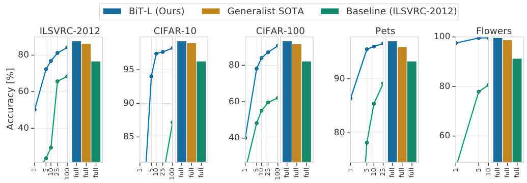
Fig. 1: Transfer performance of our pre-trained model, BiT-L, the previous stateof-the-art (SOTA), and a ResNet-50 baseline pre-trained on ILSVRC-2012 to downstream tasks. Here we consider only methods that are pre-trained independently of the final task (generalist representations), like BiT. The bars show the accuracy when fine-tuning on the full downstream dataset. The curve on the left-hand side of each plot shows that BiT-L performs well even when transferred using only few images (1 to 100) per class.
图 1: 我们预训练模型 BiT-L、先前最先进技术 (SOTA) 及基于 ILSVRC-2012 预训练的 ResNet-50 基线在下游任务中的迁移性能。此处仅考虑独立于最终任务预训练的方法 (通用表征) ,如 BiT。柱状图显示完整下游数据集微调后的准确率。每幅图左侧曲线表明,即使每类仅用少量图像 (1 至 100 张) 进行迁移,BiT-L 仍表现优异。
Importantly, BiT only needs to be pre-trained once and subsequent finetuning to downstream tasks is cheap. By contrast, other state-of-the-art methods require extensive training on support data conditioned on the task at hand [38,61,63]. Not only does BiT require a short fine-tuning protocol for each new task, but BiT also does not require extensive hyper parameter tuning on new tasks. Instead, we present a heuristic for setting the hyper parameters for transfer, which works well on our diverse evaluation suite.
重要的是,BiT只需预训练一次,后续针对下游任务的微调成本很低。相比之下,其他先进方法需要根据当前任务对支持数据进行大量训练[38,61,63]。BiT不仅对新任务只需简短微调流程,还无需在新任务上进行大量超参数调优。相反,我们提出了一种设定迁移超参数的启发式方法,在我们的多样化评估集中表现优异。
We highlight the most important components that make Big Transfer effective, and provide insight into the interplay between scale, architecture, and training hyper parameters. For practitioners, we will release the performant BiTM model trained on ImageNet-21k.
我们重点介绍了使Big Transfer高效的关键组件,并深入分析了规模、架构与训练超参数之间的相互作用。对于实践者,我们将发布基于ImageNet-21k训练的高性能BiTM模型。
2 Big Transfer
2 大迁移 (Big Transfer)
We review the components that we found necessary to build an effective network for transfer. Upstream components are those used during pre-training, and downstream are those used during fine-tuning to a new task.
我们回顾了构建有效迁移网络所需的组件。上游组件 (upstream components) 用于预训练阶段,下游组件 (downstream components) 用于新任务的微调阶段。
2.1 Upstream Pre-Training
2.1 上游预训练
The first component is scale. It is well-known in deep learning that larger networks perform better on their respective tasks [15,48]. Further, it is recognized that larger datasets require larger architectures to realize benefits, and vice versa [25,45]. We study the effectiveness of scale (during pre-training) in the context of transfer learning, including transfer to tasks with very few datapoints. We investigate the interplay between computational budget (training time), architecture size, and dataset size. For this, we train three BiT models on three large datasets: ILSVRC-2012 [46] which contains 1.3M images (BiT-S), ImageNet-21k [10] which contains 14M images (BiT-M), and JFT [51] which contains 300M images (BiT-L).
第一个要素是规模。深度学习领域众所周知,更大的网络在各自任务上表现更优[15,48]。此外,更大的数据集需要更大的架构才能发挥优势,反之亦然[25,45]。我们研究了预训练阶段规模对迁移学习效果的影响,包括数据点极少的任务迁移。我们重点探究了计算预算(训练时长)、架构规模与数据集大小之间的动态关系。为此,我们在三个大型数据集上训练了三个BiT模型:包含130万张图片的ILSVRC-2012[46](BiT-S)、包含1400万张图片的ImageNet-21k[10](BiT-M),以及包含3亿张图片的JFT[51](BiT-L)。
The second component is Group Normalization (GN) [60] and Weight Standar diz ation (WS) [34]. Batch Normalization (BN) [21] is used in most state-ofthe-art vision models to stabilize training. However, we find that BN is detrimental to Big Transfer for two reasons. First, when training large models with small per-device batches, BN performs poorly or incurs inter-device synchronization cost. Second, due to the requirement to update running statistics, BN is detrimental for transfer. GN, when combined with WS, has been shown to improve performance on small-batch training for ImageNet and COCO [34]. Here, we show that the combination of GN and WS is useful for training with large batch sizes, and has a significant impact on transfer learning.
第二个组件是分组归一化 (Group Normalization, GN) [60] 和权重标准化 (Weight Standardization, WS) [34]。大多数先进视觉模型使用批量归一化 (Batch Normalization, BN) [21] 来稳定训练。但我们发现BN对大规模迁移学习有两个不利影响:首先,在使用小批量设备训练大模型时,BN表现不佳或产生设备间同步成本;其次,由于需要更新运行统计量,BN不利于迁移学习。研究表明,GN与WS结合能提升ImageNet和COCO小批量训练性能[34]。本文进一步证明,GN+WS组合在大批量训练中同样有效,并对迁移学习产生显著影响。
2.2 Transfer to Downstream Tasks
2.2 迁移至下游任务
We propose a cheap fine-tuning protocol that applies to many diverse downstream tasks. Importantly, we avoid expensive hyper parameter search for every new task and dataset size; we try only one hyper parameter per task. We use a heuristic rule—which we call BiT-HyperRule—to select the most important hyper parameters for tuning as a simple function of the task’s intrinsic image resolution and number of datapoints. We found it important to set the following hyper parameters per-task: training schedule length, resolution, and whether to use MixUp regular iz ation [67]. We use BiT-HyperRule for over 20 tasks in this paper, with training sets ranging from 1 example per class to over 1M total examples. The exact settings for BiT-HyperRule are presented in Section 3.3.
我们提出了一种适用于多种下游任务的低成本微调方案。其核心在于避免为每个新任务和数据集规模进行昂贵超参数搜索,每个任务仅尝试一组超参数。我们采用名为BiT-HyperRule的启发式规则,根据任务固有图像分辨率和数据点数量来动态选择最关键的超参数。实践表明,必须针对每个任务设置以下超参数:训练周期长度、分辨率以及是否使用MixUp正则化[67]。本文在超过20个任务中应用了BiT-HyperRule,这些任务的训练集规模从每类1个样本到总数超100万样本不等。BiT-HyperRule的具体设置详见3.3节。
During fine-tuning, we use the following standard data pre-processing: we resize the image to a square, crop out a smaller random square, and randomly horizontally flip the image at training time. At test time, we only resize the image to a fixed size. In some tasks horizontal flipping or cropping destroys the label semantics, making the task impossible. An example is if the label requires predicting object orientation or coordinates in pixel space. In these cases we omit flipping or cropping when appropriate.
在微调过程中,我们采用以下标准数据预处理流程:将图像调整为正方形尺寸,随机裁剪出较小正方形区域,并在训练时随机进行水平翻转。测试阶段仅将图像缩放至固定尺寸。某些任务中水平翻转或裁剪会破坏标签语义(例如需预测物体朝向或像素空间坐标的任务),此时我们会视情况省略翻转或裁剪操作。
Recent work has shown that existing augmentation methods introduce inconsistency between training and test resolutions for CNNs [57]. Therefore, it is common to scale up the resolution by a small factor at test time. As an alternative, one can add a step at which the trained model is fine-tuned to the test resolution [57]. The latter is well-suited for transfer learning; we include the resolution change during our fine-tuning step.
规则:
- 输出中文翻译部分时仅保留翻译标题,无冗余内容,不重复不解释。
- 不输出无关内容。
- 保留原始段落格式及术语(如FLAC/JPEG)、公司缩写(如Microsoft/Amazon/OpenAI)。
- 人名不译。
- 保留文献引用标记如[20]。
- Figure/Table翻译为"图1: "/"表1: "并保留原格式。
- 全角括号转半角,左右括号添加半角空格。
- 专业术语首现标注英文(如"生成式AI (Generative AI)"),后续纯中文。
- AI术语对照:
- Transformer -> Transformer
- Token -> Token
- LLM -> 大语言模型
- Zero-shot -> 零样本
- Few-shot -> 少样本
- AI Agent -> AI智能体
- AGI -> 通用人工智能
- Python -> Python语言
策略:
- 特殊字符/公式原样保留
- HTML表格转Markdown格式
- 英译中需信息完整且符合中文习惯
最终:
作为替代方案,可在测试时增加一个步骤:对训练好的模型进行测试分辨率微调 [57] 。该方法特别适合迁移学习——我们在微调阶段同步完成分辨率调整。
We found that MixUp [67] is not useful for pre-training BiT, likely due to the abundance of data. However, it is sometimes useful for transfer. Interestingly, it is most useful for mid-sized datasets, and not for few-shot transfer, see Section 3.3 for where we apply MixUp.
我们发现 MixUp [67] 在预训练 BiT 时效果不佳,可能是由于数据量充足。但在迁移学习中偶尔有效。有趣的是,它对中等规模数据集最有效,而对少样本迁移无效,具体应用场景参见第 3.3 节。
Surprisingly, we do not use any of the following forms of regular iz ation during downstream tuning: weight decay to zero, weight decay to initial parameters [31], or dropout. Despite the fact that the network is very large—BiT has 928 million parameters—the performance is surprisingly good without these techniques and their respective hyper parameters, even when transferring to very small datasets. We find that setting an appropriate schedule length, i.e. training longer for larger datasets, provides sufficient regular iz ation.
令人惊讶的是,在下游调优过程中,我们没有使用以下任何一种正则化形式:权重衰减归零、权重衰减至初始参数 [31] 或 dropout。尽管网络规模非常大(BiT 拥有 9.28 亿参数),但在不使用这些技术及其相应超参数的情况下,性能依然出奇地好,甚至在迁移到极小数据集时也是如此。我们发现,设置适当的训练周期长度(即针对更大数据集延长训练时间)已能提供足够的正则化效果。
3 Experiments
3 实验
We train three upstream models using three datasets at different scales: BiT-S, BiT-M, and BiT-L. We evaluate these models on many downstream tasks and attain very strong performance on high and low data regimes.
我们使用三种不同规模的数据集训练了三个上游模型:BiT-S、BiT-M和BiT-L。这些模型在众多下游任务上进行了评估,并在高数据量和低数据量场景下均表现出色。
3.1 Data for Upstream Training
3.1 上游训练数据
BiT-S is trained on the ILSVRC-2012 variant of ImageNet, which contains 1.28 million images and 1000 classes. Each image has a single label. BiT-M is trained on the full ImageNet-21k dataset [10], a public dataset containing 14.2 million images and 21k classes organized by the WordNet hierarchy. Images may contain multiple labels. BiT-L is trained on the JFT-300M dataset [51,38,61]. This dataset is a newer version of that used in [18,8]. JFT-300M consists of around 300 million images with 1.26 labels per image on average. The labels are organized into a hierarchy of 18 291 classes. Annotation is performed using an automatic pipeline, and are therefore imperfect; approximately 20% of the labels are noisy. We remove all images present in downstream test sets from JFT-300M. See Supplementary Material section C for details. Note: the “-S/M/L” suffix refers to the pre-training datasets size and schedule, not architecture. We train BiT with several architecture sizes, the default (largest) being Res Net 152 x 4.
BiT-S在ImageNet的ILSVRC-2012版本上训练,包含128万张图像和1000个类别。每张图像有单一标签。BiT-M在完整的ImageNet-21k数据集[10]上训练,这是一个包含1420万张图像和2.1万个类别的公开数据集,按WordNet层次结构组织。图像可能包含多个标签。BiT-L在JFT-300M数据集[51,38,61]上训练。该数据集是[18,8]所用版本的新迭代,包含约3亿张图像,平均每张图像有1.26个标签,标签按18291个类别的层次结构组织。标注通过自动化流程完成,因此存在约20%的噪声标签。我们从JFT-300M中移除了所有下游测试集出现的图像。详见补充材料C部分。注:"-S/M/L"后缀指预训练数据集规模与训练计划,而非架构。我们使用多种架构规模训练BiT,默认(最大)为ResNet 152×4。
3.2 Downstream Tasks
3.2 下游任务
We evaluate BiT on long-standing benchmarks: ILSVRC-2012 [10], CIFAR10/100 [27], Oxford-IIIT Pet [41] and Oxford Flowers-102 [39]. These datasets differ in the total number of images, input resolution and nature of their categories, from general object categories in ImageNet and CIFAR to fine-grained ones in Pets and Flowers. We fine-tune BiT on the official training split and report results on the official test split if publicly available. Otherwise, we use the val split.
我们在长期基准测试上评估BiT:ILSVRC-2012 [10]、CIFAR10/100 [27]、Oxford-IIIT Pet [41]和Oxford Flowers-102 [39]。这些数据集在图像总数、输入分辨率和类别性质上存在差异,从ImageNet和CIFAR中的通用物体类别,到Pets和Flowers中的细粒度类别。我们在官方训练集上微调BiT,并在公开可用的官方测试集上报告结果。否则,我们使用验证集。
Table 1: Top-1 accuracy for BiT-L on many datasets using a single model and single hyper parameter setting per task (BiT-HyperRule). The entries show median $\pm$ standard deviation across 3 fine-tuning runs. Specialist models are those that condition pre-training on each task, while generalist models, including BiT, perform task-independent pre-training. ( $\star$ Concurrent work.)
| BiT-L | GeneralistSOTA | SpecialistSOTA | |
| ILSVRC-2012 | 87.54±0.02 | 86.4 [57] | 88.4 [61]* |
| CIFAR-10 | 99.37±0.06 | 99.0 [19] | |
| CIFAR-100 | 93.51±0.08 | 91.7 [55] | |
| Pets | 96.62±0.23 | 95.9 [19] | 97.1 [38] |
| Flowers | 99.63 ± 0.03 | 98.8 [55] | 97.7 [38] |
| VTAB (19 tasks) | 76.29 ± 1.70 | 70.5 [58] |
表 1: BiT-L在多个数据集上的Top-1准确率,使用单一模型和每个任务的单一超参数设置(BiT-HyperRule)。条目显示3次微调运行的中值$\pm$标准差。专家模型(Specialist)是指针对每个任务进行预训练的模型,而通用模型(Generalist)(包括BiT)执行与任务无关的预训练。( $\star$ 并发工作。)
| BiT-L | GeneralistSOTA | SpecialistSOTA | |
|---|---|---|---|
| ILSVRC-2012 | 87.54±0.02 | 86.4 [57] | 88.4 [61]* |
| CIFAR-10 | 99.37±0.06 | 99.0 [19] | |
| CIFAR-100 | 93.51±0.08 | 91.7 [55] | |
| Pets | 96.62±0.23 | 95.9 [19] | 97.1 [38] |
| Flowers | 99.63±0.03 | 98.8 [55] | 97.7 [38] |
| VTAB (19 tasks) | 76.29±1.70 | 70.5 [58] |
To further assess the generality of representations learned by BiT, we evaluate on the Visual Task Adaptation Benchmark (VTAB) [66]. VTAB consists of 19 diverse visual tasks, each of which has 1000 training samples (VTAB-1k variant). The tasks are organized into three groups: natural, specialized and structured. The VTAB-1k score is top-1 recognition performance averaged over these 19 tasks. The natural group of tasks contains classical datasets of natural images captured using standard cameras. The specialized group also contains images captured in the real world, but through specialist equipment, such as satellite or medical images. Finally, the structured tasks assess understanding of the the structure of a scene, and are mostly generated from synthetic environments. Example structured tasks include object counting and 3D depth estimation.
为了进一步评估BiT学习到的表征的通用性,我们在视觉任务适应基准(VTAB)[66]上进行了评估。VTAB包含19个不同的视觉任务,每个任务有1000个训练样本(VTAB-1k变体)。这些任务分为三组:自然、专业和结构化。VTAB-1k分数是这19个任务的平均top-1识别性能。自然类任务包含使用标准相机拍摄的自然图像的经典数据集。专业类任务也包含在现实世界中拍摄的图像,但通过专业设备获取,如卫星或医学图像。最后,结构化任务评估对场景结构的理解,大多来自合成环境。结构化任务的例子包括物体计数和3D深度估计。
3.3 Hyper parameter Details
3.3 超参数详情
Upstream Pre-Training All of our BiT models use a vanilla ResNet-v2 architecture [16], except that we replace all Batch Normalization [21] layers with Group Normalization [60] and use Weight Standardization [43] in all convolutional layers. See Section 4.3 for analysis. We train ResNet-152 architectures in all datasets, with every hidden layer widened by a factor of four (Res Net 152 x 4). We study different model sizes and the coupling with dataset size in Section 4.1.
上游预训练
我们所有的BiT模型都使用标准的ResNet-v2架构[16],只是将所有批归一化(Batch Normalization)[21]层替换为组归一化(Group Normalization)[60],并在所有卷积层中使用权重标准化(Weight Standardization)[43]。具体分析见第4.3节。我们在所有数据集中训练ResNet-152架构,每个隐藏层都加宽了四倍(ResNet152x4)。第4.1节将研究不同模型规模与数据集规模的耦合关系。
We train all of our models upstream using SGD with momentum. We use an initial learning rate of 0.03, and momentum 0.9. During image preprocessing stage we use image cropping technique from [53] and random horizontal mirroring followed by $224\times224$ image resize. We train both BiT-S and BiT-M for 90 epochs and decay the learning rate by a factor of 10 at 30, 60 and 80 epochs. For BiT-L, we train for 40 epochs and decay the learning rate after 10, 23, 30 and 37 epochs. We use a global batch size of 4096 and train on a Cloud TPUv3- 512 [24], resulting in 8 images per chip. We use linear learning rate warm-up for 5000 optimization steps and multiply the learning rate by batch size following [11]. During pre-training we use a weight decay of 0.0001, but as discussed in Section 2, we do not use any weight decay during transfer.
我们在上游训练所有模型时采用带动量的随机梯度下降法(SGD),初始学习率为0.03,动量参数为0.9。图像预处理阶段采用[53]提出的裁剪技术,并随机进行水平镜像翻转后调整至$224\times224$分辨率。BiT-S和BiT-M模型均训练90个周期,在第30、60和80周期时将学习率衰减为原值的1/10;BiT-L模型训练40个周期,在第10、23、30和37周期时进行学习率衰减。全局批量大小设为4096,使用Cloud TPUv3-512[24]进行训练,每个芯片处理8张图像。按照[11]的方法,我们采用5000次优化步骤的线性学习率预热,并将学习率与批量大小相乘。预训练阶段权重衰减系数设为0.0001,但如第2节所述,迁移学习时不使用任何权重衰减。
Table 2: Improvement in accuracy when pre-training on the public ImageNet-21k dataset over the “standard” ILSVRC-2012. Both models are Res Net 152 x 4.
| ILSVRC- 2012 | CIFAR- 10 | CIFAR- 100 | Pets | Flowers | VTAB-1k (19 tasks) | |
| BiT-S (ILSVRC-2012) | 81.30 | 97.51 | 86.21 | 93.97 | 89.89 | 66.87 |
| BiT-M (ImageNet-21k) | 85.39 | 98.91 | 92.17 | 94.46 | 99.30 | 70.64 |
| Improvement | +4.09 | +1.40 | +5.96 | +0.49 | +9.41 | +3.77 |
表 2: 在公开数据集ImageNet-21k上预训练相比"标准"ILSVRC-2012带来的准确率提升。两个模型均为ResNet-152x4。
| ILSVRC-2012 | CIFAR-10 | CIFAR-100 | Pets | Flowers | VTAB-1k (19 tasks) | |
|---|---|---|---|---|---|---|
| BiT-S (ILSVRC-2012) | 81.30 | 97.51 | 86.21 | 93.97 | 89.89 | 66.87 |
| BiT-M (ImageNet-21k) | 85.39 | 98.91 | 92.17 | 94.46 | 99.30 | 70.64 |
| Improvement | +4.09 | +1.40 | +5.96 | +0.49 | +9.41 | +3.77 |
Downstream Fine-Tuning To attain a low per-task adaptation cost, we do not perform any hyper parameter sweeps downstream. Instead, we present BiTHyperRule, a heuristic to determine all hyper parameters for fine-tuning. Most hyper parameters are fixed across all datasets, but schedule, resolution, and usage of MixUp depend on the tasks image resolution and training set size.
下游微调
为降低每项任务的适应成本,我们未在下游进行任何超参数扫描。相反,我们提出了BiTHyperRule——一种用于确定微调所有超参数的启发式方法。大多数超参数在所有数据集中固定不变,但调度策略、分辨率以及MixUp的使用取决于任务的图像分辨率和训练集规模。
For all tasks, we use SGD with an initial learning rate of 0.003, momentum 0.9, and batch size 512. We resize input images with area smaller than $96\times96$ pixels to $160\times160$ pixels, and then take a random crop of $128\times128$ pixels. We resize larger images to $448\times448$ and take a $384\times384$ -sized crop.1 We apply random crops and horizontal flips for all tasks, except those for which cropping or flipping destroys the label semantics, see Supplementary section F for details.
对于所有任务,我们使用初始学习率为0.003、动量为0.9、批量大小为512的SGD优化器。将面积小于$96\times96$像素的输入图像缩放至$160\times160$像素后,随机裁剪出$128\times128$像素区域;较大图像则缩放至$448\times448$像素后裁剪$384\times384$像素区域。除会破坏标签语义的任务外(详见补充材料F部分),所有任务均应用随机裁剪和水平翻转。
For schedule length, we define three scale regimes based on the number of examples: we call small tasks those with fewer than $20\mathrm{k\Omega}$ labeled examples, medium those with fewer than $500\mathrm{k\Omega}$ , and any larger dataset is a large task. We fine-tune BiT for 500 steps on small tasks, for 10k steps on medium tasks, and for 20k steps on large tasks. During fine-tuning, we decay the learning rate by a factor of 10 at $30%$ , $60%$ and 90% of the training steps. Finally, we use MixUp [67], with $\alpha=0.1$ , for medium and large tasks. See Supplementary section A for details.
对于训练时长,我们根据样本数量定义了三种规模级别:少于$20\mathrm{k\Omega}$标注样本的任务称为小型任务,少于$500\mathrm{k\Omega}$的为中型任务,更大的数据集则归类为大型任务。我们在小型任务上对BiT进行500步微调,中型任务10k步,大型任务20k步。微调过程中,学习率在训练步数达到30%、60%和90%时分别衰减为原来的1/10。对于中型和大型任务,我们使用MixUp [67](参数$\alpha=0.1$)。详见补充材料A节。
3.4 Standard Computer Vision Benchmarks
3.4 标准计算机视觉基准测试
We evaluate BiT-L on standard benchmarks and compare its performance to the current state-of-the-art results (Table 1). We separate models that perform taskindependent pre-training (“general” representations), from those that perform task-dependent auxiliary training (“specialist” representations). The specialist methods condition on a particular task, for example ILSVRC-2012, then train using a large support dataset, such as JFT-300M [38] or Instagram-1B [63]. See discussion in Section 5. Specialist representations are highly effective, but require a large training cost per task. By contrast, generalized representations require large-scale training only once, followed by a cheap adaptation phase.
我们在标准基准上评估BiT-L,并将其性能与当前最先进的结果进行比较(表1)。我们将执行任务无关预训练的模型("通用"表示)与执行任务相关辅助训练的模型("专家"表示)区分开来。专家方法针对特定任务(例如ILSVRC-2012)进行条件化,然后使用大型支持数据集(如JFT-300M[38]或Instagram-1B[63])进行训练。详见第5节的讨论。专家表示非常有效,但每个任务都需要高昂的训练成本。相比之下,通用表示只需进行一次大规模训练,随后是一个低成本的适应阶段。
BiT-L outperforms previously reported generalist SOTA models as well as, in many cases, the SOTA specialist models. Inspired by strong results of BiT-L trained on JFT-300M, we also train models on the public ImageNet-21k dataset.
BiT-L 的表现优于先前报道的通用 SOTA 模型,并且在许多情况下也优于 SOTA 专业模型。受 BiT-L 在 JFT-300M 数据集上训练的优异结果启发,我们还在公开的 ImageNet-21k 数据集上训练了模型。
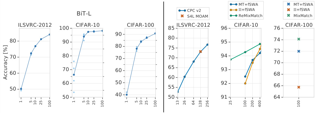
Fig. 2: Experiments in the low data regime. Left: Transfer performance of BiT-L. Each point represents the result after training on a balanced random subsample of the dataset (5 subsamples per dataset). The median across runs is highlighted by the curves. The variance across data samples is usually low, with the exception of 1-shot CIFAR-10, which contains only 10 images. Right: We summarize the state-of-the-art in semi-supervised learning as reference points. Note that a direct comparison is not meaningful; unlike BiT, semi-supervised methods have access to extra unlabelled data from the training distribution, but they do not make use of out-of-distribution labeled data.
图 2: 低数据量下的实验结果。左图: BiT-L的迁移性能。每个点代表在数据集平衡随机子样本(每个数据集5个子样本)上训练后的结果。曲线突出显示了多次运行的中位数结果。除仅含10张图像的1-shot CIFAR-10外,不同数据样本间的方差通常较低。右图: 我们总结了半监督学习的最新成果作为参考点。需注意直接对比并无意义;与BiT不同,半监督方法可以获取训练分布中的额外未标注数据,但不会利用分布外的标注数据。
This dataset is more than 10 times bigger than ILSVRC-2012, but it is mostly overlooked by the research community. In Table 2 we demonstrate that BiT-M trained on ImageNet-21k leads to substantially improved visual representations compared to the same model trained on ILSVRC-2012 (BiT-S), as measured by all our benchmarks. In Section 4.2, we discuss pitfalls that may have hindered wide adoption of ImageNet-21k as a dataset model for pre-training and highlight crucial components of BiT that enabled success on this large dataset.
该数据集规模是ILSVRC-2012的10倍以上,但大多被研究界忽视。如表2所示,通过我们的所有基准测试衡量,在ImageNet-21k上训练的BiT-M比在ILSVRC-2012上训练的相同模型(BiT-S)显著提升了视觉表征能力。在4.2节中,我们讨论了可能阻碍ImageNet-21k作为预训练数据集被广泛采用的潜在问题,并重点介绍了BiT在这个大型数据集上取得成功的关键组件。
For completeness, we also report top-5 accuracy on ILSVRC-2012 with median $\pm$ standard deviation format across 3 runs: 98.46% 0.02% for BiT-L, $97.69%\pm0.02%$ for BiT-M and 95.65% 0.03% for BiT-S.
为了完整性,我们还在ILSVRC-2012上报告了top-5准确率(以3次运行的中位数$\pm$标准差格式): BiT-L为$98.46%\pm0.02%$,BiT-M为$97.69%\pm0.02%$,BiT-S为$95.65%\pm0.03%$。
3.5 Tasks with Few Datapoints
3.5 少数据点任务
We study the number of downstream labeled samples required to transfer BiT-L successfully. We transfer BiT-L using subsets of ILSVRC-2012, CIFAR-10, and CIFAR-100, down to 1 example per class. We also evaluate on a broader suite of 19 VTAB-1k tasks, each of which has 1000 training examples.
我们研究了成功迁移BiT-L所需的下游标注样本数量。我们在ILSVRC-2012、CIFAR-10和CIFAR-100的子集上进行迁移实验,逐步减少每类样本至1个。同时,我们在包含19个任务的VTAB-1k基准上进行评估,每个任务提供1000个训练样本。
Figure 2 (left half) shows BiT-L using few-shots on ILSVRC-2012, CIFAR10, and CIFAR-100. We run multiple random subsamples, and plot every trial. Surprisingly, even with very few samples per class, BiT-L demonstrates strong performance and quickly approaches performance of the full-data regime. In particular, with just 5 labeled samples per class it achieves top-1 accuracy of $72.0%$ on ILSVRC-2012 and with 100 samples the top-1 accuracy goes to $84.1%$ . On CIFAR-100, we achieve $82.6%$ with just 10 samples per class.
图 2 (左半部分)展示了BiT-L在ILSVRC-2012、CIFAR10和CIFAR-100数据集上使用少样本(few-shot)学习的效果。我们进行了多次随机子采样,并绘制了每次试验结果。令人惊讶的是,即使每类只有极少样本,BiT-L仍展现出强劲性能,并快速接近全数据训练的效果。具体而言,在ILSVRC-2012上每类仅需5个标注样本就能达到72.0%的top-1准确率,100个样本时准确率升至84.1%。在CIFAR-100上,每类仅需10个样本即可达到82.6%的准确率。
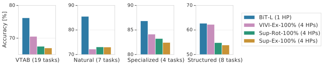
Fig. 3: Results on VTAB (19 tasks) with 1000 examples/task, and the current SOTA. It compares methods that sweep few hyper parameters per task: either four hyper parameters in previous work $\mathrm{^{\circ}4H P s^{,}\rangle}$ ) or the single BiT-HyperRule.
图 3: 在VTAB(19个任务)上每任务使用1000个样本的测试结果及当前SOTA。比较了每个任务只需调整少量超参数的方法:要么是先前工作中调整四个超参数的方案( $\mathrm{^{\circ}4H P s^{,}\rangle}$ ),要么是单一的BiT-HyperRule。
Semi-supervised learning also tackles learning with few labels. However, such approaches are not directly comparable to BiT. BiT uses extra labelled out-ofdomain data, whereas semi-supervised learning uses extra unlabelled in-domain data. Nevertheless, it is interesting to observe the relative benefits of transfer from out-of-domain labelled data versus in-domain semi-supervised data. In Figure 2 we show state-of-the-art results from the semi-supervised learning.
半监督学习同样致力于解决少标签学习问题。然而这类方法与BiT并不直接可比:BiT使用额外的跨领域标注数据,而半监督学习使用额外的同领域未标注数据。不过观察跨领域标注数据迁移与同领域半监督数据之间的相对优势仍颇具意义。图2展示了半监督学习领域的最先进成果。
Figure 3 shows the performance of BiT-L on the 19 VTAB-1k tasks. BiT-L with BiT-HyperRule substantially outperforms the previously reported state-ofthe-art. When looking into performance of VTAB-1k task subsets, BiT is the best on natural, specialized and structured tasks. The recently-proposed VIVIEx-100% [58] model that employs video data during upstream pre-training shows very similar performance on the structured tasks.
图 3: 展示了 BiT-L 在 19 个 VTAB-1k 任务上的性能表现。采用 BiT-HyperRule 的 BiT-L 显著超越了先前报道的最先进水平。在分析 VTAB-1k 任务子集的性能时,BiT 在自然、专业和结构化任务中均表现最佳。最近提出的 VIVIEx-100% [58] 模型在上游预训练阶段使用了视频数据,其在结构化任务上的表现与 BiT 非常接近。
We investigate heavy per-task hyper parameter tuning in Supplementary Material section A and conclude that this further improves performance.
我们在补充材料A部分研究了针对每个任务的重度超参数调优,并得出结论认为这能进一步提升性能。
3.6 ObjectNet: Recognition on a “Real-World” Test Set
3.6 ObjectNet: 在“真实世界”测试集上的识别
We evaluate BiT on the new test-only ObjectNet dataset [2]. Importantly, this dataset closely resembles real-life scenarios, where object categories may appear in non-canonical context, viewpoint, rotation, etc. There are 313 object classes in total, with 113 overlapping with ILSVRC2012. We follow the literature [2,6] and evaluate our models on those 113 classes.
我们在新的仅用于测试的ObjectNet数据集[2]上评估BiT。值得注意的是,该数据集高度贴近现实场景,物体类别可能出现在非标准背景、视角或旋转等条件下。数据集共包含313个物体类别,其中113个与ILSVRC2012重叠。我们遵循文献[2,6]的方法,在这113个类别上评估模型。
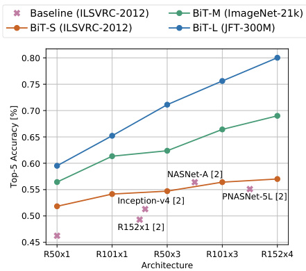
Fig. 4: Accuracy of BiT models along with baselines on ObjectNet. R is short for ResNet in x-axis.
图 4: BiT模型及基线在ObjectNet上的准确率。横轴R代表ResNet。
Figure 4 shows that larger architectures and pre-training on more data results in higher accuracies. Crucially, our results highlight that scaling both is essential for achieving unprecedented top-5 accuracy of $80.0%$ , an almost 25% absolute improvement over the previous state-of-the-art. We provide numeric results and additional results when classifying individual object bounding boxes [6] in the Supplementary Material section B.
图 4 表明,更大的架构和更多数据的预训练会带来更高的准确率。关键的是,我们的结果强调,同时扩展这两者对实现前所未有的 80.0% 的 top-5 准确率至关重要,这比之前的最先进水平提高了近 25% 的绝对值。我们在补充材料 B 部分提供了数值结果以及对单个物体边界框 [6] 进行分类时的额外结果。
3.7 Object Detection
3.7 目标检测
Finally, we evaluate BiT on object detection. We use the COCO-2017 dataset [34] and train a top-performing object detector, RetinaNet [33], using pre-trained BiT models as backbones. Due to memory constraints, we use the ResNet-101x3 architecture for all of our BiT models. We fine-tune the detection models on the COCO-2017 train split and report results on the validation split using the standard metric [34] in Table 3. Here, we do not use BiT-HyperRule, but stick to the standard RetinaNet training protocol, see the Supplementary Material
最后,我们在目标检测任务上评估BiT。使用COCO-2017数据集[34]并训练高性能目标检测器RetinaNet[33],将预训练的BiT模型作为骨干网络。由于内存限制,所有BiT模型均采用ResNet-101x3架构。我们在COCO-2017训练集上微调检测模型,并按照标准指标[34]在验证集上报告结果(见表3)。此处未使用BiT-HyperRule,而是遵循标准RetinaNet训练协议,详见补充材料。
section E for details. Table 3 demonstrates that BiT models outperform standard ImageNet pretrained models. We can see clear benefits of pre-training on large data beyond ILSVRC-2012: pretraining on ImageNet-21k results in a 1.5 point improvement in Average Precision (AP), while pretraining on JFT-300M further improves performance by 0.6 points.
详情见E节。表3表明BiT模型优于标准的ImageNet预训练模型。我们可以看到在ILSVRC-2012之外的大规模数据上进行预训练的明显优势:在ImageNet-21k上预训练使平均精度(AP)提高了1.5个百分点,而在JFT-300M上预训练则进一步将性能提升了0.6个百分点。
| Model | Upstream data | AP |
| RetinaNet 33 | ILSVRC-2012 | 40.8 |
| RetinaNet BiT-S) RetinaNet BiT-M) RetinaNet (BiT-L) | ILSVRC-2012 ImageNet-21k | 41.7 43.2 |
| 模型 | 上游数据 | AP |
|---|---|---|
| RetinaNet 33 | ILSVRC-2012 | 40.8 |
| RetinaNet BiT-S) RetinaNet BiT-M) RetinaNet (BiT-L) | ILSVRC-2012 ImageNet-21k | 41.7 43.2 |
Table 3: Object detection performance on COCO-2017 [34] validation data of RetinaNet models with pre-trained BiT backbones and the literature baseline.
表 3: 采用预训练 BiT 主干网络的 RetinaNet 模型及文献基线在 COCO-2017 [34] 验证集上的目标检测性能
4 Analysis
4 分析
We analyse various components of BiT: we demonstrate the importance of model capacity, discuss practical optimization caveats and choice of normalization layer.
我们分析了BiT的各个组成部分:展示了模型容量的重要性,讨论了实际优化中的注意事项以及归一化层的选择。
4.1 Scaling Models and Datasets
4.1 模型与数据集的扩展
The general consensus is that larger neural networks result in better performance. We investigate the interplay between model capacity and upstream dataset size on downstream performance. We evaluate the BiT models of different sizes (ResNet-50x1, ResNet-50x3, ResNet-101x1, ResNet-101x3, and ResNet-152x4) trained on ILSVRC-2012, ImageNet-21k, and JFT-300M on various downstream benchmarks. These results are summarized in Figure 5.
普遍认为更大的神经网络会带来更好的性能。我们研究了模型容量与上游数据集规模对下游性能的交互影响。评估了在不同上游数据集(ILSVRC-2012、ImageNet-21k和JFT-300M)上训练的多种规模BiT模型(ResNet-50x1、ResNet-50x3、ResNet-101x1、ResNet-101x3和ResNet-152x4)在多个下游基准测试中的表现。这些结果总结在图5中。
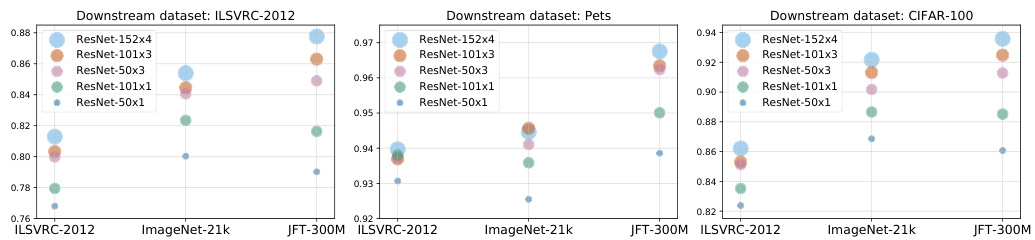
Fig. 5: Effect of upstream data (shown on the x-axis) and model size on downstream performance. Note that exclusively using more data or larger models may hurt performance; instead, both need to be increased in tandem.
图 5: 上游数据(x轴所示)和模型规模对下游性能的影响。请注意,仅增加数据量或扩大模型规模可能损害性能;相反,两者需要同步提升。
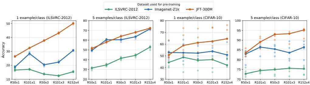
Fig. 6: Performance of BiT models in the low-data regime. The x-axis corresponds to the architecture, where R is short for ResNet. We pre-train on the three upstream datasets and evaluate on two downstream datasets: ILSVRC-2012 (left) and CIFAR-10 (right) with 1 or 5 examples per class. For each scenario, we train 5 models on random data subsets, represented by the lighter dots. The line connects the medians of these five runs.
图 6: BiT模型在低数据量场景下的性能表现。x轴表示网络架构,其中R是ResNet的缩写。我们在三个上游数据集上进行预训练,并在两个下游数据集上评估:ILSVRC-2012(左)和CIFAR-10(右),每类使用1或5个样本。每种情况下,我们在随机数据子集上训练5个模型(用浅色点表示),折线连接这五次运行的中值结果。
When pre-training on ILSVRC-2012, the benefit from larger models diminishes. However, the benefits of larger models are more pronounced on the larger two datasets. A similar effect is observed when training on Instagram hashtags [36] and in language modelling [25].
在ILSVRC-2012上进行预训练时,更大模型的收益会递减。但在更大的两个数据集上,大模型的优势更为显著。在Instagram标签训练[36]和语言建模[25]中也观察到了类似效应。
Not only is there limited benefit of training a large model size on a small dataset, but there is also limited (or even negative) benefit from training a small model on a larger dataset. Perhaps surprisingly, the ResNet-50x1 model trained on the JFT-300M dataset can even performs worse than the same architecture trained on the smaller ImageNet-21k. Thus, if one uses only a ResNet50x1, one may conclude that scaling up the dataset does not bring any additional benefits. However, with larger architectures, models pre-trained on JFT-300M significantly outperform those pre-trained on ILSVRC-2012 or ImageNet-21k.
在小数据集上训练大模型不仅收益有限,在大数据集上训练小模型同样收效甚微(甚至可能产生负面效果)。令人意外的是,在JFT-300M数据集上训练的ResNet-50x1模型表现甚至可能差于在较小规模ImageNet-21k上训练的相同架构。因此,若仅使用ResNet50x1架构,可能会得出扩大数据集无法带来额外收益的结论。但采用更大架构时,基于JFT-300M预训练的模型表现显著优于基于ILSVRC-2012或ImageNet-21k预训练的模型。
Figure 2 shows that BiT-L attains strong results even on tiny downstream datasets. Figure 6 ablates few-shot performance across different pre-training datasets and architectures. In the extreme case of one example per class, larger architectures outperform smaller ones when pre-trained on large upstream data. Interestingly, on ILSVRC-2012 with few shots, BiT-L trained on JFT-300M outperforms the models trained on the entire ILSVRC-2012 dataset itself. Note that for comparability, the classifier head is re-trained from scratch during fine-tuning, even when transferring ILSVRC-2012 full to ILSVRC-2012 few shot.
图 2 显示,BiT-L 即使在下游数据集极小的情况下也能取得强劲结果。图 6 对不同预训练数据集和架构的少样本性能进行了消融实验。在每类仅有一个样本的极端情况下,当上游数据规模较大时,较大架构的表现优于较小架构。值得注意的是,在 ILSVRC-2012 的少样本场景中,基于 JFT-300M 训练的 BiT-L 表现优于直接在整个 ILSVRC-2012 数据集上训练的模型。需要说明的是,为确保可比性,在微调阶段分类器头均从头开始重新训练,即使是从 ILSVRC-2012 完整数据集迁移到 ILSVRC-2012 少样本场景时也是如此。
4.2 Optimization on Large Datasets
4.2 大规模数据集优化
For standard computer vision datasets such as ILSVRC-2012, there are wellknown training procedures that are robust and lead to good performance. Progress in high-performance computing has made it feasible to learn from much larger datasets, such as ImageNet-21k, which has 14.2M images compared to ILSVRC2012’s 1.28M. However, there are no established procedures for training from such large datasets. In this section we provide some guidelines.
对于ILSVRC-2012等标准计算机视觉数据集,存在稳健且能带来良好性能的成熟训练流程。高性能计算的进步使得从更大规模数据集(如包含1420万张图像的ImageNet-21k,而ILSVRC-2012仅有128万张)学习成为可能。然而针对此类超大规模数据集的训练尚未形成标准流程,本节将提供若干指导原则。
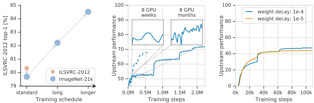
Fig. 7: Left: Applying the “standard” computational budget of ILSVRC-2012 to the larger ImageNet-21k seems detrimental. Only when we train longer (3x and 10x) do we see the benefits of training on the larger dataset. Middle: The learning progress of a ResNet-101x3 on JFT-300M seems to be flat even after 8 GPU-weeks, but after 8 GPU-months progress is clear. If one decays the learning rate too early (dashed curve), final performance is significantly worse. Right: Faster initial convergence with lower weight decay may trick the practitioner into selecting a sub-optimal value. Higher weight decay converges more slowly, but results in a better final model.
图 7: 左图: 将ILSVRC-2012的"标准"计算预算应用于更大的ImageNet-21k数据集似乎有害。只有当我们训练更长时间(3倍和10倍)时,才能看到在更大数据集上训练的好处。中图: ResNet-101x3在JFT-300M上的学习进度即使在8个GPU周后似乎也很平缓,但在8个GPU月后进展明显。如果过早降低学习率(虚线曲线),最终性能会明显变差。右图: 较低权重衰减带来的初始收敛速度更快,可能会误导实践者选择次优值。较高的权重衰减收敛速度较慢,但能产生更好的最终模型。
Sufficient computational budget is crucial for training performant models on large datasets. The standard ILSVRC-2012 training schedule processes roughly 100 million images (1.28M images $\times$ 90 epochs). However, if the same computational budget is applied to ImageNet-21k, the resulting model performs worse on ILSVRC-2012, see Figure 7, left. Nevertheless, as shown in the same figure, by increasing the computational budget, we not only recover ILSVRC-2012 performance, but significantly outperforms it. On JFT-300M the validation error may not improve over a long time —Figure 7 middle plot, “8 GPU weeks” zoom-in— although the model is still improving as evidenced by the longer time window.
充足的计算预算对于在大型数据集上训练高性能模型至关重要。标准ILSVRC-2012训练方案大约处理1亿张图像(1.28M图像×90轮次)。但若将相同计算预算应用于ImageNet-21k,所得模型在ILSVRC-2012上表现更差(见图7左)。然而如该图所示,通过增加计算预算,我们不仅能恢复ILSVRC-2012性能,还能显著超越它。在JFT-300M上,验证误差可能长期未见改善(图7中图"8GPU周"放大区域),但更长时间窗口显示模型仍在持续优化。
Another important aspect of pre-training with large datasets is the weight decay. Lower weight decay can result in an apparent acceleration of convergence, Figure 7 rightmost plot. However, this setting eventually results in an under-performing final model. This counter-intuitive behavior stems from the interaction of weight decay and normalization layers [29,32]. Low weight decay results in growing weight norms, which in turn results in a diminishing effective learning rate. Initially this effect creates an impression of faster convergence, but it eventually prevents further progress. A sufficiently large weight decay is required to avoid this effect, and throughout we use $10^{-4}$ .
在大数据集上进行预训练的另一个重要方面是权重衰减 (weight decay)。较低的权重衰减会导致收敛速度明显加快,如图 7 最右侧图表所示。然而,这种设置最终会导致模型性能不佳。这种反直觉行为源于权重衰减与归一化层 [29,32] 的相互作用。低权重衰减会导致权重范数增长,进而导致有效学习率下降。最初这种效应会让人产生收敛速度加快的错觉,但最终会阻碍进一步进展。为避免这种效应,需要使用足够大的权重衰减,本文全程采用 $10^{-4}$。
Finally, we note that in all of our experiments we use stochastic gradient descent with momentum without any modifications. In our preliminary experiments we did not observe benefits from more involved adaptive gradient methods.
最后,我们注意到在所有实验中均使用了未加修改的带动量的随机梯度下降法。在初步实验中,我们并未观察到更复杂的自适应梯度方法带来优势。
Table 4: Top-1 accuracy of ResNet-50 trained from scratch on ILSVRC-2012 with a batch-size of 4096.
| Plain Conv | Weight Std. | |
| Batch Norm. | 75.6 | 75.8 |
| Group Norm. | 70.2 | 76.0 |
表 4: 在ILSVRC-2012数据集上以4096批量大小从头训练的ResNet-50的Top-1准确率。
| Plain Conv | Weight Std. | |
|---|---|---|
| Batch Norm. | 75.6 | 75.8 |
| Group Norm. | 70.2 | 76.0 |
Table 5: Transfer performance of the corresponding models from Table 4 fine-tuned to the 19 VTAB-1k tasks.
| Plain Conv | Weight Std. | |
| Batch Norm. | 67.72 | 66.78 |
| Group Norm. | 68.77 | 70.39 |
表 5: 表 4 中对应模型在 19 个 VTAB-1k 任务上微调后的迁移性能
| Plain Conv | Weight Std. | |
|---|---|---|
| Batch Norm. | 67.72 | 66.78 |
| Group Norm. | 68.77 | 70.39 |
4.3 Large Batches, Group Normalization, Weight Standardization
4.3 大批量训练、组归一化与权重标准化
Currently, training on large datasets is only feasible using many hardware accelerators. Data parallelism is the most popular distribution strategy, and this naturally entails large batch sizes. Many known algorithms for training with large batch sizes use Batch Normalization (BN) [21] as a component [12] or even highlight it as the key instrument required for large batch training [9].
目前,只有使用大量硬件加速器才能在大规模数据集上进行训练。数据并行是最流行的分布式策略,这自然需要大批量训练。许多已知的大批量训练算法都将批归一化 (BN) [21] 作为核心组件 [12],甚至强调它是大批量训练所需的关键工具 [9]。
Our larger models have a high memory requirement for any single accelerator chip, which necessitates small per-device batch sizes. However, BN performs worse when the number of images on each accelerator is too low [20]. An alternative strategy is to accumulate BN statistics across all of the accelerators. However, this has two major drawbacks. First, computing BN statistics across large batches has been shown to harm generalization [9]. Second, using global BN requires many aggregations across accelerators which incurs significant latency.
我们的大模型对任何单个加速器芯片都有较高的内存需求,这导致每个设备的批量大小较小。然而,当每个加速器上的图像数量过少时,批量归一化 (BN) 的表现会变差 [20]。另一种策略是在所有加速器上累积 BN 统计量,但这存在两个主要缺点。首先,研究表明在大批量上计算 BN 统计量会损害泛化性能 [9]。其次,使用全局 BN 需要在加速器之间进行大量聚合,这会带来显著的延迟。
We investigated Group Normalization (GN) [60] and Weight Standardization (WS) [43] as alternatives to BN. We tested large batch training using 128 accelerator chips and a batch size of 4096. We found that GN alone does not scale to large batches; we observe a performance drop of $5.4%$ on ILSVRC-2012 top-1 accuracy compared to using BN in a ResNet-50x1. The addition of WS enables GN to scale to such large batches, even outperforming BN, see Table 4.
我们研究了组归一化 (Group Normalization, GN) [60] 和权重标准化 (Weight Standardization, WS) [43] 作为批量归一化 (BN) 的替代方案。测试采用128块加速芯片和4096批量进行大规模批次训练。发现单独使用GN无法扩展到大批量场景:在ResNet-50x1模型中,与使用BN相比,ILSVRC-2012 top-1准确率下降了$5.4%$。加入WS后GN可适配该批量规模,其表现甚至超越BN,详见表4。
We are not only interested in upstream performance, but also how models trained with GN and WS transfer. We thus transferred models with different combinations of BN, GN, and WS pre-trained on ILSVRC-2012 to the 19 tasks defined by VTAB. The results in Table 5 indicate that the GN/WS combination transfers better than BN, so we use GN/WS in all BiT models.
我们不仅关注上游性能,还研究了使用GN和WS训练的模型迁移效果。为此,我们将ILSVRC-2012上预训练的不同BN、GN、WS组合模型迁移到VTAB定义的19个任务中。表5结果显示,GN/WS组合的迁移效果优于BN,因此所有BiT模型均采用GN/WS方案。
5 Related Work
5 相关工作
Large-scale Weakly Supervised Learning of Representations A number of prior works use large supervised datasets for pre-training visual representations [23,51,30,36]. In [23,30] the authors use a dataset containing 100M Flickr images [56]. This dataset appears to transfer less well than JFT-300M.While studying the effect of dataset size, [51] show good transfer performance when training on JFT-300M, despite reporting a large degree of noise (20% precision errors) in the labels. An even larger, noisily labelled dataset of 3.5B Instagram images is used in [36]. This increase in dataset size and an improved model architecture [62] lead to better results when transferring to ILSVRC-2012. We show that we can attain even better performance with ResNet using JFT-300M with appropriate adjustments presented in Section 2. The aforementioned papers focus on transfer to ImageNet classification, and COCO or VOC detection and segmentation. We show that transfer is also highly effective in the low data regime, and works well on the broader set of 19 tasks in VTAB [66].
大规模弱监督学习的表征方法
多项先前研究利用大型监督数据集进行视觉表征的预训练 [23,51,30,36]。在 [23,30] 中,作者使用了包含1亿张Flickr图像的数据集 [56]。该数据集的迁移效果似乎不如JFT-300M。在研究数据集规模的影响时,[51] 表明尽管标签存在大量噪声(20%的精度误差),但在JFT-300M上训练时仍能获得良好的迁移性能。[36] 则使用了更大规模的噪声标注数据集,包含35亿张Instagram图像。数据集规模的增加以及改进的模型架构 [62] 使得迁移到ILSVRC-2012时取得了更好的结果。我们证明,通过第2节介绍的适当调整,使用ResNet和JFT-300M可以获得更优的性能。上述论文主要关注迁移到ImageNet分类以及COCO或VOC检测与分割任务。我们证明了在低数据量场景下迁移同样非常有效,并且在VTAB [66] 的19个任务上表现良好。
Specialized Representations Rather than pre-train generic representations, recent works have shown strong performance by training task-specific representations [63,38,61]. These papers condition on a particular task when training on a large support dataset. [63,61] train student networks on a large unlabelled support dataset using the predictions of a teacher network trained on the target task. [38] compute importance weights on the a labelled support dataset by conditioning on the target dataset. They then train the representations on the re-weighted source data. Even though these approaches may lead to superior results, they require knowing the downstream dataset in advance and substantial computational resources for each downstream dataset.
专业化表征
近期研究表明,通过训练任务特定表征(而非预训练通用表征)可获得强劲性能 [63,38,61]。这些论文在大型支持数据集训练时,会针对特定任务进行条件化处理。[63,61] 利用目标任务训练的教师网络预测结果,在未标注的大型支持数据集上训练学生网络。[38] 则通过以目标数据集为条件,在标注的支持数据集上计算重要性权重,随后基于重加权源数据训练表征。尽管这些方法可能带来更优结果,但需要提前了解下游数据集,并为每个下游数据集投入大量计算资源。
Unsupervised and Semi-Supervised Representation learning Self-supervised methods have shown the ability to leverage unsupervised datasets to transfer to labelled tasks. For example, [13] show that unsupervised representations trained on 1B unlabelled Instagram images transfer comparably or better than supervised ILSVRC-2012 features. Semi-supervised learning exploits unsupervised data drawn from the same domain as the labelled data. [5,50] used semi-supervised learning to attain strong performance on CIFAR-10 and SVHN using only 40 or 250 labels. Recent works combine self-supervised and semi-supervised learning to attain good performance with fewer labels on ImageNet [65,17]. [66] study many representation learning algorithms (unsupervised, semi-supervised, and supervised) and evaluate their representation’s ability to generalize to novel tasks, concluding that a combination of supervised and selfsupervised signals works best. However, all models were trained on ILSVRC2012. We show that supervised pre-training on larger datasets continues to be an effective strategy.
无监督与半监督表示学习
自监督方法已展现出利用无标注数据集迁移到有标注任务的能力。例如,[13] 表明在 10 亿无标注 Instagram 图像上训练的无监督表示,其迁移效果与监督式 ILSVRC-2012 特征相当或更优。半监督学习则利用与标注数据同领域的无标注数据。[5,50] 通过半监督学习仅用 40 或 250 个标签便在 CIFAR-10 和 SVHN 上取得强劲性能。近期研究结合自监督与半监督学习,在 ImageNet 上以更少标签实现优异表现 [65,17]。[66] 系统评估了多种表示学习算法(无监督、半监督和监督式),发现监督信号与自监督信号的组合泛化至新任务的效果最佳,但所有模型均在 ILSVRC-2012 上训练。我们证明,在更大数据集上进行监督预训练仍是有效策略。
Few-shot Learning Many strategies have been proposed to attain good performance when faced with novel classes and only a few examples per class. Metalearning or metric-learning techniques have been proposed to learn with few or no labels [59,49,52]. However, recent work has shown that a simple linear classifier on top of pre-trained representations or fine-tuning can attain similar or better performance [7,37]. The upstream pre-training and downstream few-shot learning are usually performed on the same domain, with disjoint class labels. In contrast, our goal is to find a generalist representation which works well when transferring to many downstream tasks.
少样本学习
面对新类别且每个类别仅有少量样本时,已有多种策略被提出以获得良好性能。元学习或度量学习技术被提出用于在少量或无需标签的情况下进行学习 [59,49,52]。然而,最近的研究表明,在预训练表示基础上使用简单线性分类器或微调即可达到相似甚至更好的性能 [7,37]。上游预训练和下游少样本学习通常在相同领域进行,且类别标签互不相交。相比之下,我们的目标是找到一种通用表示,使其在迁移到多个下游任务时表现良好。

Fig. 8: Cases where BiT-L’s predictions (top word) do not match the groundtruth labels (bottom word), and hence are counted as top-1 errors. Left: All mistakes on CIFAR-10, colored by whether five human raters agreed with BiTL’s prediction (green), with the ground-truth label (red) or were unsure or disagreed with both (yellow). Right: Selected representative mistakes of BiT-L on ILSVRC-2012. Top group: The model’s prediction is more representative of the primary object than the label. Middle group: According to top-1 accuracy the model is incorrect, but according to top-5 it is correct. Bottom group: The model’s top-10 predictions are incorrect.
图 8: BiT-L预测结果(顶部单词)与真实标签(底部单词)不匹配的案例,因此被记为top-1错误。左图: CIFAR-10数据集上的所有错误案例,按五位人类评估者是否同意BiT-L的预测(绿色)、同意真实标签(红色)或不确定/两者都不同意(黄色)进行颜色标注。右图: BiT-L在ILSVRC-2012数据集上的代表性错误案例精选。上方组: 模型预测比标注更能代表主要物体。中间组: 按top-1准确率判定模型错误,但按top-5判定正确。下方组: 模型的前10个预测均不正确。
6 Discussion
6 讨论
We revisit classical transfer learning, where a large pre-trained generalist model is fine-tuned to downstream tasks of interest. We provide a simple recipe which exploits large scale pre-training to yield good performance on all of these tasks. BiT uses a clean training and fine-tuning setup, with a small number of carefully selected components, to balance complexity and performance.
我们重新审视了经典的迁移学习(Transfer Learning)方法,即通过在下游任务上微调预训练的大型通用模型。我们提出了一种简单方案,利用大规模预训练在所有任务中实现优异性能。BiT采用精简的训练和微调框架,仅整合少量精选组件,在复杂度与性能之间取得平衡。
In Figure 8 and the Supplementary Material section D, we take a closer look at the remaining mistakes that BiT-L makes. In many cases, we see that these label/prediction mismatches are not true ‘mistakes’: the model’s classification is valid, but it does not match the label. For example, the model may identify another prominent object when there are multiple objects in the image, or may provide an valid classification when the main entity has multiple attributes. There are also cases of label noise, where the model’s prediction is a better fit than the ground-truth label. In a quantitative study, we found that around half of the model’s mistakes on CIFAR-10 are due to ambiguity or label noise (see Figure 8, left), and in only 19.21% of the ILSVRC-2012 mistakes do human raters clearly agree with the label over the prediction. Overall, by inspecting these mistakes, we observe that performance on the standard vision benchmarks seems to approach a saturation point.
在图8和补充材料D部分中,我们更仔细地研究了BiT-L模型剩余的预测错误。许多情况下,这些标签/预测不匹配并非真正的"错误":模型的分类是合理的,只是与标注标签不符。例如,当图像中存在多个物体时,模型可能识别出另一个显著物体;或者当主体具有多重属性时,模型可能给出合理的分类。我们也发现了标注噪声的情况,此时模型的预测反而比真实标签更准确。定量研究表明,CIFAR-10数据集中约半数模型错误源于歧义或标注噪声(见图8左图),而在ILSVRC-2012的错误案例中,仅有19.21%的情况下人工评估者明确认为标签比预测更准确。总体而言,通过分析这些错误,我们观察到标准视觉基准测试的性能似乎正在接近饱和点。
We therefore explore the effectiveness of transfer to two classes of more challenging tasks: classical image recognition tasks, but with very few labelled examples to adapt to the new domain, and VTAB, which contains more diverse tasks, such as spatial localization, tasks from simulated environments, and medical and satellite imaging tasks. These benchmarks are much further from saturation; while BiT-L performs well on them, there is still substantial room for further progress.
因此,我们探索了迁移学习在两类更具挑战性任务上的有效性:一类是经典图像识别任务,但仅提供极少量标注样本以适应新领域;另一类是VTAB基准,其包含更多样化的任务,例如空间定位、仿真环境任务以及医学和卫星成像任务。这些基准距离性能饱和尚有较大差距——尽管BiT-L在它们上表现良好,但仍存在显著的改进空间。
7 Acknowledgements
7 致谢
We thank the whole Google Brain team in Zirich and its collaborators for many fruitful discussions and engineering support. In particular, we thank Andrei Giurgiu for finding a bug in our data input pipeline, Marcin Michalski for the naming idea and general helpful advice, and Damien Vincent and Daniel Keysers for detailed feedback on the initial draft of this paper.
我们感谢苏黎世整个Google Brain团队及其合作者富有成效的讨论和工程支持。特别感谢Andrei Giurgiu发现数据输入管道的错误、Marcin Michalski提出的命名创意和有益建议,以及Damien Vincent与Daniel Keysers对论文初稿的细致反馈。
References
参考文献

Fig. 9: Blue curves display VTAB-1k score (mean accuracy across tasks) depending on the total number of random hyper parameters tested. Reported VTAB-1k scores are averaged over 100 random hyper parameter orderings, the shaded blue area indicates the standard error. Dashed gray line displays the performance on the small hold-out validation split with 200 examples.
图 9: 蓝色曲线显示 VTAB-1k 得分(跨任务平均准确率)与测试的随机超参数总数之间的关系。报告的 VTAB-1k 得分是 100 次随机超参数排序的平均值,蓝色阴影区域表示标准误差。灰色虚线显示在包含 200 个样本的小型保留验证集上的性能。
A Tuning hyper parameters for transfer
迁移学习的超参数调优
Throughout the paper we evaluate BiT using BiT-HyperRule. Here, we investigate whether BiT-L would benefit from additional computational budget for selecting fine-tuning hyper parameters.
在整篇论文中,我们使用BiT-HyperRule评估BiT。在此,我们研究BiT-L是否会因额外计算预算用于选择微调超参数而受益。
For this investigation we use VTAB-1k as it contains a diverse set of 19 tasks. For each task we fine-tune BiT-L 40 times using 800 training images. Each trial uses randomly sampled hyper parameters as described below. We select the best model for each dataset using the validation set with 200 images. The results are shown in Figure 9. Overall, we observe that VTAB-1k score saturates roughly after 20 trials and that further tuning results in over fitting on the validation split. This indicates that practitioners do not need to do very heavy tuning in order to find optimal parameters for their task.
本次调查我们选用包含19项多样化任务的VTAB-1k数据集。针对每项任务,我们使用800张训练图像对BiT-L进行了40次微调。每次试验采用如下所述的随机采样超参数,并通过含200张图像的验证集为每个数据集选择最佳模型。结果如图9所示:总体而言,我们观察到VTAB-1k分数在约20次试验后趋于饱和,继续调优会导致验证集过拟合。这表明实践者无需进行大量调参即可为任务找到最优参数。
After re-training BiT-L model with selected hyper-parameters using all union of training and validation splits (1000 images) we obtain the VTAB-1k score of $78.72%$ , an absolute improvement of 2.43% over 76.29% score obtained with BiT-HyperRule.
在使用所有训练集和验证集的联合数据(1000张图像)重新训练BiT-L模型并选定超参数后,我们获得了78.72%的VTAB-1k分数,相比BiT-HyperRule得到的76.29%提高了2.43%。
Our random search includes following hyper parameters with the following ranges and sampling strategies:
我们的随机搜索包含以下超参数及其范围和采样策略:
B Full ObjectNet results
B ObjectNet完整结果
Figure 10 shows more results on the ObjectNet test set, with top-5 accuracy reported on the left and top-1 accuracy on the right. In Figure 10 (a), we first resize the shorter side of the image to 512 pixels and then take a 480 $\times$ 480 pixel sized central crop, similar to BiT-HyperRule.
图 10 展示了在 ObjectNet 测试集上的更多结果,左侧显示的是 top-5 准确率,右侧显示的是 top-1 准确率。在图 10 (a) 中,我们首先将图像的短边调整为 512 像素,然后取一个 480 $\times$ 480 像素的中心裁剪区域,类似于 BiT-HyperRule 的做法。
ObjectNet is a dataset collected in the real world, where multiple objects are present most of the time. A recent analysis shows that cropping out a single object from the cluttered scene could significantly improve performance [6]. In Figure 10 (b), we follow the same setup and report our models’ performance on the cropped ObjectNet with a single object in each crop. We observe a solid improvement in performance in this setting.
ObjectNet是一个在现实世界中收集的数据集,其中大多数时候存在多个物体。最近的分析表明,从杂乱场景中裁剪出单个物体可以显著提升性能[6]。在图10(b)中,我们采用相同的设置,报告了模型在裁剪后(每张图仅含单个物体)的ObjectNet数据集上的性能表现。我们观察到在此设置下性能有显著提升。
Overall, the trend of our improvements is consistent with the results on the original ObjectNet test set. We provide our full numeric results in Table 6.
总体而言,我们的改进趋势与原始ObjectNet测试集的结果一致。完整数值结果见表6:

Fig. 10: Results on ObjectNet; left: top-5 accuracy, right: top-1 accuracy.
图 10: ObjectNet上的结果;左:top-5准确率,右:top-1准确率。
(b) Results on the cropped ObjectNet, where individual objects are cropped for evaluation. The bounding boxes are provided by [6].
(b) 在裁剪版ObjectNet上的结果,其中单个对象被裁剪出来进行评估。边界框由[6]提供。
Table 6: Results ( $%$ ) on the ObjectNet test set. We report numbers for both the standard setting, as well as for the setting where the ground-truth bounding box is used.
| Top-1 accuracy | Top-5 accuracy | |||||||||||
| Resize& | Bounding Box | Resize & Crop | Bounding Box | |||||||||
| BiT- | S | M | L | S | M | L | S | M | L | S | M | L |
| R50x1 | 30.8 | 35.0 | 37.6 | 35.1 | 41.6 | 42.5 | 51.8 | 56.4 | 59.5 | 58.7 | 64.9 | 66.0 |
| R101x1 | 32.2 | 39.2 | 54.6 | 37.4 | 46.1 | 49.1 | 54.2 | 61.3 | 75.6 | 61.1 | 69.4 | 72.4 |
| R50x3 | 33.7 | 40.3 | 49.1 | 38.4 | 46.2 | 54.7 | 54.7 | 62.4 | 71.1 | 61.5 | 70.1 | 77.5 |
| R101x3 | 34.6 | 44.3 | 54.6 | 40.2 | 50.5 | 60.4 | 56.4 | 66.4 | 75.6 | 63.4 | 73.6 | 82.5 |
| R152x4 | 36.0 | 47.0 | 58.7 | 41.6 | 52.8 | 63.8 | 57.0 | 69.0 | 80.0 | 64.4 | 76.0 | 85.1 |
表 6: ObjectNet测试集上的结果 ( $%$ )。我们报告了标准设置和使用真实边界框设置下的数值。
| Top-1 accuracy | Top-5 accuracy | |||||||||||
|---|---|---|---|---|---|---|---|---|---|---|---|---|
| Resize & Crop | Bounding Box | Resize & Crop | Bounding Box | |||||||||
| S | M | L | S | M | L | S | M | L | S | M | L | |
| BiT- | ||||||||||||
| R50x1 | 30.8 | 35.0 | 37.6 | 35.1 | 41.6 | 42.5 | 51.8 | 56.4 | 59.5 | 58.7 | 64.9 | 66.0 |
| R101x1 | 32.2 | 39.2 | 54.6 | 37.4 | 46.1 | 49.1 | 54.2 | 61.3 | 75.6 | 61.1 | 69.4 | 72.4 |
| R50x3 | 33.7 | 40.3 | 49.1 | 38.4 | 46.2 | 54.7 | 54.7 | 62.4 | 71.1 | 61.5 | 70.1 | 77.5 |
| R101x3 | 34.6 | 44.3 | 54.6 | 40.2 | 50.5 | 60.4 | 56.4 | 66.4 | 75.6 | 63.4 | 73.6 | 82.5 |
| R152x4 | 36.0 | 47.0 | 58.7 | 41.6 | 52.8 | 63.8 | 57.0 | 69.0 | 80.0 | 64.4 | 76.0 | 85.1 |
Table 7: Performance of BiT-L on the original (“Full”) and de duplicated (“Dedup”) test data. The “Dups” column shows the total number of nearduplicates found.
| From JFT | From ImageNet21k | FromILSVRC-2012 | |||||||
| Full | Dedup Dups | Full | Dedup Dups | Full | Dedup Dups | ||||
| ILSVRC-2012 | 87.8 | 87.9 | 6470 | 84.5 | 85.3 | 3834 | 80.3 | 81.3 | 879 |
| CIFAR-10 | 99.4 | 99.3 | 435 | 98.5 | 98.4 | 687 | 97.2 | 97.2 | 82 |
| CIFAR-100 | 93.6 | 93.4 | 491 | 91.2 | 90.7 | 890 | 85.3 | 85.2 | 136 |
| Pets | 96.8 | 96.4 | 600 | 94.6 | 94.5 | 80 | 93.7 | 93.6 | 58 |
| Flowers | 99.7 | 99.7 | 412 | 99.5 | 99.5 | 335 | 91.0 | 91.0 | 0 |
表 7: BiT-L 在原始("Full")和去重("Dedup")测试数据上的性能。"Dups"列显示了发现的近重复项总数。
| 来自JFT | 来自ImageNet21k | 来自ILSVRC-2012 | |||||||
|---|---|---|---|---|---|---|---|---|---|
| Full | Dedup | Dups | Full | Dedup | Dups | Full | Dedup | Dups | |
| ILSVRC-2012 | 87.8 | 87.9 | 6470 | 84.5 | 85.3 | 3834 | 80.3 | 81.3 | 879 |
| CIFAR-10 | 99.4 | 99.3 | 435 | 98.5 | 98.4 | 687 | 97.2 | 97.2 | 82 |
| CIFAR-100 | 93.6 | 93.4 | 491 | 91.2 | 90.7 | 890 | 85.3 | 85.2 | 136 |
| Pets | 96.8 | 96.4 | 600 | 94.6 | 94.5 | 80 | 93.7 | 93.6 | 58 |
| Flowers | 99.7 | 99.7 | 412 | 99.5 | 99.5 | 335 | 91.0 | 91.0 | 0 |
C Duplicates and near-duplicates
C 重复项与近似重复项
In order to make sure that our results are not inflated due to overlap between upstream training and downstream test data, we run extensive de-duplication experiments. For training our flagship model, BiT-L, we remove all images from JFT-300M dataset that are duplicates and near-duplicates of test images of all our downstream datasets. In total, we removed less than $50\mathrm{k\Omega}$ images from the JFT-300M dataset. Interestingly, we did not observe any drastic difference by doing de-duplication, evidenced by comparing the first column of Table 1 (deduplicated upstream) and the first column of Table 7 (full upstream).
为确保我们的结果不会因上游训练数据和下游测试数据之间的重叠而虚高,我们进行了大量去重实验。在训练旗舰模型BiT-L时,我们从JFT-300M数据集中移除了所有与下游测试数据集存在重复或近似重复的图像。总共从JFT-300M数据集中移除了不到$50\mathrm{k\Omega}$张图像。有趣的是,通过对比表1(上游去重)第一列和表7(完整上游)第一列的数据,我们发现去重操作并未带来显著差异。
In another realistic setting, eventual downstream tasks are not known in advance. To better understand this setting, we also investigate how duplicates affect performance by removing them from the downstream test data after the upstream model has already been trained. The results of this experiment are shown in Table 7: “Full” is the accuracy on the original test set that contains nearduplicates, “Dedup” is the accuracy on the test set cleaned of near-duplicates, and “Dups” is the number of near-duplicates that have been removed from said test set. We observe that near-duplicates barely affect the results in all of our experiments. Note that near-duplicates between training and test sets have previously been reported by [51] for ILSVRC-2012, and by [3] for CIFAR.
在另一种现实场景中,下游任务往往无法预先确定。为了更好地理解这种情况,我们研究了在上游模型训练完成后,从下游测试数据中移除重复样本对性能的影响。实验结果如表7所示:"Full"表示包含近似重复样本的原始测试集准确率,"Dedup"表示清除近似重复样本后的测试集准确率,"Dups"则是从该测试集中移除的近似重复样本数量。我们观察到,在所有实验中近似重复样本对结果的影响微乎其微。值得注意的是,[51] 曾报告过ILSVRC-2012中训练集与测试集间的近似重复现象,[3] 也在CIFAR数据集中发现过类似情况。
In Figure 11, we present a few duplicates found between the ILSVRC-2012 training set and test splits of four standard downstream datasets.
在图11中,我们展示了ILSVRC-2012训练集与四个标准下游数据集的测试分割之间发现的一些重复样本。

Fig. 11: Detected duplicates between the ILSVRC-2012 training set and test splits of various downstream datasets. Note that Flowers is not listed because there are no duplicates. Green borders mark true positives and red borders mark (rare) false positives.
图 11: ILSVRC-2012训练集与各下游数据集测试分集中检测到的重复样本。注意Flowers未列出,因其不存在重复项。绿色边框标注真阳性样本,红色边框标注(较少出现的)假阳性样本。
D All of BiT-L’s Mistakes
D BiT-L的所有错误
Here we take a closer look at the mistakes made by BiT-L2. Figure 8, we show all mistakes on CIFAR-10, as well as a representative selection of mistakes on ILSVRC-2012. Figures 12 and 13 again show all mistakes on the Pets and Flowers datasets, respectively. The first word always represents the model’s prediction, while the second word represents the ground-truth label. The larger panels are best viewed on screen, where they can be magnified.
我们在此详细分析BiT-L2模型的错误。图8展示了CIFAR-10数据集上的全部错误案例,以及ILSVRC-2012数据集上的代表性错误样本。图12和图13则分别呈现了Pets和Flowers数据集上的所有错误分类情况。每组描述词中首个单词代表模型预测结果,第二个单词为真实标签。建议在屏幕上放大查看较大面板以获得最佳观察效果。

Fig. 12: All of BiT-L’s mistakes on Oxford-IIIT-Pet.
图 12: BiT-L在Oxford-IIIT-Pet数据集上的所有错误

Fig. 13: All of BiT-L’s mistakes on Oxford-Flowers102.
图 13: BiT-L在Oxford-Flowers102数据集上的所有错误
E Object detection experiments
E 目标检测实验
As discussed in the main text, for object detection evaluation we use the RetinaNet model [33]. Our implementation is based on publicly available code $^{3}$ and uses standard hyper-parameters for training all detection models. We repeat training 5 times and report median performance.
如正文所述,在目标检测评估中我们采用RetinaNet模型[33]。该实现基于公开代码$^{3}$,并使用标准超参数训练所有检测模型。我们重复训练5次并报告中位数性能。
Specifically, we train all of our models for 30 epochs using a batch size of 256 with stochastic gradient descent, 0.08 initial learning rate, 0.9 momentum and $10^{-4}$ weight decay. We decrease the initial learning rate by a factor of 10 at epochs number 16 and 22. We did try training for longer (60 epochs) and did not observe performance improvements. The input image resolution is $1024\times1024$ . During training we use a data augmentation scheme as in [34]: random horizontal image flips and scale jittering. We set the classification loss parameters $\alpha$ to 0.25 and $\gamma$ to 2.0, see [33] for the explanation of these parameters.
具体来说,我们使用随机梯度下降法训练所有模型30个周期,批量大小为256,初始学习率为0.08,动量为0.9,权重衰减为$10^{-4}$。在第16和22个周期时,我们将初始学习率降低10倍。我们尝试过更长时间的训练(60个周期),但未观察到性能提升。输入图像分辨率为$1024\times1024$。训练期间,我们采用[34]中的数据增强方案:随机水平翻转图像和尺度抖动。我们将分类损失参数$\alpha$设为0.25,$\gamma$设为2.0,这些参数的解释见[33]。
F Horizontal flipping and cropping for VTAB-1k tasks
F VTAB-1k任务的水平翻转和裁剪
When fine-tuning BiT models, we apply random horizontal flipping and cropping as image augmentations. However, these operations are not reasonable for certain VTAB tasks, where the semantic label (e.g. angle, location or object count) is not invariant to these operations.
在微调BiT模型时,我们采用随机水平翻转和裁剪作为图像增强手段。但某些VTAB任务中这些操作并不合理,因为语义标签(如角度、位置或物体数量)会随这些操作而改变。
Thus, we disable random horizontal flipping as preprocessing for dSpritesorientation, SmallNORB-azimuth and dSprites-location tasks. Random cropping preprocessing is disabled for Clevr-count, Clevr-distance, DMLab, KITTIdistance and dSprites-location tasks.
因此,我们禁用了随机水平翻转作为dSprites方向、SmallNORB方位角和dSprites位置任务的预处理。对于Clevr计数、Clevr距离、DMLab、KITTI距离和dSprites位置任务,我们禁用了随机裁剪预处理。

Fig. 14: Left: Top 5 predictions produced by an ILSVRC-2012 model (IN-R50) and BiT-L on an example out-of-context object. Bar lengths indicate predictive probability on a log scale. Right: Top-1 accuracy on the ILSVRC-2012 validation set plotted against top-1 accuracy on objects out-of-context. The legend indicates the pre-training data. All models are subsequently fine-tuned on ILSVRC-2012 with BiT-HyperRule. Larger markers size indicates larger architectures, as in Fig. 5.
图 14: 左: ILSVRC-2012模型(IN-R50)和BiT-L对一张脱离上下文物体示例生成的Top 5预测结果。条形长度表示对数尺度上的预测概率。右: ILSVRC-2012验证集上的Top-1准确率与脱离上下文物体Top-1准确率的对比图。图例标注了预训练数据来源。所有模型均使用BiT-HyperRule在ILSVRC-2012上进行微调。标记尺寸越大表示架构规模越大(如图5所示)。
G Robustness: Objects out-of-context
G 鲁棒性:脱离上下文的物体
It has been shown that CNNs can lack robustness when classifying objects outof-context [4,42,47]. We investigate whether BiT not only improves classification accuracy, but also out-of-context robustness. For this, we create a dataset of foreground objects corresponding to ILSVRC-2012 classes pasted onto miscellaneous backgrounds (Fig. 14 left). We obtain images of foreground objects using OpenImages-v5 [28] segmentation masks. Figure 14 shows an example, and more are given in Figure 15. Sometime foreground objects are partially occluded, resulting in an additional challenge.
研究表明,CNN在分类脱离上下文的对象时可能缺乏鲁棒性[4,42,47]。我们探究BiT模型是否不仅能提升分类准确率,还能增强脱离上下文的鲁棒性。为此,我们构建了一个数据集,将对应ILSVRC-2012类别的前景物体粘贴到杂项背景上(图14左)。通过OpenImages-v5[28]分割掩码获取前景物体图像。图14展示了一个示例,更多案例见图15。部分前景物体存在遮挡现象,这构成了额外的挑战。
We transfer BiT models pre-trained on various datasets to ILSVRC-2012 and see how they perform on this out-of-context dataset. In Figure 14 we can see that the performance of models pre-trained on ILSVRC-2012 saturates on the out-of-context dataset, whereas by using more data during pre-training of larger models, better performance on ILSVRC-2012 does translate to better out-ofcontext performance.
我们将预训练在不同数据集上的BiT模型迁移到ILSVRC-2012数据集,并观察它们在这个上下文无关数据集上的表现。图14显示:在ILSVRC-2012上预训练的模型性能在上下文无关数据集上趋于饱和,而通过使用更多数据预训练更大模型时,ILSVRC-2012性能的提升确实会转化为更好的上下文无关性能。
More qualitatively, when we look at the predictions of the models on outof-context data, we observe a tendency for BiT-L to confidently classify the foreground object regardless of the context, while ILSVRC-2012 models also predict objects absent from the image, but that could plausibly appear with the background. An example of this is shown in Figure 14 left.
更定性地看,当观察模型在上下文无关数据上的预测时,我们发现 BiT-L 倾向于无视背景而自信地对前景物体进行分类,而 ILSVRC-2012 模型还会预测图像中不存在但可能与背景合理共存的物体。图 14 左侧展示了这一现象的示例。
G.1 Out of context dataset details
G.1 上下文外数据集详情
We generate this dataset by combining foreground objects extracted from OpenImages V5 [28] with backgrounds, licensed for reuse with modification, mined from search engine results.
我们通过将从OpenImages V5 [28]中提取的前景对象与从搜索引擎结果中挖掘的、允许修改后重复使用的背景相结合,生成了这个数据集。
Foreground objects In this study, we evaluate models that output predictions over ILSVRC-2012 classes. We therefore fine-tune BiT models on ILSVRC2012 using BiT-HyperRule. We choose 20 classes from OpenImages that correspond to one such class or a subset thereof. These 20 classes cover a spectrum of different object types. We then extract foreground objects that belong to these classes from images in OpenImages using the provided segmentation masks. Note that this leads to some objects being partially occluded; however, humans can still easily recognize the objects, and we would like the same from our models.
前景物体
本研究评估针对ILSVRC-2012类别输出预测的模型。我们使用BiT-HyperRule在ILSVRC2012上对BiT模型进行微调。从OpenImages中选取与某类别或其子集对应的20个类别,涵盖多种不同物体类型。通过提供的分割掩码从OpenImages图像中提取属于这些类别的前景物体。需注意部分物体可能被遮挡,但人类仍可轻松识别,我们期望模型具备同等能力。
Backgrounds We define a list of 41 backgrounds that cover a range of contexts such that (1) we have reasonable diversity, and (2) the objects we choose would not likely be seen in some of these backgrounds. We then collect a few examples of each background using a search engine, limiting to results licensed for reuse with modification. We take the largest square crop of the background from the top left corner.
背景
我们定义了包含41种背景的列表,涵盖多种场景,以确保:(1) 具备合理的多样性,(2) 所选物体不太可能出现在部分背景中。随后通过搜索引擎收集每种背景的若干示例,并限定为允许修改后重复使用的授权内容。从左上角截取背景的最大方形区域。
We paste the extracted foreground objects onto the backgrounds. This results in a total of 3321 images in our dataset (81 foreground objects $\times~41$ backgrounds). We fix the size of the objects such that the longest side corresponds to $80%$ of the width of the background; thus, the object is prominent in the image.
我们将提取的前景对象粘贴到背景上。这样我们的数据集中共有3321张图像(81个前景对象 × 41个背景)。我们将对象的大小固定为其最长边对应背景宽度的80%,从而使对象在图像中显著突出。
Figure 15 shows more examples of out-of-context images from our dataset, contrasting the predictions given by a standard ResNet50 trained on ILSVRC2012 from scratch and the predictions of BiT-L fine-tuned on ILSVRC-2012.
图 15: 展示了我们数据集中更多上下文无关图像的示例,对比了在 ILSVRC2012 上从头训练的普通 ResNet50 给出的预测与在 ILSVRC2012 上微调的 BiT-L 的预测结果。
G.2 Image Attributions
G.2 图片归属
Foreground objects:
前景对象:
Backgrounds:
背景:

Fig. 15: Top 5 predictions produced by an ILSVRC-2012 model (INet-R50) and BiT-L on examples of out-of-context objects. Bar lengths indicate predicted probability on a log scale. We choose images that highlight the qualitative differences between INet-R50 and BiT-L predictions when the INet-R50 model makes mistakes.
图 15: ILSVRC-2012模型(INet-R50)和BiT-L在上下文无关物体示例上生成的前5预测结果。条形长度表示对数尺度上的预测概率。我们选择的图像突出了当INet-R50模型出错时,其预测与BiT-L预测之间的定性差异。