MULDE: Multiscale Log-Density Estimation via Denoising Score Matching for Video Anomaly Detection
MULDE:基于去噪分数匹配的多尺度对数密度估计视频异常检测方法
Abstract
摘要
in which the system is trained exclusively on normal data.
系统仅针对正常数据进行训练。
We propose a novel approach to video anomaly detection: we treat feature vectors extracted from videos as realizations of a random variable with a fixed distribution and model this distribution with a neural network. This lets us estimate the likelihood of test videos and detect video anomalies by threshold ing the likelihood estimates. We train our video anomaly detector using a modification of denoising score matching, a method that injects training data with noise to facilitate modeling its distribution. To eliminate hyper parameter selection, we model the distribution of noisy video features across a range of noise levels and introduce a regularize r that tends to align the models for different levels of noise. At test time, we combine anomaly indications at multiple noise scales with a Gaussian mixture model. Running our video anomaly detector induces minimal delays as inference requires merely extracting the features and forward-propagating them through a shallow neural network and a Gaussian mixture model. Our experiments on five popular video anomaly detection benchmarks demonstrate state-of-the-art performance, both in the object-centric and in the frame-centric setup.
我们提出了一种新颖的视频异常检测方法:将视频中提取的特征向量视为具有固定分布的随机变量实现,并用神经网络对该分布进行建模。通过估算测试视频的似然值并对似然估计进行阈值处理来检测视频异常。我们采用改进的去噪分数匹配方法训练视频异常检测器,该方法通过向训练数据注入噪声来促进分布建模。为消除超参数选择,我们模拟了不同噪声级别下含噪视频特征的分布,并引入一个正则化项来协调不同噪声级别的模型。测试时,我们通过高斯混合模型整合多噪声尺度下的异常指标。由于推理过程仅需提取特征并通过浅层神经网络和高斯混合模型进行前向传播,我们的视频异常检测器运行时延极低。在五个主流视频异常检测基准测试中,无论是面向对象还是面向帧的设定,我们的方法都实现了最先进的性能。
Traditional approaches to one-class video anomaly detection rely on training a deep network in auxiliary self-supervised tasks, like auto-encoding the frame sequence [10–13, 16, 31], predicting future frames [23, 30], inpainting spatio-temporal volumes [10], and solving jigsaw puzzles [2, 42]. The underlying assumption is that given a video sufficiently different from those of the training set, i.e. one containing an anomaly, the network should fail to complete the self-supervised task. However, the connection between data normality or abnormality and the performance of the network remains unclear. Deep networks can generalize beyond their training set, and there is no guarantee that anomalies make them fail to complete their task.
传统的一类视频异常检测方法依赖于在辅助自监督任务中训练深度网络,例如对帧序列进行自动编码 [10–13, 16, 31]、预测未来帧 [23, 30]、修复时空块 [10] 以及解决拼图任务 [2, 42]。其基本假设是,当输入与训练集差异显著的视频(即包含异常的视频)时,网络应无法完成自监督任务。然而,数据正常性或异常性与网络性能之间的关联仍不明确。深度网络能够泛化至训练集之外的数据,且无法保证异常必然导致任务失败。
Our motivation is to lay more solid foundations for video anomaly detection. To that end, we treat feature vectors extracted from videos as realization s of a random variable with a fixed distribution, and seek to approximate its probability density function with a neural network. Such approximation would enable a principled and intuitive approach to detecting anomalies: since anomalous data is characterized by a low likelihood under the statistical model of normal data, it could be detected by threshold ing the approximate density function.
我们的目标是为视频异常检测奠定更坚实的基础。为此,我们将从视频中提取的特征向量视为具有固定分布的随机变量的实现,并尝试用神经网络近似其概率密度函数。这种近似将提供一种基于原理且直观的异常检测方法:由于异常数据在正常数据统计模型下的似然较低,因此可以通过对近似密度函数进行阈值处理来检测异常。
1. Introduction
1. 引言
The goal of video anomaly detection (VAD) is to detect events that deviate from normal patterns in videos. VAD has numerous potential applications in healthcare, safety, and traffic monitoring. It can be used to detect events like human falling down, workplace, or traffic accidents, and holds the promise of dramatically reducing the time needed to respond to emergencies that can result from them. The main challenge of anomaly detection stems from the fact that, unlike classes of actions in video action recognition, anomalies do not form a coherent group of patterns and typically cannot be anticipated in advance. In consequence, in many applications anomalous training data is not available, neces sita ting the so-called one-class classification approach,
视频异常检测 (VAD) 的目标是检测视频中偏离正常模式的事件。VAD 在医疗保健、安全和交通监控等领域具有广泛的应用潜力,可用于检测如人体跌倒、工作场所或交通事故等事件,并有望大幅缩短对此类突发事件做出响应所需的时间。异常检测的主要挑战源于一个事实:与视频动作识别中的动作类别不同,异常事件并不构成一组连贯的模式,通常也无法提前预知。因此,在许多应用场景中,异常训练数据往往不可获取,这就使得所谓的单类分类方法成为必要选择。
Training a neural network to directly approximate $p(\mathbf{x})$ , the probability density function of the training data is very challenging. However, Vincent [41] showed that injecting the data with zero-centered, iid Gaussian noise makes it easier to model the distribution of the noisy data $q(\tilde{\mathbf{x}})$ . For sufficiently low levels of noise, $q$ preserves the shape of $p$ , which makes it a suitable basis for our anomaly indicator. Vincent’s contribution consisted in proposing denoising score matching, a method to train a neural network to approximate $-\nabla_{\tilde{\mathbf{x}}}\log q(\tilde{\mathbf{x}})$ , the negative log-gradient of the density function of noisy data, which became a core algorithm of a recent class of generative models [38]. We modify this method to train a neural anomaly indicator that approximates, up to a constant, the log-density, $-\log q(\tilde{\mathbf{x}})$ , well suited to indicating anomalies thanks to its one-to-one relation to $q(\tilde{\mathbf{x}})$ . Our approach is illustrated in Figure 1.
训练神经网络直接近似训练数据的概率密度函数 $p(\mathbf{x})$ 非常具有挑战性。然而,Vincent [41] 的研究表明,向数据注入零均值独立同分布 (iid) 的高斯噪声后,噪声数据的分布 $q(\tilde{\mathbf{x}})$ 会更容易建模。当噪声水平足够低时,$q$ 能保持 $p$ 的形态特征,这使其成为构建异常指标的理想基础。Vincent 的核心贡献是提出了去噪分数匹配 (denoising score matching) 方法,通过训练神经网络来近似噪声数据密度函数的负对数梯度 $-\nabla_{\tilde{\mathbf{x}}}\log q(\tilde{\mathbf{x}})$ ,该算法后来成为一类新兴生成模型 [38] 的核心组件。我们改进该方法以训练神经异常指标,使其在常数范围内逼近对数密度 $-\log q(\tilde{\mathbf{x}})$ ——由于该指标与 $q(\tilde{\mathbf{x}})$ 存在一一对应关系,因此特别适合用于异常检测。图 1 展示了我们的方法框架。
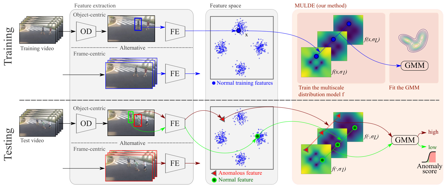
Figure 1. MULDE approximates the negative log-density of noisy, normal video features at multiple levels of noise $\sigma$ with a neural network $f(\cdot,\sigma)$ . The log-likelihoods estimated at multiple noise levels are combined into a single anomaly score with a Gaussian mixture model (GMM). MULDE can be trained to detect video anomalies in an object-centric or frame-centric manner. In the object-centric approach, an object detector (OD) is used to detect objects which are then fed to the feature extractor (FE). In the frame-centric approach, the feature extractor is applied to short sequences of entire frames.
图 1: MULDE 使用神经网络 $f(\cdot,\sigma)$ 在多个噪声水平 $\sigma$ 下近似含噪正常视频特征的负对数密度。通过高斯混合模型 (GMM) 将多个噪声水平估计的对数似然合并为单一异常分数。MULDE 可采用以对象为中心或以帧为中心的方式进行视频异常检测训练。在以对象为中心的方法中,使用对象检测器 (OD) 检测对象后将其输入特征提取器 (FE) ;在以帧为中心的方法中,特征提取器直接作用于整帧的短序列。
In its basic form, introduced above, our method requires choosing the standard deviation $\sigma$ of the noise injected into the data, also called the noise scale. This choice represents a compromise between making $q$ closer to $p$ for small values of $\sigma$ and extending the support of $q$ to cover more possible anomalies at larger noise levels. To avoid this unwelcome compromise, we do not settle on a single $\sigma$ , but approximate the log-density for a range of noise scales with a neural network $f(\cdot,\sigma)$ , and introduce a regularization term that tends to align the approximations at different scales. At test time, we compute anomaly indicators for a range of noise scales and combine them into a single anomaly score with a Gaussian mixture model, fitted to normal data. Our experiments show that MULDE, the regularized MUltiscale Log-DEnsity approximation, is a very effective video anomaly detector.
在上述基本形式中,我们的方法需要选择注入数据的噪声标准差 $\sigma$ (也称为噪声尺度)。这一选择代表了在小 $\sigma$ 值下使 $q$ 更接近 $p$ 与在较大噪声水平下扩展 $q$ 的支持以覆盖更多潜在异常之间的折衷。为了避免这种不理想的权衡,我们并不固定单一 $\sigma$ 值,而是用神经网络 $f(\cdot,\sigma)$ 近似一组噪声尺度 下的对数密度,并引入一个正则化项来对齐不同尺度的近似结果。测试时,我们计算一组噪声尺度的异常指标,并通过拟合正常数据的高斯混合模型将其组合成单一异常分数。实验表明,经过正则化的多尺度对数密度近似方法 MULDE 是一种非常有效的视频异常检测器。
To summarize, the main contribution of this paper is a novel approach to detecting anomalies from video features with a neural approximation of their log-density function. In technical terms, we propose a modification of multiscale denoising score matching for training anomaly indicators and a new method to regularize this training. Our anomaly detector is simple, mathematically sound, and fast at test time, as inference requires merely extracting the features and forward-propagating them through a neural network and a Gaussian mixture model. Moreover, it is agnostic of the feature vector it consumes on input. Our experiments on the Ped2 [28], Avenue [25], Shanghai Tech [26], UCFCrime [39], and UBnormal [1] data sets demonstrate state-of-the-art performance in anomaly detection both in the object-centric setup, where features are extracted from bounding boxes of detected objects, and in the frame-centric setup, with features computed for entire frames.
总结来说,本文的主要贡献是提出了一种新颖方法,通过神经逼近视频特征的对数密度函数来检测异常。从技术上讲,我们改进了多尺度去噪分数匹配 (multiscale denoising score matching) 用于训练异常指标,并提出了一种新的训练正则化方法。我们的异常检测器结构简单、数学严谨且测试速度快,因为推理过程仅需提取特征并通过神经网络和高斯混合模型 (Gaussian mixture model) 进行前向传播。此外,它对输入的特征向量具有通用性。在 Ped2 [28]、Avenue [25]、Shanghai Tech [26]、UCFCrime [39] 和 UBnormal [1] 数据集上的实验表明,无论是在以物体为中心(从检测到的物体边界框提取特征)还是以帧为中心(对整个帧计算特征)的设置中,我们的方法都实现了最先进的异常检测性能。
2. Related Work
2. 相关工作
VAD was studied in multiple settings: as a one-class classification problem, where no anomalous data is available for training [4–6, 8, 9, 13, 14, 25, 26, 30, 31, 35, 43, 45– 48], as an unsupervised learning task, where anomalies are present in the training set, but it is not known which training videos contain them [48], and as a supervised, or weakly supervised problem, where training labels indicate anomalous video frames, or videos containing anomalies, respectively [1, 39, 48]. We address the first of these settings – we assume the training set is limited to normal videos.
视频异常检测(VAD)的研究存在多种设定:作为单类别分类问题(此时训练集中不含异常数据)[4–6, 8, 9, 13, 14, 25, 26, 30, 31, 35, 43, 45–48];作为无监督学习任务(训练集中存在异常但未标注具体视频)[48];以及作为有监督或弱监督问题(训练标签分别标注异常视频帧或含异常的视频)[1, 39, 48]。本文针对第一种设定展开研究——假设训练集仅包含正常视频。
Existing VAD methods can be categorized as framecentric when they operate on features computed from entire frames or their sequences [1, 39, 43, 45, 48], and objectcentric, if they estimate the abnormality of each bounding box in every frame [2, 9–11, 16, 35, 42], typically using a pre-trained feature extractor. The frame-centric design is more suited for global events, like fires, or smoke, while the object-centric one is oriented at anomalies associated with people or objects, like human falls, or vehicle accidents. In Sec. 4, we show that our method can establish state-of-theart performance with features of either type.
现有的视频异常检测(VAD)方法可分为两类:帧中心式(frame-centric)方法基于整帧或其序列计算特征进行操作[1, 39, 43, 45, 48];目标中心式(object-centric)方法则通过预训练特征提取器评估每帧中各个边界框的异常程度[2, 9–11, 16, 35, 42]。帧中心式设计更适合火灾、烟雾等全局事件,而目标中心式则针对人体跌倒、车辆事故等与人或物体相关的异常。如第4节所示,我们的方法使用任一类型的特征都能实现最先进的性能。
The predominant approach to VAD is to train a deep network to auto-encode normal videos and use the reconstruction error as anomaly indicator [4, 8, 13, 26, 30, 31, 46, 47]. The idea of using the error of a model pre-trained on normal data to detect anomalies was extended from auto-encoding to multiple other tasks, including predicting future frames, or the optical flow [8, 22, 23, 30, 47], inpainting spatiotemporal volumes [10], and solving jigsaw puzzles [2, 42]. This over arching approach is predicated on the assumption that the error is higher for anomalous frames than for normal frames. However, there is no certainty that this assumption holds: it is not well understood under what conditions a neural network fails to perform its task and there is no guarantee that all anomalies make it fail. By contrast, no heuristic assumptions underlie the functioning of MULDE.
视频异常检测(VAD)的主流方法是训练深度网络对正常视频进行自动编码,并将重构误差作为异常指标[4, 8, 13, 26, 30, 31, 46, 47]。这种利用在正常数据上预训练模型的误差来检测异常的思路,已从自动编码扩展到多项其他任务,包括预测未来帧或光流[8, 22, 23, 30, 47]、时空修复[10]以及解决拼图问题[2, 42]。这一总体方法基于一个假设:异常帧的重构误差会高于正常帧。然而该假设并不必然成立:我们尚不清楚神经网络在什么条件下会无法完成任务,也无法保证所有异常都会导致其失效。相比之下,MULDE的运行机制不依赖于任何启发式假设。
The idea of detecting video anomalies by modeling the distribution of normal video features recurs in the literature, but, to date, effective modeling techniques remain elusive. Some methods, like Gaussian mixture models [35], one-class Support Vector Machines [5, 6, 25], or multilinear class if i ers [43], may lack the expressive power needed to reflect the complex and high-dimensional distribution of video features. Adversarial ly trained models [11, 21] offer high expressive power, but cannot guarantee to fully capture the distribution, because parts of the feature space may remain unexplored by the generator-disc rim in at or pair during training. Diffusion models capture data distribution, but their use in VAD consists in generating samples of normal frames [45], or human poses [9], and comparing observed frames or poses to generated ones. This requires multiple diffusion steps and reduces the anomaly measure to a distance between the observation and the sample. Normalizing flows, recently used for detecting anomalies in human pose features [14], are free from these drawbacks as they explicitly approximate the likelihood of the training data. However, their performance decreases in the presence of complex correlations between features [19]. In contrast to these methods, MULDE combines all key ingredients of a VAD approach: high expressive power, the capacity to fully capture the distribution, and to accommodate arbitrary features.
通过建模正常视频特征的分布来检测视频异常的想法在文献中反复出现,但迄今为止,有效的建模技术仍然难以捉摸。一些方法,如高斯混合模型 [35]、单类支持向量机 [5, 6, 25] 或多线性分类器 [43],可能缺乏反映视频特征复杂高维分布所需的表达能力。对抗训练模型 [11, 21] 具有高表达能力,但无法保证完全捕获分布,因为在训练过程中生成器-判别器对可能未探索特征空间的某些部分。扩散模型能捕获数据分布,但它们在视频异常检测 (VAD) 中的应用仅限于生成正常帧样本 [45] 或人体姿态 [9],并将观察到的帧或姿态与生成的样本进行比较。这需要多次扩散步骤,并将异常度量简化为观测值与样本之间的距离。最近用于检测人体姿态特征异常的归一化流 [14] 避免了这些缺点,因为它们显式地近似训练数据的似然。然而,当特征之间存在复杂相关性时,其性能会下降 [19]。与这些方法不同,MULDE 结合了视频异常检测方法的所有关键要素:高表达能力、完全捕获分布的能力以及适应任意特征的能力。
The log-density approximation $f$ , employed by MULDE to model the distribution of normal data, is often called the energy, in reference to the energy-based models [20], which represent probability distributions in the Boltzmann form $\begin{array}{r}{q(\bar{x})=\frac{1}{Z}e^{-f(x)}}\end{array}$ , but restrict the model to the energy function $f$ , since computing the normalization constant $Z$ is typically infeasible. MULDE can therefore be seen as an energy-based model. For training $f$ , MULDE relies on a modification of denoising score matching [41], a method to train a neural network to approximate the energy gradient. Score matching models the distribution of the training data injected with iid Gaussian noise, and Song and Ermon [38] extended it to multiple noise levels. Mahmood et al. [29] used the norm of this multi-level energy gradient approximation to detect anomalies in images. However, the gradient indicates all stationary points of the log-density function, which may appear both at the modes of the distribution, where normal data is concentrated, and in low-density regions, where anomalous data may reside. As shown in Fig. 2, some minima and maxima of the distribution remain indistinguishable even across a range of noise scales. By contrast, MULDE approximates the log-density function which, unlike its gradient, is a good anomaly indicator.
MULDE 用于建模正常数据分布的对数密度近似 $f$ 通常被称为能量 (energy) ,这是基于能量模型 [20] 的概念。这些模型以玻尔兹曼形式表示概率分布 $\begin{array}{r}{q(\bar{x})=\frac{1}{Z}e^{-f(x)}}\end{array}$ ,但将模型限制在能量函数 $f$ 上,因为计算归一化常数 $Z$ 通常不可行。因此,MULDE 可被视为一种基于能量的模型。
为了训练 $f$ ,MULDE 采用了去噪分数匹配 [41] 的改进方法,该方法通过训练神经网络来近似能量梯度。分数匹配对注入独立同分布高斯噪声的训练数据分布进行建模,而 Song 和 Ermon [38] 将其扩展到多个噪声级别。Mahmood 等人 [29] 利用这种多级能量梯度近似的范数来检测图像中的异常。然而,梯度仅指示对数密度函数的所有驻点,这些点可能出现在分布模态(正常数据集中区域)或低密度区域(异常数据可能存在的区域)。如图 2 所示,即使在不同噪声尺度下,分布的某些极小值和极大值仍难以区分。相比之下,MULDE 直接近似对数密度函数,与梯度不同,它是一个更好的异常指标。
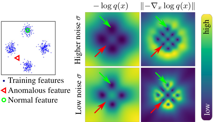
Figure 2. The log-density function is well suited for indicating anomalies, but its gradient is not. (Left:) A sample from a mixture of 4 Gaussians. (Right:) Learned negative log-density approximation (left column) and the norm of its gradient (right column). The negative log-density is a good anomaly indicator, taking low values for normal data and higher values for anomalous data. By contrast, the log-gradient norm is low not only at the modes of the distribution, but also at its minima between the modes, making it impossible to distinguish some anomalies from normal data.
图 2: 对数密度函数适合用于指示异常,但其梯度并不适用。(左图:) 来自4个高斯混合分布的样本。(右图:) 学习到的负对数密度近似(左列)及其梯度范数(右列)。负对数密度是一个良好的异常指标,对正常数据取值较低而对异常数据取值较高。相比之下,对数梯度范数不仅在分布的众数处较低,在众数之间的极小值处也较低,导致无法区分某些异常与正常数据。
3. Method
3. 方法
We perform anomaly detection in the space of semantic features extracted from videos. This lets us focus on detecting semantic anomalies, for example, unusual actions involving objects observed also under normal conditions, as opposed to anomalies in the space of raw input, like frame sequences that do not resemble real videos. We delegate feature extraction to off-the-shelf models and focus on the effective detection of anomalous events that they encode.
我们在从视频中提取的语义特征空间进行异常检测。这种方法让我们专注于检测语义层面的异常,例如在正常条件下也能观察到的物体涉及的不寻常动作,而非原始输入空间中的异常(如与现实视频不符的帧序列)。我们将特征提取任务交由现成模型完成,重点在于有效检测这些模型编码的异常事件。
Motivation Intuitively, anomalous video features should not be observed under ‘normal’ conditions. More formally, an anomalous feature is characterized by a small likelihood under the assumed statistical model of anomaly-free video features. This suggests an approach to detecting anomalies by approximating the probability density function $p$ and simply declaring test features with sufficiently low probability anomalous. We adopt this approach and model the probability density with a neural network.
动机 直观上,在"正常"条件下不应观察到异常视频特征。更正式地说,异常特征的特点是在假设的无异常视频特征统计模型中具有较小的似然性。这表明可以通过近似概率密度函数$p$来检测异常,并简单地声明概率足够低的测试特征为异常。我们采用这种方法,并用神经网络对概率密度进行建模。
Overview In practice, it is difficult to train a neural network to directly approximate the probability density of its training data $p$ . However, injecting the data with noise makes this approximation feasible, as we will explain below. The distribution of the noisy data takes the form
概述
在实践中,很难训练神经网络直接近似其训练数据的概率密度 $p$ 。然而,为数据注入噪声使得这种近似变得可行,我们将在下文解释。噪声数据的分布形式为
$$
q(\tilde{\mathbf{x}})=\int\rho(\tilde{\mathbf{x}}|\mathbf{x})p(\mathbf{x})d\mathbf{x},
$$
$$
q(\tilde{\mathbf{x}})=\int\rho(\tilde{\mathbf{x}}|\mathbf{x})p(\mathbf{x})d\mathbf{x},
$$
where $\rho(\ensuremath{\widetilde{\mathbf{x}}}|\ensuremath{\mathbf{x}})$ denotes the conditional distribution of a noisy sample $\tilde{\bf x}$ given a noise-free sample $\mathbf{x}$ , which we take to be an iid Gaussian centered at $\mathbf{x}$ . The main idea behind our anomaly detector is that $q$ preserves the shape of $p$ but, in contrast to it, yields itself to a neural approximation. Specifically, we approximate, up to a constant, the negative logdensity function $-\log q(\tilde{\mathbf{x}})$ , which is an excellent anomaly indicator due to its bijective relation to $q(\tilde{\mathbf{x}})$ . Low values of $-\log q(\tilde{\mathbf{x}})$ correspond to high probability density and are characteristic of normal data. Its high values indicate areas of low probability density where anomalous data may reside. Fig. 2 illustrates this on a synthetic example. The technique we use to approximate the log-density with a neural network is a modification of score matching [41], a method to approximate the log-density gradient.
其中 $\rho(\ensuremath{\widetilde{\mathbf{x}}}|\ensuremath{\mathbf{x}})$ 表示给定无噪声样本 $\mathbf{x}$ 时噪声样本 $\tilde{\bf x}$ 的条件分布,我们假设其为以 $\mathbf{x}$ 为中心的独立同分布高斯分布。我们异常检测器的核心思想是 $q$ 保留了 $p$ 的形态,但与之不同的是,它可以通过神经网络进行近似。具体来说,我们近似负对数密度函数 $-\log q(\tilde{\mathbf{x}})$(相差一个常数),由于其与 $q(\tilde{\mathbf{x}})$ 的双射关系,这是一个极佳的异常指标。$-\log q(\tilde{\mathbf{x}})$ 的低值对应于高概率密度,是正常数据的特征;其高值则表明低概率密度区域,可能是异常数据所在之处。图 2 在一个合成示例中展示了这一点。我们用于通过神经网络近似对数密度的技术是对分数匹配 [41](一种近似对数密度梯度的方法)的改进。
We introduce score matching in Sec. 3.1 and our training method in Sec. 3.2. In Sec. 3.3 and 3.4, we extend this method to approximating the negative log-density at different scales of injected noise, and introduce a regular iz ation term intended to facilitate combining the multi-scale approxima t ions. We discuss the choice of video features in Sec. 3.5. A diagram of our approach is presented in Fig. 1.
我们在第3.1节介绍分数匹配方法,并在第3.2节阐述训练方法。第3.3和3.4节将该方法扩展到不同噪声尺度下的负对数密度近似,并引入正则化项以促进多尺度近似的结合。第3.5节讨论视频特征的选择。图1展示了本方法的框架示意图。
3.1. Background: Denoising score matching
3.1. 背景:去噪分数匹配
Vincent [41] proposed a method to train a neural network $s$ , parameterized with a vector $\theta$ , to approximate the gradient of the negative log-density function of data perturbed with iid Gaussian noise, in the sense of solving
Vincent [41] 提出了一种训练神经网络 $s$ 的方法,该网络由向量 $\theta$ 参数化,用于近似被独立同分布高斯噪声干扰的数据的负对数密度函数的梯度,其求解目标为
$$
\operatorname*{min}{\theta}\mathbb{E}{\tilde{\mathbf{x}}\sim q(\tilde{\mathbf{x}})}\left|s_{\theta}(\tilde{\mathbf{x}})+\nabla_{\tilde{\mathbf{x}}}\log q(\tilde{\mathbf{x}})\right|_{2}^{2}.
$$
$$
\operatorname*{min}{\theta}\mathbb{E}{\tilde{\mathbf{x}}\sim q(\tilde{\mathbf{x}})}\left|s_{\theta}(\tilde{\mathbf{x}})+\nabla_{\tilde{\mathbf{x}}}\log q(\tilde{\mathbf{x}})\right|_{2}^{2}.
$$
This gradient approximation forms the foundation of a family of generative models [38] which initialize a sample with noise and use the log-gradient approximation to drive the sample close to the mode of the distribution. We will show that it also enables effective detection of video anomalies.
该梯度近似方法构成了一系列生成式模型的基础[38],这些模型通过噪声初始化样本,并利用对数梯度近似驱动样本接近分布模态。我们将证明该方法也能有效检测视频异常。
Directly evaluating the objective (2) is impossible because $q(\tilde{\mathbf{x}})$ is not known analytically, but Vincent [41] showed that it is equivalent, up to a constant, to
直接评估目标函数 (2) 是不可能的,因为 $q(\tilde{\mathbf{x}})$ 无法解析求出,但 Vincent [41] 证明它在常数范围内等价于
$$
\operatorname*{min}{\theta}\mathbb{E}{\tilde{\mathbf{x}}\sim\mathcal{N}(\tilde{\mathbf{x}})}\left|s_{\theta}(\tilde{\mathbf{x}})-\frac{\tilde{\mathbf{x}}-\mathbf{x}}{\sigma^{2}}\right|_{2}^{2},
$$
$$
\operatorname*{min}{\theta}\mathbb{E}{\tilde{\mathbf{x}}\sim\mathcal{N}(\tilde{\mathbf{x}})}\left|s_{\theta}(\tilde{\mathbf{x}})-\frac{\tilde{\mathbf{x}}-\mathbf{x}}{\sigma^{2}}\right|_{2}^{2},
$$
which can be evaluated effectively. This gives rise to a stochastic algorithm for training $s$ that iterates: composing a batch of noise-free training data $\mathbf{x}$ , perturbing it with Gaussian noise to obtain a batch of noisy data $\tilde{\bf x}$ , and making a gradient step on the expectation in Eq. (3), evaluated for the batch. Since this resembles training $s$ to predict the noise injected to $\mathbf{x}$ , it is often called denoising score matching.
这催生了一种用于训练 $s$ 的随机算法,其迭代过程包括:构建一批无噪声训练数据 $\mathbf{x}$,用高斯噪声扰动得到一批含噪数据 $\tilde{\bf x}$,并对式 (3) 中的期望进行梯度下降(基于当前批次计算)。由于这种训练方式类似于让 $s$ 预测注入到 $\mathbf{x}$ 的噪声,因此常被称为去噪分数匹配。
3.2. Anomaly detection by denoising score matching
3.2. 基于去噪分数匹配的异常检测
We modify the denoising score matching formulation to train a neural network $f_{\theta}$ , where $\theta$ denotes the vector of parameters, to approximate $-\log q(\tilde{\mathbf{x}})$ , as opposed to its gradient. To that end, we change the objective (3), to train the gradient of $f$ , instead of the network itself, which yields
我们修改了去噪分数匹配的公式,训练一个神经网络 $f_{\theta}$ (其中 $\theta$ 表示参数向量)来近似 $-\log q(\tilde{\mathbf{x}})$ ,而非其梯度。为此,我们调整了目标函数 (3) ,改为训练 $f$ 的梯度而非网络本身,从而得到
$$
\left.\underset{\vphantom{\int}{\mathrm{ \boldmath~\pi~}}\tilde{\theta}}{\operatorname*{min}}\mathbb{E}{{\bf x}\sim p\left({\bf x}\right)}{\left.\mathbf{x}\sim\mathcal{N}\left(\tilde{\bf x}\right|{\bf x},\sigma{\bf I}\right)}\right|\left|\nabla_{\tilde{\mathbf{x}}}f_{\theta}\left(\tilde{\bf x}\right)-\frac{\tilde{\bf x}-{\bf x}}{\sigma^{2}}\right|_{2}^{2}.
$$
$$
\left.\underset{\vphantom{\int}{\mathrm{ \boldmath~\pi~}}\tilde{\theta}}{\operatorname*{min}}\mathbb{E}{{\bf x}\sim p\left({\bf x}\right)}{\left.\mathbf{x}\sim\mathcal{N}\left(\tilde{\bf x}\right|{\bf x},\sigma{\bf I}\right)}\right|\left|\nabla_{\tilde{\mathbf{x}}}f_{\theta}\left(\tilde{\bf x}\right)-\frac{\tilde{\bf x}-{\bf x}}{\sigma^{2}}\right|_{2}^{2}.
$$
This makes $\nabla_{\tilde{\mathbf{x}}}f_{\theta}\left(\tilde{\mathbf{x}}\right)$ approximate $-\nabla_{\tilde{\mathbf{x}}}\log q(\tilde{\mathbf{x}})$ and, by the fundamental theorem of calculus, aligns $f$ with $-\log q(\tilde{\mathbf{x}})$ up to a constant. Here, $f:\mathbb{R}^{d}\rightarrow\mathbb{R}$ is a mapping from the space of video features to scalar log-density values, and $\nabla_{\tilde{\mathbf{x}}}f_{\theta}:\mathbb{R}^{d}\rightarrow\mathbb{R}^{d}$ , like $s$ in the standard score matching formulation (3), maps $d$ -dimensional video features to $d$ -dimensional vectors of log-density gradients.
这使得 $\nabla_{\tilde{\mathbf{x}}}f_{\theta}\left(\tilde{\mathbf{x}}\right)$ 近似于 $-\nabla_{\tilde{\mathbf{x}}}\log q(\tilde{\mathbf{x}})$ ,并且根据微积分基本定理,将 $f$ 与 $-\log q(\tilde{\mathbf{x}})$ 对齐至一个常数。这里, $f:\mathbb{R}^{d}\rightarrow\mathbb{R}$ 是从视频特征空间到标量对数密度值的映射,而 $\nabla_{\tilde{\mathbf{x}}}f_{\theta}:\mathbb{R}^{d}\rightarrow\mathbb{R}^{d}$ ,如标准分数匹配公式 (3) 中的 $s$ 一样,将 $d$ 维视频特征映射到 $d$ 维对数密度梯度向量。
Notably, our formulation has an advantage over the standard denoising score matching even when the goal is to approximate the gradient of the log-density, as opposed to the log-density itself. By the Stokes’ theorem, gradients form conservative – that is, curl-free – vector fields. Directly approxima ting the log-density gradient with a neural network, as done by the standard approach, may result in a vector field that is not conservative, in other words, does not represent a gradient of any function. By contrast, the gradient of a neural network trained using our formulation is guaranteed to form a conservative vector field. On the downside, training $f_{\theta}$ with our loss requires the network to be twice differentiable, which precludes the use of ReLU, several other nonlinear i ties, and max pooling.
值得注意的是,即使目标是近似对数密度梯度而非对数密度本身,我们的公式也比标准去噪分数匹配更具优势。根据斯托克斯定理,梯度构成保守(即无旋)向量场。标准方法直接使用神经网络近似对数密度梯度,可能导致向量场不保守(即不代表任何函数的梯度)。相比之下,通过我们的公式训练的神经网络梯度,必然构成保守向量场。不足之处在于,使用我们的损失函数训练$f_{\theta}$需要网络具备二阶可微性,这排除了ReLU激活函数、某些其他非线性单元以及最大池化的使用。
3.3. Distribution modeling across noise scales
3.3. 跨噪声尺度的分布建模
We recall that training with our loss (4) makes $f_{\theta}$ approximate the negative log-density of the distribution of noisy data $q(\tilde{\mathbf{x}})$ , connected to the distribution of noise-free data $p(\mathbf{x})$ through the noise distribution $\rho(\ensuremath{\widetilde{\mathbf{x}}}|\ensuremath{\mathbf{x}})$ . $\rho$ is an iid Gaussian centered at $\mathbf{x}$ and with a standard deviation $\sigma$ . The choice of $\sigma$ , called the noise scale, represents a compromise between making $q$ closer to $p$ at small noise scales and extending its support to cover more anomalies for larger noise levels. In theory, the optimal noise scale could be selected by cross-validation on a combination of normal and anomalous data, but in practice, anomalous validation data is rarely available. Therefore, instead of settling for a single noise scale, we approximate the log-density for a range of noise scales and combine the estimates at different scales by modeling their joint distribution with a Gaussian mixture.
我们回顾一下,使用损失函数 (4) 进行训练会使 $f_{\theta}$ 近似于含噪数据分布 $q(\tilde{\mathbf{x}})$ 的负对数密度,该分布通过噪声分布 $\rho(\ensuremath{\widetilde{\mathbf{x}}}|\ensuremath{\mathbf{x}})$ 与无噪数据分布 $p(\mathbf{x})$ 相关联。$\rho$ 是一个以 $\mathbf{x}$ 为中心、标准差为 $\sigma$ 的独立同分布高斯分布。噪声尺度 $\sigma$ 的选择需要在以下两者之间取得平衡:在小噪声尺度下使 $q$ 更接近 $p$,以及在较大噪声水平下扩展其支持范围以覆盖更多异常。理论上,可以通过在正常数据和异常数据组合上进行交叉验证来选择最优噪声尺度,但实际上很少能获得异常验证数据。因此,我们不局限于单一噪声尺度,而是通过高斯混合模型对不同噪声尺度的对数密度估计进行联合建模,从而组合多个尺度下的估计结果。
To implement the multiscale log-density approximation, we take inspiration from Song and Ermon [38], who extended the original score matching formulation, presented in Eq. (3), to multiple noise scales, and apply a similar extension to our objective (4). Instead of approximating $-\log q(\tilde{\mathbf{x}})$ for a fixed $\sigma$ , we approximate a family of functions $-\log q_{\sigma}(\tilde{\mathbf{x}})$ , parameterized by $\sigma$ , with a neural net- work $f_{\theta}$ , conditioned on $\sigma$ . We found it beneficial to put more emphasis on smaller values of $\sigma$ when training $f_{\theta}$ . Thus, we sample $\sigma$ from the log-uniform distribution on the interval $[\sigma_{\mathrm{low}},\sigma_{\mathrm{high}}]$ and minimize
为实现多尺度对数密度近似,我们借鉴了Song和Ermon [38] 的方法,他们将原始分数匹配公式(如式(3)所示)扩展到多噪声尺度,并对我们的目标函数(4)进行了类似扩展。我们不再针对固定σ近似$-\log q(\tilde{\mathbf{x}})$,而是通过神经网络$f_{\theta}$来近似一组由σ参数化的函数$-\log q_{\sigma}(\tilde{\mathbf{x}})$,其中网络以σ为条件。我们发现训练$f_{\theta}$时更关注较小的σ值效果更好。因此,我们从区间$[\sigma_{\mathrm{low}},\sigma_{\mathrm{high}}]$上的对数均匀分布中采样σ并最小化
$$
\left.\begin{array}{l}{\displaystyle\operatorname*{min}{\theta}\mathbb{E}{\mathrm{\boldmath~\scriptstyle{\tilde{\alpha}}~}\sim\mathcal{N}(\tilde{\bf x})}\lambda(\sigma)\left|\nabla_{\tilde{\bf x}}f_{\theta}\left(\tilde{\bf x},\sigma\right)-\frac{\tilde{\bf x}-{\bf x}}{\sigma^{2}}\right|{2}^{2},}\ {\displaystyle\quad\sigma\sim\mathcal{L}\mathcal{U}(\sigma_{\mathrm{low}},\sigma_{\mathrm{high}})}\end{array}\right.
$$
$$
\left.\begin{array}{l}{\displaystyle\operatorname*{min}{\theta}\mathbb{E}{\mathrm{\boldmath~\scriptstyle{\tilde{\alpha}}~}\sim\mathcal{N}(\tilde{\bf x})}\lambda(\sigma)\left|\nabla_{\tilde{\bf x}}f_{\theta}\left(\tilde{\bf x},\sigma\right)-\frac{\tilde{\bf x}-{\bf x}}{\sigma^{2}}\right|{2}^{2},}\ {\displaystyle\quad\sigma\sim\mathcal{L}\mathcal{U}(\sigma_{\mathrm{low}},\sigma_{\mathrm{high}})}\end{array}\right.
$$
where $\lambda(\sigma)$ is a factor that balances the influence of the loss terms at different noise levels. We set $\lambda(\sigma)=\sigma^{2}$ .
其中 $\lambda(\sigma)$ 是平衡不同噪声水平下损失项影响的因子。我们设 $\lambda(\sigma)=\sigma^{2}$。
Once the network is trained, we fit a Gaussian mixture model to multi-scale log-density approximation vectors $[f_{\boldsymbol\theta}(\mathbf{x},\sigma_{i})]{i=1\dots L}$ for an evenly spaced sequence of noise levels ${\sigma_{i}}{i=1}^{L}$ , where ${\sigma_{1}}\mathrm{ =~}\sigma_{\mathrm{{low}}}$ and $\sigma_{L}=\sigma_{\mathrm{high}}$ . At test time, our neural network takes a vector of video features and produces a multi-scale vector of log-density approximations, which is then input to the Gaussian mixture model yielding the final anomaly score.
网络训练完成后,我们对多尺度对数密度近似向量 $[f_{\boldsymbol\theta}(\mathbf{x},\sigma_{i})]{i=1\dots L}$ 拟合高斯混合模型 (Gaussian mixture model),其中噪声水平序列 ${\sigma_{i}}{i=1}^{L}$ 为等间距分布,且满足 ${\sigma_{1}}\mathrm{ =~}\sigma_{\mathrm{{low}}}$ 和 $\sigma_{L}=\sigma_{\mathrm{high}}$。测试阶段,神经网络接收视频特征向量并输出多尺度对数密度近似向量,该向量随后输入高斯混合模型生成最终异常分数。
3.4. Multiscale training regular iz ation
3.4. 多尺度训练正则化
The limitation of our method is that $f_{\boldsymbol{\theta}}(\cdot,\boldsymbol{\sigma})$ can be trained to approximate $-\log q_{\sigma}(\tilde{\mathbf{x}})$ only up to a constant. That is, $f_{\boldsymbol{\theta}}(\tilde{{\mathbf x}},\boldsymbol{\sigma})$ effectively approximates $-\log q_{\sigma}(\tilde{\mathbf{x}})+C_{\sigma}$ , where $C_{\sigma}$ is a constant that we do not know. In our formulation, there is no guarantee that this constant does not change across the range of $\sigma$ . Since the variation of $C_{\sigma}$ may make it more difficult to aggregate the estimates at different scales, we discourage it by using a regular iz ation term $f_{\theta}(\mathbf{x},\sigma)^{2}$ , that penalizes the log-densities of noise-free examples. Our full training objective thus becomes
我们方法的局限性在于 $f_{\boldsymbol{\theta}}(\cdot,\boldsymbol{\sigma})$ 只能训练到近似 $-\log q_{\sigma}(\tilde{\mathbf{x}})$ 加上一个常数。也就是说,$f_{\boldsymbol{\theta}}(\tilde{{\mathbf x}},\boldsymbol{\sigma})$ 实际上近似的是 $-\log q_{\sigma}(\tilde{\mathbf{x}})+C_{\sigma}$,其中 $C_{\sigma}$ 是一个未知常数。在我们的公式中,无法保证这个常数在 $\sigma$ 的取值范围内保持不变。由于 $C_{\sigma}$ 的变化可能会增加不同尺度下估计值聚合的难度,我们通过使用正则化项 $f_{\theta}(\mathbf{x},\sigma)^{2}$ 来抑制这种情况,该正则化项会对无噪声样本的对数密度进行惩罚。因此,我们的完整训练目标变为
$$
\begin{array}{r l}{\underset{\theta}{\mathop{\operatorname*{min}}}\underbrace{{\mathbb{E}}\mathbf{\phi}{\mathbf{x}\sim p(\mathbf{x})}}{\underbrace{\mathbf{\tilde{x}}\sim\mathcal{N}(\tilde{\mathbf{x}}|\mathbf{x},\sigma\mathbf{I})}}\quad\Big[\lambda(\sigma)\left|\nabla_{\tilde{\mathbf{x}}}f_{\theta}\left(\tilde{\mathbf{x}},\sigma\right)-\frac{\tilde{\mathbf{x}}-\mathbf{x}}{\sigma^{2}}\right|{2}^{2}}\ {\qquad\sigma\sim\mathcal{L U}(\sigma_{\mathrm{low}},\sigma_{\mathrm{high}})}\ &{\qquad+\beta f_{\theta}(\mathbf{x},\sigma)^{2}\Big],}\end{array}
$$
$$
\begin{array}{r l}{\underset{\theta}{\mathop{\operatorname*{min}}}\underbrace{{\mathbb{E}}\mathbf{\phi}{\mathbf{x}\sim p(\mathbf{x})}}{\underbrace{\mathbf{\tilde{x}}\sim\mathcal{N}(\tilde{\mathbf{x}}|\mathbf{x},\sigma\mathbf{I})}}\quad\Big[\lambda(\sigma)\left|\nabla_{\tilde{\mathbf{x}}}f_{\theta}\left(\tilde{\mathbf{x}},\sigma\right)-\frac{\tilde{\mathbf{x}}-\mathbf{x}}{\sigma^{2}}\right|{2}^{2}}\ &{\qquad\sigma\sim\mathcal{L U}(\sigma_{\mathrm{low}},\sigma_{\mathrm{high}})}\ {\qquad+\beta f_{\theta}(\mathbf{x},\sigma)^{2}\Big],}\end{array}
$$
where $\beta$ is a hyper parameter of our method. Minimizing (6) no longer makes $\nabla_{\mathbf x}f_{\theta}$ an unbiased estimate of the loggradient of the distribution, but as shown in our ablation studies, it improves our results in video anomaly detection. Algorithm 1 summarizes training the log-density approximation $f_{\theta}$ . The Gaussian mixture model is fitted with the standard expectation-maximization algorithm.
其中 $\beta$ 是我们方法的一个超参数。最小化 (6) 不再使 $\nabla_{\mathbf x}f_{\theta}$ 成为分布对数梯度的无偏估计,但如我们的消融实验所示,它提升了视频异常检测的效果。算法 1 总结了训练对数密度近似 $f_{\theta}$ 的过程。高斯混合模型采用标准期望最大化算法进行拟合。
3.5. Selection of video features
3.5. 视频特征选择
Feature selection is closely tied to the type of target anomalies. For example, human pose features are well suited for detecting falls, and optical-flow-based ones help detect objects moving with unusual speeds or in unusual directions. MULDE is feature agnostic and in Sec. 4 we demonstrate
特征选择与目标异常类型密切相关。例如,人体姿态特征非常适合检测跌倒行为,而基于光流(optical flow)的特征有助于检测以异常速度或方向移动的物体。MULDE具有特征无关性,在第4节我们将展示
Algorithm 1 Training MULDE’s anomaly indicator. The terms and steps that differ from the standard multi-scale denoising score matching [38] are highlighted.
算法 1: 训练 MULDE 的异常指标。与标准多尺度去噪分数匹配 [38] 不同的术语和步骤已高亮标注。
Require:
要求:
针对神经对数密度模型,参数化为θ
训练集T包含正常视频特征
噪声尺度范围下限Olow与上限Ohigh
正则化强度β
1: θ ← 随机初始化
2: while 未收敛 do
3: X ← 从T中采样一个批次
4: for x ∈ X do // 遍历批次元素
5: σ ← 对数均匀采样(Olow, Ohigh)
its application with pose, velocity, and deep features, extracted from bounding boxes of object proposals, and ones extracted from entire frames and their sequences. As reported in Sec. 4, feature extraction dominates the running time of our method, which enables selecting the feature extractor to match the desired frame rate.
其应用包括姿态、速度以及从物体提议的边界框中提取的深度特征,以及从整个帧及其序列中提取的特征。如第4节所述,特征提取在我们的方法中占据了大部分运行时间,这使得可以根据所需的帧率选择合适的特征提取器。
4. Experimental Evaluation
4. 实验评估
Data sets We evaluated MULDE on five VAD benchmarks, containing videos captured with static cameras:
数据集
我们在五个视频异常检测(VAD)基准上评估了MULDE,这些数据集均采用静态摄像头拍摄的视频:
• Ped2 [28] includes 16 training and 12 test videos of a campus scene. The training videos show pedestrians and the test videos contain anomalies, like cyclists, skateboarders, and cars in pedestrian areas. • Avenue [25] consists of 16 training and 21 test videos of a walkway. Anomalies include people running, throwing objects, and walking in the wrong direction. • Shanghai Tech [26] comprises 330 training and 107 test videos of 13 pedestrian traffic scenes differing by the camera viewpoint and lighting conditions. Anomalous events include robbery, jumping, fighting, and cycling. • UBnormal [1] is composed of 543 synthetic videos of 29 virtual scenes. It contains human-related anomalies, like fighting, running, and jumping, but it also includes car accidents and environmental anomalies, like fog. • UCFCrime [39] contains 1900 real-world surveillance videos, totaling 128 hours, and including 13 anomaly types, like fighting, robbery, road accidents, and burglary.
- Ped2 [28] 包含16个训练视频和12个测试视频,场景为校园。训练视频展示行人,测试视频则包含异常行为,如骑行、滑板以及行人区域出现车辆。
- Avenue [25] 由16个训练视频和21个测试视频组成,拍摄于一条人行道。异常行为包括奔跑、投掷物品以及逆向行走。
- Shanghai Tech [26] 包含330个训练视频和107个测试视频,涵盖13个不同摄像头视角与光照条件的行人交通场景。异常事件涉及抢劫、跳跃、斗殴及骑行。
- UBnormal [1] 由543个合成视频构成,覆盖29个虚拟场景。除人类相关异常(如斗殴、奔跑、跳跃)外,还包含车祸及环境异常(如雾气)。
- UCFCrime [39] 包含1900段真实监控视频,总时长128小时,涉及13类异常事件,例如斗殴、抢劫、交通事故和入室盗窃。
All our experiments were run in the ‘one-class classification’ setting, that is, we used no anomalous videos for training. In the experiments on UBnormal and UCFCrime, which contain anomalous training videos, we discarded these videos and restricted training to normal data.
我们的所有实验均在"单类分类"设置下运行,即训练过程中未使用任何异常视频。对于包含异常训练视频的UBnormal和UCFCrime数据集实验,我们弃用这些视频并将训练数据严格限定为正常样本。
Performance metrics We followed the standard practice and gauged performance on a frame-by-frame basis. For the object-centric approaches, which yield an anomaly score for each object detected in every frame, we took the highest, i.e. most anomalous, score in a frame for the evaluation. We used the area under the receiver operating characteristic curve (AUC-ROC) as the main performance metric.
性能指标
我们遵循标准做法,逐帧评估性能。对于以物体为中心的方法,这些方法会为每帧中检测到的每个物体生成一个异常分数,我们取帧中最高的(即最异常的)分数进行评估。我们使用接收者操作特征曲线下面积 (AUC-ROC) 作为主要性能指标。
Two methods to aggregate the AUC-ROC over multiple videos can be found in the literature: the micro and the macro score [1, 2, 11, 35, 36]. For the macro score, the AUC-ROC is computed separately for each video and then averaged across all videos in the test set. The micro score computes the AUC-ROC jointly for all frames of all test videos. In abstract terms, the macro score reflects performance attained by adjusting the detection threshold for each video independently, and the micro score is more conservative and applies the same threshold to all test videos. Since we address a VAD use case without an adaptive threshold, we rely on the micro score in our evaluation, but report the results in terms of both metrics. In the supplementary material, we additionally report the tracking- and region-based metrics by Rama chandra and Jones [33].
文献中记载了两种聚合多视频AUC-ROC的方法:微观分数(micro score)和宏观分数(macro score) [1, 2, 11, 35, 36]。宏观分数会为每个视频单独计算AUC-ROC,然后对测试集中所有视频的结果取平均值。微观分数则联合计算所有测试视频帧的AUC-ROC。抽象地说,宏观分数反映了通过为每个视频独立调整检测阈值所获得的性能,而微观分数更为保守,对所有测试视频应用相同的阈值。由于我们处理的视频异常检测(VAD)用例没有自适应阈值,因此在评估中采用微观分数,但会同时报告两种指标的结果。在补充材料中,我们还额外报告了Rama chandra和Jones [33]提出的基于跟踪和区域的指标。
Baselines We compared MULDE to the best-performing VAD algorithms, including ones based on the reconstruction error [10, 16, 47], auxiliary tasks [1, 2, 10, 24, 36, 42, 45], adversarial training [1, 8, 11, 48], normalizing flows [14], and one-class classification with a multi linear classifier [43]. We reproduced the performance metrics of these methods as reported in the original papers. We present an even broader comparison, including less recent work, in the supplementary material.
基线方法
我们将MULDE与性能最佳的语音活动检测(VAD)算法进行了比较,包括基于重构误差的方法 [10, 16, 47]、基于辅助任务的方法 [1, 2, 10, 24, 36, 42, 45]、基于对抗训练的方法 [1, 8, 11, 48]、基于标准化流的方法 [14] 以及使用多线性分类器的单类分类方法 [43]。我们按照原始论文报告的性能指标复现了这些方法的结果。补充材料中还提供了更广泛的比较,包括一些较早的研究工作。
Two baselines are related to our method more closely than the others. The AccI-VAD [35] approximates the probability density function of normal video features with a Gaussian mixture model, while we perform this approximation with a neural network. MSMA [29] uses the norm of the log-density gradient as an anomaly indicator, while our anomaly indicator is based on the log-density itself. Since MSMA was developed for image anomaly detection, we reimplemented it to work with video features.
有两种基线方法与我们的方法关联更为密切。AccI-VAD [35] 采用高斯混合模型近似正常视频特征的概率密度函数,而我们使用神经网络进行这种近似。MSMA [29] 使用对数密度梯度的范数作为异常指标,而我们的异常指标基于对数密度本身。由于 MSMA 是为图像异常检测开发的,我们重新实现了它以处理视频特征。
Implementation details In our experiments, our density model $f_{\theta}$ para met rize d by $\theta$ has two hidden layers with 4096 units followed by GELU nonlinear i ties. The final layer has an output dimension of one without any nonlinearity. It is trained using the Adam update rule [18], with exponential decay rates $\beta_{1}=0.5$ and $\beta_{2}=0.9$ , and a batch size of 2048. We use the learning rates of 5e-4 and 1e-4 in the object- and frame-centric experiments, respectively.
实现细节
在我们的实验中,密度模型 $f_{\theta}$ (参数化为 $\theta$) 包含两个隐藏层,每层有4096个单元,后接GELU非线性激活。最后一层输出维度为1且不包含任何非线性。模型使用Adam更新规则 [18] 进行训练,指数衰减率 $\beta_{1}=0.5$ 和 $\beta_{2}=0.9$,批量大小为2048。在物体中心实验和帧中心实验中,我们分别使用5e-4和1e-4的学习率。
Table 1. Object-centric results. Frame-level AUC-ROC $(%)$ comparison (best marked bold, second best underlined). *implemented by us.
表 1. 以对象为中心的结果。帧级AUC-ROC $(%)$ 对比 (最优值加粗显示,次优值加下划线)。*由我们实现。
| 方法 | Ped2 | Avenue | ShanghaiTech | |||
|---|---|---|---|---|---|---|
| Micro | Macro | Micro | Macro | Micro | Macro | |
| CAE-SVM[16] | 94.3 | 97.8 | 87.4 | 90.4 | 78.7 | 84.9 |
| VEC [47] | 97.3 | 90.2 | 74.8 | |||
| SSMTL [10] | 97.5 | 99.8 | 91.5 | 91.9 | 82.4 | 89.3 |
| HF2 [24] | 99.3 | 91.1 | 93.5 | 76.2 | ||
| BA-AED [11] | 98.7 | 99.7 | 92.3 | 90.4 | 82.7 | 89.3 |
| [11]+SSPCAB[36] | 92.9 | 91.9 | 83.6 | 89.5 | ||
| Jigsaw-Puzzle[42] | 99.0 | 99.9 | 92.2 | 93.0 | 84.3 | 89.8 |
| [10]+UbNormal[1] | 93.0 | 93.2 | 83.7 | 90.5 | ||
| AccI-VAD[35] | 99.1 | 99.9 | 93.3 | 96.2 | 85.9 | 89.6 |
| SSMTL++ [2] | 93.7 | 92.5 | 83.8 | 90.5 | ||
| MSMA*[29] | 99.5 | 99.9 | 90.2 | 92.5 | 84.1 | 90.2 |
| STG-NF [14] | 85.9 | |||||
| MULDE3=0 (ours) | 99.7 | 99.9 | 93.1 | 96.1 | 86.4 | 91.0 |
| MULDE (ours) | 99.7 | 99.9 | 94.3 | 96.1 | 86.7 | 91.5 |
Both during training and at test time, we standardize the video features component-wise using the statistics of the training set. During training, we sample the noise scale used for each batch element from the log-uniform distribution on the interval $[\sigma_{\mathrm{low}},\sigma_{\mathrm{high}}]=[1\mathrm{e}{-}3,1.0]$ . For evaluation, we use $L=16$ evenly spaced noise levels between $[\sigma_{\mathrm{low}},\sigma_{\mathrm{high}}]$ .
在训练和测试期间,我们使用训练集的统计数据对视频特征进行逐分量标准化。训练时,我们从区间 $[\sigma_{\mathrm{low}},\sigma_{\mathrm{high}}]=[1\mathrm{e}{-}3,1.0]$ 的对数均匀分布中为每批元素采样噪声尺度。评估时,我们在 $[\sigma_{\mathrm{low}},\sigma_{\mathrm{high}}]$ 之间使用 $L=16$ 个均匀间隔的噪声级别。
Video feature extraction MULDE is agnostic of the features used to represent the video content. In our experiments, we reused off-the-shelf video feature extractors.
视频特征提取
MULDE 不限定用于表示视频内容的特征类型。在我们的实验中,我们复用了现成的视频特征提取器。
In the object-centric experiments, we used the feature extraction pipeline proposed by Reiss and Hoshen [35]. It detects objects in each video frame and extracts deep and velocity features for each detected object. Additionally, pose features are extracted for each detected person. The pose vector contains coordinates of 17 keypoints and is obtained with AlphaPose [7]. CLIP image encoder [32] is used to extract deep features, which take the form of 512-dimensional vectors. The velocity features are produced by FlowNet 2.0 [15] and binned into histograms of oriented flows.
在以物体为中心的实验中,我们采用了Reiss和Hoshen [35]提出的特征提取流程。该流程检测每帧视频中的物体,并为每个检测到的物体提取深度特征和速度特征。此外,还会为每个检测到的人体提取姿态特征。姿态向量包含17个关键点的坐标,通过AlphaPose [7]获得。CLIP图像编码器 [32]用于提取深度特征,这些特征以512维向量的形式呈现。速度特征由FlowNet 2.0 [15]生成,并被分箱为定向流直方图。
In the frame-centric experiments, we extracted features using Hiera-L [37], a masked auto encoder pre-trained on images and fine-tuned on Kinetics 400 [17], a largescale video action recognition data set. Hiera-L takes sequences of 16 frames as input and produces feature 1152- dimensional feature vectors.
在帧中心实验中,我们使用Hiera-L [37]提取特征,这是一种在图像上预训练并在Kinetics 400 [17](一个大规模视频动作识别数据集)上微调的掩码自编码器。Hiera-L以16帧序列作为输入,并生成1152维特征向量。
Performance in object-centric VAD We present the results in object-centric VAD in Table 1. MULDE outperforms all the baselines in terms of the more conservative micro score. Interestingly, AccI-VAD which, like MULDE, relies on modeling the probability density of normal data, ranks third on all three data sets. The high accuracy of both methods speaks in favor of the density modeling approach, while the edge MULDE holds over AccI-VAD attests to the superiority of MULDE’s neural density model over the combination of Gaussian mixture models and the $\mathbf{k}\mathbf{\cdot}$ -th nearest neighbor technique employed by AccI-VAD. MSMA, which uses an approximation of the log-density gradient as anomaly indicator, is outperformed by our logdensity-based method by a fair margin.
以目标为中心的视频异常检测性能
我们在表1中展示了以目标为中心的视频异常检测(VAD)结果。MULDE在更为保守的微观评分指标上超越了所有基线方法。值得注意的是,与MULDE类似、同样基于正常数据概率密度建模的AccI-VAD,在三个数据集中均位列第三。两种方法的高准确率印证了密度建模方法的有效性,而MULDE对AccI-VAD的优势则证明了其神经密度模型优于后者采用的高斯混合模型与$\mathbf{k}\mathbf{\cdot}$近邻技术组合的方案。使用对数密度梯度近似作为异常指标的MSMA方法,其表现显著逊于我们基于对数密度的方法。
Table 2. Frame-centric results. Frame-level AUC-ROC $(%)$ comparison (best marked bold, second best underlined). *implemented by us.
表 2. 帧中心结果。帧级 AUC-ROC $(%)$ 比较 (最佳加粗,次佳加下划线)。*由我们实现。
| 方法 | ShanghaiTech | UCF-Crime | UBnormal | |||
|---|---|---|---|---|---|---|
| Micro | Macro | Micro | Macro | Micro | Macro | |
| CT-D2GAN[8] | 77.7 | |||||
| CAC [44] | 79.3 | |||||
| Scene-Aware[40] | 74.7 | 72.7 | ||||
| GODS [43] | 70.5 | |||||
| GCL [48] | 74.2 | |||||
| UBnormal [1] | 68.5 | 80.3 | ||||
| FPDM [45] | 78.6 | 74.7 | 62.7 | |||
| AccI-VADGMM* [35] | 76.2 | 82.9 | 60.3 | 84.5 | 66.8 | 83.2 |
| AccI-VADkNN*[35] | 71.9 | 83.1 | 53.0 | 82.7 | 65.2 | 82.5 |
| MSMA*[29] | 76.7 | 84.2 | 64.5 | 83.4 | 70.3 | 85.1 |
| MULDEg=o(ours) | 78.4 | 86.0 | 75.9 | 84.8 | 71.3 | 86.0 |
| MULDE(ours) | 81.3 | 85.9 | 78.5 | 84.9 | 72.8 | 85.5 |
Performance in frame-centric VAD As can be seen in Table 2, in frame-centric VAD, MULDE outperforms other methods on all three data sets. Notably, on the UCFCrime data set, by far the largest publicly available VAD benchmark, we advance the state of the art in terms of the micro score by 3.8 percent points. We improve the state of the art by more than 2pp on Shanghai Tech and UBnormal.
帧中心VAD性能表现
如表2所示,在帧中心VAD任务中,MULDE方法在三个数据集上均优于其他方法。值得注意的是,在当前最大的公开VAD基准数据集UCFCrime上,我们将微观分数指标提升了3.8个百分点。在Shanghai Tech和UBnormal数据集上,我们的方法也将当前最优结果提高了超过2个百分点。
Moreover, while recent object-centric methods dominate frame-centric methods on data sets enabling both types of evaluation, MULDE narrows this performance gap, attaining the micro score of $81.3%$ in frame-centric VAD on Shanghai Tech and $86.7%$ in object-centric VAD on the same data set. On UBnormal, our frame-centric approach even outperforms the object-centric state-of-the-art method [14] by 1.1 percent points of the micro score.
此外,尽管近期以物体为中心的方法在支持两种评估类型的数据集上优于以帧为中心的方法,但MULDE缩小了这一性能差距,在上海科技大学数据集上以帧为中心的异常检测(VAD)中取得了81.3%的微平均分数,在同一数据集上以物体为中心的VAD中达到86.7%。在UBnormal数据集上,我们的帧中心方法甚至以1.1个百分点的微平均分数优势超越了当前最先进的物体中心方法[14]。
Ablation studies To validate the design of MULDE, we run ablation studies and evaluated the contribution to performance from our regular iz ation term, the Gaussian mixture model, and the architecture of our anomaly indicator.
消融实验
为验证 MULDE 的设计,我们进行了消融实验,评估了正则化项、高斯混合模型以及异常指标架构对性能的贡献。
As shown in Table 3, regular iz ation improves the results of frame-centric VAD in terms of the micro score, although different values of the regular iz ation factor $\beta$ are optimal for different data sets. We take $\beta=0.1$ as a compromise among performance on the three data sets. A qualitative example of anomaly detection by MULDE with and without regular iz ation, shown in Fig. 3, demonstrates that a regularized model produces stronger anomaly indications.
如表 3 所示,正则化 (regularization) 在微观分数 (micro score) 方面提升了帧中心语音活动检测 (frame-centric VAD) 的结果,尽管不同的正则化因子 $\beta$ 值对不同数据集效果最佳。我们选择 $\beta=0.1$ 作为在三个数据集性能之间的折衷方案。图 3 展示了 MULDE 在有/无正则化情况下的异常检测定性示例,表明经过正则化的模型能产生更显著的异常指示。
Table 3. Frame-centric performance of MULDE trained with different values of the regular iz ation parameter $\beta$ . Frame-level AUCROC $(%)$ comparison (best marked bold, second best underlined).
表 3: 采用不同正则化参数 $\beta$ 训练的 MULDE 帧中心性能。帧级 AUCROC $(%)$ 对比 (最优值加粗,次优值加下划线)。
| β | ShanghaiTech | UCF-Crime | UBnormal | |||
|---|---|---|---|---|---|---|
| Micro | Macro | Micro | Macro | Micro | Macro | |
| 0.0 | 78.4 | 86.0 | 75.9 | 84.8 | 71.3 | 86.0 |
| 0.01 | 80.7 | 84.9 | 76.6 | 84.9 | 72.9 | 85.2 |
| 0.1 | 81.3 | 85.9 | 78.5 | 84.9 | 72.8 | 85.5 |
| 1.0 | 81.4 | 84.5 | 77.2 | 85.5 | 72.5 | 84.7 |
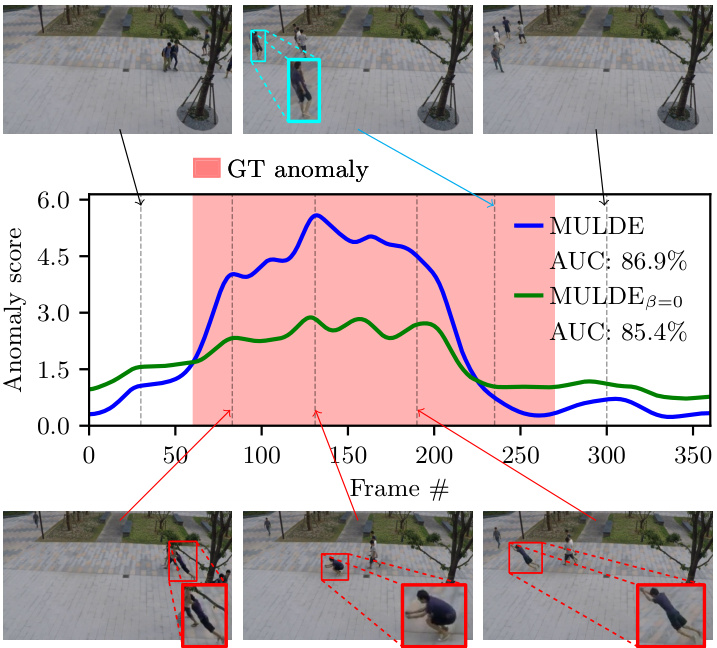
Figure 3. Anomaly detection with MULDE in a test video of the Shanghai Tech data set (video 13 in scene 4). Pedestrians walking in frames 30 and 300 represent normal behavior. A person jumping across the scene is annotated as anomalous. The anomaly indication produced by MULDE is aligned with the ground truth (GT) at its beginning but terminates earlier than the GT annotation. However, careful examination of the video reveals that normal behavior (walking, cyan bounding box in the top row) is re-instantiated before the end of the annotation, as indicated by MULDE. A regularized model produces a stronger anomaly indication (plotted in blue) than one without regular iz ation (green plot).
图 3: 使用 MULDE 在上海科技大学数据集的测试视频 (场景4中的视频13) 中进行异常检测。第30帧和第300帧中行人行走属于正常行为。跨越场景跳跃的人被标注为异常。MULDE生成的异常指示在开始时与真实标注 (GT) 对齐,但比GT标注提前结束。不过仔细观察视频可以发现,在标注结束前已恢复为正常行为 (行走,顶部青色边界框),这与MULDE的检测结果一致。经过正则化的模型 (蓝色曲线) 比未正则化的模型 (绿色曲线) 产生了更强的异常指示信号。
As explained in Section 3.3, MULDE combines anomaly indications computed for a range of noise scales with a Gaussian mixture model fitted to normal data. This lets us avoid the need to select the noise scale to be used at test time. Fig. 4 demonstrates the impact of the mixture model on performance. It shows the micro score attained by our anomaly indicator $f_{\boldsymbol{\theta}}(\cdot,\boldsymbol{\sigma})$ at individual noise scales, without the mixture model. The best performance is attained for intermediate levels of noise, which suggests a tradeoff between representing the noise-free distribution more faith
如第3.3节所述,MULDE通过将针对多组噪声尺度计算的异常指标与拟合正常数据的高斯混合模型相结合,从而避免在测试时选择特定噪声尺度。图4展示了混合模型对性能的影响:图中显示我们的异常指标$f_{\boldsymbol{\theta}}(\cdot,\boldsymbol{\sigma})$在未使用混合模型时,于各独立噪声尺度上取得的微观分数。最佳性能出现在中等噪声水平,这表明在更忠实表征无噪声分布与...之间存在权衡。

Figure 4. Performance of MULDE in frame-centric VAD on the Shanghai Tech data set without the Gaussian mixture model, with our anomaly indicator computed at individual noise scales (blue plot), and with the mixture model with 1, 3, and 5 components.
图 4: MULDE 在上海科技大学数据集上进行帧中心视频异常检测(VAD)的性能表现:(a) 未使用高斯混合模型(GMM);(b) 使用我们在单个噪声尺度上计算得到的异常指标(蓝色曲线);(c) 使用包含1、3、5个分量的混合模型。
| 单元数 | 1层 | 2层 | 3层 | 4层 | ||||
|---|---|---|---|---|---|---|---|---|
| Micro | MacroMicro | Macro | Micro | Macro | Micro | Macro | ||
| 1024 | 77.3 | 84.2 | 79.9 | 85.4 | 81.2 | 85.8 | 79.9 | 84.2 |
| 2048 | 77.6 | 84.6 | 80.4 | 84.6 | 79.2 | 83.5 | 79.4 | 84.0 |
| 4096 | 78.4 | 84.6 | 81.3 | 85.9 | 79.5 | 84.4 | 80.0 | 84.2 |
| 8192 | 79.2 | 84.3 | 79.4 | 84.8 | 80.4 | 84.4 | 79.3 | 84.7 |
Table 4. Performance of MULDE with architectural variations in frame-centric VAD on Shanghai Tech. Units indicate the number of neurons within a hidden layer. Columns correspond to the number of hidden layers. Frame-level AUC-ROC $(%)$ comparison (best marked bold, second best underlined).
表 4: 上海科技大学数据集上帧中心VAD架构变体的MULDE性能。单位表示隐藏层中的神经元数量。列对应隐藏层数量。帧级AUC-ROC (%) 比较 (最佳加粗标记,次佳加下划线)。
fully at lower noise scales and better covering the space away from training examples at higher noise scales. Performance attained with the mixture model slightly exceeds the one attained with the optimal noise scale, validating the GMM as a method to avoid tuning the noise level.
在较低噪声尺度下完全覆盖,在较高噪声尺度下更好地覆盖远离训练样本的空间。混合模型达到的性能略优于最优噪声尺度下的表现,验证了高斯混合模型 (GMM) 作为避免调整噪声水平方法的有效性。
To find the optimal architecture of our anomaly indicator $f_{\theta}$ , we performed an ablation study over the number of hidden layers and the number of neurons in each hidden layer. The results, presented in Table 4, suggest the optimal depth of two hidden layers and the width of 4096 neurons, which we used in our experiments.
为确定异常指标 $f_{\theta}$ 的最优架构,我们对隐藏层数量和每层神经元数量进行了消融实验。表4所示结果表明:采用2个隐藏层、每层4096个神经元的架构效果最佳,该配置已应用于后续实验。
Running time Once a feature has been extracted from the video, MULDE requires only a forward-pass through the shallow network $f_{\theta}$ and an evaluation of a Gaussian mixture model. This represents a very small computational overhead over feature extraction. In the frame-centric approach with 512-dimensional feature vectors, MULDE takes less than one millisecond to process a single feature. For comparison, the Hiera-L feature extractor [37], used in the frame-centric experiments, requires 130 milliseconds to compute one feature vector from a sequence of 16 frames. MULDE’s running time is therefore dominated by the time needed for feature extraction, which means that the feature extractor can be selected to match the target framerate on a given architecture. For example, in our setup, extracting a single feature with the smaller Hiera-base model takes 33 milliseconds, which enables video anomaly detection at 25 FPS, even on our PC with an NVIDIA RTX 2080Ti GPU.
运行时间
一旦从视频中提取出特征,MULDE仅需通过浅层网络 $f_{\theta}$ 进行一次前向传播,并评估一个高斯混合模型。这相对于特征提取过程仅带来极小的计算开销。在使用512维特征向量的帧中心化方法中,MULDE处理单个特征耗时不足1毫秒。作为对比,帧中心化实验采用的Hiera-L特征提取器[37]需要130毫秒才能从16帧序列计算出一个特征向量。因此,MULDE的运行时间主要取决于特征提取所需时长,这意味着可以根据目标帧率选择适配特定架构的特征提取器。例如,在我们的配置中,使用更小的Hiera-base模型提取单个特征耗时33毫秒,这使得即使在配备NVIDIA RTX 2080Ti GPU的PC上也能实现25 FPS的视频异常检测。
5. Discussion
5. 讨论
Limitations Our method has two main limitations. First, our video anomaly detector requires features of anomalous and normal videos to be distinguishable. Intuitively, this condition should be satisfied when the video feature extractor is selected adequately, but there is no theoretical guarantee that this is indeed the case. Second, even though our method eliminates the need to select the noise scale used for training, the range of employed noise scales should be sufficiently large to cover anomalies that would be seen at test time. Currently, there is no automatic way to select the upper limit of the noise range. We circumvent this limitation by standardizing the features component-wise and using a fixed, wide range of noise scales.
限制
我们的方法存在两个主要局限性。首先,视频异常检测器要求异常视频与正常视频的特征可区分。直观来看,当视频特征提取器选择适当时该条件应被满足,但理论上无法保证必然成立。其次,尽管本方法无需选择训练所用的噪声尺度,但所采用的噪声尺度范围仍需足够大以覆盖测试时可能出现的异常。目前尚无自动选择噪声范围上限的方法,我们通过对特征进行分量标准化并使用固定宽幅噪声尺度来规避这一限制。
Future work We plan to extend this work by exploring architectures of the video anomaly indicator. In particular, reformulating the anomaly indicator in terms of the reconstruction error [10–13, 16, 31] represents a distinct opportunity to integrate previous methods into our approach.
未来工作
我们计划通过探索视频异常指标的架构来扩展这项工作。特别是,基于重构误差 [10–13, 16, 31] 重新定义异常指标,为将先前方法整合到我们的方案中提供了独特机遇。
Our method uses Gaussian noise during training, but other forms of noise may represent anomalies more effectively. For example, emulating random motion patterns in the video might be useful for detecting objects moving along unusual trajectories or with abnormal velocities.
我们的方法在训练过程中使用高斯噪声 (Gaussian noise) ,但其他形式的噪声可能更有效地表示异常。例如,模拟视频中的随机运动模式可能有助于检测沿异常轨迹移动或以异常速度运动的物体。
Finally, we plan to extend MULDE from the one-classclassification scenario to the (weakly-) supervised one.
最后,我们计划将 MULDE 从单分类场景扩展到(弱)监督场景。
Conclusion We presented a novel approach to video anomaly detection by modeling the distribution of nonanomalous video features with a neural network. Our method is fast and attains state-of-the-art performance, both in the frame-centric and object-centric VAD. Most importantly, it is firmly grounded in statistical modeling. We defined abnormality in terms of the probability density under the distribution of normal data and designed MULDE to approximate the log-density function. This lets us discuss our method in statistical terms. For example, when our anomaly indicator fails to classify a video as anomalous, we know that its log-density approximation is not good enough. We can then plan actions to rectify this, for example, by changing the neural network architecture, acquiring more training data, or modifying the range of noise. By contrast, it might not be obvious what actions should be taken when previous methods fail, for example, by showing a small reconstruction error for an anomalous item.
结论
我们提出了一种新颖的视频异常检测方法,通过神经网络建模正常视频特征的分布。该方法在帧中心和物体中心的视频异常检测(VAD)中均实现了快速且最先进的性能。最重要的是,该方法严格建立在统计建模的基础上。我们基于正常数据分布下的概率密度定义了异常性,并设计了MULDE来近似对数密度函数。这使得我们能够从统计学角度讨论该方法。例如,当我们的异常指标未能将视频分类为异常时,我们知道其对数密度近似不够准确。随后可以规划改进措施,例如改变神经网络架构、获取更多训练数据或调整噪声范围。相比之下,当先前的方法失败时(例如对异常项显示较小的重建误差),应采取哪些措施可能并不明确。
Acknowledgements This work was partially funded by the Austrian Research Promotion Agency (FFG) under the project High-Scene (884306) and by the Austrian Science Fund (FWF) Lise Meitner grant (M3374).
致谢
本研究部分由奥地利研究促进局 (FFG) 在High-Scene项目 (884306) 以及奥地利科学基金 (FWF) 的Lise Meitner资助 (M3374) 下提供资金支持。
References
参考文献
MULDE: Multiscale Log-Density Estimation via Denoising Score Matching for Video Anomaly Detection
MULDE:基于去噪分数匹配的多尺度对数密度估计视频异常检测方法
Supplementary Material
补充材料
This supplementary material extends the results presented in the main manuscript with additional visualization s (Section 6) and detailed experiment results (Section 7).
本补充材料通过额外的可视化内容(第6节)和详细的实验结果(第7节)扩展了主论文中呈现的结果。
6. Visualization s
6. 可视化
Intuitive example of multiscale log-density estimation To provide more intuition about our neural log-density approxima tion, in Figure S1 we present a toy example that extends Figure 2 from the main manuscript. In Figure S1b, we plot our log-density approximation as a trajectory across a range of noise scales $\sigma$ , for each normal and anomalous sample. Our log-density estimation separates normal and anomalous data well across a wide range of noise scales $\sigma$ . We show the log-density estimation in Figure S1c.
多尺度对数密度估计的直观示例
为了更直观地展示我们的神经对数密度近似方法,在图 S1 中我们展示了一个扩展自主文本图 2 的示例。在图 S1b 中,我们绘制了对数密度近似在不同噪声尺度 $\sigma$ 下的轨迹,分别对应正常和异常样本。我们的对数密度估计在广泛的噪声尺度 $\sigma$ 范围内都能很好地区分正常和异常数据。图 S1c 展示了对数密度估计结果。
Consistency of the anomaly score across different videos In Figures S2 and S3, we illustrate the trajectories of MULDE’s anomaly score across different videos of the same scene, taken from the Shanghai Tech data set. The levels of the anomaly score for normal fragments of different videos are consistent, as are the levels of the score for anomalous fragments. The regularized MULDE exhibits better discrimination between normal and anomalous behavior than $\mathrm{MULDE}_{\beta=0}$ without regular iz ation.
不同视频间异常分数的一致性
在图 S2 和图 S3 中,我们展示了 MULDE 在 Shanghai Tech 数据集中同一场景不同视频上的异常分数轨迹。正常片段的异常分数水平在不同视频间保持一致,异常片段的分数水平也同样一致。经过正则化的 MULDE 在区分正常与异常行为方面表现优于未正则化的 $\mathrm{MULDE}_{\beta=0}$。
7. Additional Results
7. 其他结果
In this section, we complement the results presented in the main manuscript for the frame-centric and object-centric setup. Furthermore, we provide further details on the choice of $\sigma$ , the selection of $L$ , and alternatives to the GMM fitting.
在本节中,我们补充了主论文中针对帧中心化(frame-centric)和对象中心化(object-centric)设置的实验结果。此外,我们进一步详细说明了参数$\sigma$的选择依据、$L$的选取方法,以及高斯混合模型(GMM)拟合的替代方案。
7.1. Frame-centric
7.1. 以帧为中心
In Table S1, we extend Table 2 of the main manuscript to include the less recent frame-centric VAD methods. The results of the competing methods were reproduced after the original publications, except for MSMA [29] which we reimplemented for processing videos, and AccI-VAD [35], which we adapted to frame-centric operation. Our method, MSMA, and AccI-VAD used the Hiera-L [37] features. MULDE surpasses the baselines on all three data sets in terms of both the micro and the macro metric.
在表 S1 中,我们扩展了主论文的表 2,纳入了较早期的帧中心视频异常检测 (VAD) 方法。除 MSMA [29] (我们重新实现以处理视频) 和 AccI-VAD [35] (我们调整为帧中心操作) 外,其他竞争方法的结果均在原论文发表后复现。我们的方法、MSMA 和 AccI-VAD 均使用了 Hiera-L [37] 特征。MULDE 在三组数据集上的微观和宏观指标均超越了基线方法。
The choice of feature extractors In Table S2, we compare the performance of MULDE used with different video feature extractors in frame-centric VAD. For reference, the results reported in the main manuscript were obtained with
特征提取器的选择
在表 S2 中,我们比较了 MULDE 在帧中心视频异常检测 (VAD) 中使用不同视频特征提取器的性能。作为参考,主论文中报告的结果是通过...
Table S1. Frame-centric results. Frame-level AUC-ROC $(%)$ comparison (best marked bold, second best underlined). *implemented by us.
表 S1: 帧中心结果。帧级 AUC-ROC $(%)$ 对比(最优值加粗,次优值加下划线)。*由我们实现。
| 方法 | ShanghaiTech | UCF-Crime | UBnormal |
|---|---|---|---|
| Micro | Macro | Micro | |
| MNAD-Recon. [31] | 70.5 | ||
| Mem-AE. [12] | 71.2 | ||
| Frame-Pred. [23] | 72.8 | - | |
| ClusterAE [4] | 73.3 | ||
| AMMCN [3] | 73.7 | ||
| MPN [27] | 73.8 | ||
| DLAN-AC [46] | 74.7 | ||
| BMAN [22] | 76.2 | ||
| CT-D2GAN [8] | 77.7 | ||
| CAC [44] | 79.3 | ||
| Scene-Aware [40] | 74.7 | 72.7 | |
| BODS [43] | 68.3 | ||
| GODS [43] | 70.5 | ||
| GCL [48] | 74.2 | ||
| UBnormal [1] | |||
| FPDM [45] | 78.6 | 74.7 | |
| AccI-VADGMM* [35] | 76.2 | 82.9 | 60.3 |
| AccI-VADkNN* [35] | 71.9 | 83.1 | 53.0 |
| MSMA* [29] | 76.7 | 84.2 | 64.5 |
| MULDE3=o(ours) | 78.4 | 86.0 | 75.9 |
| MULDE(ours) | 81.3 | 85.9 | 78.5 |
Hiera-L [37]. We observe, that Hiera-H outperforms Hiera $\mathrm{L}$ in certain experiments, but runs considerably slower. Hiera-B is the fastest feature extractor, but produces less disc rim i native features than Hiera-L and Hiera-H. Consequently, we opted for Hiera-L due to its favorable tradeoff between computation time and accuracy.
Hiera-L [37]。我们观察到,Hiera-H在某些实验中表现优于Hiera $\mathrm{L}$,但运行速度明显较慢。Hiera-B是最快的特征提取器,但生成的特征区分度不如Hiera-L和Hiera-H。因此,我们选择了Hiera-L,因为它在计算时间和准确性之间取得了较好的平衡。
Comparing the micro performance attained by MULDE with I3D features $(71.3%$ , bottom row of Table S2) to the results of BODS $(68.3%)$ and GODS $70.5%$ , Table S1), which both also use I3D features, we see that MULDE is a favorable anomaly detector. In particular, this shows that our approach is truly feature-agnostic and works well with any input feature representation.
将 MULDE 使用 I3D 特征取得的微观性能 (71.3%, 表 S2 最后一行) 与同样使用 I3D 特征的 BODS (68.3%) 和 GODS (70.5%, 表 S1) 结果进行对比,可以看出 MULDE 是一种更优的异常检测器。这尤其表明我们的方法真正实现了特征无关性,能与任何输入特征表示良好协同工作。
7.2. Object-centric
7.2. 以对象为中心
In the object-centric experiments, reported in Table 1 of the main manuscript, we used MULDE in combination with the feature extraction pipeline proposed by Reiss and Hoshen [35]. It detects objects in each video frame and extracts deep, velocity, and human pose features for each detected object, as detailed in the manuscript.
在以物体为中心的实验中(主论文表1所示),我们采用了MULDE结合Reiss和Hoshen [35]提出的特征提取流程。该方法检测每帧视频中的物体,并为每个检测到的物体提取深度、速度和人体姿态特征,具体细节见论文。


(b) AUC-ROC across multiple noise-scales $\sigma$ based on the negative log probability $f_{\theta}$ . The normal and anomalous samples are well separable.
图 1:
(b) 基于负对数概率 $f_{\theta}$ 的多噪声尺度 $\sigma$ 下的 AUC-ROC 曲线。正常样本与异常样本具有良好可分离性。
(a) Example dataset: Normal features and anomalous features.
(a) 示例数据集:正常特征与异常特征。

(c) The log-density of normal training features is estimated with $f_{\theta}$ across multiple $\sigma$ . MULDE leverages $f_{\theta}$ as a strong anomaly indicator.
图 1:
(c) 使用 $f_{\theta}$ 在多个 $\sigma$ 下估计正常训练特征的 log-density。MULDE 利用 $f_{\theta}$ 作为强异常指标。
Figure S1. The intuition behind the use of log-density estimation for anomaly detection. (a) Normal features, sampled from a mixture of four Gaussians, are shown in blue, while anomalous features are shown in red. (b) compares the values of $f_{\theta}$ for features from the normal and anomalous samples. Each graph shows the log-density at multiple noise scales for a single sample. Our anomaly indicator $f_{\theta}$ is well suited to separate anomalies from normal data. (c) shows the log-density approximations across noise scales.
Table S2. Frame-level AUC-ROC $(%)$ comparison. For each input feature representation Hiera-B(ase), Hiera-L(arge), Hiera-H(uge), and I3D, we mark the best scores bold and underline the second-best. *adapted from image-based anomaly detection (MSMA) and objectcentric VAD (AccI-VAD) to frame-centric VAD.
图 S1: 使用对数密度估计进行异常检测的直观原理。(a) 蓝色表示从四个高斯混合分布中采样的正常特征,红色表示异常特征。(b) 比较正常样本和异常样本特征对应的 $f_{\theta}$ 值。每个图表显示单个样本在多个噪声尺度下的对数密度。我们的异常指标 $f_{\theta}$ 能有效区分异常数据与正常数据。(c) 展示跨噪声尺度的对数密度近似。
表 S2: 帧级AUC-ROC $(%)$ 对比。针对每种输入特征表示Hiera-B(ase)、Hiera-L(arge)、Hiera-H(uge)和I3D,我们将最佳分数加粗显示,次佳分数加下划线标注。*表示从基于图像的异常检测(MSMA)和以对象为中心的视频异常检测(AccI-VAD)调整为以帧为中心的视频异常检测。
| Dataset | Features | Micro MULDE βo | β0.01 | βo.1 | MSMA* | AccI-VAD* GMM kNN | MULDE βo | β0.01 | βo.1 | β1 | MSMA* | AccI-VAD* GMM KNN | |
|---|---|---|---|---|---|---|---|---|---|---|---|---|---|
| ShanghaiTech | Hiera-B | 72.1 | 73.4 | 73.1 | 73.7 | 71.5 67.9 | 68.2 | 83.1 | 83.6 | 82.7 | 81.9 | 79.8 80.6 79.0 | |
| ShanghaiTech | Hiera-L | 78.4 | 80.7 | 81.3 | 81.4 | 76.7 76.2 | 71.9 | 86.0 | 84.9 | 85.9 | 84.5 | 84.2 82.9 83.1 | |
| ShanghaiTech | Hiera-H | 79.4 | 79.8 | 79.9 | 81.7 | 77.4 74.7 | 72.7 | 88.3 | 87.0 | 87.6 | 86.8 | 86.4 86.0 83.5 | |
| UBnormal | Hiera-B | 70.2 | 71.8 | 71.6 | 72.4 | 70.7 66.0 | 63.1 | 84.0 | 84.1 | 84.1 | 83.7 | 85.4 83.6 81.9 | |
| UBnormal | Hiera-L | 71.3 | 72.9 | 72.8 | 72.5 | 70.3 66.8 | 65.2 | 86.0 | 85.2 | 85.5 | 84.7 | 85.1 83.2 82.5 | |
| UBnormal | Hiera-H | 70.5 | 72.7 | 72.7 | 72.8 | 71.2 67.7 | 63.0 | 86.9 | 87.1 | 87.1 | 86.3 | 86.9 85.7 84.5 | |
| UCF-Crime | Hiera-B | 74.2 | 72.2 | 71.9 | 72.4 | 69.2 69.4 | 68.1 | 85.1 | 85.6 | 85.2 | 84.6 | 83.5 85.1 84.0 | |
| UCF-Crime | Hiera-L | 75.9 | 76.6 | 78.5 | 77.2 | 64.5 60.3 | 53.0 | 84.8 | 84.9 | 84.9 | 85.5 | 83.4 84.5 82.7 | |
| UCF-Crime | Hiera-H | 74.8 | 76.7 | 75.0 | 74.9 | 71.4 60.4 | 57.3 | 87.4 | 85.4 | 85.0 | 85.0 | 86.7 84.6 82.7 | |
| UCF-Crime | I3D | 67.6 | 70.8 | 69.9 | 71.3 | 68.2 63.5 | 64.2 | 87.6 | 87.5 | 87.3 | 86.5 | 87.1 87.6 87.5 |

Figure S2. The value of MULDE’s anomaly score computed for each frame of the test scene 02 of the Shanghai Tech data set (videos 02 0128, 02 0161, and 02 0164) and the resulting micro AUC score. MULDE with regular iz ation has an advantage $(+3.3%)$ over the non-regularized $\mathrm{MULDE}_{\beta=0}$ .
图 S2: 上海科技大学数据集测试场景02(视频02_0128、02_0161和02_0164)中每帧的MULDE异常分数值及对应的微观AUC分数。采用正则化的MULDE相比未正则化的$\mathrm{MULDE}_{\beta=0}$具有$(+3.3%)$的优势。

Figure S3. MULDE’s anomaly score computed for each frame of the test scene 04 of the Shanghai Tech data set (videos 04 0001, 04 0003, etc.) and the resulting micro AUC score. MULDE with regular iz ation outperforms the non-regularized MULDE by 3 percent points.
图 S3: 为上海科技大学数据集测试场景04(视频04_0001、04_0003等)的每帧计算的MULDE异常分数及对应的微观AUC分数。经过正则化(regularization)处理的MULDE比未正则化版本性能高出3个百分点。
Here, we complement these results with the performance attained by MULDE, MSMA [29], and AccI-VAD [35] using the pose (P), deep (D), and velocity (V) features separately. AccI-VAD pools the highest anomaly scores from each frame for P, D, and V and normalizes each feature type by its min/max training counterpart. Finally, the scores of P, D, and V are added up using pairs of the feature types and the triplet. MULDE differs in that regard, instead of min/max-normalization, we standardize by the training statistics, then clip negative values which are normal, and add up.
在此,我们补充了MULDE、MSMA [29]和AccI-VAD [35]分别使用姿态(P)、深度(D)和速度(V)特征所达到的性能。AccI-VAD汇集了P、D和V每帧的最高异常分数,并通过其训练数据的最小/最大值对每种特征类型进行归一化。最后,使用特征类型对和三元组相加P、D和V的分数。MULDE在这方面有所不同,我们不是采用最小/最大归一化,而是通过训练统计数据进行标准化,然后裁剪正常的负值并相加。
We follow AccI-VAD’s ablation protocol for MULDE and present the results for the Avenue data set in Table S3.
我们遵循 AccI-VAD 的消融实验方案对 MULDE 进行测试,并在表 S3 中展示了 Avenue 数据集的结果。
Table S4 contains the results obtained for Shanghai Tech. For Avenue, the combination of all three feature types gives the best micro and macro scores. Similarly, for ShanghaiTech, P, D, V leads to the best micro score, and the combination of P and V leads to the best macro score. These results show that it might be beneficial to combine features, encoding complementary information. MULDE makes this combination easy as it is feature-agnostic.
表 S4 包含了 Shanghai Tech 的实验结果。对于 Avenue 数据集,三种特征类型的组合取得了最优的微观和宏观分数。类似地,在 ShanghaiTech 数据集上,(P, D, V) 组合获得了最佳微观分数,(P, V) 组合则实现了最佳宏观分数。这些结果表明,融合编码互补信息的特征可能带来性能提升。由于 MULDE 具有特征无关性 (feature-agnostic) 特性,这种特征组合变得非常便捷。
Performance in terms of the region- and track-based detection criteria The region- and track-based detection criteria (RBDC and TBDC) were introduced by Ramachandra and Jones [33] to assess the anomaly localization capabilities of VAD methods, which are not captured by the more common frame-level AUC-ROC scores.
基于区域和轨迹的检测标准性能
Ramachandra和Jones[33]提出了基于区域(RBDC)和基于轨迹(TBDC)的检测标准,用于评估视频异常检测(VAD)方法的异常定位能力,这些能力无法通过更常见的帧级AUC-ROC分数来体现。
Table S3. Detailed results for object-centric setup for the Avenue dataset on the micro and macro frame-level AUC-ROC evaluation. Combinations of the object-centric pose (P), deep features (D), and velocities (V) features following the AccI-VAD [35] ablations. For every object-centric feature and its combinations, we mark the best scores bold and underline the second-best. *adapted from image-based anomaly detection (MSMA) to object-centric VAD.
表 S3. Avenue 数据集在以物体为中心的设置下,微观和宏观帧级 AUC-ROC 评估的详细结果。物体中心姿态 (P)、深度特征 (D) 和速度 (V) 特征的组合遵循 AccI-VAD [35] 的消融实验。对于每个以物体为中心的特征及其组合,我们将最佳分数加粗,次佳分数加下划线。*从基于图像的异常检测 (MSMA) 调整为以物体为中心的 VAD。
| P | D | Micro | Macro | |||||||
|---|---|---|---|---|---|---|---|---|---|---|
| AccI-VAD kNNp, D GMMv | MSMA* | MULDE | MULDEβ=0 | AccI-VAD kNNp, D GMMv | MSMA* | MULDE | MULDE3=0 | |||
| 73.8 | 84.2 | 84.6 | 84.5 | 76.2 | 87.0 | 86.5 | 86.0 | |||
| 85.4 | 87.7 | 89.0 | 87.5 | 87.7 | 87.9 | 88.0 | 88.3 | |||
| 86.0 | 83.6 | 86.6 | 87.4 | 89.6 | 87.2 | 91.8 | 92.7 | |||
| 89.3 | 89.5 | 91.5 | 90.6 | 88.8 | 89.5 | 91.0 | 91.0 | |||
| √ | √ | 93.0 | 89.4 | 93.1 | 92.5 | 95.5 | 91.2 | 94.7 | 94.7 | |
| √ | 87.8 | 86.7 | 91.1 | 90.2 | 93.0 | 90.5 | 95.3 | 95.8 | ||
| √ | √ | 93.3 | 90.2 | 94.3 | 93.1 | 96.2 | 92.5 | 96.1 | 96.1 | |
| Best | 93.3 | 90.2 | 94.3 | 93.1 | 96.2 | 92.5 | 96.1 | 96.1 |
Table S4. Detailed results for object-centric setup for the Shanghai Tech dataset on the micro and macro frame-level AUC-ROC evaluation. Combinations of the object-centric pose (P), deep features (D), and velocities (V) features following the AccI-VAD [35] ablations. For every object-centric feature and its combinations, we mark the best scores bold and underline the second-best. *adapted from image-based anomaly detection (MSMA) to object-centric VAD.
表 S4: 上海科技大学数据集在微观和宏观帧级 AUC-ROC 评估中以物体为中心设置的详细结果。物体中心姿态 (P)、深度特征 (D) 和速度 (V) 特征的组合遵循 AccI-VAD [35] 的消融实验。对于每个物体中心特征及其组合,我们将最佳分数加粗,次佳分数加下划线。*从基于图像的异常检测 (MSMA) 适配到以物体为中心的视频异常检测 (VAD)。
| P | V | Micro | Macro | |||||||
|---|---|---|---|---|---|---|---|---|---|---|
| D | AccI-VAD kNNp, D GMMv | MSMA* | MULDE | MULDE3=0 | AccI-VAD kNNp, D GMMv | MSMA* | MULDE | MULDE3=0 | ||
| 74.5 | 76.4 | 78.5 | 76.0 | 81.0 | 82.2 | 83.6 | 82.1 | |||
| 76.6 | 74.9 | 82.5 | 78.8 | 82.3 | 83.0 | |||||
| 84.4 | 82.0 | 82.4 | 84.8 | 86.1 | 88.1 | 88.2 | ||||
| 76.7 | 81.5 | 82.6 | 80.5 | 84.9 | 89.5 | 88.8 | 87.5 | |||
| 84.5 | 79.3 | 82.2 | 81.7 | 88.7 | 83.5 | 87.9 | 87.4 | |||
| √ | 85.9 | 84.1 | 86.6 | 86.4 | 88.8 | 90.0 | 91.5 | 91.0 | ||
| 85.1 | 83.7 | 86.7 | 84.8 | 89.6 | 90.2 | 90.6 | 89.8 | |||
| Best | 85.9 | 84.1 | 86.7 | 86.4 | 89.6 | 90.2 | 91.5 | 91.0 |
Table S5. Localization-based evaluation using RBDC and TBDC scores [33]. We provide scores for regions based on deep features (D) only, velocity (V) only and the combination of D, V. †extended training data used.
表 S5: 基于 RBDC 和 TBDC 分数 [33] 的定位评估。我们提供了仅基于深度特征 (D)、仅基于速度 (V) 以及 D 和 V 组合的区域评分。†表示使用了扩展训练数据。
| 方法 | Avenue RBDC | Avenue TBDC | ShanghaiTech RBDC | ShanghaiTech TBDC |
|---|---|---|---|---|
| Ramachandra et al. [33] | 35.8 | 80.9 | ||
| Ramachandra et al. [34] | 41.2 | 78.6 | ||
| Frame-Pred. [23] | 17.0 | 54.2 | ||
| CAE-SVM [16] | 20.6 | 44.5 | ||
| BA-AED [11] | 65.0 | 67.0 | 41.3 | 78.8 |
| SSMTL [10] | 57.0 | 58.3 | 42.8 | 83.9 |
| SSMTL [10] + UBnormal [1]† | 61.1 | 61.4 | 47.2 | 86.2 |
| MULDED (ours) | 73.1 | 74.4 | 48.9 | 81.2 |
| MULDEy (ours) | 13.8 | 46.8 | 55.0 | 85.6 |
| MULDED.v (ours) | 71.8 | 79.2 | 52.7 | 83.6 |
RBDC and TBDC require pixel-level anomaly scores. AccI-VAD [35], SSMTL [10], BA-AED [11], MULDE apply the anomaly score to the bounding-box, i.e. the region obtained by the object detector. We computed the RBDC and TBDC metrics for MULDE using the code and annotations released by Georgescu et al. [11]. We provide RBDC and TBDC scores for regions based on deep features (D) only, velocity (V) only, and the combination of D and V in Table S5. Pose (P) is not used for this evaluation, as the features provided by Reiss and Hoshen [35] are already normalized to the top left image corner and thus, can not be attributed to a specific location within the frame.
RBDC和TBDC需要像素级异常分数。AccI-VAD [35]、SSMTL [10]、BA-AED [11]、MULDE将异常分数应用于边界框(即目标检测器获得的区域)。我们使用Georgescu等人[11]发布的代码和标注计算了MULDE的RBDC和TBDC指标。在表S5中,我们提供了仅基于深度特征(D)、仅基于速度(V)以及D和V组合的区域RBDC和TBDC分数。姿态(P)不用于此评估,因为Reiss和Hoshen[35]提供的特征已归一化到图像左上角,因此无法归因于帧内的特定位置。
For comparison, we report the results of the baseline methods after [1]. MULDE clearly outperforms previous approaches in terms of the region-based RBDC. In terms of the TBDC, MULDE is among the top-performing approaches, outperformed only by [33] on Avenue and by [1] (which requires additional training data) on Shanghai Tech.
为便于比较,我们根据[1]报告了基线方法的结果。在基于区域的RBDC指标上,MULDE明显优于先前的方法。就TBDC而言,MULDE属于表现最佳的方法之一,仅在Avenue数据集上略逊于[33],在上海科技大学数据集上略逊于需要额外训练数据的[1]。
Table S6. Frame-centric results on UBnormal for a different number of noise scales $L$ . Frame-level micro AUC-ROC $(%)$ .
| L | 4 | 8 | 16 | 32 | 64 |
| AUC-ROC | 72.16 | 72.80 | 72.89 | 72.95 | 72.99 |
表 S6: UBnormal数据集上不同噪声尺度 $L$ 的帧中心结果。帧级微平均AUC-ROC $(%)$。
| L | 4 | 8 | 16 | 32 | 64 |
|---|---|---|---|---|---|
| AUC-ROC | 72.16 | 72.80 | 72.89 | 72.95 | 72.99 |
7.3. Parameter selection and alternatives to GMM
7.3. 参数选择与GMM替代方案
In this section, we discuss the selection of the noise range $\sigma$ , the selection of the number of noise scales $L$ , details on the GMM fitting and alternative approaches to the GMM fitting.
在本节中,我们将讨论噪声范围 $\sigma$ 的选择、噪声尺度数量 $L$ 的选择、GMM (Gaussian Mixture Model) 拟合的细节以及GMM拟合的替代方法。
Noise range selection of $\sigma$ Even though our method eliminates the need to select the noise range $[\sigma_{\mathrm{low}},\sigma_{\mathrm{high}}]$ used for training, the range of employed noise scales should be sufficiently large to cover anomalies that would be seen at test time. Currently, there is no automatic way to select the upper limit of the noise range. We circumvent this limitation by standardizing the features component-wise and using a fixed, wide range of noise scales. We set $\sigma_{\mathrm{high}}=1.0$ to make it equal to the standard deviation of the distribution of training video features. The $\sigma_{\mathrm{low}}=0.001$ was selected to make the interval wide. We kept this range for all data sets, even though Figure 4 of the main manuscript (framecentric micro score on Shanghai Tech) suggests that such a wide interval might not be necessary: When used with a single $\sigma$ , MULDE performs best for $\sigma=0.33$ , and $\sigma<0.2$ or $\sigma>0.5$ lead to much lower scores. Initial experiments showed promising results across all the datasets; thus, we did not fine-tune these hyper parameters.
$\sigma$ 的噪声范围选择
尽管我们的方法无需选择用于训练的噪声范围 $[\sigma_{\mathrm{low}},\sigma_{\mathrm{high}}]$,但所采用的噪声尺度范围应足够大,以覆盖测试时可能出现的异常。目前尚无自动选择噪声范围上限的方法。我们通过标准化特征分量并使用固定且宽泛的噪声尺度范围来规避这一限制。设置 $\sigma_{\mathrm{high}}=1.0$ 使其等于训练视频特征分布的标准差,而选择 $\sigma_{\mathrm{low}}=0.001$ 是为了扩大区间范围。尽管主论文的图 4(上海科技大学数据集的帧中心微观分数)表明如此宽的区间可能并非必要(当使用单一 $\sigma$ 时,MULDE 在 $\sigma=0.33$ 时表现最佳,而 $\sigma<0.2$ 或 $\sigma>0.5$ 会导致分数大幅下降),我们仍对所有数据集保持此范围。初步实验在所有数据集上均显示出良好结果,因此未对这些超参数进行微调。
Selection of number of noise scales $L$ In all the reported experiments, we decimated the range of noise scales into $L=16$ points. Testing other values of $L$ in the framecentric VAD on UBnormal (results reported in Table S6) reveals that MULDE is not sensitive to the number of noise scales used.
噪声尺度数量 $L$ 的选择
在所有报告的实验中,我们将噪声尺度范围降采样为 $L=16$ 个点。在UBnormal数据集上测试帧中心VAD中其他 $L$ 值(结果见表 S6)表明,MULDE对使用的噪声尺度数量不敏感。
Details on GMM fitting Once the network $f_{\theta}$ is trained, we compute the multi-scale log-density approximation for each video feature $\mathbf{x}$ in the training set $\tau$ . This results in a data set of vectors ${[f_{\theta}(\mathbf{x},\sigma_{1}),\dots f_{\theta}(\mathbf{x},\sigma_{L})]}_{\mathbf{x}\in\mathcal{T}}.$ In other words, each single $d-$ dimensional video feature $\mathbf{x}$ is evaluated at $L$ noise scales which results in a new $L-$ dimensional feature vector. We then fit a $L-$ dimensional GMM with one, three, and five components to this set of vectors using the Expectation–maximization algorithm.
GMM拟合细节
网络 $f_{\theta}$ 训练完成后,我们为训练集 $\tau$ 中的每个视频特征 $\mathbf{x}$ 计算多尺度对数密度近似。这将生成向量数据集 ${[f_{\theta}(\mathbf{x},\sigma_{1}),\dots f_{\theta}(\mathbf{x},\sigma_{L})]}_{\mathbf{x}\in\mathcal{T}}$。换言之,每个 $d-$ 维视频特征 $\mathbf{x}$ 在 $L$ 个噪声尺度下被评估,从而生成一个新的 $L-$ 维特征向量。随后,我们使用期望最大化算法对该向量集拟合具有一、三和五个分量的 $L-$ 维GMM。
At test time, our neural network takes a vector of a video feature and produces a multi-scale vector of log-density approxima t ions, which is then input to the GMM yielding a negative log-likelihood which we use as the anomaly score.
测试时,我们的神经网络接收视频特征向量并输出多尺度对数密度近似向量,随后输入到GMM中生成负对数似然值,该值即作为异常分数。
Finally, like in previous work [1, 2, 10, 11, 16, 35], these scores are temporally smoothed with a 1d-Gaussian filter to obtain the final anomaly score.
最后,与之前的研究 [1, 2, 10, 11, 16, 35] 类似,这些分数通过一维高斯滤波器进行时间平滑处理,以获得最终的异常分数。
Alternatives to GMM As discussed in section 3.3 of the manuscript, in theory, a log-likelihood estimation at a wellchosen noise level is sufficient to detect anomalies. This is confirmed by the result presented in Figure 4 of the manuscript, where we see that using the best, single noise level yields a micro score on par with the GMM. However, the choice of the optimal noise scale is not trivial: the noise should be high enough to blend modes of the probability density function originating from individual training samples but not so high as to distort the shape of the original, noise-free distribution. It is difficult to determine the optimal noise level without anomalous validation data, which prompted us to use the GMM. Theoretically, we could substitute the GMM with an alternative aggregation method, for example, max-, average-, or median-pooling. We evaluated these methods as follows: Before pooling, we equalized the log-density estimates by standardizing them across each noise scale with their respective means and standard deviations computed over the training set. We evaluate the alternative pooling method to the frame-centric experiment on Shanghai Tech. As reported in Table 2 in the manuscript, $\mathrm{MULDE}_{\beta=0}$ with the GMM attains a Micro score of 78.4. This result decreases to 76.30 with max-pooling, 76.02 with average-pooling, and 75.83 with median-pooling instead of the GMM.
GMM的替代方案
如论文第3.3节所述,理论上在适当选择的噪声水平下进行对数似然估计足以检测异常。这一结论通过图4的结果得到验证:使用最佳单一噪声水平时,其微观分数与GMM相当。然而,最优噪声尺度的选择并非易事:噪声需足够高以混合源自单个训练样本的概率密度函数模态,但又不能过高以致扭曲原始无噪声分布的形态。若无异常验证数据,则难以确定最优噪声水平,这促使我们采用GMM。
理论上,我们可用其他聚合方法替代GMM,例如最大池化、平均池化或中值池化。评估方法如下:在池化前,我们通过对训练集计算的各噪声尺度下的均值与标准差进行标准化,使对数密度估计均衡化。针对上海科技大学的帧中心实验评估替代池化方法时,如表2所示:使用GMM的$\mathrm{MULDE}_{\beta=0}$获得78.4的微观分数,而改用最大池化降至76.30,平均池化76.02,中值池化75.83。