Distilling Aggregated Knowledge for Weakly-Supervised Video Anomaly Detection
基于聚合知识蒸馏的弱监督视频异常检测
Abstract
摘要
Video anomaly detection aims to develop automated models capable of identifying abnormal events in surveillance videos. The benchmark setup for this task is extremely challenging due to: i) the limited size of the training sets, ii) weak supervision provided in terms of video-level labels, and iii) intrinsic class imbalance induced by the scarcity of abnormal events. In this work, we show that distilling knowledge from aggregated representations of multiple backbones into a single-backbone Student model achieves state-of-the-art performance. In particular, we develop a bi-level distillation approach along with a novel disentangled cross-attention-based feature aggregation network. Our proposed approach, DAKD (Distilling Aggregated Knowledge with Disentangled Attention), demonstrates superior performance compared to existing methods across multiple benchmark datasets. Notably, we achieve significant improvements of $1.36%$ , $0.78%$ , and $7.02%$ on the UCF-Crime, Shanghai Tech, and $X D$ -Violence datasets, respectively.
视频异常检测旨在开发能够识别监控视频中异常事件的自动化模型。由于以下原因,该任务的基准设置极具挑战性:i) 训练集规模有限,ii) 仅提供视频级标签的弱监督,iii) 异常事件稀缺导致的固有类别不平衡。本研究表明,将多个骨干网络的聚合表征知识蒸馏到单骨干学生模型中,可实现最先进的性能。具体而言,我们开发了一种双层蒸馏方法,并提出新型基于解耦交叉注意力的特征聚合网络。我们提出的DAKD(基于解耦注意力的聚合知识蒸馏)方法在多个基准数据集上展现出优于现有方法的性能。值得注意的是,在UCF-Crime、Shanghai Tech和XD-Violence数据集上分别实现了1.36%、0.78%和7.02%的显著提升。
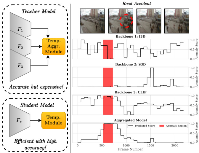
Figure 1. Left: A brief overview of our approach that distills the multi-backbone Teacher model’s knowledge to the Student model. In the Teacher model, representations from multiple backbones are aggregated using our proposed Temporal Aggregation Module. The single-backbone Student model is then trained with bi-level fine-grained knowledge distillation framework. Right: Framelevel predictions for individual backbones vs our proposed feature aggregation method on a video of a Road Accident from the testing set of UCF-Crime.
图 1: 左图: 我们方法的简要概述,将多主干教师模型的知识蒸馏到学生模型中。在教师模型中,通过我们提出的时序聚合模块 (Temporal Aggregation Module) 聚合来自多个主干网络的表征。随后使用双层细粒度知识蒸馏框架训练单主干学生模型。右图: 在UCF-Crime测试集的道路事故视频上,各主干网络的帧级预测与我们提出的特征聚合方法对比。
1. Introduction
1. 引言
Video Anomaly Detection (VAD) is a realization of automation based on video data which addresses the exhaustive labor and time requirements of video surveillance. The goal of a practical VAD system is to identify an activity that deviates from normal activities characterized by the training distribution [27].
视频异常检测 (VAD) 是基于视频数据实现自动化的一种方式,旨在解决视频监控中耗费大量人力和时间的问题。一个实用的 VAD 系统的目标是识别出与训练数据分布 [27] 所表征的正常活动存在偏差的行为。
Despite the extensive background of research in VAD [6, 13, 27, 29], the development of a robust model capable of accurately detecting anomalies within videos remains a difficult task. This challenge arises from the difficulty of modeling the s patio temporal characteristics of abnormal events, particularly those of rare occurrence and significant variability. This complexity is compounded by the laborintensive process of collecting frame-level annotations for video data, which presents a substantial barrier towards developing an effective VAD model for real-world scenarios. Prior works on VAD have adopted a practical approach by employing weakly-supervised learning which solely requires video-level labels to develop a model capable of making frame-level predictions [4, 6, 13, 14, 27, 29, 33, 34,
尽管在视频异常检测(VAD)领域已有大量研究背景 [6, 13, 27, 29],但开发能够准确检测视频中异常的鲁棒模型仍然是一项艰巨任务。这一挑战源于异常事件的时空特征建模困难,尤其是那些罕见发生且具有显著变异性的异常事件。由于视频数据需要人工密集的帧级标注工作,这种复杂性进一步加剧,这为开发适用于真实场景的有效VAD模型设置了重大障碍。先前关于VAD的研究采用了弱监督学习的实用方法,仅需视频级标签即可开发出能够进行帧级预测的模型 [4, 6, 13, 14, 27, 29, 33, 34,
37, 39, 41].
37, 39, 41].
Although weakly-supervised VAD is an intriguing approach, it suffers from limited supervision during training, resulting from the absence of precise frame-level annotations. To overcome this challenge, previous works [13, 27, 29] have employed knowledge transfer by combining a fixed backbone, pre-trained on general video represen- tation learning, with a dedicated prediction head to perform anomaly detection. Our exploratory evaluations, described in Figure 4, highlight that knowledge transfer has a substantial impact on the performance of weakly-supervised VAD. In particular, these evaluations suggest that the impact of the knowledge transfer is even more critical than the design choice of the prediction head: employing the knowledge of multiple pretrained backbones significantly enhances VAD performance. We attribute this performance boost to the complementary nature of knowledge from different backbones resulting from variations in inductive biases and pretraining datasets. In this work, we further analyze this observation by developing an aggregated model for weaklysupervised VAD.
虽然弱监督视频异常检测 (VAD) 是一种引人注目的方法,但由于缺乏精确的帧级标注,其训练过程中存在监督有限的问题。为克服这一挑战,先前的研究 [13, 27, 29] 采用了知识迁移策略,将经过通用视频表征学习预训练的固定主干网络与专用预测头相结合来进行异常检测。如图 4 所示,我们的探索性评估表明,知识迁移对弱监督 VAD 的性能具有显著影响。特别值得注意的是,这些评估表明知识迁移的影响甚至比预测头的设计选择更为关键:利用多个预训练主干网络的知识可以显著提升 VAD 性能。我们将这种性能提升归因于不同主干网络由于归纳偏差和预训练数据集的差异而产生的知识互补性。在本工作中,我们通过开发一个用于弱监督 VAD 的聚合模型来进一步分析这一现象。
A careful aggregation of the knowledge from multiple models is essential especially when the training supervision is weak, i.e., video-level supervision rather than frame-level supervision. To this aim, we propose a novel Temporal Aggregation Module (TAM) that combines s patio temporal information from the backbones through multiple self- and cross-attention mechanisms. This module comprehensively combines spatial (content) and temporal (positional) information from all the backbones to construct an effective aggregated representation of the video.
在训练监督较弱(即视频级监督而非帧级监督)的情况下,谨慎聚合多个模型的知识尤为重要。为此,我们提出了一种新颖的时间聚合模块(Temporal Aggregation Module,TAM),该模块通过多种自注意力和交叉注意力机制,从骨干网络中融合时空信息。该模块全面整合了所有骨干网络的空间(内容)和时间(位置)信息,以构建有效的视频聚合表示。
Our empirical evaluations, discussed later in Section 4, highlight the effectiveness of this aggregated model for weakly-supervised VAD. However, this model is computationally expensive for deployment due to incorporating multiple cumbersome backbones. To address this limitation, we develop a bi-level fine-grained knowledge distilla- tion mechanism, which distills the knowledge from the aggregated Teacher into an efficient Student, demonstrated in Figure 1. The distillation process enforces both predictionlevel and feature-level similarity between the Teacher and the Student. In the former, we align the output distributions of the Teacher and Student models to capture the detailed characteristics of the aggregated predictions. In the latter case, we align the representation-level knowledge to distill more complex, higher-order feature dependencies.
我们后续在第4节讨论的实证评估凸显了该聚合模型在弱监督视频异常检测(VAD)中的有效性。然而,由于融合了多个笨重的骨干网络,该模型在部署时计算成本高昂。为解决这一局限,我们开发了一种双层细粒度知识蒸馏机制,如图1所示,将聚合教师模型的知识蒸馏到高效学生模型中。该蒸馏过程同时强制教师模型与学生模型在预测层和特征层保持相似性:在预测层,我们对齐两个模型的输出分布以捕捉聚合预测的细节特征;在特征层,我们通过表征级知识对齐来蒸馏更复杂的高阶特征依赖关系。
Our results highlight that the proposed TAM and knowledge distillation approach are highly beneficial for weakly supervised VAD, where the learning signal is weak. In particular, we propose DAKD (Distilling Aggregated Knowledge with Disentangled Attention) that consists of a disentangled cross-attention-based Temporal Aggregation Module and a bi-level fine-grained knowledge distillation
我们的结果表明,所提出的TAM和知识蒸馏方法对于学习信号较弱的弱监督VAD非常有益。具体而言,我们提出了DAKD (Distilling Aggregated Knowledge with Disentangled Attention),它包含一个基于解耦交叉注意力的时序聚合模块和一个双层细粒度知识蒸馏
framework.
框架。
In summary, the contributions of our work are:
我们的工作贡献总结如下:
2. Related Work
2. 相关工作
Previous works on VAD can be categorized into two classes: Unsupervised VAD [2,7,8,16–20,23,30,31,35,36] and Weakly-supervised VAD [4, 6, 13, 14, 27, 29, 33, 34, 37, 39, 41]. Unsupervised VAD approaches such as Oneclass classification assume that merely normal videos are available for training and flag videos that have a considerable deviation from the learned distribution as anomalous [8, 19, 35]. However, the performance of these methods is limited and often results in a high false acceptance rate. This can be attributed to the fact that normal videos with novel events closely resemble abnormal events, and it is difficult to differentiate between the two events without the related context. Weakly-supervised VAD, on the other hand, leverages video-level labels and has gained popularity for its enhanced performance.
以往的视频异常检测(VAD)研究可分为两类: 无监督VAD [2,7,8,16–20,23,30,31,35,36]和弱监督VAD [4,6,13,14,27,29,33,34,37,39,41]。无监督方法如单类分类(Oneclass classification)假设训练时仅能获取正常视频, 并将显著偏离学习分布的视频标记为异常 [8,19,35]。但这类方法性能有限且误报率较高, 究其原因在于: 包含新事件的正视频与异常事件高度相似, 缺乏相关上下文时难以区分二者。相比之下, 弱监督VAD利用视频级标签获得了更优性能, 因而广受关注。
2.1. Weakly Supervised VAD
2.1. 弱监督视频异常检测 (Weakly Supervised VAD)
Sultani et al. [27] proposed a deep Multiple-Instance Learning (MIL) framework, incorporating sparsity and temporal smoothness constraints and knowledge transfer for enhancing anomaly localization. Zhong et al. [41] used a graph convolutional network to mitigate label noise, but had higher computational costs. Feng et al. [6] introduced a two-stage approach to fine-tune a backbone network for domain-specific knowledge. Tian et al. [29] used top $\mathbf{\nabla\cdot}\mathbf{k}$ instances and a multi-scale temporal network for feature magnitude learning. Li et al. [13] employed a scale-aware approach for capturing anomalous patterns using patch spatial relations. Zaheer et al. [37] minimized anomaly scores in normal regions with a Normalcy Suppression mechanism and introduced a clustering distance-based loss to improve discrimination. Despite current approaches, limited training data and weakly-supervised constraints restrict model learning. Knowledge transfer plays a crucial role in anomaly detection performance. Building upon the deep MIL framework [27], we propose architectural changes to enhance performance on unseen data.
Sultani等人[27]提出了一种深度多示例学习(Multiple-Instance Learning, MIL)框架,通过引入稀疏性、时间平滑约束和知识迁移来增强异常定位能力。Zhong等人[41]采用图卷积网络来减轻标签噪声,但计算成本较高。Feng等人[6]提出两阶段方法来微调骨干网络以获取领域特定知识。Tian等人[29]利用top $\mathbf{\nabla\cdot}\mathbf{k}$实例和多尺度时序网络进行特征量级学习。Li等人[13]采用尺度感知方法通过图像块空间关系捕捉异常模式。Zaheer等人[37]通过正常性抑制机制最小化正常区域的异常分数,并引入基于聚类距离的损失函数提升判别力。现有方法受限于训练数据不足和弱监督约束,影响了模型学习效果。知识迁移对异常检测性能具有关键作用。基于深度MIL框架[27],我们提出架构改进以提升模型在未见数据上的表现。
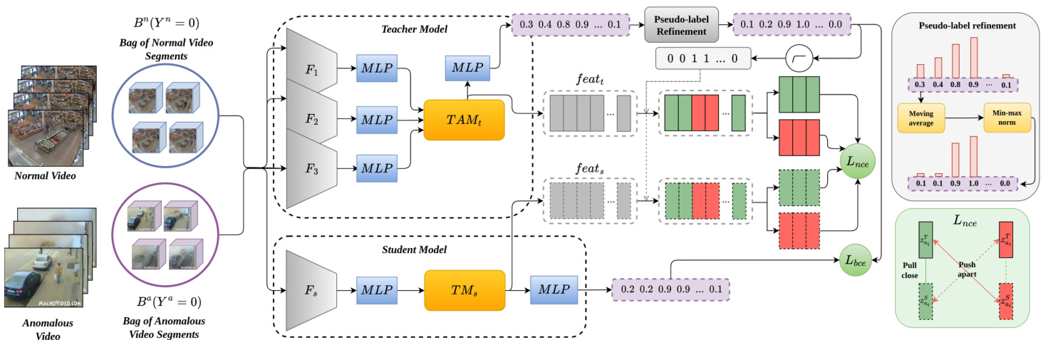
Figure 2. Schematic diagram of the proposed method. The Teacher model is initially trained with several feature extractors (Section 3.1) using the Temporal Aggregation Module (Section 3.2) in Stage 1. Stage 2: Feature-level and prediction-level knowledge distillation is performed to distill the knowledge of the complex Teacher model into the Student model (Section 3.3).
图 2: 所提方法示意图。阶段1中,教师模型(Teacher model)首先通过多个特征提取器(第3.1节)使用时态聚合模块(Temporal Aggregation Module)(第3.2节)进行训练。阶段2:通过特征级和预测级知识蒸馏,将复杂教师模型的知识提炼到学生模型(Student model)中(第3.3节)。
2.2. Knowledge Distillation
2.2. 知识蒸馏 (Knowledge Distillation)
Knowledge distillation is a technique to transfer knowledge from a complex Teacher model to a simpler Student model. Hinton et al. [11] introduced the concept of aligning Teacher and Student model probabilities. FitNets [26] extended distillation to intermediate-level hints, focusing on matching intermediate representations. Zagoruyko and Komodakis [12] introduced attention-based distillation to transfer attention maps. Papernot et al. [22] emphasized matching intermediate representations for effective knowledge transfer. Zhang et al. [40] introduced self-distillation, leveraging the Student model as a Teacher to improve genera liz ation. Heo et al. [10] improved knowledge transfer by distilling activation boundaries formed by hidden neurons.
知识蒸馏是一种将知识从复杂的教师模型 (Teacher) 转移到更简单的学生模型 (Student) 的技术。Hinton等人[11]提出了对齐教师模型和学生模型概率的概念。FitNets[26]将蒸馏扩展到中间层提示,专注于匹配中间表示。Zagoruyko和Komodakis[12]引入了基于注意力的蒸馏方法来传递注意力图。Papernot等人[22]强调匹配中间表示以实现有效的知识迁移。Zhang等人[40]提出了自蒸馏方法,利用学生模型作为教师模型来提升泛化能力。Heo等人[10]通过蒸馏隐藏神经元形成的激活边界改进了知识迁移效果。
3. Method
3. 方法
Weakly-supervised VAD aims to train models for framelevel anomaly detection using only video-level supervision. This approach faces challenges due to limited supervision and imbalanced training data, with anomalies typically occupying a small fraction of frames (e.g., $7.3%$ in UCFCrime dataset [27]). Previous works [13, 27, 29, 37, 41] address this by using knowledge transfer from large video datasets. We extend this approach by utilizing multiple backbones and introducing a novel fusion method for their representations. To mitigate the increased computational demands, we propose a distillation technique to compress the aggregated model’s knowledge into a single-backbone Student model. The following sections detail our feature extraction process (Section 3.1), temporal network for represent ation aggregation (Section 3.2), and the proposed distillation approach (Section 3.3).
弱监督视频异常检测 (VAD) 旨在仅使用视频级监督来训练帧级异常检测模型。由于监督有限且训练数据不平衡(异常帧通常只占很小比例,例如 UCFCrime 数据集 [27] 中仅占 $7.3%$),该方法面临挑战。先前工作 [13, 27, 29, 37, 41] 通过利用大型视频数据集的知识迁移来解决这一问题。我们通过使用多个主干网络并引入新颖的特征融合方法扩展了这一思路。为缓解计算需求增加的问题,我们提出一种蒸馏技术将聚合模型的知识压缩到单主干学生模型中。后续章节将详细阐述我们的特征提取流程(第 3.1 节)、用于特征聚合的时间网络(第 3.2 节)以及提出的蒸馏方法(第 3.3 节)。
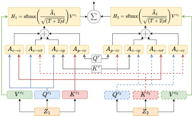
Figure 3. Schematic diagram of the proposed Temporal Aggregation Module. From the $Q^{c_{t}}$ , $K^{c_{t}}$ and $V^{c_{t}}$ vectors obtained from the representations of the $t^{t h}$ backbone and the relative positionbased vectors $Q^{r}$ and $K^{r}$ , four attention matrices are computed. $A_{c->c}$ is the self content-to-content attention, $A_{c->c^{\prime}}$ is the cross content-to-content attention, $A_{c->p}$ is the content-to-position attention and $A_{p->c}$ is the position-to-content attention. The output value is calculated in $H_{t}$ , and sftmx represents the softmax operation.
图 3: 提出的时序聚合模块示意图。从第 $t^{t h}$ 个主干表示获得的 $Q^{c_{t}}$、$K^{c_{t}}$ 和 $V^{c_{t}}$ 向量,以及基于相对位置的向量 $Q^{r}$ 和 $K^{r}$,计算得到四个注意力矩阵。$A_{c->c}$ 是自内容到内容的注意力,$A_{c->c^{\prime}}$ 是跨内容到内容的注意力,$A_{c->p}$ 是内容到位置的注意力,$A_{p->c}$ 是位置到内容的注意力。输出值在 $H_{t}$ 中计算,sftmx 表示 softmax 操作。
3.1. Feature Extraction
3.1. 特征提取
To alleviate the limited size of the training set and the highly imbalanced distribution of classes in weaklysupervised VAD, we adopt intensive knowledge transfer by employing multiple pre-trained video backbones for feature extraction. Different feature backbones encode different types of information, which can aid in anomaly detection and help circumvent the challenges arising from limited supervision. Additionally, different backbones can help increase the diversity of the extracted features, which can lead to a more comprehensive aggregated representation of the input videos.
为缓解弱监督视频异常检测(VAD)中训练集规模有限和类别分布高度不均衡的问题,我们采用密集知识迁移策略,通过多个预训练视频主干网络进行特征提取。不同特征主干网络能编码不同类型的信息,这既有助于异常检测,又能规避有限监督带来的挑战。此外,多样化的主干网络可提升特征多样性,从而生成更全面的视频聚合表征。
Consider that the video dataset consists of $n_{v}$ pairs ${(V_{i},y_{i})}{i=1}^{n_{v}}$ , where the $i^{t h}$ video, $V_{i}$ , is a sequence of clip instances $\mathbf{v}{i,j}$ and $y_{i}\in{0,1}$ is the corresponding video-level label. Let $\psi_{1},\ldots$ , $\psi_{T}$ denote the set of pretrained backbones for extracting representations from the input videos. For each input video clip $\mathbf{v}{i,j}$ , we extract fea- tures using the $t^{t h}$ backbone as $\mathbf{z}{i,j,t}=~\psi_{t}(\mathbf{v}{i,j})$ , where $\mathbf{z}{i,j,t}\in\mathbb{R}^{d_{t}}$ and $d_{t}$ denotes the cardinality of the output of the $t^{t h}$ backbone. After extracting representations using multiple backbones, we aggregate them using a novel Temporal Aggregation Module described in the next section.
假设视频数据集由 $n_{v}$ 对 ${(V_{i},y_{i})}{i=1}^{n_{v}}$ 组成,其中第 $i^{t h}$ 个视频 $V_{i}$ 是由片段实例 $\mathbf{v}{i,j}$ 组成的序列,而 $y_{i}\in{0,1}$ 是对应的视频级标签。设 $\psi_{1},\ldots$, $\psi_{T}$ 表示一组预训练骨干网络,用于从输入视频中提取表征。对于每个输入视频片段 $\mathbf{v}{i,j}$,我们使用第 $t^{t h}$ 个骨干网络提取特征 $\mathbf{z}{i,j,t}=~\psi_{t}(\mathbf{v}{i,j})$,其中 $\mathbf{z}{i,j,t}\in\mathbb{R}^{d_{t}}$,$d_{t}$ 表示第 $t^{t h}$ 个骨干网络输出的维度。在使用多个骨干网络提取表征后,我们通过下一节描述的新型时序聚合模块 (Temporal Aggregation Module) 对它们进行聚合。
3.2. Temporal Aggregation Module
3.2. 时序聚合模块
In weakly-supervised VAD, incorporating relative positional information is vital due to the low-pass temporal frequency characteristics of natural events, where anomalous frames cluster together rather than appearing sporadically. Leveraging this information enhances anomaly detection performance, which we achieve by utilizing a disentangled attention mechanism that inherently accounts for relative positional information during attention computation. This mechanism [9] employs a relative positional bias, with the maximum relative distance parameterized by $k$ . The relative distance between positions $i$ and $j$ is encoded by the function $\gamma(i,j)$ , constrained within $[0,2k)$ , thereby reducing attention model complexity and making it suitable for low-data and weak-supervision scenarios. Formally,
在弱监督视频异常检测(VAD)中,由于自然事件具有低频时间特性(异常帧往往聚集出现而非零星分布),整合相对位置信息至关重要。我们通过采用解耦注意力机制(该机制在注意力计算中天然包含相对位置信息)来提升异常检测性能。该机制[9]采用相对位置偏置,最大相对距离由参数$k$决定。位置$i$与$j$之间的相对距离通过函数$\gamma(i,j)$编码,其值域约束在$[0,2k)$范围内,从而降低注意力模型复杂度,使其适用于低数据和弱监督场景。
The disentangled attention has three attention components: i) content-to-content attention: This component attends to the content of a token at position $i$ by interacting with the content of the token at position $j$ within the same sequence, ii) content-to-position attention: This attention component considers the content of token $i$ and its relative position to token $j$ , capturing how the content of token $i$ influences its attention weight concerning token $j$ . iii) position-to-content attention: Similarly, this component assesses the content of token $j$ and its relative position to token $i.$ , elucidating how the content at position $j$ influences its attention weight with respect to token $i$ .
解耦注意力 (disentangled attention) 包含三个注意力组件:
i) 内容到内容注意力 (content-to-content attention):该组件通过同一序列中位置 $i$ 的 token 内容与位置 $j$ 的 token 内容交互,关注位置 $i$ 的 token 内容;
ii) 内容到位置注意力 (content-to-position attention):该组件考虑 token $i$ 的内容及其与 token $j$ 的相对位置,捕捉 token $i$ 的内容如何影响其对 token $j$ 的注意力权重;
iii) 位置到内容注意力 (position-to-content attention):类似地,该组件评估 token $j$ 的内容及其与 token $i$ 的相对位置,阐明位置 $j$ 的内容如何影响其对 token $i$ 的注意力权重。
We further disentangle this attention mechanism to adopt it for multi-input scenarios. To this aim, we add a crossattention module to fuse information from multiple input sequences. Table 5 evaluates the contribution of each of these attention components. Given $T$ input sequences $Z_{t}$ , $t~\in~{1,\ldots,T}$ , we define the query, key, and value for each of the representations as:
我们进一步解耦这一注意力机制,使其适用于多输入场景。为此,我们添加了一个交叉注意力模块来融合多个输入序列的信息。表5评估了这些注意力组件的各自贡献。给定$T$个输入序列$Z_{t}$,$t~\in~{1,\ldots,T}$,我们将每个表征的查询、键和值定义为:
$$
Q^{c_{t}}=Z_{t}W_{q,c_{t}},\quad K^{c_{t}}=Z_{t}W_{k,c_{t}},\quad V^{c_{t}}=Z_{t}W_{v,c_{t}}.
$$
$$
Q^{c_{t}}=Z_{t}W_{q,c_{t}},\quad K^{c_{t}}=Z_{t}W_{k,c_{t}},\quad V^{c_{t}}=Z_{t}W_{v,c_{t}}.
$$
The shared relative position key and query are also computed as :
共享的相对位置键和查询也计算为:
$$
Q^{r}=\tilde{Z}W_{q,r},\quad K^{r}=\tilde{Z}W_{k,r},
$$
$$
Q^{r}=\tilde{Z}W_{q,r},\quad K^{r}=\tilde{Z}W_{k,r},
$$
where Z E R2kxd represents the relative position embedding vectors shared across all layers and backbones (i.e., staying fixed during forward propagation).
其中 Z E R2kxd 表示所有层和骨干网络共享的相对位置嵌入向量 (即在正向传播过程中保持固定)。
Our aggregation attention mechanism is then formulated as:
我们的聚合注意力机制公式如下:
$$
\begin{array}{r l}{\lefteqn{\tilde{A}{i,j,t}=\underbrace{Q_{i}^{c_{t}}K_{j}^{c_{t}\top}}{\mathrm{(self content-to-content)}}+\underbrace{\sum_{h,h\neq t}Q_{i}^{c_{t}}K_{j}^{c_{h}\top}}{\mathrm{(cross~content-to-content)}}}}\ {+\underbrace{Q_{i}^{c_{t}}K_{\gamma(i,j)}^{r}}{\mathrm{(content-to-position)}}+\underbrace{K_{j}^{c_{t}}Q_{\gamma(j,i)}^{r}}_{\mathrm{(position-to-content)}},}\end{array}
$$
and the output is computed as:
输出计算为:
$$
H_{t}=s o f t m a x\big(\frac{\tilde{A}{t}}{\sqrt{(T+2)d}}\big)V^{c_{t}},
$$
$$
H_{t}=s o f t m a x\big(\frac{\tilde{A}{t}}{\sqrt{(T+2)d}}\big)V^{c_{t}},
$$
where $T$ is the number of backbones, and the final aggregated output is $\begin{array}{r}{H=\frac{1}{T}\sum_{t}H_{t}}\end{array}$ . $Q^{c_{t}}$ , $K^{c_{t}}$ , and $V^{c_{t}}$ are content vectors derived thrPough projection matrices $W_{q,c_{t}}$ , $W_{k,c_{t}},W_{v,c_{t}}\in\mathbb{R}^{d\times d}$ and $t\in{1,\ldots,T}$ is the index of the backbone. $Q_{r}$ and $K_{r}$ correspond to the projected relative position vectors, facilitated by projection matrices $W_{q,r}$ and $\bar{W}_{k,r}\in\mathbb{R}^{d\times d}$ , respectively. The architecture of the Temporal Aggregation Module integrates the aforementioned disentangled attention mechanism to improve the relative encoding and fusing of representations from multiple backbones.
其中 $T$ 是骨干网络数量,最终聚合输出为 $\begin{array}{r}{H=\frac{1}{T}\sum_{t}H_{t}}\end{array}$。$Q^{c_{t}}$、$K^{c_{t}}$ 和 $V^{c_{t}}$ 是通过投影矩阵 $W_{q,c_{t}}$、$W_{k,c_{t}},W_{v,c_{t}}\in\mathbb{R}^{d\times d}$ 得到的内容向量,$t\in{1,\ldots,T}$ 表示骨干网络索引。$Q_{r}$ 和 $K_{r}$ 对应由投影矩阵 $W_{q,r}$ 和 $\bar{W}_{k,r}\in\mathbb{R}^{d\times d}$ 映射的相对位置向量。时序聚合模块 (Temporal Aggregation Module) 的架构整合了上述解耦注意力机制,以改进多骨干网络表征的相对编码与融合。
3.3. Bi-level Fine-grained Knowledge Distillation
3.3. 双层细粒度知识蒸馏
Our approach leverages the knowledge from multiple pre-trained backbones, allowing it to benefit from their collective expertise. We employ the MIL ranking approach, proposed by Sultani et al. [27] for training the first stage aggregated model. This intensive knowledge transfer aims to address the scarcity of supervision, which often hinders learning in the current weakly-supervised learning setup. However, using multiple backbones drastically increases computational overhead, thereby making the model less suitable for real-world applications. To overcome these issues, we develop a knowledge distillation approach, as shown in Figure 2, that distills the knowledge of the aggregated Teacher at prediction and representation levels
我们的方法利用多个预训练主干网络的知识,使其能够受益于它们的集体专长。我们采用Sultani等人[27]提出的MIL排序方法训练第一阶段聚合模型。这种密集的知识迁移旨在解决监督稀缺问题,该问题常阻碍当前弱监督学习设置下的模型训练。然而,使用多个主干网络会显著增加计算开销,从而使模型难以适用于实际应用。为解决这些问题,我们开发了一种知识蒸馏方法(如图2所示),该方法在预测和表征层面蒸馏聚合教师模型的知识
into the Student model.
将知识融入学生模型。
Prediction-level distillation: In the first level of distillation, we align the output distributions of the Teacher and Student models using the cross-entropy loss function [11]. Weakly-supervised VAD methods [13, 27, 29] generally use a single segment or top $\mathbf{\nabla\cdot}\mathbf{k}$ segments for the given input during the training since they solely have access to the videolevel annotation. However, for distillation, despite the lack of fine-grained ground truth labels, we use the Teacher’s segment-level predictions to provide robust learning signals. These predictions act as soft pseudo-labels for training the Student model. The trained aggregated model generates scores for anomalous videos marked as $\ensuremath{\boldsymbol{S}}^{a}={\ensuremath{\boldsymbol{s}}{i}^{a}}{i=1}^{n_{s}}$ where $n_{s}$ is the number of segments. Based upon [6], to remove the jitter and refine the anomaly scores, we use a convolutional kernel of size $\epsilon$ as a moving average filter and use min-max normalization afterward. Min-max normalization helps to focus on the anomalous segments during training. The impact of using moving average filter and min-max normalization is presented in Table 4. Min-max normalization and moving average filter are described as:
预测级蒸馏:在第一级蒸馏中,我们使用交叉熵损失函数[11]对齐教师模型和学生模型的输出分布。弱监督视频异常检测方法[13,27,29]通常仅使用单个片段或前$\mathbf{\nabla\cdot}\mathbf{k}$个片段进行训练,因为它们只能获取视频级标注。但在蒸馏过程中,尽管缺乏细粒度真实标签,我们利用教师模型的片段级预测来提供稳健的学习信号。这些预测作为软伪标签用于训练学生模型。训练后的聚合模型为异常视频生成分数,记为$\ensuremath{\boldsymbol{S}}^{a}={\ensuremath{\boldsymbol{s}}{i}^{a}}{i=1}^{n_{s}}$,其中$n_{s}$表示片段数量。基于[6]的研究,为消除抖动并优化异常分数,我们采用尺寸为$\epsilon$的卷积核作为移动平均滤波器,随后进行最小-最大归一化处理。最小-最大归一化有助于训练过程中聚焦异常片段。移动平均滤波器和最小-最大归一化的效果对比见表4。最小-最大归一化与移动平均滤波器的计算公式如下:
$$
\begin{array}{l l}{\displaystyle\hat{y}{i}^{a}=\frac{\tilde{s}{i}^{a}-\operatorname*{min}(\tilde{S}^{a})}{\operatorname*{max}(\tilde{S}^{a})-\operatorname*{min}(\tilde{S}^{a})},}&{i\in[1,n_{s}],}\ {\displaystyle\tilde{s}{i}^{a}=\frac{1}{2\epsilon}\sum_{j=i-\epsilon}^{i+\epsilon}s_{j}^{a},}&\end{array}
$$
$$
\begin{array}{l l}{\displaystyle\hat{y}{i}^{a}=\frac{\tilde{s}{i}^{a}-\operatorname*{min}(\tilde{S}^{a})}{\operatorname*{max}(\tilde{S}^{a})-\operatorname*{min}(\tilde{S}^{a})},}&{i\in[1,n_{s}],}\ {\displaystyle\tilde{s}{i}^{a}=\frac{1}{2\epsilon}\sum_{j=i-\epsilon}^{i+\epsilon}s_{j}^{a},}&\end{array}
$$
respectively, where min and max functions compute the minimum and maximum scores in the given set.
分别表示给定集合中的最小和最大分数,其中min和max函数分别计算最小和最高分。
We refine the anomaly scores into $Y^{a}={\hat{y}{i}^{a}}{i=1}^{n_{s}}$ and use these as soft pseudo-labels. Since we are certain about the segment-level annotation in the normal videos, we can combine the soft anomaly labels with normal videos. Given the nature of the VAD task, which typically involves predictions for two classes, the conventional posterior matching approach encounters limitations due to the limited support of the distribution. To mitigate this issue, we extend the distillation process to operate at the feature level, employing the InfoNCE loss [21, 28].
我们将异常分数精炼为 $Y^{a}={\hat{y}{i}^{a}}{i=1}^{n_{s}}$ ,并将其用作软伪标签。由于我们对正常视频中的片段级标注有把握,因此可以将软异常标签与正常视频结合。鉴于视频异常检测 (VAD) 任务通常涉及两类预测的特性,传统后验匹配方法会因分布支持有限而遇到局限性。为缓解这一问题,我们扩展了蒸馏过程,使其在特征层面运作,并采用 InfoNCE 损失 [21, 28]。
Feature-level distillation: In the context of feature-level distillation, we utilize a multilayer perceptron (MLP) with a single hidden layer to transform the input representations $\mathbf{h}{i}$ from both the Student and Teacher models into corresponding feature vectors $ {\bf z}{i}=g({\bf h}{i})=W^{(2)}\sigma(W^{(1)}{\bf h}{i})$ , with $\sigma$ representing the ReLU non linearity [1]. Subsequently, leveraging the Teacher model’s prediction outputs, we determine class labels for individual features by applying a threshold $\delta$ . This facilitates the identification of four distinct feature subsets: ${\mathbf z}{a}^{T}$ (anomaly features of the Teacher), ${\bf z}{n}^{T}$ (normal features of the Teacher), ${\mathbf z}{a}^{S}$ (anomaly features for the Student), and $\mathbf{z}_{n}^{S}$ (normal features of the Student). Here, the superscripts $T$ and $S$ denote the Teacher and Student models, respectively. We utilize cosine similarity, denoted as $\mathrm{sim}(.,.)$ , as a measure of similarity between input vectors.
特征级蒸馏:在特征级蒸馏的背景下,我们采用单隐藏层的多层感知机 (MLP) 将学生模型和教师模型的输入表征 $\mathbf{h}{i}$ 转换为对应的特征向量 ${\bf z}{i}=g({\bf h}{i})=W^{(2)}\sigma(W^{(1)}{\bf h}{i})$,其中 $\sigma$ 表示 ReLU 非线性激活函数 [1]。随后,基于教师模型的预测输出,通过设定阈值 $\delta$ 为单个特征确定类别标签。这有助于识别四个不同的特征子集:${\mathbf z}{a}^{T}$(教师异常特征)、${\bf z}{n}^{T}$(教师正常特征)、${\mathbf z}{a}^{S}$(学生异常特征)和 $\mathbf{z}_{n}^{S}$(学生正常特征)。此处上标 $T$ 和 $S$ 分别表示教师模型和学生模型。我们使用余弦相似度 $\mathrm{sim}(.,.)$ 作为输入向量间的相似性度量。
Our feature distillation loss using InfoNCE is defined as:
我们采用InfoNCE的特征蒸馏损失定义为:
$$
\begin{array}{r l r}{}{\mathcal{L}{n c e}=-\log\frac{e^{\mathrm{sim}(\mathbf{z}{a_{i}}^{T},\mathbf{z}{a_{i}}^{S})/\tau}}{\sum_{k=1}^{N}e^{\mathrm{sim}(\mathbf{z}{a_{i}}^{T},\mathbf{z}{n_{k}}^{S})/\tau}+e^{\mathrm{sim}(\mathbf{z}{a_{i}}^{T},\mathbf{z}{a_{i}}^{S})/\tau}}}\ {}{-\log\frac{e^{\mathrm{sim}(\mathbf{z}{n_{i}}^{T},\mathbf{z}{n_{i}}^{S})/\tau}}{\sum_{k=1}^{N}e^{\mathrm{sim}(\mathbf{z}{n_{i}}^{T},\mathbf{z}{a_{k}}^{S})/\tau}+e^{\mathrm{sim}(\mathbf{z}{n_{i}}^{T},\mathbf{z}{n_{i}}^{S})/\tau}},}\end{array}
$$
where $\tau$ represents the temperature parameter. The complete loss function for the distillation is as follows:
其中 $\tau$ 表示温度参数。蒸馏的完整损失函数如下:
$$
\mathcal{L}{d}=\mathcal{L}{b c e}(y^{T},y^{S})+\alpha\tau^{2}\mathcal{L}_{n c e}(T,S),
$$
$$
\mathcal{L}{d}=\mathcal{L}{b c e}(y^{T},y^{S})+\alpha\tau^{2}\mathcal{L}_{n c e}(T,S),
$$
where $\mathcal{L}{n c e}$ represents the feature-level distillation loss using InfoNCE, $\mathcal{L}{b c e}$ represents the BCE loss, $\mathcal{L}_{d}$ represents the combined loss for distillation, and $\alpha$ represents the scaling coefficient to control the contribution of the two loss terms.
其中 $\mathcal{L}{n c e}$ 表示使用 InfoNCE 的特征级蒸馏损失,$\mathcal{L}{b c e}$ 表示 BCE 损失,$\mathcal{L}_{d}$ 表示蒸馏的组合损失,$\alpha$ 表示控制两个损失项贡献的缩放系数。
4. Experiments
4. 实验
4.1. Datasets and Metrics
4.1. 数据集与评估指标
Our model is evaluated on three benchmark datasets for weakly-supervised VAD: UCF-Crime, Shanghai Tech, and XD-Violence. The UCF-Crime dataset [27] contains 1900 untrimmed videos totaling 128 hours, captured by surveillance cameras in diverse real-world settings, with 13 types of anomalies. The Shanghai Tech dataset [16] comprises 437 videos from fixed-angle street cameras, featuring 13 background scenes. We follow Zhong et al.’s [41] approach to adapt it for weakly-supervised learning. The XD-Violence dataset [34] is a comprehensive multiscene collection sourced from various media, containing 4754 untrimmed videos spanning over 217 hours. All three datasets provide video-level labels for training and framelevel labels for testing, allowing for robust evaluation of weakly-supervised VAD models across diverse scenarios and anomaly types.
我们的模型在三个弱监督视频异常检测(VAD)基准数据集上进行了评估:UCF-Crime、Shanghai Tech和XD-Violence。UCF-Crime数据集[27]包含1900段未剪辑视频,总计128小时,由不同真实场景下的监控摄像头拍摄,包含13类异常行为。Shanghai Tech数据集[16]包含437段固定角度街道摄像头拍摄的视频,涵盖13种背景场景。我们采用Zhong等人[41]的方法将其适配于弱监督学习。XD-Violence数据集[34]是一个多场景综合数据集,采集自各类媒体资源,包含4754段未剪辑视频,总时长超过217小时。这三个数据集均提供视频级标签用于训练和帧级标签用于测试,能够全面评估弱监督VAD模型在不同场景和异常类型下的性能。
Evaluation Metrics: In order to assess the effectiveness of our approach, we utilize the frame-based receiver operating characteristic (ROC) curve and the area under the curve (AUC), which have been commonly used in previous studies on anomaly detection [6, 27, 29]. Based on [34], we use average precision (AP) as the evaluation measure for the XD-Violence dataset.
评估指标:为了评估我们方法的有效性,我们采用了基于帧的接收者操作特征曲线 (ROC) 和曲线下面积 (AUC) ,这些指标在以往异常检测研究中被广泛使用 [6, 27, 29]。根据 [34] 的研究,我们使用平均精度 (AP) 作为 XD-Violence 数据集的评估指标。
4.2. Implementation Details
4.2. 实现细节
Our proposed method is implemented using PyTorch [24]. We divide each video into 32 non-overlapping
我们提出的方法使用PyTorch [24]实现。我们将每个视频划分为32个不重叠的
Table 1. Comparison of the proposed Temporal Aggregation Module (TAM) with other variants including the MTN module from RTFM. We observe that TAM is superior to other temporal models at capturing spatio-temporal dependencies.
表 1: 提出的时序聚合模块 (Temporal Aggregation Module, TAM) 与其他变体 (包括 RTFM 中的 MTN 模块) 的对比。我们观察到 TAM 在捕捉时空依赖性方面优于其他时序模型。
| TemporalNetwork | AUC(%) |
|---|---|
| MTN | 85.31 |
| MultiheadAttention | 86.28 |
| LSTM | 86.97 |
| RNN | 86.99 |
| Disentangled Attention | 87.09 |
| GRU | 87.53 |
| 1DCNN | 87.72 |
| TAM | 88.34 |
| 方法 | 特征 | T=32 | AUC (%) |
|---|---|---|---|
| Sultani et al. [27] | C3D-RGB | 75.41 | |
| Sultani et al. [27] | I3D-RGB | 77.92 | |
| Zhang et al. [39] | C3D-RGB | 78.66 | |
| GCN [41] | TSN-RGB | 82.12 | |
| MIST [6] | I3D-RGB | - | 82.30 |
| Wu et al. [34] | I3D-RGB | 82.44 | |
| CLAWS [37] | C3D-RGB | - | 83.03 |
| RTFM* [29] | I3D-RGB | √ | 84.30 |
| Wu et al. [33] | I3D-RGB | 84.89 | |
| MSL [14] | I3D-RGB | √ | 85.30 |
| MSL [14] | VSwin-RGB | 85.62 | |
| S3R [32] | I3D-RGB | 85.99 | |
| SSRL* [13] | I3D-RGB | 人 | 86.79 |
| MGFN [4] | I3D-RGB | 人 | 86.98 |
| DAKDT (Ours) | Multiple | 88.15 | |
| DAKDs (Ours) | I3D | 人 | 88.10 |
| DAKDs (Ours) | CLIP | 88.34 |
Table 2. Comparison with existing weakly-supervised methods on UCF-Crime dataset. $\mathrm{DAKD}{T}$ and $\mathrm{DAKD}_{S}$ denote Teacher and Student models. $\mathrm{T}\mathrm{=}32$ indicates 32 non-overlapping video segments. Features column shows backbone used for feature extraction. Asterisk $({}^{*})$ indicates methods for which we could not validate the performance using the official code or our implementation. Results are the average over five independent runs.
表 2: 在UCF-Crime数据集上与现有弱监督方法的对比。$\mathrm{DAKD}{T}$和$\mathrm{DAKD}_{S}$分别表示教师模型和学生模型。$\mathrm{T}\mathrm{=}32$表示32个不重叠的视频片段。"Features"列显示用于特征提取的主干网络。星号$({}^{*})$表示我们无法通过官方代码或自行实现验证性能的方法。结果为五次独立运行的平均值。
segments to pass through the feature extractors.
片段通过特征提取器。
Teacher Model: For the Teacher Model, we utilize the I3D [3], S3D [38], and CLIP [25] backbones to obtain representations for the video inputs. Before aggregation, the feature vectors are projected to a common dimension (512) using two-layer MLPs with ReLU [1] activation in the first layer. The input dimension for the MLPs processing I3D and S3D features is 1024, while for the one processing CLIP representations is 512. The hidden dimension is 512 for each of the three MLPs.
教师模型 (Teacher Model):对于教师模型,我们采用 I3D [3]、S3D [38] 和 CLIP [25] 作为主干网络来获取视频输入的表示。在聚合之前,特征向量通过带有 ReLU [1] 激活函数的两层 MLP (多层感知机) 投影到一个共同的维度 (512)。处理 I3D 和 S3D 特征的 MLP 输入维度为 1024,而处理 CLIP 表示的 MLP 输入维度为 512。三个 MLP 的隐藏层维度均为 512。
In our Temporal Aggregation Module, we utilize disentangled attention along with our proposed cross-attention mechanism to combine multiple inputs, as explained in
在我们的时序聚合模块中,我们利用解耦注意力机制 (disentangled attention) 和提出的交叉注意力机制 (cross-attention mechanism) 来融合多个输入,具体说明如下:
Section 3.2. The disentangled attention module has one hidden layer with a hidden embedding dimension of 1024 and 8 attention heads. Notably, the TAM shares positional embeddings among all backbones. We experimented with values of maximum relative distance $k$ from 1 to 32, where 32 is the maximum segment index, to determine the optimal value that constrains the maximum distance between two positions $(i,j)$ in disentangled attention. The aggregated features are then passed through a feed forward network with hidden dimensions of 512 and 32, and with a sigmoid activation in the final layer to obtain the segment-level prediction. The conventional MIL Loss [27] serves as the loss function during training.
第3.2节 解耦注意力模块包含一个隐藏层,其隐藏嵌入维度为1024并配备8个注意力头。值得注意的是,TAM在所有骨干网络间共享位置嵌入。我们通过实验测试了最大相对距离$k$从1到32(其中32为最大片段索引)的不同取值,以确定能约束解耦注意力中两个位置$(i,j)$间最大距离的最优值。聚合后的特征随后通过前馈网络处理,该网络隐藏维度分别为512和32,并在最终层采用sigmoid激活函数来获得片段级预测。训练过程中采用传统MIL损失函数[27]。
Student Model: In the Student Model, we use the CLIP [25] backbone which has shown notable performance in video analysis tasks [15]. We then pass the representations to the Temporal Module. The Temporal Module uses the disentangled attention mechanism with the omission of cross content-to-content attention term. The attention normalization factor is also adjusted based on the single backbone formulation. The dimensionality of embeddings and the number of attention heads is similar to Teacher model formulation. We train the Student model with the bi-level fine-grained knowledge distillation approach as discussed in Section 3.3. Employing contrastive loss for representation-level distillation, we mask the positive and negative examples using the threshold $\delta=0.9$ on the Teacher’s predictions. Then we calculate the cosine similarity between the samples from the Teacher and Student and obtain the loss for cross-positive and cross-negative examples. For prediction-level distillation, we use the BCE loss function to align the output distributions. Finally, we use a linear combination of the two loss terms using the parameter $\alpha$ to calculate the final loss. We also scale the $\mathcal{L}_{n c e}$ loss by $\tau^{2}$ (Equation 8) which results in better training.
学生模型 (Student Model):在学生模型中,我们采用CLIP[25]主干网络,该架构在视频分析任务中表现出卓越性能[15]。随后将表征输入时序模块 (Temporal Module),该模块采用解耦注意力机制 (disentangled attention mechanism),并省略了内容间交叉注意力项 (cross content-to-content attention term)。注意力归一化因子也根据单主干架构进行调整,其嵌入维度和注意力头数量与教师模型 (Teacher model) 配置保持一致。如第3.3节所述,我们采用双层细粒度知识蒸馏方法训练学生模型:在表征级蒸馏中使用对比损失 (contrastive loss),通过教师模型预测值阈值 ($\delta=0.9$) 屏蔽正负样本,计算师生样本间的余弦相似度以获得跨正/负样本损失;在预测级蒸馏中采用BCE损失函数对齐输出分布。最终通过参数 $\alpha$ 线性组合两项损失,并按 $\tau^{2}$ (公式8) 缩放 $\mathcal{L}_{n c e}$ 损失以优化训练效果。
The Teacher and Student models are trained for 100 epochs, using the Adagrad optimizer [5] with a weight decay of 0.001 and a learning rate of 0.0001 for the temporal models and 0.001 otherwise. The training batch size is 60, and each batch consists of 30 normal and 30 anomalous video clips.
教师模型和学生模型训练了100个周期,使用Adagrad优化器[5],时间模型的权重衰减为0.001、学习率为0.0001,其他情况下学习率为0.001。训练批次大小为60,每个批次包含30个正常视频片段和30个异常视频片段。
4.3. Comparison with the state of the art
4.3. 与当前最优技术的对比
Table 2 presents our main results on the UCF-Crime dataset, while Table 3 shows the results for the ShanghaiTech and XD-Violence datasets. $\mathrm{DAKD}{T}$ and $\mathrm{DAKD}{S}$ outperform all the existing weakly-supervised methods by a significant margin on all the datasets. Remarkably, on the UCF-Crime dataset, $\mathrm{DAKD}{S}$ outperforms current SOTA methods, MGFN [4] by $1.36%$ , SSRL [13] by $1.55%$ , S3R [32] by $2.35%$ , and RTFM [29] by $4.04%$ . $\mathrm{DAKD}_{S}$ is also extremely efficient compared to SSRL, which uses multiscale video crops for training, making it suitable for realworld use. Additionally, DAKD also achieves an AUC score of $98.10%$ on the Shanghai Tech dataset, providing superior performance although the performance of previous methods seems to be saturated on this dataset. Moreover, DAKD achieves an AP score of $85.61%$ on the XDViolence dataset and outperforms existing methods by a significant margin.
表 2 展示了我们在 UCF-Crime 数据集上的主要结果,而表 3 则显示了 ShanghaiTech 和 XD-Violence 数据集的结果。$\mathrm{DAKD}{T}$ 和 $\mathrm{DAKD}{S}$ 在所有数据集上均显著优于现有的弱监督方法。值得注意的是,在 UCF-Crime 数据集上,$\mathrm{DAKD}{S}$ 以 $1.36%$ 的优势超越当前 SOTA 方法 MGFN [4],以 $1.55%$ 超越 SSRL [13],以 $2.35%$ 超越 S3R [32],并以 $4.04%$ 超越 RTFM [29]。与使用多尺度视频裁剪训练的 SSRL 相比,$\mathrm{DAKD}_{S}$ 也极为高效,适合实际应用。此外,DAKD 在 ShanghaiTech 数据集上取得了 $98.10%$ 的 AUC 分数,尽管先前方法在该数据集上的性能似乎已趋于饱和,但仍提供了卓越的性能。此外,DAKD 在 XD-Violence 数据集上实现了 $85.61%$ 的 AP 分数,并显著优于现有方法。

Figure 4. Ablation study on the UCF-Crime dataset to investigate the impact of feature backbones used in the Teacher Model. We observe that the involvement of the CLIP backbone significantly boosts the AUC score. The combination of jointly using all three backbones (I3D, S3D, and CLIP) provides the best performance.
图 4: 在UCF-Crime数据集上进行的消融研究,用于探究教师模型(Teacher Model)中不同特征主干网络的影响。我们发现CLIP主干网络的加入显著提升了AUC分数。同时使用所有三种主干网络(I3D、S3D和CLIP)的组合取得了最佳性能。
We further analyze the performance of the models on each anomaly class in UCF-Crime to highlight the effectiveness of DAKD. Figure 6 presents the class-wise AUC scores for the Anomaly classes in UCF-Crime of our method compared with that of Sultani et al. [27] and RTFM [29]. Our approach outperforms existing methods by a significant margin in classes such as Assault, Arrest, Burglary, Explosion, and Vandalism.
我们进一步分析模型在UCF-Crime各异常类别上的性能,以凸显DAKD的有效性。图6展示了我们的方法在UCF-Crime异常类别上的分类AUC分数,并与Sultani等人[27]和RTFM[29]的方法进行对比。在Assault、Arrest、Burglary、Explosion和Vandalism等类别上,我们的方法显著优于现有方法。
4.4. Ablation Study
4.4. 消融实验
Analysis of Different Feature Backbones: Ablation studies were conducted to assess the impact of different pre-trained feature backbones on our Teacher Model’s training. Specifically, we utilized three feature backbones: I3D [3], S3D [38], and CLIP [25]. The results of these ablation studies can be found in Figure 4. It is evident from the figure that configurations involving the CLIP backbone consistently outperform other combinations. Notably, the combination involving all three backbones yields the best performance and is consequently adopted for training the Teacher Model. This choice not only enhances the diversity of input features but also mitigates the challenges posed by the limited availability of training data.
不同特征主干网络的分析:我们进行了消融实验以评估不同预训练特征主干网络对教师模型训练的影响。具体而言,我们使用了三种特征主干网络:I3D [3]、S3D [38] 和 CLIP [25]。这些消融实验的结果如图 4 所示。从图中可以明显看出,采用 CLIP 主干网络的配置始终优于其他组合。值得注意的是,同时使用三种主干网络的组合能获得最佳性能,因此被采用来训练教师模型。这一选择不仅增强了输入特征的多样性,还缓解了训练数据有限带来的挑战。
Analysis of Different Temporal Modules: We study the impact of the proposed Temporal Aggregation Module compared to prominent temporal networks. The feature representations obtained from the I3D [3], S3D [38], and
不同时序模块分析:我们研究了提出的时序聚合模块(Temporal Aggregation Module)与主流时序网络(I3D [3]、S3D [38])所获特征表示的效果对比。
Table 3. Performance comparison with existing weaklysupervised methods on Shanghai Tech (SHT, AUC score) and XDViolence (XDV, AP score) datasets. $\mathrm{DAKD}{T}$ and $\mathrm{DAKD}_{S}$ denote Teacher and Student models. Other notations as in Table 2.
表 3. 现有弱监督方法在 Shanghai Tech (SHT, AUC 分数) 和 XDViolence (XDV, AP 分数) 数据集上的性能对比。$\mathrm{DAKD}{T}$ 和 $\mathrm{DAKD}_{S}$ 分别表示教师模型和学生模型。其他符号含义与表 2 相同。
| 方法 | 特征 | T=32 | SHT | XDV |
|---|---|---|---|---|
| Sultani et al.[27] | C3D-RGB | 86.30 | 73.20 | |
| Zhangetal.[39] | C3D-RGB | 82.50 | ||
| MIST [6] | I3D-RGB | 94.83 | ||
| CLAWS [37] | C3D-RGB | - | 89.67 | |
| RTFM* [29] | I3D-RGB | 97.21 | 77.81 | |
| Wu et al.[34] | I3D-RGB | √ | 78.64 | |
| Wu et al.[33] | I3D-RGB | 97.48 | ||
| MSL [14] | I3D-RGB | 96.08 | 78.28 | |
| SSRL* [13] | I3D-RGB | 97.04 | - | |
| MSL [14] | VSwin-RGB | 97.32 | 78.59 | |
| DAKDr (Ours) | Multiple | 98.08 | 84.78 | |
| DAKDs (Ours) | I3D | 98.02 | 85.12 | |
| DAKDs (Ours) | CLIP | 98.10 | 85.61 |
CLIP [25] backbones are passed to the specified temporal module. The particular results are presented in Table 1. From Table 1, we can see that the proposed TAM specification outperforms other popular temporal networks in terms of the AUC score. Notably, TAM outperforms vanilla disentangled attention and multihead attention mechanisms showing its efficacy.
CLIP [25] 主干网络被传递到指定的时序模块。具体结果如表 1 所示。从表 1 中可以看出,所提出的 TAM 规范在 AUC 分数方面优于其他流行的时序网络。值得注意的是,TAM 优于普通的解耦注意力 (vanilla disentangled attention) 和多头注意力 (multihead attention) 机制,展现了其有效性。
Analysis of Other Parameters: We investigated the effects of several key training parameters, as shown in Figure 5 and Table 4. Increasing the temperature $\tau$ in the $\mathcal{L}{n c e}$ loss beyond $\tau=10$ reduced AUC scores, as higher $\tau$ weakens penalties on hard negatives, while smaller $\tau$ enhances feature separation. The scaling factor $\alpha$ , which balances $\mathcal{L}{n c e}$ in the overall loss $\mathcal{L}_{d}$ , achieved the highest AUC at $\alpha=7.5$ , with higher values prioritizing feature-level distillation objective. Ablation studies on the maximum relative distance $k$ in $\gamma(i,j)$ showed optimal performance at $k=25$ , balancing attention model complexity and generalization to higher number of segments. Similarly, $\delta=0.9$ yielded the best results for assigning class-based labels to the segment-level features in feature-level distillation objective. In Table 4, we also compare the impact of various key components of our framework like TAM, the bi-level distillation objective, and the pseudo-label refinement. The results highlight the importance of each component and show that all the mentioned components are crucial towards achieving optimal performance.
其他参数分析:我们研究了几项关键训练参数的影响,如图 5 和表 4 所示。当 $\mathcal{L}{n c e}$ 损失中的温度参数 $\tau$ 超过 $\tau=10$ 时,AUC 分数会下降,因为较高的 $\tau$ 会减弱对困难负样本的惩罚,而较小的 $\tau$ 则能增强特征分离性。缩放因子 $\alpha$ 用于平衡整体损失 $\mathcal{L}{d}$ 中的 $\mathcal{L}_{n c e}$,在 $\alpha=7.5$ 时达到最高 AUC,更高的值会优先考虑特征级蒸馏目标。关于 $\gamma(i,j)$ 中最大相对距离 $k$ 的消融研究表明,在 $k=25$ 时性能最优,平衡了注意力模型的复杂性和对更多分段的泛化能力。同样,在特征级蒸馏目标中为分段级特征分配基于类别的标签时,$\delta=0.9$ 取得了最佳结果。在表 4 中,我们还比较了框架中 TAM、双级蒸馏目标和伪标签细化等关键组件的影响。结果突出了每个组件的重要性,并表明所有提到的组件对于实现最佳性能都至关重要。
4.5. Qualitative Results
4.5. 定性结果
From Figure 1, it is clear that while individual backbones struggle at corresponding to the ground truth frame-level annotations, our approach of using aggregated features is able to correctly localize the anomaly. The combined features leverage the power of individual backbones and show effective performance where dataset size is limited. Our approach also shows a comparatively smoother transition between normal and anomalous regions, demonstrating that it is able to consider the temporal localization of an event.
从图1可以明显看出,虽然单个主干网络难以对应真实帧级标注,但我们采用聚合特征的方法能够准确定位异常。组合特征发挥了各主干网络的优势,在数据集规模有限的情况下仍展现出有效性能。我们的方法在正常与异常区域之间还表现出相对平滑的过渡,这表明其能够考虑事件的时间定位。

Figure 5. Ablation studies performed on major hyper parameters including the temperature for the contrastive loss $\tau$ , the coefficient of the total distillation loss $\alpha$ , the maximum relative distance parameter $k$ in the disentangled attention mechanism, and the threshold $\delta$ used to determine class labels for the contrastive loss. The ablations are performed on the UCF-Crime dataset.
图 5: 在UCF-Crime数据集上对主要超参数进行的消融研究,包括对比损失的温度参数 $\tau$、总蒸馏损失系数 $\alpha$、解耦注意力机制中的最大相对距离参数 $k$,以及用于确定对比损失类别标签的阈值 $\delta$。

Figure 6. AUC Scores with respect to individual anomaly classes on the UCF-Crime dataset. We compare our results with Sultani et al. [27] and RTFM [29] and observe significant improvements in multiple classes, notably Assault, Arrest, Burglary and Explosion.
图 6: UCF-Crime数据集上各异常类别的AUC分数。我们将结果与Sultani等人[27]和RTFM[29]进行对比,观察到在多个类别(尤其是Assault、Arrest、Burglary和Explosion)上有显著提升。
Table 4. Ablation studies on UCF-Crime and Shanghai Tech datasets, examining key components of our framework. Baseline: MIL method [27]. Variants: without TAM, representation-level distillation $(\mathcal{L}{n c e})$ , and prediction-level distillation $(\mathcal{L}_{b c e})$ . Also includes ablations on min-max normalization and moving average filter for pseudo-label refinement.
表 4: 在UCF-Crime和Shanghai Tech数据集上的消融研究,检验我们框架的关键组件。基线: MIL方法 [27]。变体: 不含TAM、表示级蒸馏 $(\mathcal{L}{n c e})$ 和预测级蒸馏 $(\mathcal{L}_{b c e})$。还包括对伪标签精化的最小-最大归一化和移动平均滤波器的消融。
| 方法 | UCF | SHT |
|---|---|---|
| 基线 | 77.92 | 86.30 |
| 我们的方法(不含TAM) | 82.27 | 91.34 |
| 我们的方法(不含$\mathcal{L}_{n c e}$) | 86.91 | 96.52 |
| 我们的方法(不含$\mathcal{L}_{b c e}$) | 87.60 | 96.89 |
| 我们的方法(不含最小-最大归一化) | 87.90 | 97.21 |
| 我们的方法(不含移动平均滤波器) | 88.10 | 97.63 |
| 我们的方法 | 88.34 | 98.10 |
Table 5. Ablation studies on the components of the aggregation attention mechanism described in Section 3.2. The table presents the AUC scores for the UCF-Crime (UCF) and Shanghai Tech (SHT) datasets.
表 5: 第3.2节所述聚合注意力机制组件的消融研究。该表展示了UCF-Crime (UCF)和Shanghai Tech (SHT)数据集的AUC得分。
| AttentionMechanism | UCF | SHT |
|---|---|---|
| Content-to-Position | 86.12 | 95.72 |
| Position-to-Content | 86.47 | 96.34 |
| CrossContent-to-Content | 86.81 | 96.58 |
| SelfContent-to-Content | 87.56 | 97.46 |
| AllComponents | 88.34 | 98.10 |
5. Conclusion
5. 结论
In this work, we introduced DAKD to address weaklysupervised VAD challenges, particularly the scarcity of frame-level labeled data. Our approach features a Temporal Aggregation Module (TAM) that combines diverse representations from multiple backbones using disentangled cross-attention. To mitigate computational costs, DAKD employs a bi-level knowledge distillation mechanism, transferring the aggregated model’s knowledge to a single-backbone Student. Extensive evaluations on UCFCrime, Shanghai Tech, and XD-Violence datasets demonstrate the effectiveness of our aggregated model and show that the distilled Student consistently outperforms existing methods, achieving state-of-the-art performance in weaklysupervised VAD.
在本工作中,我们提出了DAKD来解决弱监督视频异常检测(VAD)的挑战,特别是帧级标注数据稀缺的问题。我们的方法采用时序聚合模块(TAM),通过解耦交叉注意力机制整合来自多个骨干网络的多样化表征。为降低计算成本,DAKD采用双层知识蒸馏机制,将聚合模型的知识迁移到单骨干学生网络。在UCFCrime、Shanghai Tech和XD-Violence数据集上的大量实验表明,我们的聚合模型具有显著效果,且蒸馏后的学生网络持续超越现有方法,在弱监督VAD任务中实现了最先进的性能。