Neighborhood-Enhanced Supervised Contrastive Learning for Collaborative Filtering
邻域增强的监督对比学习在协同过滤中的应用
Abstract—While effective in recommendation tasks, collaborative filtering (CF) techniques face the challenge of data sparsity. Researchers have begun leveraging contrastive learning to introduce additional self-supervised signals to address this. However, this approach often unintentionally distances the target user/item from their collaborative neighbors, limiting its efficacy. In response, we propose a solution that treats the collaborative neighbors of the anchor node as positive samples within the final objective loss function. This paper focuses on developing two unique supervised contrastive loss functions that effectively combine supervision signals with contrastive loss. We analyze our proposed loss functions through the gradient lens, demonstrating that different positive samples simultaneously influence updating the anchor node’s embeddings. These samples’ impact depends on their similarities to the anchor node and the negative samples. Using the graph-based collaborative filtering model as our backbone and following the same data augmentation methods as the existing contrastive learning model SGL, we effectively enhance the performance of the recommendation model. Our proposed Neighborhood-Enhanced Supervised Contrastive Loss ( NESCL) model substitutes the contrastive loss function in SGL with our novel loss function, showing marked performance improvement. On three real-world datasets, Yelp2018, Gowalla, and Amazon-Book, our model surpasses the original SGL by $10.09%$ , $7.09%$ , and $35.36%$ on ${\mathsf{N D C G@20}}$ , respectively.
摘要—尽管协同过滤 (CF) 技术在推荐任务中表现有效,但其面临着数据稀疏性的挑战。研究者们开始利用对比学习引入额外的自监督信号来解决这一问题。然而,这种方法往往会无意间使目标用户/项目与其协同邻居之间的距离增大,从而限制了其效果。为此,我们提出了一种解决方案,将锚节点的协同邻居视为最终目标损失函数中的正样本。本文重点开发了两种独特的监督对比损失函数,有效结合了监督信号与对比损失。我们通过梯度视角分析了所提出的损失函数,证明不同的正样本会同时影响锚节点嵌入的更新。这些样本的影响取决于它们与锚节点及负样本之间的相似性。以基于图的协同过滤模型为骨干,并采用与现有对比学习模型 SGL 相同的数据增强方法,我们有效提升了推荐模型的性能。我们提出的邻域增强监督对比损失 (NESCL) 模型用新型损失函数替代了 SGL 中的对比损失函数,显示出显著的性能提升。在三个真实数据集 Yelp2018、Gowalla 和 Amazon-Book 上,我们的模型在 ${\mathsf{N D C G@20}}$ 指标上分别比原始 SGL 提升了 $10.09%$、$7.09%$ 和 $35.36%$。
1 INTRODUCTION
1 引言
UE to the information overload issue, recommend er models have been widely used in many online platforms, such as $\mathsf{Y e l p}^{1}$ , Gowalla2, and Amazon3. The recommendation models’ main idea is that users with a similar consumed history may have similar preferences, which is also the key idea of the Collaborative Filtering(CF) methods. There are two kinds of CF methods, memory-based [1], [2], [3] and model-based [4], [5], [6]. According to the research trend in recent years, model-based CF methods have attracted a lot of attention because of their efficient performance. Nonetheless, the CF models mainly suffer from the data sparsity issue. As the main research direction is how to boost the performance of CF models by improving the effectiveness of the user and item representations, many models are proposed to mine more information to enhance the representations of the users and items [5], [7], [8], [9], [10], [11]. For example, the $\mathrm{SVD++}$ model is proposed to enhance the model-based methods with the nearest neighbors of the items which are achieved by the ItemKNN method [6]. And LightGCN can utilize higher-order collaborative signals to enhance the representations of users and items [5].
针对信息过载问题,推荐模型已在许多在线平台得到广泛应用,例如 $\mathsf{Yelp}^{1}$、Gowalla2 和 Amazon3。推荐模型的核心思想是:具有相似消费历史的用户可能拥有相似偏好,这也是协同过滤 (CF) 方法的关键理念。协同过滤方法分为两类:基于内存的 [1][2][3] 和基于模型的 [4][5][6]。根据近年研究趋势,基于模型的 CF 方法因其高效性能备受关注。然而 CF 模型主要面临数据稀疏性问题。当前主要研究方向是通过提升用户和物品表征的有效性来提高 CF 模型性能,为此提出了许多挖掘更多信息以增强用户和物品表征的模型 [5][7][8][9][10][11]。例如 $\mathrm{SVD++}$ 模型通过 ItemKNN 方法获取物品最近邻来增强基于模型的方法 [6],而 LightGCN 则能利用高阶协同信号来增强用户和物品的表征 [5]。
Recently, contrastive learning has achieved great success in computer vision areas [12], [13]. As it can provide an additional self-supervised signal, some researchers have tried to introduce it into the recommendation tasks to alleviate the data sparsity issue [14], [15], [16], [17]. The main idea of the contra s it ve method is to push apart the anchor node from any other nodes in the representation space. Generally, any user and item can be considered anchor nodes. Other nodes here refer to other users or items. In recommendation tasks, the representations of the users and items are learned based on their historical interactions. It is a natural idea to generate the augmented data by perturbing the anchor node’s historical interaction records. In the model training stage, the anchor node’s representation and its augmented representation are positive samples of each other. Then, other nodes’ representations are treated as negative samples.
最近,对比学习在计算机视觉领域取得了巨大成功[12][13]。由于它能提供额外的自监督信号,一些研究者尝试将其引入推荐任务以缓解数据稀疏性问题[14][15][16][17]。对比学习方法的核心思想是将锚节点(anchor node)在表征空间中与其他节点推开。通常,任意用户和物品都可被视为锚节点,这里的其他节点指其他用户或物品。在推荐任务中,用户和物品的表征是基于其历史交互学习的。通过扰动锚节点的历史交互记录来生成增强数据是一个自然思路。在模型训练阶段,锚节点表征与其增强表征互为正样本,而其他节点的表征则被视为负样本。
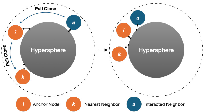
Fig. 1: We random select an item $i$ as the anchor node. The node $k$ is $i^{\prime}$ s nearest neighbor, which is found by the ItemKNN algorithm, and node $a$ has interacted with item $i^{\prime}$ .
图 1: 我们随机选择一个项目 $i$ 作为锚节点。节点 $k$ 是 $i^{\prime}$ 的最近邻,通过 ItemKNN 算法找到,而节点 $a$ 与项目 $i^{\prime}$ 有过交互。
However, while contrastive learning has shown effectiveness in recommendation tasks, it brings new challenges by potentially distancing anchor nodes from their collaborative neighbors. Consequently, some potentially interestaligned neighbors of the user may be treated as false negative samples in the contrastive loss, undermining the optimization of the recommendation model. For example, in Figure 1, for the anchor node item $i,$ , the item $k$ and user $a$ are its nearest and interacted neighbors, respectively. The representations of the anchor node and its nearest neighbors and interacted neighbors should be close to each other in the hyper sphere. The nearest and interacted neighbors are the anchor node’s collaborative neighbors. If the contrastive loss optimizes the recommendation model, it will cause the anchor node $i$ to be far away from the collaborative neighbors, such as the left part in Figure 1. To our best knowledge, few studies have been conducted to address such an issue. In the paper SGL [14], the researchers directly utilize the ranking-based loss function to pull close the anchor node and its interacted neighbors. And in the paper [18], the authors of NCL studied how to find the positive samples of the anchor node based on the cluster method.
然而,尽管对比学习在推荐任务中展现出有效性,它却带来了新的挑战——可能使锚节点(anchor node)远离其协同邻居(collaborative neighbors)。这会导致用户某些潜在兴趣一致的邻居在对比损失(contrastive loss)中被误判为负样本,从而损害推荐模型的优化效果。例如在图1中,对于锚节点商品$i$而言,商品$k$和用户$a$分别是其最近邻和交互邻居。锚节点与其最近邻、交互邻居的表征在超球面上应当彼此接近,这些最近邻和交互邻居共同构成锚节点的协同邻居。若直接采用对比损失优化推荐模型,会导致锚节点$i$远离其协同邻居(如图1左侧所示)。据我们所知,目前仅有少量研究针对该问题展开探索。在论文SGL[14]中,研究者直接采用基于排序的损失函数来拉近锚节点与其交互邻居的距离;而在NCL论文[18]中,作者基于聚类方法研究了如何为锚节点寻找正样本。
Despite numerous strategies proposed to address the challenging task of integrating supervisory signals with contrastive loss, it remains an intricate problem. We propose a potential solution: treating the collaborative neighbors of the anchor node as positive samples in the final objective loss function. This approach aims to optimize the positioning of all nodes’ learned representations in the representation space such that anchor nodes and positive sample nodes are proximate while maximizing the distance from negative sample nodes. Drawing inspiration from the SupCon work [12], we have devised two novel supervised contrastive loss functions for recommendation tasks. These functions have been meticulously designed to guide the backbone model’s optimization more effectively, specifically by focusing on the numerator and denominator of the InfoNCE loss.
尽管已有多种策略被提出用于解决将监督信号与对比损失相结合的难题,但这仍然是一个复杂的问题。我们提出了一种潜在解决方案:在最终目标损失函数中将锚节点的协作邻居视为正样本。该方法旨在优化所有节点学习表征在表征空间中的位置,使得锚节点与正样本节点彼此接近,同时最大化与负样本节点的距离。受SupCon工作[12]启发,我们为推荐任务设计了两种新颖的监督对比损失函数。这些函数经过精心设计,通过聚焦InfoNCE损失的分子和分母,能更有效地指导主干模型的优化。
In the experimental section, we demonstrate the superior performance of LightGCN, the selected backbone model, trained using our proposed loss functions. Evaluated on three real-world datasets—Yelp2018, Gowalla, and AmazonBook—our model outshines the current state-of-the-art contrastive learning method, $\mathrm{SGL,}$ outperforming it by $10.09%,$ $7.09%$ , and $35.36%$ on the $\mathrm{NDCG}@20$ metric, respectively. We also observe that our method shows enhanced utility with smaller temperature values, indicating that the role of negative samples is amplified at lower temperatures. Despite the presence of false negative samples, using some of the user’s nearest neighbors as positive samples for contrastive learning enables us to leverage the advantages of smaller temperature coefficients, thereby offsetting the potential adverse impact of these false samples. Recognizing the potential inaccuracies of algorithm-identified nearest neighbors, we propose strategies to integrate these nearestneighbor users, enhancing the robustness and performance of our model. This approach provides a novel perspective on managing the variability in the quality of positive samples, promising to pave the way for future advancements in the field.
在实验部分,我们展示了采用所提出损失函数训练的骨干模型LightGCN的卓越性能。在Yelp2018、Gowalla和AmazonBook三个真实数据集上的评估表明,我们的模型显著优于当前最先进的对比学习方法 $\mathrm{SGL}$ ,在 $\mathrm{NDCG}@20$ 指标上分别领先 $10.09%$ 、 $7.09%$ 和 $35.36%$ 。我们还发现,该方法在较小温度值下表现出更强的效用,表明负样本在低温环境下作用更为显著。尽管存在假负样本,但将用户的部分最近邻作为对比学习的正样本,使我们能够利用较小温度系数的优势,从而抵消这些假样本的潜在负面影响。考虑到算法识别的最近邻可能存在误差,我们提出了整合这些近邻用户的策略,以增强模型的鲁棒性和性能。这一方法为处理正样本质量波动提供了新思路,有望推动该领域的未来发展。
The contributions of our proposed model can be summarized as follows:
我们提出的模型贡献可总结如下:
- We propose an effective model that leverages multiple positive samples of anchor nodes to guide the update of anchor representations. Theoretical analysis shows that the anchor and multiple negative samples jointly determine the influence of different positive samples.
- 我们提出了一种有效模型,利用锚节点的多个正样本来指导锚表示更新。理论分析表明,锚节点与多个负样本共同决定了不同正样本的影响程度。
- Through experiments, we found that our proposed method performs better with a smaller temperature value. This observation reinforces our hypothesis that by introducing multiple positive samples, we can counteract the detrimental effects of false negative samples and amplify the beneficial effects of true negative samples. This work thus provides new insights into optimizing the performance of contrastive loss by adjusting the temperature value.
- 通过实验,我们发现提出的方法在较小温度值下表现更优。这一观察结果验证了我们的假设:通过引入多个正样本,可以抵消假负样本的有害影响,同时增强真负样本的积极作用。该工作为通过调整温度值优化对比损失性能提供了新思路。
- Given the diversity of positive sample types and their limited quality, we propose several strategies for positive sample selection and evaluate the effectiveness of these strategies. Furthermore, our proposed loss function can naturally accommodate various positive sample types, enhancing the model’s performance.
- 鉴于正样本类型的多样性及其有限质量,我们提出了几种正样本选择策略,并评估了这些策略的有效性。此外,我们提出的损失函数能自然兼容多种正样本类型,从而提升模型性能。
Following, we first introduce the work which is related to our work. Then, to help the readers understand the loss functions we proposed, we introduce preliminary knowledge. Next, we will briefly introduce our proposed loss functions and analyze how they work from a theoretical perspective. Last, we conducted experiments on three realworld datasets, to analyze the performance of our proposed model from many perspectives.
接下来,我们首先介绍与本研究相关的工作。然后,为帮助读者理解我们提出的损失函数,将介绍预备知识。随后,我们将简要介绍所提出的损失函数,并从理论角度分析其工作原理。最后,我们在三个真实数据集上进行了实验,从多个角度分析所提出模型的性能。
2 RELATED WORK
2 相关工作
2.1 Graph Neural Network based Recommend er System
2.1 基于图神经网络 (Graph Neural Network) 的推荐系统
This section focuses on works that use graph neural networks in recommendation tasks. CF based models have been widely used for recommending items to users. Among all collaborative filtering based models, latent factor models perform better than other models [4]. However, the performance of such models is limited because of the data sparsity issue. Since the interactions between users and items can be thought of as a user-item bipartite graph, it makes sense that each user’s or item’s preferences will be affected not only by their first-order neighbors but also by their higher-order neighbors [5], [7], [19], [20]. NGCF is proposed to model such higher-order collaborative filtering signal with the help of Graph Neural Network(GCN) technique [7]. However, as the original user-item interaction matrix is very sparse, the performance of NGCF is also limited because of its heavy parameters and non-linear activation function for each message-passing layer. LightGCN is proposed to address the issue of NGCF, by removing the transform parameters and non-linear activation function of NGCF [5]. As directly utilizing the GCN technique in recommendation tasks may encounter an over-smoothing issue, LRGCCF [8] is proposed to alleviate the issue by concatenating the output representations of all users and items among all message-passing layers. Even though the LightGCN model has shown surprising performance in recom mend ation tasks, it is inefficient because of the multiple message-passing layers. The authors in UltraGCN proposed a model named UltraGCN to approximate the stacking message passing operation of LightGCN with a contrastive loss [21]. It can reduce the inference time of LightGCN, while it is also time-consuming in the training stage as it has to sample a lot of negative samples. Besides modeling the user-item bipartite graph, the graph neural network technique is also utilized in other kinds of recommendation tasks, for example, social recommendation [22], [23], fraud detection [24], review-based recommendation [25] and attribute inference [26].
本节重点介绍在推荐任务中应用图神经网络的研究工作。基于协同过滤(CF)的模型已被广泛用于向用户推荐物品。在所有基于协同过滤的模型中,潜在因子模型表现优于其他模型[4]。然而,由于数据稀疏性问题,此类模型的性能受到限制。由于用户与物品的交互可视为用户-物品二分图,每个用户或物品的偏好不仅会受其一阶邻居影响,还会受高阶邻居影响[5][7][19][20]。NGCF借助图神经网络(GCN)技术对这种高阶协同过滤信号进行建模[7]。但由于原始用户-物品交互矩阵非常稀疏,NGCF因其繁重的参数和每层消息传递的非线性激活函数而性能受限。LightGCN通过移除NGCF的变换参数和非线性激活函数来解决该问题[5]。由于直接在推荐任务中使用GCN技术可能遭遇过平滑问题,LRGCCF[8]通过拼接所有消息传递层中用户和物品的输出表示来缓解该问题。尽管LightGCN在推荐任务中表现出色,但因多层消息传递导致效率低下。UltraGCN的作者提出用对比损失近似LightGCN的堆叠消息传递操作[21],虽能减少推理时间,但训练阶段因需采样大量负样本仍耗时。除建模用户-物品二分图外,图神经网络技术还被应用于其他推荐任务,如社交推荐[22][23]、欺诈检测[24]、基于评论的推荐[25]和属性推断[26]。
In summary, graph convolutional networks have shown great promise in recommendation tasks, particularly in addressing data sparsity issues and encapsulating higherorder collaborative filtering signals. However, these methods also have shortcomings, such as causing oversmoothing problems. How to alleviate these problems and discover more valuable supervisory signals are still under research.
总之,图卷积网络在推荐任务中展现出巨大潜力,尤其在解决数据稀疏问题和捕捉高阶协同过滤信号方面。然而,这些方法也存在缺陷,例如会导致过度平滑问题。如何缓解这些问题并发现更有价值的监督信号仍是研究热点。
2.2 Self-Supervised Learning Technique
2.2 自监督学习技术
Self-supervised learning technique has been widely studied in computer vision [13], [27], [28], [29], natural language processing [30], [31], [32], and data mining areas [33], [34], [35], [36], [37]. There are two branches of the self-supervised learning technique, generative [38], [39] and contrastive [13], [28], [32]. The key idea of the generative self-supervised papers is designing how to reconstruct the corrupted data or predict the input’s missing data. And the key idea of the contrastive self-supervised learning technique is how to pull the two augmented representations of the same anchor node close, and push the anchor node’s representations away from other nodes’ representations. This paper mainly studies applying the self-supervised technique in user-item bipartite graphs. However, the self-supervised techniques which are used in the computer vision and natural language processing areas can not be directly used in the graph data because the structure of the graph data is complex and irregular. Current works mainly studied how to design pretext tasks that require the model to make predictions or solve auxiliary tasks based on the input graph [33], [34], [35], such as graph reconstruction, node attribution prediction, and so on. Due to the sparsity of the user-item rating matrix in the recommendation task, researchers also attempted to use contrastive learning techniques to augment the input data to improve the performance of recommendation tasks such as sequential recommendation [16], [40], session-based recommendation [41], social recommendation [42], review-based recommendation [43], and candidate matching tasks [14], [17], [21].
自监督学习技术在计算机视觉 [13]、[27]、[28]、[29]、自然语言处理 [30]、[31]、[32] 以及数据挖掘领域 [33]、[34]、[35]、[36]、[37] 得到了广泛研究。自监督学习技术主要分为两类:生成式 [38]、[39] 和对比式 [13]、[28]、[32]。生成式自监督论文的核心思想是设计如何重建损坏数据或预测输入的缺失数据,而对比式自监督学习技术的核心思想是如何拉近同一锚节点的两个增强表示,并将锚节点的表示与其他节点的表示推远。本文主要研究将自监督技术应用于用户-物品二分图。然而,由于图数据的结构复杂且不规则,计算机视觉和自然语言处理领域的自监督技术无法直接应用于图数据。当前工作主要研究如何设计前置任务,要求模型基于输入图进行预测或解决辅助任务 [33]、[34]、[35],例如图重建、节点属性预测等。由于推荐任务中用户-物品评分矩阵的稀疏性,研究者还尝试使用对比学习技术增强输入数据,以提升序列推荐 [16]、[40]、基于会话的推荐 [41]、社交推荐 [42]、基于评论的推荐 [43] 以及候选匹配任务 [14]、[17]、[21] 等推荐任务的性能。
In our paper, we mainly focus on the candidate-matching task. In current works, the researchers studied how to augment the representations of the users and items, and how to design contrastive loss to learn a more robust recommendation model [14], [15], [18]. One of the key techniques of utilizing contrastive loss is how to augment the data. In SGL, the authors in SGL proposed three kinds of data augmentations strategies, node dropout, edge dropout, and random walk to augment the original bipartite graph [14]. However, in the paper [44], the authors even found that the simple sampled softmax loss itself is capable of mining hard negative samples to enhance the performance of the recommendation models without data augmentation. As the data augmentation of SGL [14] is time-consuming, the authors in GACL proposed a simple but effective method to augment the representations of the users and items [15], i.e., adding perturbing noise to the representations of the users and items. Some researchers also studied how to utilize positive samples [18]. In this paper NCL [18], the authors cluster the users and items into several clusters, respectively. And for each anchor node, its corresponding cluster is treated as the positive sample. In the paper [45], the authors proposed a whitening-based method to avoid the representations collapse issue, and they argued that the negative samples are not necessary in the model training stage. Besides, some researchers studied how to find the negative samples [46], [47].
在我们的论文中,我们主要关注候选匹配任务。当前研究中,学者们探索了如何增强用户和物品的表示,以及如何设计对比损失来学习更鲁棒的推荐模型 [14][15][18]。使用对比损失的关键技术之一在于数据增强方法。在SGL中,作者提出了三种数据增强策略:节点丢弃、边丢弃和随机游走,用于增强原始二分图 [14]。然而,论文[44]发现即使不进行数据增强,简单的采样softmax损失本身就能挖掘困难负样本来提升推荐模型性能。由于SGL [14]的数据增强耗时较长,GACL的作者提出了一种简单有效的方法来增强用户和物品表示 [15],即对用户和物品表示添加扰动噪声。另有研究者探索了如何利用正样本 [18],在NCL [18]中,作者分别将用户和物品聚类为若干簇,并将每个锚节点对应的簇视为正样本。论文[45]提出基于白化的方法来避免表示坍塌问题,并指出模型训练阶段不一定需要负样本。此外,还有研究专注于负样本挖掘方法 [46][47]。
As our main task is how to design the contrastive loss function to constrain the distance between the anchor node and its collaborative neighbors, to our best knowledge, we found the following two papers, which are related to our work. In the paper [48], the authors further studied the uniformity characteristic of the contrastive loss. They proposed that high uniformity would lead to low tolerance, and make the learned model may push away two samples with similar semantics. Besides, the authors in the paper [49] studied how to utilize the popularity degree information to help the collaborative model automatically adjust the collaborative representations optimization intensity of any user-item pair [49]. The most related work to ours is SupCon [12]. Though we both proposed two kinds of supervised contrastive loss functions, optimizing the loss functions we proposed model can achieve better performance than the ones in the SupCon. The main difference is the design of the numerator and denominator of the InfoNCE loss. The experimental results also show that training the model based on our proposed loss functions could achieve better than training the model based on the SupCon loss. We suppose that compared to the loss function proposed in Supcon, our proposed loss function is more effective in adaptively tuning the weights of all positive samples. In the section on experiments, the experiments also test how well our proposed loss functions work.
我们的主要任务是如何设计对比损失函数来约束锚节点与其协作邻居之间的距离。据我们所知,我们发现以下两篇论文与我们的工作相关。在论文[48]中,作者进一步研究了对比损失的一致性特征。他们提出高一致性会导致低容忍度,使学习到的模型可能推开两个语义相似的样本。此外,论文[49]的作者研究了如何利用流行度信息帮助协作模型自动调整任意用户-物品对的协作表示优化强度[49]。与我们工作最相关的是SupCon[12]。虽然我们都提出了两种监督对比损失函数,但优化我们提出的损失函数模型能比SupCon中的模型获得更好的性能。主要区别在于InfoNCE损失分子和分母的设计。实验结果也表明,基于我们提出的损失函数训练模型比基于SupCon损失训练模型效果更好。我们认为,与Supcon提出的损失函数相比,我们提出的损失函数在自适应调整所有正样本权重方面更有效。在实验部分,实验还测试了我们提出的损失函数的效果。
2.3 Neighbor-based Collaborative Filtering Methods
2.3 基于邻域的协同过滤方法
As we utilize the neighbor-based methods to find nearestneighbors of the anchor node, we would simply introduce the neighbor-based collaborative filtering methods. Following, we will simply introduce several kinds of methods that find the nearest neighbors. Then, we will introduce how to utilize the nearest neighbors to help recommendation task.
在使用基于邻居的方法寻找锚节点的最近邻时,我们将简要介绍基于邻居的协同过滤方法。接下来,我们将简要介绍几种寻找最近邻的方法。然后,我们将介绍如何利用最近邻来辅助推荐任务。
We split the current nearest-neighbors finding methods into the following three categories. First is finding nearest neighbors based on historical records, such as ItemKNN [2], and UserKNN [3]. Second, to find the nearest neighbors of the cold-start users or items, the researchers incorporate more kinds of data, such as text [50], [51], KG [52], and social network [22], [23]. Third, the researchers aim to find the nearest neighbors with the learned embeddings, such as cluster, and most of current works. After getting the nearest neighbors, the data can be used to serve recommendations directly, such as ItemCF [2] and SLIM [1], or enhancing the representations of the items, such as $\mathrm{SVD++}$ [6], Diffnet [22], and so on.
我们将当前的最近邻查找方法分为以下三类。第一类是基于历史记录的最近邻查找,例如ItemKNN [2]和UserKNN [3]。第二类是为冷启动用户或物品寻找最近邻,研究人员引入了更多类型的数据,如文本 [50]、[51]、知识图谱 (KG) [52] 和社交网络 [22]、[23]。第三类是通过学习到的嵌入向量寻找最近邻,例如聚类和当前大多数工作。获取最近邻后,这些数据可直接用于推荐服务,如ItemCF [2]和SLIM [1],或用于增强物品表征,例如$\mathrm{SVD++}$ [6]、Diffnet [22]等。
3 PROBLEM DEFINITION & PRELIMINARY
3 问题定义与初步准备
In this section, we briefly introduce the preliminary knowledge which is related to our proposed model. First, we introduce the key technique of the backbone model LightGCN [5] we use. Then, we introduce how augment the input data and how to achieve the augmented users’ and items’ representations.
在本节中,我们简要介绍与所提出模型相关的预备知识。首先,我们介绍骨干模型 LightGCN [5] 使用的关键技术。接着,我们介绍如何增强输入数据以及如何获得增强后的用户和物品表征。
3.1 Notation & Problem Definition
3.1 符号与问题定义
In this paper, we aim to study how to model different kinds of positive samples of the anchor node when designing the supervised contrastive loss. As the backbone model is the LightGCN [5], we would introduce the data which is used in the training stage. Given the user set $\mathcal{U}(|\mathcal{U}|=m)$ , item set $\nu(|\nu|=n)$ , and the corresponding rating matrix $\mathbf{R},$ where ${\bf R}_{a i}=1$ denotes the user $a$ and item $i$ has interaction, we first construct the bipartite user-item graph ${\mathcal{G}}=({\mathcal{N}},{\mathcal{E}}).$ , where ${\mathcal{N}}=\mathcal{U}\cup\mathcal{V},$ and $\mathcal{E}$ consists of the connected user-item pairs in the rating matrix $\mathbf{R}$ . For any node $i\in\mathcal N$ , $\mathbf{R}_{i}^{+}$ denotes the node $i^{\prime}$ ’s interacted neighbors. Because we treat the anchor nodes’ interacted neighbors and nearest neighbors both as collaborative neighbors, we then introduce how to achieve the nearest neighbors simply. For example, for any anchor node $i\in\mathcal N$ , we use $S_{i}$ to denote its nearest neighbor set. The number $K$ of the nearest neighbors set $S_{i}$ is a hyperparameter, which is predefined in advance. As our proposed loss function is based on the contrastive loss technique, the details about how to augment the input graph and how to get the augmented representations can refer to the following section. The important notations which appear in this paper can refer to Table 1.
本文旨在研究设计监督对比损失时如何对锚节点的各类正样本进行建模。由于主干模型采用LightGCN [5],我们将首先介绍训练阶段使用的数据。给定用户集$\mathcal{U}(|\mathcal{U}|=m)$、物品集$\nu(|\nu|=n)$及对应的评分矩阵$\mathbf{R}$(其中${\bf R}_{a i}=1$表示用户$a$与物品$i$存在交互),我们首先构建二分用户-物品图${\mathcal{G}}=({\mathcal{N}},{\mathcal{E}})$,其中${\mathcal{N}}=\mathcal{U}\cup\mathcal{V}$,$\mathcal{E}$由评分矩阵$\mathbf{R}$中相连的用户-物品对组成。对于任意节点$i\in\mathcal N$,$\mathbf{R}_{i}^{+}$表示节点$i^{\prime}$的交互邻居。由于我们将锚节点的交互邻居和最近邻均视为协同邻居,接下来简要说明最近邻的获取方式:例如对于任意锚节点$i\in\mathcal N$,使用$S_{i}$表示其最近邻集合,该集合的大小$K$作为超参数需预先设定。由于我们提出的损失函数基于对比损失技术,关于输入图增强及增强表征获取的具体方法详见下文。本文重要符号参见表1。
TABLE 1: Notation Table.
| Notation | Description |
| 5 | User-item bipartite graph |
| TheunionoftheusersetZanditemitem | |
| Edge set of the graph g | |
| R | Nodei'sinteractedneighbors |
| Si | Nodei'snearestneighbors |
| 15'5 | The augmentedtwographs |
| H',H" | The representations of all nodes from two views |
| T | The temperature value in the contrastiveloss |
| p | Thedropratiointhedataaugmentationprocess |
表 1: 符号表
| 符号 | 描述 |
|---|---|
| 5 | 用户-物品二分图 |
| 用户集Z与物品集的并集 | |
| 图g的边集 | |
| R | 节点i的交互邻居 |
| Si | 节点i的最近邻居 |
| 15'5 | 增强后的两个图 |
| H', H" | 两个视角下所有节点的表示 |
| T | 对比损失中的温度值 |
| p | 数据增强过程中的丢弃比率 |
predicted rating $\hat{r}_{a i}$ can be calculated with the inner product operation:
预测评分 $\hat{r}_{a i}$ 可通过内积运算计算得出:
$$
\hat{r}{a i}=\mathbf{h}{a}\mathbf{h}_{i}^{\top}
$$
$$
\hat{r}{a i}=\mathbf{h}{a}\mathbf{h}_{i}^{\top}
$$
For the LightGCN model, the model parameters are optimized to minimize the following ranking-based loss $\mathcal{L}_{R}$ :
对于 LightGCN 模型,模型参数通过最小化以下基于排序的损失 $\mathcal{L}_{R}$ 进行优化:
$$
\mathcal{L}{R}=-\sum_{a\in\mathcal{U}}\sum_{i\in\mathbf{R}{a}^{+},j\in\mathbf{R}{a}^{-}}l o g\big(\sigma\big(\hat{r}{a i}-\hat{r}_{a j}\big)\big),
$$
$$
\mathcal{L}{R}=-\sum_{a\in\mathcal{U}}\sum_{i\in\mathbf{R}{a}^{+},j\in\mathbf{R}{a}^{-}}l o g\big(\sigma\big(\hat{r}{a i}-\hat{r}_{a j}\big)\big),
$$
where $\sigma(\cdot)$ is the sigmoid function, $\sigma(x)=1/(1+e^{-x}),{\bf R}{a}^{+}$ denotes the observed items which have interactions with user $^{a,}$ and ${\bf R}_{a}^{-}$ denotes the items which are not connected with the user $a$ .
其中 $\sigma(\cdot)$ 是 sigmoid 函数,$\sigma(x)=1/(1+e^{-x})$,${\bf R}{a}^{+}$ 表示与用户 $a$ 有交互的观测项,${\bf R}_{a}^{-}$ 表示未与用户 $a$ 连接的项。
3.3 Data Augmentation
3.3 数据增强
According to the setting of the model SGL [14], the interaction data should be disturbed first to generate the augmented user-item bipartite graphs $\mathcal{G^{\prime}}$ and $\bar{g}^{\prime\prime}$ . In the original paper of SGL, the authors proposed three kinds of data augmentation strategies, Node Dropout, Edge Dropout, and Random Walk. The first two data augmentation strategies randomly drop the nodes and edges of the input user-item bipartite graph by setting the drop ratio $\rho$ . The corrupted graphs are also called augmented graphs. And the augmented graphs are fixed among all information propagation layers of the GNN-based module. The Random Walk adopts the same strategy as the Edge Dropout to augment the input graph, while at different information propagation layers, the augmented graphs are different. More details can refer to the original paper of SGL [14]. With the augmented graphs, the augmented users’ and items’ representations $\mathbf{H}^{\prime}$ , $\mathbf{H}^{\prime\prime}$ can be learned from these augmented data. Finally, an InfoNCE loss is used to push other nodes’ representations away from the anchor nodes i’s two view representations and pull the two view representations of the same anchor node $i^{.}$ ’s close. The data augmentation strategies which are used in the SGL [14] is also used in our proposed model.
根据模型SGL[14]的设置,应首先扰动交互数据以生成增强的用户-物品二分图$\mathcal{G^{\prime}}$和$\bar{g}^{\prime\prime}$。在SGL原论文中,作者提出了三种数据增强策略:节点丢弃(Node Dropout)、边丢弃(Edge Dropout)和随机游走(Random Walk)。前两种策略通过设置丢弃比率$\rho$,随机丢弃输入用户-物品二分图的节点和边。被破坏的图也称为增强图,且这些增强图在基于GNN模块的所有信息传播层中保持固定。随机游走采用与边丢弃相同的策略来增强输入图,但在不同信息传播层会生成不同的增强图。更多细节可参阅SGL原论文[14]。
利用增强后的图,可以从这些增强数据中学习到用户和物品的增强表示$\mathbf{H}^{\prime}$、$\mathbf{H}^{\prime\prime}$。最终使用InfoNCE损失函数,将其他节点的表示推离锚节点$i$的两个视图表示,同时拉近同一锚节点$i^{.}$的两个视图表示。我们提出的模型也采用了SGL[14]中使用的数据增强策略。
4 NEIGHBORHOOD-ENHANCED SUPERVISED CONTRASTIVE LEARNING
4 邻域增强的监督对比学习
3.2 Model-based Method: LightGCN
3.2 基于模型的方法:LightGCN
The main idea of the LightGCN model is modeling the user-item high-order collaborative signal through the GCN network. Given the user-item bipartite graph $\breve{\boldsymbol{\mathcal{G}}}=(\mathcal{N},\mathcal{E}),$ , the LightGCN model can learn the users’ and items’ representations through $K$ iteration layers. At the $k$ -th layer, the learned users’ and items’ representations $\mathbf{H}^{k}$ can be treated as containing their $k$ -hop neighbors’ information. To alleviate the over-smoothing issue in GNN-based models [8], the representations of all nodes among all propagation layers are concatenated with:
LightGCN模型的核心思想是通过GCN网络建模用户-物品的高阶协同信号。给定用户-物品二分图$\breve{\boldsymbol{\mathcal{G}}}=(\mathcal{N},\mathcal{E})$,LightGCN模型可通过$K$个迭代层学习用户和物品的表征。在第$k$层时,学习到的用户和物品表征$\mathbf{H}^{k}$可视为包含其$k$跳邻居信息。为缓解基于GNN模型的过平滑问题[8],所有传播层中节点的表征通过以下方式拼接:
$$
\mathbf{H}=[\mathbf{H}^{0},\mathbf{H}^{1},...,\mathbf{H}^{K}].
$$
$$
\mathbf{H}=[\mathbf{H}^{0},\mathbf{H}^{1},...,\mathbf{H}^{K}].
$$
The concatenated representations $\mathbf{H}$ are also treated as the final representations of all users and items. For user $a$ and item $i,$ their representations are denoted as $\mathbf{h}{a}$ and $\mathbf{h}_{i},$ respectively. Then, for any pair of user-item $(a,i)$ , their
拼接后的表示 $\mathbf{H}$ 也被视为所有用户和物品的最终表示。对于用户 $a$ 和物品 $i$,它们的表示分别记为 $\mathbf{h}{a}$ 和 $\mathbf{h}_{i}$。那么,对于任意用户-物品对 $(a,i)$,它们的
This paper aims to modify the traditional contrastive learning technique to incorporate different kinds of positive samples in recommendation tasks. We argue that when constructing the contrastive loss for the anchor node $i,$ not only its’ representations of two views should be treated as its positive samples, but also the representations of its collaborative neighbors. The challenge we address is how to model multiple positive samples of the anchor node. Inspired by the SupCon [12], which also focuses on designing the supervised contrastive loss function to model the positive samples. We proposed two unique supervised contrastive loss functions Neighborhood-Enhanced Supervised Contrastive Loss (NESCL), with $\mathit{\Omega}^{\prime\prime}\mathrm{in}^{\prime\prime}$ -version and “out”-version. The two loss functions can refer to Equation (5) and Equation (6), respectively. The overall framework about how our proposed two unique loss functions work can refer to Figure 2. We treat the LightGCN [5] as the backbone model and adopt the same data augmentation strategy as SGL [14].
本文旨在改进传统的对比学习技术,以在推荐任务中融入不同类型的正样本。我们认为,在构建锚节点 $i$ 的对比损失时,不仅应将其两个视图的表示视为正样本,还应将其协同邻居的表示纳入正样本。我们解决的挑战是如何建模锚节点的多个正样本。受 SupCon [12] 启发(该方法同样专注于设计监督对比损失函数来建模正样本),我们提出了两种独特的监督对比损失函数:邻域增强监督对比损失 (Neighborhood-Enhanced Supervised Contrastive Loss, NESCL),包括 $\mathit{\Omega}^{\prime\prime}\mathrm{in}^{\prime\prime}$ 版本和 "out" 版本。这两个损失函数分别对应公式 (5) 和公式 (6),整体框架可参见图 2。我们以 LightGCN [5] 作为主干模型,并采用与 SGL [14] 相同的数据增强策略。
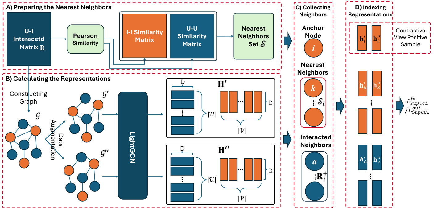
Fig. 2: The overall framework for utilizing our proposed Neighborhood-Enhanced Supervised Contrastive Loss (NESCL). There are four parts, A) It is used to calculate the user-user similarity matrix and item-item similarity matrix based on the user-item interacted matrix R. B) It denotes how to get the two representation matrix ${\bf H}^{\prime}\in\mathbb{R}^{(|\mathcal{U}|+|\mathcal{V}|)\times D}$ and augmented representations $\mathbf{H}^{\prime\prime}\in\mathbb{R}^{(|\mathcal{U}|+|\mathcal{V}|)\times D}$ of all users and item. The $\mathcal{G^{\prime}}$ and $\mathcal{G}^{\prime\prime}$ denote the two augmented graphs, respectively. C) For any anchor node(item $i\ddot{\jmath}{\perp}$ ), it is necessary to collect its nearest neighbors $S_{i}$ based on the item-item similarity matrix and its interacted neighbors based on the user-item interacted matrix. D) Before calculating the supervised collaborative rce op nrt ers aest n itv a et iloons s m fuat nrc it xi.o nAss $\mathcal{L}{N E S C L}^{i n}$ eostr $\mathcal{L}_{N E S C L}^{o u t},$ wane ds hi not uel rd a catlesdo innedigexh btohres raerper evseernyt act lie o an rs ionf tahlil s ufsiegrusr ea,n dw eit ehimgsh flirgohmt tthhee contrastive view positive sample of the anchor node in this figure.
图 2: 使用我们提出的邻域增强监督对比损失 (NESCL) 的整体框架。包含四个部分:A) 基于用户-物品交互矩阵 R 计算用户-用户相似度矩阵和物品-物品相似度矩阵。B) 展示如何获得所有用户和物品的两个表示矩阵 ${\bf H}^{\prime}\in\mathbb{R}^{(|\mathcal{U}|+|\mathcal{V}|)\times D}$ 及增强表示 $\mathbf{H}^{\prime\prime}\in\mathbb{R}^{(|\mathcal{U}|+|\mathcal{V}|)\times D}$。其中 $\mathcal{G^{\prime}}$ 和 $\mathcal{G}^{\prime\prime}$ 分别表示两个增强图。C) 对于任意锚节点 (物品 $i\ddot{\jmath}{\perp}$),需要基于物品-物品相似度矩阵收集其最近邻 $S_{i}$,以及基于用户-物品交互矩阵收集其交互邻居。D) 在计算监督协作对比损失 $\mathcal{L}{N E S C L}^{i n}$ 和 $\mathcal{L}_{N E S C L}^{o u t}$ 之前,需要整合所有信号,图中高亮部分表示该锚节点在对比视图中的正样本。
The following section will first introduce the preparation for calculating the NESCL. Then, we will introduce the forward calculation process. Last, we will introduce the details of the designed $N E S C L,$ and analyze how it dynamically weighs the importance of different kinds of positive samples from the theoretical perspective. Finally, we will discuss the complexity of our proposed model and the related model SGL.
以下部分将首先介绍计算NESCL的准备工作。接着,我们将介绍前向计算过程。最后,我们将详细阐述设计的$NESCL$,并从理论角度分析其如何动态权衡不同类型正样本的重要性。最终,我们将讨论所提模型及相关模型SGL的复杂度。
4.1 Preparation for Calculating NESCL
4.1 计算NESCL的准备工作
This section will introduce how to find the anchor node $i^{\prime}$ ’s nearest neighbors. There are two kinds of memorybased methods used in our work, user-based [3] and itembased [2]. In this section, we will take the item-based method ItemKNN as an example, introducing how to generate recommendations based on memory-based methods. The recommendation generation procedure can be divided into two sub-procedures. First is calculating the similarity $s i m(i,j)$ between any two items $i$ and $j$ :
本节将介绍如何找到锚节点 $i^{\prime}$ 的最近邻。我们的工作中使用了两种基于内存的方法:基于用户的方法 [3] 和基于物品的方法 [2]。本节将以基于物品的 ItemKNN 方法为例,介绍如何基于内存方法生成推荐。推荐生成过程可分为两个子步骤:首先计算任意两个物品 $i$ 和 $j$ 之间的相似度 $sim(i,j)$:
nearest neighbors. And we use $S_{i}$ to denote node $i^{.}$ ’s nearest neighbors set.
最近邻。我们用 $S_{i}$ 表示节点 $i^{.}$ 的最近邻集合。
4.2 Model Forward Process
4.2 模型前向过程
In the model forward process, we will introduce how to achieve the representations of the anchor node and its positive samples. Then, these achieved representations would be used to calculate the supervised collaborative contrastive loss functions $\mathcal{L}{N E S C L}^{i n}$ and $\mathcal{L}{N E S C L}^{o u t}$ . Given the input graph $\mathcal{G},$ it would be augmented twice to get two augmented graphs $\mathcal{G^{\prime}}$ and $\mathcal{G}^{\prime\prime}$ , with one kind of the data augmentation strategies Node Dropout, Edge Dropout, and Random Walk with drop ratio $\rho$ . Then, based on the same backbone model LightGCN, we can get two representation matrices, $\mathbf{H}^{\prime}$ and $\mathbf{H}^{\prime\prime}$ . Then, for any anchor node $i,$ we index the representations of its nearest neighbors $S_{i}$ and interacted neighbors ${\bf R}{i}^{+}$ . Following, we will introduce the designed loss functions $\mathcal{L}{N E S C L}^{i n}$ and $\mathcal{L}_{N E S C L}^{o u t}$ based on the indexed representations.
在模型前向过程中,我们将介绍如何实现锚节点及其正样本的表示。随后,这些获得的表示将用于计算监督协同对比损失函数 $\mathcal{L}{N E S C L}^{i n}$ 和 $\mathcal{L}{N E S C L}^{o u t}$。给定输入图 $\mathcal{G}$,通过两次增强得到两个增广图 $\mathcal{G^{\prime}}$ 和 $\mathcal{G}^{\prime\prime}$,采用的增强策略包括节点丢弃 (Node Dropout)、边丢弃 (Edge Dropout) 和随机游走 (Random Walk),丢弃比例为 $\rho$。接着,基于相同的骨干模型 LightGCN,可获得两个表示矩阵 $\mathbf{H}^{\prime}$ 和 $\mathbf{H}^{\prime\prime}$。对于任意锚节点 $i$,我们索引其最近邻 $S_{i}$ 和交互邻居 ${\bf R}{i}^{+}$ 的表示。下文将基于索引到的表示,介绍设计的损失函数 $\mathcal{L}{N E S C L}^{i n}$ 和 $\mathcal{L}_{N E S C L}^{o u t}$。
$$
s i m(i,j)=\frac{|\mathbf{R}{i}^{+}\cap\mathbf{R}{j}^{+}|}{\sqrt{|\mathbf{R}{i}^{+}||\mathbf{R}_{j}^{+}|}},
$$
$$
s i m(i,j)=\frac{|\mathbf{R}{i}^{+}\cap\mathbf{R}{j}^{+}|}{\sqrt{|\mathbf{R}{i}^{+}||\mathbf{R}_{j}^{+}|}},
$$
4.3 Details of NESCL
4.3 NESCL 详情
where $|\mathbf{R}{i}^{+}\cap\mathbf{R}{j}^{+}|$ denote how many common interacted users of the items $i$ and $j$ . $|{\bf R}{i}^{+}|$ and $|{\bf R}_{j}^{+}|$ denote the degrees of items $i$ and $j$ , respectively. As the item set $\nu$ is very large, to reduce the following time-consuming in generating recommendations, for each item $i,$ we treat the top-K items which have the largest $s i m(i,j)$ values as $i^{\cdot}$ ’s
其中 $|\mathbf{R}{i}^{+}\cap\mathbf{R}{j}^{+}|$ 表示物品 $i$ 和 $j$ 的共同交互用户数,$|{\bf R}{i}^{+}|$ 和 $|{\bf R}_{j}^{+}|$ 分别表示物品 $i$ 和 $j$ 的度数。由于物品集 $\nu$ 规模庞大,为降低后续推荐生成的计算开销,对于每个物品 $i$,我们将其相似度 $sim(i,j)$ 值最高的前K个物品视为 $i$ 的
The main idea of our proposed loss function is, by optimizing the supervised contrastive loss function, the learned anchor’s representation should be not only apart from other negative nodes but also close to its collaborative neighbors, i.e., nearest neighbors and interacted neighbors. For any anchor node $i,$ given its two views of representations $\mathbf{h}{i}^{\prime}$ and $\mathbf{h}{i}^{\prime\prime}.$ , the representations of its nearest neighbors $\mathbf{h}{k}^{\prime},k\in S_{i},$ and the representations of its interacted neighbors ${\bf h}{a}^{\prime},a\in$ ${\bf R}_{i}^{+}$ , we can get following two kinds of supervised loss functions LNESCL and LoNuEt SCL. They are designed to optimize the backbone recommendation model and will work independently. Our motivation for designing these two loss functions is to investigate the impact of different types of polynomial fusion methods on model optimization under the InfoNCE-based loss function.
我们提出的损失函数的核心思想是,通过优化监督对比损失函数,学习到的锚点表征不仅应远离其他负样本节点,还应靠近其协作邻居(即最近邻和交互邻居)。对于任意锚点节点 $i$,给定其两个视角的表征 $\mathbf{h}{i}^{\prime}$ 和 $\mathbf{h}{i}^{\prime\prime}$,其最近邻的表征 $\mathbf{h}{k}^{\prime},k\in S_{i}$,以及其交互邻居的表征 ${\bf h}{a}^{\prime},a\in$ ${\bf R}_{i}^{+}$,可得到以下两种监督损失函数 LNESCL 和 LoNuEt SCL。这些函数专为优化骨干推荐模型设计,将独立发挥作用。我们设计这两个损失函数的动机,是研究基于 InfoNCE 的损失函数框架下,不同类型多项式融合方法对模型优化的影响。
The equations of them are:
它们的方程为:
$$
\begin{array}{l}{{\displaystyle{\mathcal L}{N E S C L}^{i n}=-\sum_{i\in\mathcal{N}}l o g\frac{e x p({\bf h}{i}^{\prime}({\bf h}{i}^{\prime\prime})^{\top}/\tau)}{\sum_{j\in\mathcal{N}}e x p({\bf h}{i}^{\prime}({\bf h}{j}^{\prime\prime})^{\top}/\tau)}}}\ {{\displaystyle-\sum_{i\in\mathcal{N}}l o g\sum_{k\in{\mathcal{S}{i}}}\frac{s i m(i,k)e x p({\bf h}{k}^{\prime}({\bf h}{i}^{\prime\prime})^{\top}/\tau)}{\sum_{j\in\mathcal{N}}e x p({\bf h}{k}^{\prime}({\bf h}{j}^{\prime\prime})^{\top}/\tau)}}}\ {{\displaystyle~-\sum_{i\in\mathcal{N}}l o g\sum_{a\in{\bf R}{i}^{+}}\frac{e x p({\bf h}{a}^{\prime}({\bf h}{i}^{\prime\prime})^{\top}/\tau)}{\sum_{j\in\mathcal{N}}e x p({\bf h}{a}^{\prime}({\bf h}_{j}^{\prime\prime})^{\top}/\tau)}},}\end{array}
$$
and
和
$$
\begin{array}{r}{\mathcal{L}{N E S C L}^{o u t}=-\displaystyle\sum_{i\in\mathcal{N}}l o g(\frac{e x p(\mathbf{h}{i}^{\prime}(\mathbf{h}{i}^{\prime\prime})^{\top}/\tau)}{\sum_{j\in\mathcal{N}}e x p(\mathbf{h}{i}^{\prime}(\mathbf{h}{j}^{\prime\prime})^{\top}/\tau)}}\ {+\displaystyle\sum_{k\in\mathcal{S}{i}}\frac{s i m(i,k)e x p(\mathbf{h}{k}^{\prime}(\mathbf{h}{i}^{\prime\prime})^{\top}/\tau)}{\sum_{j\in\mathcal{N}}e x p(\mathbf{h}{k}^{\prime}(\mathbf{h}{j}^{\prime\prime})^{\top}/\tau)}}\ {+\displaystyle\sum_{a\in\mathbf{R}{i}^{+}}\frac{e x p(\mathbf{h}{a}^{\prime}(\mathbf{h}{i}^{\prime\prime})^{\top}/\tau)}{\sum_{j\in\mathcal{N}}e x p(\mathbf{h}{a}^{\prime}(\mathbf{h}_{j}^{\prime\prime})^{\top}/\tau)}),}\end{array}
$$
where the notation $s i m(a,i)$ denotes the similarity between the node $a$ and $i,$ , it is provided by the memory-based methods. And the number of the $S_{i}$ is predefined with $K$ . We will give more experimental results of K and the influence of neighbors in the experimental part.
其中符号 $sim(a,i)$ 表示节点 $a$ 和 $i$ 之间的相似度,该值由基于记忆的方法提供。$S_{i}$ 的数量由 $K$ 预先定义。我们将在实验部分给出更多关于 $K$ 的实验结果以及邻居节点的影响。
Though these two kinds of loss functions seem similar, they play different roles in weighing the importance of different kinds of positive samples. In the following section, we will analyze the difference and how they weigh the difference of different kinds of positive samples from the gradient perspective.
虽然这两种损失函数看起来相似,但它们在权衡不同类型正样本重要性时发挥着不同作用。在下一节中,我们将从梯度角度分析它们的差异,以及它们如何权衡不同类型正样本的区别。
4.4 Analysis of Our Proposed Loss Functions from the Gradient Perspective
4.4 从梯度角度分析我们提出的损失函数
4.4.1 Analysis of the “in”-version Loss Function $\mathcal{L}{N E S C L}^{i n}$ To better study the proposed contrastive loss function, first, we use the $\mathcal{L}_{N E S C L}^{i\dot{n}}$ to the following equation:
4.4.1 "in"版本损失函数 $\mathcal{L}{N E S C L}^{i n}$ 分析
为了更好地研究提出的对比损失函数,我们首先将 $\mathcal{L}_{N E S C L}^{i\dot{n}}$ 应用于以下方程:
$$
\begin{array}{r}{\mathcal{L}{N E S C L}^{i n}=-l o g\frac{e x p(\mathbf{h}{i}^{\prime}(\mathbf{h}{i}^{\prime\prime})^{\top}/\tau)}{\sum_{j\in\mathcal{N}}e x p(\mathbf{h}{i}^{\prime}(\mathbf{h}{j}^{\prime\prime})^{\top}/\tau)}}\ {-l o g\frac{e x p(\mathbf{h}{k}^{\prime}(\mathbf{h}{i}^{\prime\prime})^{\top}/\tau)}{\sum_{j\in\mathcal{N}}e x p(\mathbf{h}{k}^{\prime}(\mathbf{h}{j}^{\prime\prime})^{\top}/\tau)}}\ {-l o g\frac{e x p(\mathbf{h}{a}^{\prime}(\mathbf{h}{i}^{\prime\prime})^{\top}/\tau)}{\sum_{j\in\mathcal{N}}e x p(\mathbf{h}{a}^{\prime}(\mathbf{h}_{j}^{\prime\prime})^{\top}/\tau)},}\end{array}
$$
Then, we calculate the gradient from LiNnESCL to the anchor node $i^{\cdot}$ ’s representation $\mathbf{h}_{i}^{\prime\prime}$ . We can get the following equation:
然后,我们计算从LiNnESCL到锚节点$i^{\cdot}$的表示$\mathbf{h}_{i}^{\prime\prime}$的梯度。可以得到以下等式:
$$
\frac{\partial\mathcal{L}{N E S C L}^{i n}}{\partial\mathbf{h}{i}^{\prime\prime}}=\underbrace{\lambda_{i}^{i n}\mathbf{h}{i}^{\prime}}{S G L}+\underbrace{\lambda_{k}^{i n}\mathbf{h}{k}^{\prime}+\lambda_{a}^{i n}\mathbf{h}{a}^{\prime}}_{\mathrm{Neighborhood-Enhanced}}.
$$
$$
\frac{\partial\mathcal{L}{N E S C L}^{i n}}{\partial\mathbf{h}{i}^{\prime\prime}}=\underbrace{\lambda_{i}^{i n}\mathbf{h}{i}^{\prime}}{S G L}+\underbrace{\lambda_{k}^{i n}\mathbf{h}{k}^{\prime}+\lambda_{a}^{i n}\mathbf{h}{a}^{\prime}}_{\mathrm{Neighborhood-Enhanced}}.
$$
According to the analysis of SGL [14], we highlight the difference between our proposed loss function and the loss function in SGL. From the above formula, we can find, with the help of the Neighborhood-Enhanced term, the anchor node’s embedding $\mathbf{h}{i}^{\prime\prime}$ is decided by the positive samples $\mathbf{h}{i}^{\prime},$ ${\bf{h}}{k}^{\prime},$ and $\mathbf{h}_{a}^{\prime}$ simultaneously. It is one of the reasons why our proposed loss function can better guide the optimization of the backbone model.
根据SGL [14]的分析,我们强调所提出的损失函数与SGL中损失函数的区别。从上述公式可以看出,在邻域增强项 (Neighborhood-Enhanced term) 的辅助下,锚节点嵌入 $\mathbf{h}{i}^{\prime\prime}$ 由正样本 $\mathbf{h}{i}^{\prime}$、${\bf{h}}{k}^{\prime}$ 和 $\mathbf{h}_{a}^{\prime}$ 共同决定。这正是我们提出的损失函数能更好指导主干模型优化的原因之一。
Second, the influence capacity $\lambda_{i}^{i n},\lambda_{k}^{i n},$ and $\lambda_{a}^{i n}$ of different positive samples are decided by the anchor node’s representation $\mathbf{h}{i}^{\prime\prime}$ and many negative samples $(\mathbf{h}{j}^{\prime\prime},j\in\mathcal{N},j\\\neq i)$ . It makes the computation of the influence capacity more accurate. For example, the value $\lambda_{k}^{i n}$ can be calculated with:
其次,不同正样本的影响能力 $\lambda_{i}^{in}$、$\lambda_{k}^{in}$ 和 $\lambda_{a}^{in}$ 由锚节点的表示 $\mathbf{h}{i}^{\prime\prime}$ 和多个负样本 $(\mathbf{h}{j}^{\prime\prime},j\in\mathcal{N},j\\\neq i)$ 共同决定。这使得影响能力的计算更为精确。例如,$\lambda_{k}^{in}$ 的值可通过以下方式计算:
$$
\lambda_{k}^{i n}=\frac{1}{\tau}(\frac{-\sum_{j\in\mathcal{N},j\not=i}e x p(\mathbf{h}{k}^{'}(\mathbf{h}{j}^{'\prime})^{\top}/\tau)}{e x p(\mathbf{h}{k}^{'}(\mathbf{h}{i}^{'\prime})^{\top}/\tau)+\sum_{j\in\mathcal{N},j\not=i}e x p(\mathbf{h}{k}^{'}(\mathbf{h}_{j}^{'\prime})^{\top}/\tau)}).
$$
4.4.2 Analysis of the “out”-version Loss Function $\mathcal{L}{N E S C L}^{o u t}$ Similar to the analysis in the last subsection, we adopt the same method to analyze the loss function $\mathcal{L}{N E S C L}^{o u t}$ . By calculating the gradient of LoNuEt SCL to the node i’s auxiliary view $\mathbf{h}_{i}^{\prime\prime}$ , we can get:
4.4.2 "out"版本损失函数 $\mathcal{L}{N E S C L}^{o u t}$ 分析
与上一小节的分析类似,我们采用相同方法分析损失函数 $\mathcal{L}{N E S C L}^{o u t}$。通过计算LoNuEt SCL对节点i辅助视图 $\mathbf{h}_{i}^{\prime\prime}$ 的梯度,可得:
$$
\frac{\partial\mathcal{L}{N E S C L}^{o u t}}{\partial\mathbf{h}{i}^{\prime\prime}}=\lambda_{i}^{o u t}\mathbf{h}{i}^{\prime}+\lambda_{k}^{o u t}\mathbf{h}{k}^{\prime}+\lambda_{a}^{o u t}\mathbf{h}_{a}^{\prime}.,
$$
$$
\frac{\partial\mathcal{L}{N E S C L}^{o u t}}{\partial\mathbf{h}{i}^{\prime\prime}}=\lambda_{i}^{o u t}\mathbf{h}{i}^{\prime}+\lambda_{k}^{o u t}\mathbf{h}{k}^{\prime}+\lambda_{a}^{o u t}\mathbf{h}_{a}^{\prime}.,
$$
According to the above formula, we can get the same conclusion as the $\mathcal{L}{N E S C L}^{i n}$ . And the difference between these two kinds of loss functions is the calculated influence capacity of different positive samples. Compared with the $\prime\prime\mathrm{in}^{\prime\prime}$ -version loss function, the computation of the “out”- version would be more complex. As the formula of the $\lambda_{i}^{o u t}$ , $\lambda_{k}^{o u t}$ , and $\lambda_{a}^{o u t}$ are pretty complex, we would not expand them here. Please refer to Appendix sections A.1 and A.2 for more details.
根据上述公式,我们可以得出与$\mathcal{L}{N E S C L}^{i n}$相同的结论。这两种损失函数的区别在于对不同正样本影响能力的计算方式。与"in"版本损失函数相比,"out"版本的计算会更加复杂。由于$\lambda_{i}^{o u t}$、$\lambda_{k}^{o u t}$和$\lambda_{a}^{o u t}$的公式相当复杂,此处不再展开说明,详见附录章节A.1和A.2。
从公式中,我们得出两点观察。首先,$\lambda_{i}^{o u t}$ 的值应小于 $\lambda_{i}^{i n}$。其次,与 $\lambda_{i}^{i n}$ 相比,$\lambda_{i}^{o u t}$ 的值不仅受其对应正样本 $\mathbf{h}{i.}^{\prime}$ 的距离影响,还受其他正样本 ${\bf{h}}{k}^{\prime}$ 和 $\mathbf{h}_{a}^{\prime}$ 的影响。我们将在实验部分评估这两种损失函数的性能。
4.5 Overall Loss Functions of Our Proposed Model
4.5 我们提出模型的总体损失函数
In this section, we introduce the overall loss function of our proposed model. Although the supervised collaborative contrastive loss we proposed can utilize the information of different kinds of positive samples in the training stage, when conducting experiments, we found that the loss function $\mathcal{L}_{R}$ in Equation (3) is also helpful. We suppose that the two kinds of loss functions can provide different kinds of capacity to pull the anchor node and the positive samples close in the representation space. Thus, the overall loss functions of our proposed model are:
在本节中,我们将介绍所提出模型的总体损失函数。尽管我们提出的监督协作对比损失能够在训练阶段利用不同类型正样本的信息,但在实验过程中发现,公式(3)中的损失函数$\mathcal{L}_{R}$同样具有积极作用。我们认为这两种损失函数能够提供不同的能力,将锚节点与正样本在表征空间中拉近。因此,我们提出的模型总体损失函数为:
$$
\begin{array}{r}{\mathcal{L}{\mathcal{O}}^{i n}=\mathcal{L}{R}+\alpha\mathcal{L}{N E S C L}^{i n},}\ {\mathcal{L}{\mathcal{O}}^{o u t}=\mathcal{L}{R}+\alpha\mathcal{L}_{N E S C L}^{o u t},}\end{array}
$$
where $\alpha$ is a hyper-parameter to balance the importance of the two kinds of loss functions. Larger $\alpha$ means the corresponding loss plays a more important role in the training stage.
其中 $\alpha$ 是一个超参数,用于平衡两种损失函数的重要性。较大的 $\alpha$ 意味着对应的损失在训练阶段扮演更重要的角色。
4.6 Time Complexity
4.6 时间复杂度
In this subsection, we mainly analyze the time complexity when utilizing our proposed loss functions. The overall framework contains the following modules, data preparation, data augmentation, graph convolution, ranking-based loss calculation, and supervised collaborative contrastive loss calculation. As the data augmentation, graph convolution, and ranking-based loss calculation modules are the same as the SGL model, we wouldn’t discuss them here.
在本小节中,我们主要分析使用我们提出的损失函数时的时间复杂度。整体框架包含以下模块:数据准备、数据增强、图卷积、基于排序的损失计算和监督协作对比损失计算。由于数据增强、图卷积和基于排序的损失计算模块与SGL模型相同,这里不再讨论。
The time-consuming procedure for the nearest neighbors finding operation is calculating the user-user similarity and item-item similarity matrices. Its time complexity is $O(|\mathcal{U}||\mathcal{U}|)+O(|\mathcal{V}||\mathcal{V}|)$ . Though the time complexity is high, we only calculate the similarity matrices once. However, in practical applications, we may use different algorithms to discover nearest neighbors with varying time complexities. This step should be considered as a part of the data preparation stage, and thus, we will not discuss its impact on the training complexity of our model.
寻找最近邻操作的耗时过程在于计算用户-用户相似度和物品-物品相似度矩阵。其时间复杂度为 $O(|\mathcal{U}||\mathcal{U}|)+O(|\mathcal{V}||\mathcal{V}|)$ 。尽管时间复杂度较高,但我们仅需计算一次相似度矩阵。然而在实际应用中,可能会采用不同算法来发现最近邻,这些算法具有各异的时间复杂度。此步骤应被视为数据准备阶段的一部分,因此我们将不讨论其对模型训练复杂度的影响。
should be the same. And we taLkeN EthSeC The time complexity of the $\mathcal{L}{N E S C L}^{i n}$ $\mathcal{L}{N E S C L}^{i n}$ and $\mathcal{L}{N E S C L}^{o u t}$ NaEsS CaLn example. For the first term in Equation (5), we can easily find that the complexity of the numerator and denominator should be $O(|\mathcal{N}|\bar{D})$ and $O(|\mathcal{N}||\mathcal{N}|D).$ , respectively. As we only treat other nodes in the batch as the negative samples, the time complexity of the Thus, the time complexity of the denominator can be corrected as $O(|\mathcal{N}|B D))$ , where $B$ is the batch size. Similarly, the time complexity of the second term should be $(O(K|\mathcal{N}|D)+O(K|\mathcal{N}|B D))$ , where $K$ is the number of nearest neighbors for each anchor node $i$ . However, in practice, we found that randomly selecting one nearest neighbor from the neighbor set $S_{i}$ may achieve better performance. Thus, the time complexity of the second term can be reduced to $(O(|\mathcal{N}|D)+\hat{O}(|\mathcal{N}|B D))$ . For the third term in Equation (5), the time complexity should be $({\cal O}(|\mathcal{E}|{\cal D})+{\cal O}(\widehat{2}|\mathcal{E}|{\cal B}{\cal D})).$ , the number 2 means all useritem pairs would appear twice in the third term calculation procedure. The overall supervised collaborative contrastive loss function is $O(|\mathcal{N}|D(\hat{2}+2B))s+O(|\mathcal{E}|D(1+2B))s$ .
应该是相同的。我们讨论 $\mathcal{L}{N E S C L}^{i n}$ 和 $\mathcal{L}{N E S C L}^{o u t}$ 的时间复杂度。以 $\mathcal{L}{N E S C L}^{i n}$ 为例,对于公式 (5) 中的第一项,可以很容易发现分子和分母的复杂度分别为 $O(|\mathcal{N}|\bar{D})$ 和 $O(|\mathcal{N}||\mathcal{N}|D)$。由于我们仅将批次中的其他节点作为负样本,因此分母的时间复杂度可修正为 $O(|\mathcal{N}|B D))$,其中 $B$ 是批次大小。类似地,第二项的时间复杂度应为 $(O(K|\mathcal{N}|D)+O(K|\mathcal{N}|B D))$,其中 $K$ 是每个锚节点 $i$ 的最近邻数量。然而在实际中,我们发现从邻居集 $S_{i}$ 中随机选择一个最近邻可能获得更好的性能,因此第二项的时间复杂度可降低至 $(O(|\mathcal{N}|D)+\hat{O}(|\mathcal{N}|B D))$。对于公式 (5) 中的第三项,其时间复杂度为 $({\cal O}(|\mathcal{E}|{\cal D})+{\cal O}(\widehat{2}|\mathcal{E}|{\cal B}{\cal D}))$,数字 2 表示所有用户-项目对会在第三项计算过程中出现两次。整体监督式协作对比损失函数的时间复杂度为 $O(|\mathcal{N}|D(\hat{2}+2B))s+O(|\mathcal{E}|D(1+2B))s$。
5 EXPERIMENT
5 实验
In the experiment section, we aim to answer the following two questions.
在实验部分,我们旨在回答以下两个问题。
RQ1: Can our proposed supervised loss functions help the backbone model perform better?
RQ1: 我们提出的监督损失函数能否帮助骨干模型提升性能?
TABLE 2: Time Complexity of the Overall Framework for Our Proposed Loss Function and SGL. ( $D$ denotes the vector dimension size, $\rho$ is the data drop ratio in the data augmentation procedure, $s$ is the training epoch number, $B$ is the batch size, and $L$ is the GNN propagation layer number.)
表 2: 我们提出的损失函数和SGL整体框架的时间复杂度。 ( $D$ 表示向量维度大小, $\rho$ 是数据增强过程中的数据丢弃比例, $s$ 是训练周期数, $B$ 是批次大小, $L$ 是GNN传播层数。)
| 组件 | SGL | NESCL |
|---|---|---|
| AdjacencyMatrix | O(4p | ε |
| GraphConvolution | O(2(1+2p)||LD)s | |
| BPRLoSS | O(2 | ε |
| Self-supervisedLoss | O(|N[D(1 + B)s) | |
| SupervisedCollaborative ContrastiveLoss | O(|N|D(2 + 2B))s + O(ε|D(1 + 2B))s |
RQ2: How about the performance of the backbone model under variants of our proposed loss functions?
RQ2: 骨干模型在我们提出的不同损失函数变体下的性能如何?
Following, we first introduce the experiment settings, and then we will answer the above questions individually. As there are some hyper-parameters not important for verifying the effectiveness of our proposed loss function, we would report the results that are related to them in Appendix Section B.
接下来,我们首先介绍实验设置,然后逐一回答上述问题。由于部分超参数对于验证我们提出的损失函数的有效性并不重要,相关结果将在附录B节中汇报。
5.1 Datasets and Metrics
5.1 数据集与评估指标
We conduct experiments based on three public real-world datasets, Yelp2018, Gowalla, and Amazon-Book, which are provided by the authors of LightGCN [5] in the link4. These datasets contain the user-item interacted records. The statistics of these datasets can refer to Table 3. To keep the results the same as the authors reported in these works [5], [14], [21], [53], we also utilize the original format of the provided datasets without any modification.
我们基于三个公开的真实世界数据集 Yelp2018、Gowalla 和 Amazon-Book 进行实验,这些数据集由 LightGCN [5] 的作者在链接4中提供。这些数据集包含用户-物品交互记录。数据集的统计信息可参考表 3。为了保持结果与作者在这些工作中报告的结果一致 [5], [14], [21], [53], 我们也使用原始格式的提供数据集而不做任何修改。
TABLE 3: Statistics of the Three Real-World Datasets.
表 3: 三个真实世界数据集的统计信息。
| 数据集 | 用户 | 物品 | 评分 | 密度 |
|---|---|---|---|---|
| Amazon-Book | 55,188 | 9,912 | 1,445,622 | 0.062% |
| Gowalla | 29,858 | 40,981 | 1,027,370 | 0.084% |
| Yelp2018 | 31,688 | 38,048 | 1,561,406 | 0.130% |
Metrics In this study, we use the metrics Recal $\ @\mathrm{K}$ and $\mathrm{NDCG}@\mathrm{K}$ to evaluate the performance of all models [14]. $K$ denotes only top-K recommended items for each user are assessed. Recal $\ @\mathrm{K}$ measures how many of a user’s interacted items appear in the recommendation list. $\mathrm{NDCG}@\mathrm{K}$ measures whether the user’s interacted products rank first in the recommendation list. Larger Recal $\ @\mathrm{K}$ and NDCG@K mean better performance. And $K$ is fixed as 20. We implement the backbone model and our proposed loss functions based on the RecBole recommendation library [54].
评估指标
在本研究中,我们使用 Recal $\ @\mathrm{K}$ 和 $\mathrm{NDCG}@\mathrm{K}$ 指标来评估所有模型的性能 [14]。$K$ 表示仅评估每个用户的前K个推荐项。Recal $\ @\mathrm{K}$ 衡量用户的交互项有多少出现在推荐列表中。$\mathrm{NDCG}@\mathrm{K}$ 衡量用户的交互产品是否在推荐列表中排名靠前。Recal $\ @\mathrm{K}$ 和 NDCG@K 值越大,性能越好。$K$ 固定为20。我们基于 RecBole 推荐库 [54] 实现了骨干模型和提出的损失函数。
Baselines. We focus on the candidate-matching task, and the data we used is made of the user-item interacted records, thus we select several classical latent factor-based collaborative filtering models as the baseline models. As the backbone for our proposed loss function is the GNNbased models, thus we also treat the SOTA GNN-based collaborative filtering models as the baseline models. Last, the contrastive loss-based model SGL is also be treated as
基线模型。我们专注于候选匹配任务,使用的数据由用户-物品交互记录构成,因此选取了若干经典的基于隐因子(latent factor)的协同过滤模型作为基线。由于我们提出的损失函数以基于GNN的模型为骨干网络,因此也将最先进的基于GNN的协同过滤模型作为基线。最后,基于对比损失的模型SGL也被纳入比较。
- https://github.com/kuandeng/LightGCN the baseline model, as it is the SOTA model which utilizes the contra s it ve loss function. Although the SupCon is designed for the computer vision task, it is similar to the loss function we proposed. We also modify the origin SupCon to make it can be used in the recommendation task. Besides, as we also utilize memory-based methods to find the nearest neighbors, we also test the performance of some classical memory-based methods. And the details of the baseline models are as follows.
- https://github.com/kuandeng/LightGCN 基线模型,因其是采用对比损失函数 (contrastive loss function) 的SOTA模型。尽管SupCon是为计算机视觉任务设计的,但它与我们提出的损失函数相似。我们还对原始SupCon进行了修改,使其能够应用于推荐任务。此外,由于我们也采用基于内存的方法寻找最近邻,因此还测试了一些经典基于内存方法的性能。基线模型具体如下。
Group 1: Latent Factor based CF Models. BPR is a competitive classical recommendation model [4]. It is proposed to model the relationship between any positive user-item pair and negative user-item pair. SimpleX [53] is proposed to advance the interaction encoder module, loss function of current candidate matching models, such as BPR [4], LightGCN [5], and so on.
组 1: 基于潜在因子 (Latent Factor) 的协同过滤模型。BPR 是一种具有竞争力的经典推荐模型 [4],其设计初衷是建模任意正样本用户-物品对与负样本用户-物品对之间的关系。SimpleX [53] 旨在改进现有候选匹配模型(如 BPR [4]、LightGCN [5] 等)的交互编码模块和损失函数。
Group 2: Graph Neural Network based CF Models. LightGCN [5] is a simplified version of the graph convolution network based recommend er model NGCF [7]. It removes the heavy trainable transform variables and the non-linear activation function of NGCF. UltraGCN models not only the user-item relationship but also the item-item relationship [21]. And it achieves competitive performance.
组 2: 基于图神经网络 (Graph Neural Network) 的协同过滤 (CF) 模型。LightGCN [5] 是基于图卷积网络的推荐模型 NGCF [7] 的简化版本。它移除了 NGCF 中繁重的可训练变换变量和非线性激活函数。UltraGCN 不仅建模用户-物品关系,还建模物品-物品关系 [21],并取得了有竞争力的性能。
Group 4: Memory-based CF Models. User-based is a classical memory-based CF model [3] to find users’ collaborative neighbors according to the users’ historical interaction records. ItemKNN is similar to the user-based CF model [2]. It is also a simple but effective memory-based CF model. It is used to find the items’ nearest neighbors. In this paper, we also use the User-based [3] and ItemKNN [2] to find the anchor node’s nearest neighbors.
第4组:基于记忆的协同过滤模型。基于用户的协同过滤 (User-based) 是一种经典的基于记忆的协同过滤模型 [3],它根据用户的历史交互记录寻找用户的协同邻居。ItemKNN与基于用户的协同过滤模型类似 [2],同样是一种简单但有效的基于记忆的协同过滤模型,用于寻找物品的最近邻。本文也使用基于用户的协同过滤 [3] 和 ItemKNN [2] 来寻找锚节点的最近邻。
5.2 Parameter Settings
5.2 参数设置
In this section, we mainly introduce the setting of the parameters in our work. The regular iz ation value $\alpha$ of Equation (12) are set to 0.3, 0.1, and 0.3 for Yelp2018, Gowalla, and Amazon-Book respectively. The data augmentation ratio $\rho$ is set to 0.3 for all datasets, which is introduced in section 3.3. And we adopt the data augmentation with Node Dropout, Node Dropout, and Edge Dropout for Yelp2018, Gowalla, and Amazon-Book, respectively. Please note that the number of negative samples of all baseline models is set to 1 but for the SimpleX and UltraGCN models. According to the official implementation of UltraGCN5, the number of negative samples is set to 800, 1500, and 500 for Yelp2018, Gowalla, and
在本节中,我们主要介绍工作中参数的设置。公式(12)的正则化值$\alpha$在Yelp2018、Gowalla和Amazon-Book数据集上分别设置为0.3、0.1和0.3。所有数据集的数据增强比例$\rho$均设置为0.3(详见3.3节)。我们分别为Yelp2018、Gowalla和Amazon-Book数据集采用了节点丢弃(Node Dropout)、节点丢弃(Node Dropout)和边丢弃(Edge Dropout)的数据增强方法。请注意,除SimpleX和UltraGCN模型外,所有基线模型的负样本数均设置为1。根据UltraGCN[5]的官方实现,Yelp2018、Gowalla和Amazon-Book的负样本数分别设置为800、1500和500。
Amazon-Book datasets, respectively. And for the SimpleX6, the number of negative samples for Yelp2018 is set to 1000, while the configure files for Gowalla and Amazon-Book are not provided. For more details about implementing the overall framework can refer to the following link7.
Yelp2018和Amazon-Book数据集的负样本数量分别设置为1000。对于SimpleX模型,Yelp2018的负样本数设为1000,而Gowalla和Amazon-Book的配置文件未提供。完整框架实现细节可参考以下链接7。
Inspired by GACL [15], the model removing the initial embedding of LightGCN performs better on Yelp2018 and Gowalla. While on Amazon-Book, removing initial embedding performs worse. Thus for the Amazon-Book, we would keep the initial embedding of LightGCN, and remove it for Yelp2018 and Gowalla.
受GACL [15] 启发,移除LightGCN初始嵌入的模型在Yelp2018和Gowalla上表现更优。而在Amazon-Book数据集上,移除初始嵌入会导致性能下降。因此对于Amazon-Book数据集,我们保留LightGCN的初始嵌入,而对Yelp2018和Gowalla数据集则移除该嵌入。
5.3 Overall Analysis of Our Proposed Loss Functions(RQ1)
5.3 我们提出的损失函数的整体分析 (RQ1)
In this section, we would like to answer the research question RQ1, i.e., how about the performance of the backbone model which is trained upon our proposed supervised loss function?
在本节中,我们将回答研究问题RQ1,即基于我们提出的监督损失函数训练的主干模型性能如何?
5.3.1 Overall Performance of All Baseline Models
5.3.1 所有基线模型的整体性能
The experimental results of all baseline models are copied from this web page8, which are built by the authors of SimpleX [53] and UltraGCN [21]. We have double-checked part of the results, and they are consistent with the original papers. We report the performance of the backbone model LightGCN under two kinds of objective loss functions. The NESCL(in) denotes training the backbone model by minimizing the $\mathcal{L}{\mathcal{O}}^{i n}$ in Equation (12). And NESCL(out) denotes training the bOackbone model by minimizing the $\mathcal{L}{\mathcal{O}}^{o u t}$ in Equation (12). Please note that, when training the model for the Amazon-Book dataset, the $\mathcal{L}_{R}$ should be removed in Equation (12). We have analyzed the reason in section 5.4.1. The overall performance of all models can refer to Table 4. From the experimental results, we have the following three observations:
所有基线模型的实验结果均复制自该网页8,这些结果由SimpleX [53]和UltraGCN [21]的作者构建。我们已对部分结果进行了复核,与原论文一致。我们报告了骨干模型LightGCN在两种目标损失函数下的性能表现。NESCL(in)表示通过最小化公式(12)中的$\mathcal{L}{\mathcal{O}}^{in}$来训练骨干模型,NESCL(out)则表示通过最小化公式(12)中的$\mathcal{L}{\mathcal{O}}^{out}$进行训练。需注意的是,在Amazon-Book数据集上训练模型时,公式(12)中的$\mathcal{L}_{R}$应被移除,具体原因已在第5.4.1节分析。各模型整体性能可参考表4。根据实验结果,我们得出以下三点观察:
- From the experimental results, we can find the backbone which is trained based on our proposed loss functions outperforms all baseline models on both Yelp2018 and Gowalla datasets, especially the contrastive learning based models, such as SGL, SupCon(in), and SupCon(out). On Gowalla dataset, the performance of SGL is inferior to LightGCN on Gowalla. It may be because the contrastive loss may destroy the power of the ranking loss to pull interacted neighbors close in the representation space. Compared with the two versions of SupCon, our proposed loss function outperform them, which can also verify that our proposed loss function can better incorporate different positive samples. On different datasets, the $\mathbf{\chi}_{\mathrm{in}}^{\prime\prime}.$ -version and “out”-version of our proposed loss functions perform inconsistently on all datasets. We also select the best version of the loss function for each dataset in the following experiments.
- 从实验结果可以看出,基于我们提出的损失函数训练的主干网络在Yelp2018和Gowalla数据集上均优于所有基线模型,特别是基于对比学习的模型,如SGL、SupCon(in)和SupCon(out)。在Gowalla数据集上,SGL的表现不如LightGCN,这可能是因为对比损失会削弱排序损失在表征空间中拉近交互邻居的能力。与两个版本的SupCon相比,我们提出的损失函数表现更优,这也验证了我们的损失函数能更好地整合不同正样本。在不同数据集上,我们提出的损失函数的$\mathbf{\chi}_{\mathrm{in}}^{\prime\prime}$版本和"out"版本表现不一致。在后续实验中,我们为每个数据集选择了损失函数的最佳版本。
- SimpleX and UltraGCN outperform other baseline models on all datasets. The SimpleX model adopts a novel contrastive loss function to model the relationship between positive samples and negative samples in the training stage. Based on the new contrastive loss function, increasing the number of negative samples can improve the performance of the SimpleX a lot. As for other latent factor-based models, such as BPR, LightGCN, SGL, they all used the ranking loss function in Equation (3), and the number of negative samples is set to 1. The reason why the UltraGCN outperforms other baseline models may be because it incorporates nearest neighbors.
- SimpleX和UltraGCN在所有数据集上均优于其他基线模型。SimpleX模型采用了一种新颖的对比损失函数 (contrastive loss function) 来建模训练阶段正样本与负样本的关系。基于这种新型对比损失函数,增加负样本数量能显著提升SimpleX的性能。而对于其他基于潜在因子的模型(如BPR、LightGCN、SGL),它们均使用公式(3)中的排序损失函数 (ranking loss function),且负样本数量设置为1。UltraGCN优于其他基线模型的原因可能在于其融合了最近邻信息。
JOURNAL OF TEX CLASS FILES, VOL.14, NO. 8, NOVEMBER 2022 TABLE 4: Overall Performance Among All Models On Three Real-World Datasets.
TEX 类别文件期刊,第14卷,第8期,2022年11月
表 4: 所有模型在三个真实世界数据集上的整体性能。
| 数据集 | Yelp2018 | Gowalla | Amazon-Book |
|---|---|---|---|
| 模型 | Recall@20 | NDCG@20 | Recall@20 |
| User-based | 0.0463 | 0.0397 | 0.1035 |
| ItemKNN | 0.0639 | 0.0531 | 0.1570 |
| BPR | 0.0576 | 0.0468 | 0.1627 |
| LightGCN | 0.0649 | 0.0530 | 0.1830 |
| UltraGCN | 0.0683 | 0.0561 | 0.1862 |
| SimpleX | 0.0701 | 0.0575 | 0.1872 |
| SGL | 0.0675 | 0.0555 | 0.1787 |
| SupCon(in) | 0.0727 | 0.0599 | 0.1900 |
| SupCon(out) | 0.0739 | 0.0609 | 0.1897 |
| NESCL(in) | 0.0732 | 0.0602 | 0.1913 |
| NESCL(out) | 0.0743 | 0.0611 | 0.1917 |
- From Table 4, it is surprising that the memory-based models perform much better than the latent factor model BPR on all datasets. Especially on the Amazon-Book dataset, the classical memory-based model SLIM outperforms all other models. As our proposed loss function can be used to incorporate the nearest neighbors and latent factor-based model meantime, the backbone model also outperforms the memory-based models and several latent factor models a lot except the Amazon-Book dataset. We think the possible reason may be the exposure bias in the AmazonBook dataset. As in the amazon online shopping website, the recommend er system prefers the item-based memory method to provide the item recommendation list for the customers. Thus the models that incorporate the nearest neighbors would achieve a nice performance, such as SLIM, UltraGCN, and our work.
从表4可以看出,基于记忆的模型在所有数据集上的表现都明显优于潜在因子模型BPR,这一结果令人惊讶。特别是在Amazon-Book数据集上,经典的基于记忆模型SLIM超越了所有其他模型。由于我们提出的损失函数可以同时整合最近邻和潜在因子模型,主干模型在除Amazon-Book之外的所有数据集上都显著优于基于记忆的模型和多个潜在因子模型。我们认为可能的原因在于Amazon-Book数据集存在曝光偏差——在亚马逊电商平台中,推荐系统更倾向于采用基于物品的记忆方法来生成用户推荐列表,因此整合最近邻的模型(如SLIM、UltraGCN和我们的工作)能获得优异表现。
TABLE 5: Different Objective Loss Functions (Taking the $\mathcal{L}_{N E S C L}^{i n}$ (Equation (5)) as an Example).
表 5: 不同目标损失函数 (以 $\mathcal{L}_{N E S C L}^{i n}$ (公式(5)) 为例)。
| 优化项 | 公式 |
|---|---|
| 排序损失 (RankingLoss) | CR |
| 不同视图 (DifferentViews) | -Zienlog ezp(h(h)T/) |
| 交互邻居 (InteractedNeighbors) | ∑j∈N exp(h(h")T /) exp(h(h)T/) ∑j∈Nerp(h(h')T /T) |
| 用户最近邻 (UserNearestNeighbors) | sim(i,k)exp(h(h)/) Zieu log Zkesi ∑j∈Nezp(h(h')T /) |
| 物品最近邻 (ItemNearestNeighbors) | sim(i,k)exp(h(h)T/) |
| 全部 (All) | CNESCL+CR |
5.4 Analysis of NESCL(RQ2)
5.4 NESCL分析(RQ2)
In this section, we would analyze the important parameters in optimizing our proposed loss functions. As our proposed loss function contains both the supervised collaborative contrastive loss function and ranking loss in Equation (12), we incorporate several kinds of positive samples in the supervised contrastive loss function. In this section, we would like to test the influence of different kinds of positive samples and loss functions on model training. We argued that our proposed loss function can better utilize the negative samples which are not hard, especially when the temperature value $\tau$ is small. Thus, we test the performance of our proposed loss functions under different temperature values in the second subsection. Third, we will study how to incorporate the nearest neighbors in the supervised contrastive loss function, especially when the quality of the nearest neighbors is not guaranteed. Besides, there are some other hyper-parameters that are not important in verifying the key ideas of our proposed loss functions, we only report the results which are related to such hyper-parameters in Appendix section B.
在本节中,我们将分析优化所提出损失函数的重要参数。由于我们提出的损失函数同时包含监督协作对比损失函数和公式(12)中的排序损失,我们在监督对比损失函数中引入了多种正样本。本节将测试不同类型正样本和损失函数对模型训练的影响。我们认为所提出的损失函数能更好地利用非困难负样本,特别是当温度值$\tau$较小时。因此,我们在第二小节测试了不同温度值下所提出损失函数的性能。第三,我们将研究如何在监督对比损失函数中融入最近邻样本,特别是当最近邻样本质量无法保证时。此外,还有一些超参数对于验证所提出损失函数的核心思想并不重要,我们仅在附录B节中报告与这些超参数相关的结果。
5.4.1 Different Combinations of Loss Functions
5.4.1 损失函数的不同组合
In this section, we will report the results of our proposed loss functions on three real-world datasets when minimizing different combinations of loss functions. The experiment results can refer to Table 6, more details about these loss functions can refer to Table 5. In Table 6, each term of the “Optimization” column denotes the loss which is minimized. The backbone model achieves the best performance with $\mathcal{L}_{N E S C L}^{i n}$ on Yelp2018 and Gowalla, and achieves best performance on Amazon-Book with LoNuEt SCL. The “Ranking $^+$ Different Views” corresponds to the performance of SGL. We have the following observations:
在本节中,我们将报告所提出的损失函数在最小化不同损失函数组合时,在三个真实数据集上的实验结果。具体结果可参考表6,各损失函数的详细说明参见表5。表6中"Optimization"列的每一项表示被最小化的损失函数。骨干模型在Yelp2018和Gowalla数据集上使用$\mathcal{L}_{N E S C L}^{i n}$取得最佳性能,在Amazon-Book数据集上则通过LoNuEt SCL获得最优表现。"Ranking $^+$ Different Views"对应SGL的性能表现。我们得出以下观察结论:
- The performance of the model is very worse when only optimizing the “Different Views” loss, i.e., only treating the representations of two views as positive samples. Thus the ranking loss $\mathcal{L}_{R}$ is necessary. It means that only pushing apart the anchor node with any other nodes in the representation space will lead to worse performance.
- 当仅优化"不同视角"损失时(即仅将两个视角的表征视为正样本),模型性能非常差。因此排序损失 $\mathcal{L}_{R}$ 是必要的。这意味着在表征空间中仅将锚节点与其他节点分开会导致性能下降。
- On Yelp2018 and Amazon-Book, the performance of the model obtained by optimizing only “Interacted Neighbors” even exceeds the model obtained by optimizing the ranking loss $\mathcal{L}_{R}$ . It may be because the contrastive loss with a small temperature can provide larger gradient values. By only optimizing the ranking loss, the backbone model still performs very well on Gowalla dataset, and by adding our proposed supervised contrastive loss to the ranking loss, the backbone model can achieve better performance, which is shown in the $\mathbf{\Delta}^{\prime\prime}\mathbf{A}\mathbf{l}\mathbf{l}^{\prime\prime}$ row.
- 在Yelp2018和Amazon-Book数据集上,仅优化"交互邻居"获得的模型性能甚至超过了优化排序损失$\mathcal{L}_{R}$的模型。这可能是因为小温度值的对比损失能提供更大的梯度值。仅优化排序损失时,骨干模型在Gowalla数据集上仍表现优异,而通过将我们提出的监督对比损失加入排序损失,骨干模型能获得更好的性能,如$\mathbf{\Delta}^{\prime\prime}\mathbf{A}\mathbf{l}\mathbf{l}^{\prime\prime}$行所示。
- Our proposed “Interacted Neighbors” loss and “Nearest Neighbors” loss can address of the limitation of SGL, i.e., a small temperature of the contrastive loss may destroy the ability of the ranking loss to pull any interacted nodes close in the representation space. Such a conclusion can be
- 我们提出的"交互邻居"损失和"最近邻"损失可以解决SGL的局限性,即对比损失的温度参数过小可能会破坏排序损失在表征空间中拉近任意交互节点的能力。这一结论可
TABLE 6: The Performance of Our Proposed Supervised Contrastive Loss Function Incorporating Different Kinds of Positive Samples.(The following optimization terms are modified based on the Equation (12), which corresponds to the $\mathbf{\mu}^{\prime\prime}\mathbf{A}\mathbf{l}\mathbf{l}^{\prime\prime}$ term. “Ranking Loss” denotes the $\mathcal{L}_{R}$ loss, “Different Views” denotes only two views of representations are treated as positive samples. “Interacted Neighbors” denotes only the anchor nodes’ interacted neighbors are treated as positive samples. “User Nearest Neighbors” denotes only the users’ nearest neighbors are treated as positive samples. “Item Nearest Neighbors” denotes only the items’ nearest neighbors are treated as positive samples. $^{\prime\prime}+^{\prime\prime}$ operation denotes optimizing the summed two kinds of loss functions. And the “-” operation denotes only the latter loss that is not considered.)
表 6: 我们提出的融入不同类型正样本的监督对比损失函数性能。(以下优化项基于公式 (12) 修改,对应 $\mathbf{\mu}^{\prime\prime}\mathbf{A}\mathbf{l}\mathbf{l}^{\prime\prime}$ 项。"Ranking Loss"表示 $\mathcal{L}_{R}$ 损失,"Different Views"表示仅将两种表征视图视为正样本。"Interacted Neighbors"表示仅将锚节点的交互邻居视为正样本。"User Nearest Neighbors"表示仅将用户最近邻视为正样本。"Item Nearest Neighbors"表示仅将物品最近邻视为正样本。$^{\prime\prime}+^{\prime\prime}$ 操作表示优化两种损失函数的求和结果。"-"操作表示仅不考虑后一种损失。)
| Yelp2018 | Gowalla | Amazon-Book | ||||
|---|---|---|---|---|---|---|
| Recall@20 | NDCG@20 | Recall@20 | NDCG@20 | Recall@20 | NDCG@20 | |
| RankingLoss | 0.0649 | 0.0530 | 0.1830 | 0.1550 | 0.0411 | 0.0315 |
| DifferentViews | 0.0434 | 0.0362 | 0.0784 | 0.0570 | 0.0063 | 0.0051 |
| Ranking+DifferentViews | 0.0675 | 0.0555 | 0.1787 | 0.1510 | 0.0478 | 0.0379 |
| InteractedNeighbors | 0.0682 | 0.0566 | 0.1774 | 0.1496 | 0.0503 | 0.0395 |
| UserNearestNeighbors | 0.0544 | 0.0456 | 0.1065 | 0.0878 | 0.0277 | 0.0217 |
| ItemNearestNeighbors | 0.0529 | 0.0441 | 0.1062 | 0.0799 | 0.0284 | 0.0247 |
| NearestNeighbors | 0.0600 | 0.0502 | 0.1073 | 0.0829 | 0.0398 | 0.0332 |
| Interacted Neighbors +Nearest Neighbors | 0.0717 | 0.0594 | 0.1778 | 0.1493 | 0.0609 | 0.0497 |
| All-RankingLoss | 0.0705 | 0.0586 | 0.1741 | 0.1444 | 0.0624 | 0.0513 |
| All | 0.0743 | 0.0611 | 0.1917 | 0.1617 | 0.0580 | 0.0473 |
gotten by comparing the results of “All - Ranking Loss”, “Different Views”, and “User & Item Nearest Neighbors”. On the amazon-book dataset, only optimizing the “Ranking Loss” is inferior to only optimizing the “Interacted Neighbors”, and we found removing the “Ranking Loss” from the $\mathbf{\Delta}^{\prime\prime}\mathbf{A}\mathbf{l}^{\prime\prime}$ loss can make the model perform better. However, we suppose optimizing the “Ranking Loss” may hurt the representations learning of the backbone model, which such issue can be alleviated by our proposed “Interacted Neighbors” loss. Unfortunately, we don’t know why such a phenomenon appears on Amazon-Book dataset.
通过比较“All - Ranking Loss”、“Different Views”和“User & Item Nearest Neighbors”的结果得出。在amazon-book数据集上,仅优化“Ranking Loss”的效果不如仅优化“Interacted Neighbors”,并且我们发现从$\mathbf{\Delta}^{\prime\prime}\mathbf{A}\mathbf{l}^{\prime\prime}$损失中移除“Ranking Loss”可以使模型表现更好。然而,我们认为优化“Ranking Loss”可能会损害主干模型的表示学习,而这一问题可以通过我们提出的“Interacted Neighbors”损失来缓解。遗憾的是,我们尚不清楚为何这一现象会在Amazon-Book数据集上出现。
5.4.2 How the Temperature Values $\tau$ Influence the Performance of Supervised Contrastive Loss
5.4.2 温度值 $\tau$ 如何影响监督对比损失的性能
In this section, we aim to test the performance of our proposed loss functions under different values of temperature $\tau$ . The overall loss function for our proposed loss functions we use is Equation (12). To make the comparison fair, we use the Edge Drop augmentation strategy to generate the augmented graphs for both models. The experiments can refer to Figure 3. From the experimental results, we have the following observations.
在本节中,我们旨在测试所提出的损失函数在不同温度值 $\tau$ 下的性能。我们使用的总体损失函数为公式(12)。为确保公平比较,我们采用Edge Drop增强策略为两个模型生成增强图。实验可参考图3。根据实验结果,我们得出以下观察结论。
- We test the performance of our proposed with different temperature values $\tau.$ ; we mainly select the candidate values from the list [0.05,0.10,0.15,0.20,0.25,0.30]. From the results, we can find on both metrics Recall@20 and $\mathrm{NDCG}@20,$ , our proposed loss functions increases first, then drops with the increasing of the $\tau$ values. And our proposed loss functions achieve the best performance when setting the temperature $\tau$ to a small value of 0.1 on all datasets. The $\tau$ is also set to 0.1 in other experiments. When the temperature is set to a small value, it can better utilize the information from the negative samples which are not hard. Despite the presence of false negative samples, using some of the user’s nearest neighbors as positive samples for contrastive learning enables us to leverage the advantages of smaller temperature coefficients, thereby offsetting the potential adverse impact of these false samples. However, when the temperature is set to a value that is smaller than 0.1, the performance of the backbone model based on our proposed loss function drops, which may be because of the gradient explosion issue.
- 我们测试了不同温度值 $\tau$ 下所提方法的性能,主要从 [0.05,0.10,0.15,0.20,0.25,0.30] 列表中选取候选值。结果表明,在 Recall@20 和 $\mathrm{NDCG}@20$ 两项指标上,我们提出的损失函数性能随 $\tau$ 值增大呈现先上升后下降的趋势。在所有数据集中,当温度参数 $\tau$ 设置为较小值 0.1 时,我们的损失函数均取得最佳性能。其他实验中也统一将 $\tau$ 设为 0.1。较低温度值能更有效利用非困难负样本的信息:尽管存在假负样本,但将用户的部分最近邻作为对比学习的正样本,使我们能充分发挥较小温度系数的优势,从而抵消这些假样本的潜在负面影响。然而当温度值低于 0.1 时,基于我们提出的损失函数的主干模型性能下降,这可能是由于梯度爆炸问题所致。
- We can find the performance of our proposed loss function degrades with the increase of the temperature $\tau$ . We suppose the possible reason is that when the temperature is a large value, as the negative samples are too many, it may weaken the role of the positive samples. Let’s take the value $\lambda_{k}^{i n}$ in the subsection 4.4.1 as an example when the temperature is larger, no matter the positive sample $k$ is close to $i$ or apart from $i,$ the value which is provided by the term $e x p(\mathbf{h}{k}^{'}(\mathbf{\dot{h}}{i}^{'\prime})^{\top}/\tau)$ would be a smaller one, which means the signal which is provided by the $e x p(\mathbf{h}{k}^{'}(\mathbf{h}_{i}^{'\prime})^{\top}/\tau)$ would be more weaken. Thus, the performance of the backbone would be decreased.
- 我们可以发现,随着温度参数 $\tau$ 的升高,我们提出的损失函数性能会下降。推测可能的原因是:当温度值较大时,由于负样本数量过多,可能会削弱正样本的作用。以第4.4.1小节中的 $\lambda_{k}^{i n}$ 值为例,当温度较高时,无论正样本 $k$ 与 $i$ 的距离远近,由项 $exp(\mathbf{h}{k}^{'}(\mathbf{\dot{h}}{i}^{'\prime})^{\top}/\tau)$ 提供的值都会较小,这意味着 $exp(\mathbf{h}{k}^{'}(\mathbf{h}_{i}^{'\prime})^{\top}/\tau)$ 提供的信号会被进一步削弱,从而导致主干网络性能下降。
- From the Equation (5) and Equation (6), it is obvious that the gradient of our proposed loss function could be larger than SGL. From the equation of calculating $\lambda_{k}^{i n},$ , we can find when the temperature is larger, the negative effects of the negative samples would be enlarged, and the positive effects of the positive samples would be weakened. As our proposed loss function provides two more gradient terms than SGL, it would further exacerbate the above negative effects when the temperature $\tau$ is larger. It also supports why our proposed loss functions may be inferior to SGL when the temperature values are larger.
从方程 (5) 和方程 (6) 可以明显看出,我们提出的损失函数的梯度可能大于 SGL。通过计算 $\lambda_{k}^{i n}$ 的方程可以发现,当温度值较大时,负样本的负面影响会被放大,而正样本的正面效应会被削弱。由于我们提出的损失函数比 SGL 多提供了两个梯度项,当温度 $\tau$ 较大时,会进一步加剧上述负面影响。这也解释了为什么在温度值较大时,我们提出的损失函数可能不如 SGL。
5.4.3 The Influence of Different Kinds of Collaborative Neighbors Incorporating Strategies.
5.4.3 不同协作邻居整合策略的影响
We test the influence of the number of nearest neighbors $K$ . The set of values for $K$ is (5, 10, 15). From the experiments, we can find that our proposed loss functions perform best when $K$ is set to 15, 5, and 5, for Yelp2018, Gowalla, and Amazon-Book datasets, respectively. As we argued that the nearest neighbors are found by the memory-based methods, their quality may not be guaranteed. Thus, in this section, we propose several strategies to incorporate collaborative neighbors. First, as the similarity value $s i m(\cdot)$ in Equation (5) and Equation (6) between the nearest neighbors and the anchor node is calculated by the memory-based methods, we would like to test the performance of our proposed loss functions under different similarity settings, such as we treat the $s i m(a,i)$ as 1 or the values which are calculated by the memory-based methods. They correspond to the “Identify Weights” and “Similarity Weights” in Table 7.
我们测试了最近邻数量 $K$ 的影响。$K$ 的取值集合为 (5, 10, 15)。实验结果表明,在 Yelp2018、Gowalla 和 Amazon-Book 数据集上,当 $K$ 分别设置为 15、5 和 5 时,我们提出的损失函数表现最佳。由于最近邻是通过基于内存的方法找到的,其质量可能无法保证。因此,本节提出了几种整合协同邻居的策略。首先,由于最近邻与锚节点之间的相似度值 $sim(\cdot)$ 在公式 (5) 和公式 (6) 中是通过基于内存的方法计算的,我们想测试不同相似度设置下提出的损失函数的性能,例如将 $sim(a,i)$ 视为 1 或基于内存方法计算的值。这些对应于表 7 中的 "Identify Weights" 和 "Similarity Weights"。

Fig. 3: Recal $@20$ and $\mathrm{NDCG}@20$ on three real-world datasets with different temperature $\tau$ values.
图 3: 三个真实数据集上不同温度值 $\tau$ 对应的召回率 $@20$ 和 $\mathrm{NDCG}@20$。
TABLE 7: The Performance of Our Proposed Loss Functions NESCL under Different Kinds of Nearest Neighbors Incorporating Strategies.
表 7: 我们提出的损失函数 NESCL 在不同最近邻融合策略下的性能表现。
| 实验设置 | Yelp2018 | Gowalla | Amazon-Book | |||
|---|---|---|---|---|---|---|
| Recall@20 | NDCG@20 | Recall@20 | NDCG@20 | Recall@20 | NDCG@20 | |
| IdentifyWeights | 0.0725 | 0.0596 | 0.1891 | 0.1603 | 0.0567 | 0.0473 |
| SimilarityWeights | 0.0724 | 0.0595 | 0.1894 | 0.1603 | 0.0562 | 0.0470 |
| Random Sampling | 0.0743 | 0.0611 | 0.1917 | 0.1617 | 0.0622 | 0.0509 |
| WeightedSampling | 0.0739 | 0.0609 | 0.1914 | 0.1616 | 0.0624 | 0.0513 |
Second, as we analyzed in section 4.4, the weights of different kinds of positive samples are influenced by other positive samples in the supervised contrastive loss, and the quality of the nearest neighbors is not guaranteed, incorporating all nearest neighbors may harm the performance of the backbone model. We think it may be more reasonable to randomly select one nearest neighbor in the designed supervised contrastive loss. We propose two kinds of sampling strategies, one is random sampling, which is “Random Sampling” in Table 7. And another is sampling according to the $s i m(a,i).$ , which corresponds the “Weighed Sampling” in Table 7. For the nearest neighbor with a larger similarity value, which may be sampled with a higher probability.
其次,如第4.4节分析所示,在有监督对比损失中,各类正样本的权重会受到其他正样本的影响,且最近邻的质量无法保证,纳入所有最近邻可能会损害主干模型的性能。我们认为在设计的监督对比损失中随机选择一个最近邻可能更为合理。我们提出了两种采样策略:一种是随机采样(即表7中的"Random Sampling"),另一种是根据$sim(a,i)$进行采样(对应表7中的"Weighed Sampling")。对于相似度值较大的最近邻,其被采样的概率更高。
From the results in Table 7, we find the “Random Sampling” method achieves the best performance. The results show that our proposed similarity incorporating strategies don’t work. We suppose that there are two possible reasons. One is the similarity values are not accurate enough. We think more advanced memory-based methods can be used to get more accurate similarity values. Another one is our proposed similarity-incorporating is ineffective. And we leave it as future work.
从表7的结果中,我们发现"随机采样(Random Sampling)"方法取得了最佳性能。结果表明我们提出的相似性融合策略并未奏效。我们认为可能有两个原因:一是相似度值不够准确,可以考虑采用更先进的基于记忆(memory-based)的方法来获取更精确的相似度值;二是我们提出的相似性融合机制本身存在缺陷。这个问题将留作未来研究方向。
6 CONCLUSION AND FUTURE WORK
6 结论与未来工作
We’ve developed an effective, supervised, collaborative contrastive loss function, NESCL . Based on the contrastive loss function, it leverages all positive samples to optimize model performance. Our theoretical analysis reveals that our loss function better adjusts the influence of different positive samples on anchor node representation. Experimental results demonstrate an improved performance over the SGL model on three practical datasets, showing improvements of $10.09%$ , $7.09%$ , and $35.36%$ on the $\mathrm{NDCG}@20$ metric. Furthermore, we’ve investigated the effect of varying temperature values $\tau.$ , finding that smaller values result in better performance for the backbone model.
我们开发了一种有效的、有监督的协作对比损失函数NESCL。该函数基于对比损失函数,利用所有正样本来优化模型性能。理论分析表明,我们的损失函数能更好地调节不同正样本对锚节点表示的影响。实验结果表明,在三个实际数据集上,该模型性能优于SGL模型,在$\mathrm{NDCG}@20$指标上分别提升了$10.09%$、$7.09%$和$35.36%$。此外,我们还研究了不同温度值$\tau$的影响,发现较小的值能使骨干模型获得更好的性能。
While our work has achieved positive outcomes, several challenges remain unresolved, and opportunities for exploration exist. First, we aim better to incorporate the similarity values between neighboring and anchor nodes to enhance the performance of our proposed supervised contrastive loss function. Second, we’ve tested our loss function within GNN-based models and aspire to explore its application to other types of input data, such as item sequences and social relation graphs. Lastly, considering the memory consumption issue of our model, we plan to investigate more efficient graph augmentation techniques to address this problem.
尽管我们的工作取得了积极成果,但仍存在若干未解决的挑战和探索机会。首先,我们计划更好地整合相邻节点与锚节点之间的相似度值,以提升所提出的监督对比损失函数的性能。其次,我们已在基于GNN的模型中测试了该损失函数,并希望探索其在其他类型输入数据(如物品序列和社交关系图)中的应用。最后,针对模型的内存消耗问题,我们计划研究更高效的图增强技术来解决该问题。
APPENDIX A
附录 A
ANALYSIS OF THE NEIGHBORHOOD-ENHANCED SUPERVISED CONTRASTIVE LOSS FROM THE GRADIENT PERSPECTIVE.
从梯度角度分析邻域增强的监督对比损失
In this section, to analyze why our proposed supervised collaborative contrastive loss can weigh the importance of different kinds of positive samples. We aim to analyze the loss function from the gradient perspective. In this section, we would provide more details about how to calculate the gradient or $\mathbf{h}{i}^{\prime\prime}$ from loss functions $\mathcal{L}{N E S C L}^{i n}$ and $\mathcal{L}_{N E S C L}^{o u t}$ And the analysis of how our proposed loss functions work can refer to sections 5.1 and 5.2 in the original manuscript.
在本节中,为分析我们提出的监督协作对比损失为何能权衡不同正样本的重要性,我们将从梯度角度剖析损失函数。本节将详细说明如何从损失函数 $\mathcal{L}{N E S C L}^{i n}$ 和 $\mathcal{L}{N E S C L}^{o u t}$ 中计算梯度或 $\mathbf{h}_{i}^{\prime\prime}$。关于所提损失函数工作原理的分析可参见原稿第5.1与5.2节。
A.1 Calculating the Gradient From
A.1 从计算梯度
When calculating the gradient to $\mathbf{h}{i}^{\prime\prime}$ from $\mathcal{L}_{N E S C L}^{i n},$ could have
在计算从 $\mathcal{L}{N E S C L}^{i n}$ 到 $\mathbf{h}_{i}^{\prime\prime}$ 的梯度时
to simplify this equation, we define the following notations:
为简化该方程,我们定义以下符号:
$$
X_{1}=\sum_{j\in\mathcal{N}}e x p(\mathbf{h}{i}^{'}(\mathbf{h}_{j}^{'\prime})^{\top}/\tau),
$$
$$
X_{1}=\sum_{j\in\mathcal{N}}e x p(\mathbf{h}{i}^{'}(\mathbf{h}_{j}^{'\prime})^{\top}/\tau),
$$
$$
X_{2}=\sum_{j\in\mathcal{N}}e x p(\mathbf{h}{k}^{'}(\mathbf{h}_{j}^{'\prime})^{\top}/\tau),
$$
$$
X_{2}=\sum_{j\in\mathcal{N}}e x p(\mathbf{h}{k}^{'}(\mathbf{h}_{j}^{'\prime})^{\top}/\tau),
$$
and
和
$$
X_{3}=\sum_{j\in\mathcal{N}}e x p(\mathbf{h}{a}^{'}(\mathbf{h}_{j}^{'\prime})^{\top}/\tau).
$$
$$
X_{3}=\sum_{j\in\mathcal{N}}e x p(\mathbf{h}{a}^{'}(\mathbf{h}_{j}^{'\prime})^{\top}/\tau).
$$
where
哪里
$$
\frac{\partial X_{1}}{\partial{\bf h}{i}^{\prime\prime}}=\frac{{\bf h}{i}^{\prime}}{\tau}e x p({\bf h}{i}^{'}({\bf h}_{i}^{'\prime})^{\top}/\tau),
$$
$$
\frac{\partial X_{1}}{\partial{\bf h}{i}^{\prime\prime}}=\frac{{\bf h}{i}^{\prime}}{\tau}e x p({\bf h}{i}^{'}({\bf h}_{i}^{'\prime})^{\top}/\tau),
$$
$$
\frac{\partial X_{2}}{\partial\mathbf{h}{i}^{\prime\prime}}=\frac{\mathbf{h}{k}^{\prime}}{\tau}e x p(\mathbf{h}{k}^{'}(\mathbf{h}_{i}^{'\prime})^{\top}/\tau),
$$
$$
\frac{\partial X_{2}}{\partial\mathbf{h}{i}^{\prime\prime}}=\frac{\mathbf{h}{k}^{\prime}}{\tau}e x p(\mathbf{h}{k}^{'}(\mathbf{h}_{i}^{'\prime})^{\top}/\tau),
$$
and
和
$$
\frac{\partial X_{3}}{\partial{\bf h}{i}^{\prime\prime}}=\frac{{\bf h}{a}^{\prime}}{\tau}e x p({\bf h}{a}^{'}({\bf h}_{i}^{'\prime})^{\top}/\tau).
$$
$$
\frac{\partial X_{3}}{\partial{\bf h}{i}^{\prime\prime}}=\frac{{\bf h}{a}^{\prime}}{\tau}e x p({\bf h}{a}^{'}({\bf h}_{i}^{'\prime})^{\top}/\tau).
$$
Before further expanding the above equation, we define the $\frac{\partial\mathcal{L}{N E S C L}^{i n}}{\partial\mathbf{h}_{i}^{\prime\prime}}$ LNESCL with:
在进一步展开上述等式之前,我们用以下方式定义 $\frac{\partial\mathcal{L}{N E S C L}^{i n}}{\partial\mathbf{h}_{i}^{\prime\prime}}$ LNESCL:
$$
\frac{\partial\mathcal{L}{N E S C L}^{i n}}{\partial\mathbf{h}{i}^{\prime\prime}}=\lambda_{i}^{i n}\mathbf{h}{i}^{\prime}+\lambda_{k}^{i n}\mathbf{h}{k}^{\prime}+\lambda_{a}^{i n}\mathbf{h}_{a}^{\prime}.
$$
$$
\frac{\partial\mathcal{L}{N E S C L}^{i n}}{\partial\mathbf{h}{i}^{\prime\prime}}=\lambda_{i}^{i n}\mathbf{h}{i}^{\prime}+\lambda_{k}^{i n}\mathbf{h}{k}^{\prime}+\lambda_{a}^{i n}\mathbf{h}_{a}^{\prime}.
$$
With the equation (13) and the gradients of $\frac{\partial X_{1}}{\partial{\bf h}{i}^{\prime\prime}},\frac{\partial X_{2}}{\partial{\bf h}{i}^{\prime\prime}}$ and $\frac{\partial X_{3}}{\partial\mathbf{h}{i}^{\prime\prime}}$ , we could calculate the term $\lambda_{i}^{i n}\mathbf{h}_{i}^{\prime}$ with:
根据方程 (13) 和梯度 $\frac{\partial X_{1}}{\partial{\bf h}{i}^{\prime\prime}},\frac{\partial X_{2}}{\partial{\bf h}{i}^{\prime\prime}}$ 以及 $\frac{\partial X_{3}}{\partial\mathbf{h}{i}^{\prime\prime}}$ ,我们可以通过以下公式计算项 $\lambda_{i}^{i n}\mathbf{h}_{i}^{\prime}$ :
$$
\begin{array}{r l}{\lambda_{i}^{i n}\mathbf{h}{i}^{\prime}=\frac{\frac{\mathbf{h}{i}^{\prime}}{\tau}e x p(\mathbf{h}{i}^{\prime}(\mathbf{h}{i}^{\prime\prime})^{\top}/\tau)}{X_{1}}-\frac{\mathbf{h}{i}^{\prime}}{\tau}}\ &{\qquad=\frac{\mathbf{h}{i}^{\prime}}{\tau}(\frac{e x p(\mathbf{h}{i}^{\prime}(\mathbf{h}{i}^{\prime\prime})^{\top}/\tau)}{X_{1}}-1)}\ {\qquad=\frac{\mathbf{h}{i}^{\prime}}{\tau}(\frac{e x p(\mathbf{h}{i}^{\prime}(\mathbf{h}{i}^{\prime\prime})^{\top}/\tau)-X_{1}}{X_{1}}).}\end{array}
$$
Thus, the value of $\lambda_{i}^{i n}$ can be denoted as:
因此,$\lambda_{i}^{i n}$ 的值可以表示为:
$$
\lambda_{i}^{i n}=\frac{1}{\tau}(\frac{e x p(\mathbf{h}{i}^{'}(\mathbf{h}{i}^{'\prime})^{\top}/\tau)-X_{1}}{X_{1}}).
$$
$$
\lambda_{i}^{i n}=\frac{1}{\tau}(\frac{e x p(\mathbf{h}{i}^{'}(\mathbf{h}{i}^{'\prime})^{\top}/\tau)-X_{1}}{X_{1}}).
$$
Similarly, the value of $\lambda_{k}^{i n}$ and $\lambda_{a}^{i n}$ can be denoted as:
同样,$\lambda_{k}^{i n}$ 和 $\lambda_{a}^{i n}$ 的值可以表示为:
$$
\lambda_{k}^{i n}=\frac{1}{\tau}(\frac{e x p(\mathbf{h}{k}^{'}(\mathbf{h}{i}^{'\prime})^{\top}/\tau)-X_{2}}{X_{2}}),
$$
$$
\lambda_{k}^{i n}=\frac{1}{\tau}(\frac{e x p(\mathbf{h}{k}^{'}(\mathbf{h}{i}^{'\prime})^{\top}/\tau)-X_{2}}{X_{2}}),
$$
and
和
$$
\lambda_{a}^{i n}=\frac{1}{\tau}(\frac{e x p(\mathbf{h}{a}^{'}(\mathbf{h}{i}^{'\prime})^{\top}/\tau)-X_{3}}{X_{3}}).
$$
$$
\lambda_{a}^{i n}=\frac{1}{\tau}(\frac{e x p(\mathbf{h}{a}^{'}(\mathbf{h}{i}^{'\prime})^{\top}/\tau)-X_{3}}{X_{3}}).
$$
By substituting the expansion of the $X_{1}$ into the formula corresponding to the $\lambda_{i}^{i n}$ , we can get the following equation:
将 $X_{1}$ 的展开式代入 $\lambda_{i}^{i n}$ 对应的公式中,可以得到以下方程:
$$
\begin{array}{l}{{\displaystyle\lambda_{i}^{i n}=\frac{1}{\tau}(\frac{e x p(\mathbf{h}{i}^{'}(\mathbf{h}{i}^{'\prime})^{\top}/\tau)-\sum_{j\in\mathcal{N}}e x p(\mathbf{h}{i}^{'}(\mathbf{h}{j}^{'\prime})^{\top}/\tau)}{\sum_{j\in\mathcal{N}}e x p(\mathbf{h}{i}^{'}(\mathbf{h}{j}^{'\prime})^{\top}/\tau)})}}\ {{\displaystyle=\frac{1}{\tau}(\frac{-\sum_{j\in\mathcal{N},j\neq i}e x p(\mathbf{h}{i}^{'}(\mathbf{h}{j}^{'\prime})^{\top}/\tau)}{e x p(\mathbf{h}{i}^{'}(\mathbf{h}{i}^{'})^{\top}/\tau)+\sum_{j\in\mathcal{N},j\neq i}e x p(\mathbf{h}{i}^{'}(\mathbf{h}_{j}^{'\prime})^{\top}/\tau)}).}}\end{array}
$$
Similarly, we can get the value of the $\lambda_{k}^{i n}$ and $\lambda_{a}^{i n}$ with:
同样,我们可以通过以下公式得到 $\lambda_{k}^{i n}$ 和 $\lambda_{a}^{i n}$ 的值:
$$
\lambda_{k}^{i n}=\frac{1}{\tau}(\frac{-\sum_{j\in\mathcal{N},j\not=i}e x p(\mathbf{h}{k}^{'}(\mathbf{h}{j}^{'\prime})^{\top}/\tau)}{e x p(\mathbf{h}{k}^{'}(\mathbf{h}{i}^{'\prime})^{\top}/\tau)+\sum_{j\in\mathcal{N},j\not=i}e x p(\mathbf{h}{k}^{'}(\mathbf{h}_{j}^{'\prime})^{\top}/\tau)}),
$$
and
和
$$
\lambda_{a}^{i n}=\frac{1}{\tau}(\frac{-\sum_{j\in\mathcal{N},j\not=i}e x p(\mathbf{h}{a}^{'}(\mathbf{h}{j}^{'})^{\top}/\tau)}{e x p(\mathbf{h}{a}^{'}(\mathbf{h}{i}^{'\prime})^{\top}/\tau)+\sum_{j\in\mathcal{N},j\not=i}e x p(\mathbf{h}{a}^{'}(\mathbf{h}_{j}^{'})^{\top}/\tau)}).
$$
The analysis of how these values can be used to identify the importance of different positive samples can refer to section 5.1.
关于如何利用这些值来识别不同正样本重要性的分析,可参考5.1节。