MIXTURE-OF-VARIATION AL-EXPERTS FOR CONTIN-UAL LEARNING

变分专家混合 (MIXTURE-OF-VARIATION EXPERTS) 持续学习

ABSTRACT

摘要

One weakness of machine learning algorithms is the poor ability of models to solve new problems without forgetting previously acquired knowledge. The Continual Learning (CL) paradigm has emerged as a protocol to systematically investigate settings where the model sequentially observes samples generated by a series of tasks. In this work, we take a task-agnostic view of continual learning and develop a hierarchical information-theoretic optimality principle that facilitates a trade-off between learning and forgetting. We discuss this principle from a Bayesian perspective and show its connections to previous approaches to CL. Based on this principle, we propose a neural network layer, called the Mixture-ofVariation al-Experts layer, that alleviates forgetting by creating a set of information processing paths through the network which is governed by a gating policy. Due to the general formulation based on generic utility functions, we can apply this optimality principle to a large variety of learning problems, including supervised learning, reinforcement learning, and generative modeling. We demonstrate the competitive performance of our method in continual supervised learning and in continual reinforcement learning.

机器学习算法的一个弱点是模型在解决新问题时难以保持先前学到的知识。持续学习 (Continual Learning, CL) 范式作为一种协议应运而生，用于系统研究模型按顺序处理一系列任务生成样本的场景。本文采用任务无关的持续学习视角，提出了一种分层信息论最优性准则，在学习和遗忘之间实现平衡。我们从贝叶斯角度探讨这一准则，并揭示其与以往持续学习方法的关联。基于该准则，我们设计了一个称为"混合变分专家层" (Mixture-of-Variation al-Experts) 的神经网络层，通过受门控策略调控的网络信息处理路径来缓解遗忘问题。由于采用基于通用效用函数的普适性表述，该最优性准则可应用于监督学习、强化学习和生成建模等多种学习场景。我们在持续监督学习和持续强化学习中验证了该方法的竞争优势。

1 INTRODUCTION

1 引言

Acquiring new skills without forgetting previously acquired knowledge is a hallmark of human and animal intelligence. Biological learning systems leverage task-relevant knowledge from preceding learning episodes to guide subsequent learning of new tasks to accomplish this. Artificial learning systems, such as neural networks, usually lack this crucial property and experience a problem coined ”catastrophic forgetting” (McCloskey & Cohen, 1989). Catastrophic forgetting occurs when we naively apply machine learning algorithms to solve a sequence of tasks $T_{1:t}$ , where adaptation to task $T_{t}$ prompts overwriting of parameters learned for tasks $T_{1:t-1}$ .

在不遗忘已掌握知识的情况下学习新技能，是人类和动物智能的标志性特征。生物学习系统通过利用先前学习经历中与任务相关的知识，来指导后续新任务的学习。而人工学习系统（如神经网络）通常缺乏这一关键特性，会遭遇被称为"灾难性遗忘"的问题 (McCloskey & Cohen, 1989) 。当我们简单地应用机器学习算法来解决任务序列 $T_{1:t}$ 时，适应任务 $T_{t}$ 会导致覆盖为任务 $T_{1:t-1}$ 学习的参数，从而引发灾难性遗忘。

The Continual Learning (CL) paradigm (Thrun, 1998) has emerged as a way to investigate such problems systematically. We can divide CL approaches into three broad categories: rehearsal and memory consolidation, regular iz ation and weight consolidation, and architecture and expansion methods. Rehearsal methods train a generative model to learn the data-generating distribution to reproduce data of old tasks (Shin et al., 2017; Rebuffi et al., 2017). In contrast, regular iz ation methods (e.g., Kirkpatrick et al., 2017; Ahn et al., 2019; Han & Guo, 2021a) introduce an additional constraint to the learning objective to prevent changes in task-relevant parameters. Finally, CL can be achieved by modifying the design of a model during learning (e.g., Lin et al., 2019; Rusu et al., 2016; Golkar et al., 2019).

持续学习 (Continual Learning, CL) 范式 (Thrun, 1998) 已成为系统研究此类问题的方法。我们可以将 CL 方法分为三大类：复述与记忆巩固、正则化与权重巩固、架构与扩展方法。复述方法通过训练生成式模型来学习数据生成分布，从而重现旧任务的数据 (Shin et al., 2017; Rebuffi et al., 2017)。相比之下，正则化方法 (如 Kirkpatrick et al., 2017; Ahn et al., 2019; Han & Guo, 2021a) 会向学习目标引入额外约束，以防止任务相关参数发生变化。最后，CL 还可以通过学习过程中修改模型设计来实现 (如 Lin et al., 2019; Rusu et al., 2016; Golkar et al., 2019)。

Despite recent progress in CL, there are still open questions (Parisi et al., 2019). For example, most existing algorithms share a significant drawback in that they require task-specific knowledge, such as the number of tasks and which task is currently at hand. Approaches sharing this drawback are multi-head methods (e.g., El Khatib & Karray, 2019; Nguyen et al., 2017; Ahn et al., 2019) and methods that compute a per-task loss, which requires storing old weights and task information.(e.g.,

尽管在持续学习(CL)领域取得了进展，但仍存在未解决的问题 [20]。例如，现有算法大多存在一个显著缺陷：需要任务特定知识，如任务数量及当前执行的具体任务。具有这一缺陷的方法包括多头网络方法 [11][16][1] 以及需要存储旧权重和任务信息来计算逐任务损失的方法 [8]。

Kirkpatrick et al., 2017; Zenke et al., 2017; Sokar et al., 2021; Yoon et al., 2018; Chaudhry et al., 2021; Han & Guo, 2021b). Extracting relevant task information is a difficult problem, in particular when distinguishing tasks without contextual input (Hihn & Braun, 2020b). Thus, providing the model with such task-relevant information yields overly optimistic results (Chaudhry et al., 2018a).

Kirkpatrick 等人, 2017; Zenke 等人, 2017; Sokar 等人, 2021; Yoon 等人, 2018; Chaudhry 等人, 2021; Han 和 Guo, 2021b). 提取相关任务信息是一个难题, 尤其是在没有上下文输入的情况下区分任务时 (Hihn 和 Braun, 2020b). 因此, 为模型提供此类任务相关信息会产生过于乐观的结果 (Chaudhry 等人, 2018a).

To deal with more realistic CL scenarios, therefore, models must learn to compensate for the lack of auxiliary information. The approach we propose here tackles this problem by formulating a hierarchical learning system, that allows us to learn a set of sub-modules specialized in solving particular tasks. To this end, we introduce hierarchical variation al continual learning (HCVL) and devise the mixture-of-variation al-experts layer (MoVE layers) as an instantiation of HVCL. MoVE layers consist of $M$ experts governed by a gating policy, where each expert maintains a posterior distribution over its parameters alongside a corresponding prior. A sparse selection reduces computation as only a small subset of the parameters must be updated during the back-propagation of the loss (Shazeer et al., 2017). To mitigate catastrophic forgetting we condition the prior distributions on previously observed tasks and add a penalty term on the Kullback-Leibler-Divergence between the expert posterior and its prior.

为了应对更现实的持续学习(Continual Learning, CL)场景，模型必须学会补偿辅助信息的缺失。我们提出的方法通过构建分层学习系统来解决这一问题，该系统能学习一组专门解决特定任务的子模块。为此，我们提出了分层变分持续学习(Hierarchical Variational Continual Learning, HVCL)，并设计了混合变分专家层(Mixture-of-Variational-Experts layer, MoVE layer)作为HVCL的具体实现。MoVE层由$M$个受门控策略调控的专家组成，每个专家在维护参数后验分布的同时保持对应的先验分布。稀疏选择机制通过仅需在损失反向传播时更新少量参数来减少计算量(Shazeer et al., 2017)。为缓解灾难性遗忘，我们将先验分布条件化于已观测任务，并添加专家后验与其先验之间KL散度的惩罚项。

In ensemble methods two main questions arise. The first one concerns the question of optimally selecting ensemble members using appropriate selection and fusion strategies (Kuncheva, 2004). The second one, is the question of how to ensure expert diversity (Kuncheva & Whitaker, 2003; Bian & Chen, 2021). We argue that ensemble diversity benefits continual learning and investigate two complementary diversity objectives: the entropy of the expert selection process and a similarity measure between different experts based on Wasser stein exponential kernels in the context of determinant al point processes (Kulesza et al., 2012).

在集成方法中存在两个主要问题。第一个问题涉及如何通过适当的选择和融合策略优化选择集成成员 (Kuncheva, 2004)。第二个问题则是如何确保专家多样性 (Kuncheva & Whitaker, 2003; Bian & Chen, 2021)。我们认为集成多样性有利于持续学习，并研究了两个互补的多样性目标：专家选择过程的熵，以及基于行列式点过程中Wasserstein指数核的不同专家间相似性度量 (Kulesza et al., 2012)。

To summarize, our contributions are the following: $(i)$ we extend VCL to a hierarchical multiprior setting, $(i i)$ we derive a computationally efficient method for task-agnostic continual learning from this general formulation, $(i i i)$ to improve expert specialization and diversity, we introduce and evaluate novel diversity measures.

总结而言，我们的贡献如下：(i) 将VCL扩展到分层多先验设置，(ii) 从这一通用框架中推导出任务无关持续学习的高效计算方法，(iii) 为提升专家专业化和多样性，提出并评估了新的多样性度量指标。

This paper is structured as follows: we introduce our method in Section 2, we design, perform, and evaluate the main experiments in Section 3, in Section 4, we discuss novel aspects of the current work in the context of previous literature and conclude with a final summary in Section 5.

本文结构如下：我们在第2节介绍方法，在第3节设计、实施并评估主要实验，在第4节结合前人文献讨论当前工作的创新点，并在第5节给出最终总结。

2 HIERARCHICAL VARIATION AL CONTINUAL LEARNING

2 分层变分持续学习

In this section we first extend the variation al continual learning (VCL) setting introduced by Nguyen et al. (2017) to a hierarchical multi-prior setting and then introduce a neural network implementation as a generalized application of this paradigm in Section 2.1.

在本节中，我们首先将Nguyen等人 (2017) 提出的变分持续学习 (VCL) 设置扩展为分层多先验设置，随后在第2.1节介绍该范式的神经网络实现作为广义应用。

VCL describes a general learning paradigm wherein an agent stays close to an old strategy (”prior”) it has learned on a previous task $t-1$ while learning to solve a new task $t$ (”posterior”). Given datasets of input-output pairs $\mathcal{D}{t}={x_{t}^{i},y_{t}^{i}}{i=0}^{N_{t}}$ of tasks $t\in{1,...,T}$ , the main learning objective of minimizing the log-likelihood $\log p_{\theta}(y_{t}^{i}|x_{t}^{i})$ for task $t$ is augmented with an additional loss term in the following way:

VCL描述了一种通用学习范式，其中智能体在学习解决新任务$t$(后验)时，会保持接近其在先前任务$t-1$上习得的旧策略(先验)。给定任务$t\in{1,...,T}$的输入-输出对数据集$\mathcal{D}{t}={x_{t}^{i},y_{t}^{i}}{i=0}^{N_{t}}$，最小化任务$t$对数似然$\log p_{\theta}(y_{t}^{i}|x_{t}^{i})$的主要学习目标通过以下方式增加了额外损失项:

$$
\mathcal{L}{\mathrm{VCL}}^{t}=\sum_{i=1}^{N_{t}}\mathbb{E}{\theta}\left[\log p_{\theta}(y_{t}^{i}|x_{t}^{i})\right]-\mathrm{D}{\mathrm{KL}}\left[p_{t}(\theta)||p_{t-1}(\theta)\right],
$$

where $p(\theta)$ is a distribution over the models parameter $\theta$ and $N_{t}$ is the number of samples for task $t$ . The constraint encourages the agent to find an optimal trade-off between solving a new task and retaining knowledge about old tasks. Over the course of $T$ datasets, Bayes’ rule then recovers the posterior

其中 $p(\theta)$ 是模型参数 $\theta$ 的分布，$N_{t}$ 是任务 $t$ 的样本数量。该约束促使智能体在新任务求解与旧任务知识保留之间寻找最优权衡。经过 $T$ 个数据集后，贝叶斯法则即可恢复后验分布

$$
p(\theta|\mathcal{D}{1:T})\propto p(\theta|\mathcal{D}{1:T-1})p(\mathcal{D}_{T}|\theta)
$$

which forms a recursion: the posterior after seeing $T$ datasets is obtained by multiplying the posterior after $T-1$ with the likelihood and normalizing accordingly.

这形成了一个递归关系：在看到 $T$ 个数据集后的后验概率，是通过将 $T-1$ 个数据集后的后验概率与似然函数相乘并相应归一化而得到的。

This multi-head strategy has two main drawbacks: $(i)$ it introduces an organizational overhead due to the growing number of network heads, and $(i i)$ task boundaries must be known at all times, making it unsuitable for more complex continual learning settings. In the following we argue that we can alleviate these problems by combining multiple decision-makers with a learned selection policy.

多头策略存在两个主要缺点： $(i)$ 由于网络头数量不断增加会带来组织开销， $(ii)$ 必须始终知晓任务边界，使其不适用于更复杂的持续学习场景。下文我们将论证，通过结合多个决策器与学习型选择策略可以缓解这些问题。

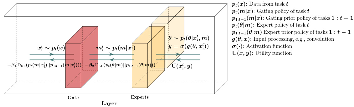
Figure 1: This figure illustrates our proposed design. Each layer implements a top $k$ expert selection conditioned on the output of the previous layer. Each expert $m$ maintains a distribution over its weights $p(\theta|m)=\mathcal N(\mu_{m},\sigma_{m})$ and a set of bias variables $b_{m}$ .

图 1: 该图展示了我们提出的设计方案。每一层根据前一层输出实现 top $k$ 专家选择机制。每个专家 $m$ 维护其权重分布 $p(\theta|m)=\mathcal N(\mu_{m},\sigma_{m})$ 和一组偏置变量 $b_{m}$。

To extend VCL to the hierarchical case, we assume that samples are drawn from a set of $M$ independent data generating processes, i.e., the likelihood is given by a mixture model $p(y|x)=$ $\begin{array}{r}{\sum_{m=1}^{M}p(m|x)p(y|m,x)}\end{array}$ . We define an indicator variable $z\in Z$ , where $z_{m}^{i,t}$ is 1 if the output $y_{i}^{t}$ of sample $i$ from task $t$ was generated by expert $m$ and zero otherwise:

为了将VCL扩展到分层情况，我们假设样本是从一组$M$个独立的数据生成过程中抽取的，即似然由混合模型$p(y|x)=$$\begin{array}{r}{\sum_{m=1}^{M}p(m|x)p(y|m,x)}\end{array}$给出。我们定义一个指示变量$z\in Z$，其中$z_{m}^{i,t}$为1表示任务$t$中样本$i$的输出$y_{i}^{t}$由专家$m$生成，否则为0：

$$
p(y_{t}^{i}|x_{t}^{i},\Theta)=\sum_{m=1}^{M}p(z_{t}^{i,m}|x_{t}^{i},\vartheta)p(y_{t}^{i}|x_{t}^{i},\omega_{m}),
$$

where $\vartheta$ are the parameters of the selection policy, $\omega_{m}$ the parameters of the $m$ -th expert, and $\Theta={\vartheta,{\omega_{m}}_{m=1}^{M^{^{.}}}}$ the combined model parameters. The posterior after observing $T$ tasks is then given by

其中 $\vartheta$ 是选择策略的参数，$\omega_{m}$ 是第 $m$ 个专家的参数，$\Theta={\vartheta,{\omega_{m}}_{m=1}^{M^{^{.}}}}$ 为组合模型参数。观察到 $T$ 个任务后的后验概率由下式给出：

$$
\begin{array}{c}{{p(\Theta|\mathcal{D}{1:T})\propto p(\vartheta)p(\omega)\displaystyle\prod_{t=1}^{T}\displaystyle\prod_{i=1}^{N_{t}}\sum_{m=1}^{M}p(z_{t}^{i,m}|x_{t}^{i},\vartheta)p(y_{t}^{i}|x_{t}^{i},\omega_{m})}}\ {{=p(\Theta)\displaystyle\prod_{t=1}^{T}p(\mathcal{D}{t}|\Theta)\propto p(\Theta|\mathcal{D}{1:T-1})p(\mathcal{D}_{T}|\Theta).}}\end{array}
$$

The Bayes posterior of an expert $p\big(\omega_{m}\vert\mathcal{D}{1:T}\big)$ is recovered by computing the marginal over the selection variables $Z$ . Again, this forms a recursion, in which the posterior $p(\Theta|\mathcal{D}{1:T})$ depends on the posterior after seeing $T-1$ tasks and the likelihood $p(\mathcal{D}_{T}|\Theta)$ . Finally, we formulate the HVCL objective for task $t$ as:

专家贝叶斯后验 $p\big(\omega_{m}\vert\mathcal{D}{1:T}\big)$ 通过计算选择变量 $Z$ 的边缘分布得到。这同样构成一个递归过程，其中后验 $p(\Theta|\mathcal{D}{1:T})$ 取决于处理完 $T-1$ 个任务后的后验以及似然函数 $p(\mathcal{D}_{T}|\Theta)$。最终，我们将任务 $t$ 的HVCL目标函数定义为：

$$
\mathcal{L}{\mathrm{HVCL}}^{t}=\sum_{i=1}^{N_{t}}\mathbb{E}{p(\Theta)}\left[\log p(y_{t}^{i}|x_{t}^{i},\Theta)\right]-\mathrm{D}{\mathrm{KL}}\left[p_{t}(\vartheta)||p_{1:t-1}(\vartheta)\right]-\mathrm{D}{\mathrm{KL}}\left[p_{t}(\omega)||p_{1:t-1}(\omega)\right],
$$

where $N_{t}$ is the number of samples in task $t$ , and the likelihood $p(\boldsymbol{y},\boldsymbol{x}|\Theta)$ is defined as in equation 3.

其中 $N_{t}$ 是任务 $t$ 中的样本数量，似然 $p(\boldsymbol{y},\boldsymbol{x}|\Theta)$ 的定义如公式3所示。

2.1 SPARSELY GATED MIXTURE-OF-VARIATION AL LAYERS

2.1 稀疏门控混合变分层

As we aim to tackle not only supervised learning problems, but also reinforcement learning problems, we assume in the following a generic scalar utility function ${\bf U}(x,f_{\boldsymbol{\theta}}(x))$ that depends both on the input $x$ and the parameterized agent function $f_{\boldsymbol{\theta}}(\boldsymbol{x})$ that generates the agent’s output $y$ . We assume the agents output function $f_{\boldsymbol{\theta}}(\boldsymbol{x})$ is composed of multiple layers. Our layer design builds on the sparsely gated Mixture-of-Expert (MoE) layers (Shazeer et al., 2017), which in turn draws on the paradigm introduced by Jacobs et al. (1991). MoEs consist of a set of $m$ experts $M$ and a gating network $\bar{p(\boldsymbol{m}\vert x)}$ whose output is a (sparse) $m$ -dimensional vector. All experts have an identical architecture but separate parameters. Let $p(m|x)$ be the gating output and $p(\boldsymbol{y}|m,x)$ the response of an expert $m$ given input $x$ . The layer’s output is then given by a weighted sum of the experts responses. To save computation time we employ a top $k$ gating scheme, where only the $k$ experts with highest gating activation are evaluated and use an additional penalty that encourages gating sparsity (see Section 2.1). In all our experiments we set $k=1$ , to drive expert specialization (see Section 2.2.1) and reduce computation time. We implement the learning objective for task $t$ as layer-wise regular iz ation in the following way:

由于我们的目标不仅是解决监督学习问题，还包括强化学习问题，因此在下文中我们假设存在一个通用的标量效用函数 ${\bf U}(x,f_{\boldsymbol{\theta}}(x))$ ，该函数同时依赖于输入 $x$ 和生成智能体输出 $y$ 的参数化智能体函数 $f_{\boldsymbol{\theta}}(\boldsymbol{x})$ 。我们假设智能体的输出函数 $f_{\boldsymbol{\theta}}(\boldsymbol{x})$ 由多个层组成。我们的层设计基于稀疏门控的混合专家 (MoE) 层 (Shazeer et al., 2017)，后者又借鉴了 Jacobs et al. (1991) 提出的范式。MoE 由一组 $m$ 个专家 $M$ 和一个门控网络 $\bar{p(\boldsymbol{m}\vert x)}$ 组成，其输出是一个（稀疏的）$m$ 维向量。所有专家具有相同的架构但参数独立。设 $p(m|x)$ 为门控输出，$p(\boldsymbol{y}|m,x)$ 为给定输入 $x$ 时专家 $m$ 的响应。该层的输出由专家响应的加权和给出。为了节省计算时间，我们采用 top $k$ 门控方案，其中仅评估门控激活最高的 $k$ 个专家，并使用额外的惩罚项来促进门控稀疏性（参见第 2.1 节）。在所有实验中，我们设置 $k=1$ 以推动专家专业化（参见第 2.2.1 节）并减少计算时间。我们将任务 $t$ 的学习目标实现为分层正则化，具体方式如下：

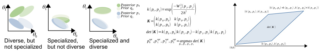
Figure 2: Left: We seek experts that are both specialized, i.e., their posterior $p$ is close to their prior $q$ , and diverse, i.e., posteriors are sufficiently distant from one another. Right: To this effect, we maximize the determinant of the kernel matrix $K$ , effectively filling the feature space. In the case of two experts this would mean to maximize $d e t(\mathbf{K})=1\stackrel{\cdot}{-}k(p_{0},\stackrel{\cdot}{p}_{1})$ , which we can achieve by maximizing the Wasser stein-2 distance between the posteriors.

图 2: 左图: 我们寻找既专业化 (即其后验 $p$ 接近其先验 $q$) 又多样化 (即后验之间保持足够距离) 的专家。右图: 为此我们最大化核矩阵 $K$ 的行列式, 从而有效填充特征空间。对于两个专家的情况, 这意味着最大化 $det(\mathbf{K})=1\stackrel{\cdot}{-}k(p_{0},\stackrel{\cdot}{p}_{1})$, 这可以通过最大化后验之间的 Wasserstein-2 距离来实现。

where $L$ is the total number of layers, $\Theta={\theta,{\vartheta_{m}}{m=1}^{M}}$ the combined parameters,and the temperature parameters $\beta_{1,2}$ govern the layer-wise trade-off between utility and information-cost.

其中 $L$ 是总层数，$\Theta={\theta,{\vartheta_{m}}{m=1}^{M}}$ 为组合参数，温度参数 $\beta_{1,2}$ 控制各层效用与信息成本之间的权衡。

Thus, we allow for two major generalizations compared to equation 5: in lieu of the log-likelihood we allow for generic utility functions, and instead of applying the constraint on the gating parameters, we apply it directly on the gating output distribution $p(m|x)$ . This implies, that the weights of the gating policy are not sampled. Otherwise the gating mechanism would involve two stochastic steps: one in sampling the weights and a second one in sampling the expert index. This potentially high selection variance hinders expert specialization (see Section 2.2.1). Encouraging the gating policy to stay close to its prior also ensures that similar inputs are assigned to the same expert. Next we consider how we could extend objective 6 further by additional terms that encourage diversity between different experts.

因此，相比公式5我们实现了两大泛化：允许使用通用效用函数替代对数似然函数，并将约束直接作用于门控输出分布$p(m|x)$而非门控参数。这意味着门控策略的权重无需采样，否则门控机制将涉及双重随机步骤——权重采样和专家索引采样。这种潜在的高选择方差会阻碍专家专业化（参见第2.2.1节）。通过促使门控策略接近其先验分布，还能确保相似输入被分配给同一专家。接下来我们将探讨如何通过引入促进专家间多样性的附加项来进一步扩展目标函数6。

2.2 ENCOURAGING EXPERT DIVERSITY

2.2 鼓励专家多样性

In the following, we argue that a diverse set of experts may mitigate catastrophic forgetting in continual learning, as experts specialize more easily in different tasks, which improves expert selection. We present two expert diversity objectives. The first one arises directly from the main learning objective and is designed to act as a regularize r on the gating policy while the second one is a more sophisticated approach that aims for diversity in the expert parameter space. The latter formulation introduces a new class of diversity measures, as we discuss in more detail in Section 4.

我们认为，多样化的专家组合可以缓解持续学习中的灾难性遗忘问题，因为专家更容易专注于不同任务，从而优化专家选择机制。我们提出两种专家多样性目标：第一种直接源自主要学习目标，旨在对门控策略进行正则化；第二种是更复杂的方案，追求专家参数空间的多样性。如第4节所述，后一种方案开创了新型多样性度量方法。

2.2.1 DIVERSITY THROUGH SPECIALIZATION

2.2.1 通过专业化实现多样性

The relationship between objectives of the form described by equation 6 with the emergence of expert specialization has been previously investigated for simple learning problems (Genewein et al., 2015) and in the context of meta-learning (Hihn & Braun, 2020b), but not in the context of continual learning. We assume a two-level hierarchical system of specialized decision-makers where lowlevel decision-makers $p(m|x)$ select which high-level decision-maker $p(\boldsymbol{y}|m,x)$ serve as experts for a particular input $x$ . By co-optimizing

方程6所描述形式的目标与专家专业化涌现之间的关系，此前已在简单学习问题 (Genewein et al., 2015) 和元学习 (Hihn & Braun, 2020b) 背景下进行过研究，但尚未在持续学习背景下探讨。我们假设一个双层专业化决策者层级系统，其中底层决策者 $p(m|x)$ 选择由哪些高层决策者 $p(\boldsymbol{y}|m,x)$ 作为特定输入 $x$ 的专家。通过协同优化

$$
\operatorname*{max}{p(y|x,m),p(m|x)}\mathbb{E}[\mathbf{U}(x,y)]-\beta_{1}I(X;M)-\beta_{2}I(X;Y|M),
$$

the combined system finds an optimal partitioning of the input space $X$ , where $I(\cdot|\cdot)$ denotes the (conditional) mutual information between random variables. In fact, the hierarchical VCL objective given by equation 5 can be regarded as a special case of the information-theoretic objective given by equation 7, if we interpret the prior as the learning strategy of task $t-1$ and the posterior as the strategy of task $t$ , and set $\beta=1$ . All these hierarchical decision systems correspond to a multi prior setting, where different priors associated with different experts can specialize on different sub-regions of the input space. In contrast, specialization in the context of continual learning can be regarded as the ability of partitioning the task space, where each expert decision-maker $m$ solves a subset of old tasks $T^{m}\subseteq T_{1:t}$ . In both cases, expert diversity is a natural consequence of specialization if the gating policy $p(m|x)$ partitions between the experts.

组合系统找到输入空间 $X$ 的最优划分，其中 $I(\cdot|\cdot)$ 表示随机变量之间的(条件)互信息。实际上，若将先验解释为任务 $t-1$ 的学习策略、后验解释为任务 $t$ 的策略，并设 $\beta=1$ ，则公式5给出的分层VCL目标可视为公式7给出的信息论目标的特例。所有这些分层决策系统都对应多先验设置，其中与不同专家关联的不同先验可专注于输入空间的不同子区域。相比之下，持续学习背景下的专业化可视为划分任务空间的能力，每个专家决策者 $m$ 解决旧任务子集 $T^{m}\subseteq T_{1:t}$ 。在这两种情况下，若门控策略 $p(m|x)$ 在专家间进行划分，则专家多样性是专业化的自然结果。

In addition to the implicit pressures for specialization already implied by equation 6, here we investigate the effect of an additional entropy cost. Inspired by recent entropy regular iz ation techniques (Eysenbach et al., 2018; Galashov et al., 2019; Grau-Moya et al., 2019), we aim to improve the gating policy by introducing the entropy cost

除了公式6中已隐含的专业化隐性压力外，我们在此研究了额外熵成本的影响。受近期熵正则化技术 (Eysenbach et al., 2018; Galashov et al., 2019; Grau-Moya et al., 2019) 的启发，我们旨在通过引入熵成本来改进门控策略

$$
{\frac{\beta_{3}}{N_{b}}}\sum_{x\in B}H(M|X)-H(M),
$$

where $M$ is the set of experts and $X$ the inputs in a mini-batch $\boldsymbol{\mathcal{B}}$ of size $N_{b}$ , and $\beta_{3}$ a weight. By maximizing the conditional entropy $H(M|X)$ we encourage high certainty in the expert gating and by minimizing the marginal entropy $H(M)$ we prefer solutions that minimize the number of active experts. We compute these values batch-wise, as the full entropies over $p(x)$ are not tractable.

其中 $M$ 是专家集合，$X$ 是大小为 $N_{b}$ 的小批量 $\boldsymbol{\mathcal{B}}$ 中的输入，$\beta_{3}$ 为权重。通过最大化条件熵 $H(M|X)$ 来鼓励专家门控的高确定性，同时通过最小化边际熵 $H(M)$ 来偏好激活专家数量最少的解。由于 $p(x)$ 上的完整熵难以计算，我们按批次计算这些值。

2.2.2 PARAMETER DIVERSITY

2.2.2 参数多样性

Our second diversity formulation builds on Determinant al Point Processes (DPPs) (Kulesza et al., 2012), a mechanism that produces diverse subsets by sampling proportionally to the determinant of the kernel matrix of points within the subset (Macchi, 1975). A point process $P$ on a ground set $Y$ is a probability measure over finite subsets of $Y$ . $P$ is a DPP if, when $Y$ is a random subset drawn according to $P$ , we have, for every $A\subset Y$ , $P(A\subset Y)=d e t(K_{A})$ for some real, symmetric $N\times N$ matrix $K$ indexed by the elements of $Y$ . Here, $K_{A}=[K_{i j}]{i,j\in A}$ denotes the restriction of $K$ to the entries indexed by elements of $A$ , and we adopt $d e t(K_{\emptyset})\overline{{=}}1$ . If $A={i}$ is a singleton, then we have $P(i\in Y)=K_{i,i}$ . In this case, the diagonal of $K$ gives the marginal probabilities of inclusion for individual elements of $Y$ . Since $P$ is a probability measure, all principal minors of $K$ must be non negative, and thus $K$ itself must be positive semi definite, which we can achieve by constructing $K$ by a kernel function $k(x_{0},x_{1})$ , such that for any $x_{0},x_{1}\in\mathcal{X}$ :

我们的第二种多样性公式基于行列式点过程 (Determinantal Point Processes, DPPs) [20]，该机制通过根据子集内点的核矩阵行列式比例采样来生成多样化子集 [21]。在基础集 $Y$ 上的点过程 $P$ 是 $Y$ 的有限子集上的概率测度。若当 $Y$ 是根据 $P$ 抽取的随机子集时，对于任意 $A\subset Y$ 满足 $P(A\subset Y)=det(K_{A})$，则称 $P$ 为 DPP，其中 $K$ 是由 $Y$ 的元素索引的实对称 $N\times N$ 矩阵。此处 $K_{A}=[K_{ij}]{i,j\in A}$ 表示 $K$ 限制在由 $A$ 的元素索引的条目，我们约定 $det(K_{\emptyset})\equiv1$。若 $A={i}$ 为单例集，则有 $P(i\in Y)=K_{i,i}$。此时，$K$ 的对角线给出了 $Y$ 中单个元素被包含的边际概率。由于 $P$ 是概率测度，$K$ 的所有主子式必须非负，因此 $K$ 本身必须是半正定的。这可以通过核函数 $k(x_{0},x_{1})$ 构造 $K$ 来实现，使得对于任意 $x_{0},x_{1}\in\mathcal{X}$：

$$
k(\boldsymbol{x}{0},\boldsymbol{x}{1})=\langle\phi(\boldsymbol{x}{0}),\phi(\boldsymbol{x}{1})\rangle_{\mathcal{F}},
$$

where $\mathcal{X}$ is a vector space and $\mathcal{F}$ is a inner-product space such that $\forall x\in\mathcal{X}:\phi(x)\in\mathcal{F}$ . Specifically, we use a exponential kernel based on the Wasser stein-2 distance $W(p,q)$ between two probability distributions $p$ and $q$ . The $p^{\mathrm{th}}$ Wasser stein distance between two probability measures $p$ and $q$ in $P_{p}(M)$ is defined as

其中 $\mathcal{X}$ 是一个向量空间，$\mathcal{F}$ 是一个内积空间，满足 $\forall x\in\mathcal{X}:\phi(x)\in\mathcal{F}$。具体而言，我们使用基于两个概率分布 $p$ 和 $q$ 之间 Wasserstein-2 距离 $W(p,q)$ 的指数核。两个概率测度 $p$ 和 $q$ 在 $P_{p}(M)$ 中的第 $p^{\mathrm{th}}$ Wasserstein 距离定义为

$$
W_{p}(p,q):=\left(\operatorname*{inf}{\gamma\in\Gamma(p,q)}\int_{M\times M}d(x,y)^{p}\mathrm{d}\gamma(x,y)\right)^{1/p},
$$

where $\Gamma(p,q)$ denotes the collection of all measures on $M\times M$ with marginals $p$ and $q$ on the first and second factors. Let $p$ and $q$ be two isotropic Gaussian distributions and $W_{2}^{2}(q,p)$ the Wasser stein-2 distance between $p$ and $q$ . The exponential Wasser stein-2 kernel is then defined by

其中 $\Gamma(p,q)$ 表示在 $M\times M$ 上所有具有边缘分布 $p$ 和 $q$ 的测度集合。设 $p$ 和 $q$ 为两个各向同性高斯分布，$W_{2}^{2}(q,p)$ 为 $p$ 和 $q$ 之间的 Wasserstein-2 距离。则指数 Wasserstein-2 核定义为

$$
k(p,q)=\exp\left(-\frac{W_{2}^{2}(p,q)}{2h^{2}}\right),
$$

where $\mu_{p,q}$ are the means and $d_{p,q}$ the diagonal entries of distributions $p$ and $q$ . We provide a more detailed derivation of equation 12 in Appendix A. From a geometric perspective, the determinant of

其中 $\mu_{p,q}$ 是均值，$d_{p,q}$ 是分布 $p$ 和 $q$ 的对角线元素。我们在附录A中提供了方程12的更详细推导。从几何角度来看，行列式的

基准方法	S-MNIST	P-MNIST	基准方法	Split-CIFAR-10	CIFAR-100
密集神经网络	86.15 (±1.00)	17.26 (±0.19)	卷积神经网络	66.62 (±1.06)	19.80 (±0.19)
离线重训练+任务先知	99.64 (±0.03)	97.59 (±0.02)	离线重训练+任务先知	80.42 (±0.95)	52.30 (±0.02)
单头与任务无关			单头与任务无关
VCL (ours)	97.50 (±0.33)	97.07 (±0.62)	HVCL (ours)	78.41 (±1.18)	33.10 (±0.62)
VCL w/GR (ours)	98.60 (±0.35)	97.47 (±0.52)	HVCL w/GR (ours)	81.00 (±1.15)	37.20 (±0.52)
GCL w/BNN [20]	97.70 (±0.03)	92.50 (±0.01)	CL-DR [21]	86.72 (±0.30)	25.62 (±0.22)
脑启发的RtF [22]	99.66 (±0.13)	97.31 (±0.04)	NCL [23]		38.79 (±0.24)
IBNN [24]	91.00 (±2.20)	93.70 (±0.60)	TLR [25]	74.89 (±0.61)
CL [26]	98.71 (±0.06)	97.51 (±0.05)	MAS [27]	73.50 (±1.54)
LR [25]	80.64 (±1.25)		多头与任务感知
多头与任务感知
GR+蒸馏 [28]	99.59 (±0.40)	97.51 (±0.04)	GEM [29]	82.90 (±1.20)	79.10 (±1.60)
CL [30]	98.50 (±1.78)	96.60 (±1.34)	CCL wFP [31]	86.33 (±1.47)	65.19 (±0.65)
URL [32]	99.10 (±0.06)		HAL [33]	75.19 (±2.57)	47.88 (±2.76)
AML [34]	97.95 (±0.07)		SI [35]	63.31 (±3.79)	36.33 (±4.23)
EN [36]	99.26 (±0.01)		AGEM [37]	74.07 (±0.76)	46.88 (±1.81)

Table 1: Results in the supervised CL benchmarks. Results were averaged over ten random seeds with the standard deviation given in the parenthesis. We report results of other methods as given in their original studies.

表 1: 监督式持续学习基准测试结果。结果取十个随机种子的平均值，括号内为标准差。其他方法的结果按其原始研究数据呈现。

the kernel matrix represents the volume of a parallel e piped spanned by feature maps corresponding to the kernel choice. We seek to maximize this volume, effectively filling the parameter space – see Figure 2 for an illustration.

核矩阵表示由与核选择对应的特征映射所张成的平行多面体的体积。我们的目标是最大化这一体积，从而有效填满参数空间——具体说明见图 2。

3 EXPERIMENTS

3 实验

We evaluate our approach in current supervised CL benchmarks in Section 3.1, in a generative learning setting in Section 3.2, and in the CRL setup in Section 3.3. We give experimental details in Appendix C.

我们在第3.1节评估当前监督式持续学习基准中的方法，在第3.2节评估生成式学习场景，在第3.3节评估持续强化学习(CRL)配置。实验细节详见附录C。

3.1 CONTINUAL SUPERVISED LEARNING SCENARIOS

3.1 持续监督学习场景

The basic setting of continual learning is defined as an agent which sequentially observes data from a series of tasks while maintaining performance on older tasks. We evaluate the performance of our method in this setting in split MNIST, permuted MNIST, split CIFAR-10/100 (see Table 1). We follow the domain incremental setup (van de Ven et al., 2020), where task information is not available, but we also compare against task-incremental methods, where the task information is available, to give a complete overview of current methods.

持续学习的基本设定被定义为一个智能体 (agent) ，它按顺序观察来自一系列任务的数据，同时保持对旧任务的性能。我们在 split MNIST、permuted MNIST、split CIFAR-10/100 (见表 1) 等场景中评估了本方法的性能。我们遵循域增量设置 (van de Ven et al., 2020) ，其中任务信息不可用，但为了全面概述现有方法，我们也与任务信息可用的任务增量方法进行了对比。

The first benchmark builds on the MNIST dataset. Five binary classification tasks from the MNIST dataset arrive in sequence and at time step $t$ the performance is measured as the average classification accuracy on all tasks up to task $t$ . In permuted MNIST the task received at each time step $t$ consists of labeled MNIST images whose pixels have undergone a fixed random permutation. The second benchmark is a variation of the CIFAR-10/100 datasets. In Split CIFAR-10, we divide the ten classes into five binary classification tasks. CIFAR-100 is like the CIFAR-10, except it has 100 classes and tasks are defined as a 10-way classification problem, thus forming ten tasks in total.

首个基准测试基于MNIST数据集。该实验按顺序处理MNIST数据集中的五个二元分类任务，在时间步$t$时，性能指标被量化为前$t$个任务的平均分类准确率。在置换MNIST任务中，每个时间步$t$接收的任务由经过固定随机像素置换的带标签MNIST图像组成。第二个基准测试是CIFAR-10/100数据集的变体：在分割CIFAR-10中，我们将十种类别划分为五个二元分类任务；而CIFAR-100除包含100个类别外与CIFAR-10类似，其任务被定义为十路分类问题，共形成十个任务。

We achieve comparable results to current state-of-the-art approaches (see Table 1) on all supervised learning benchmarks.

我们在所有监督学习基准测试中取得了与当前最先进方法 (参见表 1) 相当的结果。

3.2 GENERATIVE CONTINUAL LEARNING

3.2 生成式持续学习

Generative CL is a simple but powerful paradigm (van de Ven et al., 2020). The main idea is to learn the data generating distribution and simulate data of previous tasks. We can extend our approach to the generative setting by modeling a variation al auto encoder using the novel layers we propose in this work.

生成式持续学习 (Generative CL) 是一种简单而强大的范式 [20]。其核心思想是学习数据生成分布并模拟先前任务的数据。通过使用本文提出的新型层对变分自编码器 (variational auto encoder) 进行建模，我们可以将该方法扩展到生成式场景。

We model the distribution of the latent variable $z$ in the variation al auto encoder by using a densely connected MoVE layer with 3 experts. Using multiple experts enables us to capture a richer class of distributions than a single Gaussian distribution could, as is usually the case in simple VAEs.

我们通过使用具有3个专家的密集连接MoVE层来建模变分自编码器中潜变量$z$的分布。与简单VAE中通常使用的单一高斯分布相比，采用多个专家使我们能够捕捉更丰富的分布类别。

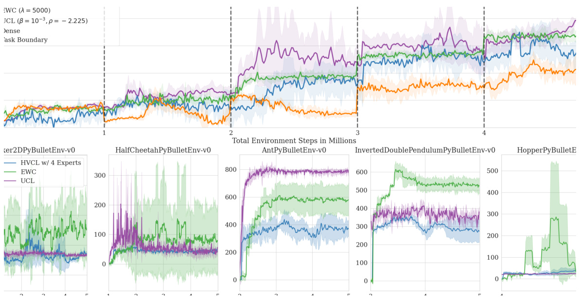
Figure 3: In this figure we show results in the CRL benchmark. To measure the continual learning performance in the RL settings, we normalize rewards and plot the sum of normalized rewards. The maximum of 5.0 indicates no forgetting, while 1.0 shows the total forgetting of old tasks. We comapre against EWC (Kirkpatrick et al., 2017), and UCL (Ahn et al., 2019).

图 3: 本图展示了CRL基准测试中的结果。为了衡量强化学习环境下的持续学习性能，我们对奖励进行归一化处理并绘制归一化奖励的总和。最大值5.0表示没有遗忘，而1.0则表示对旧任务的完全遗忘。我们与EWC (Kirkpatrick et al., 2017) 和UCL (Ahn et al., 2019) 进行了对比。

We can interpret this as $z$ following a Gaussian Mixture Model, whose components are mutually exclusive and modeled by experts. We integrate the generated data by optimizing a mixture of the loss on the new task data and the loss of the generated data We were able to improve our results in the supervised settings by incorporating a generative component, as we show in Table 1. We show additional empirical results in Appendix D.1.

我们可以将其解释为 $z$ 服从高斯混合模型 (Gaussian Mixture Model)，其分量相互排斥并由专家建模。我们通过优化新任务数据损失和生成数据损失的混合来整合生成的数据。如表 1 所示，通过加入生成式组件，我们在监督学习场景中提升了结果。更多实证结果见附录 D.1。

3.3 CONTINUAL REINFORCEMENT LEARNING

3.3 持续强化学习

In the continual reinforcement learning (CRL) setting, the agent is tasked with finding an optimal policy in sequentially arriving RL problems. To benchmark our method, we follow the experimental protocol of Ahn et al. (2019) and use a series of tasks from the PyBullet environments (Ellen berger, 2018–2019). The environments we selected have different states and action dimensions. This implies we can’t use a single model to learn policies and value functions. To remedy this, we pad each state and action with zeros to have equal dimensions. The Ant environment has the highest dimensionality with a state dimensionality of 28 and an action dimensionality of 8. All others are zero-padded to have this dimensionality.

在持续强化学习 (CRL) 设定中，智能体的任务是在连续到达的强化学习问题中寻找最优策略。为了对我们的方法进行基准测试，我们遵循 Ahn 等人 (2019) 的实验方案，并使用来自 PyBullet 环境 (Ellen berger, 2018–2019) 的一系列任务。我们选择的环境具有不同的状态和动作维度。这意味着我们无法使用单一模型来学习策略和价值函数。为了解决这个问题，我们用零填充每个状态和动作以使维度相等。Ant 环境具有最高的维度，其状态维度为 28，动作维度为 8。所有其他环境都通过零填充以达到该维度。

Here, we extend SAC (Haarnoja et al., 2018) by implementing all neural networks with MovE layers. When a new task arrives, the old posterior over the expert parameters and the gating posterior become the new priors. After each update step in task $t$ , we evaluate the agent in all previous tasks $T_{1:t}$ for three episodes each. We divide the reward achieved during evaluation by the mean reward during training and report the cumulative normalized reward, which gives an upper bound of $t$ in the $t$ -th task.

在这里，我们通过使用MovE层实现所有神经网络来扩展SAC (Haarnoja等人，2018)。当新任务到达时，专家参数的旧后验和门控后验成为新的先验。在任务$t$的每次更新步骤后，我们评估智能体在所有先前任务$T_{1:t}$中的表现，每个任务进行三次测试。我们将评估期间获得的奖励除以训练期间的平均奖励，并报告累积归一化奖励，这在第$t$个任务中给出了$t$的上限。

We compare our approach against a simple continuously trained SAC implementation with dense neural networks, EWC (Kirkpatrick et al., 2017), and the recently published UCL (Ahn et al., 2019) method. UCL is similar to our approach in that it also employs Bayesian neural networks, but the weight regular iz ation acts on a per-weight basis. Note that UCL and EWC both require task information to compute task-specific losses. Our results (see Figure 3) show that our approach can sequentially learn new policies while maintaining an acceptable performance on previously seen tasks. Our method outperforms UCL (Ahn et al., 2019) and EWC (Kirkpatrick et al., 2017). In this setting naively training the agent sequentially (labeled ”Dense”) yields poor performance. This behavior indicates the complete forgetting of old policies.

我们将我们的方法与以下方法进行比较：使用密集神经网络的简单持续训练SAC实现、EWC (Kirkpatrick等人，2017) 以及最近发表的UCL (Ahn等人，2019) 方法。UCL与我们的方法类似，也采用了贝叶斯神经网络，但其权重正则化是基于单个权重进行的。需要注意的是，UCL和EWC都需要任务信息来计算特定任务的损失。我们的结果（见图3）表明，我们的方法可以顺序学习新策略，同时在先前见过的任务上保持可接受的性能。我们的方法优于UCL (Ahn等人，2019) 和EWC (Kirkpatrick等人，2017)。在这种设置下，简单地顺序训练智能体（标记为"Dense"）表现较差。这种行为表明旧策略被完全遗忘。

4 DISCUSSION

4 讨论

The principle we propose in this work falls into a wider class of methods that deal with learning and decision-making problems by integrating information-theoretic cost functions. Such informationconstrained machine learning methods have enjoyed recent interest in a variety of research fields, e.g., as reinforcement learning (Eysenbach et al., 2018; Ghosh et al., 2018; Leibfried & Grau-Moya, 2019; Hihn et al., 2019; Arumugam et al., 2020), MCMC optimization (Hihn et al., 2018; Pang et al., 2020), meta-learning (Rothfuss et al., 2018; Hihn & Braun, 2020a), continual learning (Nguyen et al., 2017; Ahn et al., 2019), and self-supervised learning (Thiam et al., 2021; Tsai et al., 2021).

我们在本工作中提出的原则属于一类更广泛的方法，这些方法通过整合信息论成本函数来处理学习和决策问题。这类信息约束的机器学习方法最近在多个研究领域受到关注，例如强化学习 (Eysenbach et al., 2018; Ghosh et al., 2018; Leibfried & Grau-Moya, 2019; Hihn et al., 2019; Arumugam et al., 2020)、MCMC优化 (Hihn et al., 2018; Pang et al., 2020)、元学习 (Rothfuss et al., 2018; Hihn & Braun, 2020a)、持续学习 (Nguyen et al., 2017; Ahn et al., 2019) 以及自监督学习 (Thiam et al., 2021; Tsai et al., 2021)。

Currently, there are only few methods that perform well in supervised CL and in CRL (e.g., Ahn et al., 2019; Jung et al., 2020; Cha et al., 2020). These methods require task information, as they either keep a set of separate task-specific heads (Ahn et al., 2019; Jung et al., 2020) or compute task-specific losses (Cha et al., 2020). This makes our method one of the first task-agnostic CL approaches to do so.

目前，仅有少数方法在监督式持续学习(CL)和类别增量学习(CRL)中表现良好 (例如 Ahn et al., 2019; Jung et al., 2020; Cha et al., 2020)。这些方法需要任务信息，因为它们要么维护一组独立的任务特定头部 (Ahn et al., 2019; Jung et al., 2020)，要么计算任务特定损失 (Cha et al., 2020)。这使得我们的方法成为首批实现任务无关的持续学习方案之一。

The hierarchical structure we employ is a variant of the Mixture-of-Experts (MoE) model (Jacobs et al., 1991), specifically an extension of the sparsely-gated MoE layers (Shazeer et al., 2017). Sparsely-gated MoE layers enforce a balanced load between experts. In our work, we removed the incentive to equally distribute inputs, as we aim to find specialized experts, which contradicts a balanced load. The computational advantage remains, as we still activate only the top-1 expert.

我们采用的层级结构是混合专家模型 (Mixture-of-Experts, MoE) (Jacobs et al., 1991) 的一个变体，具体来说是稀疏门控 MoE 层 (Shazeer et al., 2017) 的扩展。稀疏门控 MoE 层强制专家间负载均衡。在我们的工作中，我们移除了均衡分配输入的约束机制，因为我们的目标是寻找专业化专家，这与负载均衡的目标相矛盾。计算优势仍然存在，因为我们仅激活 top-1 专家。

Our method is similar to the approach described by Hihn & Braun (2020b) but differs in two key aspects. Firstly, we provide a more stable learning procedure as our layers can readily offer endto-end training. Secondly, we implement the information-processing constraints on the parameters instead of the output of the experts, thus shifting the information cost from decision-making to learning.

我们的方法与Hihn & Braun (2020b)描述的方法类似，但在两个关键方面有所不同。首先，我们提供了更稳定的学习过程，因为我们的层可以轻松实现端到端训练。其次，我们在参数而非专家输出上实施信息处理约束，从而将信息成本从决策转移到学习上。

Several methods in the current CL literature rest on modular architectures (e.g., Fernando et al., 2017; Collier et al., 2020; Lin et al., 2019; Lee et al., 2020). Lin et al. (2019) propose to condition model parameters on the inputs by learning a (deterministic) grouping function. Our approach differs in two main ways. First, our method can capture uncertainty allowing us to learn stochastic tasks. Second, our design can incorporate up to $2^{n}$ paths (or groupings) through a neural net with $n$ layers, making it more flexible than learning a mapping function. Lee et al. (2020) propose a MoE model for continual learning, in which the number of experts increases dynamically, utilizing DirichletProcess-Mixtures (Antoniak, 1974) to infer the number of experts. The authors argue that since the gating mechanism is itself a classifier, training it in an online fashion would result in catastrophic forgetting. To remedy this, they implement a generative model per expert $m$ to model $p(m|x)$ and approximate the output as $\begin{array}{r}{p(y|x)\stackrel{{}}{\approx}\sum_{m}p(y|x)p(m|x)}\end{array}$ . In our work, we have demonstrated that it is possible to implement a gating mechanism based only on the input by coupling it with an information-theoretic objective to prevent catastrophic forgetting.

当前持续学习(CL)文献中的几种方法依赖于模块化架构(如 Fernando et al., 2017; Collier et al., 2020; Lin et al., 2019; Lee et al., 2020)。Lin等人(2019)提出通过学习一个(确定性)分组函数，使模型参数基于输入进行条件化。我们的方法在两个方面有所不同。首先，我们的方法能够捕捉不确定性，从而可以学习随机任务。其次，我们的设计可以在具有$n$层的神经网络中整合多达$2^{n}$条路径(或分组)，这比学习映射函数更具灵活性。Lee等人(2020)提出了一种用于持续学习的混合专家(MoE)模型，其中专家数量动态增长，利用狄利克雷过程混合(Antoniak, 1974)来推断专家数量。作者认为，由于门控机制本身就是一个分类器，以在线方式训练会导致灾难性遗忘。为解决这个问题，他们为每个专家$m$实现了一个生成模型来建模$p(m|x)$，并将输出近似为$\begin{array}{r}{p(y|x)\stackrel{{}}{\approx}\sum_{m}p(y|x)p(m|x)}\end{array}$。在我们的工作中，我们证明了仅基于输入实现门控机制是可行的，并通过将其与信息论目标相结合来防止灾难性遗忘。

Recently, several diversity measures have been proposed. Parker-Holder et al. (2020) introduce a DDP-based method based on the different states a given policy may reach. Dai et al. (2021) propose to augment the sampling process in hindsight experience replay (An dry ch owicz et al., 2017) with a DPP-diversity bonus. The method we propose differs from previous methods as we define diversity in parameter space instead of the policy outcomes or inputs. Additionally, as we define it on parameters instead of actions, we can apply it straightforwardly to any problem formulation, as our experiments show.

最近，研究者们提出了多种多样性衡量方法。Parker-Holder等人 (2020) 提出了一种基于给定策略可能到达不同状态的DDP方法。Dai等人 (2021) 则建议在后见经验回放 (An dry ch owicz等人, 2017) 的采样过程中加入DPP多样性奖励。我们提出的方法与之前的方法不同，因为我们在参数空间而非策略结果或输入中定义多样性。此外，由于我们在参数而非动作上定义多样性，如实验所示，该方法可直接应用于任何问题形式。

5 CONCLUSION

5 结论

We introduced a hierarchical approach to task-agnostic continual learning, derived an application, and extensively evaluated this method in supervised CL and CRL. While we removed the taskinformation limitation, we achieved results competitive to task-aware and to task-agnostic algorithms. We argued that both VCL and hierarchical VCL have strong connections to an informationtheoretic formulation of bounded rationality. We designed a diversity objective that stabilizes learning and further reduces the risk of catastrophic forgetting. Our method builds on generic utility functions, we can apply it independently of the underlying problem, which makes our method one of the first to do so.

我们引入了一种与任务无关的层次化持续学习方法，推导了应用实例，并在监督式持续学习(CL)和持续强化学习(CRL)中对该方法进行了全面评估。在消除任务信息限制的同时，我们的方法取得了与任务感知算法及任务无关算法相当的结果。我们论证了VCL(变分持续学习)和层次化VCL都与有限理性的信息论表述存在紧密联系。通过设计多样性目标函数，我们的方法能稳定学习过程并进一步降低灾难性遗忘风险。该方法基于通用效用函数构建，可独立应用于各类底层问题，这使其成为首批实现该特性的方法之一。

ACKNOWLEDGMENT

致谢

This work was supported by the European Research Council, grant number ERC-StG-2015-ERC, Project ID: 678082, “BRISC: Bounded Rationality in Sensor i motor Coordination”.

本研究由欧洲研究理事会资助，资助编号为ERC-StG-2015-ERC，项目ID：678082，项目名称："BRISC：感觉运动协调中的有限理性"。

Dushyant Rao, Francesco Visin, Andrei Rusu, Razvan Pascanu, Yee Whye Teh, and Raia Hadsell. Continual unsupervised representation learning. Advances in Neural Information Processing Systems, 32, 2019.

Dushyant Rao、Francesco Visin、Andrei Rusu、Razvan Pascanu、Yee Whye Teh 和 Raia Hadsell。持续无监督表示学习。神经信息处理系统进展，32，2019。

A WASSER STEIN-DISTANCE BETWEEN TWO GAUSSIANS

两个高斯分布之间的Wasserstein距离

The $W_{2}^{2}$ distance between two Gaussians is given by

两个高斯分布之间的 $W_{2}^{2}$ 距离由下式给出

$$
W_{2}^{2}(p,q)=||\mu_{p}-\mu_{q}||{2}^{2}+||\sqrt{d_{p}}-\sqrt{d_{q}}||_{2},
$$

Proof: Let $p=\mathcal{N}(\mu_{p},\Sigma_{p})$ and $q=\mathcal{N}(\mu_{q},\sigma_{q})$ be two Guassian distributions. The Wasser stein-2 distance between $p$ and $q$ is then given by

证明：设 $p=\mathcal{N}(\mu_{p},\Sigma_{p})$ 和 $q=\mathcal{N}(\mu_{q},\sigma_{q})$ 为两个高斯分布。则 $p$ 与 $q$ 之间的 Wasserstein-2 距离由下式给出

$$
W_{2}^{2}(p,q)=||\mu_{p}-\mu_{q}||{2}^{2}+{\mathcal{B}}(\Sigma_{p},\Sigma_{q}),
$$

where $\boldsymbol{\mathcal{B}}$ is the Bures metric between two positive semi-definite matrices:

其中 $\boldsymbol{\mathcal{B}}$ 是两个半正定矩阵之间的Bures度量：

$$
\begin{array}{r}{\mathcal{B}(\Sigma_{p},\Sigma_{q})=t r(\Sigma_{p}+\Sigma_{q}-2(\Sigma_{p}^{1/2}\Sigma_{q}\Sigma_{p}^{1/2})^{1/2},}\end{array}
$$

where $t r(A)$ is the trace of a matrix $A$ and $A^{1/2}$ is the matrix square root. Matrix square roots are computationally expensive to compute and there can potentially be and infinite number of solutions. In the case where $p$ and $q$ are Gaussian mean-field approximations, i.e., all dimensions are independent, $\Sigma_{p}$ and $\Sigma_{q}$ are given by diagonal matrices, such that $\Sigma_{p}=\operatorname{diag}(d_{p}){i}$ and $\Sigma_{q}=\operatorname{diag}(d_{q}){i}$ . The Bures metric then reduces to the Hellinger distance between the diagonals $d_{p}$ and $d_{q}$ , and we have:

其中 $tr(A)$ 是矩阵 $A$ 的迹，$A^{1/2}$ 是矩阵平方根。矩阵平方根的计算成本很高，且可能存在无限多个解。当 $p$ 和 $q$ 为高斯平均场近似（即所有维度相互独立）时，$\Sigma_{p}$ 和 $\Sigma_{q}$ 由对角矩阵给出，即 $\Sigma_{p}=\operatorname{diag}(d_{p}){i}$ 和 $\Sigma{q}=\operatorname{diag}(d_{q}){i}$。此时 Bures 度量简化为对角线 $d_{p}$ 与 $d_{q}$ 之间的 Hellinger 距离，可得：

$$
W_{2}^{2}(p,q)=||\mu_{p}-\mu_{q}||{2}^{2}+||\sqrt{d_{p}}-\sqrt{d_{q}}||_{2}.
$$

B WASSER STEIN-2 EXPONENTIAL KERNEL

B WASSERSTEIN-2 指数核

The exponential Wasser stein-2 kernel between isotropic Gaussian distributions $p$ and $q$ with kernel width $h$ defined by

各向同性高斯分布 $p$ 和 $q$ 之间基于核宽度 $h$ 的指数Wasserstein-2核

$$
k(p,q)=\exp\left(-\frac{W_{2}^{2}(p,q)}{2h^{2}}\right)
$$

is a valid kernel function.

是一个有效的核函数。

Proof: The simplest way to show a kernel function $k$ is valid is by deriving $k$ from other valid kernels. We can express the Wasser stein distance as the sum of two norms as shown in equation 16. The euclidean norm and the Hellinger distance both form inner product spaces and are thus valid kernel functions. Their sum is also a valid kernel function, which makes the Wasser stein distance on isotropic Gaussians a valid kernel. If $k(p,q)$ is a valid kernel, then $\exp(k(p,q))$ is also a valid kernel.

证明：证明核函数 $k$ 有效的简单方法是从其他有效核推导出 $k$。如公式16所示，我们可以将Wasserstein距离表示为两个范数之和。欧几里得范数和Hellinger距离都构成内积空间，因此是有效的核函数。它们的和也是一个有效的核函数，这使得各向同性高斯分布上的Wasserstein距离成为有效核。若 $k(p,q)$ 是有效核，则 $\exp(k(p,q))$ 同样构成有效核。

C EXPERIMENT DETAILS

C 实验细节

To implement variation al layers we use Gaussian distributions. For simplicity we use a $D-$ dimensional Gaussian mean-field approximate posterior $\begin{array}{r}{q_{t}(\theta)=\prod_{d=1}^{D}\mathcal{N}(\bar{\theta}_{t}|\bar{p}_{t,d},\sigma_{t,d}^{2})}\end{array}$ . We use the flip-out estimator (Wen et al., 2018) to approximate the gradi ents. In practice, we draw a single sample to approximate the expectation.

为实现变分层，我们采用高斯分布。为简化计算，使用$D-$维高斯均值场近似后验$\begin{array}{r}{q_{t}(\theta)=\prod_{d=1}^{D}\mathcal{N}(\bar{\theta}_{t}|\bar{p}_{t,d},\sigma_{t,d}^{2})}\end{array}$。通过flip-out估计器 (Wen et al., 2018) 近似梯度计算，实际应用中仅抽取单一样本进行期望值近似。

C.1 MNIST EXPERIMENTS

C.1 MNIST 实验

For split MNIST experiments we used dense layers for both the VAE and the classifier. The VAE encoder contains two layers with 256 units each, followed by 64 units (64 units for the mean and 64 units for log-variance) for the latent variable, and two layers with 256 units for the decoder, followed by an output layer with $28*28=784$ units. This assumes isotropic Gaussians as priors and posteriors over the latent variable and allows to compute the $\mathrm{D}{\mathrm{KL}}$ if closed form. We used only one expert for the VAE with $\beta_{1}=0.002$ , $\beta_{2}=0.75$ , a diversity bonus weight of 0.01 and leaky ReLU activation s (Maas et al., 2013) in the hidden layers. We trained with a batch size 256 for 150 epochs. The VAE output activation function is a sigmoid and we trained it using a binary crossentropy loss between the normalized pixel values of the original and the reconstructed images. We used no other regular iz ation methods on the VAE. We used 10.000 generated samples after each task.

在分割MNIST实验中，我们为VAE和分类器均使用了全连接层。VAE编码器包含两个256单元的层，随后是64单元的潜变量层（均值和对数方差各64单元），解码器则包含两个256单元的层，最终输出层为$28*28=784$单元。该架构假设潜变量的先验和后验均为各向同性高斯分布，并允许在闭式解情况下计算$\mathrm{D}{\mathrm{KL}}$。我们仅使用一个专家VAE，参数设置为$\beta_{1}=0.002$、$\beta_{2}=0.75$，多样性奖励权重为0.01，隐藏层采用Leaky ReLU激活函数（Maas等人，2013）。训练批次大小为256，共进行150轮迭代。VAE输出层使用sigmoid激活函数，并通过原始图像与重建图像归一化像素值间的二元交叉熵损失进行训练。未对VAE采用其他正则化方法。每个任务完成后生成10,000个样本。

The classifier consists of two dense layers, each with 256 units with leaky ReLU activation s (Maas et al., 2013) and dropout (Srivastava et al., 2014) layers, followed by an output layer with two units. All layers of the classifier have two experts. We trained with batch size 256 for 150 epochs using Adam (Kingma & Ba, 2015) with a learning rate of $6*10^{-4}$ . In the permuted MNIST setting we used the same architecture, but increased the number of units to 512.

分类器由两个密集层组成，每层包含256个单元并采用 leaky ReLU 激活函数 (Maas et al., 2013) 和 dropout 层 (Srivastava et al., 2014)，最后接一个含两个单元的输出层。分类器的所有层都配备两个专家模块。训练时使用 batch size 为256，共150个 epochs，优化器采用 Adam (Kingma & Ba, 2015)，学习率设为 $6*10^{-4}$。在排列 MNIST 实验设定中，我们保持相同架构，但将单元数增至512。

C.2 CIFAR-10 EXPERIMENTS

C.2 CIFAR-10 实验

The VAE encoder consisted of five convolutional layers with stride 4 with two experts, each with 8, 16, 32, 64, and 128 units, followed by two dense units with two experts, each with 256 units. The latent variable has 128 dimensions, which we model by two dense layers: one with 128 units for the mean and one with 128 units for the log-variance. The dense layer modeling the mean has three experts, the layer for the log-variance one expert. We assume isotropic Gaussian distributions as priors and posteriors over the latent variable, which allows us to compute the $\mathrm{D}_{\mathrm{KL}}$ if closed form. The decoder mirrors the encoder and has two dense layers followed by 5 de-convolutional layers with stride 4 (the last layer has stride 3). All hidden layers use a leaky ReLU activation function (Maas et al., 2013). The VAE output activation function is a sigmoid and we trained it using a binary cross-entropy loss between the normalized pixel values of the original and the reconstructed images. We used no other regular iz ation methods on the VAE. We used 10.000 generated samples after each task.

VAE编码器由五个卷积层组成，每个卷积层步长为4，包含两个专家模块，各层单元数分别为8、16、32、64和128，随后接两个密集层，每个密集层也有两个专家模块，各含256个单元。潜变量维度为128，我们通过两个密集层建模：一个128单元的均值层（含三个专家模块）和一个128单元的对数方差层（含一个专家模块）。我们假设潜变量的先验和后验均为各向同性高斯分布，这使得我们可以闭式计算$\mathrm{D}_{\mathrm{KL}}$。解码器与编码器对称，包含两个密集层和五个反卷积层（步长4，末层步长3）。所有隐藏层采用Leaky ReLU激活函数（Maas等人，2013）。VAE输出层使用sigmoid激活函数，并通过原始图像与重建图像归一化像素值间的二元交叉熵损失进行训练。VAE未采用其他正则化方法。每个任务后生成10,000个样本。

The classifier architecture is similar to the encoder architecture. We used five convolutional layers, followed by two dense layers. All layers used two experts. The convolutional layers have 8, 16, 32, 64, and 128 units per experts, while the dense layers both have 256 units per layer. We used leaky ReLU as an activation function for the hidden layers and softmax for the output layer. We trained the classifier using a binary cross-entropy loss between the true and the predicted label. We trained with batch size 256 for 1000 epochs using the Adam optimizer with a learning rate of $3*10^{-4}$ .

分类器架构与编码器架构类似。我们使用了五个卷积层，后接两个全连接层。所有层均采用双专家机制。卷积层中每个专家分别包含8、16、32、64和128个单元，而全连接层每层各含256个单元。隐藏层采用Leaky ReLU作为激活函数，输出层使用softmax。训练时采用真实标签与预测标签之间的二元交叉熵损失函数，使用Adam优化器以$3*10^{-4}$的学习率进行1000轮训练，批处理大小为256。

C.3 REINFORCEMENT LEARNING EXPERIMENT DETAILS

C.3 强化学习实验细节

Each task was trained for one million time steps. We use the same network architecture as suggested by the authors UCL: two layer networks (actor and critics) with 16 units each. Each layer has four experts followed by leaky ReLU (Maas et al., 2013) activation functions. Each We set each SAC related hyper-parameter as proposed in the original publication (Haarnoja et al., 2018). For UCL (Ahn et al., 2019), we used the implementation provided by the authors for our experiments and use the hyper-parameters suggested in the publication. Note that the UCL implementation rests on a PPO (Schulman et al., 2017) backbone. Our CRL experiments do not use any form of replay (except for the replay buffer used by SAC).

每个任务都训练了一百万个时间步长。我们采用了与作者UCL建议相同的网络架构：两层网络（行动者和评论家），每层16个单元。每层包含四个专家模块，后接Leaky ReLU (Maas等人，2013)激活函数。所有SAC相关超参数均按照原始论文(Haarnoja等人，2018)的建议设置。对于UCL (Ahn等人，2019)，我们使用了作者提供的实现代码进行实验，并采用论文中推荐的超参数。需要注意的是，UCL的实现基于PPO (Schulman等人，2017)框架。我们的CRL实验未使用任何形式的经验回放（SAC自带的回放缓冲区除外）。

D ADDITIONAL EXPERIMENTS

D 补充实验

D.1 GENERATIVE CL

D.1 生成式CL

We introduce a generative approach to continual learning in Section 3.2 by implementing a Variational Auto-encoder using our proposed layer design. This addition improved classification performance and mitigated catastrophic forgetting, as evidenced by the results shown in Table 1. We train by integrating artificially generated data into the process by optimizing a mixture loss:

我们在第3.2节介绍了一种生成式持续学习方法，通过使用我们提出的层设计实现了一个变分自编码器 (Variational Auto-encoder)。如表1所示，这一改进提升了分类性能并缓解了灾难性遗忘问题。我们通过将人工生成的数据整合到训练过程中，并优化混合损失函数来进行训练:

$$
L(\theta)=\frac{1}{2|B_{t}|}\sum_{b\in B_{t}}\ell(b)+\frac{1}{2|B_{1:t}|}\sum_{b\in|B_{1:t}|}\ell(b),
$$

where $B_{t}$ is batch of data from the current task, $B_{1:t}$ a batch of generated data, and $\ell(b)$ a loss function on the batch $b$ .

其中 $B_{t}$ 是当前任务的数据批次，$B_{1:t}$ 是生成数据的批次，$\ell(b)$ 是批次 $b$ 上的损失函数。

Borrowing methods from generative learning, we investigate the performance of our proposed VAE design further, with the main focus on the quality of the generated images. We can not measure the accuracy directly, as artificial images lack labels. Thus we first use the trained classifier to obtain labels and compute metrics based on these self-generated labels. We opted for the Inception Score (IS) (Salimans et al., 2016), as it is widely used in the generative learning community. In this initially proposed formulation, the IS builds on the $\mathrm{D}_{\mathrm{KL}}$ between the conditional and the marginal class probabilities as returned by a pre-trained Inception model (Szegedy et al., 2015). To investigate the quality of the generated images concerning the continually trained classifier, we use a different version of the Inception Score, which we defined as

借鉴生成式学习的方法，我们进一步研究了所提出的VAE设计性能，重点关注生成图像的质量。由于人工生成的图像缺乏标签，我们无法直接测量准确性。因此，我们首先使用训练好的分类器获取标签，并基于这些自生成的标签计算指标。我们选择了初始分数(IS) (Salimans等人，2016)，因为它在生成式学习领域被广泛使用。在这个最初提出的公式中，IS建立在预训练Inception模型(Szegedy等人，2015)返回的条件类概率和边际类概率之间的$\mathrm{D}_{\mathrm{KL}}$上。为了研究生成图像在持续训练分类器中的质量，我们使用了不同版本的初始分数，定义为

Figure 4: Left and middle: measures for the generator quality. Right: The first two rows depict original images and the corresponding reconstructions. The following five rows are images sampled from the VAE prior after each task (automobiles vs. airplanes, birds vs. cats, deers vs. frogs, dogs vs. horses, and ships vs. trucks).

图 4: 左侧与中部: 生成器质量的评估指标。右侧: 前两行展示原始图像及对应重建结果，后续五行呈现每项任务(汽车vs飞机、鸟类vs猫类、鹿类vs蛙类、犬类vs马类、船舶vs卡车)完成后从VAE先验中采样的图像。

$$
I S_{T}(G_{1:T})=\mathbb{E}{x\sim G_{1:T}}\left[\mathrm{D}{\mathrm{KL}}\left[p_{1:T}(y|x)||p_{1:T}(y)\right]\right],
$$

where $G_{1:T}$ is the data generator trained on tasks up to $T$ , $p_{1:T}(y|x)$ the conditional class distribution returned by the classifier trained up to task $T$ , and $p_{1:T}(y)$ the marginal class distribution up to Task $T$ . Note that, $I S(G_{1:T})\leq\log_{2}\bar{N}{c}$ , where $N_{c}$ is the number of classes. We show $I S_{T}$ and the entropy of $p(y)$ in the split CIFAR-10 and split CIFAR-100 setting in Figure 4.

其中 $G_{1:T}$ 是在任务 $T$ 上训练的数据生成器，$p_{1:T}(y|x)$ 是由任务 $T$ 上训练的分类器返回的条件类别分布，$p_{1:T}(y)$ 是任务 $T$ 上的边缘类别分布。注意 $I S(G_{1:T})\leq\log_{2}\bar{N}{c}$，其中 $N_{c}$ 是类别数量。我们在图 4 中展示了分割 CIFAR-10 和分割 CIFAR-100 设置下的 $I S_{T}$ 和 $p(y)$ 的熵。

[论文翻译]变分专家混合 (MIXTURE-OF-VARIATION EXPERTS) 持续学习

原文地址：https://arxiv.org/pdf/2110.12667v4