Meta-Transfer Learning for Few-Shot Learning

基于元迁移学习的少样本学习

Abstract

摘要

Meta-learning has been proposed as a framework to address the challenging few-shot learning setting. The key idea is to leverage a large number of similar few-shot tasks in order to learn how to adapt a base-learner to a new task for which only a few labeled samples are available. As deep neural networks (DNNs) tend to overfit using a few samples only, meta-learning typically uses shallow neural networks (SNNs), thus limiting its effectiveness. In this paper we propose a novel few-shot learning method called meta-transfer learning (MTL) which learns to adapt a deep NN for few shot learning tasks. Specifically, meta refers to training multiple tasks, and transfer is achieved by learning scaling and shifting functions of DNN weights for each task. In addition, we introduce the hard task (HT) meta-batch scheme as an effective learning curriculum for MTL. We conduct experiments using (5-class, 1-shot) and (5-class, 5- shot) recognition tasks on two challenging few-shot learning benchmarks: mini Image Net and Fewshot-CIFAR100. Extensive comparisons to related works validate that our meta-transfer learning approach trained with the proposed HT meta-batch scheme achieves top performance. An ablation study also shows that both components contribute to fast convergence and high accuracy1.

元学习（Meta-learning）被提出作为解决少样本学习挑战性场景的框架。其核心思想是利用大量相似的少样本任务，学习如何将基础学习器（base-learner）适配到仅有少量标注样本的新任务中。由于深度神经网络（DNN）容易在少量样本下过拟合，元学习通常采用浅层神经网络（SNN），从而限制了其效果。本文提出一种名为元迁移学习（MTL）的新型少样本学习方法，通过学习调整深度神经网络以适应少样本学习任务。具体而言，"元"指训练多个任务，"迁移"则通过为每个任务学习DNN权重的缩放和偏移函数实现。此外，我们引入硬任务（HT）元批次方案作为MTL的有效课程学习策略。我们在两个具有挑战性的少样本学习基准数据集（mini ImageNet和Fewshot-CIFAR100）上进行了（5类1样本）和（5类5样本）识别任务的实验。与相关工作的广泛对比验证了采用HT元批次训练的元迁移学习方法达到了最优性能。消融实验也表明，两个组件共同促进了快速收敛和高准确率[20]。

1. Introduction

1. 引言

While deep learning systems have achieved great performance when sufficient amounts of labeled data are available [58, 17, 46], there has been growing interest in reducing the required amount of data. Few-shot learning tasks have been defined for this purpose. The aim is to learn new concepts from few labeled examples, e.g. 1-shot learning [25]. While humans tend to be highly effective in this context, often grasping the essential connection between new concepts and their own knowledge and experience, it remains challenging for machine learning approaches. E.g. on the CIFAR-100 dataset, a state-of-the-art method [34] achieves only $40.1%$ accuracy for 1-shot learning, compared to $75.7%$ for the all-class fully supervised case [6].

虽然深度学习系统在有充足标注数据时表现优异 [58, 17, 46]，但人们越来越关注如何减少所需数据量。为此定义了少样本学习任务，其目标是从少量标注样本中学习新概念，例如单样本学习 [25]。人类在此情境下通常表现出色，能迅速把握新概念与自身知识经验的核心关联，但对机器学习方法仍具挑战性。例如在CIFAR-100数据集上，当前最先进方法 [34] 在单样本学习中仅达到 $40.1%$ 准确率，而全类别全监督情况 [6] 可达 $75.7%$。

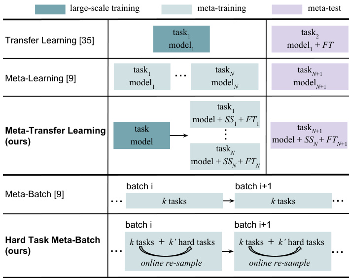
Figure 1. Meta-transfer learning (MTL) is our meta-learning paradigm and hard task (HT) meta-batch is our training strategy. The upper three rows show the differences between MTL and related methods, transfer-learning [35] and meta-learning [9]. The bottom rows compare HT meta-batch with the conventional metabatch [9]. $F T$ stands for fine-tuning a classifier. SS represents the Scaling and Shifting operations in our MTL method.

图 1: 元迁移学习 (MTL) 是我们的元学习范式，而困难任务 (HT) 元批次是我们的训练策略。前三行展示了 MTL 与相关方法 (迁移学习 [35] 和元学习 [9]) 的区别。底部几行比较了 HT 元批次与传统元批次 [9]。$FT$ 表示微调分类器。SS 代表我们 MTL 方法中的缩放和移位操作。

Few-shot learning methods can be roughly categorized into two classes: data augmentation and task-based metalearning. Data augmentation is a classic technique to increase the amount of available data and thus also useful for few-shot learning [21]. Several methods propose to learn a data generator e.g. conditioned on Gaussian noise [29, 44, 54]. However, the generation models often under perform when trained on few-shot data [1]. An alternative is to merge data from multiple tasks which, however, is not effective due to variances of the data across tasks [54].

少样本学习方法大致可分为两类：数据增强和基于任务的元学习。数据增强是增加可用数据量的经典技术，因此对少样本学习也很有用 [21]。一些方法提出学习数据生成器，例如以高斯噪声为条件 [29, 44, 54]。然而，当在少样本数据上训练时，生成模型通常表现不佳 [1]。另一种方法是合并来自多个任务的数据，但由于任务间数据的差异，这种方法效果不佳 [54]。

In contrast to data-augmentation methods, meta-learning is a task-level learning method [2, 33, 52]. Meta-learning aims to accumulate experience from learning multiple tasks [9, 39, 48, 31, 13], while base-learning focuses on modeling the data distribution of a single task. A state-of-theart representative of this, namely Model-Agnostic MetaLearning (MAML), learns to search for the optimal initialization state to fast adapt a base-learner to a new task [9]. Its task-agnostic property makes it possible to generalize to few-shot supervised learning as well as unsupervised reinforcement learning [13, 10]. However, in our view, there are two main limitations of this type of approaches limiting their effectiveness: i) these methods usually require a large number of similar tasks for meta-training which is costly; and ii) each task is typically modeled by a lowcomplexity base learner (such as a shallow neural network) to avoid model over fitting, thus being unable to use deeper and more powerful architectures. For example, for the miniImageNet dataset [53], MAML uses a shallow CNN with only 4 CONV layers and its optimal performance was obtained learning on $240k$ tasks.

与数据增强方法不同，元学习是一种任务级学习方法 [2, 33, 52]。元学习旨在从多个任务中积累经验 [9, 39, 48, 31, 13]，而基础学习则专注于建模单个任务的数据分布。该领域的先进代表模型——模型无关元学习 (Model-Agnostic Meta-Learning, MAML) 通过学习搜索最优初始化状态，使基础学习器能够快速适应新任务 [9]。其任务无关特性使其能够泛化到少样本监督学习以及无监督强化学习 [13, 10]。然而，我们认为这类方法存在两个主要局限性：i) 这些方法通常需要大量相似任务进行元训练，成本高昂；ii) 每个任务通常由低复杂度基础学习器 (如浅层神经网络) 建模以避免过拟合，因此无法使用更深层、更强大的架构。例如，在 miniImageNet 数据集 [53] 上，MAML 仅使用 4 层卷积的浅层 CNN，并通过学习 $240k$ 个任务才获得最佳性能。

In this paper, we propose a novel meta-learning method called meta-transfer learning (MTL) leveraging the advantages of both transfer and meta learning (see conceptual comparison of related methods in Figure 1). In a nutshell, MTL is a novel learning method that helps deep neural nets converge faster while reducing the probability to overfit when using few labeled training data only. In particular, “transfer” means that DNN weights trained on largescale data can be used in other tasks by two light-weight neuron operations: Scaling and Shifting (SS), i.e. $\alpha X+\beta$ . “Meta” means that the parameters of these operations can be viewed as hyper-parameters trained on few-shot learning tasks [31, 26]. Large-scale trained DNN weights of- fer a good initialization, enabling fast convergence of metatransfer learning with fewer tasks, e.g. only $8k$ tasks for mini Image Net [53], 30 times fewer than MAML [9]. Lightweight operations on DNN neurons have less parameters to learn, e.g. less than $\textstyle{\frac{2}{49}}$ if considering neurons of size $7\times7$ $\frac{1}{49}$ for $\alpha$ and $<\frac{1}{49}$ for $\beta$ ), reducing the chance of overfitting. In addition, these operations keep those trained DNN weights unchanged, and thus avoid the problem of “catastrophic forgetting” which means forgetting general patterns when adapting to a specific task [27, 28].

本文提出了一种名为元迁移学习(MTL)的新型元学习方法，该方法结合了迁移学习和元学习的优势(相关方法的概念对比见图1)。简而言之，MTL是一种新颖的学习方法，能够在仅使用少量标注训练数据时，帮助深度神经网络更快收敛并降低过拟合概率。具体而言，"迁移"是指通过两个轻量级的神经元操作——缩放与平移(SS)，即$\alpha X+\beta$，将在大规模数据上训练的DNN权重应用于其他任务。"元"则意味着这些操作的参数可视为在少样本学习任务上训练的超参数[31,26]。大规模训练的DNN权重提供了良好的初始化，使得元迁移学习能以更少的任务实现快速收敛，例如在mini ImageNet上仅需$8k$个任务[53]，比MAML少30倍[9]。对DNN神经元的轻量级操作需要学习的参数更少(例如对于$7\times7$大小的神经元，$\alpha$参数少于$\textstyle{\frac{2}{49}}$，$\beta$参数少于$\frac{1}{49}$)，从而降低了过拟合风险。此外，这些操作保持已训练的DNN权重不变，因此避免了"灾难性遗忘"问题——即在适应特定任务时遗忘通用模式的现象[27,28]。

The second main contribution of this paper is an effective meta-training curriculum. Curriculum learning [3] and hard negative mining [47] both suggest that faster convergence and stronger performance can be achieved by a better arrangement of training data. Inspired by these ideas, we design our hard task (HT) meta-batch strategy to offer a challenging but effective learning curriculum. As shown in the bottom rows of Figure 1, a conventional meta-batch contains a number of random tasks [9], but our HT meta-batch online re-samples harder ones according to past failure tasks with lowest validation accuracy.

本文的第二个主要贡献是提出了一种高效的元训练课程。课程学习 [3] 和难负例挖掘 [47] 都表明，通过更好地安排训练数据可以实现更快的收敛和更强的性能。受这些思想的启发，我们设计了难任务 (HT) 元批次策略，以提供一个具有挑战性但高效的学习课程。如图 1 底部行所示，传统的元批次包含多个随机任务 [9]，而我们的 HT 元批次会根据验证准确率最低的过去失败任务在线重新采样更难的任务。

Our overall contribution is thus three-fold: i) we propose a novel MTL method that learns to transfer largescale pre-trained DNN weights for solving few-shot learning tasks; ii) we propose a novel HT meta-batch learning strategy that forces meta-transfer to “grow faster and stronger through hardship”; and iii) we conduct extensive experiments on two few-shot learning benchmarks, namely mini Image Net [53] and Fewshot-CIFAR100 (FC100) [34], and achieve the state-of-the-art performance.

我们的总体贡献体现在三个方面：i) 提出一种新颖的多任务学习 (MTL) 方法，通过迁移大规模预训练深度神经网络 (DNN) 权重来解决少样本学习任务；ii) 提出创新的硬训练 (HT) 元批量学习策略，迫使元迁移"通过逆境更快更强地成长"；iii) 在两个少样本学习基准测试（mini ImageNet [53] 和 Fewshot-CIFAR100 (FC100) [34]）上进行了广泛实验，并实现了最先进的性能。

2. Related work

2. 相关工作

Few-shot learning Research literature on few-shot learning exhibits great diversity. In this section, we focus on methods using the supervised meta-learning paradigm [12, 52, 9] most relevant to ours and compared to in the experiments. We can divide these methods into three categories. 1) Metric learning methods [53, 48, 51] learn a similarity space in which learning is efficient for few-shot examples. 2) Memory network methods [31, 42, 34, 30] learn to store “experience” when learning seen tasks and then generalize that to unseen tasks. 3) Gradient descent based methods [9, 39, 24, 13, 60] have a specific meta-learner that learns to adapt a specific base-learner (to few-shot examples) through different tasks. E.g. MAML [9] uses a meta-learner that learns to effectively initialize a base-learner for a new learning task. Meta-learner optimization is done by gradient descent using the validation loss of the base-learner. Our method is closely related. An important difference is that our MTL approach leverages transfer learning and benefits from referencing neuron knowledge in pre-trained deep nets. Although MAML can start from a pre-trained network, its element-wise fine-tuning makes it hard to learn deep nets without over fitting (validated in our experiments). Transfer learning What and how to transfer are key issues to be addressed in transfer learning, as different methods are applied to different source-target domains and bridge different transfer knowledge [35, 57, 55, 59]. For deep models, a powerful transfer method is adapting a pre-trained model for a new task, often called fine-tuning $(F T)$ . Models pretrained on large-scale datasets have proven to generalize better than randomly initialized ones [8]. Another popular transfer method is taking pre-trained networks as backbone and adding high-level functions, e.g. for object detection and recognition [18, 50, 49] and image segmentation [16, 5]. Our meta-transfer learning leverages the idea of transferring pre-trained weights and aims to meta-learn how to effectively transfer. In this paper, large-scale trained DNN weights are what to transfer, and the operations of Scaling and Shifting indicate how to transfer. Similar operations have been used to modulating the per-feature-map distribution of activation s for visual reasoning [37].

少样本学习
关于少样本学习的研究文献呈现出极大的多样性。本节重点讨论与我们的方法最相关且在实验中进行了对比的监督元学习范式 [12, 52, 9] 相关方法。这些方法可分为三类：

1. 度量学习方法 [53, 48, 51] 通过学习一个相似性空间，使得少样本示例能高效学习；
2. 记忆网络方法 [31, 42, 34, 30] 通过学习存储已见任务的"经验"，进而泛化到未见任务；
3. 基于梯度下降的方法 [9, 39, 24, 13, 60] 通过特定元学习器，在不同任务中学习如何适配基础学习器（以适应少样本示例）。例如 MAML [9] 使用元学习器来学习如何为新学习任务有效初始化基础学习器，其优化通过基础学习器的验证损失进行梯度下降实现。

我们的方法与之密切相关，但关键区别在于：多任务学习 (MTL) 方法利用了迁移学习，并受益于预训练深度网络中的神经元知识引用。尽管 MAML 可以从预训练网络开始，但其逐元素微调特性使其难以在不发生过拟合的情况下学习深度网络（实验已验证）。

迁移学习
迁移内容和迁移方式是迁移学习需要解决的核心问题 [35, 57, 55, 59]，因为不同方法适用于不同源-目标域并桥接不同的迁移知识。对于深度模型，强大的迁移方法是针对新任务调整预训练模型，通常称为微调 $(F T)$ 。实践证明，在大规模数据集上预训练的模型比随机初始化模型具有更好的泛化能力 [8]。另一种流行迁移方法是将预训练网络作为主干并添加高级功能，例如用于目标检测与识别 [18, 50, 49] 和图像分割 [16, 5]。

我们的元迁移学习借鉴了迁移预训练权重的思想，旨在元学习如何有效迁移。本文中，大规模训练的 DNN 权重是迁移内容，而缩放 (Scaling) 和偏移 (Shifting) 操作则指明了迁移方式。类似操作曾用于调节视觉推理中激活的逐特征图分布 [37]。

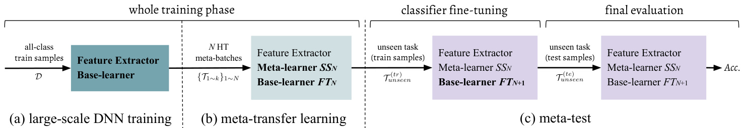
Figure 2. The pipeline of our proposed few-shot learning method, including three phases: (a) DNN training on large-scale data, i.e. using all training datapoints (Section 4.1); (b) Meta-transfer learning (MTL) that learns the parameters of Scaling and Shifting (SS), based on the pre-trained feature extractor (Section 4.2). Learning is scheduled by the proposed HT meta-batch (Section 4.3); and (c) meta-test is done for an unseen task which consists of a base-learner (classifier) Fine-Tuning $(F T)$ stage and a final evaluation stage, described in the last paragraph in Section 3. Input data are along with arrows. Modules with names in bold get updated at corresponding phases. Specifically, SS parameters are learned by meta-training but fixed during meta-test. Base-learner parameters are optimized for every task.

图 2: 我们提出的少样本学习方法的流程，包括三个阶段：(a) 在大规模数据上训练DNN，即使用所有训练数据点（第4.1节）；(b) 基于预训练特征提取器的元迁移学习 (MTL)，学习缩放和位移 (SS) 的参数（第4.2节）。学习过程由提出的HT元批次调度（第4.3节）；(c) 对未见任务进行元测试，包括基础学习器（分类器）微调 $(F T)$ 阶段和最终评估阶段，如第3节最后一段所述。输入数据沿箭头方向流动。名称加粗的模块在相应阶段更新。具体而言，SS参数通过元训练学习，但在元测试期间固定。基础学习器参数针对每个任务进行优化。

Some few-shot learning methods have been proposed to use pre-trained weights as initialization [20, 30, 38, 45, 41]. Typically, weights are fine-tuned for each task, while we learn a meta-transfer learner through all tasks, which is dif ferent in terms of the underlying learning paradigm.

一些少样本学习方法提出使用预训练权重作为初始化 [20, 30, 38, 45, 41]。通常权重会针对每个任务进行微调，而我们通过所有任务学习一个元迁移学习器，这在底层学习范式上有所不同。

Curriculum learning & Hard sample mining Curriculum learning was proposed by Bengio et al. [3] and is popular for multi-task learning [36, 43, 56, 14]. They showed that instead of observing samples at random it is better to organize samples in a meanin(gmfetua-lle arwnera)y so that fast convergence, effective learning and better generalization can be achieved. Pentina et al. [36] use adaptive SVM class if i ers to evaluate task difficulty for later organization. Differently, our MTL method does task evaluation online at the phase of episode test, without needing any auxiliary model.

课程学习与困难样本挖掘
课程学习由Bengio等人[3]提出，在多任务学习领域广受欢迎[36,43,56,14]。研究表明，相较于随机观察样本，以有意义的方式组织样本能实现更快收敛、更高效学习和更优泛化性能。Pentina等人[36]采用自适应SVM分类器评估任务难度以进行后续组织。与之不同，我们的多任务学习方法在片段测试阶段在线评估任务，无需任何辅助模型。

Hard sample mining was proposed by Shri vast ava et al. [47] for object detection. It treats image proposals overlapped with ground truth as hard negative samples. Training on more confusing data enables the model to achieve higher robustness and better performance [4, 15, 7]. Inspired by this, we sample harder tasks online and make our MTL learner “grow faster and stronger through more hardness”. In our experiments, we show that this can be generalized to enhance other meta-learning methods, e.g. MAML [9].

难样本挖掘由Shrivastava等人[47]提出用于目标检测。该方法将与真实标注框重叠的图像候选区域视为难负样本。在更具挑战性的数据上训练能使模型获得更高鲁棒性和更好性能[4,15,7]。受此启发，我们在线采样更难的任务，使多任务学习器"通过更大难度成长得更快更强"。实验表明该方法可推广至增强其他元学习方法，例如MAML[9]。

ing a set of unseen datapoints $\mathcal{T}_{u n s e e n}^{(t e)}$

对一组未见数据点 $\mathcal{T}_{u n s e e n}^{(t e)}$ 进行处理

Meta-training phase. This phase aims to learn a metalearner from θ’multiple episodes. In each episode, metatraining has a two-stage optimization. Stage-1 is called base-learning, where the cross-entropy loss is used to optimize the parameters of the base-learner. Stage-2 contains a feed-forward test on episode test datapoints. The test loss is used to optimize the parameters of the meta-learner. Specifically, given an episode $\mathcal{T}\in p(\mathcal{T})$ , the base-learner $\theta_{T}$ is learned from episode training data $\mathcal{T}^{(t r)}$ and its corresponding loss $\mathcal{L}{\mathcal{T}}(\theta_{\mathcal{T}},\mathcal{T}^{(t r)})$ . After optimizing this loss, the baselearner has parameters $\tilde{\theta}{T}$ . Then, the meta-learner is updated using test loss $\mathcal{L}{\mathcal{T}}(\tilde{\theta}{\mathcal{T}},\mathcal{T}^{(t e)})$ . After meta-training on all episodes, the meta-learner is optimized by test losses ${\mathcal{L}{\mathcal{T}}(\tilde{\theta}{\mathcal{T}},\mathcal{T}^{(t e)})}_{\mathcal{T}\in p(\mathcal{T})}$ . Therefore, the number of metalearner updates equals to the number of episodes.

元训练阶段。该阶段旨在从θ的多个情节中学习元学习器。每个情节的元训练包含两阶段优化：第一阶段称为基础学习，使用交叉熵损失优化基础学习器参数；第二阶段对情节测试数据点进行前馈测试，利用测试损失优化元学习器参数。具体而言，给定情节$\mathcal{T}\in p(\mathcal{T})$时，基础学习器$\theta_{T}$从情节训练数据$\mathcal{T}^{(t r)}$及其对应损失$\mathcal{L}{\mathcal{T}}(\theta_{\mathcal{T}},\mathcal{T}^{(t r)})$中学习。优化该损失后，基础学习器获得参数$\tilde{\theta}{T}$，随后使用测试损失$\mathcal{L}{\mathcal{T}}(\tilde{\theta}{\mathcal{T}},\mathcal{T}^{(t e)})$更新元学习器。在所有情节完成元训练后，元学习器通过测试损失集合${\mathcal{L}{\mathcal{T}}(\tilde{\theta}{\mathcal{T}},\mathcal{T}^{(t e)})}_{\mathcal{T}\in p(\mathcal{T})}$完成优化，因此元学习器的更新次数等于情节数量。

Meta-test phase. This phase aims to test the performance of the trained meta-learner for fast adaptation to unseen task. Given $\tau_{u n s e e n}$ , the meta-learner $\tilde{\theta}{T}$ teaches the baselearner θ unseen to adapt to the objective of $\tau_{u n s e e n}$ by some means, e.g. through initialization [9]. Then, the test result on $\mathcal{T}{u n s e e n}^{(t e)}$ is used to evaluate the meta-learning approach. If there are multiple unseen tasks ${\mathcal{T}{u n s e e n}}$ , the average result on ${\mathcal{T}_{u n s e e n}^{(t e)}}$ will be the final evaluation.

元测试阶段。该阶段旨在测试训练好的元学习器 (meta-learner) 对未见任务 (unseen task) 的快速适应性能。给定 $\tau_{u n s e e n}$ ，元学习器 $\tilde{\theta}{T}$ 会通过某种方式 (例如初始化 [9]) 指导基学习器 (baselearner) θ unseen 适应 $\tau_{u n s e e n}$ 的目标。随后，在 $\mathcal{T}{u n s e e n}^{(t e)}$ 上的测试结果将用于评估元学习方法。若存在多个未见任务 ${\mathcal{T}{u n s e e n}}$ ，则 ${\mathcal{T}_{u n s e e n}^{(t e)}}$ 上的平均结果将作为最终评估依据。

3. Preliminary

3. 初步准备

We introduce the problem setup and notations of metalearning, following related work [53, 39, 9, 34].

我们引入元学习的问题设置和符号表示，相关工作见[53, 39, 9, 34]。

Meta-learning consists of two phases: meta-train and meta-test. A meta-training example is a classification task $\tau$ sampled from a distribution $p(\mathcal T)$ . $\tau$ is called episode, including a training split $\mathcal{T}^{(t r)}$ to optimize the base-learner, and a test split $\boldsymbol{\mathcal{T}^{(t e)}}$ to optimize the meta-learner. In particular, meta-training aims to learn from a number of episodes ${\mathcal{T}}$ sampled from $p(\mathcal{T})$ . An unseen task $\tau_{u n s e e n}$ in metatest will start from that experience of the meta-learner and adapt the base-learner. The final evaluation is done by test

元学习包含两个阶段：元训练和元测试。一个元训练样本是从分布 $p(\mathcal T)$ 中采样的分类任务 $\tau$。$\tau$ 称为情节(episode)，包含用于优化基础学习器的训练集 $\mathcal{T}^{(t r)}$，以及用于优化元学习器的测试集 $\boldsymbol{\mathcal{T}^{(t e)}}$。具体而言，元训练旨在从 $p(\mathcal{T})$ 采样的多个情节 ${\mathcal{T}}$ 中学习。在元测试中，未见任务 $\tau_{u n s e e n}$ 将从元学习器的经验出发，并适配基础学习器。最终评估通过测试完成。

4. Methodology

4. 方法论

As shown in Figure 2, our method consists of three phases. First, we train a DNN on large-scale data, e.g. on mini Image Net (64-class, 600-shot) [53], and then fix the low-level layers as Feature Extractor (Section 4.1). Second, in the meta-transfer learning phase, MTL learns the Scaling and Shifting (SS) parameters for the Feature Extractor neurons, enabling fast adaptation to few-shot tasks (Section 4.2). For improved overall learning, we use our HT meta-batch strategy (Section 4.3). The training steps are detailed in Algorithm 1 in Section 4.4. Finally, the typical meta-test phase is performed, as introduced in Section 3.

如图 2 所示，我们的方法包含三个阶段。首先，我们在大规模数据上训练深度神经网络 (DNN)，例如 mini Image Net (64 类，600-shot) [53]，然后固定底层作为特征提取器 (第 4.1 节)。其次，在元迁移学习阶段，MTL 学习特征提取神经元的缩放和移位 (SS) 参数，实现快速适应少样本任务 (第 4.2 节)。为提升整体学习效果，我们采用 HT 元批次策略 (第 4.3 节)。训练步骤详见第 4.4 节的算法 1。最后执行典型的元测试阶段，如第 3 节所述。

4.1. DNN training on large-scale data

4.1. 大规模数据上的DNN训练

This phase is similar to the classic pre-training stage as, e.g., pre-training on Imagenet for object recognition [40]. Here, we do not consider data/domain adaptation from other datasets, and pre-train on readily available data of few-shot learning benchmarks, allowing for fair comparison with other few-shot learning methods. Specifically, for a particular few-shot dataset, we merge all-class data $\mathcal{D}$ for pretraining. For instance, for mini Image Net [53], there are totally 64 classes in the training split of $\mathcal{D}$ and each class contains 600 samples used to pre-train a 64-class classifier.

这一阶段类似于经典的预训练阶段，例如在Imagenet上进行物体识别的预训练[40]。在此，我们不考虑从其他数据集进行数据/领域适应，而是直接在现成的少样本学习基准数据上进行预训练，以便与其他少样本学习方法进行公平比较。具体而言，对于特定的少样本数据集，我们合并所有类别的数据$\mathcal{D}$进行预训练。例如，对于mini ImageNet[53]，训练集$\mathcal{D}$中共有64个类别，每个类别包含600个样本，用于预训练一个64类分类器。

We first randomly initialize a feature extractor $\Theta$ (e.g. CONV layers in ResNets [17]) and a classifier $\theta$ (e.g. the last FC layer in ResNets [17]), and then optimize them by gradient descent as follows,

我们首先随机初始化一个特征提取器 $\Theta$ （例如 ResNets [17] 中的 CONV 层）和一个分类器 $\theta$ （例如 ResNets [17] 中的最后一个 FC 层），然后通过梯度下降优化它们，具体步骤如下，

$$
\begin{array}{r}{[\Theta;\theta]=:\left[\Theta;\theta\right]-\alpha\nabla\mathcal{L}_{\mathcal{D}}\left([\Theta;\theta]\right),}\end{array}
$$

$$
\begin{array}{r}{[\Theta;\theta]=:\left[\Theta;\theta\right]-\alpha\nabla\mathcal{L}_{\mathcal{D}}\left([\Theta;\theta]\right),}\end{array}
$$

where $\mathcal{L}$ denotes the following empirical loss,

其中 $\mathcal{L}$ 表示以下经验损失，

$$
\mathcal{L}{\mathcal{D}}\big([\Theta;\theta]\big)=\frac{1}{|\mathcal{D}|}\sum_{(x,y)\in\mathcal{D}}l\big(f_{[\Theta;\theta]}(x),y\big),
$$

$$
\mathcal{L}{\mathcal{D}}\big([\Theta;\theta]\big)=\frac{1}{|\mathcal{D}|}\sum_{(x,y)\in\mathcal{D}}l\big(f_{[\Theta;\theta]}(x),y\big),
$$

e.g. cross-entropy loss, and $\alpha$ denotes the learning rate. In this phase, the feature extractor $\Theta$ is learned. It will be frozen in the following meta-training and meta-test phases, as shown in Figure 2. The learned classifier $\theta$ will be discarded, because subsequent few-shot tasks contain different classification objectives, e.g. 5-class instead of 64-class classification for mini Image Net [53].

例如交叉熵损失 (cross-entropy loss)，而 $\alpha$ 表示学习率。在此阶段，特征提取器 $\Theta$ 被学习。它将在后续的元训练和元测试阶段被冻结，如图 2 所示。学习到的分类器 $\theta$ 将被丢弃，因为后续的少样本任务包含不同的分类目标，例如 mini ImageNet [53] 中的 5 类分类而非 64 类分类。

4.2. Meta-transfer learning (MTL)

4.2. 元迁移学习 (MTL)

As shown in Figure 2(b), our proposed meta-transfer learning (MTL) method optimizes the meta operations Scaling and Shifting (SS) through HT meta-batch training (Section 4.3). Figure 3 visualizes the difference of updating through SS and $F T,S S$ operations, denoted as $\Phi_{S_{1}}$ and $\Phi_{S_{2}}$ do not change the frozen neuron weights of $\Theta$ during learning, while $F T$ updates the complete $\Theta$ .

如图 2(b) 所示, 我们提出的元迁移学习 (meta-transfer learning, MTL) 方法通过 HT 元批次训练 (第 4.3 节) 优化元操作缩放与平移 (Scaling and Shifting, SS)。图 3 展示了通过 SS 和 $F T,S S$ 操作进行更新的差异, 记为 $\Phi_{S_{1}}$ 和 $\Phi_{S_{2}}$ 在学习过程中不会改变 $\Theta$ 的冻结神经元权重, 而 $F T$ 会更新完整的 $\Theta$。

In the following, we detail the $S S$ operations. Given a task $\tau$ , the loss of $\mathcal{T}^{(t r)}$ is used to optimize the current base-learner (classifier) $\theta^{\prime}$ by gradient descent:

下面我们详细介绍 $S S$ 操作。给定任务 $\tau$，通过梯度下降使用 $\mathcal{T}^{(t r)}$ 的损失来优化当前基础学习器（分类器） $\theta^{\prime}$：

$$
\theta^{\prime}\leftarrow\theta-\beta\nabla_{\theta}\mathcal{L}{\mathcal{T}^{(t r)}}\big([\Theta;\theta],\Phi_{S_{{1,2}}}\big),
$$

$$
\theta^{\prime}\leftarrow\theta-\beta\nabla_{\theta}\mathcal{L}{\mathcal{T}^{(t r)}}\big([\Theta;\theta],\Phi_{S_{{1,2}}}\big),
$$

which is different to Eq. 1, as we do not update $\Theta$ . Note that here $\theta$ is different to the one from the previous phase, the large-scale classifier $\theta$ in Eq. 1. This $\theta$ concerns only a few of classes, e.g. 5 classes, to classify each time in a novel few-shot setting. $\theta^{\prime}$ corresponds to a temporal classifier only working in the current task, initialized by the $\theta$ optimized for the previous task (see Eq. 5).

这与式1不同，因为我们不更新$\Theta$。请注意，这里的$\theta$与前一阶段的不同，即式1中的大规模分类器$\theta$。这个$\theta$仅涉及少量类别（例如5类），在每次少样本新任务中进行分类。$\theta^{\prime}$对应一个仅在当前任务中工作的临时分类器，由针对前一任务优化的$\theta$初始化（见式5）。

$\Phi_{S_{1}}$ is initialized by ones and $\Phi_{S_{1}}$ by zeros. Then, they are optimized by the test loss of $\mathcal{T}^{(t e)}$ as follows,

$\Phi_{S_{1}}$ 初始化为1，$\Phi_{S_{1}}$ 初始化为0。然后，通过 $\mathcal{T}^{(t e)}$ 的测试损失对它们进行如下优化：

$$
\Phi_{S_{i}}=:\Phi_{S_{i}}-\gamma\nabla_{\Phi_{S_{i}}}\mathcal{L}{\mathcal{T}^{(t e)}}\left([\Theta;\theta^{\prime}],\Phi_{S_{{1,2}}}\right).
$$

$$
\Phi_{S_{i}}=:\Phi_{S_{i}}-\gamma\nabla_{\Phi_{S_{i}}}\mathcal{L}{\mathcal{T}^{(t e)}}\left([\Theta;\theta^{\prime}],\Phi_{S_{{1,2}}}\right).
$$

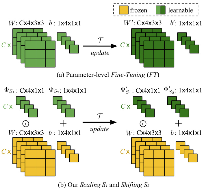
Figure 3. (a) Parameter-level Fine-Tuning $(F T)$ is a conventional meta-training operation, e.g. in MAML [9]. Its update works for all neuron parameters, $W$ and $^b$ . (b) Our neuron-level Scaling and Shifting (SS) operations in MTL. They reduce the number of learning parameters and avoid over fitting problems. In addition, they keep large-scale trained parameters (in yellow) frozen, preventing “catastrophic fogetting” [27, 28].

图 3: (a) 参数级微调 (FT) 是传统元训练操作 (例如 MAML [9]), 其更新作用于所有神经元参数 $W$ 和 $^b$。 (b) 我们在 MTL 中提出的神经元级缩放与平移 (SS) 操作。该操作减少了学习参数量并避免过拟合问题, 同时保持大规模训练参数 (黄色部分) 固定, 从而防止"灾难性遗忘" [27, 28]。

In this step, $\theta$ is updated with the same learning rate $\gamma$ as in Eq. 4,

在这一步中，$\theta$ 以与式4中相同的学习率 $\gamma$ 进行更新，

$$
\theta=:\theta-\gamma\nabla_{\theta}\mathcal{L}{\mathcal{T}^{(t e)}}\left([\Theta;\theta^{\prime}],\Phi_{S_{{1,2}}}\right).
$$

$$
\theta=:\theta-\gamma\nabla_{\theta}\mathcal{L}{\mathcal{T}^{(t e)}}\left([\Theta;\theta^{\prime}],\Phi_{S_{{1,2}}}\right).
$$

Re-linking to Eq. 3, we note that the above $\theta^{\prime}$ comes from the last epoch of base-learning on $\mathcal{T}^{(t r)}$ .

重新关联到式3，我们注意到上述 $\theta^{\prime}$ 来自基于 $\mathcal{T}^{(t r)}$ 的基础学习最后一个周期。

Next, we describe how we apply $\Phi_{S_{{1,2}}}$ to the frozen neurons as shown in Figure 3(b). Given the trained $\Theta$ , for its $l$ -th layer containing $K$ neurons, we have $K$ pairs of parameters, respectively as weight and bias, denoted as ${(W_{i,k},b_{i,k})}$ . Note that the neuron location $l,k$ will be omitted for readability. Based on MTL, we learn $K$ pairs of scalars ${\Phi_{S_{{1,2}}}}$ . Assuming $X$ is input, we apply ${\Phi_{S_{{1,2}}}}$ to $(W,b)$ as

接下来，我们描述如何将 $\Phi_{S_{{1,2}}}$ 应用于冻结神经元，如图 3(b) 所示。给定训练好的 $\Theta$，对于包含 $K$ 个神经元的第 $l$ 层，我们有 $K$ 对参数（分别为权重和偏置），记为 ${(W_{i,k},b_{i,k})}$。注意，为便于阅读，神经元位置 $l,k$ 将被省略。基于多任务学习 (MTL)，我们学习 $K$ 对标量 ${\Phi_{S_{{1,2}}}}$。假设 $X$ 是输入，我们将 ${\Phi_{S_{{1,2}}}}$ 应用于 $(W,b)$，公式为

$$
S S(X;W,b;\Phi_{S_{{1,2}}})=(W\odot\Phi_{S_{1}})X+(b+\Phi_{S_{2}}),
$$

$$
S S(X;W,b;\Phi_{S_{{1,2}}})=(W\odot\Phi_{S_{1}})X+(b+\Phi_{S_{2}}),
$$

where $\odot$ denotes the element-wise multiplication

其中 $\odot$ 表示逐元素相乘

Taking Figure 3(b) as an example of a single $3\times3$ filter, after SS operations, this filter is scaled by $\Phi_{S_{1}}$ then the feature maps after convolutions are shifted by $\Phi_{S_{2}}$ in addition to the original bias $b$ . Detailed steps of SS are given in Algorithm 2 in Section 4.4.

以图 3(b) 中的单个 $3\times3$ 滤波器为例，经过 SS (scale and shift) 操作后，该滤波器先由 $\Phi_{S_{1}}$ 进行缩放，随后卷积得到的特征图会在原始偏置 $b$ 基础上再偏移 $\Phi_{S_{2}}$ 。具体步骤详见第 4.4 节算法 2。

Figure 3(a) shows a typical parameter-level Fine-Tuning $(F T)$ operation, which is in the meta optimization phase of our related work MAML [9]. It is obvious that $F T$ updates the complete values of $W$ and $b$ , and has a large number of parameters, and our SS reduces this number to below $\frac{2}{9}$ in the example of the figure.

图 3(a) 展示了一个典型的参数级微调 $(F T)$ 操作，该操作处于我们相关工作 MAML [9] 的元优化阶段。显然 $F T$ 会完整更新 $W$ 和 $b$ 的数值，且参数量较大，而我们的 SS 方法在该图示例中将参数量降低至 $\frac{2}{9}$ 以下。

In summary, SS can benefit MTL in three aspects. 1) It starts from a strong initialization based on a large-scale trained DNN, yielding fast convergence for MTL. 2) It does not change DNN weights, thereby avoiding the problem of “catastrophic forgetting” [27, 28] when learning specific tasks in MTL. 3) It is light-weight, reducing the chance of over fitting of MTL in few-shot scenarios.

总结来说，SS可以从三个方面使多任务学习(MTL)受益。1) 它基于大规模训练过的深度神经网络(DNN)进行强初始化，从而为MTL带来快速收敛。2) 它不会改变DNN的权重，因此避免了在MTL中学习特定任务时出现"灾难性遗忘" [27, 28]的问题。3) 它是轻量级的，降低了MTL在少样本场景下过拟合的可能性。

4.3. Hard task (HT) meta-batch

4.3. 困难任务 (HT) 元批次

In this section, we introduce a method to schedule hard tasks in meta-training batches. The conventional metabatch is composed of randomly sampled tasks, where the randomness implies random difficulties [9]. In our metatraining pipeline, we intentionally pick up failure cases in each task and re-compose their data to be harder tasks for adverse re-training. We aim to force our meta-learner to “grow up through hardness”.

在本节中，我们介绍了一种在元训练批次中调度硬任务的方法。传统元批次由随机抽样的任务组成，这种随机性意味着任务难度也是随机的 [9]。在我们的元训练流程中，我们有意选取每个任务中的失败案例，并将其数据重新组合成更困难的任务用于对抗性再训练。我们的目标是迫使元学习器"在困难中成长"。

Pipeline. Each task $\tau$ has two splits, $\mathcal{T}^{(t r)}$ and $\mathcal{T}^{(t e)}$ , for base-learning and test, respectively. As shown in Algorithm 2 line 2-5, base-learner is optimized by the loss of $\mathcal{T}^{(t r)}$ (in multiple epochs). SS parameters are then optimized by the loss of $\mathcal{T}^{(t e)}$ once. We can also get the recognition accuracy of $\mathcal{T}^{(t e)}$ for $M$ classes. Then, we choose the lowest accuracy $A c c_{m}$ to determine the most difficult class $\cdot m$ (also called failure class) in the current task.

流程。每个任务 $\tau$ 包含两个数据分割 $\mathcal{T}^{(tr)}$ 和 $\mathcal{T}^{(te)}$ ，分别用于基础学习和测试。如算法2第2-5行所示，基础学习器通过 $\mathcal{T}^{(tr)}$ 的损失进行多轮优化 (multiple epochs) ，随后SS参数通过 $\mathcal{T}^{(te)}$ 的损失单次优化。我们还能获得 $\mathcal{T}^{(te)}$ 在 $M$ 个类别上的识别准确率，进而选取最低准确率 $Acc_m$ 来确定当前任务中最困难的类别 $\cdot m$ (亦称失败类别) 。

After obtaining all failure classes (indexed by ${m}$ ) from $k$ tasks in current meta-batch ${\mathcal T_{1\sim k}}$ , we re-sample tasks from their data. Specifically, we assume $p(\mathcal{T}|{m})$ is the task distribution, we sample a “harder” task ${\mathcal{T}}^{h a r d}\in$ $p(\mathcal{T}|{m})$ . Two important details are given below.

在当前元批次 ${\mathcal T_{1\sim k}}$ 中从 $k$ 个任务获取所有故障类别 (索引为 ${m}$) 后，我们从其数据中重新采样任务。具体而言，假设 $p(\mathcal{T}|{m})$ 是任务分布，我们从中采样一个"更难"的任务 ${\mathcal{T}}^{hard}\in p(\mathcal{T}|{m})$。以下是两个重要细节说明。

Choosing hard class $m$ . We choose the failure class $\cdot m$ from each task by ranking the class-level accuracies instead of fixing a threshold. In a dynamic online setting as ours, it is more sensible to choose the hardest cases based on ranking rather than fixing a threshold ahead of time.

选择困难类别$m$。我们通过按类别准确率排序而非固定阈值的方式，从每个任务中选出失败类别$\cdot m$。在我们这种动态在线场景中，基于排序选择最困难案例比预先固定阈值更为合理。

Two methods of hard tasking using ${m}$ . Chosen ${m}$ , we can re-sample tasks $\mathcal{T}^{h a r d}$ by (1) directly using the samples of class $\cdot m$ in the current task $\tau$ , or (2) indirectly using the label of class $\cdot m$ to sample new samples of that class. In fact, setting (2) considers to include more data variance of class $\cdot m$ and it works better than setting (1) in general.

使用 ${m}$ 进行困难任务处理的两种方法。选定 ${m}$ 后，我们可以通过以下方式对任务 $\mathcal{T}^{hard}$ 进行重采样：(1) 直接使用当前任务 $\tau$ 中类别 $\cdot m$ 的样本，或 (2) 间接利用类别 $\cdot m$ 的标签采样该类别的新样本。实际上，设置(2)考虑了包含更多类别 $\cdot m$ 的数据方差，通常比设置(1)效果更好。

4.4. Algorithm

4.4. 算法

Algorithm 1 summarizes the training process of two main stages: large-scale DNN training (line 1-5) and metatransfer learning (line 6-22). HT meta-batch re-sampling and continuous training phases are shown in lines 16-20, for which the failure classes are returned by Algorithm 2, see line 14. Algorithm 2 presents the learning process on a single task that includes episode training (lines 2-5) and episode test, i.e. meta-level update (lines 6). In lines 7-11, the recognition rates of all test classes are computed and returned to Algorithm 1 (line 14) for hard task sampling.

算法1总结了两大阶段的训练过程：大规模DNN训练（第1-5行）和元迁移学习（第6-22行）。其中第16-20行展示了HT元批次重采样和持续训练阶段，其失败类别由算法2返回（见第14行）。算法2呈现了单任务学习流程，包含片段训练（第2-5行）和片段测试即元级更新（第6行）。第7-11行计算所有测试类别的识别率并返回至算法1（第14行）用于困难任务采样。

Input: Task distribution $p(\mathcal{T})$ and corresponding dataset $\mathcal{D}$ , learning rates $\alpha$ , $\beta$ and $\gamma$ Output: Feature extractor $\Theta$ , base learner $\theta$ , SS parameters ΦS 1,2 1 Randomly initialize $\Theta$ and $\theta$ ; 2 for samples in $\mathcal{D}$ do 3 Evaluate $\mathcal{L}{\mathcal{D}}([\Theta;\theta])$ by Eq. 2; 4 Optimize $\Theta$ and $\theta$ by Eq. 1; 5 end 6 Initialize $\Phi_{S_{1}}$ by ones, initialize $\Phi_{S_{2}}$ by zeros; 7 Reset and re-initialize $\theta$ for few-shot tasks; 8 for meta-batches do 9 Randomly sample tasks ${\mathcal{T}}$ from $p(\mathcal T)$ ; 10 while not done do 11 Sample task $\mathcal{T}{i}\in{\mathcal{T}}$ ; 12 Optimize $\Phi_{S_{{1,2}}}$ and $\theta$ with $\tau_{i}$ by Algorithm 2; 13 Get the returned class $\cdot m$ then add it to ${m}$ ; 14 end 15 Sample hard tasks ${{\mathcal{T}}^{h a r d}}{\mathrm{~from}}\subseteq p({\mathcal{T}}|{m})$ ; 16 while not done do 17 Sample task $\mathcal{T}{j}^{h a r d}\in{\mathcal{T}^{h a r d}}$ ; 18 Optimize $\Phi_{S_{{1,2}}}$ and $\theta$ with $\mathcal{T}_{j}^{h a r d}$ by Algorithm 2 ; 19 end 20 Empty ${m}$ . 21 end

输入：任务分布 $p(\mathcal{T})$ 及对应数据集 $\mathcal{D}$，学习率 $\alpha$、$\beta$ 和 $\gamma$
输出：特征提取器 $\Theta$，基学习器 $\theta$，SS参数 $\Phi_{S_{1,2}}$
1 随机初始化 $\Theta$ 和 $\theta$；
2 对 $\mathcal{D}$ 中的样本执行：
3 通过公式2计算 $\mathcal{L}{\mathcal{D}}([\Theta;\theta])$；
4 通过公式1优化 $\Theta$ 和 $\theta$；
5 结束
6 将 $\Phi_{S_{1}}$ 初始化为1，$\Phi_{S_{2}}$ 初始化为0；
7 重置并重新初始化 $\theta$ 以处理少样本任务；
8 对元批次执行：
9 从 $p(\mathcal{T})$ 随机采样任务 ${\mathcal{T}}$；
10 当未完成时：
11 采样任务 $\mathcal{T}{i}\in{\mathcal{T}}$；
12 通过算法2结合 $\tau_{i}$ 优化 $\Phi_{S_{{1,2}}}$ 和 $\theta$；
13 获取返回的类 $\cdot m$ 并加入 ${m}$；
14 结束
15 从 $p(\mathcal{T}|{m})$ 子集中采样困难任务 ${\mathcal{T}^{hard}}$；
16 当未完成时：
17 采样任务 $\mathcal{T}{j}^{hard}\in{\mathcal{T}^{hard}}$；
18 通过算法2结合 $\mathcal{T}{j}^{hard}$ 优化 $\Phi_{S_{{1,2}}}$ 和 $\theta$；
19 结束
20 清空 ${m}$。
21 结束

Input: $\tau$ , learning rates $\beta$ and $\gamma$ , feature extractor $\Theta$ , base learner θ, SS parameters ΦS 1,2 Output: Updated $\theta$ and $\Phi_{S_{{1,2}}}$ , the worst classified class $\cdot m$ in $\tau$ 1 Sample $\mathcal{T}^{(t r)}$ and $\mathcal{T}^{(t e)}$ from $\tau$ ; 2 for samples in $\mathcal{T}^{(t r)}$ do 3 Evaluate $\mathcal{L}{\mathcal{T}^{(t r)}}$ ; 4 Optimize $\theta^{\prime}$ by Eq. 3; 5 end 6 Optimize $\Phi_{S_{{1,2}}}$ and $\theta$ by Eq. 4 and Eq. 5; 7 while not done do 8 Sample class-k in T (te); 9 Compute $A c c_{k}$ for $\mathcal{T}^{(t e)}$ ; 10 end 11 Return class $m$ with the lowest accuracy $A c c_{m}$ .

输入：$\tau$、学习率 $\beta$ 和 $\gamma$、特征提取器 $\Theta$、基础学习器 θ、SS参数 $\Phi_{S_{1,2}}$
输出：更新后的 $\theta$ 和 $\Phi_{S_{{1,2}}}$、$\tau$ 中分类最差的类别 $\cdot m$
1 从 $\tau$ 中采样 $\mathcal{T}^{(tr)}$ 和 $\mathcal{T}^{(te)}$；
2 对 $\mathcal{T}^{(tr)}$ 中的样本执行：
3 计算 $\mathcal{L}{\mathcal{T}^{(tr)}}$；
4 通过公式3优化 $\theta^{\prime}$；
5 结束
6 通过公式4和公式5优化 $\Phi_{S_{{1,2}}}$ 和 $\theta$；
7 循环至收敛：
8 在 $\mathcal{T}^{(te)}$ 中采样类别k；
9 计算 $\mathcal{T}^{(te)}$ 的 $Acc_{k}$；
10 结束
11 返回准确率 $Acc_{m}$ 最低的类别 $m$。

5. Experiments

5. 实验

We evaluate the proposed MTL and HT meta-batch in terms of few-shot recognition accuracy and model convergence speed. Below we describe the datasets and detailed settings, followed by an ablation study and a comparison to state-of-the-art methods.

我们通过少样本识别准确率和模型收敛速度来评估所提出的MTL和HT元批次方法。下文将介绍数据集和详细设置，随后进行消融研究以及与当前最优方法的对比。

5.1. Datasets and implementation details

5.1. 数据集与实现细节

We conduct few-shot learning experiments on two benchmarks, mini Image Net [53] and Fewshot-CIFAR100 (FC100) [34]. mini Image Net is widely used in related works [9, 39, 13, 11, 32]. FC100 is newly proposed in [34] and is more challenging in terms of lower image resolution and stricter training-test splits than mini Image Net.

我们在两个基准测试上进行了少样本学习实验：mini ImageNet [53] 和 Fewshot-CIFAR100 (FC100) [34]。mini ImageNet 在相关研究中被广泛使用 [9, 39, 13, 11, 32]。FC100 是文献 [34] 新提出的数据集，由于图像分辨率更低且训练-测试划分更严格，其挑战性高于 mini ImageNet。

mini Image Net was proposed by Vinyals et al. [53] for fewshot learning evaluation. Its complexity is high due to the use of ImageNet images, but requires less resource and infra structure than running on the full ImageNet dataset [40]. In total, there are 100 classes with 600 samples of $84\times84$ color images per class. These 100 classes are divided into 64, 16, and 20 classes respectively for sampling tasks for meta-training, meta-validation and meta-test, following related works [9, 39, 13, 11, 32].

mini ImageNet 由 Vinyals 等人 [53] 提出，用于少样本学习评估。由于采用 ImageNet 图像，其复杂度较高，但相比在全量 ImageNet 数据集 [40] 上运行所需资源和基础设施更少。该数据集共包含 100 个类别，每类有 600 张 $84\times84$ 的彩色图像样本。根据相关研究 [9, 39, 13, 11, 32]，这 100 个类别被划分为 64、16 和 20 个类别，分别用于元训练、元验证和元测试的采样任务。

Fewshot-CIFAR100 (FC100) is based on the popular object classification dataset CIFAR100 [23]. The splits were proposed by [34] (Please check details in the supplementary). It offers a more challenging scenario with lower image resolution and more challenging meta-training/test splits that are separated according to object super-classes. It contains 100 object classes and each class has 600 samples of $32\times32$ color images. The 100 classes belong to 20 super-classes. Meta-training data are from 60 classes belonging to 12 super-classes. Meta-validation and meta-test sets contain 20 classes belonging to 4 super-classes, respectively. These splits accord to super-classes, thus minimize the information overlap between training and val/test tasks.

Fewshot-CIFAR100 (FC100) 基于流行的物体分类数据集 CIFAR100 [23]，其划分方案由 [34] 提出（详见补充材料）。该数据集通过更低图像分辨率和按物体超类划分的更具挑战性的元训练/测试分割，提供了更困难的场景。它包含 100 个物体类别，每类有 600 张 $32\times32$ 的彩色图像样本。这 100 个类别分属 20 个超类，其中元训练数据来自 12 个超类的 60 个类别，元验证集和元测试集分别包含 4 个超类的 20 个类别。这种按超类划分的方式最大限度地减少了训练任务与验证/测试任务之间的信息重叠。

The following settings are used on both datasets. We train a large-scale DNN with all training datapoints (Section 4.1) and stop this training after $10k$ iterations. We use the same task sampling method as related works [9, 39]. Specifically, 1) we consider the 5-class classification and 2) we sample 5-class, 1-shot (5-shot or 10-shot) episodes to contain 1 (5 or 10) samples for train episode, and 15 (uniform) samples for episode test. Note that in the state-ofthe-art work [34], 32 and 64 samples are respectively used in 5-shot and 10-shot settings for episode test. In total, we sample $8k$ tasks for meta-training (same for w/ and w/o HT meta-batch), and respectively sample 600 random tasks for meta-validation and meta-test. Please check the supplementary document (or GitHub repository) for other implementation details, e.g. learning rate and dropout rate.

在两个数据集中均采用以下设置。我们使用所有训练数据点训练了一个大规模深度神经网络 (DNN) (第4.1节)，并在 $10k$ 次迭代后停止训练。任务采样方法采用与相关研究 [9, 39] 相同的方案：1) 采用5分类任务；2) 对1样本 (5样本或10样本) 情节进行采样时，训练情节包含1个 (5个或10个) 样本，测试情节包含15个 (均匀分布) 样本。需注意，当前最先进研究 [34] 在5样本和10样本设置中分别使用32和64个样本进行情节测试。总计采样 $8k$ 个任务用于元训练 (含HT元批与不含HT元批的设置相同)，并分别采样600个随机任务用于元验证和元测试。其他实现细节 (如学习率和丢弃率) 请参阅补充文档 (或GitHub代码库)。

Network architecture. We present the details for the Feature Extractor $\Theta$ , MTL meta-learner with Scaling $\Phi_{S_{1}}$ and Shifting $\Phi_{S_{2}}$ , and MTL base-learner (classifier) $\theta$ .

网络架构。我们详细介绍特征提取器 $\Theta$、带缩放 $\Phi_{S_{1}}$ 和偏移 $\Phi_{S_{2}}$ 的MTL元学习器，以及MTL基础学习器（分类器） $\theta$。

The architecture of $\Theta$ have two options, ResNet-12 and 4CONV, commonly used in related works [9, 53, 39, 32, 30, 34]. 4CONV consists of 4 layers with $3\times3$ convolutions and 32 filters, followed by batch normalization (BN) [19], a ReLU non linearity, and $2\times2$ max-pooling. ResNet-12 is more popular in recent works [34, 30, 11, 32]. It contains 4 residual blocks and each block has 3 CONV layers with $3\times3$ kernels. At the end of each residual block, a $2\times2$ max-pooling layer is applied. The number of filters starts from 64 and is doubled every next block. Following 4 blocks, there is a mean-pooling layer to compress the output feature maps to a feature embedding. The difference between using 4CONV and using ResNet-12 in our methods is that ResNet-12 MTL sees the large-scale data training, but 4CONV MTL is learned from scratch because of its poor performance for large-scale data training (see results in the supplementary). Therefore, we emphasize the experiments of using ResNet-12 MTL for its superior performance. The architectures of $\Phi_{S_{1}}$ and $\Phi_{S_{2}}$ are generated according to the architecture of $\Theta$ , as introduced in Section 4.2. That is when using ResNet-12 in MTL, $\Phi_{S_{1}}$ and $\Phi_{S_{2}}$ also have 12 layers, respectively. The architecture of $\theta$ is an FC layer. We empirically find that a single FC layer is faster to train and more effective for classification than multiple layers. (see comparisons in the supplementary).

$\Theta$ 的架构有两种选择，分别是 ResNet-12 和 4CONV，这两种架构在相关工作中常用 [9, 53, 39, 32, 30, 34]。4CONV 由 4 层组成，每层包含 $3\times3$ 卷积和 32 个滤波器，随后是批归一化 (BN) [19]、ReLU 非线性激活函数和 $2\times2$ 最大池化。ResNet-12 在近年工作中更受欢迎 [34, 30, 11, 32]，它包含 4 个残差块，每个残差块有 3 个 $3\times3$ 核的卷积层。每个残差块末尾应用了 $2\times2$ 最大池化层，滤波器数量从 64 开始，每经过一个残差块翻倍。经过 4 个残差块后，使用均值池化层将输出特征图压缩为特征嵌入。我们的方法中使用 4CONV 和 ResNet-12 的区别在于，ResNet-12 MTL 经过大规模数据训练，而 4CONV MTL 由于在大规模数据训练中表现不佳（详见补充材料中的结果）需要从头训练。因此，我们重点展示了使用 ResNet-12 MTL 的实验结果，因其性能更优。$\Phi_{S_{1}}$ 和 $\Phi_{S_{2}}$ 的架构根据 $\Theta$ 的架构生成，如第 4.2 节所述。也就是说，当在 MTL 中使用 ResNet-12 时，$\Phi_{S_{1}}$ 和 $\Phi_{S_{2}}$ 也分别有 12 层。$\theta$ 的架构是一个全连接 (FC) 层。我们通过实验发现，单层 FC 比多层 FC 训练更快且分类效果更好（详见补充材料中的比较）。

5.2. Ablation study setting

5.2. 消融研究设置

In order to show the effectiveness of our approach, we design some ablative settings: two baselines without metalearning but more classic learning, three baselines of FineTuning $(F T)$ on smaller number of parameters (Table 1), and two MAML variants using our deeper pre-trained model and HT meta-batch (Table 2 and Table 3). Note that the alternative meta-learning operation to $S S$ is the $F T$ used in MAML. Some bullet names are explained as follows.

为了验证我们方法的有效性，我们设计了一些消融实验设置：两个不使用元学习但采用更经典学习方法的基线，三个在较少参数上进行微调 (FT) 的基线 (表 1)，以及两个使用我们更深层预训练模型和 HT 元批次的 MAML 变体 (表 2 和表 3)。需要注意的是，替代 SS 的元学习操作是 MAML 中使用的 FT。部分项目名称解释如下。

update $[\Theta;\theta]$ (or θ). There is no meta-training phase. During test phase, each task has its whole model $[\Theta;\theta]$ (or the classifier $\theta$ ) updated on $\mathcal{T}^{(t r)}$ , and then tested on $\bar{\mathcal{T}^{(t e)}}$ .

更新 $[\Theta;\theta]$ (或 θ)。没有元训练阶段。在测试阶段，每个任务会在 $\mathcal{T}^{(tr)}$ 上更新其完整模型 $[\Theta;\theta]$ (或分类器 $\theta$)，然后在 $\bar{\mathcal{T}^{(te)}}$ 上进行测试。

$F T\left[\Theta4;\theta\right]\left(\mathbf{or}\theta\right)$ . These are straight-forward ways to define a smaller set of meta-learner parameters than MAML. We can freeze low-level pre-trained layers and meta-learn the classifier layer $\theta$ with (or without) high-level CONV layer $\Theta4$ that is the 4th residual block of ResNet-12.

$F T\left[\Theta4;\theta\right]\left(\mathbf{or}\theta\right)$ 。这些是定义比MAML更小元学习参数集的直接方法。我们可以冻结预训练的低层网络，仅元学习分类器层 $\theta$ （可选择是否同时元学习高层卷积层 $\Theta4$ ），其中 $\Theta4$ 是ResNet-12的第4个残差块。

5.3. Results and analysis

5.3. 结果与分析

Table 1, Table 2 and Table 3 present the overall results on mini Image Net and FC100 datasets. Extensive comparisons are done with ablative methods and the state-of-the-arts. Note that tables present the highest accuracies for which the iterations were chosen by validation. For the miniImageNet, iterations for 1-shot and 5-shot are at $17k$ and $14k$ , respectively. For the FC100, iterations are all at $1k$ . Figure 4 shows the performance gap between with and without HT meta-batch in terms of accuracy and converging speed.

表 1、表 2 和表 3 展示了 mini Image Net 和 FC100 数据集的整体结果。我们与消融方法和当前最优方法进行了广泛比较。请注意，表格中展示的是通过验证选择迭代次数时的最高准确率。对于 miniImageNet，1-shot 和 5-shot 的迭代次数分别为 $17k$ 和 $14k$。对于 FC100，所有迭代次数均为 $1k$。图 4 展示了使用和不使用 HT meta-batch 在准确率和收敛速度方面的性能差距。

Figure 4. (a)(b) show the results of 1-shot and 5-shot on mini Image Net; (c)(d)(e) show the results of 1-shot, 5-shot and 10-shot on FC100.

图 4: (a)(b) 展示了 mini Image Net 上 1-shot 和 5-shot 的结果; (c)(d)(e) 展示了 FC100 上 1-shot、5-shot 和 10-shot 的结果。

Result overview on mini Image Net. In Table 2, we can see that the proposed MTL with SS $\left[\Theta;\theta\right]$ , HT meta-batch and ResNet-12(pre) achieves the best few-shot classification performance with $61.2%$ for (5-class, 1-shot). Be- sides, it tackles the (5-class, 5-shot) tasks with an accuracy of $75.5%$ that is comparable to the state-of-the-art results, i.e. $76.7%$ , reported by TADAM [34] whose model used 72 additional FC layers in the ResNet-12 arch. In terms of the network arch, it is obvious that models using ResNet12 (pre) outperforms those using 4CONV by large margins, e.g. 4CONV models have the best 1-shot result with $50.44%$ [51] which is $10.8%$ lower than our best.

mini Image Net上的结果概览。在表2中，我们可以看到，提出的MTL与SS $\left[\Theta;\theta\right]$、HT元批次和ResNet-12（预训练）的组合在（5类，1样本）任务上实现了最佳的少样本分类性能，达到$61.2%$。此外，它在（5类，5样本）任务上的准确率为$75.5%$，与TADAM [34]报告的最先进结果$76.7%$相当。TADAM的模型在ResNet-12架构中使用了72个额外的全连接层。在网络架构方面，显然使用ResNet-12（预训练）的模型大幅优于使用4CONV的模型，例如4CONV模型的最佳1样本结果为$50.44%$ [51]，比我们的最佳结果低$10.8%$。

Result overview on FC100. In Table 3, we give the results of TADAM using their reported numbers in the paper [34]. We used the public code of MAML [9] to get its results for this new dataset. Comparing these methods, we can see that MTL consistently outperforms MAML by large margins, i.e. around $7%$ in all tasks; and surpasses TADAM by a relatively larger number of $5%$ for 1-shot, and with $1.5%$ and $1.8%$ respectively for 5-shot and 10-shot tasks.

FC100上的结果概览。在表3中，我们给出了TADAM使用论文[34]中报告的数据得出的结果。我们使用MAML[9]的公开代码来获取其在新数据集上的结果。通过比较这些方法，可以看出MTL在所有任务中始终以较大优势（约7%）超越MAML；在1样本任务中以5%的较大优势超越TADAM，在5样本和10样本任务中分别以1.5%和1.8%的优势领先。

MTL vs. No meta-learning. Table 1 shows the results of No meta-learning on the top block. Compared to these, our approach achieves significantly better performance even without HT meta-batch, e.g. the largest margins are $10.2%$ for 1-shot and $8.6%$ for 5-shot on mini Image Net. This validates the effectiveness of our meta-learning method for tackling few-shot learning problems. Between two No meta-learning methods, we can see that updating both feature extractor $\Theta$ and classifier $\theta$ is inferior to updating $\theta$ only, e.g. around $5%$ reduction on mini Image Net 1-shot. One reason is that in few-shot settings, there are too many parameters to optimize with little data. This supports our motivation to learn only $\theta$ during base-learning.

MTL vs. 无元学习。表1展示了无元学习方法在顶部模块的结果。相比之下，即使不使用HT元批次，我们的方法也能实现显著更优的性能，例如在mini Image Net上1-shot和5-shot的最大优势分别达到$10.2%$和$8.6%$。这验证了我们的元学习方法在解决少样本学习问题上的有效性。在两种无元学习方法之间，可以看到同时更新特征提取器$\Theta$和分类器$\theta$的效果不如仅更新$\theta$，例如在mini Image Net 1-shot上约有$5%$的下降。原因之一是在少样本设置中，数据量过少而需要优化的参数过多。这支持了我们在基础学习阶段仅学习$\theta$的动机。

Table 1. Classification accuracy $(%)$ using ablative models, on two datasets. “meta-batch” and “ResNet-12(pre)” are used.

| | miniImageNet | | FC100 | | |
| | 1 (shot) | 5 | 1 | 5 | 10 |
| update [0; 0] | 45.3 | 64.6 | 38.4 | 52.6 | 58.6 |
| updateθ | 50.0 | 66.7 | 39.3 | 51.8 | 61.0 |
| FTθ | 55.9 | 71.4 | 41.6 | 54.9 | 61.1 |
| FT [⊙4; 0] | 57.2 | 71.6 | 40.9 | 54.3 | 61.3 |
| FT [O; 0] | 58.3 | 71.6 | 41.6 | 54.4 | 61.2 |
| SS [04; 0] | 59.2 | 73.1 | 42.4 | 55.1 | 61.6 |
| SS ⊙; 0 | 60.2 | 74.3 | 43.6 | 55.4 | 62.4 |

表 1: 在两个数据集上使用消融模型的分类准确率 $(%)$。使用了 "meta-batch" 和 "ResNet-12(pre)"。

Performance effects of MTL components. MTL with full components, $S S\left[\Theta;\theta\right]$ , HT meta-batch and ResNet-12(pre), achieves the best performances for all few-shot settings on both datasets, see Table 2 and Table 3. We can conclude that our large-scale network training on deep CNN significantly boost the few-shot learning performance. This is an important gain brought by the transfer learning idea in our MTL approach. It is interesting to note that this gain on FC100 is not as large as for mini Image Net: only $1.7%$ , $1.0%$ and $4.0%$ . The possible reason is that FC100 tasks for meta-train and meta-test are clearly split according to super-classes. The data domain gap is larger than that for mini Image Net, which makes transfer more difficult.

MTL组件的性能影响。包含完整组件(SS[Θ;θ]、HT元批次和ResNet-12预训练)的MTL方案，在两个数据集的所有少样本设置中都取得了最佳性能(见表2和表3)。我们可以得出结论：基于深度CNN的大规模网络训练显著提升了少样本学习性能，这是MTL方法中迁移学习思想带来的重要增益。值得注意的是，FC100数据集的性能提升幅度(仅1.7%、1.0%和4.0%)明显小于mini ImageNet数据集，可能原因是FC100的元训练和元测试任务已按超类明确划分，其数据域差距大于mini ImageNet，导致迁移学习难度更大。

HT meta-batch and ResNet-12(pre) in our approach can be generalized to other meta-learning models. MAML 4CONV with HT meta-batch gains averagely $1%$ on two datasets. When changing 4CONV by deep ResNet-12 (pre) it achieves significant improvements, e.g. $10%$ and $9%$ on mini Image Net. Compared to MAML variants, our MTL results are consistently higher, e.g. $2.5%\sim3.3%$ on FC100. People may argue that MAML fine-tuning $(F T)$ all network parameters is likely to overfit to few-shot data. In the middle block of Table 1, we show the ablation study of freezing low-level pre-trained layers and meta-learn only the highlevel layers (e.g. the 4-th residual block of ResNet-12) by the $F T$ operations of MAML. These all yield inferior performances than using our SS. An additional observation is that $S S^{}$ performs consistently better than $F T^{}$ .

我们方法中的HT元批次和ResNet-12(预训练)可以推广到其他元学习模型。采用HT元批次的MAML 4CONV在两个数据集上平均提升了$1%$。当将4CONV替换为深度ResNet-12(预训练)时，性能显著提升，例如在mini ImageNet上分别达到$10%$和$9%$的提升。与MAML变体相比，我们的多任务学习(MTL)结果始终更高，例如在FC100上高出$2.5%\sim3.3%$。有人可能认为MAML对所有网络参数进行微调$(FT)$容易对少样本数据过拟合。在表1的中间部分，我们展示了冻结预训练低层并仅通过MAML的$FT$操作元学习高层(如ResNet-12的第四残差块)的消融研究。这些方法的性能均低于使用我们的SS。另一个观察结果是$SS^{}$始终优于$FT^{}$。

Speed of convergence of MTL. MAML [9] used $240k$ tasks to achieve the best performance on mini Image Net. Impressively, our MTL methods used only $8k$ tasks, see Figure 4(a)(b) (note that each iteration contains 2 tasks). This advantage is more obvious for FC100 on which MTL methods need at most $2k$ tasks, Figure 4(c)(d)(e). We attest this to two reasons. First, MTL starts from the pre-trained ResNet-12. And second, SS (in MTL) needs to learn only $<\mathrm{\frac{2}{9}}$ parameters of the number of $F T$ (in MAML) when using ResNet-12.

MTL的收敛速度。MAML [9] 使用了24万个任务在mini Image Net上达到最佳性能。令人印象深刻的是，我们的MTL方法仅使用了8千个任务，见图4(a)(b) (注意每次迭代包含2个任务)。这一优势在FC100上更为明显，MTL方法最多只需2千个任务，见图4(c)(d)(e)。我们将此归因于两个原因：首先，MTL从预训练的ResNet-12开始；其次，使用ResNet-12时，SS (在MTL中) 只需学习不到FT (在MAML中) 参数数量的2/9。

Table 2. The 5-way, 1-shot and 5-shot classification accuracy $(%)$ on mini Image Net dataset. “pre” means pre-trained for a single classification task using all training datapoints.

⋄Additional 2 convolutional layers ‡Additional 1 convolutional layer †Additional 72 fully connected layers

表 2. mini Image Net 数据集上的 5-way 1-shot 和 5-shot 分类准确率 $(%)$。"pre"表示使用所有训练数据点进行单一分类任务的预训练。

少样本学习方法	特征提取器	1-shot	5-shot
数据增强
Adv. ResNet, [29]	WRN-40 (pre)	55.2	69.6
Delta-encoder, [44]	VGG-16 (pre)	58.7	73.6
度量学习
Matching Nets, [53]	4CONV	43.44 ± 0.77	55.31 ± 0.73
ProtoNets, [48]	4CONV	49.42 ± 0.78	68.20 ± 0.66
CompareNets, [51]	4CONV	50.44 ± 0.82	65.32 ± 0.70
记忆网络
Meta Networks, [31]	5CONV	49.21 ± 0.96	-
SNAIL, [30]	ResNet-12 (pre)	55.71 ± 0.99	68.88 ± 0.92
TADAM, [34]	ResNet-12 (pre)t	58.5± 0.3	76.7 ± 0.3
梯度下降
MAML, [9]	4 CONV	48.70 ± 1.75	63.11 ± 0.92
Meta-LSTM, [39]	4CONV	43.56 ± 0.84	60.60 ± 0.71
Hierarchical Bayes, [13]	4 CONV	49.40 ± 1.83	-
Bilevel Programming, [11]	ResNet-12?	50.54 ± 0.85	64.53 ± 0.68
MetaGAN, [60]	ResNet-12	52.71 ± 0.64	68.63 ± 0.67
adaResNet, [32]	ResNet-12+	56.88 ± 0.62	71.94 ± 0.57
MAML, HT	FT [O; 0], HT meta-batch	4 CONV	49.1 ± 1.9
MAML deep, HT
FT [O; 0], HT meta-batch	ResNet-12 (pre)	59.1 ± 1.9	73.1 ± 0.9
SS [;0], meta-batch	ResNet-12 (pre)	60.2 ± 1.8	74.3 ± 0.9
MTL (Ours)
SS [; 0], HT meta-batch	ResNet-12 (pre)	61.2 ± 1.8	75.5± 0.8

⋄额外2个卷积层 ‡额外1个卷积层 †额外72个全连接层

†Additional 72 fully connected layers ‡Our implementation using the public code of MAML. Table 3. The 5-way with 1-shot, 5-shot and 10-shot classification accuracy $(%)$ on Fewshot-CIFAR100 (FC100) dataset. “pre” means pre-trained for a single classification task using all training datapoints.

少样本学习方法	特征提取器	1-shot	5-shot	10-shot
梯度下降	MAML, [9]	4 CONV	38.1 ± 1.7	50.4 ± 1.0
记忆网络	TADAM, [34]	ResNet-12 (pre)+	40.1 ± 0.4	56.1 ± 0.4
MAML, HT	FT [O; 0], HT meta-batch	4CONV	39.9 ± 1.8	51.7 ± 0.9
MAML deep, HT	FT [O; 0], HT meta-batch	ResNet-12 (pre)	41.8 ± 1.9	55.1 ± 0.9
MTL (Ours)	SS [O; 0], meta-batch	ResNet-12 (pre)	43.6 ± 1.8	55.4 ± 0.9
	SS [; 0], HT meta-batch	ResNet-12 (pre)	45.1 ± 1.8	57.6 ± 0.9

†额外72个全连接层 ‡我们使用MAML公开代码的实现。表3. 在Fewshot-CIFAR100 (FC100)数据集上的5-way 1-shot、5-shot和10-shot分类准确率 $(%)$。"pre"表示使用所有训练数据点进行单一分类任务的预训练。

Speed of convergence of HT meta-batch. Figure 4 shows 1) MTL with HT meta-batch consistently achieves higher performances than MTL with the conventional metabatch [9], in terms of the recognition accuracy in all settings; and 2) it is impressive that MTL with HT meta-batch achieves top performances early, after e.g. about $2k$ iterations for 1-shot, $1k$ for 5-shot and $1k$ for 10-shot, on the more challenging dataset – FC100.

HT元批次的收敛速度。图4显示：1) 在所有设置中，采用HT元批次的多任务学习 (MTL) 在识别准确率方面始终优于传统元批次 [9]；2) 值得注意的是，在更具挑战性的FC100数据集上，HT元批次的多任务学习能快速达到最佳性能，例如在1-shot情况下约$2k$次迭代、5-shot情况下$1k$次迭代、10-shot情况下$1k$次迭代即可实现。

shot cases on two challenging benchmarks – mini Image Net and FC100. In terms of learning scheme, HT meta-batch showed consistently good performance for all baselines and ablative models. On the more challenging FC100 benchmark, it showed to be particularly helpful for boosting convergence speed. This design is independent from any specific model and could be generalized well whenever the hardness of task is easy to evaluate in online iterations.

在mini ImageNet和FC100这两个具有挑战性的基准测试上进行了少样本案例研究。就学习方案而言，HT元批次在所有基线和消融模型中均表现出一致的良好性能。在更具挑战性的FC100基准上，该方案对提升收敛速度尤为有效。这一设计与具体模型无关，只要任务难度易于在线迭代中评估，就能很好地泛化应用。

6. Conclusions

6. 结论

In this paper, we show that our novel MTL trained with HT meta-batch learning curriculum achieves the top performance for tackling few-shot learning problems. The key operations of MTL on pre-trained DNN neurons proved highly efficient for adapting learning experience to the unseen task. The superiority was particularly achieved in the extreme 1-

本文中，我们证明了采用HT元批次学习课程训练的新型MTL在解决少样本学习问题上达到了最佳性能。MTL在预训练DNN神经元上的关键操作被证实能高效地将学习经验迁移至未见任务，在极端的1-样本场景中表现尤为突出。