Understanding Image Retrieval Re-Ranking: A Graph Neural Network Perspective
理解图像检索重排序:基于图神经网络的视角
Abstract
摘要
The re-ranking approach leverages high-confidence retrieved samples to refine retrieval results, which have been widely adopted as a post-processing tool for image retrieval tasks. However, we notice one main flaw of re-ranking, i.e., high computational complexity, which leads to an unaffordable time cost for real-world applications. In this paper, we revisit re-ranking and demonstrate that re-ranking can be reformulated as a high-parallelism Graph Neural Network (GNN) function. In particular, we divide the conventional re-ranking process into two phases, i.e., retrieving high-quality gallery samples and updating features. We argue that the first phase equals building the $k$ -nearest neighbor graph, while the second phase can be viewed as spreading the message within the graph. In practice, GNN only needs to concern vertices with the connected edges. Since the graph is sparse, we can efficiently update the vertex features. On the Market-1501 dataset, we accelerate the re-ranking processing from 89.2s to 9.4ms with one K40m GPU, facilitating the real-time post-processing. Similarly, we observe that our method achieves comparable or even better retrieval results on the other four image retrieval benchmarks, i.e., VeRi-776, Oxford-5k, Paris-6k and University-1652, with limited time cost. Our code is publicly available. 1
重排序方法利用高置信度检索样本来优化检索结果,已被广泛用作图像检索任务的后处理工具。然而,我们注意到重排序存在一个主要缺陷,即计算复杂度高,这导致实际应用中的时间成本难以承受。本文重新审视重排序,并证明重排序可以重构为一种高并行度的图神经网络 (Graph Neural Network, GNN) 函数。具体而言,我们将传统重排序过程分为两个阶段,即检索高质量图库样本和更新特征。我们认为第一阶段等同于构建 $k$ 近邻图,而第二阶段可视为在图中传播信息。在实践中,GNN 只需关注具有连接边的顶点。由于图是稀疏的,我们可以高效地更新顶点特征。在 Market-1501 数据集上,我们使用一块 K40m GPU 将重排序处理时间从 89.2 秒加速至 9.4 毫秒,实现了实时后处理。同样,我们观察到该方法在其他四个图像检索基准测试(即 VeRi-776、Oxford-5k、Paris-6k 和 University-1652)上以有限的时间成本取得了相当甚至更好的检索结果。我们的代码已公开。1
1. Introduction
1. 引言
Re-ranking leverages high-confidence retrieved samples to rank the initial retrieval result again [6, 13, 28], which is usually viewed as a post-processing tool. It has been widely adopted in various of image retrieval tasks, such as person re-identification [52, 31, 51], vehicle re-identification [12, 48] and localization [33, 49]. Re-ranking methods can be divided into two categories according to similarity criteria, i.e., feature similarity [6, 29] and neighbor similarity [1, 52]. Given a pair of images, feature similarity is evaluated based on the Euclidean distance in the feature space. In contrast, neighbor similarity measures the number of common neighbors. For instance, if two samples share more neighbors, they will obtain a higher neighbor similarity value. Generally, the neighbor-based methods outperform the feature-based methods. It is because the neighborbased method is robust to the hard negative (“outliers”), which usually shares one different neighbor set with the true-matches. Considering the robustness to false-matches, we mainly study the neighbor-based re-ranking methods. However, one challenging problem remains. Despite the effectiveness of neighbor-based algorithms, high computation complexity makes this line of approaches un affordable for real-world applications. For instance, the $k$ -reciprocal re-ranking method [52] adopts a reciprocal-neighbor rule, which demands the consideration of the neighbors’ neighbor and introduces extra computations.
重排序利用高置信度的检索样本对初始检索结果进行再次排序[6,13,28],通常被视为后处理工具。该方法已被广泛应用于各类图像检索任务,如行人重识别[52,31,51]、车辆重识别[12,48]和定位[33,49]。根据相似性准则,重排序方法可分为特征相似性[6,29]和邻域相似性[1,52]两类。给定图像对时,特征相似性通过特征空间中的欧氏距离评估;而邻域相似性则衡量共同邻居的数量。例如,若两个样本共享更多邻居,则获得更高的邻域相似值。一般而言,基于邻域的方法优于基于特征的方法,因其对硬负样本("异常值")具有鲁棒性——这类样本通常与真实匹配项拥有不同的邻居集合。考虑到对错误匹配的鲁棒性,我们主要研究基于邻域的重排序方法。
然而仍存在一个挑战性问题:尽管基于邻域的算法效果显著,但高计算复杂度使其难以应用于实际场景。例如$k$-互惠重排序方法[52]采用互惠邻居规则,需要考虑邻居的邻居,从而引入额外计算量。
To address the problem of un affordable high complexity, we consider the feasibility of the parallel inference. In this paper, inspired by the effectiveness and efficiency of graph neural network (GNN) with the structured data, we argue that the re-ranking methods can be reformulated as a highparallelism GNN function [10, 4] to efficiently conduct the re-ranking operation, e.g., neighbor calculation and query expansion. Graph neural network (GNN) draws wide attention in the last few years [32]. The increasing interest is due to two main factors: the dominance of data with topology structures in real-world applications, and the limited performance of convolutional neural network (CNN) when dealing with such data. Different from the convolution operation of CNN that computation can only take place within local regions, the GNN propagates the features of nodes and edges over the entire graph.
为解决高复杂度难以承受的问题,我们探讨了并行推理的可行性。本文受图神经网络(GNN)在处理结构化数据时展现的高效性启发,提出可将重排序方法重构为高并行化的GNN函数[10,4],以高效执行重排序操作(例如邻居计算和查询扩展)。近年来,图神经网络(GNN)获得了广泛关注[32],其兴起主要源于两大因素:现实应用中拓扑结构数据的主导地位,以及卷积神经网络(CNN)处理此类数据时的性能局限。与CNN的卷积运算仅能在局部区域进行计算不同,GNN能够在整个图上传播节点和边的特征。
In particular, the re-ranking process can be divided into two phases, i.e., retrieving high-confidence gallery samples and updating features. In the first phase, the conventional re-ranking is to find the high-confidence samples according to the similarity score. For the second phase, the highconfidence samples, e.g., $k$ -nearest neighbors, are leveraged to conduct the query expansion by aggregating the feature of these samples. Following the spirit of conventional reranking, our work first builds the $k$ -nearest neighbors ( $k\cdot$ - NN) graph, capturing the topology structure among data. Secondly, we employ the GNN to propagate the message among the whole graph. GNN only needs to update vertices with the connected edges. Due to the sparseness of the $k$ -NN graph, we can efficiently update the vertex features. On the Market-1501 dataset [47], we accelerate the re-ranking processing from 89.2s to $\mathbf{9.4ms}$ on GPU, facilitating the real-time post-processing for image retrieval tasks. Furthermore, we observe similar acceleration results on other benchmarks while maintaining competitive performance. Overall, the main contributions of this work are summarized as follows:
具体而言,重排序过程可分为两个阶段,即检索高置信度图库样本和更新特征。第一阶段中,传统重排序根据相似度分数寻找高置信度样本。第二阶段则利用这些高置信样本(如 $k$ 近邻)通过聚合样本特征进行查询扩展。遵循传统重排序思想,本研究首先构建 $k$ 近邻 ( $k\cdot$ -NN) 图以捕捉数据间的拓扑结构,随后采用 GNN 在全图中进行消息传播。由于 GNN 仅需通过连接边更新顶点,且 $k$ -NN 图的稀疏性使得顶点特征可高效更新。在 Market-1501 数据集 [47] 上,我们将 GPU 的重排序处理时间从 89.2 秒加速至 $\mathbf{9.4毫秒}$ ,实现了图像检索任务的实时后处理。此外,在其他基准测试中也观察到相似的加速效果,同时保持竞争力性能。本文主要贡献可总结如下:
- We identify the challenging problem, i.e., large time cost due to high computation complexity, in applying the re-ranking approaches to the real-world scenarios. To address this limitation, we revisit re-ranking methods and demonstrate that the re-ranking process can be re-formulated as high-parallelism Graph Neural Network (GNN), which facilitates the real-time postprocessing for image retrieval tasks.
- 我们指出了在实际场景中应用重排序方法时面临的挑战性问题,即由于计算复杂度高导致的时间成本过大。为了解决这一限制,我们重新审视了重排序方法,并证明重排序过程可以重新表述为高并行度的图神经网络 (GNN) ,从而为图像检索任务实现实时后处理。
- Extensive experiments on five datasets, i.e., Market1501 [47], VeRi-776 [21], Oxford-5k [26], Paris- 6k [27] and University-1652 [49], show the proposed method can significantly accelerate the re-ranking process, while achieving competitive re-ranking results with other conventional re-ranking methods.
在五个数据集(即Market1501 [47]、VeRi-776 [21]、Oxford-5k [26]、Paris-6k [27]和University-1652 [49])上的大量实验表明,所提方法能显著加速重排序过程,同时与其他传统重排序方法相比取得具有竞争力的重排序结果。
2. Related Works
2. 相关工作
2.1. Re-ranking for Image Retrieval
2.1. 图像检索的重新排序
The re-ranking method is one of the common postprocessing methods for image retrieval, which can be divided into two categories according to similarity criteria, i.e., feature similarity and neighbor similarity. By taking the nearest samples with similar features into consideration, feature similarity-based methods enrich the query feature by aggregating the features of neighbors. The average query expansion(AQE) [6] directly averages the top $k$ similar gallery features as the new query feature. Radenovic et al. [29] propose $\alpha$ -weighted query expansion, which assigns different weights to the gallery samples. Lin et al. [18] propose a Bayesian model to predict true matches in the gallery. In contrast, several researchers resort to mine the robust neighbor information to improve the accuracy of image retrieval [14, 3, 16, 39]. Sparse contextual activation (SCA) [1] is proposed to encode the local contextual distribution of images under the generalized Jaccard metric. [52] design an effective $k$ -reciprocal re-ranking method, which inherits the advantages of $k$ -reciprocal nearest neighbors [13, 28] and SCA [1]. Besides, another line of approaches needs extra annotations. Some of these algorithms require human interaction [43, 30, 17, 19] or label supervision [2]. Furthermore, several methods are based on the ensemble of different ranking metrics to refine the final list. For instance, multiple distance measure fusion [45, 46], rank aggregation [25, 24] and ranking list comparison [42] also have achieved great success in the retrieval tasks. In general, most re-ranking algorithms pay attention to the ranking performance but neglect the computation efficiency for real-world applications. Different from existing methods, we mainly study the efficiency of re-ranking approaches and intend to simultaneously achieve competitive performance and high computation efficiency.
重排序方法是图像检索常见的后处理方法之一,根据相似性准则可分为两类:特征相似性和邻近样本相似性。基于特征相似性的方法通过聚合邻近样本的特征来增强查询特征。平均查询扩展(AQE) [6] 直接将前 $k$ 个相似图库特征的平均值作为新查询特征。Radenovic等人[29]提出 $\alpha$ 加权查询扩展,为图库样本分配不同权重。Lin等人[18]提出贝叶斯模型来预测图库中的真实匹配。另一类方法则通过挖掘鲁棒的邻近信息提升检索精度[14, 3, 16, 39]。稀疏上下文激活(SCA) [1] 在广义Jaccard度量下编码图像的局部上下文分布。[52]设计了有效的 $k$ 互逆重排序方法,融合了 $k$ 互逆最近邻[13, 28]和SCA[1]的优势。此外,部分方法需要额外标注,包括人工交互[43, 30, 17, 19]或标签监督[2]。另一些方法通过融合多排序指标优化结果,例如多距离度量融合[45, 46]、排序聚合[25, 24]和排序列表对比[42]也在检索任务中取得显著效果。现有重排序算法大多关注排序性能,却忽视了实际应用中的计算效率。与这些方法不同,我们重点研究重排序方法的效率问题,旨在同时实现优越性能和高效计算。
2.2. Graph Neural Networks
2.2. 图神经网络 (Graph Neural Networks)
Graph Neural Networks (GNNs) are introduced by [10] to study the structured data. Gori et al. [10] extend GNNs from recursive neural networks (RNNs) to process graphs without losing topological information. There are two kinds of graph constructions [4], one based upon a hierarchical clustering of the domain, and the other based on the spectrum of the graph Laplacian. Kipf et al. [15] propose to encode the graph structure and features of nodes directly by a Graph Convolutional Network (GCN). Gilmer et al. [9] reformulate several existing graph models as a single common framework: Message Passing Neural Networks (MPNNs). Other graph models, such as Graph Attention Network(GAT) [37], EdgeConv [40] and GraphSAGE [11], are proposed to tackle the graph tasks. In recent years, GNNs are also applied to many computer vision fields, including face clustering [41], 3D person reidentification [50] and point cloud classification [40]. Some researchers have also applied graph models to the image retrieval tasks. For instance, similarity-Guided graph neural network (SGGNN) [35] is proposed to obtain similarity estimations and refine feature representations by incorporating graph computation in both training and testing stages. The group shuffling random walk (GSRW) layer [34] is integrated into deep neural networks for fully utilizing the affinity information between gallery images. Spectral feature transformation (SFT) [22] incorporates spectral clustering technique into existing convolutional neural network (CNN) pipeline. To exploit the training data into the learning process, these graph-based methods integrate GNN into both the training and testing processes to utilize the relations between nodes. However, their performance is not as good as traditional re-ranking algorithms. The major limitation lies in the graph is build on a small set of data points, which discards massive contextual information in the total dataset. Therefore, the messages propagated by GNN are restricted in the local region and unable to make use of global information. Different from existing methods, we propose a GNN-based re-ranking method building on the entire dataset, capturing the topology structure of data.
图神经网络 (Graph Neural Networks, GNNs) 由 [10] 提出用于研究结构化数据。Gori 等人 [10] 将 GNNs 从递归神经网络 (Recursive Neural Networks, RNNs) 扩展至图数据处理领域,同时保留拓扑信息。目前存在两种图构建方法 [4]:一种基于领域的层次聚类,另一种基于图拉普拉斯矩阵的谱分解。Kipf 等人 [15] 提出通过图卷积网络 (Graph Convolutional Network, GCN) 直接编码图结构和节点特征。Gilmer 等人 [9] 将多种现有图模型重新表述为统一框架——消息传递神经网络 (Message Passing Neural Networks, MPNNs)。其他图模型如图注意力网络 (Graph Attention Network, GAT) [37]、EdgeConv [40] 和 GraphSAGE [11] 也被提出用于解决图任务。近年来,GNNs 已应用于多个计算机视觉领域,包括人脸聚类 [41]、3D 人员重识别 [50] 和点云分类 [40]。
部分研究者也将图模型应用于图像检索任务。例如,相似性引导图神经网络 (similarity-Guided graph neural network, SGGNN) [35] 通过在训练和测试阶段引入图计算来获取相似性估计并优化特征表示。组洗牌随机游走 (group shuffling random walk, GSRW) 层 [34] 被整合至深度神经网络中,以充分利用图库图像间的关联信息。谱特征变换 (Spectral feature transformation, SFT) [22] 将谱聚类技术融入现有卷积神经网络 (Convolutional Neural Network, CNN) 流程。为了将训练数据融入学习过程,这些基于图的方法在训练和测试阶段都整合了 GNN 以利用节点间关系。然而,其性能仍不及传统重排序算法,主要局限在于构建图的样本量过小,导致丢失数据集的全局上下文信息。因此,GNN 传播的信息受限于局部区域,无法利用全局信息。与现有方法不同,我们提出基于完整数据集构建的 GNN 重排序方法,能够捕捉数据的拓扑结构。
3. Our Approach
3. 我们的方法
3.1. Overview
3.1. 概述
Problem Definition. Given a query image $q$ and a gallery set with $n_{g}$ images $\mathcal{G}={g_{i}|i=1,2,...,n_{g}}$ , content-based image retrieval is to find relevant images among a large number of candidate images. Generally, we map images to a semantic feature space and sort gallery images according to the feature similarity with the query feature. The re-ranking approach is to further refine the initial retrieval results.
问题定义。给定查询图像 $q$ 和包含 $n_{g}$ 张图像的图库集 $\mathcal{G}={g_{i}|i=1,2,...,n_{g}}$ ,基于内容的图像检索旨在大量候选图像中找出相关图像。通常,我们会将图像映射到语义特征空间,并根据图库图像特征与查询特征的相似度进行排序。重排序方法则用于进一步优化初始检索结果。
3.2. Conventional Re-Ranking
3.2. 传统重排序
Re-ranking methods usually depend on additional criteria, such as neighbor similarity, to leverage the extra information between images. For example, [52] employ $k$ - reciprocal nearest neighbors to re-rank samples, which pull the relevant samples closer to each other. In this section, we briefly review this typical neighbor-based re-ranking method, which consists of two main steps. In the first step, it encodes the weighted $k$ -reciprocal neighbor set into a $k$ - reciprocal feature. In the second step, the $k$ -reciprocal feature is improved by the local query expansion, fusing feature representation of neighbor samples. The final distance is calculated as the weighted sum of the original distance and the Jaccard distance.
重排序方法通常依赖于额外准则,例如邻域相似性,以利用图像间的附加信息。例如,[52] 采用 $k$ 互反最近邻对样本进行重排序,从而拉近相关样本间的距离。本节简要回顾这种典型的基于邻域的重排序方法,其包含两个主要步骤:第一步将加权的 $k$ 互反邻域集编码为 $k$ 互反特征;第二步通过局部查询扩展融合邻域样本的特征表示来改进 $k$ 互反特征。最终距离计算为原始距离与Jaccard距离的加权和。
Construction of $k$ -reciprocal Neighbors. We define $\mathcal{N}(q,k)$ as the $k$ -nearest neighbors (top $k$ samples in the initial ranking list) of the query image $q$ . $\textstyle{\mathcal{R}}(q,k)$ is denoted as the $k$ -reciprocal nearest neighbors of $q$ in the gallery, which can be formulated as:
构建$k$-互近邻。我们将$\mathcal{N}(q,k)$定义为查询图像$q$的$k$-最近邻(初始排序列表中的top $k$样本)。$\textstyle{\mathcal{R}}(q,k)$表示图库中$q$的$k$-互近邻,其数学表达式为:
$$
\mathcal{R}(q,k)={g_{i}|(g_{i}\in\mathcal{N}(q,k))\cap(q\in\mathcal{N}(g_{i},k))}.
$$
$$
\mathcal{R}(q,k)={g_{i}|(g_{i}\in\mathcal{N}(q,k))\cap(q\in\mathcal{N}(g_{i},k))}.
$$
$\mathcal{R}(q,k)$ explicitly considers the neighbor of the nearest samples, enabling the cross-check of neighbor relations. Therefore, the $k$ -reciprocal nearest neighbors can effectively reduce the noisy false-matches in the high-confidence candidates. To avoid the ambiguity, here we denote the number of the nearest neighbor for $k$ -reciprocal calculation as $k_{1}$ . Considering the severe visual appearance changes due to the pose and the occlusion, [52] further introduce a refined expansion set $\mathcal{R}^{*}(q,k_{1})$ by adding the $\scriptstyle{\frac{1}{2}}k_{1}$ -reciprocal nearest neighbors of each candidate in $\mathcal{R}(q,k_{1})$ as:
$\mathcal{R}(q,k)$ 显式地考虑了最近邻样本的邻近关系,实现了邻域关系的交叉验证。因此,k-互逆最近邻能有效减少高置信度候选集中的噪声误匹配。为避免歧义,此处将k-互逆计算中的最近邻数量记为$k_{1}$。针对姿态和遮挡导致的严重视觉外观变化,[52]进一步提出通过添加$\mathcal{R}(q,k_{1})$中每个候选样本的$\scriptstyle{\frac{1}{2}}k_{1}$-互逆最近邻,构建扩展集$\mathcal{R}^{*}(q,k_{1})$:
$$
\begin{array}{r l}&{\mathscr{R}^{*}(q,k_{1})\gets\mathscr{R}(q,k_{1})\cup\mathscr{R}(g,\displaystyle\frac{1}{2}k_{1})}\ &{s.t.|\mathscr{R}(q,k_{1})\cap\mathscr{R}(g,\displaystyle\frac{1}{2}k_{1})|\geq\displaystyle\frac{2}{3}|\mathscr{R}(g,\displaystyle\frac{1}{2}k_{1})|}\ &{\forall g\in\mathscr{R}(q,k_{1}),}\end{array}
$$
$$
\begin{array}{r l}&{\mathscr{R}^{*}(q,k_{1})\gets\mathscr{R}(q,k_{1})\cup\mathscr{R}(g,\displaystyle\frac{1}{2}k_{1})}\ &{s.t.|\mathscr{R}(q,k_{1})\cap\mathscr{R}(g,\displaystyle\frac{1}{2}k_{1})|\geq\displaystyle\frac{2}{3}|\mathscr{R}(g,\displaystyle\frac{1}{2}k_{1})|}\ &{\forall g\in\mathscr{R}(q,k_{1}),}\end{array}
$$
where $\left|\cdot\right|$ denotes the number of candidates in the set. Given the refined nearest neighbor set $\mathcal{R}^{*}(q,k_{1})$ , the neighbor information can be encoded as one $k$ -reciprocal feature vector $F_{q}=[F_{q,g_{1}},F_{q,g_{2}},...,F_{q,g_{n_{g}}}]$ 。
其中 $\left|\cdot\right|$ 表示集合中的候选数量。给定精炼后的最近邻集 $\mathcal{R}^{*}(q,k_{1})$,邻域信息可编码为一个 $k$ 互逆特征向量 $F_{q}=[F_{q,g_{1}},F_{q,g_{2}},...,F_{q,g_{n_{g}}}]$。
and $d(q,g_{i})$ represents the Mahal a nobis distance [7] between query image $q$ and gallery image $g_{i}$ . Different neighbors are treated distinctively based on neighbor relations and original pairwise similarities.
且 $d(q,g_{i})$ 表示查询图像 $q$ 与图库图像 $g_{i}$ 之间的马氏距离 (Mahalanobis distance) [7]。根据邻居关系与原始成对相似度,对不同邻居采取差异化处理。
Local Query Expansion. Now we obtain the $k$ -reciprocal feature vector for every image. We could apply the local query expansion [6] to further aggregate the similar features within $\mathcal{N}(q,k_{2})$ . It is worth noting that $k_{2}$ is different from $k_{1}$ . $k_{2}$ represents the number of the nearest $k$ -reciprocal feature neighbors for expansion. The final feature after the local query expansion can be formulated as:
局部查询扩展。现在我们获得了每张图像的$k$-reciprocal特征向量。我们可以应用局部查询扩展[6]来进一步聚合$\mathcal{N}(q,k_{2})$内的相似特征。值得注意的是,$k_{2}$与$k_{1}$不同。$k_{2}$表示用于扩展的最近$k$-reciprocal特征邻居的数量。局部查询扩展后的最终特征可以表示为:
$$
F_{q}=\frac{1}{k_{2}}\sum_{g_{i}\in\mathcal{N}(q,k_{2})}F_{g_{i}}.
$$
$$
F_{q}=\frac{1}{k_{2}}\sum_{g_{i}\in\mathcal{N}(q,k_{2})}F_{g_{i}}.
$$
We note that each neighbor is treated equally during aggregating process. After the expansion of $k$ -reciprocal feature, the general Jaccard distance is defined as:
我们注意到,在聚合过程中每个邻居都被平等对待。在扩展了$k$-互逆特征后,通用的Jaccard距离定义为:
$$
d_{J}(q,g_{i})=1-\frac{\sum_{j=1}^{n_{g n}}m i n(F_{q,g_{j}},F_{g_{i},g_{j}})}{\sum_{j=1}^{n_{g_{n}}}m a x(F_{q,g_{j}},F_{g_{i},g_{j}})}.
$$
$$
d_{J}(q,g_{i})=1-\frac{\sum_{j=1}^{n_{g n}}m i n(F_{q,g_{j}},F_{g_{i},g_{j}})}{\sum_{j=1}^{n_{g_{n}}}m a x(F_{q,g_{j}},F_{g_{i},g_{j}})}.
$$
Finally, distance $d^{*}$ combines the original distance and Jaccard distance to revise the initial ranking list:
最后,距离 $d^{*}$ 结合原始距离和Jaccard距离来修正初始排名列表:
$$
d^{*}(q,g_{i})=(1-\lambda)d_{J}(q,g_{i})+\lambda d(q,g_{i}),
$$
$$
d^{*}(q,g_{i})=(1-\lambda)d_{J}(q,g_{i})+\lambda d(q,g_{i}),
$$
where $\lambda\in[0,1]$ denotes the penalty factor. The refined final distance is subsequently used to acquire the re-ranking list. The $k$ -reciprocal re-ranking significantly improves the mean average precision (mAP). It becomes a common post-processing component in image retrieval tasks. However, the $k$ -reciprocal re-ranking is time-consuming since the massive set comparison operations in Eq. 2 are required to expand $k$ -reciprocal neighbors.
其中 $\lambda\in[0,1]$ 表示惩罚因子。优化后的最终距离随后被用于获取重排序列表。$k$ 互逆重排序显著提高了平均精度均值 (mAP),已成为图像检索任务中常见的后处理组件。然而,由于需要在公式2中进行大量集合比较操作来扩展 $k$ 互逆邻居,该重排序方法非常耗时。
3.3. GNN-based Re-Ranking
3.3. 基于 GNN (Graph Neural Network) 的重新排序
In this section, we introduce the GNN-based re-ranking, which reduces the large time cost of complicated operations in conventional re-ranking methods. The key idea is that the similarity between images can be represented as a relation graph. Set comparison operations can be replaced by building a simple but disc rim i native graph, while features can be updated by the message propagation in GNN. The proposed approach consists of the following two stages. In the first stage, based on the entire image group (query images and gallery images), we construct a graph and encode local information in edges. In the second stage, the proposed GNN propagates messages by aggregating neighbor features with edge weights. The re-ranked retrieval list can be calculated by comparing the similarity of refined node features. The pipeline of our approach is shown in Figure 1.
在本节中,我们介绍基于GNN(图神经网络)的重新排序方法,该方法降低了传统重新排序方法中复杂操作的高时间成本。其核心思想是将图像之间的相似性表示为关系图。通过构建简单但具有判别性的图来替代集合比较操作,同时利用GNN中的消息传播机制更新特征。所提出的方法包含以下两个阶段:第一阶段基于整个图像组(查询图像和候选库图像)构建图结构,并将局部信息编码至边特征;第二阶段通过聚合带权边特征的邻居节点信息进行消息传播。最终通过比较精炼后节点特征的相似度来计算重新排序的检索列表。方法流程如图1所示。
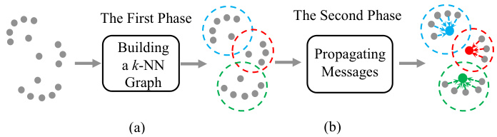
Figure 1. The pipeline of our approach. In the first phase (left), we build the $k{\mathrm{-NN}}$ graph, capturing the topology structure among data. For the second phase (right), we employ the GNN to aggregate features from high-confidence samples (nodes inside the dotted circle). The colored nodes represent the aggregated features.
图 1: 我们的方法流程。在第一阶段(左),我们构建 $k{\mathrm{-NN}}$ 图,捕捉数据间的拓扑结构。在第二阶段(右),我们使用 GNN 从高置信度样本(虚线圆圈内的节点)聚合特征。彩色节点表示聚合后的特征。
Construction of Graph. Formally, we denote $X_{q},X_{g}$ and $X_{u}$ as original features of query set, gallery set and the union of query and gallery set, respectively. There are $n$ images in query and gallery set in total. Let $G=(\mathcal{V},\mathcal{E})$ denote the graph where $\mathcal{V}={v_{1},...,v_{n}}$ are the vertices and $\mathcal{E}\subseteq\mathcal{V}\times\mathcal{V}$ are the edges. Each image is a vertex on the graph and connected edges represent the similarity between vertices.
图的构建。形式上,我们将 $X_{q},X_{g}$ 和 $X_{u}$ 分别表示为查询集、图库集以及查询集与图库集并集的原始特征。查询集和图库集中共有 $n$ 张图像。设 $G=(\mathcal{V},\mathcal{E})$ 表示图,其中 $\mathcal{V}={v_{1},...,v_{n}}$ 为顶点,$\mathcal{E}\subseteq\mathcal{V}\times\mathcal{V}$ 为边。每张图像作为图中的一个顶点,相连的边表示顶点之间的相似性。
First of all, cosine similarity matrix $\pmb{S}$ is calculated:
首先,计算余弦相似度矩阵 $\pmb{S}$:
$$
\begin{array}{l}{S_{i j}=c o s(x_{i},x_{j}),}\ {\mathrm{where}~x_{i},x_{j}\in X_{u},X_{u}=X_{q}\cup X_{g}.}\end{array}
$$
$$
\begin{array}{l}{S_{i j}=c o s(x_{i},x_{j}),}\ {\mathrm{where}~x_{i},x_{j}\in X_{u},X_{u}=X_{q}\cup X_{g}.}\end{array}
$$
Secondly, the features of neighbor relations are calculated. In $k$ -reciprocal re-ranking, [52] encode $k$ -reciprocal feature by selecting candidates from a expansion of $k$ -reciprocal neighbors. Masses of set intersection and comparison operations are required when selecting candidates, leading to huge time cost.
其次,计算邻居关系的特征。在$k$互逆重排序中,[52]通过从$k$互逆邻居的扩展中选择候选来编码$k$互逆特征。在选择候选时需要进行大量集合交集和比较操作,导致巨大的时间成本。
We overcome this drawback by adopting a simple but effective strategy to obtain the contextual information of the whole image group. Corresponding to the $k$ -reciprocal feature in re-ranking, we aim to encode node features by extracting neighbor information from $\pmb{S}$ on the entire graph.
我们通过采用一种简单而有效的策略来克服这一缺点,以获取整个图像组的上下文信息。对应于重排序中的 $k$-reciprocal 特征,我们的目标是通过从整个图的 $\pmb{S}$ 中提取邻居信息来编码节点特征。
where $\mathcal{N}(i,k_{1})$ is the $k_{1}$ most similar candidates according to similarity matrix $\pmb{S}$ . Generally, an ideal adjacent matrix should be symmetric. Further, the symmetric adjacent matrix $A^{*}$ is introduced as:
其中 $\mathcal{N}(i,k_{1})$ 是根据相似度矩阵 $\pmb{S}$ 得出的 $k_{1}$ 个最相似候选。理想情况下,邻接矩阵应具有对称性。因此引入对称邻接矩阵 $A^{*}$ 定义为:
$$
A^{*}=\frac{A+A^{T}}{2}.
$$
$$
A^{*}=\frac{A+A^{T}}{2}.
$$
We note that $A^{}$ encodes more adjacent information. It is because more neighbors are included and adaptive weights are assigned to high-confidence candidates. The experimental results in ablation study also show $A^{}$ performs better than $\pmb{A}$ . More importantly, due to the simplicity, symmetry and sparsity of $A^{}$ , the calculation process can be highly parallel iz able and efficient.
我们注意到 $A^{}$ 编码了更多相邻信息。这是因为包含了更多邻居节点,并为高置信度候选分配了自适应权重。消融研究中的实验结果也表明 $A^{}$ 的性能优于 $\pmb{A}$ 。更重要的是,由于 $ A^ $ 的简洁性、对称性和稀疏性,计算过程可以实现高度并行化且高效。
Here we define $h_{i}$ as the feature of vertex $v_{i}$ , which can be extracted from the $i$ -th row of the symmetric adjacent matrix $ A^{}$ :
这里我们将顶点 $v_{i}$ 的特征定义为 $h_{i}$ ,可从对称邻接矩阵 $A^{}$ 的第 $i$ 行提取:
$$
h_{i}=[A_{i,0}^{},...,A_{i,n}^{*}].
$$
$$
h_{i}=[A_{i,0}^{},...,A_{i,n}^{*}].
$$
Such neighbor encoding feature performs better than the original feature because the hard negative images usually share one different neighbor set with the true-matches. Hence we construct node features based on neighbor similarity rather than directly adopting the original features. The comparison between different features can be found in the ablation study.
这种邻居编码特征比原始特征表现更优,因为硬负样本图像通常与真实匹配项共享一组不同的邻居集合。因此我们基于邻居相似性构建节点特征,而非直接采用原始特征。不同特征的对比实验详见消融研究部分。
Finally, we build a $k$ -NN graph by connecting highconfidence edges to aggregate the feature of neighbors. Top $k_{2}$ edges in $S$ for each vertex are connected and the weights of edges are defined as:
最后,我们通过连接高置信度边来构建一个$k$-NN图,以聚合邻居特征。为每个顶点连接矩阵$S$中前$k_{2}$条边,边的权重定义为:
$$
e_{i j}=S_{i,j},j\in\mathcal{N}(i,k_{2}).
$$
$$
e_{i j}=S_{i,j},j\in\mathcal{N}(i,k_{2}).
$$
Message Propagation. In the second phase, a feature aggregating process is required to further improve the retrieval performance, which is achieved by a local query expansion in conventional re-ranking methods. Similarly, in our GNN formulation, this process can be achieved by the message propagating approach [9] on the graph. The key formula of this approach is described as below:
消息传播。在第二阶段,需要通过特征聚合过程进一步提升检索性能,这在传统重排序方法中通过局部查询扩展实现。类似地,在我们的GNN框架中,这一过程可通过图上的消息传播方法[9]完成。该方法的核心公式如下:
$$
h_{i}^{(l+1)}=h_{i}^{(l)}+a g g r e g a t e({f_{\Theta}(e_{i j})\cdot h_{j}^{(l)}}),
$$
$$
h_{i}^{(l+1)}=h_{i}^{(l)}+a g g r e g a t e({f_{\Theta}(e_{i j})\cdot h_{j}^{(l)}}),
$$
where hi(l) represents the feature of $v_{i}$ in the $l$ -th layer, $f_{\Theta}$ is the function to compute the weight of propagating message and aggregate represents the aggregator types: sum, mean or max.
其中 $h_{i}^{(l)}$ 表示第 $l$ 层中节点 $v_{i}$ 的特征,$f_{\Theta}$ 是计算传播消息权重的函数,aggregate 表示聚合器类型:求和 (sum)、平均 (mean) 或最大值 (max)。
We expect to find a suitable function $f_{\Theta}$ , which can capture the relation between nodes by edge weights. With message propagation, high-confidence node features are enhanced and the unreliable node features are weakened. Inspired by $\alpha$ -weighted query expansion $(\alpha{\mathrm{-QE}})$ [29], we adopt $f_{\Theta}(e_{i j})=e_{i j}^{\alpha}$ , where $\alpha$ is a fixed value. Then the formula of our modified GNN can be refined as below:
我们期望找到一个合适的函数 $f_{\Theta}$,它能够通过边权重捕捉节点间的关系。通过消息传播,高置信度的节点特征得到增强,而不可靠的节点特征被削弱。受 $\alpha$ 加权查询扩展 ($\alpha{\mathrm{-QE}}$) [29] 的启发,我们采用 $f_{\Theta}(e_{i j})=e_{i j}^{\alpha}$,其中 $\alpha$ 为固定值。于是改进后的 GNN 公式可简化为:
$$
h_{i}^{(l+1)}=h_{i}^{(l)}+a g g r e g a t e({e_{i j}^{\alpha}\cdot h_{j}^{(l)},j\in\mathcal{N}(i,k_{2})}).
$$
$$
h_{i}^{(l+1)}=h_{i}^{(l)}+a g g r e g a t e({e_{i j}^{\alpha}\cdot h_{j}^{(l)},j\in\mathcal{N}(i,k_{2})}).
$$
Besides, $h_{i}^{(l)}$ is regularized with $L_{2}$ norm after every message propagation on the graph. The last GNN layer will output the transformed node features $h_{i}^{(l)}$ . Finally, we derive the final ranking list according to the cosine similarity of refined features. Since the high-parallelism GNN propagates the message on the sparse graph efficiently, we can update all vertex features simultaneously. The whole algorithm is summarized in Algorithm 1.
此外,$h_{i}^{(l)}$ 在图上每次消息传播后都会用 $L_{2}$ 范数进行正则化。最后一层 GNN 将输出变换后的节点特征 $h_{i}^{(l)}$。最终,我们根据精炼特征的余弦相似度生成最终排序列表。由于高并行度的 GNN 能在稀疏图上高效传播消息,我们可以同时更新所有顶点特征。整个算法总结如算法 1 所示。
算法 1: 我们的方法框架。
| 输入: 查询和图库特征的并集 Xu; 超参数 k1 和 k2 |
3.4. Relation to Existing Methods
3.4. 与现有方法的关系
Our approach is related to two classes of approaches, reranking and GNN. The $k$ -reciprocal re-ranking [52] can be viewed as a special case of our approach. We argue that the first phase equals to building the neighbor graph, while the second phase can be viewed as spreading message within the graph.
我们的方法与两类方法相关:重排序和GNN (Graph Neural Network)。$k$-reciprocal重排序 [52] 可视为我们方法的一个特例。我们认为第一阶段等同于构建邻居图,而第二阶段可视为在图中传播消息。
In the first phase, the $k$ -reciprocal feature is essential to calculate Jaccard distance in conventional re-ranking. However, the $k$ -reciprocal feature requires to select the $k$ - reciprocal neighbors of query as candidates, and then expand the candidates set by adding the common neighbors of query and candidates. The set comparison operations are not hardware acceleration friendly. It is due to the crosscheck operation and a different number of $k$ -reciprocal candidates during expanding the neighbor sets. In contrast, our method performs relation modeling by building a $k\mathbf{\cdot}$ - NN graph. It is natural to implement by matrix operations, which can be deployed on GPU easily.
在第一阶段,$k$-reciprocal特征对于计算传统重排序中的Jaccard距离至关重要。然而,$k$-reciprocal特征需要选择查询的$k$-reciprocal邻居作为候选,然后通过添加查询与候选的共同邻居来扩展候选集。这种集合比较操作不利于硬件加速,原因在于交叉检查操作以及在扩展邻居集时$k$-reciprocal候选数量的差异。相比之下,我们的方法通过构建$k\mathbf{\cdot}$-NN图进行关系建模,这天然适合通过矩阵运算实现,可以轻松部署在GPU上。
In the second phase, local query expansion equals to one layer GNN with $\alpha=0$ (in Eq. 14) and the aggregator type sets to mean. The conventional query expansion message spreads with equal weights in a local region. In contrast, our approach spreads node features along with edge weights, combining both global and local information. We also enable different aggregate functions. In addition, as shown in experiments, the features of nodes can be further improved by aggregating features with the number of layers (i.e., twolayer GNN) increasing.
在第二阶段,局部查询扩展等同于一层 GNN (在公式 14 中设 $\alpha=0$ ),且聚合器类型设置为均值。传统查询扩展消息在局部区域内以等权重传播,而我们的方法则结合全局和局部信息,沿着边权重传播节点特征。我们还支持不同的聚合函数。此外,如实验所示,通过增加层数 (即两层 GNN) 聚合特征,可以进一步提升节点特征。
4. Experiment
4. 实验
We conduct experiments on five image retrieval datasets of different application scenarios, including a person reidentification dataset Market-1501 [47], a vehicle reidentification dataset VeRi-776 [21], two popular landmark retrieval datasets, i.e., Oxford $5\mathrm{k\Omega}$ [26] and Paris-6k [27], and a drone-based geo-localization dataset University1652 [49]. More details can be found in Section 4.1. Besides, we provide an ablation study about the effect of different components, GNN layer number and hyperparameters in Section 4.2. Finally, we discuss the retrieval results on five datasets in Section 4.3.
我们在五个不同应用场景的图像检索数据集上进行实验,包括行人重识别数据集 Market-1501 [47]、车辆重识别数据集 VeRi-776 [21]、两个热门地标检索数据集 Oxford $5\mathrm{k\Omega}$ [26] 和 Paris-6k [27],以及基于无人机的地理定位数据集 University1652 [49]。更多细节详见第4.1节。此外,我们在第4.2节提供了关于不同组件、GNN层数和超参数影响的消融研究。最后,我们在第4.3节讨论了五个数据集的检索结果。
4.1. Datasets and Settings
4.1. 数据集和设置
Market-1501. Market-1501 [47] is collected in front of a supermarket in Tsinghua University by six cameras. It contains 32,668 images of 1,501 identities in total. Specifically, it consists of 12,936 training images with 751 identities and 19,732 testing images with 750 identities. 3,368 images in the test set are selected as the query set. The images are detected by the DPM detector [8].
Market-1501。Market-1501 [47] 数据集由清华大学超市前的6个摄像头采集,共包含1,501个身份的32,668张图像。具体而言,该数据集包含751个身份的12,936张训练图像和750个身份的19,732张测试图像。测试集中有3,368张图像被选作查询集,所有图像均通过DPM检测器 [8] 进行检测。
VeRi-776. VeRi-776 [21] is collected in a real-world unconstrained traffic scene with various attribute annotations. Specifically, it contains 49,360 vehicle images of 776 vehicles captured by 20 cameras. 37,781 images of 576 vehicles are divided into the train set while 11,579 images of 200 vehicles are employed as the test set. The query set consists of 1,678 images.
VeRi-776. VeRi-776 [21] 数据集采集自真实无约束交通场景,包含多种属性标注。具体而言,该数据集包含20个摄像头拍摄的776辆车辆共49,360张图像。其中37,781张图像(576辆车辆)划分为训练集,11,579张图像(200辆车辆)作为测试集。查询集由1,678张图像组成。
Oxford $\mathbf{5k}$ . Oxford $\it{5k}$ [26] is one of the widely-used landmark retrieval datasets. It contains 5,062 images collected from Flickr by searching particular Oxford landmark names. The collected images are manually annotated for 11 different landmarks. There are 55 query images, and the rest images are leverages as the gallery.
Oxford $\mathbf{5k}$。Oxford $\it{5k}$ [26] 是广泛使用的地标检索数据集之一。它包含通过搜索特定牛津地标名称从Flickr收集的5,062张图像。收集的图像针对11个不同地标进行了人工标注,其中55张为查询图像,其余图像用作检索库。
Paris-6k. Similarly, Paris-6k [27] consists of 6,412 high resolution $(1024\times768)$ images collected from Flickr by searching particular Paris landmark names. There are 12 images in the query set.
Paris-6k。同样地,Paris-6k [27] 包含从Flickr通过搜索特定巴黎地标名称收集的6,412张高分辨率 $(1024\times768)$ 图像。查询集中有12张图像。
University-1652. University-1652 [49] contains 1,652 buildings of 72 universities around the world. There are 701 buildings of 33 universities in the training set, 701 buildings of the rest 39 universities in the test set, and 250 extra buildings serving as distract or s in the gallery set. In particular, there are 37,855 drone-based images in the query set, and 951 satellite-based images in the gallery set.
University-1652。University-1652 [49] 包含全球72所大学的1,652栋建筑。训练集包含33所大学的701栋建筑,测试集包含其余39所大学的701栋建筑,图库集则额外包含250栋干扰建筑。具体而言,查询集包含37,855张无人机拍摄图像,图库集包含951张卫星拍摄图像。
Evaluation Metrics. We mainly use mean average precision (mAP) [47] to evaluate the performance. For each query, the average precision (AP) is calculated according to the area under the Precision-Recall curve. Then we calculate the mean value of APs of all queries, i.e.,mAP, which takes both the precision and recall rate into consideration. The Recall $\ @\mathrm{K}$ [44, 20, 38] denotes whether the top
评估指标。我们主要使用平均精度均值 (mAP) [47] 来评估性能。对于每个查询,平均精度 (AP) 是根据精确率-召回率曲线下的面积计算的。然后我们计算所有查询 AP 的平均值,即 mAP,它同时考虑了精确率和召回率。召回率 $\ @\mathrm{K}$ [44, 20, 38] 表示是否在排名前 K 的结果中。
$K$ images contain a true match. The value of Recall $\ @\mathrm{K}$ equals to 1 if the first matched image has appeared before the $K$ -th image, which is sensitive to the position of the first matched image. On Market-1501 and VeRi-776, we also report the mean Recall $@1$ accuracy of all query images. For University-1652, according to the previous work [44, 20, 38], we add the Recall $@1$ , Recall $\ @5$ and Recall $@10$ of the retrieval results.
前 $K$ 张图像中包含真实匹配项。若首个匹配图像出现在第 $K$ 张图像之前,则召回率 $\ @\mathrm{K}$ 值为1,该指标对首个匹配图像的位置敏感。在Market-1501和VeRi-776数据集上,我们还报告了所有查询图像的平均召回率 $@1$ 准确率。对于University-1652数据集,根据先前工作 [20, 44, 38] 的设定,我们额外统计检索结果的召回率 $@1$、召回率 $\ @5$ 和召回率 $@10$。
Implementation Details. When testing, we use a two-layer GNN and set the aggregator as sum function. The parameter $\alpha$ in Eq. 14 is fixed as 2. For a fair comparison, we adopt the open-source baseline models to verify the effectiveness of the proposed method. In particular, we employ a popular open-source person re-identification networks2 as the Market-1501 baseline, which adopts a strong backbone, i.e., ResNet-50-ibn [23], and fuses multi-branch information to enhance the feature representation. The final feature dimension is 1536. For VeRi-776, we deploy a vehicle reidentification model3, which extracts the 2048-dimension feature. For Oxford $\it{5k}$ and Paris-6k, we similarly extract 2048-dimension visual feature from the open-source ResNet101-GeM4 [29] as the baseline. For University1652, we follow the official implementation of [49] as the baseline model5 and extract 512-dim visual feature. We note that all experiments are conducted on the same machine with one Intel(R) Xeon(R) CPU E5-2620 v2 $@$ 2.10Ghz, 164GB memory and one $\mathrm{K40m}$ GPU with 12GB memory.
实现细节。在测试时,我们使用两层GNN并将聚合器设置为求和函数。公式14中的参数$\alpha$固定为2。为确保公平比较,我们采用开源基线模型来验证所提方法的有效性。具体而言,我们采用一个流行的开源行人重识别网络2作为Market-1501的基线,该网络使用强大的骨干网络ResNet-50-ibn [23],并通过融合多分支信息来增强特征表示。最终特征维度为1536。对于VeRi-776,我们部署了一个车辆重识别模型3,提取2048维特征。对于Oxford $\it{5k}$和Paris-6k,我们同样从开源ResNet101-GeM4 [29]中提取2048维视觉特征作为基线。对于University1652,我们遵循[49]的官方实现作为基线模型5,并提取512维视觉特征。需要注意的是,所有实验均在同一台机器上进行,配置为Intel(R) Xeon(R) CPU E5-2620 v2 $@$2.10Ghz、164GB内存和一块12GB显存的$\mathrm{K40m}$ GPU。
4.2. Ablation Studies
4.2. 消融实验
Table 1. Ablation study. We study different feature inputs, i.e., original feature $x_{i}$ , adjacent matrix feature $\mathbf{}A_{i}$ and symmetric adjacent matrix feature $\boldsymbol{A}_{i}^{*}$ . Message propagation means aggregating the feature of neighbor nodes by Eq 13. Edge weights represent the weights of propagating message in $\mathrm{Eq}14$ . Two-layer GNN denotes the number of layers is 2.
表 1: 消融实验。我们研究了不同的特征输入,即原始特征 $x_{i}$、邻接矩阵特征 $\mathbf{}A_{i}$ 和对称邻接矩阵特征 $\boldsymbol{A}_{i}^{*}$。消息传播指通过公式13聚合邻居节点的特征。边权重表示公式14中消息传播的权重。双层GNN表示层数为2。
| 组件 | 性能 |
|---|---|
| 节点特征 $C_i$ 节点特征 $(A_i)$ 节点特征 $A$ 消息传播 边权重 | |
| 双层GNN mAP (%) Recall@1 (%) |
Effect of the GNN Layer Number. To take one step further, we study the impact of the different GNN layer numbers on the Market-1501 dataset. In Table 2, we report the Recall $@1$ and mAP with GNN from 1 layer to 256 layers. With the number of layers increasing, the node feature gradually moves to the mean value of the local connected neighbors, compromising the ranking performance. As a result, the Recall $@1$ reduces from $96.29%$ to $93.91%$ , and the mAP increases from $94.53%$ to $93.21%$ then reduces to $94.58%$ . As shown in Table 2, the mAP converges to $93.21%$ , when the number of the GNN layers is 256. In this case, the proposed method is approximately equal to the average query expansion (AQE) [6]. Because messages propagate again and again, yielding the over-smoothing result. In contrast, our method achieves the highest Recall $@1$ and mAP with one and two GNN layers.
GNN层数的影响。为进一步研究不同GNN层数对Market-1501数据集的影响,我们在表2中报告了从1层到256层GNN的Recall $@1$ 和mAP值。随着层数增加,节点特征逐渐趋近于局部连接邻居的平均值,导致排序性能下降。Recall $@1$ 从 $96.29%$ 降至 $93.91%$,mAP则从 $94.53%$ 升至 $93.21%$ 后回落至 $94.58%$。如表2所示,当GNN层数达到256层时,mAP收敛于 $93.21%$,此时所提方法近似等同于平均查询扩展(AQE)[6]。这是由于信息反复传播导致过度平滑现象。相比之下,我们的方法在1层和2层GNN时取得了最高的Recall $@1$ 和mAP值。
Effect of Hyper-parameter. To analyze the impact of two hyper-parameters $k_{1}$ and $k_{2}$ ), we conduct experiments on Market-1501 and VeRi-776 datasets. The hyper-parameter $k_{1}$ is used to calculate the adjacent matrix $A^{*}$ , while $k_{2}$ is the number of neighbors in message passing. Increasing the value of $k_{1}$ moderately introduces more neighbors. $k_{2}$ is much smaller than $k_{1}$ because a large value may bring noisy nodes. According to the previous work [36], the average number of images per class can be empirically estimated by $\left[{\frac{n}{C}}\right]$ $C$ represents the number of classes, $[\cdot]$ indicates round down operation) and it is reasonable to construct neighbor relations based on this value, thus we set:
超参数影响分析。为探究两个超参数 $k_{1}$ 和 $k_{2}$ 的影响,我们在 Market-1501 和 VeRi-776 数据集上进行了实验。其中 $k_{1}$ 用于计算邻接矩阵 $A^{*}$,而 $k_{2}$ 表示消息传递中的邻居数量。适度增大 $k_{1}$ 值可引入更多邻居节点,$k_{2}$ 取值远小于 $k_{1}$ 以避免噪声节点干扰。根据文献 [36],每类平均图像数可通过 $\left[{\frac{n}{C}}\right]$ 进行经验估计($C$ 表示类别数,$[\cdot]$ 为向下取整运算),基于该值构建邻居关系具有合理性,因此我们设定:
$$
k_{1}=[\frac{n}{C}].
$$
$$
k_{1}=[\frac{n}{C}].
$$
$k_{2}$ is estimated by a much smaller number than $k_{1}$ because a large value may bring noisy nodes. This selection rule is used in all following experiments. We first study the effect of $k_{1}$ by fixing the value of $k_{2}$ . $k_{2}$ is set to 7 and 10 on Market-1501 and VeRi-776 respectively. As shown in Figure 2 (a), our approach is insensitive to $k_{1}$ in a wide range from 20 to 40 on Market-1501. For VeRi-776, the proposed method maintains a relatively high performance when $k_{1}$ changes from 50 to 70. To evaluate the influence of parameter $k_{2}$ , we fix $k_{1}$ to 26 and 60 on Market-1501 and VeRi776 separately. Figure 2 (b) shows the pro form ance of our approach is stable on Market-1501 when $k_{2}$ changes from 5 to 10. Similar results can be achieved on VeRi-776 when keeping $k_{1}$ as 60 on VeRi-776 and changing $k_{2}$ from 10 to 15. In general, the proposed method can achieve comparable results and is relatively robust to a large range of $k_{1}$ and $k_{2}$ .
$k_{2}$ 的估计值远小于 $k_{1}$,因为较大的值可能会引入噪声节点。该选择规则在所有后续实验中使用。我们首先通过固定 $k_{2}$ 的值来研究 $k_{1}$ 的影响。$k_{2}$ 在 Market-1501 和 VeRi-776 上分别设置为 7 和 10。如图 2 (a) 所示,在 Market-1501 上,当 $k_{1}$ 在 20 到 40 的广泛范围内变化时,我们的方法对其不敏感。对于 VeRi-776,当 $k_{1}$ 从 50 变化到 70 时,所提方法保持了相对较高的性能。为了评估参数 $k_{2}$ 的影响,我们分别在 Market-1501 和 VeRi-776 上将 $k_{1}$ 固定为 26 和 60。图 2 (b) 显示,当 $k_{2}$ 从 5 变化到 10 时,我们的方法在 Market-1501 上的性能保持稳定。在 VeRi-776 上保持 $k_{1}$ 为 60 并将 $k_{2}$ 从 10 变化到 15 时,也能获得类似的结果。总体而言,所提方法能够取得可比的结果,并且对较大范围的 $k_{1}$ 和 $k_{2}$ 值具有相对鲁棒性。
Table 2. Effect of the GNN Layer Number. Comparison with different number of GNN layers on the Market-1501 dataset. With the number of layers increasing, the mAP accuracy converges to $93.21%$ . In this case, the proposed method is approximately equal to the average query expansion (AQE) [6].
表 2: GNN层数的影响。在Market-1501数据集上不同GNN层数的比较。随着层数增加,mAP准确率收敛至 $93.21%$。此时所提方法近似等于平均查询扩展(AQE) [6]。
| 方法 | Market-1501 Recall@1 (%) | mAP(%) |
|---|---|---|
| ours (1 layer) | 96.29 | 94.53 |
| ours (2 layers) | 96.11 | 94.65 |
| ours (4 layers) | 95.49 | 94.58 |
| ours (8 layers) | 95.96 | 94.45 |
| ours (16 layers) | 95.21 | 94.18 |
| ours (32 layers) | 94.92 | 93.90 |
| ours (64 layers) | 95.01 | 93.67 |
| ours (128 layers) | 94.44 | |
| 93.91 | 93.33 | |
| ours (256 layers) | 93.21 | |
| AQE [6] | 95.64 | 93.33 |

Figure 2. The hyper-parameter analysis on $k_{1}$ and $k_{2}$ . We analyze hyper-parameters on Market-1501 and VeRi-776. For Market-1501, we, following the previous work [36], empirically fix $k_{2}=7$ in (a) to study $k_{1}$ , and fix $k_{1}=26$ in $(\mathbf{b})$ to study $k_{2}$ . Similarly, for VeRi-776, we fix $k_{2}=10$ in (a) and $k_{1}=60$ in (b) to study the impact of hyper-parameters.
图 2: 超参数 $k_{1}$ 和 $k_{2}$ 的分析。我们在Market-1501和VeRi-776数据集上进行超参数分析。对于Market-1501,遵循先前工作[36]的经验设定,(a)中固定 $k_{2}=7$ 以研究 $k_{1}$ 的影响,(b)中固定 $k_{1}=26$ 以研究 $k_{2}$ 的影响。类似地,对于VeRi-776数据集,(a)固定 $k_{2}=10$,(b)固定 $k_{1}=60$ 来分析超参数的影响。
Table 3. Two-phase running time. We provide the running time of each phase and compare the proposed GNN-based method with the $\mathrm{k}$ -reciprocal method. The one-layer GNN is used to make a comparison with $k$ -reciprocal re-ranking, and we finally employ the two-layer GNN to achieve better performance. We observe that our method performs better and is faster than $k$ -reciprocal re-ranking on CPU. We also report the time cost of our method operating on GPU with a high parallelism.
表 3: 两阶段运行时间。我们提供了每个阶段的运行时间,并将提出的基于 GNN (Graph Neural Network) 的方法与 $\mathrm{k}$-互惠 (k-reciprocal) 方法进行比较。使用单层 GNN 与 $k$-互惠重排序进行对比,最终采用双层 GNN 以获得更好的性能。我们观察到,在 CPU 上,我们的方法表现更好且比 $k$-互惠重排序更快。我们还报告了我们的方法在高并行度的 GPU 上运行的时间成本。
| 方法 | 平台 | 阶段1 | 阶段2 | 总时间 | Recall@1 (%) | mAP (%) |
|---|---|---|---|---|---|---|
| k-reciprocal[52] | CPU | 49.0s | 40.2s | 89.2s | 94.65 | 96.11 |
| ours (1 layer) | CPU | 1.2s | 29.4s | 30.6s | 96.29 | 94.53 |
| ours (2 layers) | CPU | 1.2s | 58.7s | 59.9s | 96.11 | 94.65 |
| ours (2 layers) | GPU | 3.8ms | 5.6ms | 9.4ms | 96.11 | 94.65 |
Time Cost Comparison. We evaluate the efficiency of our method. We analyze the time cost of two phases on the Market-1501 dataset and compare our method with the conventional $k$ -reciprocal re-ranking. Here we adopt the official implementation 6. As shown in Table 3, we test the running time and performance of two methods on CPU. We can see that both the one-layer and two-layer GNN are faster than $k$ -reciprocal re-ranking in terms of the total time cost. To further reduce the time cost, we extend the GPUversion of our method, which can accelerate the re-ranking process to $\mathbf{9.4ms}$ . To the best of our knowledge, there is no available GPU implementation of $k$ -reciprocal re-ranking due to the sequential operations. Therefore, we do not include the GPU comparison with [52] but other methods [6] and [29]. As shown in Table 4 and Table 5, the proposed method finds one balance point between speed and performance. In general, our method achieves better performance on most datasets. In terms of the time cost on CPU, it is worth noting that proposed re-ranking method achieves the similar speed with SCA [1]. As for the GPU version, our method achieves a competitive speed with the vanilla methods including alpha-QE [29] and AQE [6], while we yield a better performance improvement.
时间成本对比。我们评估了所提方法的效率,在Market-1501数据集上分析两个阶段的时间消耗,并与传统$k$-reciprocal重排序方法进行对比。采用官方实现6进行测试。如表3所示,我们测量了两种方法在CPU上的运行时间和性能指标。实验表明,无论是单层还是双层GNN结构,其总耗时均快于$k$-reciprocal重排序。为进一步降低耗时,我们扩展了GPU版本实现,可将重排序过程加速至$\mathbf{9.4ms}$。由于$k$-reciprocal重排序存在顺序执行特性,目前尚无公开的GPU实现方案[52],因此表4和表5仅与[6][29]等方法进行GPU对比。实验结果表明,本方法在速度与性能之间取得了平衡:在多数数据集上获得更优性能表现;CPU耗时方面与SCA[1]速度相当;GPU版本在保持与alpha-QE[29]、AQE[6]等基础方法相当速度的同时,实现了更显著的性能提升。
4.3. Retrieval Performance
4.3. 检索性能
Experiments on Market-1501 and VeRi-776. As shown in Table 5, we compare the proposed method with other postprocessing approaches on the two re-identification dataset, i.e., Market-1501 and VeRi-776. There are two main observations. On the one hand, our method can improve mAP and Recall $@1$ by a large margin on the baseline. Specifically, our approach increases mAP by $6.39%$ and Recall $@1$ by $0.83%$ on Market-1501. On VeRi-776, we observe that the proposed approach gains $9.67%$ improvement on mAP and $0.83%$ improvement on the Recall $@1$ . On the other hand, we compare our approach with a variety of postprocessing methods, including two feature similarity-based methods: AQE [6], $\alpha$ -QE [29], two neighbor similar-based methods: SCA [1] and $k$ -reciprocal [52]. Results show that our approach outperforms all other methods both in mAP $(94.65%)$ and Recall $@1$ $(96.11%)$ on Market-1501. As for VeRi-776, our approach has achieved the highest mAP of $88.61%$ and second-best Recall $@1$ of $96.42%$ . Besides, we also compare the time cost of different post-processing methods both on CPU and GPU platforms in Table 4. The AQE [6] and $\alpha$ -QE [29] are implemented on GPU, while SCA [1] and $k$ -reciprocal re-ranking [52] operate on CPU due to the restriction of complex operations. The proposed method only takes about 9.4ms and ${\pmb{5.2m s}}$ to update Market-1501 and VeRi-776 respectively, which is significantly better than the traditional neighbor-based re-ranking method, and competitive to the method based on feature similarity.
在Market-1501和VeRi-776上的实验。如表5所示,我们在两个重识别数据集(Market-1501和VeRi-776)上将所提方法与其他后处理方法进行了对比。主要观察到两点:一方面,我们的方法能显著提升基线的mAP和Recall@1指标。具体而言,在Market-1501上mAP提升6.39%,Recall@1提升0.83%;在VeRi-776上mAP提升9.67%,Recall@1提升0.83%。另一方面,我们对比了包括两类后处理方法的结果:基于特征相似度的AQE [6]和α-QE [29],以及基于邻域相似度的SCA [1]和k-reciprocal [52]。实验表明,在Market-1501上我们的方法以mAP 94.65%和Recall@1 96.11%的表现优于所有对比方法;在VeRi-776上则取得了88.61%的最高mAP和96.42%的Recall@1(排名第二)。此外,表4对比了不同后处理方法在CPU和GPU平台上的耗时:AQE [6]和α-QE [29]在GPU运行,而SCA [1]和k-reciprocal重排序[52]因复杂运算限制只能在CPU运行。所提方法处理Market-1501和VeRi-776分别仅需约9.4ms和5.2ms,显著优于传统邻域重排序方法,与基于特征相似度的方法性能相当。
Table 4. Time cost. We compare the proposed method with various post-processing methods on Market-1501, VeRi-776, Oxford-5k, Paris6k and University-1652. We observe that our method finds one balance between speed and performance. For time cost on CPU, it is worth noting that proposed re-ranking method costs the same time as SCA. Besides, our method achieves a similar speed with alpha-QE [29] and AQE [6] but with large performance improvement on GPU.
表 4: 时间成本。我们在 Market-1501、VeRi-776、Oxford-5k、Paris6k 和 University-1652 数据集上将所提方法与多种后处理方法进行对比。观察到我们的方法在速度与性能之间找到了平衡点。值得注意的是,在 CPU 上运行时,所提重排序方法与 SCA 耗时相同。此外,我们的方法在 GPU 上实现了与 alpha-QE [29] 和 AQE [6] 相近的速度,同时带来显著的性能提升。
| 方法 | 平台 | Market-1501 | VeRi-776 | Oxford-5k | Paris-6k | University-1652 | 平均耗时 |
|---|---|---|---|---|---|---|---|
| AQE [6] | GPU | 3.4ms | 3.5ms | 1.8ms | 1.7ms | 8.3ms | 3.7ms |
| α-QE [29] | GPU | 3.6ms | 3.7ms | 1.9ms | 1.6ms | 9.1ms | 4.0ms |
| ours | GPU | 9.4ms | 5.2ms | 3.2ms | 3.5ms | 10.2ms | 6.3ms |
| SCA [1] | CPU | 43.2s | 18.4s | 25.6s | 25.6s | 89.7s | 40.5s |
| k-reciprocal [52] | CPU | 89.2s | 36.7s | 64.1s | 64.4s | 135.9s | 78.1s |
| ours | CPU | 60.0s | 21.3s | 17.1s | 23.2s | 85.5s | 41.4s |
Table 5. Retrieval performance. We compare the proposed method with various post-processing methods on Market-1501, VeRi-776, Oxford-5k, Paris-6k and University-1652. mAP $(%)$ means average precision. We observe that the proposed method achieves the best or second-best performance on most datasets.
表 5: 检索性能。我们在 Market-1501、VeRi-776、Oxford-5k、Paris-6k 和 University-1652 数据集上将所提方法与多种后处理方法进行比较。mAP (%) 表示平均精度。观察到所提方法在多数数据集上取得最优或次优性能。
| Methods | Market-1501 mAP (%) | Market-1501 Recall@1(%) | VeRi-776 mAP (%) | VeRi-776 Recall@1(%) | Oxford-5k mAP (%) | Paris-6k mAP (%) | University-1652 mAP(%) | University-1652 Recall@1(%) | University-1652 Recall@5(%) | University-1652 Recall@10(%) |
|---|---|---|---|---|---|---|---|---|---|---|
| baseline | 88.26 | 95.28 | 78.94 | 95.59 | 88.21 | 92.62 | 63.13 | 58.49 | 78.67 | 85.23 |
| AQE [5] | 93.33 | 95.64 | 82.49 | 89.22 | 90.63 | 96.04 | 71.23 | 67.62 | 83.32 | 86.36 |
| α-QE[29] | 93.51 | 96.08 | 82.77 | 89.72 | 91.07 | 95.45 | 71.69 | 68.18 | 83.66 | 86.71 |
| SCA [1] | 94.14 | 96.08 | 87.48 | 96.54 | 92.58 | 95.45 | 74.11 | 70.52 | 86.22 | 90.34 |
| k-reciprocal[52] | 94.38 | 95.90 | 88.44 | 96.36 | 92.31 | 96.49 | 73.67 | 70.71 | 83.86 | 85.65 |
| ours | 94.65 | 96.11 | 88.61 | 96.42 | 92.95 | 96.21 | 74.11 | 70.30 | 87.53 | 91.21 |
Experiments on Oxford-5k and Paris-6k. The proposed method is further evaluated on two small-scale landmark retrieval datasets, i.e., Oxford- $\it{5k}$ and Paris- $\mathrm{6k}$ . The performances of different post-processing methods on ResNet101-GeM [29] are reported in Table 5. The feature dimension is 2048. Our approach has achieved the highest mAP accuracy of $92.95%$ on Oxford- $\it{5k}$ , and compet- itive results $96.21%$ mAP accuracy on Paris-6k. The experiment verifies the s cal ability of the method on smallscale datasets. As shown in Table 4, the re-ranking process only consumes ${\pmb{5.2m s}}$ , which is faster than other re-ranking methods, i.e., SCA and $\mathbf{k}$ -reciprocal, and achieves a similar speed with the vanilla query expansion methods.
在Oxford-5k和Paris-6k上的实验。该方法进一步在两个小规模地标检索数据集(即Oxford-$\it{5k}$和Paris-$\mathrm{6k}$)上进行了评估。表5展示了不同后处理方法在ResNet101-GeM [29]上的性能表现,特征维度为2048。我们的方法在Oxford-$\it{5k}$上取得了92.95%的最高mAP准确率,在Paris-6k上也获得了具有竞争力的96.21% mAP准确率。实验验证了该方法在小规模数据集上的可扩展性。如表4所示,重排序过程仅消耗${\pmb{5.2m s}}$,比其他重排序方法(如SCA和$\mathbf{k}$-reciprocal)更快,且与原始查询扩展方法的速度相当。
Experiments on University-1652. We also provide experimental results on the drone-based geo-localization dataset [49]. Given one drone-view image, the droneview target localization task aims to find the corresponding satellite-view image to localize the target building in the satellite platform. From Table 5, we observe that our method can increase Recall $@1$ by $11.81%$ , Recall $\ @5$ by $8.86%$ , Recall $@10$ by $5.98%$ , and mAP by $10.98%$ . Comparing to other methods, our approach achieves the highest performance on Recall $\ @5$ , Recall $@10$ and mAP with $87.53%$ , $91.21%$ , and $74.11%$ respectively. From Table 4, we can see that the proposed method only consumes $\mathbf{10.2ms}$ on GPU and 85.5s on CPU.
University-1652上的实验。我们还提供了基于无人机的地理定位数据集[49]的实验结果。给定一张无人机视角图像,无人机视角目标定位任务旨在找到对应的卫星视角图像,以在卫星平台上定位目标建筑。从表5可以看出,我们的方法能将Recall $@1$ 提升 $11.81%$,Recall $@5$ 提升 $8.86%$,Recall $@10$ 提升 $5.98%$,mAP提升 $10.98%$。与其他方法相比,我们的方法在Recall $@5$、Recall $@10$和mAP上分别以 $87.53%$、$91.21%$ 和 $74.11%$ 取得了最高性能。从表4可以看出,所提方法在GPU上仅消耗 $\mathbf{10.2ms}$,在CPU上消耗85.5秒。
5. Conclusion
5. 结论
In this paper, we revisit re-ranking methods and identify the main challenge, i.e., high complexity. We re-formulate the re-ranking process as a graph neural network (GNN) function. Specifically, we explore the neighbor representation and deploy a two-layer GNN to aggregate the neighbor information of the entire data. The inherent attributes of GNN facilitate the parallel iz able implementation and make it a hardware-friendly acceleration approach. Extensive experiments on five datasets demonstrate that our method is competitive to existing arts in terms of both retrieval precision and running time. We hope this work can contribute to the future study of image retrieval tasks in real-world scenarios.
本文重新审视了重排序方法,并指出其主要挑战在于高复杂度问题。我们将重排序过程重新表述为图神经网络 (GNN) 函数,具体通过探索邻居表征并部署双层GNN来聚合整个数据的邻居信息。GNN的固有特性支持并行化实现,使其成为硬件友好的加速方案。在五个数据集上的大量实验表明,我们的方法在检索精度和运行时间方面均优于现有技术。希望这项工作能为现实场景中的图像检索任务研究提供有益参考。