HandOS: 3D Hand Reconstruction in One Stage
HandOS: 单阶段三维手部重建
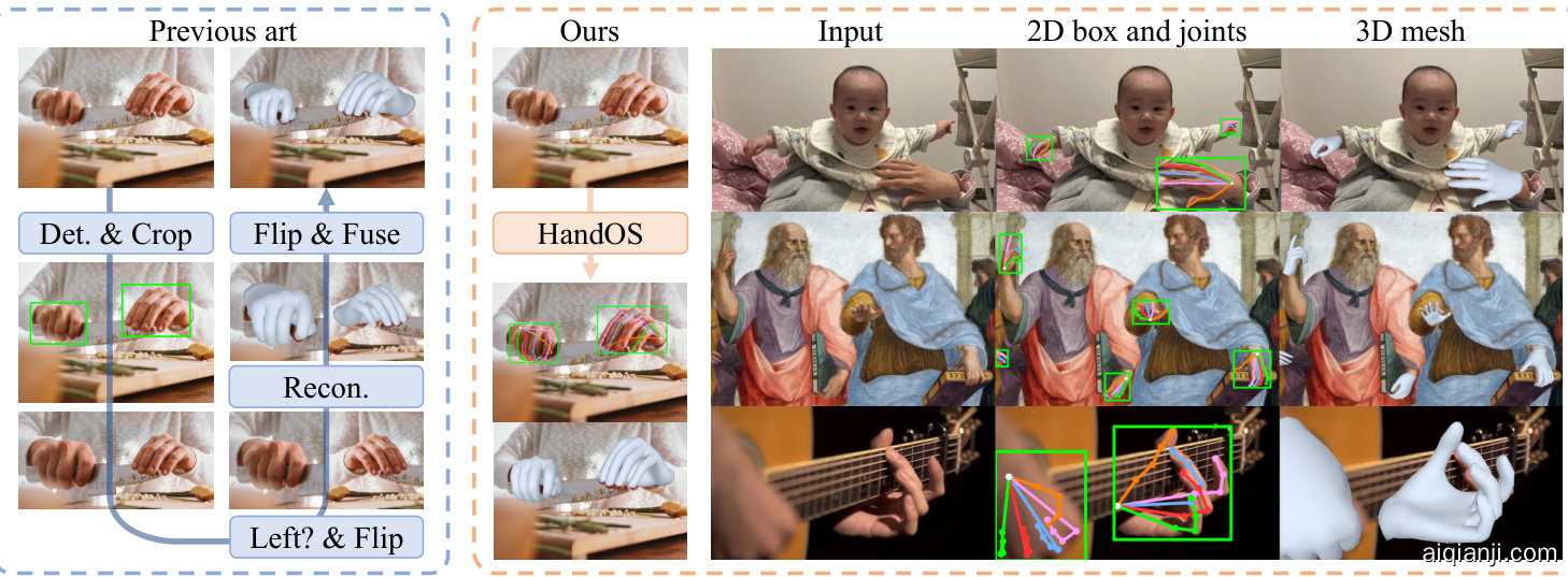
Figure 1. We present HandOS, a one-stage approach for hand reconstruction that substantially streamlines the paradigm. Additionally, we demonstrate that HandOS effectively adapts to diverse complex scenarios, making it highly applicable to real-world applications.
图 1: 我们提出了HandOS,这是一种用于手部重建的一阶段方法,大幅简化了现有范式。此外,我们证明了HandOS能有效适应各种复杂场景,使其在现实应用中具有高度适用性。
Abstract
摘要
Existing approaches of hand reconstruction predominantly adhere to a multi-stage framework, encompassing detection, left-right classification, and pose estimation. This paradigm induces redundant computation and cumulative errors. In this work, we propose HandOS, an end-to-end framework for 3D hand reconstruction. Our central motivation lies in leveraging a frozen detector as the foundation while incorporating auxiliary modules for 2D and 3D keypoint estimation. In this manner, we integrate the pose estimation capacity into the detection framework, while at the same time obviating the necessity of using the left-right category as a prerequisite. Specifically, we propose an interactive 2D-3D decoder, where 2D joint semantics is derived from detection cues while 3D representation is lifted from those of 2D joints. Furthermore, hierarchical attention is designed to enable the concurrent modeling of 2D joints, 3D vertices, and camera translation. Consequently, we achieve an end-to-end integration of hand detection, 2D pose estimation, and 3D mesh reconstruction within a one-stage framework, so that the above multi-stage drawbacks are overcome. Meanwhile, the HandOS reaches state-of-the-art performances on public benchmarks, e.g., 5.0 PA-MPJPE on FreiHand and 64.6% PCK@0.05 on HInt-Ego4D.
现有手部重建方法主要遵循多阶段框架,包括检测、左右手分类和姿态估计。这种范式会导致冗余计算和误差累积。本文提出HandOS——一个端到端的三维手部重建框架。我们的核心思路是以冻结检测器为基础,融入辅助模块进行2D和3D关键点估计。通过这种方式,我们将姿态估计能力整合到检测框架中,同时消除了左右手分类作为先决条件的必要性。具体而言,我们提出交互式2D-3D解码器:2D关节语义来自检测线索,3D表征则从2D关节提升而来。此外,设计了分层注意力机制来同步建模2D关节、3D顶点和相机位移。最终在单阶段框架内实现了手部检测、2D姿态估计和3D网格重建的端到端集成,从而克服了上述多阶段缺陷。HandOS在公开基准测试中达到最先进性能,例如FreiHand数据集上5.0的PA-MPJPE,HInt-Ego4D数据集上64.6%的PCK@0.05。
1. Introduction
1. 引言
The intellectual superiority of humans is expressed through their ability to use the hand to create, shape, and interact with the world. In the era of computer science and intelligence, hand understanding is crucial in reality technique [24, 57], behavior understanding [30, 46], interaction modeling [15, 69], embodied intelligence [11, 61], and etc.
人类智力的优越性体现在他们用手创造、塑造和与世界互动的能力上。在计算机科学与智能时代,手部理解在现实技术 [24, 57]、行为理解 [30, 46]、交互建模 [15, 69]、具身智能 [11, 61] 等领域至关重要。
Although hand mesh recovery has been studied for years, the pipeline is still confined to a multi-stage paradigm [2, 7, 8, 14, 36, 49], including detection, left-right recognition, and pose estimation. The necessities behind the multistage design are twofold. First, the hand typically occupies a limited resolution within an image, making the extraction of hand pose features from the entire image a formidable task. Hence, the detector is imperative to localize and upscale the hand regions. Second, the pose representation for the left and right hands exhibits symmetry rather than homogeneity [52]. Thus, a left-right recognizer is essential to flip the left hand to the right for a uniform pose representation. However, the multi-stage pipeline is computationally redundant, and the performance of pose estimation could be compromised by the dependencies on preceding results. For example, the error rate of detection and left-right classification reaches $11.2%$ , when testing ViTPose [65] on HInt test benchmark [49]. That is, some samples are determined to be incapable of yielding accurate results even before the pose estimation process. Therefore, we are inspired to overcome the above challenges by studying an end-to-end framework.
尽管手部网格恢复技术已研究多年,其流程仍局限于多阶段范式 [2, 7, 8, 14, 36, 49],包括检测、左右手识别和姿态估计。多阶段设计的必要性源于两方面:首先,手部在图像中通常仅占据有限分辨率,使得从整幅图像提取手部姿态特征成为艰巨任务,因此检测器必须定位并放大手部区域;其次,左右手的姿态表征呈现对称性而非同质性 [52],故需左右手识别器将左手翻转为右手以实现统一姿态表征。然而,多阶段流程存在计算冗余,且姿态估计性能易受前置结果依赖的影响。例如在HInt测试基准 [49] 上评估ViTPose [65] 时,检测与左右分类的错误率高达 $11.2%$,这意味着部分样本在姿态估计流程开始前即被判定无法产出准确结果。这促使我们研究端到端框架以攻克上述难题。
In this paper, we introduce a one-stage hand reconstruction model, termed HandOS, driven by two primary moti- vations. First, we utilize a pre-trained detector as the foundational model to derive the capacity of 3D reconstruction, with its parameters kept frozen during training. We choose to freeze the detector rather than simultaneously train the detection task because the approach to object detection is already well-studied, and this manner can facilitate data collection while also accelerating convergence. Moreover, to adapt the detector for our tasks, we employ a side-tuning strategy to generate adaptation features.
本文提出了一种单阶段手部重建模型HandOS,其设计基于两个核心动机。首先,我们采用预训练检测器作为基础模型来获取3D重建能力,并在训练期间保持其参数冻结。选择冻结检测器而非同步训练检测任务,是因为目标检测方法已得到充分研究,这种方式既能简化数据收集又能加速收敛。此外,为使检测器适配我们的任务,我们采用侧边调优策略来生成适应特征。
Second, we adopt a unified keypoint representation (i.e., 2D joints and 3D vertices) for both left and right hands, instead of MANO parameters. It is known that the hand usually occupies a small portion of an entire image, so we design an instance-to-joint query expansion to extract the semantics of 2D joints from the full image guided by detection results. Then, a question naturally arises – How to induce 3D semantics with 2D cues and perform 2D-3D information exchange? To this end, a 2D-to-3D query lifting is proposed to transform 2D queries into 3D space. Besides, considering the different properties between 2D and 3D elements, hierarchical attention is proposed for efficient training across 2D and 3D domains. Consequently, an interactive 2D-3D decoder is formed, capable of simultaneously modeling 2D joints, 3D vertices, and camera translation.
其次,我们采用统一的关键点表示方式(即2D关节和3D顶点)来处理左右手,而非MANO参数。由于手部通常在整幅图像中占据较小区域,因此我们设计了一种实例到关节的查询扩展机制,在检测结果引导下从全图中提取2D关节的语义信息。随之而来的问题是——如何利用2D线索推导3D语义并实现2D-3D信息交互?为此,我们提出2D到3D查询提升机制,将2D查询转换到3D空间。此外,考虑到2D与3D元素的不同特性,我们提出分层注意力机制以实现跨2D与3D领域的高效训练。最终构建的交互式2D-3D解码器能够同步建模2D关节、3D顶点和相机位移。
The contribution of this work lies in three-fold. (1) First of all, we propose an end-to-end HandOS framework for 3D hand reconstruction, where pose estimation is integrated into a frozen detector. Our one-stage superiority is also demonstrated by eliminating the need for prior classification of left and right hands. Therefore, the HandOS framework offers a streamlined architecture that is wellsuited for practical real-world applications. (2) We propose an interactive 2D-3D decoder with instance-to-joint query expansion, 2D-to-3D query lifting, and hierarchical attention, which allows for concurrent learning of 2D/3D keypoints and camera position. (3) The HandOS achieves superior performance in reconstruction accuracy via comprehensive evaluations and comparisons with state-of-the-art approaches, i.e., 5.0, 8.4, and 5.2 PA-MPJPE on FreiHand [81], HO3Dv3 [22], and DexYCB [6] benchmarks, along with $64.6%$ PCK $@0.05$ on HInt-Ego4D [49] benchmark.
本工作的贡献主要体现在三个方面:(1) 首先,我们提出了用于3D手部重建的端到端HandOS框架,将姿态估计集成到冻结检测器中。通过消除对左右手先验分类的需求,我们验证了单阶段架构的优越性。因此,HandOS框架提供了适合实际应用的简洁架构。(2) 我们提出了具有实例到关节查询扩展、2D到3D查询提升和分层注意力的交互式2D-3D解码器,可实现2D/3D关键点与相机位置的同步学习。(3) 通过综合评估与前沿方法的对比,HandOS在重建精度上展现出卓越性能:在FreiHand [81]、HO3Dv3 [22]和DexYCB [6]基准测试中分别达到5.0、8.4和5.2的PA-MPJPE,在HInt-Ego4D [49]基准测试中实现64.6%的PCK@0.05。
2. Related Work
2. 相关工作
3D hand reconstruction. Hand reconstruction approaches for monocular image can be broadly categorized into three types. The parametric method [1–4, 9, 25, 27, 38, 67, 69, 73, 75–78] typically employ MANO [52] as the parametric model and predicts the shape/pose coefficients to infer hand mesh. Voxel approaches [26, 44, 45, 68] utilize a 2.5D heatmap to represent 3D properties. Lastly, the vertex regression approach estimates the positions of vertices in 3D space [7, 8, 17, 33].
3D手部重建。针对单目图像的手部重建方法大致可分为三类。参数化方法 [1–4, 9, 25, 27, 38, 67, 69, 73, 75–78] 通常采用MANO [52] 作为参数化模型,通过预测形状/姿态系数来推断手部网格。体素方法 [26, 44, 45, 68] 使用2.5D热力图表示3D属性。最后,顶点回归方法直接估计3D空间中顶点的位置 [7, 8, 17, 33]。
Recently, the transformer technique [59] has been employed to enhance the performance [14, 31, 35, 36, 49, 71, 79]. Lin et al. [35] leveraged the transformer to develop a vertex regression framework, where a graph network is merged with the attention mechanism for structural understanding. Pavlakos et al. [49] utilized the transformer in a parametric framework. Thanks to the integration of $2.7\mathbf{M}$ training data, the generalization ability for in-the-wild images has been significantly enhanced. Dong et al. [14] also developed a transformer-like parametric framework with graph-guided Mamba [21], and a bidirectional Scan is proposed for shape-aware modeling. In our framework, we also incorporate the transformer architecture and develop an interactive 2D-3D decoder for learning keypoints in both 2D and 3D domains.
最近,Transformer技术[59]被用于提升性能[14, 31, 35, 36, 49, 71, 79]。Lin等人[35]利用Transformer开发了一个顶点回归框架,将图网络与注意力机制结合以实现结构理解。Pavlakos等人[49]在参数化框架中应用了Transformer。得益于整合的$2.7\mathbf{M}$训练数据,对自然场景图像的泛化能力得到了显著增强。Dong等人[14]也开发了一个类似Transformer的参数化框架,采用图引导的Mamba[21],并提出双向扫描(Scan)以实现形状感知建模。在我们的框架中,同样融入了Transformer架构,并开发了一个交互式2D-3D解码器,用于学习2D和3D领域的关键点。
All of the aforementioned methods adhere to a multistage paradigm, including detection and left-right recognition. The purpose of detection is to localize the hand and resize the hand region to a fixed resolution. Rather than utilizing an external detector, we directly enhance the pre-trained detector with the capability to perform pose estimation. Besides, our pipeline eliminates the need for resizing hand regions; instead, we employ instance-to-joint query expansion and deformable attention [80] to extract hand pose features effectively. The purpose of left-right recognition is to flip hand regions, standardizing the representation of left and right hands. In contrast, our approach eliminates the need for this stage, showing that left- and right-hand data can be jointly learned using our 2D-to-3D query lifting and hierarchical attention.
上述所有方法都遵循多阶段范式,包括检测和左右手识别。检测的目的是定位手部并将手部区域调整为固定分辨率。我们并非使用外部检测器,而是直接增强预训练检测器使其具备姿态估计能力。此外,我们的流程无需调整手部区域尺寸,转而采用实例到关节的查询扩展和可变形注意力 [80] 来高效提取手部姿态特征。左右手识别的目的是翻转手部区域以实现左右手的标准化表示。相比之下,我们的方法无需这一阶段,证明通过2D到3D查询提升和分层注意力机制可以联合学习左右手数据。

Figure 2. Overview of HandOS framework. Left: overall architecture. Right: interactive 2D-3D decoder. With off-the-shelf features, bounding boxes, and category scores from a frozen detector, the interactive 2D-3D decoder, including query filtering, expansion, lifting, and interactive layers, can understand hand pose and shape via estimating keypoints in both 2D and 3D spaces. Each query $\mathbf{Q}$ is associated with a reference box, which is not depicted in the figure for conciseness.
图 2: HandOS框架概览。左: 整体架构。右: 交互式2D-3D解码器。通过预训练检测器提供的现成特征、边界框和类别分数,包含查询过滤、扩展、提升和交互层的交互式2D-3D解码器,能够通过估计2D和3D空间中的关键点来理解手部姿态和形状。每个查询 $\mathbf{Q}$ 关联一个参考框(图中未示出以保持简洁)。
One-stage human pose estimation. With the advent of transformer-based object detection [5, 74], one-stage 2D pose estimation is advancing at a rapid pace. Shi et al. [54] proposed PETR, which is the first fully end-to-end pose estimation framework with hierarchical set prediction. Yang et al. [66] designed EDPose with human-to-keypoint decoder and interactive learning strategy to further enhance global and local feature aggregation.
单阶段人体姿态估计。随着基于Transformer的目标检测方法[5, 74]的出现,单阶段2D姿态估计正快速发展。Shi等人[54]提出了PETR框架,这是首个采用分层集合预测的完全端到端姿态估计方法。Yang等人[66]设计了EDPose,通过人体到关键点解码器和交互式学习策略进一步增强全局与局部特征聚合。
In the field of whole-body pose estimation, several works have focused on predicting SMPLX [48] parameters from monocular images in an end-to-end fashion. For example, Sun et al. [56] proposed AiOS, integrating whole-body detection and pose estimation in a coarse-to-fine manner. In contrast, our approach focuses on handling images that contain only hands in a one-stage framework. In addition, instead of utilizing parametric models, we use keypoints to align the representation of left and right hands, while also unifying the representations of 2D and 3D properties.
在全身体姿估计领域,多项研究致力于从单目图像端到端预测SMPLX[48]参数。例如,Sun等人[56]提出的AiOS通过粗到精的方式整合了全身检测与姿态估计。相比之下,我们的方法专注于在单阶段框架中处理仅包含手部的图像。此外,我们摒弃参数化模型,采用关键点对齐左右手表征,同时统一2D与3D属性的表征。
Two-hand reconstruction. Although approaches to interaction hands can simultaneously predict the pose of two hands [34, 43, 45, 50, 60, 72], they process left and right hands using separate modules and representations. Also, they need to classify the existence of the left and right. In contrast to related works that focus on modeling hand interactions, this paper focuses on single-hand reconstruction with a unified left-right representation.
双手重建。尽管交互手部的方法可以同时预测两只手的姿态 [34, 43, 45, 50, 60, 72],但它们使用独立的模块和表示分别处理左右手。此外,这些方法还需要对左右手的存在进行分类。与专注于手部交互建模的相关工作不同,本文重点研究采用统一左右手表示的单手重建。
3. Method
3. 方法
Given a single-view image $\mathbf{I}\in\mathbb{R}^{H\times W\times3}$ , we aim to infer a 2D joints $\mathbf{J}^{2D}\in\mathbb{R}^{J\times2}$ , 3D vertices ${\bf V}\in\mathbb{R}^{V\times3}$ , and camera translation $\mathbf{t}~\in\mathbb{R}^{3}$ , where $J=21,V=778$ . Then, 3D joints can be obtained from vertices, i.e., $\mathbf{J}^{3D}=\mathcal{I}\mathbf{V}$ , where $\mathcal{I}$ is the joint regressor defined by MANO [52]. With a fixed camera intrinsics $\mathbf{K}$ , 3D joints can be projected into image space, i.e., $\mathbf{J}^{p r o j}=\Pi_{\mathbf{K}}(\mathbf{J}^{3D}\mathbf{+}\mathbf{t})$ , where $\Pi$ is the projection function. The overall framework is shown in Fig. 2.
给定单视角图像 $\mathbf{I}\in\mathbb{R}^{H\times W\times3}$,我们的目标是推断出二维关节点 $\mathbf{J}^{2D}\in\mathbb{R}^{J\times2}$、三维顶点 ${\bf V}\in\mathbb{R}^{V\times3}$ 和相机平移量 $\mathbf{t}~\in\mathbb{R}^{3}$,其中 $J=21,V=778$。随后,三维关节点可通过顶点计算得出,即 $\mathbf{J}^{3D}=\mathcal{I}\mathbf{V}$,其中 $\mathcal{I}$ 是由 MANO [52] 定义的关节回归器。在固定相机内参 $\mathbf{K}$ 的情况下,三维关节点可投影至图像空间,即 $\mathbf{J}^{p r o j}=\Pi_{\mathbf{K}}(\mathbf{J}^{3D}\mathbf{+}\mathbf{t})$,其中 $\Pi$ 为投影函数。整体框架如图 2 所示。
3.1. Prerequisite: Grounding DINO
3.1. 前提条件:Grounding DINO
DETR-like detectors can serve as the foundation for HandOS. For instance, Grounding DINO [39] is utilized, which can detect objects with text prompts. In particular, we use “Hand” as the prompt without distinguishing the left and right. Referring to Fig. 2, Grounding DINO is a transformer-based architecture with a visual backbone $\boldsymbol{B^{v}}$ , a textual backbone $B^{t}$ , an encoder $\mathcal{E}$ , a decoder $\mathcal{D}$ , and a detection head $\mathcal{H}$ . The backbone [13, 16] takes images or texts as the input and produces features:
类似DETR的检测器可作为HandOS的基础。例如,我们采用Grounding DINO [39],该模型能够通过文本提示检测物体。具体而言,我们使用"Hand"作为提示词,且不区分左右手。如图2所示,Grounding DINO是基于Transformer的架构,包含视觉主干 $\boldsymbol{B^{v}}$、文本主干 $B^{t}$、编码器 $\mathcal{E}$、解码器 $\mathcal{D}$ 和检测头 $\mathcal{H}$。主干网络[13, 16]以图像或文本作为输入并生成特征:
$$
\begin{array}{r}{\mathcal{B}^{v}:\mathbf{I}\rightarrow\mathbf{F}^{v}\in\mathbb{R}^{L^{v}\times d^{v}},\quad\mathcal{B}^{t}:\mathbf{T}\rightarrow\mathbf{F}^{t}\in\mathbb{R}^{L^{t}\times d^{t}},}\end{array}
$$
$$
\begin{array}{r}{\mathcal{B}^{v}:\mathbf{I}\rightarrow\mathbf{F}^{v}\in\mathbb{R}^{L^{v}\times d^{v}},\quad\mathcal{B}^{t}:\mathbf{T}\rightarrow\mathbf{F}^{t}\in\mathbb{R}^{L^{t}\times d^{t}},}\end{array}
$$
where ${\bf F}^{v}$ represents a concatenated 4-scale feature with a flattened spatial resolution. $L^{v},L^{t}$ denote the length of the visual/textural tokens, and $d^{v},d^{t}$ are token dimensions.
其中 ${\bf F}^{v}$ 表示一个空间分辨率被展平的四尺度拼接特征。$L^{v},L^{t}$ 表示视觉/文本 token 的长度,$d^{v},d^{t}$ 为 token 的维度。
The encoder fuses and enhances features to generate a multi-modal representation with 6 encoding layers:
编码器通过融合和增强特征,生成具有6个编码层的多模态表示:
$$
\mathcal{E}:(\mathbf{F}^{v},\mathbf{F}^{t})\rightarrow\mathbf{F}^{e}\in\mathbb{R}^{T^{v}\times d^{v}}.
$$
$$
\mathcal{E}:(\mathbf{F}^{v},\mathbf{F}^{t})\rightarrow\mathbf{F}^{e}\in\mathbb{R}^{T^{v}\times d^{v}}.
$$
The decoder contains 6 decoding layers, aiming at extracting features from $\mathbf{F}^{e}$ with deformable attention and refining queries $\mathbf{Q}\in\mathbb{R}^{Q\times d^{q}}$ and reference boxes $\mathbf{R}\in\mathbb{R}^{Q\times4}$ , where $Q,d^{q}$ represent the number and dimension of queries. The decoding layer can be formulated as follows,
解码器包含6个解码层,旨在通过可变形注意力从$\mathbf{F}^{e}$中提取特征,并精炼查询$\mathbf{Q}\in\mathbb{R}^{Q\times d^{q}}$和参考框$\mathbf{R}\in\mathbb{R}^{Q\times4}$,其中$Q,d^{q}$分别表示查询的数量和维度。解码层可表述如下:
$$
\mathcal{D}:({\mathbf{Q}},{\mathbf{R}},{\mathbf{F}}^{e})\rightarrow{\mathbf{Q}},\quad{\mathbf{R}}=\mathrm{FFN}({\mathbf{Q}})+{\mathbf{R}},
$$
$$
\mathcal{D}:({\mathbf{Q}},{\mathbf{R}},{\mathbf{F}}^{e})\rightarrow{\mathbf{Q}},\quad{\mathbf{R}}=\mathrm{FFN}({\mathbf{Q}})+{\mathbf{R}},
$$
where FFN denotes feed forward network. Finally, the detection head predicts category scores and bounding boxes:
其中 FFN 表示前馈网络 (feed forward network)。最后,检测头预测类别分数和边界框:
$$
\begin{array}{r}{\mathcal{H}:(\mathbf{Q},\mathbf{R})\rightarrow(\mathbf{S},\mathbf{B})\in\mathbb{R}^{Q\times T^{t}}\times\mathbb{R}^{Q\times4}.}\end{array}
$$
$$
\begin{array}{r}{\mathcal{H}:(\mathbf{Q},\mathbf{R})\rightarrow(\mathbf{S},\mathbf{B})\in\mathbb{R}^{Q\times T^{t}}\times\mathbb{R}^{Q\times4}.}\end{array}
$$
As a result, we collect the output in each layer, obtaining an encoding feature set $\mathcal{F}^{e} =~{{\bf F}{i}^{e}}{i=1}^{6}$ , a query set $\mathcal{Q}={\mathbf{Q}{i}}_{i=0}^{6}$ . The index 0 indicates the initial elements before the decoder layers. Finally, the detection results are obtained from the last layer of detection head, producing the bounding box $\mathbf{B}$ and the corresponding score S.
因此,我们收集每一层的输出,获得编码特征集 $\mathcal{F}^{e} =~{{\bf F}{i}^{e}}{i=1}^{6}$ 、查询集 $\mathcal{Q}={\mathbf{Q}{i}}_{i=0}^{6}$ 。索引0表示解码器层之前的初始元素。最终,检测结果从检测头的最后一层获得,生成边界框 $\mathbf{B}$ 和对应分数S。
3.2. Side Tuning
3.2. 侧边调优 (Side Tuning)
To maintain off-the-shelf detection capability, we freeze all parameters in the detector. However, as the model is fully tamed for the detection task, keypoint-related representations in $\mathbf{F}^{e}$ remain insufficient. To conquer this difficulty, we design a learnable network with shadow layers of $\boldsymbol{B^{v}}$ as the input, generating complementary features $\mathbf{F}^{s}\in\mathbb{R}^{T^{v}\times d^{v}}$ . As a result, the Grounding DINO provides features, i.e., ${\bf F}^{G D}=[{\bf F}_{6}^{e},{\bf F}^{s}]$ , where $\left[\cdot,\cdot\right]$ denotes concatenation. Please refer to suppl. material for more details.
为了保持现成检测能力,我们冻结了检测器中所有参数。然而,由于模型已完全适配检测任务,$\mathbf{F}^{e}$ 中与关键点相关的表征仍然不足。为解决这一难题,我们设计了一个可学习网络,以 $\boldsymbol{B^{v}}$ 的阴影层作为输入,生成互补特征 $\mathbf{F}^{s}\in\mathbb{R}^{T^{v}\times d^{v}}$。最终,Grounding DINO 提供的特征表示为 ${\bf F}^{G D}=[{\bf F}_{6}^{e},{\bf F}^{s}]$,其中 $\left[\cdot,\cdot\right]$ 表示拼接操作。更多细节请参阅补充材料。
3.3. Interactive 2D-3D Decoder
3.3. 交互式 2D-3D 解码器
The input of decoder consists of $\mathbf{F}^{G D}$ , B, S, and queries $\mathbf{Q}^{i n s t}=\left[\mathbf{Q}{0},\mathbf{Q}_{6}\right]$ , while its output includes 2D joints $\mathbf{J}^{2D}$ , 3D vertices $\mathbf{V}$ , and camera translation $\mathbf{t}$ .
解码器的输入包括 $\mathbf{F}^{G D}$、B、S 和查询向量 $\mathbf{Q}^{i n s t}=\left[\mathbf{Q}{0},\mathbf{Q}_{6}\right]$,其输出则包含 2D 关节坐标 $\mathbf{J}^{2D}$、3D 顶点坐标 $\mathbf{V}$ 以及相机平移参数 $\mathbf{t}$。
Instance query filtering. Grounding DINO produces $Q$ instances but only a part of them belongs to the positive. During training, we employ SimOTA assigner [18] to assign instances to the positive based on ground truth. SimOTA first computes the pair-wise matching degree, which is represented by the cost $\mathbf{C}$ between the $i$ th prediction and the $j$ th ground truth (denoted by $\ '\star\ '$ ):
实例查询过滤。Grounding DINO 会生成 $Q$ 个实例,但其中只有一部分属于正样本。在训练过程中,我们采用 SimOTA 分配器 [18] 根据真实标注 (ground truth) 将实例分配为正样本。SimOTA 首先计算成对匹配度,用第 $i$ 个预测与第 $j$ 个真实标注 (表示为 $\ '\star\ '$ ) 之间的代价 $\mathbf{C}$ 来表示:
$$
\begin{array}{r l}&{{\bf{C}}{i,j}=-{\bf{S}}{j}^{\star}\log({\bf{S}}{i})-(1-{\bf{S}}{j}^{\star})\log(1-{\bf{S}}{i})}\ &{\quad\quad\quad-\log(\mathbb{I}\cup({\bf{B}}{i},{\bf{B}}_{j}^{\star})).}\end{array}
$$
$$
\begin{array}{r l}&{{\bf{C}}{i,j}=-{\bf{S}}{j}^{\star}\log({\bf{S}}{i})-(1-{\bf{S}}{j}^{\star})\log(1-{\bf{S}}{i})}\ &{\quad\quad\quad-\log(\mathbb{I}\cup({\bf{B}}{i},{\bf{B}}_{j}^{\star})).}\end{array}
$$
The cost function incorporates both classification error (i.e., binary cross-entropy) and localization error (i.e., Intersection over Union, IoU). Subsequently, an adaptive number $K$ is derived based on IoU, and top $K$ instances with the lowest cost are selected as the positive samples [19]. The selected queries and boxes are denoted as $\tilde{\mathbf{Q}}^{i n s t}\in\bar{\mathbb{R}}^{K\times d^{q}}$ and B E RKx4.
代价函数同时包含分类误差(即二元交叉熵)和定位误差(即交并比 IoU)。随后基于 IoU 推导出自适应数 $K$,并选择成本最低的前 $K$ 个实例作为正样本 [19]。所选查询和框表示为 $\tilde{\mathbf{Q}}^{i n s t}\in\bar{\mathbb{R}}^{K\times d^{q}}$ 和 B E RKx4。
In the inference phase, positive queries are identified by selecting those with a score threshold $T^{S}$ and a NMS threshold T NMS.
在推理阶段,通过选择分数阈值 $T^{S}$ 和非极大值抑制(NMS)阈值 T NMS 来识别正查询。
Instance-to-joint query expansion. We expand instance queries for 2D joint estimation. To this end, a learnable embedding ${\bf e}^{\bf Q}\in\mathbb{R}^{J\times d^{q}}$ is designed, and joint quires are obtained by adding $\mathbf{e^{Q}}$ with $\mathbf{Q}^{i n s t}$ :
实例到关节查询扩展。我们为2D关节估计扩展实例查询。为此,设计了一个可学习的嵌入 ${\bf e}^{\bf Q}\in\mathbb{R}^{J\times d^{q}}$ ,并通过将 $\mathbf{e^{Q}}$ 与 $\mathbf{Q}^{i n s t}$ 相加来获得关节查询:
$$
\mathbf{Q}^{\mathbf{J}^{2D}}\in\mathbb{R}^{K\times J\times d^{q}}=\tilde{\mathbf{Q}}^{i n s t}+\mathbf{e}^{\mathbf{Q}}.
$$
$$
\mathbf{Q}^{\mathbf{J}^{2D}}\in\mathbb{R}^{K\times J\times d^{q}}=\tilde{\mathbf{Q}}^{i n s t}+\mathbf{e}^{\mathbf{Q}}.
$$

Figure 3. Decoding layers. (a) Canonical 2D layer, popularly employed by previous works. (b) Interactive layer, where hierarchical attention is designed to effectively model 2D and 3D queries.
图 3: 解码层。(a) 经典2D层,被先前工作广泛采用。(b) 交互层,其中设计了分层注意力机制以有效建模2D和3D查询。
The reference boxes for 2D joints $\mathbf{R}^{\mathbf{J}^{2D}}\in\mathbb{R}^{K\times J\times4}$ can also be derived from instances following EDPose [66]:
2D关节的参考框 $\mathbf{R}^{\mathbf{J}^{2D}}\in\mathbb{R}^{K\times J\times4}$ 也可按照EDPose [66]的方法从实例中导出:
$$
\begin{array}{r l}{\mathbf{R}{c}^{\mathbf{J}^{2D}}\in\mathbb{R}^{K\times J\times2}=\mathrm{FFN}(\mathbf{Q}^{\mathbf{J}^{2D}})+\tilde{\mathbf{B}}{c},}\ {\mathbf{R}{s}^{\mathbf{J}^{2D}}\in\mathbb{R}^{K\times J\times2}=\tilde{\mathbf{B}}{s}\cdot\mathbf{e}_{2D}^{\mathbf{R}},}\end{array}
$$
$$
\begin{array}{r l}{\mathbf{R}{c}^{\mathbf{J}^{2D}}\in\mathbb{R}^{K\times J\times2}=\mathrm{FFN}(\mathbf{Q}^{\mathbf{J}^{2D}})+\tilde{\mathbf{B}}{c},}\ {\mathbf{R}{s}^{\mathbf{J}^{2D}}\in\mathbb{R}^{K\times J\times2}=\tilde{\mathbf{B}}{s}\cdot\mathbf{e}_{2D}^{\mathbf{R}},}\end{array}
$$
where the subscript $c,s$ represent the center and size of the reference box, and ${\bf e}_{2D}^{\bf R}\in\mathbb{R}^{J\times2}$ is the learnable embedding for the box size. FFN denotes feed forward network.
其中下标 $c,s$ 分别表示参考框的中心和大小,${\bf e}_{2D}^{\bf R}\in\mathbb{R}^{J\times2}$ 是框大小的可学习嵌入。FFN表示前馈网络。
2D-to-3D query lifting. Additionally, a third query transformation is employed, namely query lifting, wherein queries and reference boxes are elevated from 2D joints to 3D vertices and camera translation. To this end, we design a learnable lifting matrix $\mathbf{L}\in\mathbb{R}^{(V+1)\times J}$ as the weights for the linear combination between 2D and 3D queries, which is initialized with MANO skinning weights. Based on $\mathbf{L}$ , the lifting process can be formulated as
2D到3D查询提升。此外,还采用了第三种查询变换,即查询提升,将查询和参考框从2D关节点提升到3D顶点和相机平移。为此,我们设计了一个可学习的提升矩阵 $\mathbf{L}\in\mathbb{R}^{(V+1)\times J}$ 作为2D与3D查询之间线性组合的权重,该矩阵初始化为MANO蒙皮权重。基于 $\mathbf{L}$ ,提升过程可表述为
$$
\begin{array}{r l}{[{\mathbf{Q}^{\mathbf{V}}},{\mathbf{Q}^{\mathbf{t}}}]\in\mathbb{R}^{K\times(V+1)\times d^{q}}={\mathbf{L}}\diamond{\mathbf{Q}^{{\mathbf{J}}^{2D}}},}\ {[{\mathbf{R}^{\mathbf{V}}},{\mathbf{R}^{\mathbf{t}}}]\in\mathbb{R}^{K\times(V+1)\times4}={\mathbf{L}}\diamond{\mathbf{R}^{{\mathbf{J}}^{2D}}},}\ {[{\mathbf{R}{c}^{\mathbf{V}}},{\mathbf{R}{c}^{\mathbf{t}}}]=\mathrm{FFN}([{\mathbf{Q}^{\mathbf{V}}},{\mathbf{Q}^{\mathbf{t}}}])+[{\mathbf{R}{c}^{\mathbf{V}}},{\mathbf{R}{c}^{\mathbf{t}}}],}\ {[{\mathbf{R}{s}^{\mathbf{V}}},{\mathbf{R}{s}^{\mathbf{t}}}]=[{\mathbf{R}{s}^{\mathbf{V}}},{\mathbf{R}{s}^{\mathbf{t}}}]\cdot{\mathbf{e}_{3D}^{\mathbf{R}}},}\end{array}
$$
$$
\begin{array}{r l}{[{\mathbf{Q}^{\mathbf{V}}},{\mathbf{Q}^{\mathbf{t}}}]\in\mathbb{R}^{K\times(V+1)\times d^{q}}={\mathbf{L}}\diamond{\mathbf{Q}^{{\mathbf{J}}^{2D}}},}\ {[{\mathbf{R}^{\mathbf{V}}},{\mathbf{R}^{\mathbf{t}}}]\in\mathbb{R}^{K\times(V+1)\times4}={\mathbf{L}}\diamond{\mathbf{R}^{{\mathbf{J}}^{2D}}},}\ {[{\mathbf{R}{c}^{\mathbf{V}}},{\mathbf{R}{c}^{\mathbf{t}}}]=\mathrm{FFN}([{\mathbf{Q}^{\mathbf{V}}},{\mathbf{Q}^{\mathbf{t}}}])+[{\mathbf{R}{c}^{\mathbf{V}}},{\mathbf{R}{c}^{\mathbf{t}}}],}\ {[{\mathbf{R}{s}^{\mathbf{V}}},{\mathbf{R}{s}^{\mathbf{t}}}]=[{\mathbf{R}{s}^{\mathbf{V}}},{\mathbf{R}{s}^{\mathbf{t}}}]\cdot{\mathbf{e}_{3D}^{\mathbf{R}}},}\end{array}
$$
where $\mathbf{e}_{3D}^{\mathbf{R}}\in\mathbb{R}^{(V+1)\times2}$ is the embedding for the box size, and $\diamond$ denotes Einstein summation for linear combination.
其中 $\mathbf{e}_{3D}^{\mathbf{R}}\in\mathbb{R}^{(V+1)\times2}$ 是包围盒尺寸的嵌入表示,$\diamond$ 表示线性组合的Einstein求和约定。
Decoding layer and hierarchical attention. Referring to Fig. 2, the decoder comprises 6 layers, with the initial two being designated as 2D layers, and the remaining four functioning as interactive layers. The 2D layer contains selfattention, deformable attention [80], and FFN in Fig. 3(a).
解码层与层级注意力机制。如图 2 所示,解码器包含 6 层结构,其中前两层为 2D 层,后四层为交互层。2D 层包含图 3(a) 中的自注意力 (self-attention)、可变形注意力 [80] 和 FFN 模块。
However, the popular design of Fig. 3(a) cannot directly apply to interactive 2D-3D learning. This is caused by the different properties of 2D joints, 3D vertices, and camera translation: the 2D joints and 3D vertices should exhibit invariance to translation and scale, while the camera parameters should be sensitive for both translation and scale. That is, when the object appears in different positions and scales within the image, the relative structure of the 2D joints $\mathbf{J}^{2D}$ remains unchanged, the spatial coordinates of the 3D vertices $\mathbf{V}$ stay constant, while the 3D camera translation t varies. Hence, QJ2D and $\mathbf{Q}^{\mathbf{V}}$ should avoid performing attention operations with $\mathbf{Q^{t}}$ . Conversely, camera translation is significantly influenced by both 2D position and 3D geometry. Therefore, we enable $\mathbf{Q^{t}}$ to focus its attention on QJ2D and $\mathbf{Q}^{\mathbf{V}}$ . Furthermore, 3D vertices provide a robust representation of geometric structure, whereas 2D joints capture rich semantics of image features. Therefore, we allow them to attend to each other, serving as complementary features. We refer to this operation as hierarchical attention, through which an interactive layer is formulated as shown in Fig. 3(b). The arrows in hierarchical attention indicate the visibility of the attention mechanism, with the attention mask as shown in Fig. 8(c).
然而,图 3(a) 的流行设计无法直接应用于交互式 2D-3D 学习。这是由于 2D 关节点、3D 顶点和相机平移的不同特性所致:2D 关节点和 3D 顶点应表现出对平移和尺度变化的不变性,而相机参数则应对平移和尺度变化敏感。也就是说,当物体在图像中以不同位置和尺度出现时,2D 关节点 $\mathbf{J}^{2D}$ 的相对结构保持不变,3D 顶点 $\mathbf{V}$ 的空间坐标保持恒定,而 3D 相机平移 t 会发生变化。因此,QJ2D 和 $\mathbf{Q}^{\mathbf{V}}$ 应避免与 $\mathbf{Q^{t}}$ 进行注意力操作。相反,相机平移受 2D 位置和 3D 几何的显著影响。因此,我们让 $\mathbf{Q^{t}}$ 将其注意力集中在 QJ2D 和 $\mathbf{Q}^{\mathbf{V}}$ 上。此外,3D 顶点提供了几何结构的鲁棒表示,而 2D 关节点则捕获了图像特征的丰富语义。因此,我们允许它们相互关注,作为互补特征。我们将此操作称为分层注意力,通过该操作,交互层如图 3(b) 所示。分层注意力中的箭头表示注意力机制的可见性,注意力掩码如图 8(c) 所示。
Finally, we use FFN as heads for the regression of 2D joints, 3D vertices, and camera translation.
最后,我们使用 FFN 作为头部来回归 2D 关节、3D 顶点和相机平移。
3.4. Loss Functions
3.4. 损失函数
2D supervision. We use point-wise L1 error and object keypoints similarity (OKS) [42] as the criterion to produce loss terms from 2D annotation (denoted by $\mathbf{\hat{\Sigma}}^{66}\star\mathbf{\hat{\Sigma}}^{,}$ ):
2D监督。我们采用逐点L1误差和物体关键点相似度 (OKS) [42] 作为标准,从2D标注生成损失项(表示为 $\mathbf{\hat{\Sigma}}^{66}\star\mathbf{\hat{\Sigma}}^{,}$):
$$
\begin{array}{r l}&{\mathcal{L}^{\mathbf{J}^{2D}}=||\mathbf{J}^{2D}-\mathbf{J}^{2D\star}||{1},}\ &{\mathcal{L}_{O K S}^{2D}=\mathsf{O K S}(\mathbf{J}^{2D},\mathbf{J}^{2D\star}).}\end{array}
$$
$$
\begin{array}{r l}&{\mathcal{L}^{\mathbf{J}^{2D}}=||\mathbf{J}^{2D}-\mathbf{J}^{2D\star}||{1},}\ &{\mathcal{L}_{O K S}^{2D}=\mathsf{O K S}(\mathbf{J}^{2D},\mathbf{J}^{2D\star}).}\end{array}
$$
3D supervision. We use point-wise L1 error, edge-wise L1 error, and normal similarity to formulate 3D loss terms:
3D监督。我们使用逐点L1误差、边缘L1误差和法线相似度来构建3D损失项:
$$
\begin{array}{l}{\displaystyle\mathcal{L}^{\mathbf{V}}=||\mathbf{V}-\mathbf{V}^{\star}||{1},\quad\mathcal{L}^{\mathbf{J}^{3D}}=||\mathbf{J}^{3D}-\mathbf{J}^{3D}||{1},}\ {\displaystyle\mathcal{L}^{n o r m a l}=\sum_{\mathbf{f}\in\mathbb{F}}\sum_{(i,j)\subset\mathbf{f}}|\frac{\mathbf{V}{i}-\mathbf{V}{j}}{||\mathbf{V}{i}-\mathbf{V}{j}||{2}}\cdot\mathbf{n}{\mathbf{f}}^{\star}|,}\ {\displaystyle\mathcal{L}^{e d g e}=\sum_{\mathbf{f}\in\mathbb{F}}\sum_{(i,j)\subset\mathbf{f}}|||\mathbf{V}{i}-\mathbf{V}{j}||{2}-||\mathbf{V}{i}^{\star}-\mathbf{V}{j}^{\star}||_{2}|,}\end{array}
$$
$$
\begin{array}{l}{\displaystyle\mathcal{L}^{\mathbf{V}}=||\mathbf{V}-\mathbf{V}^{\star}||{1},\quad\mathcal{L}^{\mathbf{J}^{3D}}=||\mathbf{J}^{3D}-\mathbf{J}^{3D}||{1},}\ {\displaystyle\mathcal{L}^{n o r m a l}=\sum_{\mathbf{f}\in\mathbb{F}}\sum_{(i,j)\subset\mathbf{f}}|\frac{\mathbf{V}{i}-\mathbf{V}{j}}{||\mathbf{V}{i}-\mathbf{V}{j}||{2}}\cdot\mathbf{n}{\mathbf{f}}^{\star}|,}\ {\displaystyle\mathcal{L}^{e d g e}=\sum_{\mathbf{f}\in\mathbb{F}}\sum_{(i,j)\subset\mathbf{f}}|||\mathbf{V}{i}-\mathbf{V}{j}||{2}-||\mathbf{V}{i}^{\star}-\mathbf{V}{j}^{\star}||_{2}|,}\end{array}
$$
where $\mathbb{F}$ represents mesh faces defined by MANO [52]. Lnormal, Ledge are important in our pipeline to induce a rational geometry shape without the aid of MANO inference.
其中 $\mathbb{F}$ 表示由 MANO [52] 定义的网格面。Lnormal 和 Ledge 在我们的流程中至关重要,它们能在无需 MANO 推理的情况下引导出合理的几何形状。
Weak supervision. The majority of samples captured from daily life lack precise 3D annotations. To address this, we introduce weak loss terms based on normal consistency
弱监督。从日常生活中捕获的大多数样本缺乏精确的3D标注。为解决这一问题,我们引入了基于法线一致性的弱损失项

Figure 4. Normal vectors serve as left-right indicator. When applying right-hand faces to left or right vertices, the directions of the normal vectors are opposed, as illustrated by the purple lines.
图 4: 法向量作为左右指示器。当将右侧面应用于左侧或右侧顶点时,法向量的方向相反,如紫色线条所示。
and projection error, enabling the use of 2D annotations for hand mesh learning:
和投影误差,使得能够利用2D标注进行手部网格学习:
$$
\begin{array}{r l}{\mathcal{L}^{{\mathbf{J}^{p r o j}}}=||\mathbf{J}^{p r o j}-\mathbf{J}^{2D\star}||{1},}\ {\mathcal{L}{O K S}^{p r o j}=\mathrm{OKS}(\mathbf{J}^{p r o j},\mathbf{J}^{2D\star}),}\ {\mathcal{L}^{n c}=\sum_{\mathbf{n}{1},\mathbf{n}{2}}(1-<\mathbf{n}{1},\mathbf{n}_{2}>),}\end{array}
$$
$$
\begin{array}{r l}{\mathcal{L}^{{\mathbf{J}^{p r o j}}}=||\mathbf{J}^{p r o j}-\mathbf{J}^{2D\star}||{1},}\ {\mathcal{L}{O K S}^{p r o j}=\mathrm{OKS}(\mathbf{J}^{p r o j},\mathbf{J}^{2D\star}),}\ {\mathcal{L}^{n c}=\sum_{\mathbf{n}{1},\mathbf{n}{2}}(1-<\mathbf{n}{1},\mathbf{n}_{2}>),}\end{array}
$$
where $\mathbf{n}{1},\mathbf{n}_{2}$ are normals of neighboring faces with shared edge, and $<\cdot,\cdot>$ denotes inner product.
其中 $\mathbf{n}{1},\mathbf{n}_{2}$ 是共享边的相邻面法向量,$<\cdot,\cdot>$ 表示内积。
Overall, the total loss function is a weighted sum of the above terms, which is applied not only to the final results but also to the intermediate outputs.
总体而言,总损失函数是上述各项的加权和,不仅应用于最终结果,也应用于中间输出。
3.5. Normal Vector as Left-Right Indicator
3.5. 法向量作为左右指示器
The HandOS neither requires a left-right category as a prerequisite nor explicitly incorporates a left-right classification module. Nevertheless, the left-right information is al- ready embedded in the reconstructed mesh. Specifically, we use the normal vector as the indicator. As shown in Fig. 4, based on the right-hand face, if the mesh belongs to the left hand, the normal vectors point towards the geometric interior; otherwise, they point towards the geometric exterior. In this manner, the left-right category is obtained.
HandOS 既不需要以左右类别作为前提,也没有明确包含左右分类模块。然而,左右信息已经嵌入到重建的网格中。具体来说,我们使用法向量作为指示器。如图 4 所示,基于右手表面,如果网格属于左手,法向量指向几何内部;否则指向几何外部。通过这种方式即可获得左右类别。
4. Experiments
4. 实验
4.1. Implement Details
4.1. 实现细节
Datasets including FreiHand [81], HO3Dv3 [22], DexYCB [6], HInt [49], COCO-WholeBody [29], and Onehand10K [62] are employed for experiments. For the FreiHand, HO3Dv3, and DexYCB benchmarks, we utilize their respective training datasets. To evaluate the HInt benchmark, we aggregate the FreiHand, HInt, COCO-WholeBody, and Onehand10K datasets for training. This combined dataset provides 204K samples, forming a subset of the 2,749K training samples used by HaMeR [49].
实验采用了包括FreiHand [81]、HO3Dv3 [22]、DexYCB [6]、HInt [49]、COCO-WholeBody [29]和Onehand10K [62]在内的数据集。针对FreiHand、HO3Dv3和DexYCB基准测试,我们使用了它们各自的训练数据集。为评估HInt基准,我们整合了FreiHand、HInt、COCO-WholeBody和Onehand10K数据集进行训练。该组合数据集提供了204K样本,构成HaMeR [49]所用2,749K训练样本的子集。
We utilize Grounding DINO 1.5 [51] as the pre-trained detector to exemplify our approach, noting that our framework is adaptable to other DETR-like detectors. The input is a full image, rather than a cropped hand patch, with its long edge resized to 1280 pixels, following the configuration of Grounding DINO 1.5. We employ the Adam opti- mizer [32] to train our model over 40 epochs with a batch size of 16. The learning rate is initialized at 0.001, with a cosine decay applied from the 25th epoch onward. On the FreiHand dataset, model training takes approximately 6 days using 8 A100-80G GPUs.
我们采用 Grounding DINO 1.5 [51] 作为预训练检测器来示例我们的方法,并指出我们的框架可适配其他类 DETR 的检测器。输入为完整图像(而非裁剪的手部区域),按照 Grounding DINO 1.5 的配置将其长边调整为 1280 像素。我们使用 Adam 优化器 [32] 训练模型 40 个周期,批量大小为 16。初始学习率为 0.001,从第 25 个周期开始采用余弦衰减。在 FreiHand 数据集上,使用 8 块 A100-80G GPU 训练模型约需 6 天。
Table 1. Results on FreiHand. Errors are measured in mm.
| Method | PJ ↓ | PV ↓ F@5↑ | F@15↑ | |
| METRO [36] | 6.7 | 6.8 | 0.717 | 0.981 |
| MeshGraphormer [35] | 5.9 | 6.0 | 0.765 | 0.987 |
| MobRecon [8] | 5.7 | 5.8 | 0.784 | 0.986 |
| PointHMR[31] | 6.1 | 6.6 | 0.720 | 0.984 |
| Zhouetal.[79] | 5.7 | 6.0 | 0.772 | 0.986 |
| HaMeR[49] | 6.0 | 5.7 | 0.785 | 0.990 |
| Hamba [14] | 5.8 | 5.5 | 0.798 | 0.991 |
| HandOS (ours) | 5.0 | 5.3 | 0.812 | 0.991 |
表 1. FreiHand上的结果。误差以毫米为单位。
| 方法 | PJ ↓ | PV ↓ F@5↑ | F@15↑ |
|---|---|---|---|
| METRO [36] | 6.7 | 6.8 | 0.717 |
| MeshGraphormer [35] | 5.9 | 6.0 | 0.765 |
| MobRecon [8] | 5.7 | 5.8 | 0.784 |
| PointHMR [31] | 6.1 | 6.6 | 0.720 |
| Zhou et al. [79] | 5.7 | 6.0 | 0.772 |
| HaMeR [49] | 6.0 | 5.7 | 0.785 |
| Hamba [14] | 5.8 | 5.5 | 0.798 |
| HandOS (ours) | 5.0 | 5.3 | 0.812 |
Table 2. Results on FreiHand with left hands in training data.
| Image fip in training | ↑fd | PV← | F@5↑ | F@15↑ |
| 5.0 | 5.3 | 0.812 | 0.991 | |
| √ | 5.3 | 5.6 | 0.799 | 0.989 |
表 2: 训练数据中包含左手的FreiHand结果
| 训练中图像翻转 | ↑fd | PV← | F@5↑ | F@15↑ |
|---|---|---|---|---|
| 5.0 | 5.3 | 0.812 | 0.991 | |
| √ | 5.3 | 5.6 | 0.799 | 0.989 |
PA-MPJPE (abbreviated as PJ), PA-MPVPE (abbreviated as PV), F-socre, PCK, and AUC are used as metrics for evaluation [8, 49] with $T^{S}=0.1,T^{N M S}=0.9$ .
PA-MPJPE (缩写为PJ)、PA-MPVPE (缩写为PV)、F-score、PCK和AUC被用作评估指标 [8, 49],其中 $T^{S}=0.1,T^{N M S}=0.9$。
4.2. Main Results
4.2. 主要结果
We use Green and Light Green to indicate the best and second results. Previous methods assume that detection and left-right category are accurate, only measuring mesh reconstruction error. In contrast, we do not use the perfect assumption, and our detector achieves 0.44 box AP when measuring hand [29] on COCO val2017 [37]. In terms of missed detection, we use $\mathbf{V}=\mathbf{0}$ for 3D metrics and set 0 for PCK/AUC. Hence, our results reflect mixed errors across detection, left-right awareness, and mesh reconstruction.
我们使用绿色和浅绿色分别表示最佳和次佳结果。先前的方法假设检测和左右类别判断是准确的,仅测量网格重建误差。相比之下,我们未采用完美假设,当在COCO val2017 [37]上测量手部检测时,我们的检测器实现了0.44的边界框AP [29]。对于漏检情况,我们使用$\mathbf{V}=\mathbf{0}$计算3D指标,并将PCK/AUC设为0。因此,我们的结果反映了检测、左右感知和网格重建的混合误差。
FreiHand. As shown in Table 1, the HandOS demonstrates a notable advantage over prior arts in reconstruction accuracy. Since FreiHand contains only right-hand samples, we flip images to generate left-hand samples for training. According to Table 2, we provide a unified left-right representation and support simultaneous learning for both left and right hands, delivering results comparable to those achieved with right-only training.
FreiHand。如表 1 所示,HandOS 在重建精度上展现出显著优于现有技术的优势。由于 FreiHand 仅包含右手样本,我们通过翻转图像生成左手样本用于训练。根据表 2 的数据,我们提供了统一的左右手表征方法,并支持左右手的同步学习,其效果与仅使用右手训练的结果相当。
HO3Dv3. For the scenario of object manipulation, our method also exhibits superior performance, as shown in Table 3. However, we claim that the assumption of perfect detection made by precious works is unreasonable for HO3Dv3. Referring to Fig. 5, for highly occluded sample, only parts of the hand can be detected (i.e., green box), while the ground-truth box still provides a complete hand boundary (i.e., red box) that includes occluded regions. Therefore, the results reported by previous works do not accurately reflect performance in real-world applications.
HO3Dv3。对于物体操控场景,我们的方法也展现出卓越性能,如表 3 所示。但我们认为先前研究对 HO3Dv3 数据集的完美检测假设并不合理。如图 5 所示,对于高度遮挡的样本,仅能检测到手部局部区域 (即绿色框),而真实标注框仍提供包含遮挡区域的完整手部边界 (即红色框)。因此,先前工作报告的结果未能准确反映实际应用中的性能表现。
| Method | PJ PV | F@5↑ | F@15↑ |
| AMVUR [28] | 8.7 8.3 | 0.593 | 0.964 |
| SPMHand[41] Hamba [14] | 8.8 8.6 | 0.574 | 0.962 |
| 6.9 6.8 | 0.681 | 0.982 | |
| HandOS (ours) | 8.4 8.4 | 0.584 | 0.962 |
| HandOs* (ours) | 6.8 6.7 | 0.688 | 0.983 |
Table 3. Results on HO3Dv3. Errors are measured in mm. denotes using extra training data.
| 方法 | PJ PV | F@5↑ | F@15↑ |
|---|---|---|---|
| AMVUR [28] | 8.7 8.3 | 0.593 | 0.964 |
| SPMHand[41] Hamba [14] | 8.8 8.6 | 0.574 | 0.962 |
| 6.9 6.8 | 0.681 | 0.982 | |
| HandOS (ours) | 8.4 8.4 | 0.584 | 0.962 |
| HandOs* (ours) | 6.8 6.7 | 0.688 | 0.983 |
表 3: HO3Dv3数据集上的结果。误差单位为毫米。*表示使用了额外训练数据。
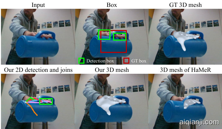
Figure 5. Visualization of HO3Dv3 with actual detection box. We claim that using GT box (red) for downstream tasks is ill-suited.
| Method | PJ← | PV↓ | AUC↑ |
| Spurr et al. [55] | 6.8 | 0.864 | |
| MobRecon [8] HandOccNet[47] | 6.4 | 5.6 | |
| H2ONet [64] | 5.8 | 5.5 | |
| Zhouetal.[79] | 5.7 | 5.5 | |
| 5.5 | 5.5 | ||
| HandOS (ours) | 5.2 | 5.0 | 0.896 |
Table 4. Results on DexYCB. Errors are measured in mm.
图 5: 带有实际检测框的HO3Dv3可视化效果。我们认为在下游任务中使用GT框(红色)并不合适。
| 方法 | PJ← | PV↓ | AUC↑ |
|---|---|---|---|
| Spurr et al. [55] | 6.8 | 0.864 | |
| MobRecon [8] HandOccNet[47] | 6.4 | 5.6 | |
| H2ONet [64] | 5.8 | 5.5 | |
| Zhouetal.[79] | 5.7 | 5.5 | |
| 5.5 | 5.5 | ||
| HandOS (ours) | 5.2 | 5.0 | 0.896 |
表 4: DexYCB上的结果。误差以毫米为单位。
In contrast, we do not rely on the assumption of perfect detection, and our one-stage pipeline can generate reasonable results from an imperfect box, as shown in Fig. 5.
相比之下,我们并不依赖完美检测的假设,且我们的单阶段流程能从有缺陷的边界框生成合理结果,如图 5 所示。
DexYCB. We use DexYCB to further validate the HandOS for object manipulation. As shown in Table 4, we achieve a clear advantage in accuracy over related methods.
DexYCB。我们使用DexYCB进一步验证HandOS在物体操控中的性能。如表4所示,本方法在精度上较现有方法具有明显优势。
Hint. We utilize the HInt benchmark with New Days, VISOR, and Ego4D to evaluate HandOS on daily-life images using 2D PCK. In our method, 2D joints can be directly predicted through 2D queries or derived via 3D mesh projection. Accordingly, we report both types of PCK in Table 5. Compared to prior arts [14, 49], our training dataset is a subset of theirs, with less than one-tenth of their data size. Despite this, HandOS outperforms HaMeR and Hamba across most PCK metrics. Notably, we achieve the highest values on all PCK $\mathbb{Q}0.05$ metrics, underscoring the capability for highly accurate predictions. Additionally, we obtain superior values across all metrics on HInt-Ego4D, highlighting our advantage in handling first-person perspectives.
提示。我们利用HInt基准测试中的New Days、VISOR和Ego4D数据集,通过2D PCK指标评估HandOS在日常生活图像上的表现。在我们的方法中,2D关节点既可通过2D查询直接预测,也可通过3D网格投影间接获得。因此,表5中同时报告了两种PCK结果。相较于现有技术[14,49],我们的训练数据集规模不足其十分之一。尽管如此,HandOS在多数PCK指标上仍优于HaMeR和Hamba。值得注意的是,我们在所有PCK $\mathbb{Q}0.05$ 指标上均取得最高值,这验证了方法的高精度预测能力。此外,在HInt-Ego4D的所有指标上我们都获得更优结果,凸显了处理第一人称视角的优势。
表5:
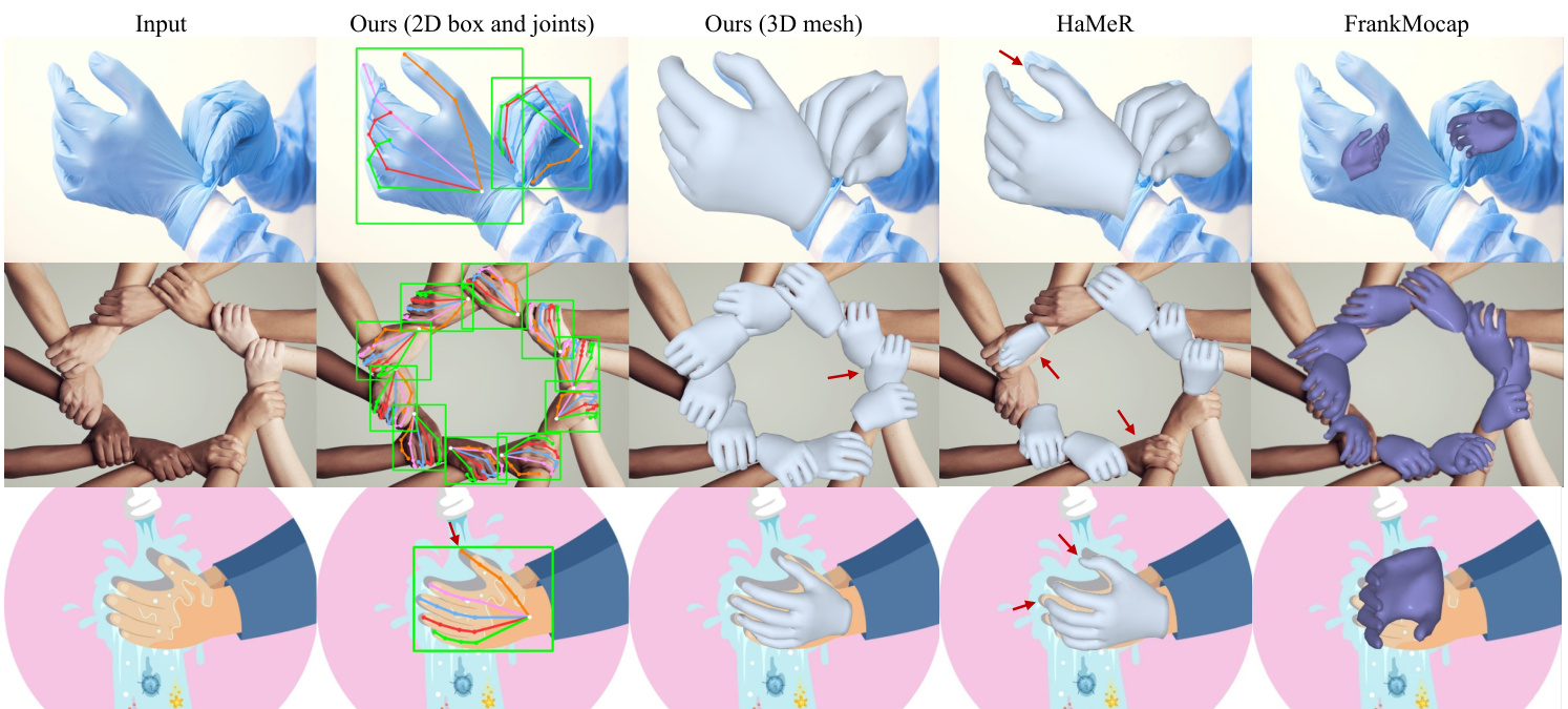
Figure 6. Visual comparison. We are adept at handling long-tail textures, crowded hands, and unseen styles. Red arrows indicate errors.
图 6: 视觉对比。我们擅长处理长尾纹理、密集手部及未见风格。红色箭头标注错误处。
| Method | Data size | Train Hint | NewDays | VISOR | Eg04D | |||||||
| @0.05 | @0.1 | @0.15 | @0.05 | @0.1 | @0.15 | @0.05 | @0.1 | @0.15 | ||||
| Hamba [14] | 2,720K | 48.7 | 79.2 | 90.0 | 47.2 | 80.2 | 91.2 | |||||
| HaMeR [49] | 2,749K | 51.6 | 81.9 | 91.9 | 56.5 | 88.1 | 95.6 | 46.9 | 79.3 | 90.4 | ||
| HandOS-2D (ours) | 204K | 55.8 | 75.8 | 84.5 | 66.2 | 85.3 | 91.8 | 64.6 | 85.3 | 92.8 | ||
| HandOS-proj (ours) | 53.7 | 75.9 | 85.1 | 64.8 | 85.4 | 92.0 | 63.4 | 85.3 | 92.9 | |||
| Visible | Hamba [14] HaMeR [49] | 2,720K | 61.2 | 88.4 | 94.9 | 61.4 | 89.6 | 95.6 | ||||
| HandOS-2D (ours) | 2,749K | 62.9 69.8 | 89.4 85.0 | 95.8 | 66.5 | 92.7 | 97.4 | 59.1 | 87.0 | 94.0 | ||
| HandOS-proj (ours) | 204K | 65.7 | 84.2 | 90.6 90.5 | 80.3 78.1 | 92.5 92.1 | 95.7 95.6 | 79.7 77.4 | 93.1 92.8 | 96.6 96.6 | ||
| Occluc | Hamba [14] HaMeR [49] | 2,720K | 28.2 | 62.8 | 81.1 | 29.9 | 66.6 | 84.3 | ||||
| HandOS-2D (ours) | 2,749K | 33.2 35.5 | 68.4 | 84.8 | 42.6 51.3 | 79.0 | 91.3 | 33.1 46.3 | 69.8 | 84.9 | ||
| HandOS-proj (ours) | 204K | 35.8 | 63.4 64.4 | 76.1 77.5 | 50.6 | 77.9 78.5 | 87.4 88.0 | 46.3 | 75.7 | 86.9 | ||
| 76.1 | 87.3 | |||||||||||
Table 5. Results on HInt. HandOS-2D and HandOS-proj denote the results from our 2D prediction and projected 3D prediction.
| 方法 | 数据量 | 训练提示 | NewDays @0.05 | NewDays @0.1 | NewDays @0.15 | VISOR @0.05 | VISOR @0.1 | VISOR @0.15 | Eg04D @0.05 | Eg04D @0.1 | Eg04D @0.15 | |
|---|---|---|---|---|---|---|---|---|---|---|---|---|
| Hamba [14] | 2,720K | 48.7 | 79.2 | 90.0 | 47.2 | 80.2 | 91.2 | |||||
| HaMeR [49] | 2,749K | 51.6 | 81.9 | 91.9 | 56.5 | 88.1 | 95.6 | 46.9 | 79.3 | 90.4 | ||
| HandOS-2D (ours) | 204K | 55.8 | 75.8 | 84.5 | 66.2 | 85.3 | 91.8 | 64.6 | 85.3 | 92.8 | ||
| HandOS-proj (ours) | 53.7 | 75.9 | 85.1 | 64.8 | 85.4 | 92.0 | 63.4 | 85.3 | 92.9 | |||
| Visible | Hamba [14] HaMeR [49] | 2,720K | 61.2 | 88.4 | 94.9 | 61.4 | 89.6 | 95.6 | ||||
| HandOS-2D (ours) | 2,749K | 62.9 69.8 | 89.4 85.0 | 95.8 | 66.5 | 92.7 | 97.4 | 59.1 | 87.0 | 94.0 | ||
| HandOS-proj (ours) | 204K | 65.7 | 84.2 | 90.6 90.5 | 80.3 78.1 | 92.5 92.1 | 95.7 95.6 | 79.7 77.4 | 93.1 92.8 | 96.6 96.6 | ||
| Occluc | Hamba [14] HaMeR [49] | 2,720K | 28.2 | 62.8 | 81.1 | 29.9 | 66.6 | 84.3 | ||||
| HandOS-2D (ours) | 2,749K | 33.2 35.5 | 68.4 | 84.8 | 42.6 51.3 | 79.0 | 91.3 | 33.1 46.3 | 69.8 | 84.9 | ||
| HandOS-proj (ours) | 204K | 35.8 | 63.4 64.4 | 76.1 77.5 | 50.6 | 77.9 78.5 | 87.4 88.0 | 46.3 | 75.7 | 86.9 | ||
| 76.1 | 87.3 |
表 5. HInt 数据集上的结果。HandOS-2D 和 HandOS-proj 分别表示我们的二维预测和投影三维预测结果。
By comparing HandOS-2D and HandOS-proj in Table 5, it can be concluded that 2D predictions perform better on visible joints, while 3D predictions excel on occluded joints, benefiting from the underlying geometric structure.
通过对比表5中的HandOS-2D和HandOS-proj可以得出:二维预测在可见关节上表现更优,而得益于底层几何结构的三维预测在遮挡关节上更具优势。
Qualitative results. As shown in Fig. 6, compared with HaMeR [49] and FrankMocap [53],the HandOS can handle complex tasks with long-tail texture, crowded objects, and unseen styles. Even without explicitly classifying left and right hands, we still achieve mostly correct results of leftright awareness and mesh reconstruction in a challenging sample, as shown in the 2nd row. Note that cartoon samples are not involved in our training. Hence, the 3rd row shows our ability to zero-shot generalization across styles.
定性结果。如图 6 所示,与 HaMeR [49] 和 FrankMocap [53] 相比,HandOS 能够处理具有长尾纹理、拥挤物体和未见风格的复杂任务。即使没有明确区分左右手,我们仍在一个具有挑战性的样本中实现了基本正确的左右感知和网格重建结果,如第二行所示。需要注意的是,卡通样本并未包含在我们的训练数据中,因此第三行展示了我们在跨风格零样本 (Zero-shot) 泛化方面的能力。
| Qinst Quni | F4 F B SwinT|New Days VISOR Ego4D | ||
| √ | 人人 | 73.8 | 82.5 86.7 |
| 人 | 人人 | 71.9 | 80.7 86.5 |
| √ | 71.5 | 79.5 85.9 | |
| 64.7 | 75.6 80.1 |
Table 6. Ablation studies on side tuning and feature selection. The number is measured at $\mathrm{PCK@0.1}$ . $\boldsymbol{{\mathbf{\ell}}}^{\mathrm{{B}}^{v}}$ ,SwinT” means that $\mathbf{F}^{s}$ is from the pre-trained visual backbone or a from-scratch SwinT.
表 6: 侧调谐和特征选择的消融研究。数值以 $\mathrm{PCK@0.1}$ 为单位测量。$\boldsymbol{{\mathbf{\ell}}}^{\mathrm{{B}}^{v}}$ ,SwinT"表示 $\mathbf{F}^{s}$ 来自预训练的视觉主干或从头训练的SwinT。
Besides, referring to Fig. 5, HandOS can effectively handle imperfect detection results in occluded scenes. Compared with HaMeR, Fig. 5 can also reflect our one-stage superiority in eliminating cumulative errors.
此外,参考图 5,HandOS 能有效处理遮挡场景下的不完美检测结果。与 HaMeR 相比,图 5 也反映出我们在消除累积误差方面的一阶段优势。
4.3. Ablation Studies
4.3. 消融研究
On pre-trained detector. We adapt a pre-trained Grounding DINO for keypoint estimation, making it essential to in- vestigate how the pre-trained model aligns with the downstream task. Key configurations, including query and feature selection as well as side tuning, are examined by a 2D pose model, with their ablation studies detailed in Table 6.
关于预训练检测器。我们采用预训练的 Grounding DINO 进行关键点检测,因此研究预训练模型如何与下游任务对齐至关重要。通过二维姿态模型验证了关键配置(包括查询与特征选择以及侧边调优),其消融实验细节见表 6。

Figure 7. Query lifting matrix. Tips and roots are arranged in the order of thumb, forefinger, middle finger, ring finger, and pinky. The vertex and joint indices follow MANO and MPII orders.
图 7: 查询提升矩阵。指尖和指根按拇指、食指、中指、无名指和小指的顺序排列。顶点和关节索引遵循 MANO 和 MPII 顺序。
We use instance queries $\mathbf{Q}^{i n s t}\in\mathbb{R}^{K\times d^{q}}$ to produce keypoint queries. In another way, keypoint queries can be shared across instances. Hence, we design a unified query $\mathbf{Q}^{u n i}\in\mathbb{R}^{1\times d^{q}}$ , which is applied to $K$ selected instance with respective reference boxes. In addition, different from $\mathbf{Q}^{i n s t}$ that is given by the detector, $\mathbf{Q}^{u n i}$ can be optimized along with the decoder. Referring to the first and second rows of Table 6, $\mathbf{Q}^{i n s t}$ has advantages over $\mathbf{Q}^{u n i}$ . That is, compared to $\mathbf{Q}^{u n i}$ , $\mathbf{Q}^{i n s t}$ has instance-specific information that reduces confusion among instances.
我们使用实例查询 $\mathbf{Q}^{i n s t}\in\mathbb{R}^{K\times d^{q}}$ 来生成关键点查询。另一种方式是让关键点查询在不同实例间共享。因此,我们设计了一个统一查询 $\mathbf{Q}^{u n i}\in\mathbb{R}^{1\times d^{q}}$ ,它会被应用到 $K$ 个选定实例及其对应的参考框上。此外,与检测器提供的 $\mathbf{Q}^{i n s t}$ 不同, $\mathbf{Q}^{u n i}$ 可以随解码器一起优化。参考表 6 的第一行和第二行, $\mathbf{Q}^{i n s t}$ 相比 $\mathbf{Q}^{u n i}$ 更具优势。也就是说,相较于 $\mathbf{Q}^{u n i}$ , $\mathbf{Q}^{i n s t}$ 包含实例特定信息,能减少实例间的混淆。
As shown in the first and third rows of Table 6, ${\bf{F}}{6}^{e}$ outperforms ${\bf F}{4}^{e}$ when used as the value for deformable attention. Since ${\bf{F}}{6}^{e}$ is the deepest representation, it is signifi- cantly influenced by detection training, making it less optimal for keypoint estimation that demands a finer representation of object details. Nevertheless, detailed features can be supplemented through side tuning, enabling ${\bf{F}}_{6}^{e}$ that has the richest semantics to achieve superior performance.
如表 6 第 1 行和第 3 行所示,将 ${\bf{F}}{6}^{e}$ 作为可变形注意力 (deformable attention) 的值时,其性能优于 ${\bf F}{4}^{e}$。由于 ${\bf{F}}{6}^{e}$ 是最深层的表征,受检测训练的显著影响,使其对需要更精细物体细节表征的关键点估计任务表现欠佳。然而,通过侧边调谐 (side tuning) 可以补充细节特征,从而使具有最丰富语义的 ${\bf{F}}_{6}^{e}$ 实现更优性能。
We investigate side tuning by comparing our design with a scratch SwinT network [40]. As shown in the last rows in Table 6, an additional SwinT trained from scratch induces poor performance. This indicates that, despite being trained on the detection task, the shallow features of $\nu$ can be mapped to adapt to other tasks, with detection pretraining also providing positive benefits.
我们通过将设计方案与从头训练的SwinT网络[40]进行对比来研究侧边调谐(side tuning)。如表6最后几行所示,额外从头训练的SwinT网络表现不佳。这表明,尽管是在检测任务上训练的,$\nu$的浅层特征仍可被映射适配其他任务,同时检测预训练也能带来积极收益。
Query lifting. A lifting matrix L is designed to transform 2D joint queries to 3D space. In training, L tends to follow a fixed pattern, and we select several typical lifting patterns for visualization. As illustrated in Fig. 7, the lifting process demonstrates semantic consistency, with the vertex queries originating from those of the corresponding joints.
查询提升。设计了一个提升矩阵L,用于将2D关节查询转换到3D空间。在训练过程中,L倾向于遵循固定模式,我们选取了几种典型的提升模式进行可视化。如图7所示,提升过程展现出语义一致性,顶点查询源自对应关节的查询。

Figure 8. The ablation setting in Table 7. The dark color indicates visible attention computation.
图 8: 表 7 中的消融实验设置。深色部分表示可见的注意力计算。
| Method | New Days | VISOR | Ego4D | FreiHand |
| Fig. 8(a) | 75.1/70.9 | 84.9/81.2 | 84.9/82.1 | 6.4 |
| Fig. 8(b) | 75.7/75.8 | 85.1/85.3 | 85.2/85.2 | 5.7 |
| Fig. 8(c) | 75.8/75.9 | 85.3/85.4 | 85.3/85.3 | 5.6 |
| Fig. 8(d) | 74.6/74.8 | 84.1/84.2 | 84.6/84.5 | 5.9 |
Table 7. Ablation studies on attention strategy. The numbers of the Hint benchmark are $\mathrm{PCK@0.1}$ computed with 2D/projected joints. The numbers of FreiHand is PA-MPVPE in mm.
| 方法 | New Days | VISOR | Ego4D | FreiHand |
|---|---|---|---|---|
| 图 8(a) | 75.1/70.9 | 84.9/81.2 | 84.9/82.1 | 6.4 |
| 图 8(b) | 75.7/75.8 | 85.1/85.3 | 85.2/85.2 | 5.7 |
| 图 8(c) | 75.8/75.9 | 85.3/85.4 | 85.3/85.3 | 5.6 |
| 图 8(d) | 74.6/74.8 | 84.1/84.2 | 84.6/84.5 | 5.9 |
表 7. 注意力策略消融研究。Hint基准的数值为使用2D/投影关节计算的$\mathrm{PCK@0.1}$,FreiHand的数值为PA-MPVPE(单位:毫米)。
Hierarchical attention. Considering the different properties of 2D joints, 3D vertices, and camera translation, we investigate the attention policy and demonstrate the effectiveness of our hierarchical attention, i.e. Fig. 8(c). Compared to it, Fig. 8(a) produces independent attention across different properties; Fig. 8(b) is unidirectional attention; and Fig. 8(d) induces a full attention policy. Referring to Table 7, our design has the best performance in terms of both 2D and 3D metrics. Fig. 8(a) results in a suboptimal 3D learning due to its invisibility to 2D quires. Fig. 8(d) make keypoints relevant to camera position, harming the relative space structure of 2D joints and 3D vertices. Fig. 8(b) has a similar performance to ours, but the interaction among keypoints is insufficient. The necessity of Fig. 8(c) is also exhibited in Table 5, where the 2D prediction is good at visible joints, while the projected estimation is adept at occluded joints. This highlights the importance of information exchange between 2D joints and 3D vertices.
分层注意力机制。考虑到2D关节点、3D顶点和相机平移的不同特性,我们研究了注意力策略并验证了分层注意力的有效性(即图8(c))。相比之下,图8(a)对不同属性采用独立注意力机制;图8(b)为单向注意力;图8(d)则采用全注意力策略。如表7所示,我们的设计在2D和3D指标上均表现最佳。图8(a)由于无法感知2D查询,导致3D学习效果欠佳。图8(d)使关键点与相机位置产生关联,损害了2D关节点与3D顶点的相对空间结构。图8(b)性能与我们的方案相近,但关键点间交互不足。图8(c)的必要性在表5中同样得到体现:2D预测擅长处理可见关节点,而投影估计更适用于遮挡关节点,这凸显了2D关节点与3D顶点间信息交互的重要性。
5. Conclusion
5. 结论
We introduce HandOS, an end-to-end framework for 3D hand mesh reconstruction, which is a unified framework for hand detection, left-right awareness, and pose estimation. Additionally, we propose an interactive 2D-3D de- coder with query expansion, lifting, and hierarchical attention, which supports the concurrent learning of 2D joints, 3D vertices, and camera translation. As a result, HandOS achieves state-of-the-art performance on FreiHand, Ho3Dv3, DexYCB, and HInt benchmarks.
我们介绍了HandOS,这是一个用于3D手部网格重建的端到端框架,它是一个统一的手部检测、左右手识别和姿态估计框架。此外,我们提出了一种带有查询扩展(query expansion)、提升(lifting)和分层注意力(hierarchical attention)的交互式2D-3D解码器,支持2D关节、3D顶点和相机平移的并行学习。因此,HandOS在FreiHand、Ho3Dv3、DexYCB和HInt基准测试中实现了最先进的性能。
Acknowledgment This work was partly supported by the National Natural Science Foundation of China under Grant 62403012, Grant 62233001, Grant U23B2037 and the Postdoctoral Innovative Talent Support Program under Grant BX2023004. The authors acknowledge Ling-Hao Chen for constructive discussions.
致谢
本研究部分得到国家自然科学基金(62403012、62233001、U23B2037)和中国博士后创新人才支持计划(BX2023004)的资助。作者感谢Ling-Hao Chen富有建设性的讨论。
References
参考文献
dataset for markerless capture of hand pose and shape from single RGB images. In ICCV, 2019. 2, 5, 13, 14
用于从单张RGB图像无标记捕捉手部姿态和形状的数据集。发表于ICCV,2019年。2, 5, 13, 14
Abstract
摘要
This is the supplementary document of HandOS, including implementation details (Section VI), metrics (Section VII), discussion on left-right classification (Section VIII), detector adaption (Section IX), and HO3D results (Section X), as well as more comparison (Section XI), efficiency analysis (Section XII), and visual results (Section XIV). Finally, failure cases (Section XIII) and limitations are analyzed (Section XVI).
这是HandOS的补充文档,包含实现细节(第VI节)、指标(第VII节)、左右手分类讨论(第VIII节)、检测器适配(第IX节)和HO3D结果(第X节),以及更多对比(第XI节)、效率分析(第XII节)和可视化结果(第XIV节)。最后分析了失败案例(第XIII节)和局限性(第XVI节)。
VI. Implementation Details
VI. 实现细节
VI.1. Side tuning
VI.1. 侧边调优
As shown in Fig. $\mathrm{IX}$ , we adopt 4-scale feature maps in the visual backbone. For each scale, we utilize 3 convolution layers for feature mapping. Finally, 4-scale mapped features form ${\bf F}_{s}$ .
如图 $\mathrm{IX}$ 所示,我们在视觉主干网络中采用4尺度特征图。每个尺度使用3个卷积层进行特征映射,最终4个尺度的映射特征形成 ${\bf F}_{s}$ 。

Figure IX. The architecture of side tuning.
图 IX: Side tuning 架构图。
VI.2. Loss function and Training
VI.2. 损失函数与训练
The full loss function is given as follows,
完整损失函数如下所示,
$$
\begin{array}{r l}&{\mathcal{L}=\lambda^{{\mathbf{J}^{2D}}}\mathcal{L}^{{\mathbf{J}^{2D}}}+\lambda_{O K S}^{2D}\mathcal{L}_{O K S}^{2D}}\ &{\phantom{{=}}+\lambda^{{\mathbf{V}}}\mathcal{L}^{{\mathbf{V}}}+\lambda^{{\mathbf{J}^{3D}}}\mathcal{L}^{{\mathbf{J}^{3D}}}}\ &{\phantom{{=}}+\lambda^{n o m r a l}\mathcal{L}^{n o m r a l}+\lambda^{e d g e}\mathcal{L}^{e d g e}}\ &{\phantom{{=}}+\lambda^{{\mathbf{J}^{p r o j}}}\mathcal{L}^{{\mathbf{J}^{p r o j}}}+\lambda_{O K S}^{p r o j}\mathcal{L}_{O K S}^{p r o j}}\ &{\phantom{{=}}+\lambda^{n c}\mathcal{L}^{n c},}\end{array}
$$
$$
\begin{array}{r l}&{\mathcal{L}=\lambda^{{\mathbf{J}^{2D}}}\mathcal{L}^{{\mathbf{J}^{2D}}}+\lambda_{O K S}^{2D}\mathcal{L}_{O K S}^{2D}}\ &{\phantom{{=}}+\lambda^{{\mathbf{V}}}\mathcal{L}^{{\mathbf{V}}}+\lambda^{{\mathbf{J}^{3D}}}\mathcal{L}^{{\mathbf{J}^{3D}}}}\ &{\phantom{{=}}+\lambda^{n o m r a l}\mathcal{L}^{n o m r a l}+\lambda^{e d g e}\mathcal{L}^{e d g e}}\ &{\phantom{{=}}+\lambda^{{\mathbf{J}^{p r o j}}}\mathcal{L}^{{\mathbf{J}^{p r o j}}}+\lambda_{O K S}^{p r o j}\mathcal{L}_{O K S}^{p r o j}}\ &{\phantom{{=}}+\lambda^{n c}\mathcal{L}^{n c},}\end{array}
$$
where λJ2D $\lambda^{\mathbf{J}^{2D}}=\lambda^{\mathbf{J}^{3D}}=\lambda^{\mathbf{J}^{\mathbf{V}}}=\lambda^{\mathbf{J}^{\mathbf{V}\scriptscriptstyle2j}}=\lambda^{e d g e}=10.$ , $\lambda_{O K S}^{2D}=\lambda_{O K S}^{p r o j}=4.$ , $\lambda^{n o r m a l}=5$ , $\lambda^{n c}=0.5$ .
其中 λJ2D $\lambda^{\mathbf{J}^{2D}}=\lambda^{\mathbf{J}^{3D}}=\lambda^{\mathbf{J}^{\mathbf{V}}}=\lambda^{\mathbf{J}^{\mathbf{V}\scriptscriptstyle2j}}=\lambda^{e d g e}=10.$ , $\lambda_{O K S}^{2D}=\lambda_{O K S}^{p r o j}=4.$ , $\lambda^{n o r m a l}=5$ , $\lambda^{n c}=0.5$ .
The HandOS can be trained in an end-to-end manner with $\mathcal{L}$ . To accelerate convergence and reduce experimental time, we adopt a two-stage training. First, a 2D model is trained, whose results are reported in Table 6 of the main text. The 2D model also follows the overall architecture in Fig. 2 of the main text, with all interactive layers replaced by 2D layers. Also, the 2D model does not involve query lifting and 3D vertices/camera prediction. The training data include HInt [49], COCO [29], and OneHand10K [62], with the loss function of $\lambda^{{\bf J}^{2D}}\bar{\mathcal{L}^{{\bf J}^{2D}}}+\lambda_{O K S}^{2D}\mathcal{L}_{O K S}^{2D}$ . The 2D training cost 3 days on 8 NVIDIA A100 GPUs.
HandOS 可以通过 $\mathcal{L}$ 进行端到端训练。为加速收敛并减少实验时间,我们采用两阶段训练策略:首先训练一个二维模型(其结果见正文表6),该模型同样遵循正文图2的整体架构,但将所有交互层替换为二维层,且不涉及查询提升与三维顶点/相机预测。训练数据包含 HInt [49]、COCO [29] 和 OneHand10K [62],损失函数为 $\lambda^{{\bf J}^{2D}}\bar{\mathcal{L}^{{\bf J}^{2D}}}+\lambda_{O K S}^{2D}\mathcal{L}_{O K S}^{2D}$。二维训练在8块NVIDIA A100 GPU上耗时3天。
Then, with the weights of the 2D model for initialization, we conduct our experiments on diverse benchmarks with their respective training data.
然后,我们使用2D模型的权重进行初始化,在各自训练数据的不同基准上开展实验。
Ablation studies of loss functions are present in Table VIII. $\mathcal{L}_{O K S}$ improves the 2D learning efficiency from various-size instances. $\mathcal{L}^{s p}=\mathcal{L}^{n o r m a l}+\mathcal{L}^{e d g e}$ is crucial for structural shape learning, while $\mathcal{L}^{n c}$ is a smooth regularization. Other losses are strictly required.
损失函数的消融研究如表 VIII 所示。$\mathcal{L}_{O K S}$ 提升了不同尺寸实例的 2D 学习效率。$\mathcal{L}^{s p}=\mathcal{L}^{n o r m a l}+\mathcal{L}^{e d g e}$ 对结构形状学习至关重要,而 $\mathcal{L}^{n c}$ 是平滑正则项。其他损失函数均为严格必需项。
| LoKS | Cnc | Csp | Eg04D2D-PCK | FreiHandpv |
| √ | √ | 85.3 | 5.6 | |
| √ | 83.2 | 5.8 | ||
| 83.2 | 5.9 | |||
| 82.9 | 13.2 |
| LoKS | Cnc | Csp | Eg04D2D-PCK | FreiHandpv |
|---|---|---|---|---|
| √ | √ | 85.3 | 5.6 | |
| √ | 83.2 | 5.8 | ||
| 83.2 | 5.9 | |||
| 82.9 | 13.2 |
Table VIII. Ablation study of loss functions.
表 VIII: 损失函数的消融研究
VII. Metrics
VII. 指标
Percentage of correctly localized keypoints (PCK) is a metric used to evaluate the accuracy of 2D keypoint localization. A keypoint is considered correct if the distance between its predicted and ground truth locations is below a specified threshold. We use a threshold of 0.05, 0.1, and 0.15 box size, i.e. PCK $@0.05$ , PCK $ @0.1$ , and PCK $@0.15$ .
正确定位关键点的百分比 (PCK) 是用于评估2D关键点定位准确性的指标。当预测关键点与真实关键点之间的距离低于指定阈值时,该关键点被视为正确。我们使用0.05、0.1和0.15倍边界框尺寸作为阈值,即PCK $@0.05$、PCK $@0.1$和PCK $@0.15$。
Mean per joint/vertex position error (MPJPE/MPVPE) measures the mean per joint/vertex error by Euclidean distance (mm) between the estimated and ground-truth coordinates. Since some global variation cannot be induced from a monocular image, we use Procrustes analysis [20] to focus on local precision, i.e., PA-MPJPE/MPVPE.
平均每关节/顶点位置误差 (MPJPE/MPVPE) 通过估计坐标与真实坐标之间的欧氏距离 (mm) 来衡量每个关节/顶点的平均误差。由于单目图像无法推导出某些全局变化,我们使用普氏分析 [20] 来关注局部精度,即 PA-MPJPE/MPVPE。
F-score represents the harmonic mean of recall and precision calculated between two meshes with respect to a specified distance threshold. Specifically, $\mathrm{F}@5$ and $\mathrm{F}@15$ correspond to thresholds of $5\mathrm{mm}$ and $15\mathrm{mm}$ , respectively.
F-score表示两个网格之间在指定距离阈值下的召回率 (recall) 和精确率 (precision) 的调和平均数。具体来说,$\mathrm{F}@5$和$\mathrm{F}@15$分别对应$5\mathrm{mm}$和$15\mathrm{mm}$的阈值。
Area under the curve (AUC) represents the area under the PCK curve plotted against error thresholds ranging from 0 to $50\mathrm{mm}$ with 100 steps.
曲线下面积 (AUC) 表示在误差阈值从0到$50\mathrm{mm}$范围内以100步长绘制的PCK曲线下方的面积。
VIII. Discussion on Left-Right Classification
VIII. 左右分类讨论
The recognition of left and right hands is a difficult task. Previous works usually achieve this with body prior [65]. That is, the left and right are easy to understand with wholebody structure. However, there are many scenarios in which the hand appears without a body, such as in egocentric scenes. Here, the classification error increases, harming the performance of the multi-stage method.
左右手的识别是一项困难的任务。先前的研究通常通过身体先验 [65] 来实现这一点。也就是说,借助全身结构可以轻松区分左右。然而,在许多场景中手部出现时并不伴随身体,例如在第一人称视角场景中。这种情况下分类错误会增加,从而影响多阶段方法的性能。
Our one-stage pipeline is free from the impact of prior left-right information and uses the normal direction to obtain the left-right category based on the reconstructed mesh. In this manner, as long as the reconstruction results are correct, the left-right hand classification is also accurate.
我们的一阶段流程不受先前左右信息的影响,利用法线方向基于重建网格获取左右类别。通过这种方式,只要重建结果正确,左右手分类也能准确完成。
Compared with the previous “left/right $\rightarrow$ mesh” paradigm, our “mesh $\rightarrow$ left/right” investigates another way for hand-side understanding. As a result, our method is superior in left-right classification. Based on the HInt test set, ViTPose [65] achieves a detection recall of $94.6%$ and left-right classification precision of $93.8%$ with its default settings. In contrast, the HandOS based on Grounding DINO reaches a detection recall of $100%$ (with a confidence threshold of 0.1) and left-right classification precision of $97.9%$ . Note that the detection precision cannot be calculated since Hint does not label all positive instances in an image.
与之前的“左/右 $\rightarrow$ 网格”范式相比,我们的“网格 $\rightarrow$ 左/右”探索了另一种手部理解方式。因此,我们的方法在左右分类上表现更优。基于HInt测试集,ViTPose [65] 在其默认设置下实现了 $94.6%$ 的检测召回率和 $93.8%$ 的左右分类准确率。相比之下,基于Grounding DINO的HandOS达到了 $100%$ 的检测召回率(置信度阈值为0.1)和 $97.9%$ 的左右分类准确率。需要注意的是,由于HInt未标注图像中的所有正样本,因此无法计算检测准确率。
IX. Adaptation of Other Detector
IX. 其他检测器的适配
We use DINO-X [? ] as the detector to build the HandOS, which achieve 0.428 box AP when measuring hand category [29] on COCO val2017 [37]. The metrics are shown in Table IX, and it is evident that our HandOS is adaptable to all DETR-like detectors.
我们使用 DINO-X [?] 作为检测器构建 HandOS,在 COCO val2017 [37] 数据集上测量手部类别时达到 0.428 框 AP [29]。相关指标如表 IX 所示,显然我们的 HandOS 能适配所有类 DETR 检测器。
| Method | New Days | VISOR | Ego4D | FreiHand |
| main text | 75.8/75.9 | 85.3/85.4 | 85.3/85.3 | 5.6 |
| w/ DINO-X | 76.3/76.5 | 84.8/84.6 | 85.6/85.5 | 5.5 |
| 方法 | New Days | VISOR | Ego4D | FreiHand |
|---|---|---|---|---|
| 主文本 | 75.8/75.9 | 85.3/85.4 | 85.3/85.3 | 5.6 |
| 使用 DINO-X | 76.3/76.5 | 84.8/84.6 | 85.6/85.5 | 5.5 |
Table IX. The numbers of the Hint benchmark are $\mathrm{PCK@0.1}$ computed with 2D/projected joints. The numbers of FreiHand is PAMPVPE in mm.
表 IX. Hint 基准数据为使用 2D/投影关节计算的 $\mathrm{PCK@0.1}$ 值。FreiHand 数据单位为毫米 (PAMPVPE)。
X. More HO3Dv3 Analysis
X. HO3Dv3 更多分析
As explained in Fig. 5 of the main text, the inference with the ground-truth box is ill-suited, which is prevalent ly employed by previous work. We do not follow this setting and use the actual detection box for inference. In addition, the misaligned detection and ground truth could also induce adverse effects for HandOS training, i.e., query filtering based on ground truth becomes less efficient during training. Despite these unfavorable conditions, the HandOS still reaches superior results, e.g. 8.4 PA-MPJPE.
如正文图5所示,使用真实边界框(ground-truth box)进行推理的方式存在明显缺陷,但该方法在先前工作中被广泛采用。我们未沿用该设定,而是采用实际检测框进行推理。此外,检测框与真实标注的错位也会对HandOS训练产生负面影响,例如基于真实标注的查询过滤机制在训练过程中效率降低。尽管存在这些不利条件,HandOS仍取得了优异成果(如8.4 PA-MPJPE)。
Also, it is necessary to evaluate the model performance with Ho3Dv3 GT boxes. As shown, although GT boxes are not involved in training, the inference can adapt to them, thanks to adaptive within-box feature localization of deformable attention, indicating our robustness to box changes.
此外,还需使用 Ho3Dv3 GT 框评估模型性能。如图所示,尽管训练过程中未涉及 GT 框,但由于可变形注意力 (deformable attention) 的自适应框内特征定位能力,推理过程仍能适配这些框,这表明我们的方法对框变化具有鲁棒性。
To relieve the issue during training, we employ more training data, including FreiHand [81], HInt [49], COCO [29], OneHand10K [62], HO3Dv3 [22], DexYCB [6],
为了缓解训练过程中的问题,我们采用了更多训练数据,包括 FreiHand [81]、HInt [49]、COCO [29]、OneHand10K [62]、HO3Dv3 [22]、DexYCB [6]
CompHand [8], and $\mathrm{H}_{2}\mathrm{O}3\mathrm{D}$ [23]. As shown in Table X, we achieve state-of-the-art numeric results. Note that our combined training data contains 933K samples, which is smaller than that of Hamba with 2,720K samples.
CompHand [8] 和 $\mathrm{H}_{2}\mathrm{O}3\mathrm{D}$ [23]。如表 X 所示,我们取得了最先进的数值结果。需要注意的是,我们的组合训练数据包含 933K 样本,比 Hamba 的 2,720K 样本要少。
| Method | PJ ← PV √ | F@5↑ | F@15↑ |
| AMVUR [28] | 8.7 8.3 | 0.593 | 0.964 |
| Hamba * [14] | 6.9 6.8 | 0.681 | 0.982 |
| HandOS (ours) w/GTbox(ours) | 8.4 8.4 8.4 8.5 | 0.584 0.581 | 0.962 0.962 |
| HandOs*(ours) | 6.8 6.7 | 0.688 | 0.983 |
Table X. Results on HO3Dv3. Errors are measured in mm. * denotes using extra training data.
| 方法 | PJ ← PV √ | F@5↑ | F@15↑ |
|---|---|---|---|
| AMVUR [28] | 8.7 8.3 | 0.593 | 0.964 |
| Hamba * [14] | 6.9 6.8 | 0.681 | 0.982 |
| HandOS (ours) w/GTbox(ours) | 8.4 8.4 8.4 8.5 | 0.584 0.581 | 0.962 0.962 |
| HandOs*(ours) | 6.8 6.7 | 0.688 | 0.983 |
表 X. HO3Dv3数据集上的结果。误差单位为毫米。*表示使用了额外训练数据。
XI. More Qualitative Comparison with HaMeR
XI. 与HaMeR的更多定性比较
More comparisons of HandOS and HaMeR are presented in Fig. X, where we are superior in accurate detection (A), novel-style adaptation (B), fine image alignment with accurate pose/shape (C, D), and reasonable occlusion awareness (E, F).
图 X 展示了 HandOS 与 HaMeR 的更多对比结果,我们在以下方面表现更优:精确检测 (A)、新风格适应 (B)、精准姿态/形状的精细图像对齐 (C, D) 以及合理的遮挡感知 (E, F)。

Figure X. Visual comparison between HandOS and HaMeR
图 X: HandOS 与 HaMeR 的视觉对比
XII. Comparison of Inference Efficiency.
XII. 推理效率对比
With $P,H$ denoting the number of person and hand, our detector+decoder has $(301+108H)\mathrm{{G}}$ FLOPs, using 8G memory; ViTPose+HaMeR has $(484P+244H)\mathrm{G}$ FLOPs, using 12G memory. On RTX3090 and PyTorch, our detector takes 0.5s, and decoder time is from 0.1s $(H{=}1)$ to 0.7s $\scriptstyle{\mathit{M}}=10)$ ); VitPose+HaMeR takes $0.4\substack{+0.06P+0.1H)s}$ .
设 $P,H$ 分别表示人数和手部数量,我们的检测器+解码器具有 $(301+108H)\mathrm{{G}}$ FLOPs,占用8G内存;ViTPose+HaMeR 具有 $(484P+244H)\mathrm{G}$ FLOPs,占用12G内存。在RTX3090和PyTorch环境下,我们的检测器耗时0.5秒,解码时间从0.1秒 $(H{=}1)$ 到0.7秒 $\scriptstyle{\mathit{M}}=10)$;ViTPose+HaMeR 耗时 $0.4\substack{+0.06P+0.1H)s}$。
XIII. Failure Cases
XIII. 失败案例
As shown in Fig. XI, the HandOS could fail in false positive (the 1st row), left-right awareness (the 2nd row), inaccurate pose (the 3rd row), and geometry artifacts (the 4th row), when handling extreme lighting, occlusion, and shape conditions.
如图 XI 所示,HandOS 在处理极端光照、遮挡和形状条件时可能出现误报 (第 1 行)、左右感知错误 (第 2 行)、姿态不准确 (第 3 行) 和几何伪影 (第 4 行) 等问题。

Figure XI. Failure cases. Red arrows indicate errors. Samples in a triplet are input, 2D detection and joints, and 3D mesh.
图 XI: 失败案例。红色箭头标注错误区域。三联样本依次为输入图像、2D检测与关节点、3D网格。
XIV. Qualitative Results
XIV. 定性结果
Referring to Fig. XII–XV, we illustrate samples in our used datasets. As shown, the HandOS can handle various scenarios with hard poses, object occlusion, and etc. We also demonstrate that our HandOS is capable of real-world applications for difficult textures, shapes, lighting, and styles, as shown in Fig. XVI. The model for Fig. XVI is trained with FreiHand [81], HInt [49], CompHand [8], COCO [29], OneHand10K [62]. Note that the HandOS exhibits zeroshot generation across styles (e.g., painting, cartoon), benefiting from the open-world representation of Grounding DINO [39].
参考图 XII-XV,我们展示了所用数据集中的样本。如图所示,HandOS能够处理各种复杂场景,包括困难姿态、物体遮挡等情况。我们还证明了HandOS在实际应用中能够应对困难纹理、形状、光照和风格,如图 XVI 所示。图 XVI 的模型使用 FreiHand [81]、HInt [49]、CompHand [8]、COCO [29] 和 OneHand10K [62] 进行训练。值得注意的是,得益于 Grounding DINO [39] 的开放世界表征能力,HandOS 能够实现跨风格(如绘画、卡通)的零样本生成。
XV. Supplemental Video
XV. 补充视频
Please refer to our homepage for dynamic results, which demonstrates frame-by-frame processing without employing any temporal strategies.
请访问我们的主页查看动态结果,该演示展示了逐帧处理过程,未采用任何时间策略。
XVI. Limitations and Future Works
XVI. 局限性与未来工作
Geometry prior. The HandOS does not incorporate a geometric prior like MANO, meaning that the hand shape is learned entirely from data without relying on any predefined structural knowledge. In our opinion, incorporating an implicit prior (e.g., a variation al auto encoder) could accelerate the convergence of HandOS and improve the geometric realism of the predicted hand geometry.
几何先验。HandOS不像MANO那样包含几何先验,这意味着手的形状完全是从数据中学习而来,不依赖任何预定义的结构知识。我们认为,引入隐式先验(例如变分自编码器)可以加速HandOS的收敛,并提升预测手部几何的逼真度。
Pose representation. We use keypoints to unify left-right hand representation. Nevertheless, obtaining a rotational pose (i.e. $\pmb{\theta}$ in MANO) is less straightforward and requires an extra inverse kinematics module.
姿态表示。我们使用关键点来统一左右手的表示。然而,获取旋转姿态 (即 MANO 中的 $\pmb{\theta}$ ) 不太直接,需要一个额外的逆运动学模块。
Temporal coherence. The HandOS is designed for single image processing without considerations for temporal coherence, which may result in jerky outputs when applied to video inference.
时序一致性。HandOS 专为单张图像处理设计,未考虑时序一致性,因此在应用于视频推理时可能导致输出不流畅。
Future works. We plan to extend HandOS to provide versatile hand understanding. In addition to detection, 2D pose, and 3D mesh, other properties such as segmentation, texture, and object contact are also valuable considerations. Furthermore, the HandOS will be utilized to analyze human manipulation skills, contributing to advancements in embodied intelligence.
未来工作。我们计划扩展HandOS以提供多功能的手部理解能力。除检测、2D姿态和3D网格外,分割、纹理和物体接触等其他属性也是值得考虑的有价值特性。此外,HandOS将被用于分析人类操作技能,推动具身智能 (embodied intelligence) 的发展。

Figure XII. Visualization of FreiHand evaluation set. Samples in a triplet are input, 2D detection and joints, and 3D mesh.
图 XII: FreiHand评估集的可视化。每组三个样本分别为输入图像、2D检测与关节点、3D网格。

Figure XIII. Visualization of HO3Dv3 evaluation set. Samples in a triplet are input, 2D detection and joints, and 3D mesh.
图 XIII: HO3Dv3 评估集可视化。三联样本分别为输入图像、2D检测与关节点、3D网格。

Figure XIV. Visualization of DexYCB test set. Samples in a triplet are input, 2D detection and joints, and 3D mesh.
图 XIV: DexYCB测试集可视化。三联样本分别为输入、2D检测与关节点、3D网格。

Figure XV. Visualization of HInt test set. Samples in a triplet are input, 2D detection and joints, and 3D mesh.
图 XV: HInt测试集可视化。三联样本分别为输入图像、2D检测与关节点、3D网格。

Figure XVI. Visualization of practical application. Samples in a triplet are input, 2D detection and joints, and 3D mesh.
图 XVI: 实际应用可视化。三元组中的样本分别为输入、2D检测与关节点、3D网格。