Recurrent Generic Contour-based Instance Segmentation with Progressive Learning
基于渐进式学习的循环通用轮廓实例分割
Abstract—Contour-based instance segmentation has been actively studied, thanks to its flexibility and elegance in processing visual objects within complex backgrounds. In this work, we propose a novel deep network architecture, i.e., PolySnake, for generic contour-based instance segmentation. Motivated by the classic Snake algorithm, the proposed PolySnake achieves superior and robust segmentation performance with an iterative and progressive contour refinement strategy. Technically, PolySnake introduces a recurrent update operator to estimate the object contour iterative ly. It maintains a single estimate of the contour that is progressively deformed toward the object boundary. At each iteration, PolySnake builds a semantic-rich representation for the current contour and feeds it to the recurrent operator for further contour adjustment. Through the iterative refinements, the contour progressively converges to a stable status that tightly encloses the object instance. Beyond the scope of general instance segmentation, extensive experiments are conducted to validate the effectiveness and general iz ability of our PolySnake in two additional specific task scenarios, including scene text detection and lane detection. The results demonstrate that the proposed PolySnake outperforms the existing advanced methods on several multiple prevalent benchmarks across the three tasks. The codes and pre-trained models are available at https://github.com/fh2019ustc/PolySnake
摘要—基于轮廓的实例分割因其在处理复杂背景中视觉对象时的灵活性与优雅性而受到广泛研究。本文提出了一种新型深度网络架构PolySnake,用于通用型基于轮廓的实例分割。受经典Snake算法启发,该模型通过迭代渐进式轮廓优化策略实现了卓越且稳健的分割性能。技术上,PolySnake采用循环更新算子对目标轮廓进行迭代估计,始终保持单一轮廓预测并通过渐进形变逼近物体边界。每次迭代时,模型会为当前轮廓构建语义丰富的表征,并将其输入循环算子以进一步调整轮廓。经过多次优化迭代,轮廓最终收敛至紧密包围目标实例的稳定状态。除通用实例分割任务外,我们通过大量实验验证了PolySnake在场景文本检测和车道检测两个特定任务中的有效性与泛化能力。实验结果表明,在三大任务的多个主流基准测试中,PolySnake均超越了现有先进方法。代码与预训练模型已开源:https://github.com/fh2019ustc/PolySnake
Index Terms—Contour-based, Progressive Learning, Instance Segmentation, Text Detection, Lane Detection
索引术语—基于轮廓 (Contour-based)、渐进式学习 (Progressive Learning)、实例分割 (Instance Segmentation)、文本检测 (Text Detection)、车道检测 (Lane Detection)
I. INTRODUCTION
I. 引言
Nstance segmentation is a fundamental computer vision task, aiming to recognize each distinct object in an image along with their associated outlines. It is a challenging task due to background clutter, instance ambiguity, and the complexity of object shapes, etc. The advance of instance segmentation benefits a broad range of visual understanding applications, such as autonomous driving [1], [2], [3], augmented reality [4], [5], robotic grasping [6], [7], surface defect detection [8], [9], [10], text recognition [11], [12], [13], and so on. Over the past few years, instance segmentation has been receiving increased attention and significant progress has been made.
实例分割 (instance segmentation) 是一项基础的计算机视觉任务,旨在识别图像中每个独立对象及其对应的轮廓线。由于背景干扰、实例歧义以及物体形状复杂性等因素,该任务具有较高挑战性。实例分割技术的进步为众多视觉理解应用带来了显著提升,例如自动驾驶 [1][2][3]、增强现实 [4][5]、机器人抓取 [6][7]、表面缺陷检测 [8][9][10]、文字识别 [11][12][13] 等。近年来,实例分割领域持续受到广泛关注并取得了重大进展。
In the literature, most of the state-of-the-art methods [14], [15], [16], [17], [18], [19], [20], [21], [22] adopt a two-
在文献中,大多数最先进的方法 [14]、[15]、[16]、[17]、[18]、[19]、[20]、[21]、[22] 采用了两阶段
Hao Feng, Keyi Zhou, Wengang Zhou, Yufei Yin, Qi Sun, and Houqiang Li are with the CAS Key Laboratory of Technology in Geo-spatial Information Processing and Application System, Department of Electronic Engineering and Information Science, University of Science and Technology of China, Hefei, 230027, China. Hao Feng is also with Zhangjiang Laboratory, Shanghai, China. E-mail: {haof, kyzhou2000, yinyufei, sq008} $@$ mail.ustc.edu.cn; ${\mathrm{zhwg,~lihq}}@$ ustc.edu.cn
Hao Feng、Keyi Zhou、Wengang Zhou、Yufei Yin、Qi Sun 和 Houqiang Li 均任职于中国科学技术大学电子工程与信息科学系,中国科学院空天信息处理与应用系统技术重点实验室,合肥,230027。Hao Feng 同时任职于张江实验室,上海。电子邮箱:{haof, kyzhou2000, yinyufei, sq008} $@$ mail.ustc.edu.cn;${\mathrm{zhwg,~lihq}}@$ ustc.edu.cn
Jiajun Deng is with The University of Adelaide, Australian Institute for Machine Learning. E-mail: jiajun.deng@adelaide.edu.au
Jiajun Deng就职于阿德莱德大学澳大利亚机器学习研究所。电子邮箱:jiajun.deng@adelaide.edu.au
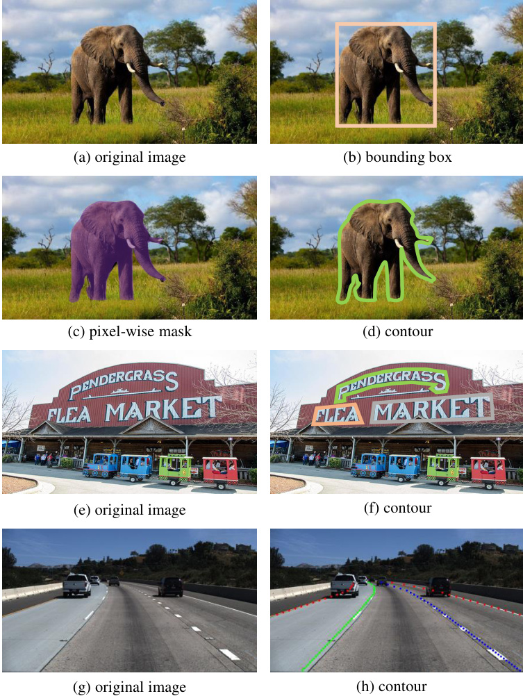
Fig. 1. An illustration of different representations to localize an instance within an image: (b) bounding box; (c) pixel-wise mask; and (d), (f), (h) contour. The images showcase three distinct task scenarios: general instance segmentation (a), scene text detection (f), and lane detection (h).
图 1: 图像中实例定位的不同表示方法示意图:(b) 边界框;(c) 像素级掩码;(d)、(f)、(h) 轮廓。这些图像展示了三种不同的任务场景:通用实例分割 (a)、场景文本检测 (f) 和车道检测 (h)。
stage pipeline for instance segmentation. Typically, they first detect the object instance in the form of bounding boxes (see Fig. 1(b)) and then estimate a pixel-wise segmentation mask (see Fig. 1(c)) within each bounding box. However, the segmentation performance of such methods is limited due to the inaccurate bounding boxes. For example, the classic Mask R-CNN [14] performs a binary classification on a $28\times28$ feature map of a detected instance. Besides, their dense prediction architecture usually suffers from heavy computational overhead [23], limiting their applications in resource-limited scenarios with a real-time requirement.
实例分割的阶段式流水线。通常,它们首先以边界框形式检测对象实例(见图1(b)),然后在每个边界框内估计像素级分割掩码(见图1(c))。然而,由于边界框不准确,这类方法的分割性能受到限制。例如,经典的Mask R-CNN [14] 在检测实例的 $28\times28$ 特征图上执行二元分类。此外,它们的密集预测架构通常面临沉重的计算开销 [23],限制了其在需要实时性的资源受限场景中的应用。
To address the above issues, recent research efforts have been dedicated to designing alternative representations to the pixel-wise segmentation mask. One intuitive representative scheme is the object contour, in the form of a sequence of vertexes along the object silhouette (see Fig. 1(d)). Typically, PolarMask [24], [25] innovative ly applies the angle and distance terms in a polar coordinate system to localize the vertices of the contour, which achieves competitive accuracy. However, in PolarMask [24], [25], contours are constructed from a set of endpoints of concentric rays emitted from the object center, thus restricting the models to handling convex shapes as well as some concave shapes with non-intersecting rays. Another pioneering method is DeepSnake [26] which directly regresses the coordinates of contour vertices in the Cartesian coordinate system. Inspired by the classic Snake algorithm [27], DeepSnake [26] devises a neural network to evolve an initial contour to enclose the object boundary. Nevertheless, the overlarge model size increases the learning difficulty and thus harms the performance. Typically, the performance of DeepSnake [26] drops with more than 4 times contour adjustment. Based on this strong baseline, other methods [28], [29], [30], [31], [32], [33] continue to explore a more effective contour estimation strategy. Although they report promising performance on the challenging benchmarks [34], [35], [36], [37], their contour learning strategies are somewhat heuristic and complex.
为了解决上述问题,最近的研究致力于设计替代逐像素分割掩码的表示方法。一种直观的代表性方案是物体轮廓,即以沿物体轮廓的顶点序列形式呈现(见图1(d))。典型地,PolarMask [24][25]创新性地利用极坐标系中的角度和距离项来定位轮廓顶点,取得了具有竞争力的精度。然而,在PolarMask [24][25]中,轮廓由从物体中心发射的同心射线端点集合构成,因此限制了模型只能处理凸形以及部分射线不相交的凹形。另一项开创性方法是DeepSnake [26],它直接在笛卡尔坐标系中回归轮廓顶点的坐标。受经典Snake算法 [27] 启发,DeepSnake [26] 设计了一个神经网络来演化初始轮廓以包围物体边界。尽管如此,过大的模型尺寸增加了学习难度,从而损害了性能。通常,DeepSnake [26] 的性能在超过4次轮廓调整后会下降。基于这一强基线,其他方法 [28][29][30][31][32][33] 继续探索更有效的轮廓估计策略。尽管它们在具有挑战性的基准测试 [34][35][36][37] 中报告了有希望的性能,但其轮廓学习策略在某种程度上是启发式和复杂的。
In this work, we propose PolySnake, a new deep network architecture for generic contour-based instance segmentation. The idea of our PolySnake is traced back to the classic Snake algorithm [27] that iterative ly deforms an initial polygon to progressively align the object boundary by the optimization of an energy function. Correspondingly, our PolySnake also aims to realize effective automatic contour learning based on iterative and progressive mechanisms simultaneously, different from existing methods. Specifically, given an initial contour of an object instance, PolySnake develops a recurrent update operator to estimate the contour iterative ly. It maintains a single estimate of the contour that is progressively deformed at each iteration. At each iteration, PolySnake first constructs the representation of the contour estimated at the previous iteration. Then, the recurrent operator takes the features as input and estimates the residual displacement to adjust current coarse contour to further outline the object instance. Through the iterative refinements, the contour progressively converges to a stable status that tightly encloses the object instance.
在本工作中,我们提出了PolySnake,这是一种基于通用轮廓的实例分割新深度网络架构。我们PolySnake的灵感可追溯至经典的Snake算法[27],该算法通过能量函数优化迭代地变形初始多边形以逐步贴合目标边界。相应地,我们的PolySnake也旨在基于迭代与渐进机制实现高效的自动轮廓学习,这与现有方法不同。具体而言,给定目标实例的初始轮廓,PolySnake开发了循环更新算子来迭代估计轮廓。它维护着单一轮廓估计,该轮廓在每次迭代中逐步变形。每次迭代时,PolySnake首先构建前一迭代估计的轮廓表征,随后循环算子以这些特征为输入,估计残差位移来调整当前粗糙轮廓以进一步勾勒目标实例。通过迭代优化,轮廓逐步收敛至紧密包围目标实例的稳定状态。
Our PolySnake exhibits a novel design in three aspects, discussed next. Firstly, PolySnake takes a neat network architecture. Due to its recurrent design, the whole model is still lightweight and free from iteration times. Such a lightweight architecture also ensures its real-time ability even under a relatively large number of iterations. Secondly, to achieve a high-quality estimation, we present a multi-scale contour refinement module to further refine the obtained contour by aggregating fine-grained and semantic-rich feature maps. Thirdly, we propose a shape loss to encourage and regularize the learning of object shape, which makes the regressed contour outline the object instance more tightly.
我们的PolySnake在以下三个方面展现出新颖设计。首先,PolySnake采用简洁的网络架构。得益于其循环设计,整个模型仍保持轻量级且不受迭代次数限制。这种轻量架构还确保了即使在较多迭代次数下仍具备实时能力。其次,为实现高质量估计,我们提出多尺度轮廓优化模块,通过聚合细粒度且富含语义的特征图来进一步优化所得轮廓。第三,我们提出形状损失函数以促进和规范物体形状的学习,使回归的轮廓更紧密贴合物体实例。
To evaluate the effectiveness of our PolySnake, we conduct comprehensive experiments on several prevalent instance segmentation benchmark datasets, including SBD [34], Cityscapes [35], COCO [36], and KINS [37]. Furthermore, we validate our PolySnake in other two task scenarios, i.e., scene text detection (see Fig. 1(e, f)) and lane detection (see Fig. 1(g, h)). Distinct from general instance segmentation, scene text detection [38] concentrates solely on segmenting a specific object type, that is text. In lane detection tasks [39], the targeted lane lines inherently lack the closed-loop structure often observed in typical instance segmentation objects. Extensive quantitative and qualitative results demonstrate the merits of our method as well as its superiority over state-ofthe-art methods. Moreover, we validate various design choices of PolySnake through comprehensive studies.
为了评估PolySnake的有效性,我们在多个主流实例分割基准数据集上进行了全面实验,包括SBD [34]、Cityscapes [35]、COCO [36]和KINS [37]。此外,我们还在另外两个任务场景中验证了PolySnake的性能,即场景文本检测(见图1(e, f))和车道线检测(见图1(g, h))。与通用实例分割不同,场景文本检测[38]仅专注于分割特定对象类型——文本。在车道线检测任务[39]中,目标车道线本身缺乏典型实例分割对象常见的闭环结构。大量定量和定性结果证明了我们方法的优势及其相对于最先进方法的优越性。此外,我们通过全面研究验证了PolySnake的各种设计选择。
II. RELATED WORK
II. 相关工作
We mainly discuss the research on instance segmentation in two directions, including mask-based and contour-based. We discuss them in the following.
我们主要从两个方向探讨实例分割的研究,包括基于掩码 (mask-based) 和基于轮廓 (contour-based) 的方法。下文将详细讨论这些内容。
A. Mask-based Instance Segmentation
A. 基于掩码的实例分割
Most recent works perform instance segmentation by predicting pixel-level masks. Some works follow the paradigm of “Detect then Segment” [14], [17], [15], [16], [18], [19], [20], [21], [40]. They usually first detect the bounding boxes and then predict foreground masks in the region of each bounding box. Among them, the classic Mask R-CNN [14] supplements a segmentation branch on Faster R-CNN [41] for per-pixel binary classification in each region proposal. To enhance the feature representation, PANet [17] proposes bottom-up path augmentation to enhance information propagation based on Mask R-CNN [14], and $\mathrm{A^{2}}$ -FPN [20] strengthens pyramidal feature representations through attention-guided feature aggregation. To improve the segmentation parts, Mask Scoring RCNN [16] adds a MaskIoU head to learn the completeness of the predicted masks. HTC [15] and RefineMask [19] integrate cascade into instance segmentation by interweaving detection and segmentation features [15] or fusing the instance features obtained from different stages [19]. Recently, DCT-Mask [18] introduces DCT mask representation to reduce the complexity of mask representation, and BPR [21] proposes the crop-thenrefine strategy to improve the boundary quality.
大多数最新研究通过预测像素级掩码来进行实例分割。部分工作遵循"先检测后分割"范式 [14], [17], [15], [16], [18], [19], [20], [21], [40],通常先检测边界框,然后在每个边界框区域内预测前景掩码。其中经典方法Mask R-CNN [14]在Faster R-CNN [41]基础上增加分割分支,对每个候选区域进行逐像素二分类。为增强特征表示,PANet [17]基于Mask R-CNN提出自底向上路径增强机制来改进信息传播,$\mathrm{A^{2}}$-FPN [20]则通过注意力引导的特征聚合来强化金字塔特征表示。在分割优化方面,Mask Scoring RCNN [16]引入MaskIoU头来学习预测掩码的完整性;HTC [15]和RefineMask [19]分别通过交织检测与分割特征 [15] 或融合多阶段实例特征 [19] 实现级联式实例分割。近期,DCT-Mask [18]采用DCT掩码表示降低复杂度,BPR [21]提出"裁剪-优化"策略来提升边界质量。
There also exist some works that are free of bounding boxes. YOLACT [42] generates several prototype masks over the entire image and predicts a set of coefficients for each instance to combine them. BlendMask [43] directly predicts 2D attention map for each proposal on the top of the FCOS detector [44], and combines them with ROI features. Besides, recent attempts [45], [46], [47], [48] have also applied dynamic convolution kernels trained online, which are then performed on feature maps to generate instance masks.
也存在一些无需边界框的工作。YOLACT [42] 在整个图像上生成多个原型掩码,并为每个实例预测一组系数来组合它们。BlendMask [43] 直接在 FCOS 检测器 [44] 的基础上为每个候选区域预测 2D 注意力图,并将其与 ROI 特征结合。此外,最近的尝试 [45]、[46]、[47]、[48] 还应用了在线训练的动态卷积核,随后在特征图上执行以生成实例掩码。
B. Contour-based Instance Segmentation
B. 基于轮廓的实例分割
Contour-based methods aim to predict a sequence of vertices of object boundaries, which are usually more lightweight than pixel-based methods. Some methods [29], [25], [24] use polar-representation to predict contours directly. Among them, PolarMask [24], [25] extends classic detection algorithm FCOS [44] to instance segmentation, which adds an additional regression head to predict distances from the center point to each boundary vertex. However, performances of such methods are usually limited when dealing with objects with some complex concave shapes. ESE-Seg [29] utilizes Chebyshev polynomials [49] to approximate the shape vector and adds an extra branch on YOLOv3 [50] to regress the coefficients of Chebyshev polynomials.
基于轮廓的方法旨在预测物体边界的一系列顶点,通常比基于像素的方法更轻量。一些方法[29]、[25]、[24]直接采用极坐标表示预测轮廓。其中,PolarMask[24]、[25]将经典检测算法FCOS[44]扩展到实例分割任务,通过增加回归头预测中心点到各边界顶点的距离。但此类方法在处理复杂凹形物体时性能往往受限。ESE-Seg[29]利用切比雪夫多项式[49]逼近形状向量,并在YOLOv3[50]上新增分支回归切比雪夫多项式系数。
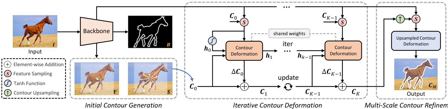
Fig. 2. An overview of the proposed PolySnake framework. PolySnake consists of three modules: Initial Contour Generation (ICG), Iterative Contour Deformation (ICD), and Multi-scale Contour Refinement (MCR). Given an input image $\pmb{I}$ , ICG first initializes a coarse contour $C_{0}$ based on the predicted center heatmap $\mathbf{Y}$ and offset map ${s}$ . Then, in ICD, the obtained contour $C_{0}$ is progressively deformed with $K$ iterations. After that, in MCR, we construct a large-scale but semantic-rich feature map for a further refinement and obtain the output contour $C_{M}$ .
图 2: 提出的PolySnake框架概览。PolySnake包含三个模块: 初始轮廓生成(ICG)、迭代轮廓形变(ICD)和多尺度轮廓优化(MCR)。给定输入图像$\pmb{I}$,ICG首先基于预测的中心热力图$\mathbf{Y}$和偏移图${s}$初始化粗轮廓$C_{0}$。随后在ICD模块中,通过$K$次迭代逐步形变获得的轮廓$C_{0}$。最后在MCR模块中,我们构建大尺度但语义丰富的特征图进行进一步优化,得到输出轮廓$C_{M}$。
Some other works [26], [30], [32], [51], [33] apply Cartesian coordinate representation for vertices, and regress them towards ground-truth object boundaries. Typically, DeepSnake [26] first initializes the contours based on the box predictions, and then applies several contour deformation steps for segmentation. Based on DeepSnake[26], Dance [32] improves the matching scheme between predicted and target contours and introduces an attentive deformation mechanism. ContourRender [51] uses DCT coordinate signature and applies a differentiable renderer to render the contour mesh. Eigencontours [52] proposes a contour descriptor based on low-rank approximation and then incorporates the ei gen contours into an instance segmentation framework. Recently, E2EC [33] applies a novel learnable contour initialization architecture and shows remarkable performance.
其他一些工作[26]、[30]、[32]、[51]、[33]采用笛卡尔坐标系表示顶点,并将其回归到真实物体边界。典型地,DeepSnake[26]首先基于框预测初始化轮廓,然后应用多个轮廓变形步骤进行分割。基于DeepSnake[26],Dance[32]改进了预测轮廓与目标轮廓的匹配方案,并引入了注意力变形机制。ContourRender[51]使用DCT坐标签名,并应用可微分渲染器来渲染轮廓网格。Eigencontours[52]提出了一种基于低秩近似的轮廓描述符,然后将特征轮廓整合到实例分割框架中。最近,E2EC[33]应用了一种新颖的可学习轮廓初始化架构,并展现出卓越性能。
Distinct from existing methodologies, our PolySnake model introduces an innovative iterative and progressive mechanism for learning object contours, thereby achieving precise and robust estimations across a variety of objects.
与现有方法不同,我们的PolySnake模型引入了一种创新的迭代渐进式学习机制来获取物体轮廓,从而实现对各类物体的精准鲁棒估计。
III. METHODOLOGY
III. 方法论
An overview of the proposed PolySnake is shown in Fig. 2. Echoing the methodology of the classic Snake algorithm, PolySnake employs an iterative approach to contour deformation, aiming to precisely align with the object boundary. We develop a recurrent architecture that allows a single estimate of the contour progressively updated at each iteration, and further refine the obtained contour at a larger image scale. Through iterative refinements, the contour steadily envelops the object, eventually stabilizing at a consistent state. For the convenience of understanding, we divide the framework into three modules, including (1) initial contour generation, (2) iterative contour deformation, and (3) multi-scale contour refinement. Each module is discussed in detail in the subsequent sections.
图 2 展示了所提出的 PolySnake 方法概览。延续经典 Snake 算法的思路,PolySnake 采用迭代式轮廓变形策略,旨在实现与物体边界的精确贴合。我们设计了一种循环架构,使得单次轮廓估计能在每次迭代中持续更新,并在更大图像尺度上进一步优化所得轮廓。通过迭代优化,轮廓将逐步包裹目标物体,最终收敛至稳定状态。为便于理解,我们将框架划分为三个模块:(1) 初始轮廓生成,(2) 迭代轮廓变形,(3) 多尺度轮廓优化。后续章节将详细讨论各模块实现。
A. Initial Contour Generation
A. 初始轮廓生成
The Initial Contour Generation (ICG) module is designed to construct preliminary contours for object instances. Leveraging the principles of CenterNet [53], both DeepSnake [26] and Dance [32] initialize a contour from the detected bounding box with a rectangle, whereas E2EC [33] adopts a direct regression of an ordered vertex set to form the initial contour. In our PolySnake, we initialize the coarse contours based on the basic setting of E2EC [33], described next.
初始轮廓生成(ICG)模块旨在为物体实例构建初步轮廓。基于CenterNet[53]的原理,DeepSnake[26]和Dance[32]从检测到的边界框初始化矩形轮廓,而E2EC[33]采用直接回归有序顶点集来形成初始轮廓。在我们的PolySnake中,我们基于E2EC[33]的基本设置初始化粗轮廓,具体描述如下。
Specifically, given an input RGB image $\pmb{I} \in~\mathbb{R}^{H\times W\times3}$ with width $W$ and height $H$ , we first inject it to a backbone network [54], and obtain a feature map $\dot{\pmb{F}}\in\mathbb{R}^{\frac{H}{R}\times\frac{W}{R}\times D}$ , where $R=4$ is the output stride and $D$ denotes the channel number. Then, as shown in Fig. 2, the initial contour is generated with three parallel branches. The first branch predicts a center heatmap $\begin{array}{r}{\dot{\textbf{\emph{Y}}}\in{\bf\Gamma}[0,1]^{\frac{H}{R}\times\frac{W}{R}\times C}}\end{array}$ , where $C$ is the number of object categories. The second branch regresses an offset map $\begin{array}{r l}{S}&{{}\in}&{\mathbb{R}^{\frac{H}{R}\times\frac{W}{R}\times2N_{v}}}\end{array}$ , where $N_{v}$ denotes the vertex number to form an object contour. Let $(x_{i},y_{j})$ denote the center coordinate of an object, then its contour can be obtained by adding the predicted offset ${(\Delta x^{k},\Delta y^{k})|k=1,2,...,N_{v}}$ at $(x_{i},y_{j})$ of $\boldsymbol{S}$ . Moreover, we supplement an extra branch. It predicts a category-agnostic boundary map $\begin{array}{r}{B\in\mathbb{R}^{\frac{H}{R}\times\frac{W}{R}}}\end{array}$ , in which each value is a classification confidence (boundary/nonboundary). Our motivation is that such a branch can help to extract the more fine-grained features for the perception of object boundaries. Note that this branch is only used in the training, which will not cause an extra computation burden for inference. During inference, the instance center can be obtained efficiently based on the max pooling operation [53] on the heatmap $\mathbf{Y}$ . Finally, we obtain the initial contour $C_{0}\in\mathbb{R}^{N_{v}\times2}$ used for the following refinements.
具体来说,给定一个宽度为$W$、高度为$H$的输入RGB图像$\pmb{I} \in~\mathbb{R}^{H\times W\times3}$,我们首先将其输入到主干网络[54]中,获得特征图$\dot{\pmb{F}}\in\mathbb{R}^{\frac{H}{R}\times\frac{W}{R}\times D}$,其中$R=4$为输出步长,$D$表示通道数。接着,如图2所示,初始轮廓通过三个并行分支生成。第一个分支预测中心热图$\begin{array}{r}{\dot{\textbf{\emph{Y}}}\in{\bf\Gamma}[0,1]^{\frac{H}{R}\times\frac{W}{R}\times C}}\end{array}$,其中$C$是目标类别数。第二个分支回归偏移图$\begin{array}{r l}{S}&{{}\in}&{\mathbb{R}^{\frac{H}{R}\times\frac{W}{R}\times2N_{v}}}\end{array}$,其中$N_{v}$表示构成目标轮廓的顶点数。设$(x_{i},y_{j})$为目标中心坐标,则其轮廓可通过在$\boldsymbol{S}$的$(x_{i},y_{j})$处添加预测偏移${(\Delta x^{k},\Delta y^{k})|k=1,2,...,N_{v}}$获得。此外,我们补充了一个额外分支,预测类别无关的边界图$\begin{array}{r}{B\in\mathbb{R}^{\frac{H}{R}\times\frac{W}{R}}}\end{array}$,其中每个值为分类置信度(边界/非边界)。我们的动机是该分支有助于提取更细粒度的特征以感知目标边界。注意此分支仅用于训练,不会增加推理时的计算负担。推理时,实例中心可通过在热图$\mathbf{Y}$上执行最大池化操作[53]高效获得。最终,我们得到用于后续优化的初始轮廓$C_{0}\in\mathbb{R}^{N_{v}\times2}$。
B. Iterative Contour Deformation
B. 迭代轮廓变形
Given the initial contour of an object instance, the Iterative Contour Deformation (ICD) module maintains a single estimation of object contour, which is refined iterative ly. In this way, the initial contour finally converges to a stable state tightly enclosing the object. The architecture of the ICD module is neat, which contributes to the low latency of our method even with a relatively large number of iterations.
给定物体实例的初始轮廓,迭代轮廓变形(ICD)模块会持续维护单一物体轮廓估计,并通过迭代逐步优化。这种方式使得初始轮廓最终收敛至紧密包裹物体的稳定状态。ICD模块架构简洁,即使进行较多轮次迭代,仍能保持方法的低延迟特性。
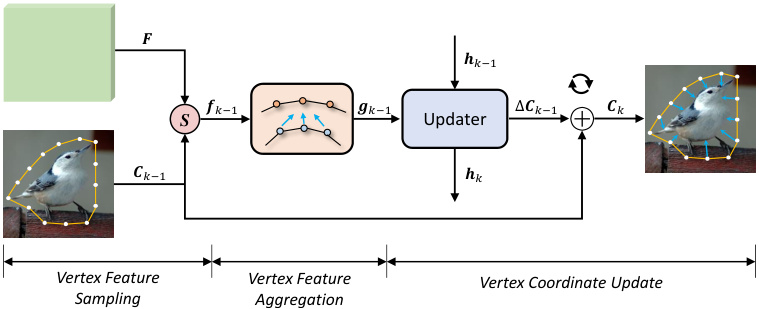
Fig. 3. An illustration of the $k^{t h}$ iteration in the ICD module. “ $\boldsymbol{S}$ ” denotes vertex feature sampling based on bilinear interpolation. “ $\yen123,456$ represents element-wise addition for deforming the current contour.
图 3: ICD模块中第$k^{th}$次迭代的示意图。"$\boldsymbol{S}$"表示基于双线性插值的顶点特征采样。"$\yen123,456$"表示用于变形当前轮廓的逐元素加法。
The workflow of ICD module is illustrated in Fig. 2. Given the feature map $\pmb{F}\in\mathbb{R}^{\frac{H}{R}\times\frac{W}{R}\times D}$ extracted by the backbone network and the initial contour ${\cal C}{0}={p_{0}^{1},\stackrel{.}{p_{0}^{2}},...,p_{0}^{N_{v}}}\in$ $\mathbb{R}^{N_{v}\times2}$ of an object, we deform the object contour iterative ly ${p_{k}^{1},p_{k}^{2},...,p_{k}^{N_{v}}}$ s eiqsu tehnec ep ${C_{1},C_{2},...,C_{K}}$ o, ntwohuerr ew $\begin{array}{r l}{C_{k}}&{{}=}\end{array}$ $N_{v}$ vertices at the $k^{t h}$ iteration, and $K$ is the total iteration number. Note that the two channels of the contour $C_{k}\in\mathbb{R}^{N_{v}\times2}$ denote the horizontal and the vertical coordinates of $N_{v}$ vertices, respectively. After $K$ iterations, we produce the high-quality object contour $C_{K}$ .
ICD模块的工作流程如图2所示。给定骨干网络提取的特征图$\pmb{F}\in\mathbb{R}^{\frac{H}{R}\times\frac{W}{R}\times D}$和物体的初始轮廓${\cal C}{0}={p_{0}^{1},\stackrel{.}{p_{0}^{2}},...,p_{0}^{N_{v}}}\in$ $\mathbb{R}^{N_{v}\times2}$,我们通过迭代变形物体轮廓${p_{k}^{1},p_{k}^{2},...,p_{k}^{N_{v}}}$生成序列${C_{1},C_{2},...,C_{K}}$,其中$C_{k}$表示第$k^{th}$次迭代时的$N_{v}$个顶点,$K$为总迭代次数。需注意轮廓$C_{k}\in\mathbb{R}^{N_{v}\times2}$的两个通道分别表示$N_{v}$个顶点的水平坐标和垂直坐标。经过$K$次迭代后,最终生成高质量物体轮廓$C_{K}$。
As shown in Fig. 3, we illustrate the contour update process at the $k^{t h}$ iteration. Given the feature map $\pmb{F}\in\mathbb{R}^{\frac{\cdot\pmb{H}}{R}\times\frac{W}{R}\times D}$ and the contour $C_{k-1}$ predicted at the ${(k-1)}^{t h}$ iteration, we first sample the vertex-wise feature and then aggregate them for deforming the current contour. We divide the contour update process in ICD module into three sub-processes, including (1) vertex-wise feature sampling, (2) vertex feature aggregation, and (3) vertex coordinate update, as described in the following.
如图 3 所示,我们展示了第 $k^{t h}$ 次迭代时的轮廓更新过程。给定特征图 $\pmb{F}\in\mathbb{R}^{\frac{\cdot\pmb{H}}{R}\times\frac{W}{R}\times D}$ 和第 ${(k-1)}^{t h}$ 次迭代预测的轮廓 $C_{k-1}$,我们首先对顶点特征进行采样,然后聚合这些特征以变形当前轮廓。我们将 ICD 模块中的轮廓更新过程分为三个子过程:(1) 顶点特征采样,(2) 顶点特征聚合,(3) 顶点坐标更新,具体描述如下。
Vertex-wise feature sampling. Given the feature map $\pmb{F}\in\mathbb{R}^{\frac{H}{R}\times\frac{W}{R}\times D}$ of image $\pmb{I}$ and the contour $C_{k-1}\in\mathbb{R}^{N_{v}\times2}$ with $N_{v}$ vertices ${p_{k-1}^{1},p_{k-1}^{2},...,p_{k-1}^{N_{v}}}$ predicted at the (k 1)th iteration, we first retrieve features of these $N_{v}$ vertices. Specifically, given a vertex $\pmb{p}{k-1}^{i}\in\mathbb{R}^{2}$ , we sample its feature vector $F(\pmb{p}{k-1}^{i})\in\mathbb{R}^{D}$ on the feature map $\pmb{F}$ based on the bilinear interpolation. Note that according to classic STN [55], we can compute the gradients to the input $\pmb{F}$ and $C_{k-1}$ for back propagation, thus the module can be trained in an end-to-end manner. After that, we concatenate the feature vectors of the total $N_{v}$ vertices and produce the vertex feature $f_{k-1}\in\mathbb{R}^{N_{v}\times D}$ at the ${(k-1)}^{t h}$ iteration.
逐顶点特征采样。给定图像 $\pmb{I}$ 的特征图 $\pmb{F}\in\mathbb{R}^{\frac{H}{R}\times\frac{W}{R}\times D}$ 和第 $(k-1)$ 次迭代预测的轮廓 $C_{k-1}\in\mathbb{R}^{N_{v}\times2}$ (包含 $N_{v}$ 个顶点 ${p_{k-1}^{1},p_{k-1}^{2},...,p_{k-1}^{N_{v}}}$),我们首先检索这 $N_{v}$ 个顶点的特征。具体而言,给定顶点 $\pmb{p}{k-1}^{i}\in\mathbb{R}^{2}$,我们基于双线性插值从特征图 $\pmb{F}$ 中采样其特征向量 $F(\pmb{p}{k-1}^{i})\in\mathbb{R}^{D}$。根据经典STN [55],可计算输入 $\pmb{F}$ 和 $C_{k-1}$ 的梯度用于反向传播,因此该模块能以端到端方式训练。最后,我们将所有 $N_{v}$ 个顶点的特征向量拼接,生成第 ${(k-1)}^{t h}$ 次迭代的顶点特征 $f_{k-1}\in\mathbb{R}^{N_{v}\times D}$。
Vertex feature aggregation. This module constructs the contour-level representation for $C_{k-1}$ by fusing the vertex features $f_{k-1}$ . Following [26], [32], [33], [38], we use the circle-convolution to fuse the feature of the contour. The circleconvolution operation firstly joins up the head and tail of the input sequence and then applies a standard 1-D convolution on it, which is applicable to capture features of a contour with a polygon topology. In our implementation, we first stack eight circle-convolution layers with residual skip connections for all the layers. Then, we concatenate the features from all the layers and forward them through three $1\times1$ convolutional layers. Finally, we explicitly concatenate the output features with contour coordinate $C_{k-1}\in\mathbb{R}^{N_{v}\times2}$ , obtaining the contour representation $\pmb{g}{k-1}\in\mathbb{R}^{N_{v}\times D_{v}}$ .
顶点特征聚合。该模块通过融合顶点特征$f_{k-1}$为$C_{k-1}$构建轮廓级表示。根据[26]、[32]、[33]、[38],我们采用圆形卷积(circle-convolution)来融合轮廓特征。该操作首先将输入序列首尾相连,然后对其应用标准一维卷积,适用于捕获具有多边形拓扑结构的轮廓特征。具体实现中,我们首先堆叠八个带残差跳跃连接的圆形卷积层,随后拼接所有层的特征并通过三个$1\times1$卷积层。最终将输出特征与轮廓坐标$C_{k-1}\in\mathbb{R}^{N_{v}\times2}$显式拼接,得到轮廓表示$\pmb{g}{k-1}\in\mathbb{R}^{N_{v}\times D_{v}}$。

Fig. 4. Inner structure of the GRU-based vertex coordinate updater.
图 4: 基于GRU的顶点坐标更新器内部结构
Vertex coordinate update. To make the contour enclose the object tightly, we introduce a recurrent update operator that iterative ly updates the currently estimated contour. Fig. 4 illustrates the structure of our GRU-based update operator. It is a gated activation unit based on the GRU cell [56], in which the fully connected layers are replaced with the 1-D convolutional layers. At the $k^{t h}$ iteration, it takes the contour representation $\dot{\pmb{g}}{k-1}\in\mathbb{R}^{N_{v}\times D_{v}}$ as well as the hidden state $\pmb{h}{k-1}\in\mathbb{R}^{N_{v}\times D_{v}}$ as input, differentiates them, and outputs the hidden states $\pmb{h}{k}\in\mathbb{R}^{N_{v}\times D_{v}}$ as follows,
顶点坐标更新。为了使轮廓紧密包围目标物体,我们引入了一种循环更新算子,用于迭代更新当前估计的轮廓。图4展示了基于GRU的更新算子结构。这是一个基于GRU单元[56]的门控激活单元,其中全连接层被一维卷积层取代。在第$k^{t h}$次迭代时,它以轮廓表示$\dot{\pmb{g}}{k-1}\in\mathbb{R}^{N_{v}\times D_{v}}$和隐藏状态$\pmb{h}{k-1}\in\mathbb{R}^{N_{v}\times D_{v}}$作为输入,对它们进行差分处理,并输出隐藏状态$\pmb{h}{k}\in\mathbb{R}^{N_{v}\times D_{v}}$,具体如下:
$$
\begin{array}{r l r}{\lefteqn{z_{k}=\sigma\big(C o n v\big([h_{k-1},g_{k-1}],W_{z}\big)\big),}}\ &{r_{k}=\sigma\big(C o n v\big([h_{k-1},g_{k-1}],W_{r}\big)\big),}\ &{\widetilde{h}{k}=t a n h\big(C o n v\big([r_{k}\odot h_{k-1},g_{k-1}],W_{h}\big)\big),}&\ &{\quad h_{k}=\big(1-z_{k}\big)\odot h_{k-1}+z_{k}\odot\widetilde{h}_{k},}\end{array}
$$
$$
\begin{array}{r l r}{\lefteqn{z_{k}=\sigma\big(C o n v\big([h_{k-1},g_{k-1}],W_{z}\big)\big),}}\ &{r_{k}=\sigma\big(C o n v\big([h_{k-1},g_{k-1}],W_{r}\big)\big),}\ &{\widetilde{h}{k}=t a n h\big(C o n v\big([r_{k}\odot h_{k-1},g_{k-1}],W_{h}\big)\big),}&\ &{\quad h_{k}=\big(1-z_{k}\big)\odot h_{k-1}+z_{k}\odot\widetilde{h}_{k},}\end{array}
$$
where $\odot$ denotes element-wise multiplication; $W_{z}$ , $W_{r}$ , and $W_{h}$ are the weights for the corresponding gates. Note that the initial hidden state $\pmb{h}{0}$ is initialized as the contour feature $\mathbf{\delta}{\mathbf{{g}}{0}}\in$ $\mathbb{R}^{N_{v}\times D_{v}}$ that is processed by the tanh activation function.
其中 $\odot$ 表示逐元素相乘;$W_{z}$、$W_{r}$ 和 $W_{h}$ 是对应门控的权重。注意初始隐藏状态 $\pmb{h}{0}$ 被初始化为轮廓特征 $\mathbf{\delta}{\mathbf{{g}}{0}}\in$ $\mathbb{R}^{N_{v}\times D_{v}}$,该特征经过 tanh 激活函数处理。
After that, two convolutional layers with a ReLU activation follow $\pmb{h}{k}\in\mathbb{R}^{N_{v}\times D_{v}}$ to produce the residual displacement $\Delta C_{k-1}\in\mathbb{R}^{N_{v}\times2}$ , which is used to update the coordinate of current contour $C_{k-1}$ as follows,
随后,两个带有ReLU激活的卷积层处理 $\pmb{h}{k}\in\mathbb{R}^{N_{v}\times D_{v}}$ ,生成残差位移 $\Delta C_{k-1}\in\mathbb{R}^{N_{v}\times2}$ ,并按如下方式更新当前轮廓 $C_{k-1}$ 的坐标:
$$
C_{k}=C_{k-1}+\Delta C_{k-1}.
$$
$$
C_{k}=C_{k-1}+\Delta C_{k-1}.
$$
After $K$ iterations, we obtain the contour prediction $C_{K}\in$ $\mathbb{R}^{N_{v}\times2}$ tightly enclosing an object instance, as shown in Fig. 2.
经过 $K$ 次迭代后,我们得到紧密包围物体实例的轮廓预测 $C_{K}\in$ $\mathbb{R}^{N_{v}\times2}$,如图 2 所示。
C. Multi-scale Contour Refinement
C. 多尺度轮廓优化
The output contour $C_{K}$ is obtained based on the retrieved contour feature from the $\frac{1}{R}$ 1 cale feature map F R R × R ×D. s Note that we set $R=4$ by default, following DeepSnake [26] and E2EC [33]. However, the feature map $\pmb{F}$ is semantically strong, but the high-frequency features on object boundaries are inadequate after all the down sampling and upsampling operations in the network, which brings difficulties to localize the object contours. To this end, we develop the MCR module, aiming to further refine the obtained $C_{K}$ by aggregating a large-scale but semantic-rich feature map.
输出轮廓 $C_{K}$ 是基于从 $\frac{1}{R}$ 尺度特征图 $F_{R} \in \mathbb{R}^{R \times R \times D}$ 中检索到的轮廓特征获得的。需要注意的是,我们默认设置 $R=4$,遵循 DeepSnake [26] 和 E2EC [33] 的做法。然而,特征图 $\pmb{F}$ 虽然语义信息丰富,但在网络经过多次下采样和上采样操作后,物体边界的高频特征仍显不足,这给定位物体轮廓带来了困难。为此,我们开发了 MCR (Multi-scale Context Refinement) 模块,旨在通过聚合大尺度且语义丰富的特征图来进一步细化得到的 $C_{K}$。
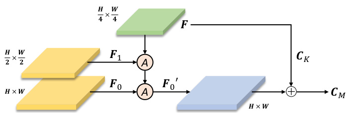
Fig. 5. An overview of the multi-scale contour refinement module. “A” denotes the feature fusion process, following FPN [57].
图 5: 多尺度轮廓细化模块概览。"A"表示特征融合过程,遵循FPN [57]。
Specifically, we first take two additional low-level largescale feature maps from the backbone network (i.e., $F_{0}{\in}$ $\mathbb{R}^{H\times W\times D_{0}}$ and $\begin{array}{r c l}{F_{1}}&{\in}&{\mathbb{R}^{\frac{H}{2}\times\frac{W}{2}\times D_{1}})}\end{array}$ . Note that the highfrequency signals are reserved in ${\cal F}{0}$ and ${\pmb F}{1}$ . Thereafter, as shown in Fig. 5, to aggregate them with the semantically stronger feature map $\pmb{F}$ , we build a simple feature pyramid network [57] to construct feature map $\pmb{F}{0}^{'}\in\mathbb{R}^{H\times W\times\dot{D}_{2}}$ used for following contour refinement.
具体来说,我们首先从主干网络中提取两个额外的低层大尺度特征图(即 $F_{0}{\in}$ $\mathbb{R}^{H\times W\times D_{0}}$ 和 $\begin{array}{r c l}{F_{1}}&{\in}&{\mathbb{R}^{\frac{H}{2}\times\frac{W}{2}\times D_{1}})}\end{array}$)。需要注意的是,高频信号保留在 ${\cal F}{0}$ 和 ${\pmb F}{1}$ 中。随后,如图 5 所示,为了将这些特征图与语义更强的特征图 $\pmb{F}$ 进行聚合,我们构建了一个简单的特征金字塔网络 [57] 来生成用于后续轮廓细化的特征图 $\pmb{F}{0}^{'}\in\mathbb{R}^{H\times W\times\dot{D}_{2}}$。
Based on the feature map $\pmb{F}{0}^{'}$ , we further deform $C_{K}$ to align the object boundary. The contour deformation process is similar to that in the ICD module, except that the GRU-based recurrent update operator is removed. Concretely, given the feature map $\pmb{F}{0}^{'}$ and the current contour $C_{K}$ , we sample the per-vertex features, aggregate them, and directly predict pervertex offset to update the contour $C_{K}$ with a fully connected layer. Finally, we obtain the refined contour estimation, termed as $C_{M}\in\mathbb{R}^{N_{v}\times2}$ , as illustrated in Fig. 2.
基于特征图 $\pmb{F}{0}^{'}$,我们进一步变形 $C_{K}$ 以对齐物体边界。轮廓变形过程与ICD模块类似,只是移除了基于GRU的循环更新算子。具体而言,给定特征图 $\pmb{F}{0}^{'}$ 和当前轮廓 $C_{K}$,我们采样逐顶点特征、聚合这些特征,并通过全连接层直接预测逐顶点偏移量来更新轮廓 $C_{K}$。最终获得精细化轮廓估计结果 $C_{M}\in\mathbb{R}^{N_{v}\times2}$,如图2所示。
$D$ . Training Objectives
$D$ . 训练目标
The training is divided into two stages. Concretely, the ICG and ICD modules are first optimized with the objective as follows,
训练分为两个阶段。具体而言,首先通过以下目标优化ICG和ICD模块,
$$
\mathcal{L}=\mathcal{L}{\mathrm{ICG}}+\mathcal{L}_{\mathrm{ICD}}.
$$
$$
\mathcal{L}=\mathcal{L}{\mathrm{ICG}}+\mathcal{L}_{\mathrm{ICD}}.
$$
Then, we freeze the models and optimize the MCR module with objective $\mathcal{L}_{\mathrm{MCR}}$ . In the following, we separately elaborate them.
随后,我们冻结模型并使用目标函数 $\mathcal{L}_{\mathrm{MCR}}$ 优化MCR模块。下文将分别详述这些步骤。
(1) $\mathcal{L}_{\mathrm{ICG}}$ consists of three terms as follows,
$\mathcal{L}_{\mathrm{ICG}}$ 由以下三项组成,
$$
\mathcal{L}{\mathrm{ICG}}=\mathcal{L}{\mathrm{Y}}+\mathcal{L}{\mathrm{S}}+\mathcal{L}_{\mathrm{B}},
$$
$$
\mathcal{L}{\mathrm{ICG}}=\mathcal{L}{\mathrm{Y}}+\mathcal{L}{\mathrm{S}}+\mathcal{L}_{\mathrm{B}},
$$
where $\mathcal{L}{\mathrm{Y}}$ and $\mathscr{L}{\mathrm{S}}$ are the loss on the predicted center heatmap $\mathbf{Y}$ and offset map $\pmb{S}$ . We follow the classic detector CenterNet [53] to compute $\mathcal{L}{\mathrm{Y}}$ and $\mathscr{L}{\mathrm{S}}$ by only changing the output size of the offset map $\boldsymbol{S}$ from $\frac{H}{R}\stackrel{\cdot}{\times}\frac{W}{R}\stackrel{\cdot}{\times}2N_{v}$ to $\breve{\frac{H}{R}}\times\frac{W}{R}\dot{\times}2$ to directly regress the initial contour with $N_{v}$ vertices. Besides, $\mathscr{L}_{\mathrm{S}}$ is the cross-entropy loss between the predicted boundary map $_B$ and its given ground truth B as follows,
其中 $\mathcal{L}{\mathrm{Y}}$ 和 $\mathscr{L}{\mathrm{S}}$ 分别是预测中心热图 $\mathbf{Y}$ 和偏移图 $\pmb{S}$ 的损失。我们遵循经典检测器 CenterNet [53] 来计算 $\mathcal{L}{\mathrm{Y}}$ 和 $\mathscr{L}{\mathrm{S}}$,仅将偏移图 $\boldsymbol{S}$ 的输出尺寸从 $\frac{H}{R}\stackrel{\cdot}{\times}\frac{W}{R}\stackrel{\cdot}{\times}2N_{v}$ 改为 $\breve{\frac{H}{R}}\times\frac{W}{R}\dot{\times}2$,以直接回归具有 $N_{v}$ 个顶点的初始轮廓。此外,$\mathscr{L}_{\mathrm{S}}$ 是预测边界图 $_B$ 与其给定真实值 B 之间的交叉熵损失,如下所示,
$$
\mathcal{L}{B}=-\sum_{i=1}^{N_{p}}\left[\hat{y}{i}\log(y_{i})+(1-\hat{y}{i})\log(1-y_{i})\right],
$$
$$
\mathcal{L}{B}=-\sum_{i=1}^{N_{p}}\left[\hat{y}{i}\log(y_{i})+(1-\hat{y}{i})\log(1-y_{i})\right],
$$
where $\begin{array}{l}{{N_{p}}=\frac{H}{4}\times\frac{W}{4}}\end{array}$ is the number of pixels in map $B$ $\hat{y}{i}\in[0,1]$ and $\mathbf{\bar{\alpha}}y_{i}\in\bar{{0,1}}$ denote the ground-truth and the predicted confidence score in $\hat{B}$ and $_B$ , respectively.
其中 $\begin{array}{l}{{N_{p}}=\frac{H}{4}\times\frac{W}{4}}\end{array}$ 是特征图 $B$ 中的像素数量,$\hat{y}{i}\in[0,1]$ 和 $\mathbf{\bar{\alpha}}y_{i}\in\bar{{0,1}}$ 分别表示 $\hat{B}$ 和 $_B$ 中的真实置信度得分与预测置信度得分。
(2) $\mathcal{L}_{\mathrm{ICD}}$ is calculated by accumulating the loss over all $K$ iterations as follows,
(2) $\mathcal{L}_{\mathrm{ICD}}$ 的计算方式是对所有 $K$ 次迭代的损失进行累加,具体如下:
$$
\mathcal{L}{\mathrm{ICD}}=\sum_{k=1}^{K}\lambda^{K-k}(\mathcal{L}{R}^{(k)}+\alpha\mathcal{L}_{P}^{(k)}),
$$
$$
\mathcal{L}{\mathrm{ICD}}=\sum_{k=1}^{K}\lambda^{K-k}(\mathcal{L}{R}^{(k)}+\alpha\mathcal{L}_{P}^{(k)}),
$$
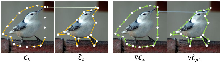
Fig. 6. An illustration of the coordinate regression loss $\mathcal{L}{R}^{(k)}$ (left) and the proposed shape loss $\mathcal{L}{P}^{(k)}$ (right). The loss $\mathcal{L}{R}^{(k)}$ measure the coordinate distance between the predicted contour $C_{k}$ and GT contour $\hat{C}{g t}$ , while $\mathcal{L}_{R}^{(k)}$ encourages the learning of object shape.
图 6: 坐标回归损失 $\mathcal{L}{R}^{(k)}$ (左)与提出的形状损失 $\mathcal{L}{P}^{(k)}$ (右)示意图。损失 $\mathcal{L}{R}^{(k)}$ 衡量预测轮廓 $C_{k}$ 与真实轮廓 $\hat{C}{g t}$ 之间的坐标距离,而 $\mathcal{L}_{R}^{(k)}$ 促进物体形状的学习。
where $\mathcal{L}{R}^{(k)}$ and $\mathcal{L}{P}^{(k)}$ are the coordinate regression loss and our proposed contour shape loss at the iteration, is the temporal weighting factor, and $\alpha$ is the weight of contour shape loss. Here $\lambda$ is less than 1, which means the weight of the loss increases exponentially with the iteration. In Fig. 6, we illustrate the coordinate regression loss $\mathcal{L}{R}^{(k)}$ (left) and the proposed shape loss $\mathcal{L}{P}^{(k)}$ (right). Specifically, we compute the coordinate regression loss by calculating the smooth $L_{1}$ distance [41] between the predicted contour ${C_{k}={p_{k}^{1},p_{k}^{2},...,p_{k}^{N_{v}}}}$ and the ground truth $\hat{C_{g t}}={\hat{p}^{1},\hat{p}^{2},...,\hat{p}^{N_{v}}}$ as follows,
其中 $\mathcal{L}{R}^{(k)}$ 和 $\mathcal{L}{P}^{(k)}$ 分别表示第k次迭代时的坐标回归损失和本文提出的轮廓形状损失,$\lambda$ 是时序权重因子,$\alpha$ 是轮廓形状损失的权重系数。这里 $\lambda$ 小于1,意味着损失权重会随迭代次数呈指数级增长。图6展示了坐标回归损失 $\mathcal{L}{R}^{(k)}$ (左)与提出的形状损失 $\mathcal{L}{P}^{(k)}$ (右)的示意图。具体而言,我们通过计算预测轮廓 $C_{k}={p_{k}^{1},p_{k}^{2},...,p_{k}^{N_{v}}}$ 与真实标注 $\hat{C_{g t}}={\hat{p}^{1},\hat{p}^{2},...,\hat{p}^{N_{v}}}$ 之间的平滑 $L_{1}$ 距离[41]来得到坐标回归损失,计算公式如下:
$$
\mathcal{L}{R}^{(k)}=\sum_{n=1}^{N_{v}}\mathrm{smooth}{L1}(\pmb{p}_{k}^{n},\hat{\pmb{p}}^{n}).
$$
$$
\mathcal{L}{R}^{(k)}=\sum_{n=1}^{N_{v}}\mathrm{smooth}{L1}(\pmb{p}_{k}^{n},\hat{\pmb{p}}^{n}).
$$
$$
\mathcal{L}{P}^{(k)}=\sum_{n=1}^{N_{v}}\mathrm{smooth}{L1}(\Delta\pmb{p}_{k}^{n+1\to n},\Delta\hat{\pmb{p}}^{n+1\to n}).
$$
$$
\mathcal{L}{P}^{(k)}=\sum_{n=1}^{N_{v}}\mathrm{smooth}{L1}(\Delta\pmb{p}_{k}^{n+1\to n},\Delta\hat{\pmb{p}}^{n+1\to n}).
$$
The shape loss encourages the learning of object shape and makes the regressed contour enclose the object tightly.
形状损失 (shape loss) 促使模型学习物体形状,并使回归的轮廓紧密包围目标物体。
(3) $\mathcal{L}{\mathrm{MCR}}$ is calculated as the smooth $L_{1}$ distance [41] between the refined contour ${\cal C}{M}={p_{M}^{1},p_{M}^{2},...,p_{M}^{N_{v}}}$ and its given ground truth $\hat{C_{g t}}$ as follows,
(3) $\mathcal{L}{\mathrm{MCR}}$ 计算为精修轮廓 ${\cal C}{M}={p_{M}^{1},p_{M}^{2},...,p_{M}^{N_{v}}}$ 与其给定真实值 $\hat{C_{g t}}$ 之间的平滑 $L_{1}$ 距离 [41],具体如下:
$$
\mathcal{L}{\mathrm{MCR}}=\sum_{n=1}^{N_{v}}\mathrm{smooth}{L1}(\pmb{p}_{M}^{n},\hat{\pmb{p}}^{n}).
$$
$$
\mathcal{L}{\mathrm{MCR}}=\sum_{n=1}^{N_{v}}\mathrm{smooth}{L1}(\pmb{p}_{M}^{n},\hat{\pmb{p}}^{n}).
$$
IV. EXPERIMENTS
IV. 实验
A. Datasets and Metrics
A. 数据集和指标
Extensive experiments have been conducted on three widely recognized datasets for instance segmentation, as well as two additional datasets specifically focused on scene text detection and lane detection, described in the following.
已在三个广泛认可的实例分割数据集以及两个专门针对场景文本检测和车道检测的数据集上进行了大量实验,具体如下。
SBD [34] dataset consists of 5,623 training and 5,732 testing images, spanning 20 distinct semantic categories. It utilizes images from the PASCAL VOC [58] dataset, but reannotates them with instance-level boundaries. In our study of the SBD dataset, we report the performance of prior works and our PolySnake based on the metrics 2010 VOC $\mathrm{AP}{v o l}$ [59], $\mathrm{AP_{50}}$ , and $\mathrm{AP}{70}$ . $\mathrm{AP}_{v o l}$ is computed as the average of average precision (AP) with nine thresholds from 0.1 to 0.9.
SBD [34] 数据集包含5,623张训练图像和5,732张测试图像,涵盖20个不同的语义类别。该数据集采用PASCAL VOC [58] 数据集的图像,但重新标注了实例级边界。在我们的SBD数据集研究中,基于2010 VOC $\mathrm{AP}{vol}$ [59]、$\mathrm{AP_{50}}$ 和 $\mathrm{AP}{70}$ 指标,报告了先前工作和我们提出的PolySnake的性能表现。$\mathrm{AP}_{vol}$ 是通过0.1至0.9九个阈值的平均精度(AP)取均值计算得出。
TABLE I ABLATIONS OF THE INITIAL CONTOUR GENERATION MODULE ON THE SBD VAL SET [34]. $C_{0}$ AND $C_{K}$ ARE THE OUTPUT CONTOUR OF THE ICG AND ICD MODULES, RESPECTIVELY. SETTINGS USED IN OUR FINAL MODEL ARE UNDERLINED.
表 1: 初始轮廓生成模块在SBD验证集[34]上的消融实验。$C_{0}$和$C_{K}$分别是ICG和ICD模块的输出轮廓。最终模型使用的设置已加下划线。
| 实验 | 轮廓 | 方法 | APvol | AP50 | AP70 |
|---|---|---|---|---|---|
| 边界图 | Co | W/ | 49.5 | 61.2 | 31.9 |
| w/o W/ | 49.3 | 61.0 | 32.2 | ||
| CK | w/o | 59.3 | 66.7 | 54.8 | |
| 顶点数量 | CK | N = 64 | 58.9 | 66.0 | 54.1 |
| N=128 | 59.7 | 66.7 | 54.8 | ||
| N= 192 | 59.2 | 66.2 | 54.3 |
TABLE II ABLATIONS OF THE ITERATIVE CONTOUR DEFORMATION MODULE ON THE SBD VAL SET [34]. SETTINGS USED IN OUR FINAL MODEL ARE UNDERLINED.
表 2: 迭代轮廓变形模块在SBD验证集[34]上的消融实验。最终模型使用的设置已加下划线。
| 实验 | 方法 | APvol | AP50 | AP70 | 参数量 (M) FPS |
|---|---|---|---|---|---|
| ContourFeature | fk gk | 58.6 59.7 | 65.7 66.7 | 53.2 54.8 | 20.3 44.2 22.0 28.8 |
| Update Unit | ConvGRU | 59.7 | 66.7 | 54.8 | 22.0 28.8 |
| ConvLSTM W/ | 59.5 59.7 | 66.4 | 54.6 | 22.1 24.4 | |
| Shared Weights | w/o | 59.6 | 66.7 66.5 | 54.8 55.1 | 22.0 31.0 1 |
| Supervised iters | [1,K] | 59.7 | 66.7 | 54.8 | 22.0 |
| {y} | 58.8 | 66.2 | 54.0 22.0 | ||
| W/ | 59.7 | 66.7 | 54.8 | ||
| Shape Loss | w/o | 59.4 | 66.2 | 54.8 |
Cityscapes [35] dataset is intended for assessing the performance of vision algorithms of semantic urban scene understanding. The dataset contains 5000 images with high-quality annotations of 8 semantic categories. They are further split into 2975, 500, and 1525 images for training, validation, and testing, respectively. Results are evaluated in terms of the AP metric averaged over all categories of the dataset.
Cityscapes [35] 数据集旨在评估语义城市场景理解视觉算法的性能。该数据集包含5000张图像,具有8个语义类别的高质量标注,并进一步划分为2975张训练集、500张验证集和1525张测试集。结果以数据集中所有类别的平均AP (Average Precision) 指标进行评估。
KINS [37] dataset is specifically constructed for amodal instance segmentation [60], which adopts images from the KITTI [61] dataset and annotates them with instance-level semantic annotation. The dataset contains 7474 training and 7517 testing images. We evaluate our approach on seven object categories with the AP metric.
KINS [37] 数据集专为不可见实例分割 (amodal instance segmentation) [60] 而构建,其采用 KITTI [61] 数据集中的图像并进行了实例级语义标注。该数据集包含7474张训练图像和7517张测试图像。我们使用AP (Average Precision) 指标在7个物体类别上评估了所提方法。
COCO [36] dataset stands as a substantial and challenging resource for instance segmentation. It encompasses an extensive collection of images, comprising 115,000 for training, 5,000 for validation, and 20,000 for testing, spanning 80 diverse object categories. A notable feature of the COCO dataset is its inclusion of everyday objects and human figures within its imagery. In our research, we employ the COCO Average Precision (AP) metric as the standard for evaluating the efficacy of other methods and our method.
COCO [36] 数据集是实例分割领域一个庞大且具有挑战性的资源。它包含大量图像,涵盖115,000张训练集、5,000张验证集和20,000张测试集,覆盖80个不同物体类别。该数据集的显著特点是包含了日常物品和人物图像。在我们的研究中,我们采用COCO平均精度(AP)指标作为评估其他方法及我们方法效果的标准。
TABLE III PERFORMANCE OF THE SELECTED ITERATIONS DURING INFERENCE ON THE SBD VAL SET [34]. $C_{0}$ IS OUTPUT INITIAL CONTOUR OF THE ICG MODULE. THE RUNNING EFFICIENCY IS EVALUATED ON A SINGLE RTX $2080\mathrm{TI}$ GPU. THE CONTOUR USED AS THE FINAL OUTPUT OF THE ICD MODULE IS UNDERLINED.
表 III SBD验证集[34]上推理过程中选定迭代的性能表现。$C_{0}$是ICG模块输出的初始轮廓。运行效率在单块RTX $2080\mathrm{TI}$ GPU上评估。作为ICD模块最终输出的轮廓已用下划线标出。
| 轮廓 | APvol | AP50 | AP70 | FPS |
|---|---|---|---|---|
| Co | 49.5 | 61.2 | 31.9 | 51.5 |
| C1 | 56.1 | 65.6 | 49.2 | 48.4 |
| C2 | 58.5 | 66.3 | 53.8 | 45.1 |
| C3 | 59.3 | 66.5 | 54.4 | 37.9 |
| C4 | 59.6 | 66.6 | 54.7 | 34.6 |
| C5 | 59.7 | 66.6 | 54.7 | 30.5 |
| C6 | 59.7 | 66.7 | 54.8 | 28.8 |
| C7 | 59.7 | 66.7 | 54.9 | 26.1 |
| C8 | 59.7 | 66.7 | 54.9 | 23.6 |
| CM | 60.0 | 66.8 | 55.3 | 24.6 |
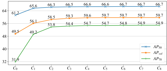
Fig. 7. Performance plot of the selected iterations during inference on the SBD val set [34]. $C_{0}$ is output initial contour of the ICG module.
图 7: 在 SBD 验证集 [34] 上推理过程中选定迭代的性能曲线。$C_{0}$ 是 ICG 模块输出的初始轮廓。
CTW1500 [62] dataset, designed for scene text detection, specifically addresses the challenge of detecting curved texts. It contains 1,500 images, split into 1,000 training and 500 testing images, and features a total of 10,751 text instances, including a significant proportion of curved text. The dataset’s variety includes images sourced from the internet, image libraries, and phone cameras.
CTW1500 [62] 数据集专为场景文本检测设计,特别针对弯曲文本的检测挑战。该数据集包含1,500张图像,分为1,000张训练图像和500张测试图像,共有10,751个文本实例,其中包含大量弯曲文本。数据集的多样性涵盖来自互联网、图像库和手机摄像头的图像。
CULane [63] is a large challenging lane detection dataset. It consists of 9 types of scenarios, including normal, crowd, curve, dazzling light, night, no line, shadow, and arrow. Additionally, it includes a diverse range of environments, capturing both urban and highway settings. In the CULane [63] dataset, the maximum number $M$ of lane lines in the scene is 4.
CULane [63] 是一个大型且具有挑战性的车道检测数据集。它包含9种场景类型,包括正常、拥挤、弯道、眩光、夜间、无线、阴影和箭头。此外,它还涵盖了多样化的环境,包括城市和高速公路场景。在CULane [63]数据集中,场景中车道线的最大数量$M$为4。
B. Implementation Details
B. 实现细节
By default, we set the vertex number $N_{v} = 128$ to form an object contour. The down sampling ratio $R$ and the channel dimension $D$ for feature map $\pmb{F}$ are set as 4 and 64, respectively. The channel dimension $D_{v}$ of contour feature $g_{k,-1}$ is 66. The channel dimension of feature map $F_{0},F_{1}$ , $\pmb{F}{0}^{'}$ in the MCR module are 32, 16, and 8, respectively. We set $\lambda~=~0.8$ and $\alpha=1$ in Equation (9) to calculate loss $\mathcal{L}_{\mathrm{ICD}}$ , respectively. During training, we set the iteration number $K$ as 6 for the SBD [34], Cityscapes [35], COCO [36], and KINS [37] dataset. By default, the iteration number during the inference is the same as that for the training.
默认情况下,我们将顶点数设为 $N_{v} =128$ 以构成物体轮廓。特征图 $\pmb{F}$ 的下采样率 $R$ 和通道维度 $D$ 分别设置为 4 和 64。轮廓特征 $g_{k,-1}$ 的通道维度 $D_{v}$ 为 66。MCR 模块中特征图 $F_{0},F_{1}$ 和 $\pmb{F}{0}^{'}$ 的通道维度分别为 32、16 和 8。在公式 (9) 中,我们设 $\lambda~=~0.8$ 和 $\alpha=1$ 来计算损失 $\mathcal{L}_{\mathrm{ICD}}$。训练时,针对 SBD [34]、Cityscapes [35]、COCO [36] 和 KINS [37] 数据集,我们将迭代次数 $K$ 设为 6。默认情况下,推理阶段的迭代次数与训练阶段相同。

Fig. 8. Example results of the whole contour deformation process on the SBD val set [34]. PolySnake progressively refines the contour. The contour finally converges to a stable position, which tightly encloses the object instance. Zoom in for a better view.
图 8: SBD验证集[34]上完整轮廓变形过程的示例结果。PolySnake逐步优化轮廓,最终收敛到稳定位置,紧密包围目标实例。建议放大查看细节。

Fig. 9. Example results of the contour deformation process on the COCO [36] dataset. PolySnake progressively refines the contour to tightly enclose the object instance. Zoom in for a better view.
图 9: COCO [36] 数据集上轮廓变形过程的示例结果。PolySnake逐步优化轮廓以紧密包围目标实例。放大可查看更佳效果。
C. Ablation Study
C. 消融研究
In this section, we conduct ablations to verify the effectiveness of the main components in our proposed PolySnake, including the initial contour generation, the iterative contour deformation, and the multi-scale contour refinement. Following previous methods [26], [33], all the ablations are studied on the SBD [34] dataset with 20 semantic categories, which well evaluates the algorithm capability to handle various object shapes. Note that in the ablations, our baseline network does not include the multi-scale contour refinement module.
在本节中,我们通过消融实验验证所提PolySnake核心模块的有效性,包括初始轮廓生成、迭代轮廓形变和多尺度轮廓优化。参照先前方法 [26] [33],所有实验均在包含20个语义类别的SBD [34] 数据集上进行,该数据集能有效评估算法处理各类物体形状的能力。需要注意的是,消融实验中的基线网络未包含多尺度轮廓优化模块。
Initial contour generation. We first validate the learning of category-agnostic boundary map $ B$ for the contour initialization. As shown in Table I, with the learning of boundary map $B$ , the performance of contour $C_{0}$ and $C_{K}$ are both slightly improved. This is because the learning of category-agnostic boundary map $_B$ helps to extract a more fine-grained feature map $\pmb{F}$ , which improves the perception of object contour.
初始轮廓生成。我们首先验证了类别无关边界图 $ B$ 的学习对轮廓初始化的作用。如表 1 所示,通过学习边界图 $B$,轮廓 $C_{0}$ 和 $C_{K}$ 的性能均得到小幅提升。这是因为类别无关边界图 $_B$ 的学习有助于提取更精细的特征图 $\pmb{F}$,从而提升对物体轮廓的感知能力。
Furthermore, we test the impact of the vertex number $N_{v}$ to construct a contour. The default vertex number $N_{v}$ of PolySnake is 128. We study the other settings of vertex number $N_{v}$ as 64 and 192, respectively. The results are reported in Table I. It reveals that 128 vertices are enough to represent the contour of an object instance. In contrast, sampling more vertices (192) leads to worse performance. A likely reason is that it is difficult for the contour feature extraction module to obtain a strong representation from an overlong sequence.
此外,我们测试了顶点数量$N_{v}$对轮廓构建的影响。PolySnake默认顶点数$N_{v}$为128,我们分别研究了64和192两种顶点数设置。结果如表1所示,表明128个顶点足以表征物体实例的轮廓。相反,采样更多顶点(192)会导致性能下降,可能原因是轮廓特征提取模块难以从过长的序列中获得强表征。
Iterative contour deformation. We first validate the contour feature extraction used to construct the contour-level representation ${g_{k}}$ of the estimated contour $C_{k}$ . Specifically, as shown in Table II, we train a baseline model that directly feeds the sampled vertex feature $f_{k-1}$ to the recurrent updater (see Fig. 3). In other words, the baseline model does not aggregate the feature of the sampled vertices. With the aggregated vertex feature $g_{k-1}$ , the result shows a performance gain of 1.1 $\mathrm{AP}{v o l}$ . This improvement could be ascribed to the fact that the aggregated feature $g_{k-1}$ encodes stronger context information of the current contour $C_{k-1}$ , which is differentiated and processed by the recurrent updater to estimate further refinement.
迭代轮廓变形。我们首先验证用于构建估计轮廓 $C_{k}$ 的轮廓级表示 ${g_{k}}$ 的轮廓特征提取方法。具体而言,如表 II 所示,我们训练了一个基线模型,该模型直接将采样的顶点特征 $f_{k-1}$ 输入循环更新器 (见图 3)。换句话说,基线模型没有聚合采样顶点的特征。使用聚合顶点特征 $g_{k-1}$ 后,结果显示性能提升了 1.1 $\mathrm{AP}{v o l}$。这一改进可归因于聚合特征 $g_{k-1}$ 编码了当前轮廓 $C_{k-1}$ 更强的上下文信息,这些信息被循环更新器区分和处理以估计进一步的细化。
In the ICD module, the default update unit is the ConvGRU, to which an alternative is the ConvLSTM, a modified version of the standard LSTM [64]. As shown in Table II, while the ConvLSTM shows comparable performance, the ConvGRU produces slightly higher efficiency and accuracy.
在ICD模块中,默认更新单元是ConvGRU,其替代方案是ConvLSTM(标准LSTM [64]的改进版本)。如表II所示,虽然ConvLSTM表现出相当的性能,但ConvGRU在效率和准确度上略胜一筹。
By default, our PolySnake shares the weights across the total $K$ iterations. An alternative version is to learn each vertex feature aggregation module and vertex coordinate update module (see in Sec. III-B) with a distinctive set of weights. In Table II, with the unshared weights, the performances are slightly worse while the parameter number significantly increases. For one thing, this can be attributed to the increased training difficulty of the large model size, which is verified in DeepSnake [26]. For another, our effective information transmission mechanism across iterations and the supervision at each iteration maintain the performance (see Table II), different from DeepSnake [26].
默认情况下,我们的PolySnake在总共$K$次迭代中共享权重。另一种方案是为每个顶点特征聚合模块和顶点坐标更新模块(见第III-B节)学习一组独立的权重。在表II中,使用非共享权重时性能略有下降,而参数量显著增加。一方面,这可以归因于大模型尺寸带来的训练难度提升,这一点在DeepSnake [26] 中得到了验证;另一方面,我们跨迭代的有效信息传输机制和每轮迭代的监督保持了性能(见表II),这与DeepSnake [26] 不同。
We further compare our contour deformation pipeline with the classic DeepSnake [26]. In Fig. 10, we present the results of PolySnake and DeepSnake [26] in terms of the performance (left) and the parameter numbers (right) at different iterations on the SBD val set [34]. In DeepSnake [26], the iteration number is fixed as three by default. On the one hand, simply stacking more refinement modules $(>3)$ introduces extra training and does not necessarily improve the performance; on the other hand, the parameter number increases linearly with more iterations. In contrast, for our PolySnake, the superior performance is obtained after convergence with only a lightweight model, indicating the stronger and stabler contourdeforming ability of our method.
我们进一步将轮廓变形流程与经典方法 DeepSnake [26] 进行对比。图 10 展示了 PolySnake 和 DeepSnake [26] 在 SBD 验证集 [34] 上不同迭代次数下的性能(左)与参数量(右)表现。DeepSnake [26] 默认固定迭代次数为三次:一方面,单纯堆叠更多优化模块 $(>3)$ 会引入额外训练成本且未必提升性能;另一方面,参数量会随迭代次数线性增长。相比之下,我们的 PolySnake 仅需轻量级模型即可在收敛后获得更优性能,这表明本方法具有更强且更稳定的轮廓变形能力。

Fig. 10. Results of DeepSnake [26] and our PolySnake on the performance (left) and the parameter numbers (right) at different time steps on the SBD val set [34]. “ $\cdot_{0},\cdot$ denotes the initial contour for DeepSnake [26] and PolySnake. “ $m^{,}$ represents the MCR module in PolySnake.
图 10: DeepSnake [26] 与我们的 PolySnake 在 SBD val 集 [34] 上不同时间步的性能(左)和参数量(右)对比结果。"$\cdot_{0},\cdot$"表示 DeepSnake [26] 和 PolySnake 的初始轮廓。"$m^{,}$"代表 PolySnake 中的 MCR 模块。
TABLE IV COMPARISON OF THE $\mathrm{AP}{v o l}$ , $\mathrm{AP}{50}$ , AND $\mathrm{AP}_{70}$ PERFORMANCES ON THE SBD VAL SET [34]. “†” MEANS THAT THE MULTI-SCALE CONTOUR REFINEMENT MODULE IS USED.
表 IV: 在 SBD VAL 集 [34] 上 $\mathrm{AP}{vol}$、$\mathrm{AP}{50}$ 和 $\mathrm{AP}_{70}$ 性能对比。"†"表示使用了多尺度轮廓细化模块。
| 方法 | 会议 | APvol | AP50 | AP70 |
|---|---|---|---|---|
| MNC [65] | CVPR'16 | 63.5 | 41.5 | |
| FCIS [66] | CVPR'17 | 65.7 | 52.1 | |
| STS [28] | CVPR'17 | 29.0 | 30.0 | 6.5 |
| ESE-20 [29] | ICCV'19 | 35.3 | 40.7 | 12.1 |
| DeepSnake [26] | CVPR'20 | 54.4 | 62.1 | 48.3 |
| DANCE [32] | WACV'21 | 56.2 | 63.6 | 50.4 |
| EigenContours [52] | CVPR'22 | 56.5 | ||
| E2EC [33] | CVPR'22 | 59.2 | 65.8 | 54.1 |
| PolySnake | 59.7 | 66.7 | 54.8 | |
| PolySnake† | 60.0 | 66.8 | 55.3 |
TABLE V PERFORMANCE COMPARISON WITH OTHER INSTANCE SEGMENTATION METHODS ON THE COCO V A L AND T E S T-D E V SET [36]. “†” MEANS THAT THE MULTI-SCALE CONTOUR REFINEMENT MODULE IS ADDED.
表 5: 在 COCO VAL 和 TEST-DEV 数据集上与其他实例分割方法的性能对比 [36]。"†"表示添加了多尺度轮廓优化模块。
| 方法 | 会议/期刊 | 骨干网络 | AP (val) | AP (test-dev) |
|---|---|---|---|---|
| ESE-Seg [29] | ICCV'19 | Dark-53 | 21.6 | |
| YOLACT [42] | ICCV'19 | R-50-FPN | 28.2 | |
| YOLACT++[67] | TPAMI'20 | R-50-FPN | 34.1 | |
| CenterMask[68] | CVPR'20 | R-50-FPN | 32.9 | |
| PolarMask [24] | CVPR'20 | R-50-FPN | 32.1 | |
| PolarMask++[25] | TPAMI'21 | R-101-FPN | 33.8 | |
| DeepSnake [26] | CVPR'20 | DLA-34 | 30.5 | 30.3 |
| E2EC [33] | CVPR'22 | DLA-34 | 33.6 | 33.8 |
| PolySnake | DLA-34 | 34.4 | 34.5 | |
| PolySnaket | DLA-34 | 34.8 | 34.9 |
During training, we introduce a contour shape loss in Sec. III-D. To validate its effectiveness, we evaluate the performance of our approach with and without it. The results, presented in Table II, reveal that incorporating the contour shape loss yields an improvement of 0.3 in $\mathrm{AP}_{v o l}$ . We attribute this improvement to the fact that the proposed contour shape loss helps the learning of the object shape, which makes the estimated contour enclose the object tightly.
在训练过程中,我们在第 III-D 节引入了轮廓形状损失 (contour shape loss)。为验证其有效性,我们对比了使用与不使用该损失的模型性能。如表 II 所示,引入轮廓形状损失使 $\mathrm{AP}_{v o l}$ 指标提升了 0.3。我们认为这一改进源于该损失函数促进了物体形状的学习,使预测轮廓更紧密地包络目标物体。
Iterative and progressive mechanism. To provide a more specific view of the iterative contour deformation process, we present the performance at the selected iteration in the inference stage. As shown in Table III, the main contour deformation occurs in the top 3 iterations, while the later iterations further progressively fine-tune the result. We also present the performance plots in Fig. 7. As we can see, the results are getting better with iterations and the superior performance is obtained after convergence. These results verify the effectiveness of our method. In our final model, we set the iteration number $K=6$ to strike a balance between the accuracy and the running efficiency. Besides, the contour $C_{M}$ achieves an improvement of $0.5~\mathrm{AP}{70}$ compared with the contour $C_{6}$ , which validates the MCR module that further refines the contour at the full scale.
迭代渐进机制。为了更具体地展示迭代轮廓变形过程,我们在推理阶段选取了特定迭代次数下的性能表现。如表III所示,主要的轮廓变形发生在前3次迭代中,后续迭代则逐步对结果进行微调。图7展示了性能变化曲线,可见随着迭代次数增加,结果持续改善并在收敛后达到最优性能。这些结果验证了我们方法的有效性。在最终模型中,我们将迭代次数设为$K=6$以平衡精度与运行效率。此外,轮廓$C_{M}$相比$C_{6}$实现了$0.5~\mathrm{AP}_{70}$的性能提升,这验证了MCR模块在全尺度上进一步优化轮廓的能力。
As shown in Fig. 8 and Fig. 9, we further visualize the contour deformation process with two samples. It can be seen that, during the contour deformation process, the predicted contours are progressively refined and finally converge to relatively steady positions enclosing the object tightly.
如图 8 和图 9 所示,我们通过两个样本进一步可视化了轮廓形变过程。可以看出,在轮廓形变过程中,预测轮廓会逐步细化,最终收敛到相对稳定的位置并紧密包裹目标物体。
TABLE VI PERFORMANCE COMPARISON ON THE KINS TEST SET [37]. “*” DENOTES WITH ASN PROPOSED IN [69]. “†” MEANS THAT THE MULTI-SCALE CONTOUR REFINEMENT MODULE IS ADDED.
表 6: KINS测试集性能对比 [37]。"*"表示采用[69]提出的ASN。"†"表示添加了多尺度轮廓优化模块。
| 方法 | 会议 | AP |
|---|---|---|
| MNC [65] | CVPR'16 | 18.5 |
| FCIS [66] | CVPR'17 | 23.5 |
| ORCAN [70] | WACV'19 | 29.0 |
| Mask R-CNN [14] | ICCV'17 | 30.0 |
| Mask R-CNN * [69] | CVPR'19 | 31.1 |
| PANet [17] | CVPR'18 | 30.4 |
| PANet *[69] | CVPR'19 | 32.2 |
| VRS&SP[71] | AAAI'21 | 32.1 |
| ARCNN [72] | AI'22 | 32.9 |
| DeepSnake [26] | CVPR'20 | 31.3 |
| E2EC [33] | CVPR'22 | 34.0 |
| PolySnake | 35.0 | |
| PolySnaket | 35.2 |
TABLE VII PERFORMANCE COMPARISON ON THE CTW1500 TEST SET [62]. R, $\mathcal{P}$ , AND $\mathcal{F}$ RESPECTIVELY DENOTE THE RECALL RATE, PRECISION, AND F1-SCORE [73].
表 7: CTW1500测试集上的性能对比 [62]。R、$\mathcal{P}$和$\mathcal{F}$分别表示召回率、精确率和F1分数 [73]。
| 方法 | R | P | F |
|---|---|---|---|
| LOMO [74] | 76.5 | 85.7 | 80.8 |
| PSENet-1s [75] | 79.7 | 84.8 | 82.2 |
| CRAFT [76] | 81.1 | 86.0 | 83.5 |
| DBNet [73] | 80.2 | 86.9 | 83.4 |
| PAN [77] | 81.2 | 86.4 | 83.7 |
| TextDragon [78] | 82.8 | 84.5 | 83.6 |
| DRRG [79] | 83.0 | 85.9 | 84.5 |
| CounterNet [80] | 84.1 | 83.7 | 83.9 |
| PCR [38] | 82.3 | 87.2 | 84.7 |
| TextBPN [81] | 80.6 | 87.7 | 84.0 |
| PAN++ [82] | 81.1 | 87.1 | 84.0 |
| PolySnake | 81.5 | 88.1 | 84.7 |
D. Comparison with State-of-the-art Methods
D. 与现有最优方法的对比
Performance on SBD. PolySnake is implemented in Pytorch [89]. During training, we train the ICG and ICD modules end-to-end for 200 epochs. Then, we freeze their weights and train the MCR module for 50 epochs. The batch size is 40 for both training stages and we use Adam [90] as the optimizer. We use 4 and 2 RTX 2080Ti GPUs for the two training stages, respectively. The learning rate starts from $1e{-}4$ and then decays based on the StepLR strategy. The network is trained and tested at a single scale of $512\times512$ , following [26], [33], following DeepSnake [26].
在SBD上的性能表现。PolySnake采用Pytorch [89]实现。训练过程中,我们端到端训练ICG和ICD模块200个周期,随后冻结其权重并训练MCR模块50个周期。两个训练阶段的批量大小均为40,优化器选用Adam [90]。两个阶段分别使用4块和2块RTX 2080Ti GPU。初始学习率为$1e{-}4$,之后基于StepLR策略进行衰减。遵循DeepSnake [26]和[33]的方法,网络在$512\times512$单尺度下进行训练和测试。
In Table IV, we compare the proposed PolySnake with other contour-based methods [28], [29], [26], [32], [52], [33] on the SBD val set [34]. Our approach achieves $60.0\mathrm{AP}{v o l}$ when the multi-scale contour refinement strategy is adopted. Compared with the classic DeepSnake [26], PolySnake yields $5.6\mathrm{AP}{v o l}$ , 4.7 $\mathrm{AP}{50}$ , and $7.0\mathrm{AP}{70}$ improvements. Besides, PolySnake outperforms the recent state-of-the-art method E2EC [33] by $0.8\mathrm{AP}{v o l}$ , $1.0\mathrm{AP}{50}$ , and $1.2{\ensuremath{\mathrm{AP}}}_{70}$ . We present some qualitative segmentation results of our method in Fig. 11.
在表 IV 中,我们将提出的 PolySnake 与其他基于轮廓的方法 [28]、[29]、[26]、[32]、[52]、[33] 在 SBD val 集 [34] 上进行了比较。当采用多尺度轮廓细化策略时,我们的方法达到了 $60.0\mathrm{AP}{v o l}$。与经典的 DeepSnake [26] 相比,PolySnake 分别实现了 $5.6\mathrm{AP}{v o l}$、4.7 $\mathrm{AP}{50}$ 和 $7.0\mathrm{AP}{70}$ 的提升。此外,PolySnake 以 $0.8\mathrm{AP}{v o l}$、$1.0\mathrm{AP}{50}$ 和 $1.2{\ensuremath{\mathrm{AP}}}_{70}$ 的优势超越了当前最先进的方法 E2EC [33]。我们在图 11 中展示了本方法的一些定性分割结果。
Performance on COCO. For the challenging COCO [36] dataset, we train the ICG and ICD modules following the strategy of E2EC [33]. Then, we freeze them and train the MCR module for another 50 epochs with the same strategy as the SBD [34] dataset. The network is trained at a single image scale of $512\times512$ on 2 RTX 3090Ti GPUs. For the evaluation, we select a model that performs best on the validation set.
在COCO上的性能表现。针对具有挑战性的COCO [36]数据集,我们采用E2EC [33]的策略训练ICG和ICD模块。随后冻结这两个模块,以与SBD [34]数据集相同的策略继续训练MCR模块50个周期。网络在2块RTX 3090Ti GPU上以单图像尺度$512\times512$进行训练。评估时,我们选择在验证集上表现最佳的模型。

Fig. 11. Qualitative results of PolySnake on the SBD val set [34]. Our method can segment object instances correctly in most cases, even when they are in some complex backgrounds or the detected boxes can not cover the objects tightly. It is best viewed in color.
图 11: PolySnake在SBD验证集[34]上的定性结果。我们的方法在多数情况下能正确分割物体实例,即使在复杂背景或检测框未能紧密覆盖物体时。建议彩色查看。

Fig. 12. Qualitative results of PolySnake on the Cityscapes test set [35]. Our method is able to correctly segment objects in most cases, even when they are in complex street scenes. It is best viewed in color.
图 12: PolySnake在Cityscapes测试集[35]上的定性结果。我们的方法在大多数情况下能正确分割物体,即使在复杂的街景中也是如此。建议彩色查看效果最佳。

Fig. 13. Qualitative results of PolySnake on the KINS test set [37]. The top and bottom rows are the input images and their segmentation results, respectively. PolySnake can correctly segment objects with occluded parts in complex scenes. It is best viewed in color.
图 13: PolySnake在KINS测试集[37]上的定性结果。顶行和底行分别为输入图像及其分割结果。PolySnake能在复杂场景中正确分割被遮挡部分的目标物体。建议彩色查看。
As shown in Table V, PolySnake achieves 34.8 and 34.9 AP on the COCO val and test-dev set, respectively. It outperforms the classic DeepSnake [26] by 4.3 and 4.6 AP on the val and test-dev set, respectively. Besides, compared with the recent state-of-the-art method E2EC [33], it achieved a 1.2 and 1.1 AP improvement on the val and test-dev set, respectively.
如表 V 所示,PolySnake 在 COCO val 和 test-dev 数据集上分别取得了 34.8 和 34.9 AP。它在 val 和 test-dev 数据集上分别比经典的 DeepSnake [26] 高出 4.3 和 4.6 AP。此外,与当前最先进的 E2EC [33] 方法相比,它在 val 和 test-dev 数据集上分别实现了 1.2 和 1.1 AP 的提升。
Performance on Cityscapes. As suggested in DeepSnake [26], we apply the component detection strategy [14] to handle the fragmented instances, which are frequently occurred in the dataset. We train the ICG and ICD modules end-to-end for 200 epochs with 16 images per batch on 4 RTX 2080Ti GPUs. Then, their weights are frozen and we train the MCR module for 50 epochs. The Adam optimizer [90] is used, and the learning rate schedule is the same as that for the SBD [34] dataset. We choose the model performing best on the validation set and the evaluation is conducted at a single resolution of $1216\times2432$ , following DeepSnake [26].
在Cityscapes数据集上的表现。如DeepSnake [26]所述,我们采用组件检测策略[14]来处理数据集中频繁出现的碎片化实例。使用4块RTX 2080Ti GPU,以每批次16张图像的配置端到端训练ICG和ICD模块200轮次,随后冻结其权重并训练MCR模块50轮次。优化器采用Adam [90],学习率调度方案与SBD [34]数据集保持一致。遵循DeepSnake [26]的方法,我们选择在验证集上表现最佳的模型,并在单分辨率$1216\times2432$下进行评估。
As shown in Table VIII, we compare our PolySnake with other state-of-the-art methods on the Cityscapes validation and test sets [35]. Using only the fine annotations, our approach achieves superior performances on both the validation and test sets. We outperform DeepSnake [26] by 3.5 AP and 3.4 AP on the validation set and test set, respectively. Compared with recent state-of-the-art E2EC [33], PolySnake achieves a 1.2 AP and 1.7 AP improvement on the validation and test set, respectively. We present some segmentation results in Fig. 12.
如表 VIII 所示,我们在 Cityscapes 验证集和测试集 [35] 上将 PolySnake 与其他先进方法进行了对比。仅使用精细标注时,我们的方法在验证集和测试集上均取得了更优性能。在验证集和测试集上,我们分别以 3.5 AP 和 3.4 AP 的优势超越 DeepSnake [26]。与当前最先进的 E2EC [33] 相比,PolySnake 在验证集和测试集上分别实现了 1.2 AP 和 1.7 AP 的提升。图 12 展示了部分分割结果。
TABLE VIII COMPARISON RESULTS ON THE CITYSCAPES VAL (“AP [V A L]” COLUMN) AND TEST (REMAINING COLUMNS) SETS [35]. USING ONLY FINE TRAINING DATA, POLYSNAKE ACHIEVES SUPERIOR PERFORMANCE ON BOTH THE VAL AND TEST SETS. THE INFERENCE TIME OF METHOD [26], [32], [33] AND POLYSNAKE ARE MEASURED ON A SINGLE RTX 2080TI GPU, WHILE WE REPORT THE RESULTS OF THE OTHER METHODS FROM THEIR ORIGINAL PAPERS. THE BEST AND SECOND-BEST RESULTS IN TOTAL AND EACH CATEGORY ARE HIGHLIGHTED IN BOLD AND UNDERLINED, RESPECTIVELY.
表 VIII CITYSCAPES 验证集 ("AP [VAL]" 列) 和测试集 (其余列) 的对比结果 [35]。仅使用精细标注训练数据时,PolySnake 在验证集和测试集上均取得最优性能。方法 [26]、[32]、[33] 和 PolySnake 的推理时间均在单块 RTX 2080Ti GPU 上测得,其他方法结果来自原论文。总体及各类别最优和次优结果分别用加粗和下划线标出。
| 方法 | 训练数据 | FPS | AP [val] | AP | AP50 | Person | Rider | Car | Truck | Bus | Train | Mcycle | Bicycle |
|---|---|---|---|---|---|---|---|---|---|---|---|---|---|
| SGN [83] | fine +coarse | 0.6 | 29.2 | 25.0 | 44.9 | 21.8 | 20.1 | 39.4 | 24.8 | 33.2 | 30.8 | 17.7 | 12.4 |
| Mask R-CNN [14] | fine | 2.2 | 31.5 | 26.2 | 49.9 | 30.5 | 23.7 | 46.9 | 22.8 | 32.2 | 18.6 | 19.1 | 16.0 |
| GMIS [84] | fine +coarse | - | - | 27.6 | 49.6 | 29.3 | 24.1 | 42.7 | 25.4 | 37.2 | 32.9 | 17.6 | 11.9 |
| Spatial [85] | fine | 11 | - | 27.6 | 50.9 | 34.5 | 26.1 | 52.4 | 21.7 | 31.2 | 16.4 | 20.1 | 18.9 |
| PANet [17] | fine | <1 | 36.5 | 31.8 | 57.1 | 36.8 | 30.4 | 54.8 | 27.0 | 36.3 | 25.5 | 22.6 | 20.8 |
| UPSNet [86] | fine +CocO | 4.4 | 37.8 | 33.0 | 59.6 | 35.9 | 27.4 | 51.8 | 31.7 | 43.0 | 31.3 | 23.7 | 19.0 |
| SSAP [87] | fine | - | 37.3 | 32.7 | 51.8 | 35.4 | 25.5 | 55.9 | 33.2 | 43.9 | 31.9 | 19.5 | 16.2 |
| PolygonRNN++[88] | fine | - | - | 25.5 | 45.5 | 29.4 | 21.8 | 48.3 | 21.1 | 32.3 | 23.7 | 13.6 | 13.6 |
| DeepSnake [26] | fine | 4.6 | 37.4 | 31.7 | 58.4 | 37.2 | 27.0 | 56.0 | 29.5 | 40.5 | 28.2 | 19.0 | 16.4 |
| DANCE [32] | fine | 6.3 | 36.7 | 31.2 | 57.7 | 38.1 | 27.3 | 54.0 | 27.5 | 37.4 | 27.7 | 21.6 | 16.2 |
| E2EC [33] | fine | 4.9 | 39.0 | 32.9 | 59.2 | 39.0 | 27.8 | 56.0 | 28.5 | 41.2 | 29.1 | 21.3 | 19.6 |
| PolySnake | fine | 4.8 | 39.8 | 34.3 | 61.0 | 41.3 | 31.8 | 58.4 | 31.9 | 42.4 | 28.6 | 22.4 | 17.9 |
| PolySnaket | fine | 4.2 | 40.2 | 34.6 | 61.2 | 42.2 | 32.8 | 59.2 | 32.0 | 42.5 | 27.4 | 22.6 | 18.4 |

Fig. 14. Visualization of scene text detection results by the PolySnake on the CTW1500 test set [62]. Best viewed on screen.
图 14: PolySnake在CTW1500测试集[62]上的场景文本检测结果可视化。建议屏幕观看最佳效果。
Performance on KINS. The KINS [37] dataset is used for amodal instance segmentation [60], and is annotated with inference completion information for the occluded parts of the instances. We first train the ICG and ICD modules for 150 epochs with the Adam optimizer [90]. The learning rate starts from $1e-4$ and is decayed by a factor of 0.5 at 80 and 120 epochs. Then, we freeze their weights and train the MCR module for another 50 epochs as the setting for the SBD [34] dataset. Following the classic DeepSnake [26], the models are trained and tested at a single resolution of $512\times512$ and $768\times2496$ , respectively.
KINS数据集上的性能。KINS [37]数据集用于非模态实例分割 [60],并标注了实例遮挡部分的推理补全信息。我们首先使用Adam优化器 [90] 对ICG和ICD模块进行150轮训练,初始学习率为$1e-4$,并在第80和120轮时衰减为原值的0.5倍。随后固定其权重,按照SBD [34] 数据集的配置继续训练MCR模块50轮。遵循经典DeepSnake [26] 方法,模型分别在$512×512$和$768×2496$单分辨率下进行训练和测试。
As shown in Table VI, the MCR module improves the performance from 35.0 AP to 35.2 AP. We note that the improvement is somewhat marginal. A likely reason is that the sampled vertex feature at the occluded parts can not provide the clues for further accurate refinement, different from the other three datasets [34], [35], [36]. Besides, our PolySnake outperforms DeepSnake [26] and E2EC [33] by 3.9 and 1.2 AP, respectively. We present some segmentation results in Fig. 13. It can be seen that the proposed PolySnake can correctly segment objects with occluded parts to each other in complex urban scenes.
如表 VI 所示,MCR模块将性能从35.0 AP提升至35.2 AP。我们注意到这种改进幅度较小,可能原因是与其他三个数据集 [34]、[35]、[36] 不同,遮挡部位采样的顶点特征无法为后续精准优化提供线索。此外,我们的PolySnake分别以3.9 AP和1.2 AP的优势超过DeepSnake [26] 和E2EC [33]。图13展示了部分分割结果,可见所提出的PolySnake能在复杂城市场景中正确分割相互遮挡的物体。
Performance on CTW1500. For scene text detection, the quantitative results on the CTW1500 [62] are presented in Table VII. For this task, we exclusively trained the ICG and ICD modules in an end-to-end manner. The training process spanned 210 epochs, utilizing two 2080Ti GPUs with a batch size of 24. Note that here the vertex number $N_{v}$ of a contour is set as 96, which yields the best optimal performance.
在CTW1500上的表现。针对场景文本检测任务,表VII展示了在CTW1500[62]数据集上的量化结果。该任务中,我们仅以端到端方式训练了ICG和ICD模块。训练过程持续210个周期,使用两块2080Ti GPU,批次大小为24。需注意,此处轮廓顶点数$N_{v}$设为96,该配置可达到最佳性能。
As shown in Table VII, our PolySnake demonstrates outstanding performance. Noteworthy is its remarkable precision, a testament to the accuracy of PolySnake in contour regression. Furthermore, as illustrated in Fig. 14, we further visualize the results of this test benchmark. It is observable that texts of various shapes within the images are accurately segmented. The above exemplary performance in text scenes underscores the robust general iz ability of our PolySnake.
如表 VII 所示,我们的 PolySnake 展现出卓越性能。尤其值得注意的是其惊人的精度,这证明了 PolySnake 在轮廓回归中的准确性。此外,如图 14 所示,我们进一步可视化该测试基准的结果。可以观察到图像中各种形状的文本都被准确分割。上述在文本场景中的优异表现凸显了我们 PolySnake 的强大泛化能力。
TABLE IX COMPARISON RESULTS ON CULANE [63] TEST SET. THE “CROSS” CATEGORY PRESENTS FALSE POSITIVE RESULTS BECAUSE IT HAS NO LANE LINE IN THE SCENARIO. THE BEST AND SECOND-BEST RESULTS IN TOTAL AND EACH CATEGORY ARE HIGHLIGHTED IN BOLD AND UNDERLINED, RESPECTIVE L
表 IX CULANE [63] 测试集上的对比结果。 "交叉"类别由于场景中没有车道线而呈现假阳性结果。总体及各类别的最佳和次佳结果分别用加粗和下划线标出。
| 方法 | 总体 | 正常 | 拥挤 | 炫光 | 阴影 | 无线 | 箭头 | 弯道 | 交叉 | 夜间 |
|---|---|---|---|---|---|---|---|---|---|---|
| SCNN(VGG16)[63] | 71.60 | 90.60 | 69.70 | 58.50 | 66.90 | 43.40 | 84.10 | 64.40 | 1990 | 66.10 |
| CurveLane-NAS-S [91] | 71.40 | 88.30 | 68.60 | 63.20 | 68.00 | 47.90 | 82.50 | 66.00 | 2817 | 66.20 |
| CurveLane-NAS-M[91] | 73.50 | 90.20 | 70.50 | 65.90 | 69.30 | 48.80 | 85.70 | 67.50 | 2359 | 68.20 |
| CurveLane-NAS-L [91] | 74.80 | 90.70 | 72.30 | 67.70 | 70.10 | 49.40 | 85.80 | 68.40 | 1746 | 68.90 |
| PINet (Hourglass) [92] | 74.40 | 90.30 | 72.30 | 66.30 | 68.40 | 49.80 | 83.70 | 65.20 | 1427 | 67.70 |
| RESA(ResNet-34)[93] | 74.50 | 91.90 | 72.40 | 66.50 | 72.00 | 46.30 | 88.10 | 68.60 | 1896 | 69.80 |
| RESA(ResNet-50)[93] | 75.30 | 92.10 | 73.10 | 69.20 | 72.80 | 47.70 | 88.30 | 70.30 | 1503 | 69.90 |
| LaneATT (ResNet-18) [94] | 75.13 | 91.17 | 72.71 | 65.82 | 68.03 | 49.13 | 87.82 | 63.75 | 1020 | 68.58 |
| LaneATT (ResNet-34)[94] | 76.68 | 92.14 | 75.03 | 66.47 | 78.15 | 49.39 | 88.38 | 67.72 | 1330 | 70.72 |
| LaneAF(ERFNet)[95] | 75.63 | 91.10 | 73.32 | 69.71 | 75.81 | 50.62 | 86.86 | 65.02 | 1844 | 70.90 |
| UFLD (ResNet-18) [96] | 68.40 | 87.70 | 66.00 | 58.40 | 62.80 | 40.20 | 81.00 | 57.90 | 1743 | 62.10 |
| UFLD (ResNet-34)[96] | 72.30 | 90.70 | 70.20 | 59.50 | 69.30 | 44.40 | 85.70 | 69.50 | 2037 | 66.70 |
| UFLDv2 (ResNet-18)[97] | 75.00 | 91.80 | 73.30 | 65.30 | 75.10 | 47.60 | 87.90 | 68.50 | 2075 | 70.70 |
| UFLDv2(ResNet-34)[97] | 76.00 | 92.50 | 74.80 | 65.50 | 75.50 | 49.20 | 88.80 | 70.10 | 1910 | 70.80 |
| BézierLaneNet(ResNet-18)[39] | 73.67 | 90.22 | 71.55 | 62.49 | 70.91 | 45.30 | 84.09 | 58.98 | 996 | 68.70 |
| BézierLaneNet(ResNet-34)[39] | 75.57 | 91.59 | 73.20 | 69.20 | 76.74 | 48.05 | 87.16 | 62.45 | 888 | 69.90 |
| PolySnake (ResNet-18) | 75.99 | 91.89 | 74.34 | 70.04 | 73.44 | 48.07 | 87.34 | 68.26 | 1084 | 70.37 |
| PolySnake (ResNet-34) | 76.82 | 92.49 | 75.02 | 68.73 | 75.27 | 48.33 | 87.35 | 67.55 | 899 | 72.30 |

Fig. 15. Visualization of lane detection results by the PolySnake on the CULane dataset [63]. The images in the vertical direction are the original input imag and predictions, respectively. Lane markings are annotated with different colors to indicate different lanes. It is best viewed in color.
图 15: PolySnake在CULane数据集[63]上的车道线检测结果可视化。垂直方向上的图像分别为原始输入图像和预测结果。不同颜色的车道标记表示不同车道。建议彩色查看。
Performance on CULane. For lane detection, the quantitative results on the CULane [63] benchmark dataset are presented in Table IX. We compare our methodology with other prominent approaches, employing ResNet-18 [98] and ResNet34 [98] as backbones. The initial lane line is constructed based on B zi er Lane Net [39]. The vertex number $N_{v}$ of a contour is set as 100, which yields the best optimal performance. It is noteworthy that, in contrast to task instance segmentation and scene text detection, the representation of lane lines is characterized by a sequence of non-closed points. Hence, within the ICD module in Fig. 3, we employ the standard 1-D conventional convolution instead of circle-convolution [26] to perform the vertex feature aggregation.
在CULane上的表现。针对车道线检测任务,表IX展示了CULane [63]基准数据集上的量化结果。我们以ResNet-18 [98]和ResNet-34 [98]为骨干网络,将本方法与其它主流方案进行对比。初始车道线基于B zi er Lane Net [39]构建,轮廓顶点数$N_{v}$设为100时获得最佳性能。值得注意的是,与实例分割和场景文本检测任务不同,车道线表征由非闭合点序列构成。因此,在图3的ICD模块中,我们采用标准一维卷积而非环形卷积[26]进行顶点特征聚合。
PolySnake outperforms many segmentation-based methods on CULane [63]. It also surpasses anchor-based methods, such as LaneATT [94], UFLD [96], and UFLDv2 [97]. The anchorbased methods do not perform well in the dazzle category, where our approach exhibits significantly higher accuracy. Compared with LaneATT [94] that achieves a high total score, our approach surpasses $6.41%$ in the dazzle category on ResNet-18 [98]. Our approach attains the highest F1 score among curve-based approaches, with improvement of $3.15%$ on ResNet-18 [98] and $1.65%$ on ResNet-34 [98] over B zi er Lane Net [39]. Besides, our approach achieves outstanding results in difficult categories, such as night. The visualization results on CULane [63] are presented in Fig. 15.
PolySnake在CULane[63]数据集上优于许多基于分割的方法,同时也超越了基于锚点的方法,如LaneATT[94]、UFLD[96]和UFLDv2[97]。基于锚点的方法在眩光类别表现不佳,而我们的方法在该类别显示出显著更高的准确率。与总分较高的LaneATT[94]相比,我们的方法在ResNet-18[98]上眩光类别提升了6.41%。在基于曲线的方法中,我们的方法取得了最高F1分数,相比BézierLaneNet[39]在ResNet-18[98]和ResNet-34[98]上分别提升了3.15%和1.65%。此外,我们的方法在夜间等困难类别中也取得了优异结果。CULane[63]的可视化结果如图15所示。
V. CONCLUSION
V. 结论
In this work, we introduce PolySnake, a novel deep network architecture for contour-based instance segmentation. PolySnake uniquely combines iterative and progressive learning mechanisms to facilitate the learning of contour estimation. By developing a recurrent architecture, PolySnake maintains a single estimation of a contour for each object instance and progressively updates it toward the object boundary. Through the iterative refinement, the contour finally progressively converges to a stable status that tightly encloses the object instance. Extensive experiments are conducted on several prevalent benchmark datasets across multiple tasks. The results reveal the effectiveness and general iz ability of our PolySnake over existing advanced solutions. For future research, we will explore improving the state-of-the-art instance segmentation methods through effective integration with PolySnake. Moreover, it is significant to excavate our idea on other polygon or curve estimation problems in computer vision.
在本工作中,我们提出了PolySnake——一种基于轮廓的实例分割新型深度网络架构。PolySnake创新性地结合了迭代式与渐进式学习机制来促进轮廓估计的学习。通过开发循环架构,PolySnake为每个物体实例保持单一轮廓估计,并逐步将其更新至物体边界。经过迭代优化,轮廓最终会渐进收敛至紧密包围物体实例的稳定状态。我们在多个任务的流行基准数据集上进行了广泛实验,结果表明PolySnake相比现有先进方案具有显著的有效性和泛化能力。未来研究将探索通过与PolySnake的有效结合来改进最先进的实例分割方法。此外,将我们的思想拓展至计算机视觉中其他多边形或曲线估计问题也具有重要意义。